HAL Id: hal-00350815https://hal.archives-ouvertes.fr/hal-00350815

Preprint submitted on 7 Jan 2009

HAL is a multi-disciplinary open accessarchive for the deposit and dissemination of sci-entific research documents, whether they are pub-lished or not. The documents may come fromteaching and research institutions in France orabroad, or from public or private research centers.

L’archive ouverte pluridisciplinaire HAL, estdestinée au dépôt et à la diffusion de documentsscientifiques de niveau recherche, publiés ou non,émanant des établissements d’enseignement et derecherche français ou étrangers, des laboratoirespublics ou privés.

A discrete contact model for crowd motionBertrand Maury, Juliette Venel

To cite this version:

Bertrand Maury, Juliette Venel. A discrete contact model for crowd motion. 2009. �hal-00350815�

A discrete contact model for crowd motion

Bertrand Maury

Universite de Paris-Sud

UMR du CNRS 8628

F-91405 Orsay Cedex

bertrand.maury@math.u-psud.fr

Juliette Venel

Universite de Paris-Sud

UMR du CNRS 8628

F-91405 Orsay Cedex

juliette.venel@math.u-psud.fr

Abstract

The aim of this paper is to develop a crowd motion model designed to handle highly packed situations. Themodel we propose rests on two principles: We first define a spontaneous velocity which corresponds to thevelocity each individual would like to have in the absence of other people; The actual velocity is then computedas the projection of the spontaneous velocity onto the set of admissible velocities (i.e. velocities which do notviolate the non-overlapping constraint). We describe here the underlying mathematical framework, and weexplain how recent results by J.F. Edmond and L. Thibault on the sweeping process by uniformly prox-regularsets can be adapted to handle this situation in terms of well-posedness. We propose a numerical scheme forthis contact dynamics model, based on a prediction-correction algorithm. Numerical illustrations are finallypresented and discussed.

Resume

Nous proposons un modele de mouvements de foule oriente vers la gestion de configurations tres denses. Cemodele repose sur deux principes: tout d’abord nous definissons une vitesse souhaitee correspondant a lavitesse que les individus aimeraient avoir en l’absence des autres; la vitesse reelle est alors obtenue commeprojection de la vitesse souhaitee sur un ensemble de vitesses admissibles (i.e. qui respectent la contrainte denon-chevauchement). Nous decrivons le cadre mathematique sous-jacent et nous expliquons comment certainsresultats de J.F. Edmond et L. Thibault sur les processus de rafle par des ensembles uniformement prox-reguliers peuvent etre utilises pour prouver le caractere bien pose de notre modele. Nous proposons un schemanumerique pour ce modele de dynamique des contacts base sur un algorithme de type prediction-correction.Enfin des resultats numeriques sont presentes et commentes.

Introduction

Walking behaviour of pedestrians has given rise to a large amount of empirical studies over the last decades.Qualitative data (preferences, walk tendencies) have been collected by Fruin [15], Navin, Wheeler [37], Hender-son [20] and, more recently, by Weidmann [43]. From these observations, several strategies for crowd motionmodelling have been proposed, and can be classified with respect to the way they handle people density (La-grangian description of individuals or macroscopic approach), and to the nature of motion phenomena (deter-ministic or stochastic). Among discrete and stochastic models, let us mention Cellular Automata [2, 7, 36, 38],models based on networks [16] as route choice models [3, 4] and queuing models [31, 44]. In these models, eachcell or node is either empty or occupied by a single person and people’s motion always satisfies this rule. Incellular automata models, there are two manners of moving people during a time step. With the first one, po-sitions are updated one by one with a random order (Random Sequential Update). The second method consistsof updating simultaneously all positions (Parallel Update). If several people want to reach the same cell, onlyone of them (randomly chosen) is allowed to move. In route choice models, people move on a network. Eachmodel is based on a route choice set. Most choice set generation procedures are based on shortest route searchand use shortest paths algorithms. Queuing models use Markov-chain models to describe how pedestrians movefrom one node of the network to another.

In [19], a microscopic model called social force model is presented. It describes crowd motion with a systemof differential equations. The acceleration of an individual is obtained according to Newton’s law. Several forces

1

are introduced as for example a term describing the acceleration towards the desired velocity or a repulsionforce reflecting that a pedestrian tends to keep a certain distance from other people and obstacles. Moreovermacroscopic models have been proposed. In [20], pedestrian traffic dynamics is firstly compared with fluiddynamics. Some models [17, 20, 22] are based on gas-kinetic theory. Other models [23, 24, 25, 26] rest on a setof partial differential equations describing the conservation of flow equation.

Several softwares have been developped: PedGo [21], SimPed [11], Legion [40], Mipsim [22] or Exodus [16].Some commonly observed collective patterns are now considered as standard benchmarks for those numericalsimulations. Among these phenomena of self-organization, there is the formation of lanes formed naturally bypeople moving in opposite directions. In this way, strong interactions with oncoming pedestrians are reduced,and a higher walking speed is possible. Another phenomena is the formation of arches upstream the exitduring the evacuation of a room. These patterns are recovered by CA-models [28, 39] and by the social forcemodel [19, 18].

The case of evacuation in emergency situations is of particular importance in terms of applications (obser-vance of security rules, computer-assisted design of public buildings, appropriate positionning of exit signs).Numerical simulations may allow to estimate evacuation time (to be compared for example with the durationof fire propagation) and also to predict areas where high density will appear. As pointed out by Helbing [18],emergency situations do not fit into the standard framework of pedestrian traffic flow. When people strollaround without hurry, they tend to keep a certain distance from each other and from obstacles. In an emer-gency situation, the motion of individuals is governed by different rules. In particular, the contact with wallsor other people is no longer avoided. Some strategies have been proposed to adapt social walk models to highlycongested situation (see again [18]). We propose here an approach which relies on the very consideration thatactual motion in emergency situations is governed by the opposition between achievement of individual satis-faction (people struggle to escape as quickly as possible, regardless of the global efficiency) and congestion. Inparticular, we aim at integrating the direct conflict between people in the model, in order to estimate in someway interaction forces between them, and therefore provide a way to estimate the local risk of casualties.

The microscopic model we propose rests on two principles. On the one hand, each individual has a spon-taneous velocity that he would like to have in the absence of other people. On the other hand, the actualvelocity must take into account congestion. Those two principles lead us to define the actual velocity field asthe projection of the spontaneous velocity onto the set of admissible velocities (regarding the non-overlappingconstraints). The flexibility of this model lies in its first point: every choice of spontaneous velocity can bemade and so every existing model for predicting crowd motion can be integrated here. The key feature of themodel is the second point which concerns handling of contacts.

By specifying the link between these two velocities, the evolution problem takes the form of a first orderdifferential inclusion. This type of evolution problem has been extensively studied in the 1970’s, with thetheory of maximal monotone operators (see e.g. [6]). A few years later, J.J. Moreau considered similar problemswith time-dependent multivalued operator, namely sweeping processes by convex sets (see [35]). Since then,important improvements have been developped by weakening the convexity assumption with the concept ofprox-regularity. The well-posedness of our evolution problem can be established by means of recent results ofJ.F. Edmond and L. Thibault [13] concerning sweeping processes by uniformly prox-regular sets.

The paper is structured as follows: In Section 2, we present the model and establish its well-posedness; InSection 3, we propose a numerical scheme, and detail the overall solution method. Section 4 is devoted to someillustrations of the numerical algorithm.

1 Modelling

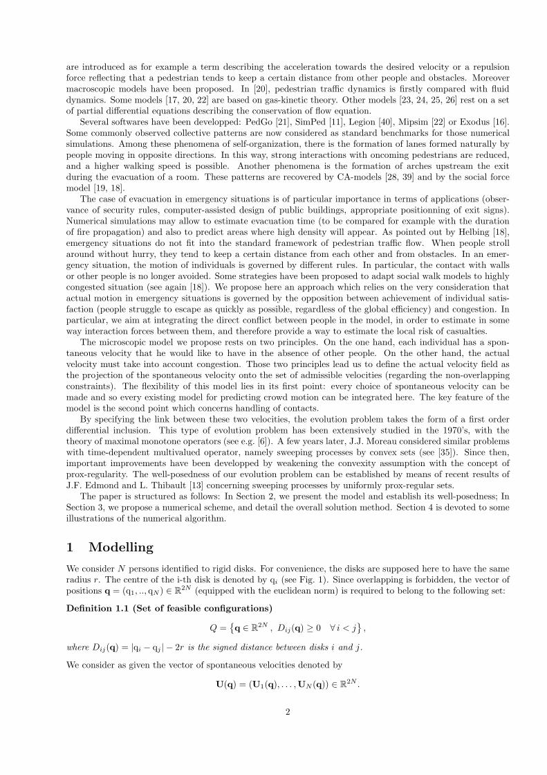
We consider N persons identified to rigid disks. For convenience, the disks are supposed here to have the sameradius r. The centre of the i-th disk is denoted by qi (see Fig. 1). Since overlapping is forbidden, the vector ofpositions q = (q1, .., qN ) ∈ R

2N (equipped with the euclidean norm) is required to belong to the following set:

Definition 1.1 (Set of feasible configurations)

Q ={

q ∈ R2N , Dij(q) ≥ 0 ∀ i < j

}

,

where Dij(q) = |qi − qj | − 2r is the signed distance between disks i and j.

We consider as given the vector of spontaneous velocities denoted by

U(q) = (U1(q), . . . ,UN (q)) ∈ R2N .

2

r

r

eij(q)−eij(q)qj

qi Dij(q)

Figure 1: Notations.

Ui is the spontaneous velocity of individual i, which may depend on its own position (Ui = Ui(qi), see Section 4for examples of such a situation), but also on other people’s positions, that is why we keep here Ui = Ui(q).To define the actual velocity, we introduce the following set:

Definition 1.2 (Set of feasible velocities)

Cq ={

v ∈ R2N , ∀i < j Dij(q) = 0 ⇒ Gij(q) · v ≥ 0

}

,

with

Gij(q) = ∇Dij(q) = (0, . . . , 0,−eij(q), 0, . . . , 0, eij(q), 0, . . . , 0) ∈ R2N and eij(q) =

qj − qi

|qj − qi|.

The actual velocity field is defined as the feasible field which is the closest to U in the least square sense, whichwrites

dq

dt= PCq

U(q),

q(0) = q0 ∈ Q,

(1)

where PCqdenotes the euclidean projection onto the closed convex cone Cq.

Remark 1.3 Despite its formal simplicity, this model does not fit directly into a standard framework. Indeedthe set Cq does not continuously depend on q. If no contact holds, the velocity is not constrained and Cq = R

2N .With a single contact, the set Cq becomes a half-space.

2 Mathematical framework

2.1 Reformulation

Let us reformulate the problem by introducing Nq, the outward normal cone to the set of feasible configurationsQ, which is defined as the polar cone of Cq.

Definition 2.1 (Outward normal cone)

Nq = C◦q

={

w ∈ R2N , w · v ≤ 0 ∀v ∈ Cq

}

.

Remark 2.2 In Figure 2, we represent the set Q ⊂ R2N which is defined as an intersection of convex sets’

complements. In the case of a single contact (configuration q1), we remark that the cone Nq1 is generated bythe vector −G34(q1) that is up to a constant, the outward normal vector to the domain D34 ≥ 0. In the case oftwo or more contacts, the configuration q2 does not belong to a smooth surface and the cone Nq2 (generated by−G12(q2) and −G13(q2)) generalizes somehow the notion of the outward normal direction.

Thanks to Farkas’ Lemma (see [8]), the outward normal cone can be expressed

Nq ={

−∑

λijGij(q) , λij ≥ 0 , Dij(q) > 0 =⇒ λij = 0}

. (2)

Let us recall the classical orthogonal decomposition of a Hilbert space as the sum of mutually polar cone(see [34]) :

PCq+ PNq

= Id. (3)

3

D12 < 0

D13 < 0

D34 < 0

Q0

q2

q1

Nq2

Cq2 Nq1

Cq1

Figure 2: Cones Cq and Nq.

Using this property, we get:dq

dt= PCq

U(q) = U(q) − PNqU(q). (4)

Since PNqU(q) ∈ Nq, we obtain a new formulation for (1)

dq

dt+ Nq ∋ U(q),

q(0) = q0.

(5)

The problem reads as a first order differential inclusion involving the multivalued operator N .

Remark 2.3 In the absence of contacts in the configuration q, the set of feasible velocities Cq is equal to thewhole space R

2N , and consequently the outward normal cone Nq is reduced to {0}. In that case, the first relationof (5) states that the actual velocity equals to the spontaneous velocity:

dq

dt= U(q).

If any contact exists, the differential inclusion means that the configuration q, submitted to U(q), has to evolvewhile remaining in Q.

Let us first study a special situation where standard theory can be applied. Consider N individuals in a corridor.In that case, as people cannot leap accross each other, it is natural to restrict the set of feasible configurationsto one of its connected components:

Q = {q = (q1, . . . , qN ) ∈ RN , qi+1 − qi ≥ 2r}.

In this very situation, as Q is closed and convex, the multivalued operator q 7−→ Nq identifies to the subdiffer-ential of the indicatrix function of Q:

∂IQ(q) = {v, IQ(q) + (v,h) ≤ IQ(q + h) ∀h} , IQ(q) =

∣

∣

∣

∣

0 if q ∈ Q+∞ if q /∈ Q

therefore q 7−→ Nq is maximal monotone. In that case, as soon as the spontaneous velocity is regular (sayLipschitz), standard theory (see e.g. Brezis [6]) ensures well-posedness. Yet, as illustrated in Figure 3, Q isnot convex in general and the operator q 7−→ Nq is not monotone. So we cannot apply the same argumentsas in the case of a straight motion. By lack of convexity, the projection onto Q is not everywhere well-defined.However the set Q satisfies a weaker property in the sense that the projection onto Q is still well-defined in itsneighbourhood. Indeed, Q is uniformly prox-regular, which is the suitable property to ensure well-posedness.Let us give some definitions to specify the general mathematical framework.

4

q2

q1

q2

q1q2q1

configuration q configuration eq configuration q =q + eq

2

Figure 3: Lack of convexity.

ηx

S

Figure 4: η-prox-regular set.

Definition 2.4 Let S be a closed subset of a Hilbert space H.We define the proximal normal cone to S at x by:

N(S,x) = {v ∈ H, ∃α > 0, x ∈ PS(x + αv)} ,

wherePS(y) = {z ∈ S, dS(y) = |y − z|}, with dS(y) = min

z∈S|y − z|.

Following [10], we define the concept of uniform prox-regularity as follows:

Definition 2.5 Let S be a closed subset of a Hilbert space H. S is said η-prox-regular if for all x ∈ ∂S andv ∈ N(S,x), |v| = 1 we have:

B(x + ηv, η) ∩ S = ∅.

In an euclidean space, S is η-prox-regular if an external tangent ball with radius smaller than η can be rolledaround it (see Fig 4). Moreover, this definition ensures that the projection onto such a set is well-defined in itsneighbourhood. The following remark will be useful later.

Remark 2.6 If there exists α > 0 satisfying x ∈ PS(x + αv) then

∀β ≥ 0, β ≤ α, x ∈ PS(x + βv).

Definition 2.7 The proximal subdifferential of function dS at x is the set

∂P dS(x) ={

v ∈ H, ∃M, α > 0, dS(y) − dS(x) + M |y − x|2 ≥ 〈v,y − x〉, ∀y ∈ B(x, α)}

.

Let us specify the useful link between the previous subdifferential and the proximal normal cone, which is provedin [5, 9].

5

Proposition 2.8 The following relation holds true:

∂P dS(x) = NP (S,x) ∩ B(0, 1).

Remark 2.9 A set C ⊂ H is convex if and only if it is ∞-prox-regular. In this case N(C,x) = ∂IC(x) for allx ∈ C.

We now come to the main result of this section.

Theorem 2.10 Assume that U is Lipschitz and bounded. Then, for all T > 0 and all q0 ∈ Q, the followingproblem

dq

dt+ Nq ∋ U(q)

q(0) = q0,

has one and only one absolutely continuous solution q(·) over [0, T ].

This well-posedness can be obtained by using results in [13, 14] as soon as we prove that Q is uniformly prox-regular and that the set Nq identifies to the proximal normal cone to Q at q. This is the core of next subsection.

Remark 2.11 It can be shown that the solution given by Theorem 2.10 satisfies the initial differential equa-tion (4) (see [1]).

2.2 Prox-regularity of Q

Let us consider the setQij = {q ∈ R

2N , Dij(q) ≥ 0}.

Proposition 2.12 Let S be a closed subset of Rn whose boundary ∂S is an oriented C2 hypersurface. For each

x ∈ ∂S, we denote by ν(x) the outward normal to S at x. Then, for each x ∈ ∂S, the proximal normal cone toS at x is generated by ν(x), i.e.

N(S,x) = R+ν(x).

Proof: The proof is a straightforward computation (see [41]). ⊓⊔We can also deduce the expression of the proximal normal cone to Qij .

Corollary 2.13 For all q ∈ Qij,N(Qij ,q) = −R

+Gij(q).

By Definition 2.5, the constant of prox-regularity equals to the largest radius of a “rolling external ball”. Inorder to estimate its radius, tools of differential geometry can be used. More precisely, to show that the set Qij

is uniformly prox-regular, we can apply the following theorem, that is proved in [12].

Theorem 2.14 Let C be a closed convex subset of Rn such that ∂C is an oriented C2 hypersurface of R

n. Wedenote by νC(x) the outward normal to C at x and by ρ1(x), .., ρn−1(x) ≥ 0 the principal curvatures of C at x.We suppose that

ρ = supx∈∂C

sup1≤i≤n−1

ρi(x) < ∞.

Then S = Rn \ int(C) is a η-prox-regular set with η =

1

ρ.

Proposition 2.15 Qij is η0-prox-regular with η0 = r√

2.

6

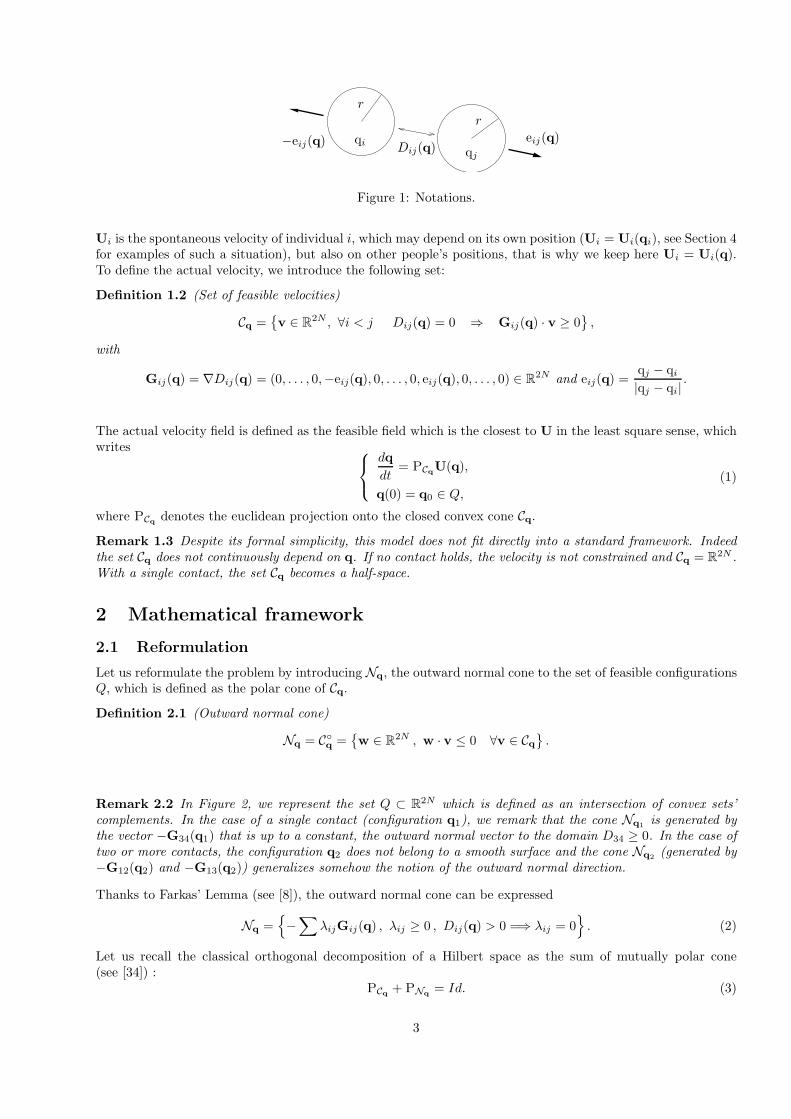
Proof: The set int(Qij) is obviously the complement of a convex set C which satisfies the assumptions ofTheorem 2.14. The constant of prox-regularity of Qij can be obtained by calculating its principal curvatures,which are the eigenvalues of Weingarten endomorphism. Let q ∈ ∂Qij , the outward normal to C at q is equalto −ν(q), where

ν(q) = −Gij(q)√2

=(0, . . . , 0, eij(q), 0, . . . , 0,−eij(q), 0, . . . , 0)√

2.

Weingarten endomorphism is written as follows, for all tangent vectors h ∈ Tq(∂Qij),

Wq(h) := −Dν(q)[h] =1√

2|qj − qi|(

0, . . . , 0,−Pe⊥ij

(hj − hi), 0, . . . , 0,Pe⊥ij

(hj − hi), 0, . . . , 0)

,

withPe⊥

ij(hj − hi) = (hj − hi) − [(hj − hi) · eij ]eij .

After some computations, we deduce that the endomorphism Wq has two eigenvalues, 0 and√

2/|qj − qi|, andthe latter is equal to 1/(r

√2), which ends the proof. ⊓⊔

Now let us study the set of feasible configurations Q, that is the intersection of all sets Qij . We begin todetermine its proximal normal cone.

Proposition 2.16 For all q ∈ Q, N(Q,q) =∑

N(Qij ,q) = Nq.

Proof: The second equality follows from (2) and Proposition 2.15. Let us prove the first one. If q ∈ int(Q),then for each couple (i, j), q ∈ int(Qij), which implies

N(Q,q) = {0} =∑

N(Qij ,q).

We now consider q ∈ ∂Q and introduce the following set:

Icontact = {(i, j), i < j, Dij(q) = 0} = {(i, j), i < j, q ∈ ∂Qij}. (6)

First, we check that N(Qij ,q) ⊂ N(Q,q). Let (i, j) belong to Icontact (otherwise the previous inclusion isobvious), we consider w ∈ N(Qij ,q) \ {0} and we set v = w/|w|. By Proposition 2.8, v ∈ ∂P dQij

(q) and thus

∃M, α > 0, dQij(q) − dQij

(q) + M |q− q|2 ≥ v · (q − q), ∀q ∈ B(q, α).

Since dQij(q) = 0 = dQ(q) and dQij

(q) ≤ dQ(q), it follows that

∃M, α > 0, dQ(q) − dQ(q) + M |q− q|2 ≥ v · (q − q), ∀q ∈ B(q, α).

Therefore v ∈ ∂P dQ(q) and w ∈ N(Q,q). Consequently, for each couple (i, j) ∈ Icontact, we obtain N(Qij ,q) ⊂ N(Q,q)as required. We now want to prove

∑

N(Qij ,q) ⊂ N(Q,q).

It suffices to show that∀w1, w2 ∈ N(Q,q) \ {0} , w = w1 + w2 ∈ N(Q,q).

Let w1 and w2 belong to N(Q,q) \ {0}, we set w = w1 + w2, v1 = w1/|w1| and v2 = w2/|w2|. By Proposi-tion 2.8, there exists M1, M2 ≥ 0, α1, α2 > 0 such that

dQ(q) − dQ(q) + M1|q− q|2 ≥ 〈v1, q − q〉, ∀q ∈ B(q, α1),

dQ(q) − dQ(q) + M2|q− q|2 ≥ 〈v2, q − q〉, ∀q ∈ B(q, α2).

So w = |w1|v1 + |w2|v2 and the vector v = w/|w1| + |w2| satisfies |v| ≤ 1. Furthermore v = tv1 + (1 − t)v2,where

t =|w1|

(|w1| + |w2|).

For α = min(α1, α2) and M = tM1 + (1 − t)M2, the following relation holds

dQ(q) − dQ(q) + M |q− q|2 ≥ v · (q − q), ∀q ∈ B(q, α).

7

Figure 5: Vanishing of the constant of prox-regularity.

Hence v ∈ ∂P dQ(q) and w ∈ N(Q,q). To conclude, it remains to check that

N(Q,q) ⊂∑

N(Qij ,q).

By (3), any w ∈ N(Q,q) can be written w = v + z = PNqw + PCq

w, with v⊥z. Suppose z 6= 0. Sincew ∈ N(Q,q), there exists t > 0 such that q ∈ PQ(q + tw). Let

s = min(t, ǫ) with ǫ = min(i,j)/∈Icontact

Dij(q)√2|z|

,

by Remark 2.6, we know that q ∈ PQ(q + sw). Now set

q = q + sw − sv = q + sz

and show that q ∈ Q. By convexity of Dij , we have

Dij(q) ≥ Dij(q) + s Gij(q) · z, ∀(i, j).

In addition, for (i, j) ∈ Icontact, it yields Gij(q) · z ≥ 0, because z ∈ Cq. Consequently,

∀(i, j) ∈ Icontact, Dij(q) ≥ Dij(q) + s Gij(q) · z = s Gij(q) · z ≥ 0.

Furthermore, if (i, j) /∈ Icontact, then s ≤ Dij(q)√2|z|

. Hence

Dij(q) ≥ Dij(q) + s Gij(q) · z ≥ Dij(q) − s√

2|z| ≥ 0.

That is why q ∈ Q and dQ(q+sw) ≤ |q+sw−q| = s|v|. Yet |q+sw−q| = s|w| > s|v| because |w|2 = |v|2+|z|2.Thus q /∈ PQ(q + sw), which leads to a contradiction. In conclusion, z = 0 and w = v ∈ Nq =

∑

N(Qij ,q),which completes the proof of the proposition. ⊓⊔

Now we want to show the uniform prox-regularity of Q. Since Q does not satisfy the same smoothnessproperties as Qij , the results of differential geometry cannot be applied. By Theorem 2.14, if a set is thecomplement of a smooth convex set, then it is uniformly prox-regular. A natural question arises : Is theintersection of such sets (which is the case for Q) uniformly prox-regular with a constant depending only on theconstants of prox-regularity of the smooth sets. From a general point of view, this is wrong as illustrated inFigure 5. Indeed, we have plotted in solid line the boundary of a set S which is the intersection of two identicaldisks’ complements. This set is uniformly prox-regular but its constant of prox-regularity (equal to the radiusof the disk plotted in dashed line) tends to zero when the disks’ centres move away from each other. In thissituation, the scalar product between normal vectors n1 and n2 (see Figure 6) tends to -1. Thus, the constantof prox-regularity of S is also dependent on the angle between vectors n1 and n2. We now come to the mainresult of this subsection: the uniform prox-regularity of Q. This result rests on an inverse triangle inequalitybetween vectors Gij(q), which is based on angle estimates. Let us point out that we do not claim optimalityof the constant η below.

Proposition 2.17 Q is η-prox-regular with

η ∼ r√

2

23N

1

123N2 .

8

n1n2

Figure 6: Evolution of the angle between vectors n1 and n2.

Proof: We want to prove (cf. Proposition 2.5) that there exists η > 0 such that for all q ∈ Q and for allv ∈ N(Q,q),

v · (q − q) ≤ |v|2η

|q − q|2, ∀q ∈ Q. (7)

By Proposition 2.15, for all q ∈ Qij and all w ∈ N(Qij ,q), we have

w · (q − q) ≤ |w|2η0

|q − q|2, ∀q ∈ Qij . (8)

Inegality (7) is obvious when v = 0. So we consider q ∈ ∂Q and v ∈ N(Q,q) \ {0}. By Proposition 2.16,

v = −∑

(i,j)∈Icontact

αijGij(q), αij ≥ 0.

We recall that Q ⊂ Qij so that by (8) we obtain

(

−∑

αijGij(q))

· (q − q) ≤∑ αij |Gij(q)|

2η0|q − q|2, ∀q ∈ Q.

The sum concerns only couples (i, j) belonging to Icontact but for convenience, this point is omitted in thenotation. As |Gij(q)| =

√2, we get

v · (q − q) ≤ 1√2η0

(

∑

αij

)

|q − q|2, ∀q ∈ Q.

To check Inequality (7), it suffices to find a constant η > 0, independent from αij and from q, satisfying

(

∑

αij

) 1√2η0

≤ 1

2η

∣

∣

∣

∑

αijGij(q)∣

∣

∣,

i.e. such that∣

∣

∣

∑

αijGij(q)∣

∣

∣≥

√2

η

η0

(

∑

αij

)

.

Finally, if we are able to exhibit γ > 0 verifying

∣

∣

∣

∑

αijGij(q)∣

∣

∣≥

√2

γ

(

∑

αij

)

,

then Q will be η-prox-regular with

η =η0

γ=

r√

2

γ.

The problem takes the form of an inverse triangle inequality:

∑

αij |Gij(q)| =√

2∑

αij ≤ γ∣

∣

∣

∑

αijGij(q)∣

∣

∣.

The required result will follow as soon as we prove the main proposition stated below. ⊓⊔

9

Proposition 2.18 (Inverse triangle inequality)There exists γ > 1 such that for all q ∈ Q,

∑

(i,j)∈Icontact

αij |Gij(q)| ≤ γ

∣

∣

∣

∣

∣

∣

∑

(i,j)∈Icontact

αijGij(q)

∣

∣

∣

∣

∣

∣

,

whereIcontact = {(i, j), i < j, Dij(q) = 0} and αij are nonnegative reals.

Constant γ can be fixed as follows

γ =

[

1

2

(

1 −(

1 +

(

1

122N

))−1/2)]−3N

2.

Remark 2.19 Note the sign of coefficients αij . From a general point of view, this inequality is obviously wrongif these coefficients are just assumed real. Indeed, for N large enough, the cardinal of the set Icontact couldbe strictly larger than 2N , which induces a relation between vectors Gij(q) (see Fig. 8 for such a degeneratesituation).

The following elementary lemma asserts an inverse triangle inequality for two vectors.

Lemma 2.20 Let u1 and u2 be two vectors of R2N satisfying u1 · u2 = cos θ|u1||u2|, with cos θ > −1. Then for

all

ν ≥ νθ :=

√

2

1 + cos θ

we have |u1| + |u2| ≤ ν|u1 + u2|.

Proof of the inverse triangle inequality: We propose here a method based on angle estimates with vectors Gij(q)as pointed out in Figure 6. We use a recursive proof on the number of involved vectors. We are going to checkthat there exists δ > 1 such that for all subset I ⊂ Icontact and for all αij > 0,

∑

(i,j)∈I⊂Icontact

αij |Gij(q)| ≤ δ|I|

∣

∣

∣

∣

∣

∣

∑

(i,j)∈I⊂Icontact

αijGij(q)

∣

∣

∣

∣

∣

∣

.

Initialization: Suppose that the cardinality of I equals to 1, in other words, I = {(i, j)}. So we clearly have forall αij > 0 and all δ > 1,

αij |Gij(q)| = |αijGij(q)| ≤ δ|αijGij(q)|. (9)

Recursion assumption:If |J | = p, then we have for all αij > 0

∑

(i,j)∈J⊂Icontact

αij |Gij(q)| ≤ δp

∣

∣

∣

∣

∣

∣

∑

(i,j)∈J⊂Icontact

αijGij(q)

∣

∣

∣

∣

∣

∣

. (10)

Take a subset I ⊂ Icontact with |I| = p + 1. For any

w =∑

(i,j)∈I

αijGij(q),

with αij > 0, we choose (k, l) ∈ I and define J = I \ {(k, l)},

w1 =∑

(i,j)∈J

αijGij(q) and w2 = αklGkl(q).

We need the following lemma which will be later proved.

10

elk ekl

−Fk

−Fl

ql qk

(a) Case 1

ekl elk

−Fl

−Fk

qk ql

(b) Case 2a

ekl elk

−Fl

−Fk

qk ql

(c) Case 2b

Lemma 2.21 If w1 6= 0, the following inequality holds

w1 ·w2

|w1||w2|≥ −κ, with κ =

(

1 +

(

1

12

)2N)−1/2

.

Consequently, if w1 6= 0, from Lemma 2.20, we deduce |w1|+ |w2| ≤√

2

1 − κ|w1+w2| (this inequality obviously

holds for w1 = 0). By denoting δ =

√

2

1 − κ> 1, we get

|w1| + |w2| ≤ δ|w|. (11)

Applying recursion assumption (10) and (11), we obtain

∑

(i,j)∈Icontact

αij |Gij(q)| ≤ αkl|Gkl(q)| + δp|w1| ≤ δp (|w2| + |w1|) ≤ δp+1|w|,

which ends the proof of (9) by recursion. As |Icontact| ≤ 3N , the inverse triangle inequality is checked withγ = δ3N . ⊓⊔

Proof of Lemma 2.21: It suffices to deal with w2 = Gkl(q). By setting

βij =

{

αij if i < j

αji else,

we havew1 = (F1, F2, ..., FN ) where Fp =

∑

βipeip.

Thus, Fk ∈ R2 can be interpreted as a pressure force exerted on the kth person by its neighbours (different from

the individual l). Similarly, −Fk can be seen as a reaction force. We are looking for a lower bound of

∆kl :=w1 · w2

|w1||w2|=

−Fk · ekl − Fl · elk

√2√

∑Ni=1 |Fi|2

.

Case 1: −Fk · ekl ≥ 0 or −Fl · elk ≥ 0

Suppose that, for example (cf figure 7(a)) −Fk · ekl ≥ 0. Using |Fl · elk| ≤ |Fl|, we get

∆kl ≥−Fl · elk√2√∑ |Fi|2

≥ −1√2.

In this case, κ = 2−1/2.Case 2: −Fk · ekl < 0 and −Fl · elk < 0

11

Case 2a: −Fk · ekl ≥ −1

4|Fk| or −Fl · elk ≥ −1

4|Fl|

Suppose that, for example (cf Figure 7(b)), −Fk · ekl ≥ −1

4|Fk|. It can be shown that

−1

4≤ −Fk · ekl√

∑ |Fi|2and

−Fl · elk√

∑ |Fi|2≥ −1,

which yields

∆kl ≥1√2

(

−1

4− 1

)

= − 5

4√

2> −1.

In this case κ = 5/(4√

2).

Case 2b: −Fk · ekl < −1

4|Fk| and −Fl · elk < −1

4|Fl| (cf Figure 7(c)).

We need the following lemma.

Lemma 2.22 There exists k and l different from k and l verifying k 6= l and

|Fk| ≥ ǫ|Fk|,|Fl| ≥ ǫ|Fl|,

with ǫ = 1/122N .

We deduce that∑

|Fi|2 ≥ |Fk|2 + |Fl|2 + |Fk|2 + |Fl|2 ≥ (1 + ǫ2)[

|Fk|2 + |Fl|2]

.

Therefore

|∆kl| ≤1√

1 + ǫ2

(

|Fk| + |Fl|√2√

|Fk|2 + |Fl|2

)

≤ 1√1 + ǫ2

.

In this case, κ =1√

1 + ǫ2, which concludes the proof of Lemma 2.21. ⊓⊔

Proof of Lemma 2.22: We firstly consider

−Fk =

Vk∑

i=1

βkj0,iekj0,i

,

where Vk is the number of neighbours of individual k (individual l excepted) (Vk ≤ 5). As a consequence,

−Fk · ekl =

Vk∑

i=1

βkj0,iekj0,i

· ekl.

There exists k1 ∈ {j0,1, j0,2, ..., j0,Vk} (k1 6= k, l) such that for all i ∈ {1, ..., Vk} βkk1ekk1 · ekl ≤ βkj0,i

ekj0,i· ekl.

It is obvious that

βkk1ekk1 · ekl < −1

6Fk · ekl ≤ − 1

24|Fk|.

In fact, individual k1 is the neighbour who exerts the largest pressure force on person k. As illustrated inFigure 7, individual k is between persons l and k1.

If |Fk1 | ≥1

48|Fk|, then we set k = k1. Else |Fk1 | <

1

48|Fk|, and we produce the same reasoning with

−Fk1 = βk1kek1k +

Vk1∑

i=1

βk1j1,iek1j1,i

,

where Vk1 ≤ 5. Thus,

−Fk1 · ekl = βk1kek1k · ekl +

Vk1∑

i=1

βk1j1,iek1j1,i

· ekl.

12

ekl elk

−Fl

qk ql

qk1

qk2

qki

Figure 7: Construction of sequence (ki)

Since −βk1kek1k · ekl < − 1

24|Fk| and −Fk1 · ekl ≤ |Fk1 | <

1

48|Fk|, we obtain

Vk1∑

i=1

βk1j1,iek1j1,i

· ekl = −Fk1 · ekl − βk1kek1k · ekl < − 1

48|Fk|.

As previously, there exists k2 ∈ {j1,1, j1,2, ..., j1,Vk1} (k2 /∈ {k, k1}), such that

βk1k2ek1k2 · ekl < − 1

4 × 122|Fk|

(Similarly, see Figure 7, individual k1 is between persons k2 and k).

If |Fk2 | ≥1

4

(

1

12

)2

|Fk|, we set k = k2. Else, we continue by defining a sequence (ki) (cf Figure 7) such that

k0 = k

|Fki+1 | <1

4

(

1

12

)i+1

|Fk|

βkiki+1ekiki+1 · ekl < −1

4

(

1

12

)i1

6|Fk|.

It can be shown that ki+1 /∈ {k0, k1, ..ki}. This construction ends at most in N − 2 steps:

∃m < N − 1 satisfying |Fkm| ≥ 1

4

(

1

12

)m

|Fk|.

Finally we setk = km.

Analoguously, we deal with Fl, by constructing a sequence (li) verifying similar properties. We can check thatk 6= l in proving that

{k0, k1, ..km} ∩ {l0, l1, ..lp} = ∅.The proof of Lemma 2.22 is achieved by taking ǫ = 1/12N . ⊓⊔

3 Numerical scheme

3.1 Time-discretization scheme

We present in this section a numerical scheme to approximate the solution to (5). The numerical scheme wepropose is based on a first order expansion of the constraints expressed in terms of velocities. The time interval

13

is denoted by [0, T ]. Let N ∈ N⋆, h = T/N be the time step and tn = nh be the computational times. We

denote by qn the approximation of q(tn). The next configuration is obtained as

qn+1 = qn + h un,

whereun = PCh

qn(U(qn)) with

Chq

= {v ∈ R2N , Dij(q) + h Gij(q) · v ≥ 0 ∀ i < j}.

The scheme can be also interpreted in the following way. Let us introduce the set

Q(q) = {q ∈ R2N , Dij(q) + Gij(q) · (q − q) ≥ 0 ∀ i < j},

which can be seen as an inner convex approximation of Q with respect to q. Note that Q(q) is defined in sucha way that Q is the union of all sets Q(q), q ∈ Q. The scheme can be expressed in terms of position:

qn+1 = PQ(qn)(qn + hU(qn)).

In this form it appears as a prediction-correction algorithm: predicted position vector qn + hU(qn), that maynot be admissible, is projected onto the approximate set of feasible configurations.

Remark 3.1 It is straightforward to check that

qn+1 − qn

h+ N(Q(qn),qn+1) ∋ U(qn), (12)

so that the scheme can also be seen as a semi-implicit discretization of (5), where N(Q(qn),qn+1) approximatesN(Q,qn).

Convergence of this scheme shall be proven in a forthcoming paper.

3.2 Numerical solutions

In the model, the discrete actual velocity un is the projection of the spontaneous velocity onto the approximatedset of feasible velocities. We propose here to solve this projection by a Uzawa algorithm (note that any algorithmcould be used to perform this task). For convenience, explicit dependence of vectors and matrices upon thecurrent configuration is omitted (e.g. U stands for U(qn), Dij for Dij(q

n), etc. . . ). The actual velocity u solvesthe following minimization problem under constraints

u = argminv∈Ch

q

|v − U|2.

Uzawa algorithm is based on a reformulation of this minimization problem in a saddle-point form. We introducethe associated Lagrangian

L (v, µ) =1

2|v − U|2 −

∑

1≤i<j≤N

µij (Dij + h Gij · v) .

and the following linear mapping

B : R2N → R

N(N−1)2

v 7→ −h (Gij · v)i<j

With these notations, the set Chq

can be written:

Chq

=

v ∈ R2N , ∀µ ∈

(

R+)

N(N−1)2 , −

∑

1≤i<j≤N

µij ( Dij + h Gij · v) ≤ 0

=

{

v ∈ R2N , ∀µ ∈

(

R+)

N(N−1)2 , µ · (Bv − D) ≤ 0

}

.

14

Figure 8: A case of non-uniqueness for Kuhn-Tucker multipliers.

where D = D(q) ∈ RN(N−1)/2 is the vector of distances. The existence of a saddle-point

(u, λ) ∈ R2N × (R+)

N(N−1)2

for this problem is well-known (see e.g. [8]) and it is characterized by the next system:

u + tBλ = U

µ · (Bu − D) ≤ 0 , ∀µ ≥ 0

λ · (Bu − D) = 0.

Uzawa algorithm produces two sequences (vk) ∈(

R2N)N

and (µk) ∈(

(R+)N(N−1)

2

)N

according to

µ0 = 0

vk+1 = U − tBµk

µk+1 = Π+

(

µk + ρ[

Bvk+1 − D])

,

where Π+ is the euclidean projection onto the cone of vectors with nonnegative components (a simple cut-off inpractice), and ρ > 0 is a fixed parameter. The algorithm can be shown to converge as soon as 0 < ρ < 2/‖B‖2

(see [8]). More precisely, the sequence (vk) converges to u and it can be shown that the sequence (µk) tends

to some λ ∈ (R+)N(N−1)

2 such that (u, λ) is a saddle-point of L. Notice that in general, the Kuhn-Tuckermultiplier λ is not unique as illustrated in Figure 8. In this case, the configuration of 14 people shows 29contacts, consequently matrix tB is not injective.

Remark 3.2 (Link between local prox-regularity and speed of convergence for Uzawa algorithm) We denote byG the matrix whose columns are vectors Gij , where (i, j) ∈ Icontact (defined by (6)), and we introduce A = tGG.The size of this square matrix is equal to ncontact which is the cardinal of Icontact. By inverse triangle inequality(see Proposition 2.18), there exists a constant γ such that for all λ ∈ (R+)ncontact satisfying |λ|1 = 1, we have

∣

∣

∣

∑

λijGij

∣

∣

∣

2

= tλtGGλ = tλAλ ≥ 2

γ2.

We define, for q ∈ Q, a local parameter γq satisfying

min|λ|1=1

λ≥0

tλAλ =2

γ2q

,

and ηq = r√

2/γq. Let us show that parameter ηq (setting a lower bound of the local prox-regularity of Q atpoint q) and the condition number of matrix A are closely related when A is non-singular. By denoting ηmin

the smallest eigenvalue of A, it follows that

ηmin = min|λ|2=1

tλAλ = min|λ|2≥1

tλAλ ≤ min|λ|2≥1

λ≥0

tλAλ.

Since for all λ, |λ|1 ≤ √ncontact|λ|2, we have

min|λ|2≥1

λ≥0

tλAλ ≤ min|λ|1≥√

ncontact

λ≥0

tλAλ = ncontact min|λ|1≥1

λ≥0

tλAλ.

15

Finally,

ηmin ≤ ncontact min|λ|1≥1

λ≥0

tλAλ = ncontact min|λ|1=1

λ≥0

tλAλ =2ncontact

γ2q

.

Thus

ηmin ≤ 6N

γ2q

.

Furthermore, the condition number of matrix A equals to

cond2(A) = ‖A‖2‖A−1‖2 =ηmax

ηmin.

Since |Gij(q)| =√

2, we obtain ‖A‖2 = ηmax ≥ 2, hence

cond2(A) ≥ 2

ηmin≥

2γ2q

6N≥ 4r2

6η2qN

,

which quantifies how the condition number of A varies with ηq. Since the matrix appearing in Uzawa algorithmis A = tGG, we expect that this algorithm converges less quickly for configurations with low local prox-regularity.In numerical simulations, we noticed indeed that solving the saddle-point problem requires more iterations incase of a jam.

4 Numerical results

In order to illustrate the contact model, we propose here an example of spontaneous velocity. The choice ofthe spontaneous velocity is important because this velocity reflects pedestrian behaviour. A lot of choices areobviously possible. The spontaneous velocity of an individual has to take into account obstacles in the roomand specify how he wants to get around them. So this velocity depends on the room’s geometry but it canbe made dependent on other people positions too. Indeed, it is possible here to integrate individual strategies(deceleration or jam’s avoiding). We refer the reader to [32, 33, 42] for other examples of spontaneous velocity.Here we restrict ourselves to simple behavourial model: people tend to optimize their own path, regardless ofothers.

An example of spontaneous velocity

We consider here the simplest choice for the spontaneous velocity. All the individuals have the same behaviour:they want to reach the exit by following the shortest path avoiding obstacles. Then, the spontaneous velocity’sexpression can be specified:

U(q) = (U0(q1), . . . ,U0(qN )) with U0(x) = −s ∇D(x),

where D(x) represents the geodesic distance between the position x and the nearest exit and s > 0 denotesthe speed. In order to compute D, we have used the Fast Marching Method introduced by R. Kimmel and J.Sethian in [27]. In this method, the value of D is computed at each point of a grid. The value at the exit’snodes is set to zero. Then, the values of the distance at the other points is computed step by step so that adiscrete version of |∇D| = 1 is satisfied. Moreover, the distance at the nodes situated in the obstacles is fixedto a large value, which prevents the shortest path from going across them. In Figure 9, we have considered aroom with 5 obstacles and the exit is situated to the left. We note that by following the built velocity field,people are going to avoid obstacles.

Our aim is to simulate evacuation of any building consisting of several floors. We have chosen an objectoriented programming method and we have implemented this Fast Marching Method in a C++ code. Let usdetail this code. On each floor, the spontaneous velocity is directed by the shortest path avoiding obstacles tothe nearest exit or stairwell. In the stairs, people just want to go down. We have integrated this spontaneousvelocity in the C++ code SCoPI: Simulations of Collections of Interacting Particles developped by A. Lefebvre(see [29, 30]). This code allows us to compute the actual velocity as the projection of the spontaneous velocityas described in Section 3.

16

Figure 9: Contour levels of the geodesic distance D and velocity field U0.

Remark 4.1 Notice that the velocity field produced by this strategy is not continuous as soon as the room isnot convex, which rules out Theorem 2.10. This lack of regularity is not important in practical applications :the places at which it occurs (in particular upstream obstacles) are emptied after a few moments. The mainconsequence is the discontinuity of the future configurations with respect to initial data, which is not surprisingfrom a modelling standpoint.

We propose to illustrate the behaviour of the algorithm in two situations. The first one corresponds to amany-individual evacuation from a square room through a single exit, the second one illustrate the capability ofthe approach to handle complicated geometries. For these two experiments, it will be noticed that the contactsbetween the individuals and the obstacles have to be handled (as the contacts between people). Even if anindividual want to avoid an obstacle, he can be pushed on it by people behind them.

Simple evacuation

We consider the situation of 1000 people which are randomly distributed over a square room. The spontaneousvelocity field corresponds straight pathlines towards the exit at constant speed. As the field has a negativedivergence, it tends to increase the local density, so that congestion is rapidly reached in the neighbourhoodof the exit, and the congestion front propagated upstream as long as it is feeded by incoming people. InFigure 11, we represented the current configuration and the corresponding network of interaction pressures: forany couple of disks in contact, we represent the segment between centers, having its color (from white to black)depend upon the (positive) Kuhn-Tucker multiplier which handles the corresponding contraint. We recover theapparition of arches upstream the exit. The Kuhn-Tucker multipliers λij quantify the way U, the spontaneousvelocity field, does not fit the constraints, and as such they can be interpreted in terms of pressures undergoneby individuals. Although it would be presumptuous at this stage to assimilate λij to an actual measure of thediscomfort experienced by persons i and j, it is obvious that high values for those Kuhn-Tucker multipliers canbe expected on zones where people are likely to be crushed.

Complex geometry

In the second example we consider the evacuation of a floor through exit stairs. A zoom on the geometrynear the exit (together with the isovalues of the geodesic distance function, on which the spontaneous velocityis built) is represented on Figure 10. Figure 12 corresponds to snapshots at times 0s, 5s, 11s, 16s, 41s and75s. Disks are colored according to their initial geodesic distance to the exit. Note that initial ordering is notpreserved during the evacuation. Notice also how a jam forms between snapshots 2 and 3 in the room locatedon the left hand side. This jam decreases significantly the rate at which people exit the room, but it disappears

17

Figure 10: Geometry and isovalues for the geodesic distance.

eventually. The final evacuation time is 109s, to be compared to 48s which corresponds to the evacuation timewithout congestion.

References

[1] F. Bernicot and J. Venel. Existence of sweeping process in banach spaces under directional prox-regularity.submitted, 2008.

[2] V. Blue and J.L. Adler. Cellular automata microsimulation for modeling bi-directional pedestrian walkways.Transportation Research B, 35:293–312, 2001.

[3] A. Borgers and H. Timmermans. City centre entry points, store location patterns and pedestrian routechoice behaviour: A microlevel simulation model. Socio-Economic Planning Sciences, 20:25–31, 1986.

[4] A. Borgers and H. Timmermans. A model of pedestrian route choice and demand for retail facilities withininner-cityshopping areas. Geographycal Analysis, 18:115–128, 1986.

[5] M. Bounkhel and L. Thibault. On various notions of regularity of sets in nonsmooth analysis. NonlinearConvex Anal., 48:223–246, 2002.

[6] H. Brezis. Operateurs Maximaux Monotones et Semi-groupes de contractions dans les espaces de Hilbert.AM, North Holland, 1973.

[7] C. Burstedde, K. Klauck, A. Schadschneider, and J. Zittartz. Simulation of pedestrian dynamics using atwo-dimensional cellular automaton. Physica A, 295:507–525, 2001.

[8] P.G. Ciarlet. Introduction a l’analyse numerique matricielle et a l’optimisation. Masson, Paris, 1990.

[9] F.H. Clarke, Y.S. Ledyaev, R.J. Stern, and P.R. Wolenski. Nonsmooth Analysis and Control Theory.Springer-Verlag, New York, Inc., 1998.

[10] F.H. Clarke, R.J. Stern, and P.R. Wolenski. Proximal smoothness and the lower-c2 property. J. ConvexAnal., 2:117–144, 1995.

18

Figure 11: Arches.

19

Figure 12: Zoom.

20

[11] W. Daamen. Modelling passenger flows in public transport facilities. PhD thesis, Technische UniversiteitDelft, 2004.

[12] J.A. Delgado. Blaschke’s theorem for convex hypersurfaces. J.Differential Geometry, 14:489–496, 1979.

[13] J.F. Edmond and L. Thibault. Relaxation of an optimal control problem involving a perturbed sweepingprocess. Math. Program, Ser. B, 104(2-3):347–373, 2005.

[14] J.F. Edmond and L. Thibault. BVsolutions of nonconvex sweeping process differential inclusion withperturbation. J. Differential Equations, 226(1):135–179, 2006.

[15] J.J. Fruin. Design for pedestrians: A level-of-service concept. Highway Research Record, 355:1–15, 1971.

[16] S. Gwynne, E.R. Galea, P.J. Lawrence, and L. Filippidis. Modelling occupant interaction with fire condi-tions using the buildingexodus evacuation model. Fire safety journal, 36(4):327–357, 2001.

[17] D. Helbing. A fluid-dynamic model for the movement of pedestrians. Complex Systems, 6:391–415, 1992.

[18] D. Helbing, I.J. Farkas, and T. Vicsek. Simulating dynamical features of escape panic. Nature, 407:487,2000.

[19] D. Helbing and P. Molnar. Social force model for pedestrians dynamics. Physical Review E, 51:4282–4286,1995.

[20] L.F. Henderson. The stastitics of crowd fluids. Nature, 229:381–383, 1971.

[21] H.Klupfel and T. Meyer-Konig. Characteristics of the pedgo software for crowd movement and egresssimulation. In E. Galea, editor, Pedestrian and Evacuation Dynamics 2003, pages 331–340, University ofGreenwich, 2003. CMS Press, London.

[22] S.P. Hoogendoorn and P.H.L. Bovy. Gas-kinetic modeling and simulation of pedestrian flows. Transporta-tion Research Record, 1710:28–36, 2000.

[23] S.P. Hoogendoorn and P.H.L. Bovy. Dynamic user-optimal assignment in continuous time and space.Transportation Research B, 38:571–592, 2004.

[24] S.P. Hoogendoorn and P.H.L. Bovy. Pedestrian route-choice and activity scheduling theory and models.Transportation Research B, 38:169–190, 2004.

[25] R. Hughes. The flow of large crowds of pedestrians. Mathematics and Computers in Simulation, 53:367–370,2000.

[26] R. Hughes. A continuum theory for the flow of pedestrians. Transportation Research B, 36(6):507–535,2002.

[27] R. Kimmel and J. Sethian. Fast marching methods for computing distance maps and shortest paths.Technical Report 669, CPAM,Univ. of California, Berkeley, 1996.

[28] A. Kirchner and A. Schadschneider. Simulation of evacuation processes using a bionics-inspired cellularautomaton model for pedestrians dynamics. Physica A, 312:260–276, 2002.

[29] A. Lefebvre. Modelisation numerique d’ecoulements fluide/particules, Prise en compte des forces de lubri-fication. PhD thesis, Universite Paris-Sud XI, Faculte des sciences d’Orsay, 2007.

[30] A. Lefebvre. Numerical simulations of gluey particles. To appear in M2AN, 2008.

[31] G.G. Løvas. Modelling and simulation of pedestrian traffic flow. Transportation Research B, 28:429–443,1994.

[32] B. Maury and J. Venel. Un modele de mouvement de foule. In ESAIM: Proc., volume 18, pages 143–152,2007.

[33] B. Maury and J. Venel. Handling of contacts on crowd motion simulations. In Trafic and Granular Flow’07. Springer, 2009. To appear.

21

[34] J.J. Moreau. Decomposition orthogonale d’un espace hilbertien selon deux cones mutuellement polaires.C. R. Acad. Sci, Ser. I, 255:238–240, 1962.

[35] J.J. Moreau. Evolution problem associated with a moving convex set in a Hilbert space. J. DifferentialEquations, 26(3):347–374, 1977.

[36] K. Nagel. From particle hopping models to traffic flow theory. Transportation Research Record, 1644:1–9,1998.

[37] P.D. Navin and R.J. Wheeler. Pedestrian flow characteristics. Traffic Engineering, 39:31–36, 1969.

[38] A. Schadschneider. Cellular automaton approach to pedestrian dynamics-theory. In M. Schreckenberg andS. D. Sharma, editors, Pedestrian and Evacuation Dynamics, pages 75–85. Springer Berlin, 2001.

[39] A. Schadschneider, A. Kirchner, and K. Nishinari. From ant trails to pedestrian dynamics. Applied Bionicsand Biomechanics, 1:11–19, 2003.

[40] G.K. Still. New computer system can predict human behavior response to building fires. Fire, 84:40–41,1993.

[41] J. Venel. Modelisation mathematique et numerique des mouvements de foule. PhD thesis, UniversiteParis-Sud XI, available at http://tel.archives-ouvertes.fr/tel-00346035/fr, 2008.

[42] J. Venel. Integrating strategies in numerical modelling of crowd motion. In Pedestrian and EvacuationDynamics ’08. Springer, 2009. To appear.

[43] U. Weidmann. Transporttechnik der fussgaenger. Technical Report 90, Schriftenreihe des Instituts furVerkehrsplanung, Transporttechnik, Strassen-und Eisenbahnbau, ETH Zurich, Switzerland, 1993.

[44] S.J. Yuhaski and J.M. Macgregor Smith. Modelling circulation systems in buildings using state dependentqueueing models. Queueing Systems, 4:319–338, 1989.

22