A discontinuous Galerkin approximation for a wall–bounded

Noname manuscript No.(will be inserted by the editor)

A discontinuous Galerkin approximation fora wall–bounded consistent three–componentCahn–Hilliard flow model

Juan Manzanero · Carlos Redondo ·Gonzalo Rubio · Esteban Ferrer · AngelRivero–Jimenez

Received: date / Accepted: date

Abstract We present a high–order discontinuous Galerkin (DG) discretiza-tion for the three–phase Cahn–Hilliard model of [Boyer, F., & Lapuerta, C.(2006). Study of a three component Cahn–Hilliard flow model]. In this model,consistency is ensured with an additional term in the chemical free–energy. Themodel considered in this work includes a wall boundary condition that allowsfor an arbitrary equilibrium contact angle in three–phase flows. The model isdiscretized with a high–order discontinuous Galerkin spectral element methodthat uses the symmetric interior penalty to compute the interface fluxes, andallows for unstructured meshes with curvilinear hexahedral elements. The in-tegration in time uses a first order IMplicit–EXplicit (IMEX) method, suchthat the associated linear systems are decoupled for the two Cahn–Hilliardequations. Additionally, the Jacobian matrix is constant, and identical forboth equations. This allows us to solve the two systems by performing onlyone LU factorization, with the size of the two–phase system, followed by twoGauss substitutions. Finally, we test numerically the accuracy of the schemeproviding convergence analyses for two and three–dimensional cases, includingthe captive bubble test, the study of two bubbles in contact with a wall andthe spinodal decomposition in a cube and in a curved pipe with a “T” junction.

Juan Manzanero (E-mail: [email protected]), Carlos Redondo, Gonzalo Rubio, Es-teban Ferrer,ETSIAE-UPM - School of Aeronautics, Universidad Politecnica de Madrid. Plaza CardenalCisneros 3, E-28040 Madrid, Spain. // Center for Computational Simulation, UniversidadPolitecnica de Madrid, Campus de Montegancedo, Boadilla del Monte, 28660, Madrid, Spain.Angel Rivero-JimenezRepsol Technology Lab Agustın de Betancourt S/N, 28935, Mostoles, Madrid, Spain

2 Juan Manzanero et al.

Keywords Cahn–Hilliard · Computational fluid dynamics · High-Ordermethods · Discontinuous Galerkin.

1 Introduction

The study of multiphase flows is of broad interest for both the scientific com-munity and industrial applications (e.g. oil, gas, and nuclear industries). Mul-tiphase flows study the evolution of two or more immiscible fluids, which tendto segregate and be separated by a thin interface. In this work, we study thedynamics of three dissimilar coexisting phases.

The mathematical modeling of multiphase flows distinguishes two mainapproaches: the sharp and the diffuse interface methods. On the one hand, thesharp interface method considers an infinitely thin interface, which is trackedusing, for example, a level–set method [1, 2]. Then the fluid dynamics equationsfor each individual phase are solved, being two fluids coupled through aninterface condition which enforces mass, momentum, and energy balances [3].On the other hand, in the diffuse interface (or phase field) methods [4, 5] theinterface is regularized and it is provided with a finite, yet thin, thickness. As aresult, the concentration of the phases, and all the thermodynamic properties,vary smoothly across the interface.

Among the different diffuse interface methods, the Cahn–Hilliard typemodels are attracting attention [6, 7, 8, 9, 10, 11, 12, 13, 14, 15]. The Cahn–Hilliard equation integrates the effects of phase separation (segregation) andphase homogenization (mixing) in a free–energy function, which is minimizedas the flow evolves. The Cahn–Hilliard model for two phase flows is the sim-plest, and it has been widely studied in the past [16, 17, 13, 14]. Extendingthe two phase model to three phases is not immediate, since new physical con-siderations should be taken into account: the model has to be consistent, i.e.,if one of the three phases is not present initially, it can not emerge in furthertimes. Besides, it is desirable that the model reduces to the two–phase Cahn–Hilliard model when one of the phases is not present. In this work, we use themodel presented in [18], which solves the consistency problem considering aparticular choice of the chemical free–energy. For N > 4 phases, other methodsthat involve degenerate diffusion coefficients have been developed [10, 19, 20].The model is augmented with the boundary condition developed in [21], whichpermits the prescription of the contact angle between the different phases andthe wall by solving a non–homogeneous Neumann boundary condition.

The three phase model is numerically approximated in space with a high–order Discontinuous Galerkin Spectral Element Method (DGSEM) [22] thatuses the symmetric interior penalty method [23, 24, 25, 26, 27]. The DGSEM

A DG approximation for a wall–bounded consistent 3 component CH flow model 3

is desirable since it allows arbitrary order of accuracy [28, 22], low dissipativeand dispersive errors [29, 30, 31, 32], the representation of arbitrarily three–dimensional complex geometries through the use of unstructured meshes withcurvilinear elements [33], efficient mesh adaptation techniques [34, 35, 36],the design of provably stable schemes [37, 38, 39, 40, 13, 41, 14] and it hasbeen used in the past to discretize multiphase (two phase) flows [42, 43, 14].Other three component Cahn–Hilliard flow models are available and havebeen discretized by means of the finite element method [44], local discon-tinuous Galerkin method [45] or spectral element method [10]. The DGSEMhas been used by the authors to discretize the two component Cahn–Hilliardflow model [13]. To the authors’ knowledge, this is the first implementation ofthe three component Cahn–Hilliard model of [18] in a discontinuous Galerkin(and in particular a discontinuous Galerkin Spectral Element method) frame-work. Even though the DGSEM provides us a framework to construct stableschemes, we have not performed a stability analysis here. This is left for futurework. Nevertheless, our results suggest a stable formulation that provides arobust solver.

Finally, we consider a first order IMplicit–EXplicit (IMEX) time integra-tor. We use an IMEX method since the Cahn–Hilliard equation features alinear fourth order spatial operator (which is solved implicitly), and a non–linear second order spatial operator (which is solved explicitly). Therefore thesolution of the fully–discrete system involves the solution of one linear systemfor each of the Cahn–Hilliard equations. The two linear systems, however, aredecoupled such that the Jacobian matrices are constant in time and identicalfor both Cahn–Hilliard equations. This method permits a resolution approachwhere only one LU factorization is performed for the two equations.

The rest of this work is organized as follows: in Sec. 2 we describe the threecomponent Cahn–Hilliard model. The construction of the discrete DG approx-imation is described in Sec. 3. Lastly, we provide numerical experiments in Sec.4 that assess the accuracy of the method. Final conclusions and discussionscan be found in Sec. 5.

2 Model description

The phase field approach to multiphase flows introduces one scalar field cj perfluid, which represents the relative concentration of phase j (i.e. the volumeoccupied by phase j divided by the total volume) in each space–time point.


The conservation of phases condition, then, reads,

Nphases∑j=1

cj = 1. (1)

In this work, we restrict ourselves to three phase flows, Nphases = 3.

We detail in this section the three–phase model derived in [18]. As usual inphase field methods, each of the concentration fields is subjected to a Cahn–Hilliard diffusion equation. The Cahn–Hilliard equation is such that the evo-lution of the concentration minimizes a free–energy. In [18], the free–energyfunction is,

F [σ]ε (c,∇c) =

∫Ω

(12εF

[σ]0 (c)− 3

8ε (∇c)T σ∇c)dx. (2)

The free–energy contains two terms. The first term contains the chemical free–energy, F [σ]

0 , which in this model is a polynomial function on the three concen-trations c = (c1, c2, c3). The second term is the interfacial energy, where σ isthe interface tension tensor, whose entries are the surface tension coefficientsof all the possible interfaces, σij ,

σ =

0 σ12 σ13σ12 0 σ23σ13 σ23 0

. (3)

The interface tension coefficients σij are positive constants. Finally, ε is theinterface width parameter, which controls the thickness of the diffuse inter-faces.

The Cahn–Hilliard equation is constructed such that the concentrationtime derivatives are proportional to the Laplacian of additional scalar fieldscalled chemical potential, µ = (µ1,µ2,µ3),

cj,t = M0

Σj∇2µj , Σi = σij + σik − σjk, (4)

where the positive constant M0 is called mobility, and Σj are constant coeffi-cients called spreading factors. Although in [18] the authors show an extensionthat allows negative spreading factors, this work only considers positive spread-ing factors. For the three–phase model, the chemical potentials are defined as,

µi = 4ΣTε

3∑j=1j 6=i

(1Σj

[∂Fσ

0∂ci

− ∂Fσ0

∂cj

])− 3

4εΣi∇2ci,

3ΣT

= 1Σ1

+ 1Σ2

+ 1Σ3

. (5)


For simplicity, we define fi as

fi = ΣT3

3∑j=1j 6=i

(1Σj

[∂Fσ

0∂ci

− ∂Fσ0

∂cj

]), i = 1, 2, 3, (6)

to write the chemical potential as µi = 12ε fi −

34εΣi∇

2ci.

The model is completed with the definition of the chemical free–energyF

[σ]0 . In [18] the chemical free–energy is constructed to satisfy two important

properties:

Property 1 Conservative model. If the initial condition satisfies c1(x, 0) +c2(x, 0) + c3(x, 0) = 1, then, for all further times a conservative model main-tains

c1(x, t) + c2(x, t) + c3(x, t) = 1, ∀t > 0. (7)

This property is ensured by an appropriate construction of the chemical poten-tials (5). We sum the three Cahn–Hilliard equations to find that,

(c1 + c2 + c3)t = M0∇2(µ1

Σ1+ µ2

Σ2+ µ3

Σ3

)= 0. (8)

Therefore, it suffices that the chemical potentials satisfy,µ1

Σ1+ µ2

Σ2+ µ3

Σ3= 0, (9)

which they do by construction. The relation (9) allows us to compute the chem-ical potential of one of the phases (typically the third phase) as a function ofthe other two phases,

µ3 = −Σ3

Σ1µ1 −

Σ3

Σ2µ2. (10)

Property 2 Consistent model. If the initial concentrations satisfy cj(x, 0) =0, then

cj(x, t) = 0, ∀t > 0. (11)

As shown in [18], this property is guaranteed with the chemical potential con-struction (5), and an appropriate choice of the chemical free–energy.

We are left with two properties to be satisfied by the chemical free–energyto obtain a consistent model. First, the chemical free–energy of a two–phasesystem (when one of the phases is not present in the flow, e.g. phase three) is,

F[σ]0 (c1, c2, 0) = Fσ12

0 (c1, c2) = σ12c21c

22. (12)

A consistent chemical free–energy must satisfy that if one of the phases is notpresent, the resulting chemical free–energy is equivalent to that of a two–phase


flow for the other two fluids. A natural approach that satisfies this propertyis to add the chemical free–energies for the three possible pairs,

Fσ0,NC = Fσ120 (c1, c2) + Fσ13

0 (c1, c3) + Fσ230 (c2, c3)

= σ12c21c

22 + σ13c

21c

23 + σ23c

22c

23.

(13)

Second, the reduction to a two–phase chemical free–energy is not enoughto guarantee the consistency of the model. If c3(x, 0) = 0, then, to ensurec3,t = 0, the chemical potential µ3 must be algebraically zero. This impliesthat the chemical free–energy must satisfy that(

1Σ1

+ 1Σ2

)∂Fσ

0∂c3

− 1Σ1

∂Fσ0

∂c1− 1Σ2

∂Fσ0

∂c2= 0, if c3 = 0. (14)

Eq. (14) is automatically satisfied if an additional term is added to the incon-sistent chemical free–energy (13),

F[σ]0 = F

[σ]0,NC + c1c2c3 (Σ1c1 +Σ2c2 +Σ3c3)

= σ12c21c

22 + σ13c

21c

23 + σ23c

22c

23 + c1c2c3 (Σ1c1 +Σ2c2 +Σ3c3) .

(15)

The chemical free–energy (15) completes the three–phase model. Note thatthis additional term also cancels when one of the phases is not present, andthe chemical free–energy still reduces to that of a two–phase model (12). As aresult, one Cahn–Hilliard equation (4) per phase is solved, with the chemicalpotential defined in (5) and the chemical free–energy in (15). In practice, since(7) holds, we only solve two Cahn–Hilliard equations (4), and the concentrationof the third phase is obtained from the constraint (1), c3 = 1 − c1 − c2. Itsassociated chemical potential, if needed, is also computed from the other twophases using (10).

2.1 Boundary conditions

The Cahn–Hilliard equation is complemented with an appropriate choice ofthe boundary conditions. Here we adopt a wall boundary condition modelwith non–zero contact angle for the three–phase Cahn–Hilliard equations.

Since the equation is fourth order in space, two boundary conditions mustbe specified, for both the chemical potentials and the concentration [4, 5].To guarantee the phases conservation, we enforce a homogeneous Neumannboundary condition for the chemical potential,

∇µi · n∣∣∣∣∂Ω

= 0. (16)


For two–phase flows, a wall boundary condition with contact angle canbe found in [46]. The latter is achieved with a non–homogeneous Neumannboundary condition for the concentration,

∇c1 · n∣∣∣∣∂Ω

= −4ε

cos θw12c1c2,

∇c2 · n∣∣∣∣∂Ω

= −4ε

cos θw21c1c2 = 4ε

cos θw12c1c2.(17)

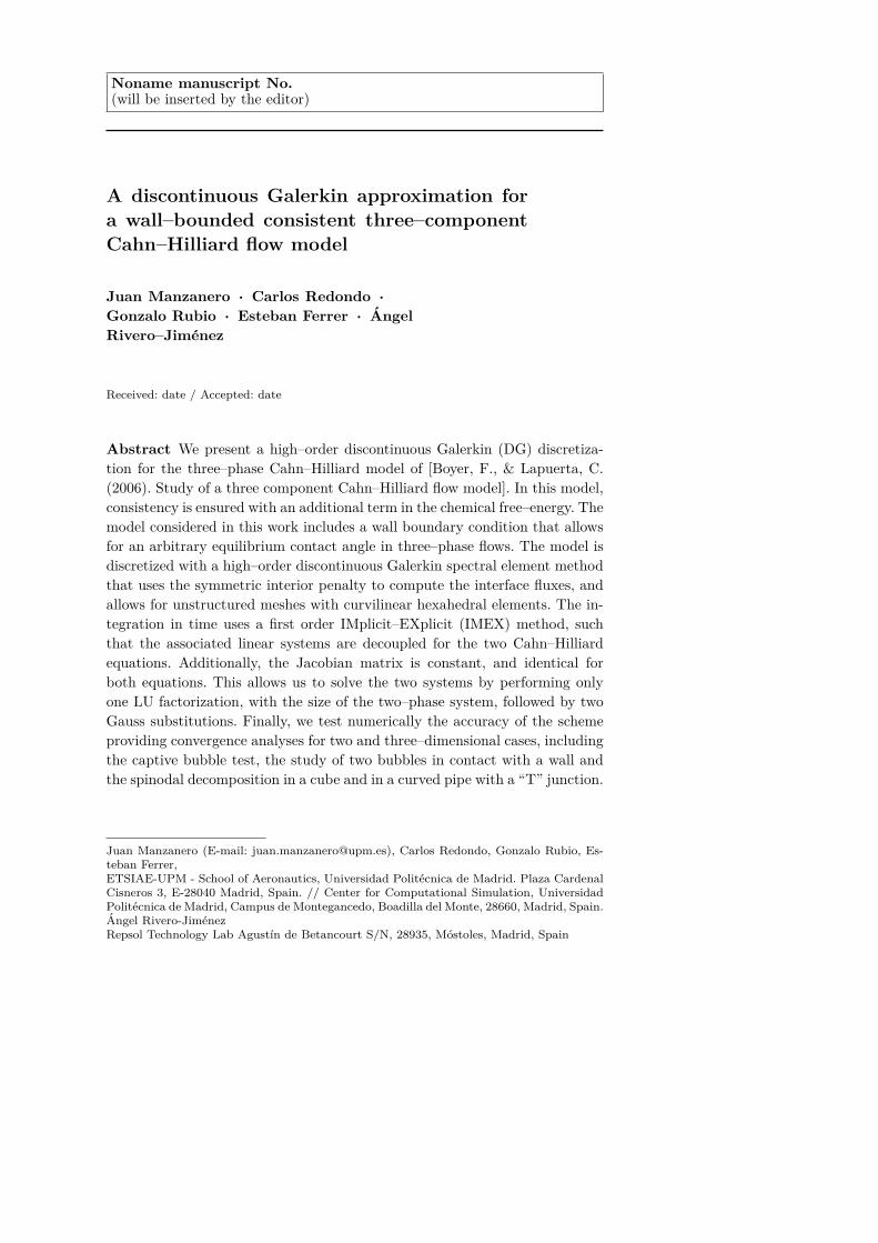
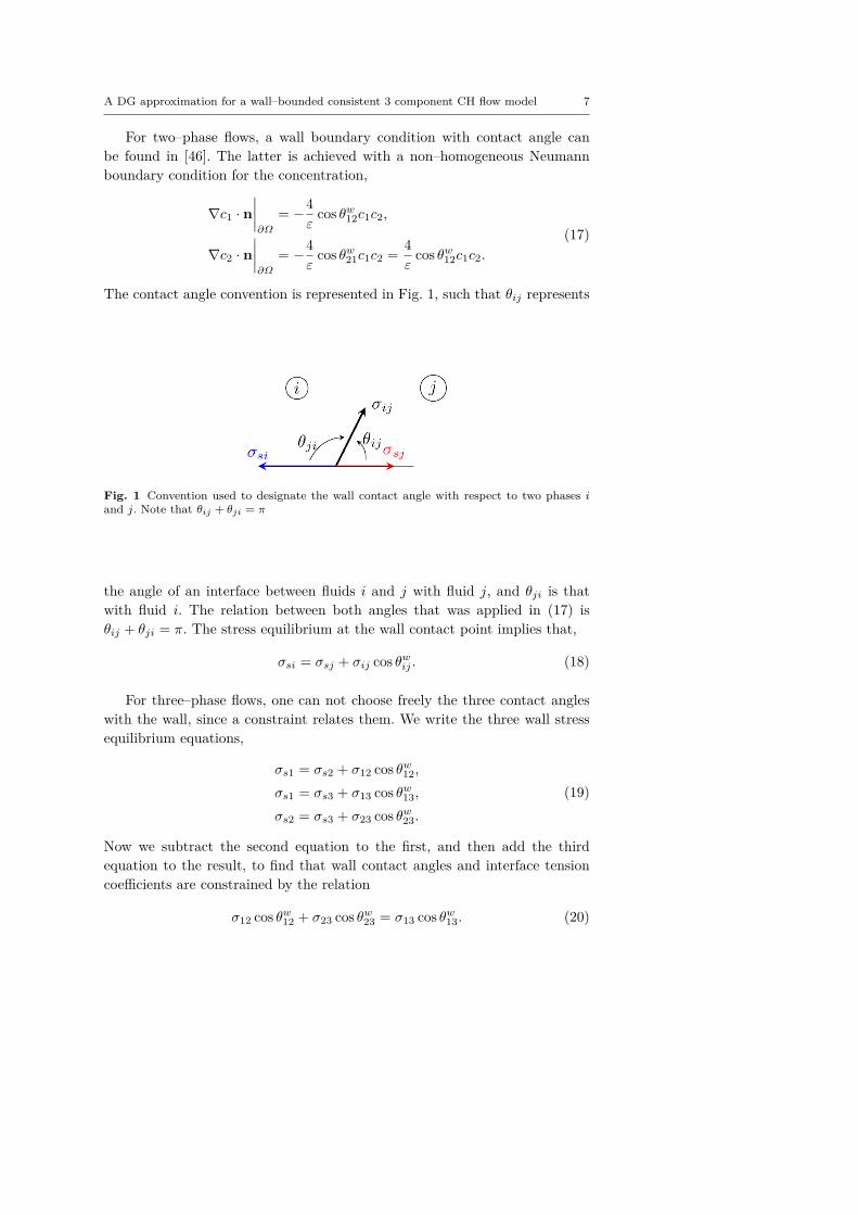
The contact angle convention is represented in Fig. 1, such that θij represents

Fig. 1 Convention used to designate the wall contact angle with respect to two phases iand j. Note that θij + θji = π

the angle of an interface between fluids i and j with fluid j, and θji is thatwith fluid i. The relation between both angles that was applied in (17) isθij + θji = π. The stress equilibrium at the wall contact point implies that,

σsi = σsj + σij cos θwij . (18)

For three–phase flows, one can not choose freely the three contact angleswith the wall, since a constraint relates them. We write the three wall stressequilibrium equations,

σs1 = σs2 + σ12 cos θw12,σs1 = σs3 + σ13 cos θw13,σs2 = σs3 + σ23 cos θw23.

(19)

Now we subtract the second equation to the first, and then add the thirdequation to the result, to find that wall contact angles and interface tensioncoefficients are constrained by the relation

σ12 cos θw12 + σ23 cos θw23 = σ13 cos θw13. (20)


Lastly, in [47, 11] the non–homogeneous Neumann boundary condition wasextended to three phases preserving the consistency property,

∇c1 · n∣∣∣∣∂Ω

= −4ε

[cos θw12c1c2(c1 + c2) + cos θw13c1c3(c1 + c3)] ,

∇c2 · n∣∣∣∣∂Ω

= −4ε

[− cos θw12c1c2(c1 + c2) + cos θw23c2c3(c2 + c3)] ,

∇c3 · n∣∣∣∣∂Ω

= 4ε

[cos θw13c1c3(c1 + c3) + cos θw23c2c3(c2 + c3)] .

(21)

Eq. (21) allows us to conveniently set the wall equilibrium contact angles.

3 Discontinuous Galerkin approximation

In this section we present a novel high–order discontinuous Galerkin approx-imation of the model presented in [18]. Among the different advantages ofthe DG method, exploited in this work, we highlight the capability to con-struct numerical approximations with arbitrarily high order of accuracy andthe use of curvilinear elements in unstructured meshes to represent complexgeometries.

3.1 Approximation and differential geometry

The physical domain Ω is tessellated with non–overlapping hexahedral ele-ments. Then, we use a polynomial transfinite mapping to geometrically trans-form the elements to a reference element E = [−1, 1]3. The mapping relatesphysical (x = (x1,x2,x3) = (x, y, z)) and local (ξ = (ξ1, ξ2, ξ3) = (ξ, η, ζ))coordinates through a function x = X (ξ). The details on how this function isconstructed for a general curvilinear hexahedral can be found in [13].

The transfinite mapping is used to transform curvilinear elements to thereference element E. Associated to the transformation, we can compute thecovariant and contravariant basis, and the Jacobian,

ai = ∂X∂ξi

, ai = ∇ξi = 1J

aj×ak, J = a1 ·(a2 × a3) i = 1, 2, 3, (i, j, k) cyclic.

(22)By construction, the contravariant basis satisfies the continuous metric iden-tities, namely,

3∑i=1

∂Jain∂ξi

= 0, n = 1, 2, 3. (23)


The contravariant basis is also used to transform the differential operatorsinvolved in the equations. The gradient and divergence operators are, (see[33]),

∇u = 1JM~∇ξu, ∇ · f = 1

J∇ξ ·

(MT f

)= 1J∇ξ · f , (24)

where ∇ξ = (∂/∂ξ, ∂/∂η, ∂/∂ζ), andM is the metrics matrix,

M =(Ja1, Ja2, Ja3) . (25)

Additionally, the product of a vector f by the transpose of the metrics matrixM is called a contravariant vector, f .

In the reference element, E, the solution is represented by polynomials ofdegree N , using tensor product Lagrange interpolating polynomials, lj (ξ),

lj(ξ) =N∏i=0i 6=j

ξ − ξiξj − ξi

, j = 0, ...,N . (26)

The Lagrange polynomials are written in a set of Gauss or Gauss–Lobattopoints, ξiNi=0. With the definitions (24), we approximate the solution insidethe reference element as,

u(x, t)∣∣∣∣E

≈ U (ξ, t) =N∑

i,j,k=0Uijk(t)li(ξ)lj(η)lk(ζ). (27)

where the time–dependent nodal degrees of freedom are Uijk(t) = U(ξi, ηj , ζk, t).The convention used in this work is to adopt lower cases for continuous solu-tions, and upper cases for the polynomial approximations. The approximationof the metrics is done differently to (27) to obtain a discrete version of themetric identities (23). Following [33], we compute the contravariant basis as,

J ain = −ei · ∇ξ × IN (Xl∇ξXm) , i,n = 1, 2, 3, (n,m, l) cyclic, (28)

where ei is the unit vector along the i–th spatial direction.

We construct Gauss quadrature rules to approximate integrals inside thereference element. We define the inner product of F and G as their productintegral in the reference element,

〈F ,G〉E =∫E

FGdξ ≈∫E,N

FGdξ = 〈F ,G〉E,N =∑ijk

wijkFijkGijk. (29)


The numerical quadrature weights wijk = wiwjwk are computed from the onedimensional integrals of the Lagrange polynomials,

wi =∫ 1

−1li (ξ)dξ, i = 0, ...,N . (30)

The numerical quadrature exactly approximates the integral of degree 2N ± 1polymomials (+1 for Gauss, -1 for Gauss–Lobatto). Therefore, since the La-grange polymomials satisfy the cardinal property, li (ξj) = δij , they are dis-cretely orthonormal in the reference element,∫ 1

−1,Nli (ξ) lj (ξ)dξ = wiδij , (31)

where δij is the Kronecker delta.

Lastly, given the reference element, the associated surface integral of acontravariant vector f =

(fξ, fη, fζ

)extends to all six faces that define the

element,∫∂E

f · n dSξ =∫Sηζ

fξ dη dζ

∣∣∣∣ξ=1

ξ=−1+∫Sξζ

fη dξ dζ

∣∣∣∣η=1

η=−1+∫Sξη

fζ dξ dη

∣∣∣∣ζ=1

ζ=−1, (32)

where n is the outward pointing normal vector to the six faces of the refer-ence element, dSξ is the surface differential in reference space. The discreteapproximation of surface integrals is computed using the quadrature rules intwo dimensions,∫∂E,N

f · n dSξ =∫Sηζ ,N

fξ dη dζ

∣∣∣∣ξ=1

ξ=−1+∫Sξζ ,N

fη dξ dζ

∣∣∣∣η=1

η=−1+∫Sξη ,N

fζ dξ dη

∣∣∣∣ζ=1

ζ=−1,

=N∑

j,k=0wjkf

ξ (ξ, ηj , ζk)∣∣∣∣ξ=1

ξ=−1+

N∑i,k=0

wikfη (ξi, η, ζk)

∣∣∣∣η=1

η=−1

+N∑

i,j=0wijf

ζ (ξi, ηj , ζ)∣∣∣∣ζ=1

ζ=−1.

(33)

We can represent surface integrals in both physical and reference space. Therelation between physical and reference integration variables is,

dSi = |aj × ak|dξj dξk = |Jai|dξj dξk = J if dSiξ (34)


where i = 1, 2, 3 and J if = |Jai| is the face Jacobian. Moreover, from thedefinition of contravariant fluxes we get,

f · ni dSiξ =(MT f

)· ni dSiξ = f · Jai dSiξ = f · n dS. (35)

Therefore, we can write,∫∂E,N

f · n dSξ =∫∂e,N

f · n dS, (36)

being e an element in physical coordinates, and E the reference element.

3.2 Discontinuous Galerkin approximation of the three–phase model

The Cahn–Hilliard equation is fourth order in space. Thus, to construct a DGapproximation, we rewrite the two Cahn–Hilliard equations as a four equationsystem of first order equations per phase. To do so, we introduce the auxiliaryvariables gc,i = ∇ci and gµ,i = ∇µi so that,

ci,t = M0

Σi∇ · gµ,i,

gµ,i = ∇µi,

µi = 12εfi(c1, c2, c3)− 3

4Σiε∇ · gc,i,

gc,i = ∇ci.

(37)

Recall that fi was defined in (6). Next, we transform the gradient and diver-gence operators to the reference space using (24),

Jci,t = M0

Σi∇ξ · gµ,i,

Jgµ,i =M∇ξµi,

Jµi = 12εJfi(c1, c2, c3)− 3

4Σiε∇ξ · gc,i,

Jgc,i =M∇ξci.

(38)


We construct one weak form for each of the four equations. To do so, wemultiply by arbitrary order N polynomials, ϕi, and integrate in E,

〈Jci,t,ϕc〉E = M0

Σi〈∇ξ · gµ,i,ϕc〉E ,⟨

Jgµ,i,ϕgµ⟩E

=⟨M∇ξµi,ϕgµ

⟩E

=⟨∇ξµi, ϕgµ

⟩E

,

〈Jµi,ϕµ〉E = 12ε〈Jfi,ϕµ〉E −

34Σiε 〈∇ξ · gc,i,ϕµ〉E ,⟨

Jgc,i,ϕgc⟩E

=⟨M∇ξci,ϕgc

⟩E

=⟨∇ξci, ϕgc

⟩E

.

(39)

Note that in the second and fourth equations we have moved the metrics matrixto the vector test function to obtain contravariant test functions. Finally, weapply integration-by-parts to all integrals containing differential operators, andwrite the resulting surface integrals in physical space using (36),

〈Jci,t,ϕc〉E = M0

Σi

(∫∂e

ϕcgµ,i · n dS − 〈gµ,i,∇ξϕc〉E

),⟨

Jgµ,i,ϕgµ⟩E

=∫∂e

µiϕgµ · n dS −⟨µi,∇ξ · ϕgµ

⟩E

,

〈Jµi,ϕµ〉E = 12ε〈Jfi,ϕµ〉E −

34Σiε

(∫∂e

ϕµgc,i · n dS − 〈gc,i,∇ξϕµ〉E

),

⟨Jgc,i,ϕgc

⟩E

=∫∂e

ciϕgc · n dS −⟨ci,∇ξ · ϕgc

⟩E

.

(40)

We introduce the polynomial approximation ansatz in (40). We replacecontinuous functions by the order N polynomials and the exact integrals bythe quadrature rules (29) and (33),

〈JCi,t,ϕc〉E,N = M0

Σi

(∫∂e,N

ϕcG?µ,i · n dS −

⟨Gµ,i,∇ξϕc

⟩E,N

),⟨

JGµ,i,ϕgµ⟩E,N

=∫∂e,N

µ?iϕgµ · n dS −⟨µi,∇ξ · ϕGµ

⟩E,N

,

〈J µi,ϕµ〉E,N = 12ε〈JFi,ϕµ〉E,N −

34Σiε

(∫∂e,N

ϕµG?c,i · n dS −

⟨Gc,i,∇ξϕµ

⟩E,N

),

⟨JGc,i,ϕgc

⟩E

=∫∂e,N

C?i ϕgc · n dS −⟨Ci,∇ξ · ϕgc

⟩E,N .

(41)

Since no continuity requirements to the discrete solution have been imposedat the inter–element faces, the boundary integrals are not uniquely defined.Thus, we replace the solution at the inter–element boundaries by an unique


solution, represented with the star. The inter–element solution and fluxes areresponsible for the coupling between adjacent elements and the enforcementof boundary condition at the physical boundaries. In this work, we use thesymmetric interior penalty method (IP),

C?i = Ci, G?c,i = ∇Ci−σ JCiK , µ?i = µi, G?

µ,i = ∇µi−σ JµiK ,(42)

where the gradients are locally computed using (24), σ is the penalty parametercomputed with the estimation by [48],

σ = (N + 1)(N + 2)2 max

|Jf |J−1

, (43)

and the jump operator accounts the face normal vectors,

JuK = uLnL + uRnR. (44)

The evolution equation for the coefficients is obtained replacing the testfunction by the Lagrange polynomials ϕ = li (ξ) lj(η)lk(ζ).

3.3 Boundary conditions

The boundary conditions enforcement is performed through the numericalfluxes at the physical boundaries. For the chemical potential gradient, we usea homogeneous Neumann boundary condition. Thus, the chemical potential istaken from the interior element, and the normal gradient is set to zero,

µ?i = µi, G?µ,i · n = 0, in ∂e ∩ ∂Ω. (45)

For the concentration, we apply the non–homogeneous Neumann boundarycondition that accounts for arbitrary wall contact angle (21). Thus, we use theinterior value for the concentration, and the normal gradients are set to,

C?i = Ci,

G?c,1 · ~n = −4

ε(cos θw12C1C2 (C1 + C2) + cos θw13C1 (1− C1 − C2) (1− C2)) ,

G?c,2 · ~n = −4

ε(− cos θw12C1C2 (C1 + C2) + cos θw23C2 (1− C1 − C2) (1− C1)) .

(46)

As in the continuous boundary condition, the wall contact angles θwij are sub-jected to the constitutive constraint (20).


3.4 Time discretization

The semi–discrete scheme (41) is complemented with the numerical integra-tion of the left hand side time derivative coefficients. Looking at the continuousequation (4), with chemical potential (5), one finds a linear bi–Laplacian oper-ator for the concentration ci, and a non–linear Laplacian term correspondingto the chemical free–energy derivatives. The bi–Laplacian operator involvesfourth order derivatives, which translates in a severe numerical stiffness thatrestricts the time–step size in explicit solvers. Since the bi–Laplacian operatoris linear, but the Laplacian of the chemical potential is non–linear, a commonlyadopted technique is to use an IMplicit–EXplicit (IMEX) method [20, 13, 14].

We revisit the continuous setting (4)

ci,t = M0∇2(

12Σiε

fi −34ε∇

2ci

)(47)

to describe the approximation in time. We use the IMEX version of the firstorder Euler method described in [20]. We define the coefficients cn = c(tn) asthe solution evaluated in tn, such that we evaluate the chemical free–energyin the old time step, tn, and the interfacial energy in the new time step, tn+1,

cn+1i − cni∆t

= M0∇2(

12Σiε

fi(cn1 , cn2 , cn3 ) + S0(cn+1i − cni

)− 3

4∇2cn+1i

). (48)

The term S0(cn+1i − cni

)stabilizes the non–linear terms, where S0 is a positive

constant, while retaining first order accuracy. Note that the addition of thestabilization term modifies the Jacobian of the implicit solver, but maintainsthe linearity in cn+1

i . Note that this implementation has two advantages:

1. The implicit system is decoupled: for each of the two phases, an individuallinear system only involving cn+1

i is solved.2. The Jacobian matrix of the implicit solver is identical for the two phases.

Hence, only one Jacobian matrix needs to be computed and stored. Thismatrix is constant in time due to the linearity.

In this work, the linear system of equations is solved with an LU factorizationand Gauss substitution. Since the Jacobian matrix is constant in time, and theLU factorization is done only one time at the beginning of the computations.However, the algorithm does not restrict to other techniques, e.g. iterativesolvers.

Finally, we introduce the IMEX scheme (48) in the semi–discrete DG for-mulation (41). To do so, in the definition of the chemical potential (the thirdequation of (41)), we evaluate the chemical free–energy tn, the interfacial en-


ergy in tn+1, and we add the dissipative term S0(Cn+1i − Cni

). As a result,

the chemical potential is evaluated in a mixed IMEX state, which we call µθ,used to evaluate the rest of the variable. We get the fully–discrete system,⟨J C

n+1i − Cni∆t

,ϕc⟩E,N

= M0

Σi

(∫∂e,N

ϕcG?,θµ,i · n dS −

⟨Gθµ,i,∇ξϕc

⟩E,N

),⟨

JGθµ,i,ϕgµ

⟩E,N

=∫∂e,N

µ?,θi ϕgµ · n dS −

⟨µθi ,∇ξ · ϕGµ

⟩E,N

,

⟨J µθi ,ϕµ

⟩E,N = 12

ε

⟨JFni + S0

(Cn+1i − Cni

),ϕµ

⟩E,N ,

− 34Σiε

(∫∂e,N

ϕµG?,n+1c,i · n dS −

⟨Gn+1c,i ,∇ξϕµ

⟩E,N

),

⟨JGn+1

c,i ,ϕgc⟩E

=∫∂e

C?,n+1i ϕgc · n dS −

⟨Cn+1i ,∇ξ · ϕgc

⟩E,N .

(49)

The interested reader can find more details in [20, 13].

4 Numerical experiments

In this section we perform numerical experiments to evaluate the scheme pre-sented and its numerical implementation. We first study the accuracy of thescheme with a convergence analysis, which solves a manufactured solution.Then, we study the captive bubble test, where a bubble is immersed betweenthe two other phases. Lastly, we test the wall contact angle boundary conditionsolving two bubbles of two different phases immersed in the third phase.

4.1 Convergence analysis

We perform a two–dimensional convergence analysis based on the manufac-tured solution used in [20] to solve four phase flows,

c1,m(x, y; t) = 13 (1 + cos (4πx) sin (4πy) sin (t)) ,

c2,m(x, y; t) = 13 (1 + cos (4πx) sin (4πy) sin (1.2t)) ,

(50)

with the physical parameters given in Table 1. The physical domain is Ω =[−1, 1]2, and we enforce periodic boundary conditions at the four physicalboundaries. We solve the fully–discrete system (49) in a uniform Cartesian 22


Table 1 List of the parameter values used with the manufactured solution (50)

σ12 σ13 σ23 M0 ε S0 ∆t6.236E-3 7.265E-3 8.165E-3 1.0E-3 0.1 0.0 1.0E-4

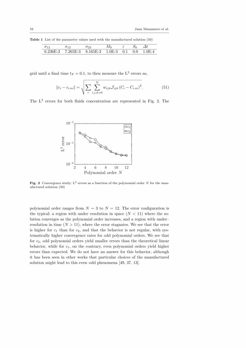
grid until a final time tF = 0.1, to then measure the L2 errors as,

‖ci − ci,m‖ =

√√√√∑e

N∑i,j,k=0

wijkJijk (Ci − Ci,m)2. (51)

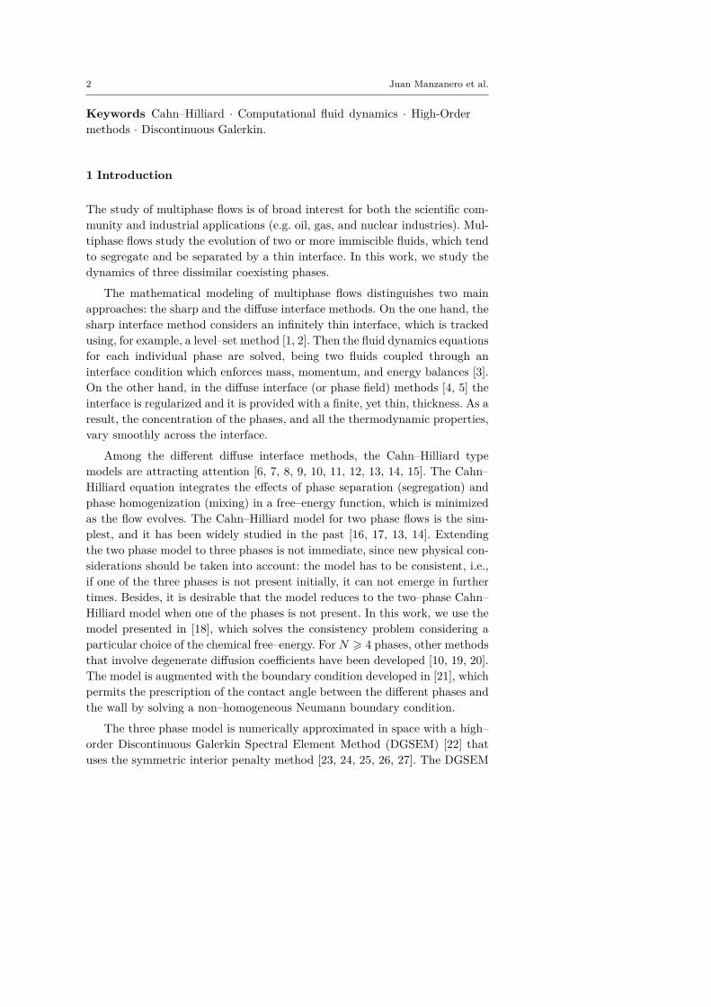
The L2 errors for both fluids concentration are represented in Fig. 2. The

Fig. 2 Convergence study: L2 errors as a function of the polynomial order N for the man-ufactured solution (50)

polynomial order ranges from N = 3 to N = 12. The error configuration isthe typical: a region with under–resolution in space (N < 11) where the so-lution converges as the polynomial order increases, and a region with under–resolution in time (N > 11), where the error stagnates. We see that the erroris higher for c1 than for c2, and that the behavior is not regular, with sys-tematically higher convergence rates for odd polynomial orders. We see thatfor c2, odd polynomial orders yield smaller errors than the theoretical linearbehavior, while for c1, on the contrary, even polynomial orders yield highererrors than expected. We do not have an answer for this behavior, althoughit has been seen in other works that particular choices of the manufacturedsolution might lead to this even–odd phenomena [49, 37, 13].


4.2 Captive bubble simulation

In the second test, we study a bubble (of phase 3) immersed in two layersof the other two phases. As a result of the interface tension, the equilibriumis reached when the angles between the different phases at the triple point(c1 = c2 = c3 = 1/3) satisfy [18],

σ23

cos θ1= σ13

cos θ2= σ12

cos θ3. (52)

We consider the three different cases for the interface tension coefficients de-scribed in [18], which are summarized in Table 2 along with the equilibriumtriple point angles computed with (52). For all the three cases, the initial

Table 2 Captive bubble simulation: interface tension coefficient values and equilibriumangles studied

Test σ12 σ13 σ23 θ1 θ2 θ31 1 0.8 1.4 130.54 111.80 117.662 1 1 1 120 120 1203 1 0.6 0.6 130.54 111.80 117.66

condition is

c1(x, y, 0) = 12

(1 + tanh

(2min(‖x‖ − 0.1, y)

ε

)),

c2(x, y, 0) = 12

(1− tanh

(2max(0.1− ‖x‖, y)

ε

)),

(53)

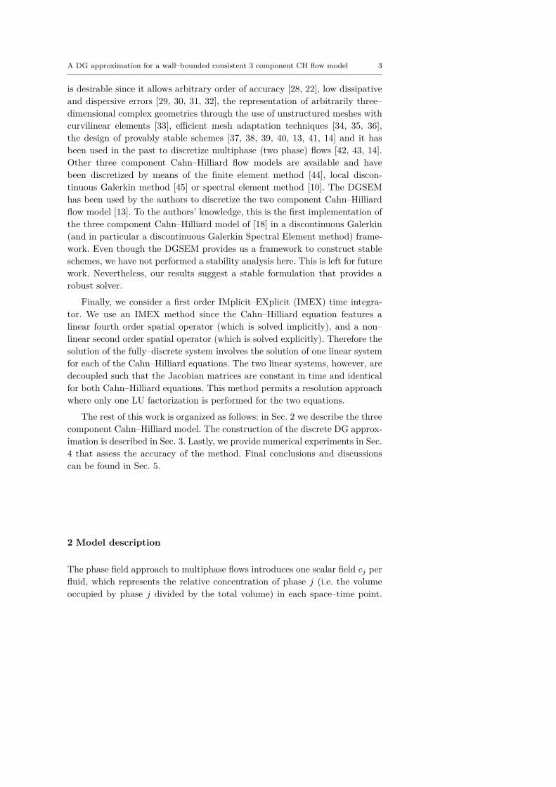
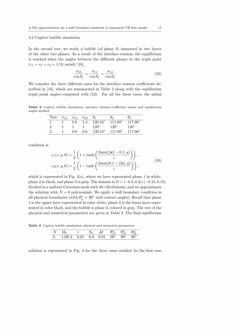
which is represented in Fig. 3(a), where we have represented phase 1 in white,phase 2 in black, and phase 3 in gray. The domain isΩ = [−0.3, 0.3]×[−0.15, 0.15],divided in a uniform Cartesian mesh with 40×20 elements, and we approximatethe solution with N = 8 polynomials. We apply a wall boundary condition inall physical boundaries (with θwij = 90 wall contact angles). Recall that phase1 is the upper layer represented in color white, phase 2 is the lower layer repre-sented in color black, and the bubble is phase 3, colored in gray. The rest of thephysical and numerical parameters are given in Table 3. The final equilibrium

Table 3 Captive bubble simulation: physical and numerical parameters

N M0 ε S0 ∆t θw12 θw13 θw238 1.0E-4 0.01 8.0 0.01 90 90 90

solution is represented in Fig. 3 for the three cases studied. In the first case


(a) Initial condition (b) σ12 = 1, σ13 = 0.8, σ23 = 1.4

(c) σ12 = 1, σ13 = 1, σ23 = 1 (d) σ12 = 1, σ13 = 0.6, σ23 = 0.6

Fig. 3 Captive bubble simulation:

(Fig. 3(b)), given σ13 < σ23, the bubble rises from the initial position, as aresult of a higher interfacial tension of the bubble with phase 2 than comparedwith phase 1. In the other two cases (Figs. 3(c),3(d)), the conditions are sym-metric as σ13 = σ23, and we obtain a lenticular shape. We observe that whenσ12 > σ13 = σ23, the lens flattens. These results are in agreement with thosein [18]. Moreover, in the right triple point, we have represented with red linesthe angles estimated from the theoretical equilibrium configuration (52). Weconfirm that all three solutions show a good agreement with the theory (52)and with the reference [18].

4.3 Wall contact angle simulation

The last two–dimensional test case assesses the exactness of the wall contactangle boundary condition (21). We consider two bubbles of phases 1 and 2 incontact with the inferior and immersed in phase 3. We specify the equilibriumwall contact angles θw13 and θw23, and compute the remaining third angle θw12from (20). We maintain the same domain and mesh (with polynomial order


N = 8) used for the captive bubble simulation. The new initial condition is

c1(x, y, 0) = 12 −

12 tanh

2(√

(x+ 0.05)2 + (y + 0.15)2 − 0.1)

ε

,

c2(x, y, 0) = 12 −

12 tanh

2(√

(x− 0.1)2 + (y + 0.12)2 − 0.1)

ε

,

c2 (x, y, 0) = min (c2(x, y, 0), 1− c1 (x, y, 0)) ,

(54)

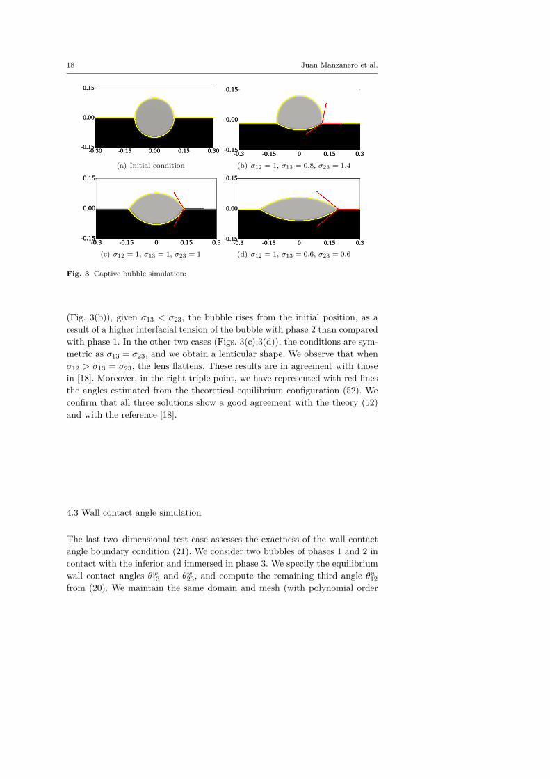
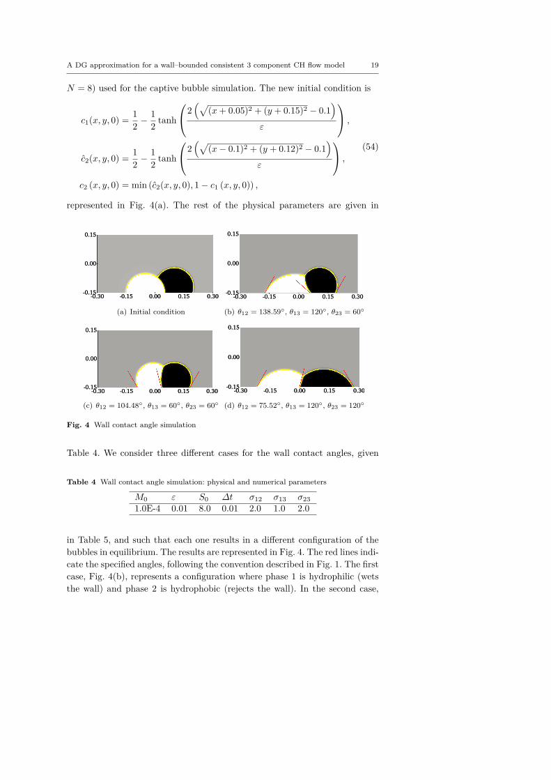
represented in Fig. 4(a). The rest of the physical parameters are given in

(a) Initial condition (b) θ12 = 138.59, θ13 = 120, θ23 = 60

(c) θ12 = 104.48, θ13 = 60, θ23 = 60 (d) θ12 = 75.52, θ13 = 120, θ23 = 120

Fig. 4 Wall contact angle simulation

Table 4. We consider three different cases for the wall contact angles, given

Table 4 Wall contact angle simulation: physical and numerical parameters

M0 ε S0 ∆t σ12 σ13 σ231.0E-4 0.01 8.0 0.01 2.0 1.0 2.0

in Table 5, and such that each one results in a different configuration of thebubbles in equilibrium. The results are represented in Fig. 4. The red lines indi-cate the specified angles, following the convention described in Fig. 1. The firstcase, Fig. 4(b), represents a configuration where phase 1 is hydrophilic (wetsthe wall) and phase 2 is hydrophobic (rejects the wall). In the second case,


Table 5 Wall contact angle simulation: wall contact angles specified for the three testsstudied

Test θw12 θw13 θw231 138.60 120 602 104.48 60 603 75.52 120 120

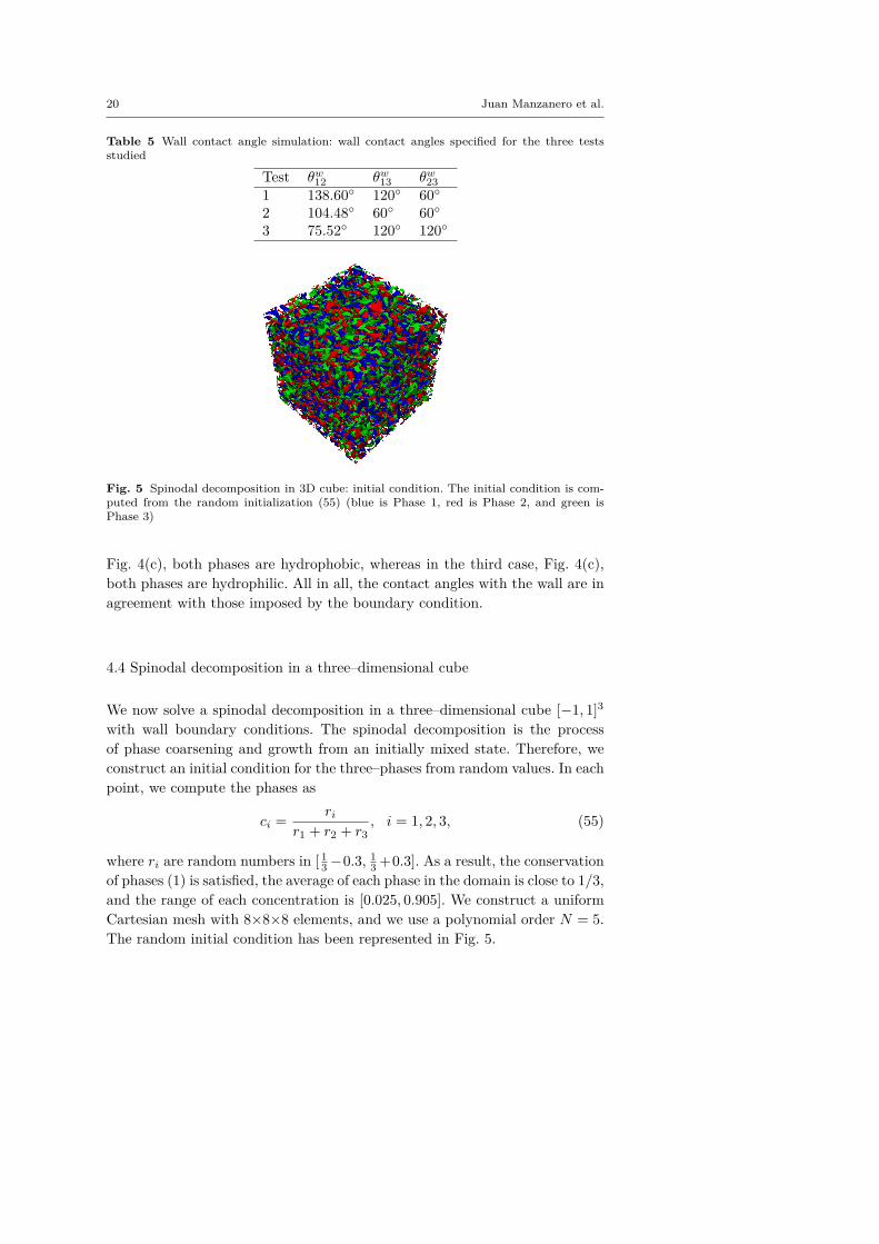
Fig. 5 Spinodal decomposition in 3D cube: initial condition. The initial condition is com-puted from the random initialization (55) (blue is Phase 1, red is Phase 2, and green isPhase 3)

Fig. 4(c), both phases are hydrophobic, whereas in the third case, Fig. 4(c),both phases are hydrophilic. All in all, the contact angles with the wall are inagreement with those imposed by the boundary condition.

4.4 Spinodal decomposition in a three–dimensional cube

We now solve a spinodal decomposition in a three–dimensional cube [−1, 1]3with wall boundary conditions. The spinodal decomposition is the processof phase coarsening and growth from an initially mixed state. Therefore, weconstruct an initial condition for the three–phases from random values. In eachpoint, we compute the phases as

ci = rir1 + r2 + r3

, i = 1, 2, 3, (55)

where ri are random numbers in [ 13−0.3, 1

3 +0.3]. As a result, the conservationof phases (1) is satisfied, the average of each phase in the domain is close to 1/3,and the range of each concentration is [0.025, 0.905]. We construct a uniformCartesian mesh with 8×8×8 elements, and we use a polynomial order N = 5.The random initial condition has been represented in Fig. 5.


Table 6 Spinodal decomposition in 3D cube: physical and numerical parameters

Test N M0 ε S0 ∆t σ12 σ13 σ23 θw12 θw13 θw231 5 1.0 0.10 8.0 10−3 1.0 1.0 1.0 90 90 902 5 1.0 0.10 8.0 10−3 1.0 1.0 1.0 170 90 10

(a) t = 0.02 (b) t = 0.1 (c) t = 0.2

(d) t = 0.5 (e) t = 1.0 (f) t = 10.0

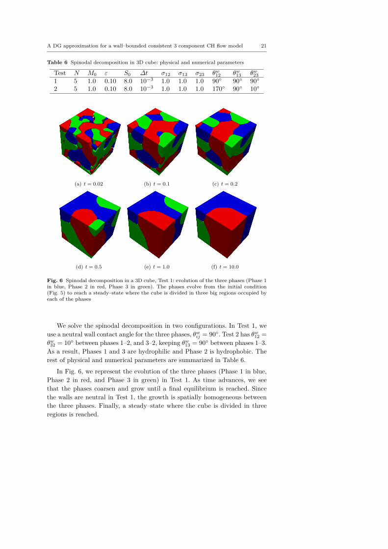
Fig. 6 Spinodal decomposition in a 3D cube, Test 1: evolution of the three phases (Phase 1in blue, Phase 2 in red, Phase 3 in green). The phases evolve from the initial condition(Fig. 5) to reach a steady–state where the cube is divided in three big regions occupied byeach of the phases

We solve the spinodal decomposition in two configurations. In Test 1, weuse a neutral wall contact angle for the three phases, θwij = 90. Test 2 has θw12 =θw32 = 10 between phases 1–2, and 3–2, keeping θw13 = 90 between phases 1–3.As a result, Phases 1 and 3 are hydrophilic and Phase 2 is hydrophobic. Therest of physical and numerical parameters are summarized in Table 6.

In Fig. 6, we represent the evolution of the three phases (Phase 1 in blue,Phase 2 in red, and Phase 3 in green) in Test 1. As time advances, we seethat the phases coarsen and grow until a final equilibrium is reached. Sincethe walls are neutral in Test 1, the growth is spatially homogeneous betweenthe three phases. Finally, a steady–state where the cube is divided in threeregions is reached.


(a) t = 0.02 (b) t = 0.1 (c) t = 0.2

(d) t = 0.5 (e) t = 1.0 (f) t = 10.0

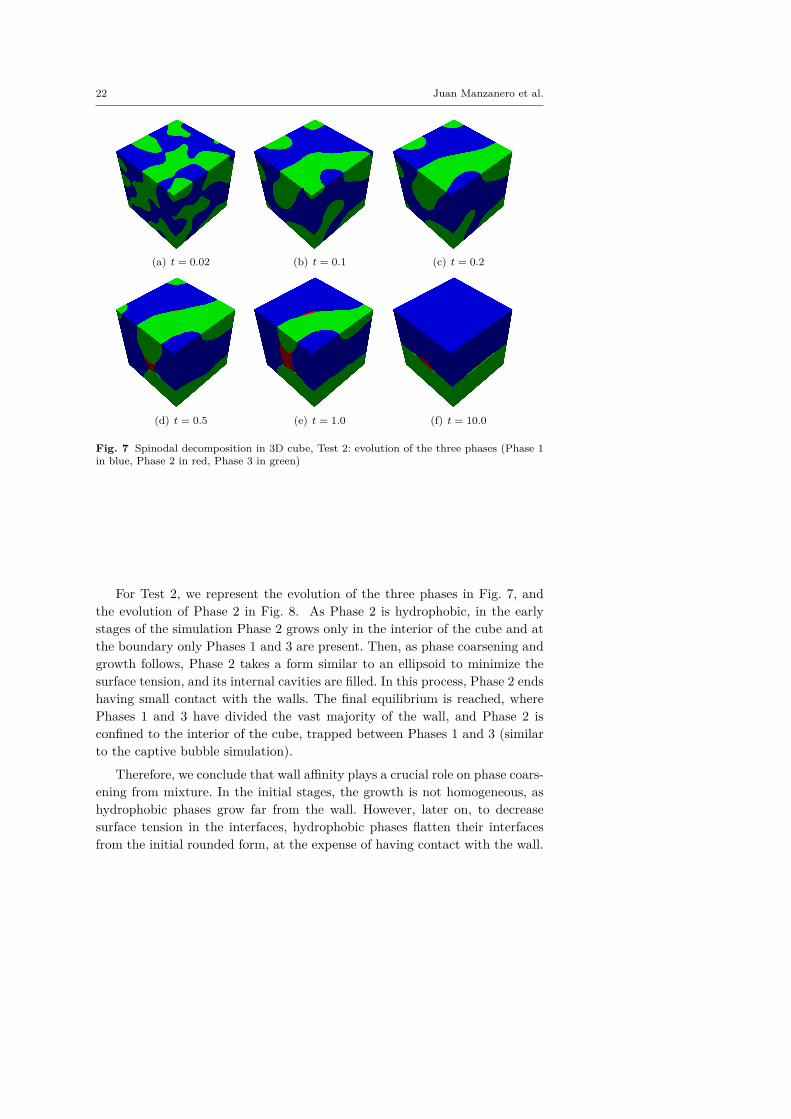
Fig. 7 Spinodal decomposition in 3D cube, Test 2: evolution of the three phases (Phase 1in blue, Phase 2 in red, Phase 3 in green)

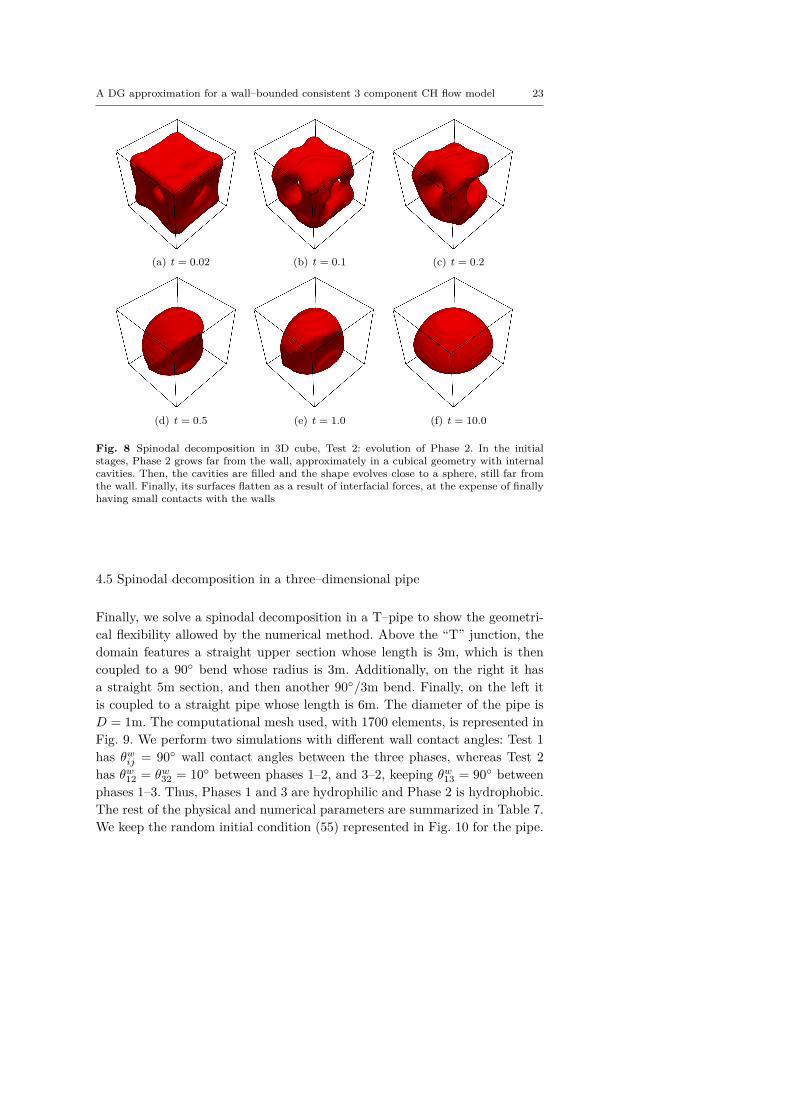
For Test 2, we represent the evolution of the three phases in Fig. 7, andthe evolution of Phase 2 in Fig. 8. As Phase 2 is hydrophobic, in the earlystages of the simulation Phase 2 grows only in the interior of the cube and atthe boundary only Phases 1 and 3 are present. Then, as phase coarsening andgrowth follows, Phase 2 takes a form similar to an ellipsoid to minimize thesurface tension, and its internal cavities are filled. In this process, Phase 2 endshaving small contact with the walls. The final equilibrium is reached, wherePhases 1 and 3 have divided the vast majority of the wall, and Phase 2 isconfined to the interior of the cube, trapped between Phases 1 and 3 (similarto the captive bubble simulation).

Therefore, we conclude that wall affinity plays a crucial role on phase coars-ening from mixture. In the initial stages, the growth is not homogeneous, ashydrophobic phases grow far from the wall. However, later on, to decreasesurface tension in the interfaces, hydrophobic phases flatten their interfacesfrom the initial rounded form, at the expense of having contact with the wall.


(a) t = 0.02 (b) t = 0.1 (c) t = 0.2

(d) t = 0.5 (e) t = 1.0 (f) t = 10.0

Fig. 8 Spinodal decomposition in 3D cube, Test 2: evolution of Phase 2. In the initialstages, Phase 2 grows far from the wall, approximately in a cubical geometry with internalcavities. Then, the cavities are filled and the shape evolves close to a sphere, still far fromthe wall. Finally, its surfaces flatten as a result of interfacial forces, at the expense of finallyhaving small contacts with the walls

4.5 Spinodal decomposition in a three–dimensional pipe

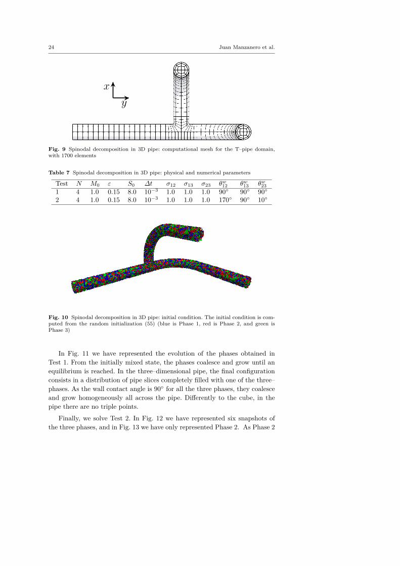
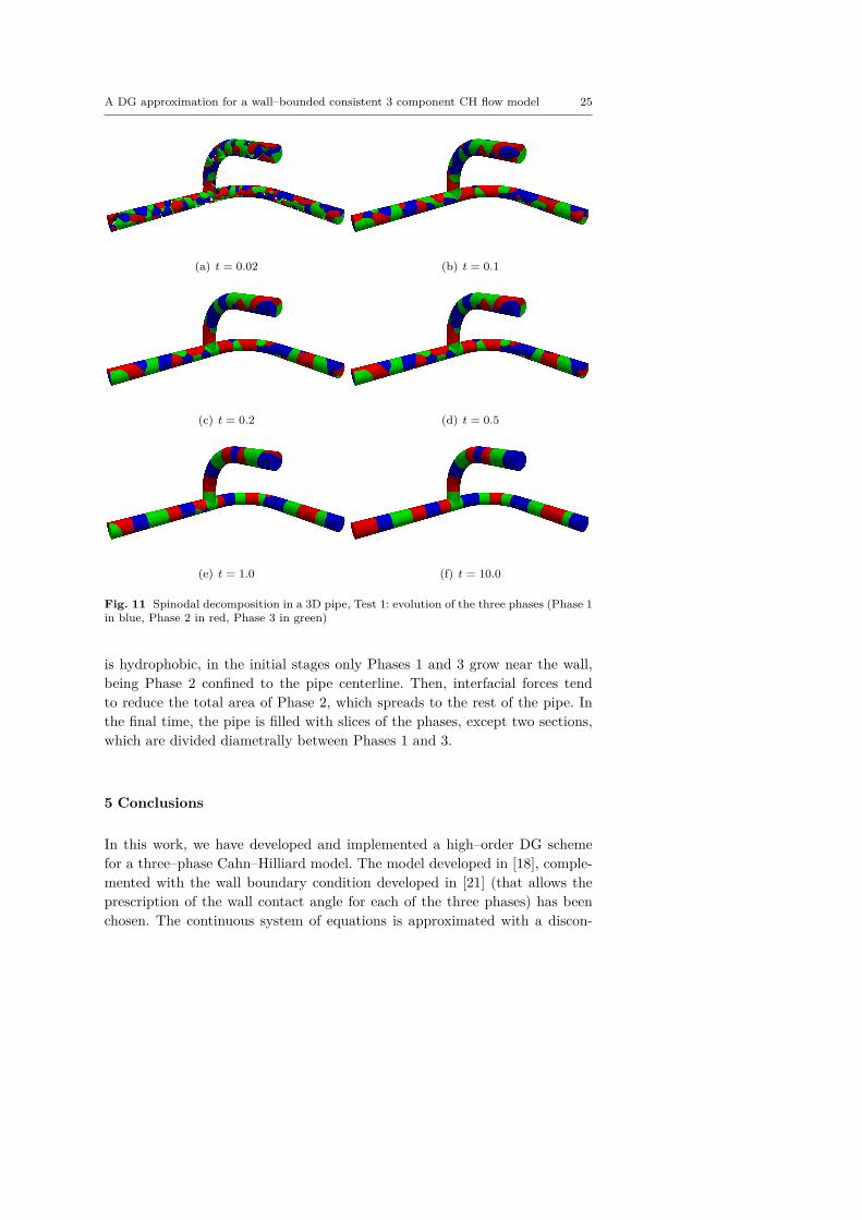
Finally, we solve a spinodal decomposition in a T–pipe to show the geometri-cal flexibility allowed by the numerical method. Above the “T” junction, thedomain features a straight upper section whose length is 3m, which is thencoupled to a 90 bend whose radius is 3m. Additionally, on the right it hasa straight 5m section, and then another 90/3m bend. Finally, on the left itis coupled to a straight pipe whose length is 6m. The diameter of the pipe isD = 1m. The computational mesh used, with 1700 elements, is represented inFig. 9. We perform two simulations with different wall contact angles: Test 1has θwij = 90 wall contact angles between the three phases, whereas Test 2has θw12 = θw32 = 10 between phases 1–2, and 3–2, keeping θw13 = 90 betweenphases 1–3. Thus, Phases 1 and 3 are hydrophilic and Phase 2 is hydrophobic.The rest of the physical and numerical parameters are summarized in Table 7.We keep the random initial condition (55) represented in Fig. 10 for the pipe.


x

y

Fig. 9 Spinodal decomposition in 3D pipe: computational mesh for the T–pipe domain,with 1700 elements

Table 7 Spinodal decomposition in 3D pipe: physical and numerical parameters

Test N M0 ε S0 ∆t σ12 σ13 σ23 θw12 θw13 θw231 4 1.0 0.15 8.0 10−3 1.0 1.0 1.0 90 90 902 4 1.0 0.15 8.0 10−3 1.0 1.0 1.0 170 90 10

Fig. 10 Spinodal decomposition in 3D pipe: initial condition. The initial condition is com-puted from the random initialization (55) (blue is Phase 1, red is Phase 2, and green isPhase 3)

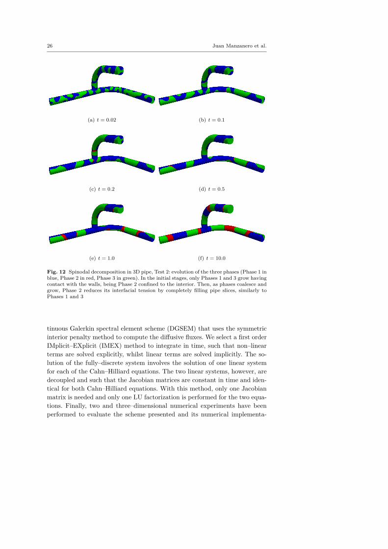
In Fig. 11 we have represented the evolution of the phases obtained inTest 1. From the initially mixed state, the phases coalesce and grow until anequilibrium is reached. In the three–dimensional pipe, the final configurationconsists in a distribution of pipe slices completely filled with one of the three–phases. As the wall contact angle is 90 for all the three phases, they coalesceand grow homogeneously all across the pipe. Differently to the cube, in thepipe there are no triple points.

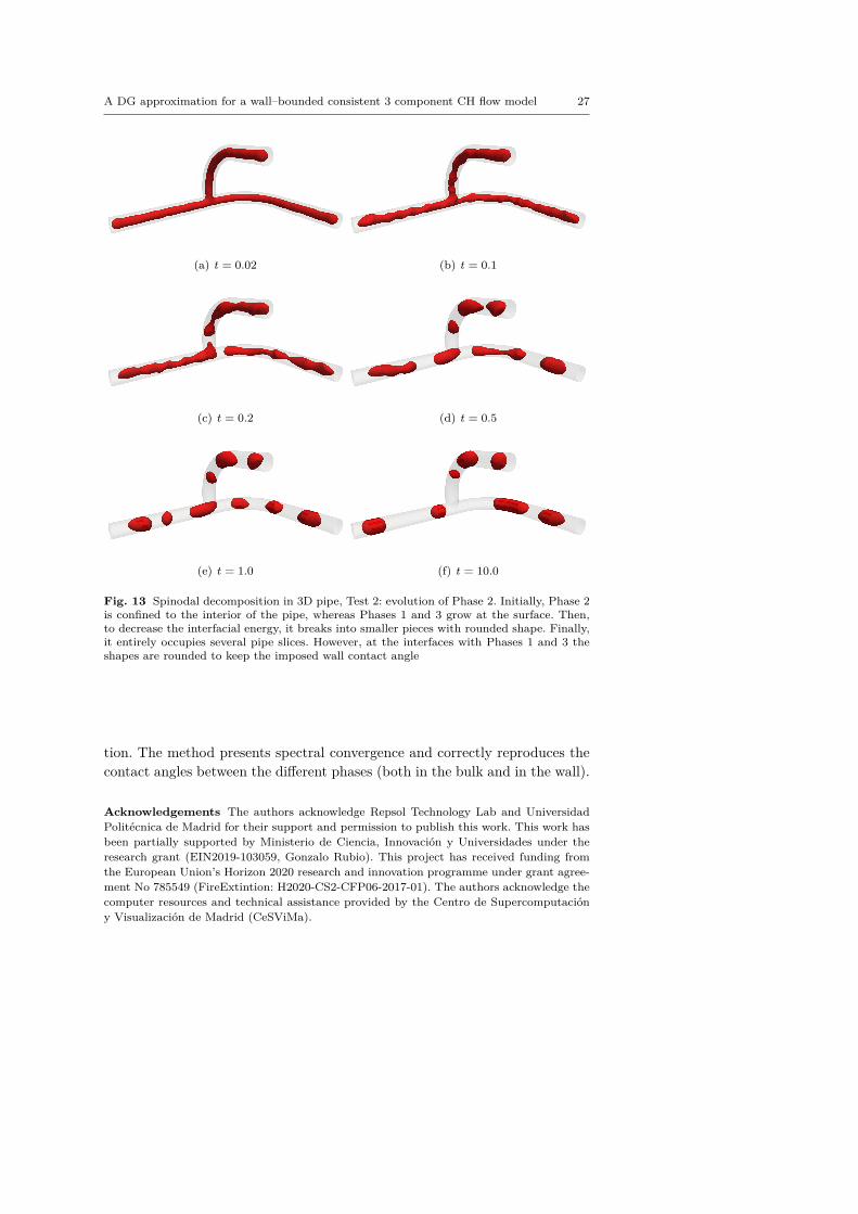
Finally, we solve Test 2. In Fig. 12 we have represented six snapshots ofthe three phases, and in Fig. 13 we have only represented Phase 2. As Phase 2


(a) t = 0.02 (b) t = 0.1

(c) t = 0.2 (d) t = 0.5

(e) t = 1.0 (f) t = 10.0

Fig. 11 Spinodal decomposition in a 3D pipe, Test 1: evolution of the three phases (Phase 1in blue, Phase 2 in red, Phase 3 in green)

is hydrophobic, in the initial stages only Phases 1 and 3 grow near the wall,being Phase 2 confined to the pipe centerline. Then, interfacial forces tendto reduce the total area of Phase 2, which spreads to the rest of the pipe. Inthe final time, the pipe is filled with slices of the phases, except two sections,which are divided diametrally between Phases 1 and 3.

5 Conclusions

In this work, we have developed and implemented a high–order DG schemefor a three–phase Cahn–Hilliard model. The model developed in [18], comple-mented with the wall boundary condition developed in [21] (that allows theprescription of the wall contact angle for each of the three phases) has beenchosen. The continuous system of equations is approximated with a discon-


(a) t = 0.02 (b) t = 0.1

(c) t = 0.2 (d) t = 0.5

(e) t = 1.0 (f) t = 10.0

Fig. 12 Spinodal decomposition in 3D pipe, Test 2: evolution of the three phases (Phase 1 inblue, Phase 2 in red, Phase 3 in green). In the initial stages, only Phases 1 and 3 grow havingcontact with the walls, being Phase 2 confined to the interior. Then, as phases coalesce andgrow, Phase 2 reduces its interfacial tension by completely filling pipe slices, similarly toPhases 1 and 3

tinuous Galerkin spectral element scheme (DGSEM) that uses the symmetricinterior penalty method to compute the diffusive fluxes. We select a first orderIMplicit–EXplicit (IMEX) method to integrate in time, such that non–linearterms are solved explicitly, whilst linear terms are solved implicitly. The so-lution of the fully–discrete system involves the solution of one linear systemfor each of the Cahn–Hilliard equations. The two linear systems, however, aredecoupled and such that the Jacobian matrices are constant in time and iden-tical for both Cahn–Hilliard equations. With this method, only one Jacobianmatrix is needed and only one LU factorization is performed for the two equa-tions. Finally, two and three–dimensional numerical experiments have beenperformed to evaluate the scheme presented and its numerical implementa-


(a) t = 0.02 (b) t = 0.1

(c) t = 0.2 (d) t = 0.5

(e) t = 1.0 (f) t = 10.0

Fig. 13 Spinodal decomposition in 3D pipe, Test 2: evolution of Phase 2. Initially, Phase 2is confined to the interior of the pipe, whereas Phases 1 and 3 grow at the surface. Then,to decrease the interfacial energy, it breaks into smaller pieces with rounded shape. Finally,it entirely occupies several pipe slices. However, at the interfaces with Phases 1 and 3 theshapes are rounded to keep the imposed wall contact angle

tion. The method presents spectral convergence and correctly reproduces thecontact angles between the different phases (both in the bulk and in the wall).

Acknowledgements The authors acknowledge Repsol Technology Lab and UniversidadPolitecnica de Madrid for their support and permission to publish this work. This work hasbeen partially supported by Ministerio de Ciencia, Innovacion y Universidades under theresearch grant (EIN2019-103059, Gonzalo Rubio). This project has received funding fromthe European Union’s Horizon 2020 research and innovation programme under grant agree-ment No 785549 (FireExtintion: H2020-CS2-CFP06-2017-01). The authors acknowledge thecomputer resources and technical assistance provided by the Centro de Supercomputaciony Visualizacion de Madrid (CeSViMa).


References

1. M. Sussman, P. Smereka, S. Osher, A level set approach for computing solutions toincompressible two-phase flow, Journal of Computational physics 114 (1) (1994) 146–159 (1994).

2. D. Adalsteinsson, J. A. Sethian, A fast level set method for propagating interfaces,Journal of computational physics 118 (2) (1995) 269–277 (1995).

3. S. Van der Pijl, A. Segal, C. Vuik, P. Wesseling, A mass-conserving level-set methodfor modelling of multi-phase flows, International journal for numerical methods in fluids47 (4) (2005) 339–361 (2005).

4. J. W. Cahn, J. E. Hilliard, Free energy of a nonuniform system. I. Interfacial free energy,The Journal of chemical physics 28 (2) (1958) 258–267 (1958).

5. J. W. Cahn, J. E. Hilliard, Free energy of a nonuniform system. III. Nucleation in a two-component incompressible fluid, The Journal of chemical physics 31 (3) (1959) 688–699(1959).

6. C. M. Elliott, H. Garcke, On the Cahn–Hilliard equation with degenerate mobility, Siamjournal on mathematical analysis 27 (2) (1996) 404–423 (1996).

7. J. Lowengrub, L. Truskinovsky, Quasi–incompressible Cahn–Hilliard fluids and topolog-ical transitions, Proceedings of the Royal Society of London. Series A: Mathematical,Physical and Engineering Sciences 454 (1978) (1998) 2617–2654 (1998).

8. H. Gomez, V. M. Calo, Y. Bazilevs, T. J. Hughes, Isogeometric analysis of the Cahn–Hilliard phase-field model, Computer methods in applied mechanics and engineering197 (49-50) (2008) 4333–4352 (2008).

9. J. Shen, X. Yang, Numerical approximations of Allen-Cahn and Cahn-Hilliard equa-tions, Discrete Contin. Dyn. Syst 28 (4) (2010) 1669–1691 (2010).

10. S. Dong, An efficient algorithm for incompressible N-phase flows, Journal of Computa-tional Physics 276 (2014) 691–728 (2014).

11. S. Dong, Wall-bounded multiphase flows of N immiscible incompressible fluids: Con-sistency and contact-angle boundary condition, Journal of Computational Physics 338(2017) 21–67 (2017).

12. S. Gomez-Alvarez, A. Rivero-Jimenez, G. Rubio, J. Manzanero, C. Redondo, et al.,Novel Coupled Cahn-Hilliard Navier-Stokes Solver for the Evaluation of Oil and GasMultiphase Flow, in: BHR 19th International Conference on Multiphase ProductionTechnology, BHR Group, 2019 (2019).

13. J. Manzanero, G. Rubio, D. A. Kopriva, E. Ferrer, E. Valero, A free-energy stablenodal discontinuous Galerkin approximation with summation-by-parts property for theCahn-Hilliard equation, Journal of Computational Physics 403 (2020) 109072 (2020).

14. J. Manzanero, G. Rubio, D. A. Kopriva, E. Ferrer, E. Valero, Entropy-stable discontin-uous Galerkin approximation with summation-by-parts property for the incompressibleNavier-Stokes/Cahn-Hilliard system, Journal of Computational Physics (2020) 109363(2020).

15. J. Manzanero, C. Redondo, G. Rubio, E. Ferrer, E. Valero, S. Gomez-Alvarez, A. Rivero,A high–order discontinuous Galerkin solver for multiphase flows, in: Spectral andHigh Order Methods for Partial Differential Equations ICOSAHOM 2018 (accepted),Springer, 2020 (2020).

16. Y. Xia, Y. Xu, C.-W. Shu, Application of the local discontinuous Galerkin methodfor the Allen-Cahn/Cahn-Hilliard system, Communications in Computational Physics5 (2-4) (2009) 821–835 (2009).

17. J. Shen, X. Yang, Energy stable schemes for Cahn-Hilliard phase-field model of two-phase incompressible flows, Chinese Annals of Mathematics, Series B 31 (5) (2010)743–758 (2010).


18. F. Boyer, C. Lapuerta, Study of a three component Cahn-Hilliard flow model, ESAIM:Mathematical Modelling and Numerical Analysis 40 (4) (2006) 653–687 (2006).

19. F. Boyer, S. Minjeaud, Hierarchy of consistent N-component Cahn–Hilliard systems,Mathematical Models and Methods in Applied Sciences 24 (14) (2014) 2885–2928(2014).

20. S. Dong, Multiphase flows of N immiscible incompressible fluids: A reduction-consistentand thermodynamically-consistent formulation and associated algorithm, Journal ofComputational Physics 361 (2018) 1–49 (2018).

21. Y. Shi, X.-P. Wang, Modeling and simulation of dynamics of three-component flowson solid surface, Japan Journal of Industrial and Applied Mathematics 31 (3) (2014)611–631 (2014).

22. D.A. Kopriva, Implementing spectral methods for partial differential equations, SpringerNetherlands, 2009 (2009).

23. M. F. Wheeler, An elliptic collocation-finite element method with interior penalties,SIAM Journal on Numerical Analysis 15 (1) (1978) 152–161 (1978).

24. E. Ferrer and R.H.J. Willden, A high order discontinuous Galerkin finite element solverfor the incompressible Navier–Stokes equations, Computers & Fluids 46 (1) (2011) 224–230 (2011).

25. E. Ferrer and R. H.J. Willden, A high order discontinuous Galerkin - Fourier incom-pressible 3D Navier-Stokes solver with rotating sliding meshes, Journal of Computa-tional Physics 231 (21) (2012) 7037–7056 (2012).

26. E. Ferrer, An interior penalty stabilised incompressible Discontinuous Galerkin - Fouriersolver for implicit Large Eddy Simulations, Journal of Computational Physics 348 (2017)754–775 (2017).

27. J. Manzanero, A. M. Rueda-Ramırez, G. Rubio, E. Ferrer, The Bassi Rebay 1 scheme isa special case of the symmetric interior penalty formulation for discontinuous Galerkindiscretisations with Gauss–Lobatto points, Journal of Computational Physics 363 (2018)1–10 (2018).

28. J. S. Hesthaven, T. Warburton, Nodal discontinuous Galerkin methods: algorithms,analysis, and applications, Springer Science & Business Media, 2007 (2007).

29. G. Gassner, D. A. Kopriva, A comparison of the dispersion and dissipation errors ofGauss and Gauss–Lobatto discontinuous Galerkin spectral element methods, SIAMJournal on Scientific Computing 33 (5) (2011) 2560–2579 (2011).

30. R. C. Moura, S. J. Sherwin, J. Peiro, Linear dispersion–diffusion analysis and its applica-tion to under-resolved turbulence simulations using discontinuous Galerkin spectral/hpmethods, Journal of Computational Physics 298 (2015) 695–710 (2015).

31. J. Manzanero, G. Rubio, E. Ferrer, E. Valero, Dispersion-dissipation analysis for ad-vection problems with nonconstant coefficients: Applications to discontinuous Galerkinformulations, SIAM Journal on Scientific Computing 40 (2) (2018) A747–A768 (2018).

32. J. Manzanero, E. Ferrer, G. Rubio, E. Valero, Design of a smagorinsky spectral vanishingviscosity turbulence model for discontinuous Galerkin methods, Computers & Fluids(2020) 104440 (2020).

33. D. A. Kopriva, Metric identities and the discontinuous spectral element method oncurvilinear meshes, Journal of Scientific Computing 26 (3) (2006) 301 (2006).

34. M. Kompenhans, G. Rubio, E. Ferrer, and E. Valero, Comparisons of p–adaptationstrategies based on truncation– and discretisation–errors for high order discontinuousGalerkin methods, Computers & Fluids 139 (2016) 36 – 46, 13th USNCCM Inter-national Symposium of High-Order Methods for Computational Fluid Dynamics - Aspecial issue dedicated to the 60th birthday of Professor David Kopriva (2016).

35. M. Kompenhans, G. Rubio, E. Ferrer, and E. Valero, Adaptation strategies for high orderdiscontinuous Galerkin methods based on tau-estimation, Journal of ComputationalPhysics 306 (2016) 216 – 236 (2016).


36. A. M. Rueda-Ramırez, J. Manzanero, E. Ferrer, G. Rubio, E. Valero, A p-multigridstrategy with anisotropic p-adaptation based on truncation errors for high-order dis-continuous Galerkin methods, Journal of Computational Physics 378 (2019) 209–233(2019).

37. G. J. Gassner, A. R. Winters, D. A. Kopriva, Split form nodal discontinuous Galerkinschemes with summation-by-parts property for the compressible Euler equations, Jour-nal of Computational Physics 327 (2016) 39–66 (2016).

38. A. R. Winters, G. J. Gassner, Affordable, entropy conserving and entropy stable fluxfunctions for the ideal MHD equations, Journal of Computational Physics 304 (2016)72–108 (2016).

39. J. Manzanero, G. Rubio, E. Ferrer, E. Valero, D. A. Kopriva, Insights on aliasing driveninstabilities for advection equations with application to Gauss–Lobatto discontinuousGalerkin methods, Journal of Scientific Computing 75 (3) (2018) 1262–1281 (2018).

40. G. J. Gassner, A. R. Winters, F. J. Hindenlang, D. A. Kopriva, The BR1 scheme isstable for the compressible Navier–Stokes equations, Journal of Scientific Computing77 (1) (2018) 154–200 (2018).

41. J. Manzanero, G. Rubio, D. A. Kopriva, E. Ferrer, E. Valero, An entropy–stable discon-tinuous Galerkin approximation for the incompressible Navier–Stokes equations withvariable density and artificial compressibility, Journal of Computational Physics 408(2020) 109241 (2020).

42. F. Fraysse, C. Redondo, G. Rubio, E. Valero, Upwind methods for the Baer–Nunziatoequations and higher-order reconstruction using artificial viscosity, Journal of Compu-tational Physics 326 (2016) 805–827 (2016).

43. C. Redondo, F. Fraysse, G. Rubio, E. Valero, Artificial Viscosity Discontinuous GalerkinSpectral Element Method for the Baer-Nunziato Equations, in: Spectral and High OrderMethods for Partial Differential Equations ICOSAHOM 2016, Springer, 2017, pp. 613–625 (2017).

44. F. Boyer, S. Minjeaud, Numerical schemes for a three component Cahn-Hilliard model,ESAIM: Mathematical Modelling and Numerical Analysis 45 (4) (2011) 697–738 (2011).

45. Y. Xia, Y. Xu, C.-W. Shu, Local discontinuous Galerkin methods for the Cahn–Hilliardtype equations, Journal of Computational Physics 227 (1) (2007) 472–491 (2007).

46. S. Dong, On imposing dynamic contact-angle boundary conditions for wall-boundedliquid–gas flows, Computer Methods in Applied Mechanics and Engineering 247 (2012)179–200 (2012).

47. Y. Shi, X.-P. Wang, Modeling and simulation of dynamics of three-component flowson solid surface, Japan Journal of Industrial and Applied Mathematics 31 (3) (2014)611–631 (2014).

48. K. Shahbazi, Short note: An explicit expression for the penalty parameter of the interiorpenalty method, Journal of Computational Physics 205 (2) (2005) 401–407 (May 2005).

49. G. Rubio, F. Fraysse, J. De Vicente, E. Valero, The estimation of truncation error by τ -estimation for Chebyshev spectral collocation method, Journal of Scientific Computing57 (1) (2013) 146–173 (2013).

Documents

A discontinuous Galerkin approximation for a wall–bounded