Embed Size (px)
Citation preview
A DEVELOPED SMART TECHNIQUE TO PREDICT MINIMUM MISCIBLEPRESSURE—EOR IMPLICATIONS
Sohrab Zendehboudi,1* Mohammad Ali Ahmadi,2 Alireza Bahadori,3 Ali Shafiei4 and Tayfun Babadagli5
1. Department of Chemical Engineering, University of Waterloo, Waterloo, Ontario, Canada, N2L 3G1
2. Faculty of Petroleum Engineering, Petroleum University of Technology, Ahwaz, Iran
3. School of Environment, Science and Engineering, Southern Cross University, Lismore, New South Wales, Australia
4. Department of Earth and Environmental Sciences, University of Waterloo, Waterloo, Ontario, Canada
5. Department of Civil and Environmental Engineering, School of Mining and Petroleum Engineering, University of Alberta, Edmonton,Alberta, Canada
Miscible gas injection (MGI) processes such as miscible CO2 flooding have been in use as attractive EOR options, especially in conventional oilreserves. Optimal design of MGI is strongly dependent on parameters such as gas–oil minimum miscibility pressure (MMP), which is normallydetermined through expensive and time-consuming laboratory tests. Thus, developing a fast and reliable technique to predict gas–oil MMP isinevitable. To address this issue, a smart model is developed in this paper to forecast gas–oil MMP on the basis of a feed-forward artificial neuralnetwork (FF-ANN) combined with particle swarm optimisation (PSO). The MMP of a reservoir fluid was considered as a function of reservoirtemperature and the compositions of oil and injected gas in the proposed model. Results of this study indicate that reservoir temperature amongthe input parameters selected for the PSO–ANN has the greatest impact on MMP value. The developed PSO–ANN model was examined usingexperimental data, and a reasonable match was attained showing a good potential for the proposed predictive tools in estimation of gas–oilMMP. Compared with other available methods, the proposed model is capable of forecasting oil–gas MMP more accurately in wide ranges ofthermodynamic and process conditions. All predictive models used other than the PSO–ANN model failed in providing a good estimate of theoil–gas MMP of the hydrocarbon mixtures in Azadegan oilfield, Iran.
Keywords: minimum miscible pressure, smart technique, experimental study, miscible gas flooding, EOR, optimised neural network
INTRODUCTION
Gas injection processes, particularly CO2 flooding, havebeen in use as attractive and benign enhanced oil recov-ery (EOR) options in conventional oil reserves, leading
to additional oil recovery of over 15% of the original oil inplace (OOIP).[1] Optimal design of the gas injection EOR projectsstrongly requires an accurate estimate of the gas–oil minimummiscibility pressure (MMP), since it controls the local displace-ment efficiency of the gas injected. MMP is usually defined asthe lowest pressure where oil and solvent develop miscibilitydynamically. In other words, the injected gas can reach dynamicmiscibility with the reservoir oil at this particular pressure.[2–6]
The displacement is assumed to be a piston-like process, con-sidering a 1D, two phase dispersion-free flow regime for thedisplacement process at the MMP. In this case, the oil produc-tion performance is expected to be 100% at 1 PV of the gasinjected.[2,4,5]
MMP prediction plays an important role in design and operationof gas injection projects including EOR and CO2 sequestration.Multiple contact miscibility between the oil and the injected gasis likely to occur at pressures higher than MMP. At displacementpressures higher than MMP, most favourable displacement effi-ciency for gas flooding processes is expected.[7] Several studieswere reported in the literature aiming at forecast of MMP forhydrocarbons and gases.[6–11]
Both high and low estimated values of MMP can lead to sometechnical issues. High values increase the operational costs sincemiscibility can develop through a vapourising process, a con-densing process or a combination of these. Low values of MMP
decrease the efficiency of the miscible displacement process andconsequently result in lower oil recoveries. Hence, the preciseassessment of the MMP can potentially result in major economicpayback.
MMP is a function of oil temperature, oil composition and gascomposition. Techniques commonly used for miscibility evalu-ation include slim tube displacement, rising bubble apparatus(RBA) and pressure composition diagrams. Slim tube displace-ments and RBA tests are the most common experiments indetermining the MMP.[5,12–15] Multiple-contact experiments (mix-ing cell experiments) are a rapid and cheap alternative forslim-tube experiments when the miscibility mechanism is knownbeforehand (e.g. condensing or vapourising). However, theirinability in measuring the MMP for a condensing or vapourisingdrive limits their utilisation for EOR purposes considerably.[12]
The most widely used technique for MMP calculations is the tie-line method using the method of characteristics (MOC), which hasbeen implemented in commercial softwares.[5,12–15] However, theMMP calculation using MOC requires a reliable equation of state(EOS) fluid model. On the other hand, the EOS involves severalnumerical computations that need compositions of the mixturesin details. Collection of such data is both time-consuming and
∗Author to whom correspondence may be addressed.E-mail address: [email protected]. J. Chem. Eng. 9999:1–13, 2013© 2013 Canadian Society for Chemical EngineeringDOI 10.1002/cjce.21802Published online in Wiley Online Library(wileyonlinelibrary.com).
| VOLUME 9999, 2013 | | THE CANADIAN JOURNAL OF CHEMICAL ENGINEERING | 1 |

resource intensive. The success of EOS is mostly dependent on themixing rules selected for the equation and the range of PVT data.The MOC-based techniques that presume shocks between key tielines may result in obtaining wrong MMP values when the lengthsof the tie lines are not monotonic between each succeeding keytie line.[5,12–15]
Measurement of the interfacial tension of an oil-solvent mix-ture at reservoir condition can be used for MMP determinationas well.[15] Determining MMP using such time-consuming exper-imental techniques with high accuracy requires at least a weekof experimental work and is expensive.[14] Hence, development ofmathematical models with high precision to estimate the gas–oilMMP is inevitable in the absence of sufficient experimental datain early stages of EOR operations, and several attempts were madeto develop these types of alternative techniques.[13,16,17]
A number of correlations were introduced in the literature forprediction of gas–oil MMP. Holm and Josendal[9] proposed anadaptation for temperature to the Benham–Dowden–Kunzmanlcorrelation for enriched natural gas MMP. A correlation was alsointroduced by Orr and Silva[18] that requires a more complete dataon crude oil compositions. Riedel[19] suggested an extension toBenham et al.[20] approach considering compositional effects. Thelatter has <10% error in MMP prediction.[9,18–20]
Statistical models were also developed extensively in thisarea.[7,8,21–25] However, satisfying rigid assumptions such as sam-ple size, linearity and continuity are still major issues withstatistical models.
Artificial neural network (ANN) is considered as a potentiallyrobust technique in developing predictive models for the MMP.Two main steps in any ANN models are training/learning phaseand a cross validation phase. The first phase is to find a setof proper weights to minimise the error between the real andpredicted output. This step is fairly time-consuming. Having fin-ished this phase, the next task is to check the accuracy of themodel.[26–29] The main advantage of the ANN is its capability tohandle complex systems more effectively than traditional statis-tical methods. This is mainly because the ANN allows a largenumber of freedom or fitting parameters. Hence, the ANN systemcan be employed as a very powerful tool in various engineeringand science disciplines where there are numerous complicatedphenomena and processes.
In this paper, a new and more reliable model to determine thegas–oil MMP correlation using ANN with particle swarm opti-misation (PSO) is presented. PSO was applied here to optimisethe weights of feed-forward neural network. Furthermore, exper-imental data from an Iranian oilfield was used to evaluate theproposed approach against the common gas–oil MMP correla-tions and ANN. The accuracy of the PSO–ANN model was alsoexamined using experimental data available in literature and com-pared with MMP values calculated from the conventional neuralnetwork model and some well-known correlations (e.g. Ref.[8]).Results obtained from this study can be utilised in accurate estima-tion of MMP for EOR projects. This study shows that the PSO–ANNtechnique can offer a higher accuracy in estimating MMP com-pared to the empirical MMP correlations and the conventionalANN model when the oil field information is limited or/and theavailable data covers wide ranges of process and thermodynamicconditions.
MMP DETERMINATION TECHNIQUES
In this section, some of the techniques used for MMP determina-tion are described briefly.
Experimental Methods
Slim tube test
The slim tube test is one of the most commonly used techniquesand is widely accepted as a standard method for MMP deter-mination in petroleum industry.[5,12,18] In this test, a slim tubemade of stainless steel is packed with porous materials such asglass beads or sands.[5,12,18] The tube is initially saturated withoil. Gas is injected at the inlet of the tube to displace the oil atthe desired test temperature and pressure. Effluent from the tubeis collected and measured (recovery data). The recovery data areplotted versus the displacement pressures, and the recovery curveis recommended as a criterion to determine the pressure or fluidcompositions where dynamic miscibility occurs. The criteria usedby several researchers to find out the MMP from the oil recoverycurve are different. A generally used injection volume is 1.2 porevolumes. The recovery levels defining MMP vary from 90% to95%.[5,12,18] At this pressure, oil recovery versus pressure curveshows a sharp change in slope, in general. The MMP is conven-tionally termed as the lowest pressure at which basically all oilexisting for recovery can be displaced by the injected solvent.
Rising bubble apparatus
In this method, a glass tube is mounted in a high pressure visiblecell placed in a temperature controlled bath.[5,12,18] The MMP valueis determined from visual observations of variations in shape andappearance of the bubbles of the injected gas while going upwardthrough a thin column of crude oil. The pressure at which a risinggas bubble disappears in a column of oil is defined as the MMP.
Vanishing interfacial technique
Vanishing interfacial technique (VIT) has been developed byRao[30] as an improvement to slim tube and rising bubbletechniques in MMP determination. Although the experimentalapparatus is fairly complicated, the approach looks highly sim-ple in terms of its principles. VIT is based on the concept that theextent of IFT between the two phases goes to zero at the miscibil-ity condition.[30–33] The IFT between the injected gas and crude oilis measured at reservoir temperature and various pressures in thismethod. The MMP is then determined by extrapolating the plot ofIFT versus pressure at interfacial tension equal to zero.[30–33]
Core flooding
Core flooding tests are employed to determine MMP valueunder reservoir conditions. In this approach, pore throat sizesand presence of water phases are considered.[5,12,18] Hence, theresults seem more realistic compared with other common tech-niques. However, core flood tests are further expensive andtime-consuming, and core samples are not available all the timeduring the drilling of oil wells. In addition, it is not easy to obtain arepresentative core (e.g. uncertainties associated with the geologyof the reservoir) of adequate length with good quality to accom-plish the test runs. Short cores are usually scarce to create theconditions of multi-contact miscibility.
Mathematical Methods
Empirical correlations
Several empirical correlations were proposed in the literature forMMP estimation. The key factors contributing in the magnitudeof gas–oil MMP are formation temperature, oil compositions andthe components of injected gas.[33–39] For preliminary screeningpurposes, the correlations often give a fair initial guess dependingon the quality of the data used. In addition, they are inexpensive,
| 2 | THE CANADIAN JOURNAL OF CHEMICAL ENGINEERING | | VOLUME 9999, 2013 |
and simple calculations are needed to determine the MMP value.In general, the accuracy of such correlations depends on the com-position range in which these correlations were obtained. TheMMP correlations are classified into two groups, including pureCO2 and gas mixture containing hydrocarbons and CO2.
Analytical methods
The analytical methods are based on the PVT behaviour of fluids.The relevance of a selected EOS for phase behaviour prediction isstrongly dependent on the quality of data used and the mixturecomposition. Utilising analytical approaches is very common incompositional streamline simulation runs. Some of the availableanalytical methods include the equation of state model, ternarydiagram, the tie-line algorithm, the C/V mechanism, single mix-ing cell algorithm and MOC model.[5,12,18,30–33]
Numerical simulations
Numerical simulations are tools to predict the MMP. 1D com-positional simulations have been a success in predicting theMMPs. However, these techniques are generally time-consumingand require high computational efforts. Furthermore, when thenumber of pressure points at which simulations run is not largeenough to capture a rational recovery curve, then the numeri-cally computed MMPs are subject to the visual elucidation of theproduction history.[33–39]
EXPERIMENTAL PROCEDURE AND DATA COLLECTION
The MMP of the oil–gas mixtures from the Azadegan oilfieldin Iran was measured by the slim tube method. The Azadeganoilfield is located in south-west of Iran and consists of two oilreservoirs: Sarvak and Asmari. The Sarvak reservoir is composedof naturally fractured carbonate rocks. The reservoir is fairly tight,since the matrix porosity (�) and permeability (K) are almost4% and 3 mD, respectively. The reservoir pressure was estimated42.86 MPa (∼6216 psi). Since the predicted bubble pressure is34.7 MPa (∼5032 psi), the hydrocarbon mixture is an undersat-urate oil in form of a single liquid phase, according to the PVTdata. The average water saturation within the reservoir was alsoreported ∼10%. Appendix A shows the compositions of oil andgas that were used in this study (Table A1).
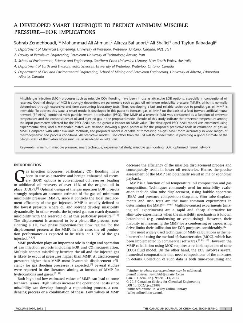
A specific volume of reservoir fluid was charged to a glass beadpacked column with a height of 1.8 m. Then, the porous mediumwas stabilised at the reservoir temperature of 205◦F and initial testpressure of 5985 psig. The injection gas was also stabilised at theabove desired temperature and pressure. Injection was continuedgradually into the tube to displace the oil. The initial gas flow ratewas ∼6 cm3/h. This flow rate was kept for 5 h to launch a stableoil–gas interface. The injected gas flow rate was then increased to8 cm3/h and continued until approximately 1.4 pore volumes ofgas or having a gas–oil ratio above 100 000 scf/bbl. The weightsof oil displaced and the volume of the flashed gas coming outfrom the tube were measured at regular intervals. At the end ofeach displacement run, the packed physical system was depres-surised by allowing the gas to release through a trap. This helpscollecting any of the oil remaining in the column. Thereafter, thecollected oil was weighed. The line and fittings at both ends ofthe column were also cleaned with a solvent and the oil recov-ered from this process was weighed and recorded as the residualoil. The glass bead packed column was weighed before and afterthe displacement to ensure if any oil was left in the column. Theweight difference was then added to obtain total residual oil. Thisprocedure was repeated at the reservoir temperature and but dif-
Figure 1. A picture of slim tube apparatus.
ferent pressures such as 3985, 4985, 5185 and 5485 psig. Figure 1shows a schematic of the slim tube apparatus.
In addition to the data generated from experimental part of thisstudy, data from the literature were also used in developing thePSO–ANN model. The data used for developing the neural-geneticmodel are from Alston et al.,[8] Cardenas,[40] Dong,[41] Donget al.,[42] Eissa and Shokir,[16] Emera and Sarma,[34,35] Frimodiget al.,[36] Gardner et al.,[37] Gharbi and Elsharkawy,[43] Graue andZana,[38] Jacobson,[44] Metcalfe,[11] Okuno,[33] Sebastian et al.[24]
and Yuan et al.[45] These data are presented in Appendix B.
ARTIFICIAL NEURAL NETWORK
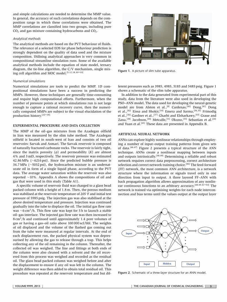
ANNs can explore highly nonlinear relationships through employ-ing a number of input–output training patterns from given setsof data.[46,47] Figure 2 presents a typical structure of the ANNtechnique. ANNs create a nonlinear mapping between inputsand outputs intrinsically.[48,49] Determining a reliable and robustnetwork requires correct data preprocessing, correct architectureselection and correct network training choice.[50] The feed-forward(FF) network, the most common ANN architecture, is a networkstructure where the information or signals travel only in onedirection from input to output. A three layered FF–ANN withback propagation algorithm allows approximation of any nonlin-ear continuous functions to an arbitrary accuracy.[48,49,51–53] Thenetwork is trained via optimising weights for each node intercon-nection and bias terms until the values output at the output layer
Figure 2. Schematic of a three-layer structure for an ANN model.
| VOLUME 9999, 2013 | | THE CANADIAN JOURNAL OF CHEMICAL ENGINEERING | 3 |

neurons are very close enough to the actual outputs. The meansquared error of the network (MSEnet) is defined as:
MSEnet = 12
G∑k=1
m∑j=1
[Yj(k) − Tj(k)
]2 (1)
where m is the number of output nodes, G is the number of train-ing samples, Yj(k) is the expected output and Tj(k) is the actualoutput. When the MSEnet approaches to zero, the error of networklowers.
During the construction of the intelligent technique, the dataare divided into two sets: training and validating or testing datasets. In training a network, the objective is finding an optimumset of weights. When the number of weights is higher than thenumber of available data, the error in fitting the nontrained datainitially decreases then increases as the network becomes over-trained. In contrast, when the number of weights is smaller thanthe number of data, the over-fitting problem is not crucial.
In this study, an ANN was utilised to predict the value ofgas–oil MMP. The ANN model with back propagation networkwas trained by the Levenberg–Marquardt approach for predictionof MMP. The most proper ANN architecture for the current studywas 9-4-10-1 (9 input units, 4 neurons in first hidden layer, 10neurons in second hidden layer, 1 output neuron). The trans-fer functions in hidden and output layer are sigmoid and linear,respectively.
PARTICLE SWARM OPTIMISATION
Kennedy and Eberhart introduced PSO to solve problems incontinuous search space. PSO was found on an image forsocial interaction and communication (e.g. bird flocking and fishtraining).[54–56] The PSO technique applies social laws to searchin the design space by organising the trajectories of a series ofindependent particles. The location of each particle (Xi), whichindicates a specific solution to the problem, is utilised to calcu-late the optimised extent of the fitness function. Each particlehas different positions during the optimisation process. The par-ticle position is changed to explore the solution in space whichvaries its corresponding velocity continuously. The key PSO oper-ator is the velocity update, which considers the best position. Thebest position is presented in terms of the fitness value for all theparticles during their paths (Pt
g) and also the best position thatthe agent itself has reached during its search (Pt
i ). This processleads to migration of the entire swarm particles toward the globaloptimum.[54,57]
In the PSO, every particle travels around at each iteration, basedon its velocity and location. The cost function for each particleis evaluated for ranking its current position. Normally, the par-ticles velocities build up too fast and converge to a suboptimalsolution.[54] Shi and Eberhart[57] introduced the concept of inertiaweight (ω) to the original version of PSO in order to reduce thevelocity. Then, the velocity of the particle is updated stochasticallyaccording to the following relationship:
Vt+1i = ωVt
i + c1rt1(P
ti − Xt
i ) + c2rt2(P
tg − Xt
i ) (2)
Xt+1i = Xt
i + Vt+1i (3)
where Vti is defined as the velocity vector at iteration t, r1 and r2
are random numbers in the range [0, 1], Ptg represents the best ever
particle position of particle i and Pti refers to the global best posi-
tion in the swarm until iteration t.[54,57] Other parameters in theabove equations are problem dependent variables. For instance, c1
and c2 denote ‘trust’ parameters indicating how much confidencethe current particle c1 (cognitive parameter) has in itself and howmuch confidence c2 (social parameter) has in the swarm, and ω
represents the inertia weight. The second term in Equation (2)has an important role in the PSO convergence behaviour since itis used to control the exploration abilities of the swarm. It has alsodirect effect on the current velocity, which is based on the historyof velocities. High inertia weights make possible a wide velocityupdates that lead to a global exploration of the search space. Smallinertia values assist the velocity updates get the regions near thedesign space. It should be noted here that Equation (2) indicateshow the particle velocity is continuously updated, and updating ofthe positions for the ‘flying’ particles is conducted using Equation(3).
Typically, the inertia weight (ω) decreases linearly with theiteration number as follows:
ωt = ωmax −(
ωmax − ωmin
tmax
)t (4)
where ωmin and ωmax are the initial and final values of the inertiaweight, respectively, tmax is the current iteration number and ωmax
is the maximum number of iterations used in PSO. The values ofωmax = 0.9 and ωmin = 0.4 are the proper value through empiricalstudies.[54,57]
The following steps were taken after computing the requiredparameters for network training: (a) normalising the inputs andoutput; (b) creating the network; (c) dividing up samples for test-ing and training; (d) training the network; (e) simulating thenetwork; and (f) plotting the regression.
To create a proper neural network, a Roulette Wheel Parent(RWP) selection was performed to select two parents (chro-mosomes) from the population for generation of two children(new chromosomes) using the reproduction operators.[54,57] Thismethodology is employed because it is quicker than other tech-niques such as tournament parent selection. A one-point crossoverwith a probability (P(c)) of 100% is used. After crossover and pro-duction of two children chromosomes, one gene is selected fromeach child chromosome to change its value (mutation probabil-ity (P(m)) = 1%) by adding a random value to its old value asfollows:
New value = ˇ × Old value + � × Random value 0 ≤ ˇ ≤ 1 &
0 ≤ � ≤ 1 (5)
where ˇ = 1.45 and � = 0.40 are selected in this study. These val-ues are based on ANN performance, where ˇ is increased and � isdecreased to detect any improvement in the fitness value; other-wise, the process is reversed. In addition, this technique facilitatesthe use of a part of the last reached solution. The optimisation isdone with the PSO. The final network is then trained by BP upto the acceptable extent of mean squared error (MSE), and thenetwork performance is verified through introducing the hiddentesting patterns.
The performance of the PSO–ANN model developed inthis study was evaluated using various standard statisticalcriteria. The statistical parameters are correlation coefficient(R2), MSE, mean absolute percentage error (MAPE) andmaximum absolute percentage error (MAAE). Appendix C
| 4 | THE CANADIAN JOURNAL OF CHEMICAL ENGINEERING | | VOLUME 9999, 2013 |

Table 1. Different network structures to select the best for PSO–ANN network
Objective Number of neurons in Number of neurons in Training MomentumRun function value the first hidden layer the second hidden layer coefficient coefficient
1 0.312 5 8 0.733 0.6712 0.328 4 10 0.746 0.7133 0.334 5 9 0.739 0.6824 0.341 4 10 0.738 0.6915 0.348 3 8 0.751 0.7256 0.305 6 7 0.741 0.699Average: 0.328
presents the corresponding formulas for the above statisticalparameters.
RESULTS AND DISCUSSION
An erroneous MMP prediction leads to major issues in EORschemes. For instance, recommendation for a too high operat-ing level of MMP leads to additional operational costs and safetyissues. If MMP is underestimated, then the miscible displacementprocess becomes unsuccessful and results in system deficiency aswell. Hence, higher accuracy in prediction of the MMP predictionis rewarding.
Parameters considered for the proposed ANN model were reser-voir temperature, molecular weight (Mw) of C+
5 , gas composition,H2S composition, C1, C2–C4, C+
5 and N2 compositions as input.Then, the PSO is used as neural network optimisation algorithm,and the MSE was implemented as a cost function. The goal inthe proposed algorithm was to minimise the cost function. Everyweight in the network was initially set in the range of [−1, 1],and every initial particle was a set of weights generated randomlyin the range of [−1, 1].
The MMP data were divided into two data sets consisting oftraining and validation test data. Two hundred and five data sam-ples were chosen by a random number generator for networktraining. The remaining 100 samples were put aside to be used fortesting the network’s integrity and robustness. In order to obtainthe performance information, a total of six runs were carried out.The examined information is shown in Table 1. As the average ofthe objective function value is close to the value calculated fromrun 2, the characteristics of the network structure are selectedaccording to run 2. Therefore, this will be the network that couldconstruct the optimum structure for MMP prediction. The opti-mum structure depends on the data used and composition of themixture. Hence, it is expected to have different optimum struc-
tures for different sets of data. It can be concluded that the trainingdata set dictates the type of the network structure. As shown inTable 1, the best ANN architecture for the case studied here is9-4-10-1 (9 input units, 4 neurons in first hidden layer, 10 neuronsin second hidden layer, 1 output neuron).
In order to examine the suitability of the PSO–ANN networkselected here, different numbers of neurons for the first and sec-ond hidden layers were tried. The impact of number of hiddenneurons on the effectiveness of PSO–ANN system is given inTable 2, based on a statistical analysis. The performance of thedeveloped neural network was improved as the number of hid-den neurons increased from 7 to 10. However, further increase inthe number of hidden neurons in the second layer lowered theperformance of the PSO–ANN system. According to the values ofR2, MSE, MAPE and MAAE, the optimum configuration for thePSO–ANN model within the ranges of input variables included 4and 10 neurons in the first hidden layer and second hidden layer,respectively (see Table 2), since the highest R2 and the lowest val-ues for various error functions defined here were attained for thisnetwork structure. Higher numbers of neurons (11 for the secondhidden layer) were not chosen in order to avoid over-training ofthe PSO–ANN model. The results obtained from this statisticalstudy confirm that the optimum configuration for PSO–ANN wasselected appropriately.
The number of particles in the PSO–ANN dictates the quantity ofthe space covered in the problem. Table 3 shows the effect of num-ber of particles on the performance of the developed intelligentmodel. As seen in Table 3, the PSO–ANN performance increaseswith increase in the number of particles from 15 to 21. The devel-oped neural network model is not able to describe well the databehaviour at numbers of particles equal to 15 and 18 becausethe space covered in the problem is not adequate for these num-bers. Then, a decrease in the PSO–ANN performance was observedbased on the values of R2 and error percentage when the number
Table 2. Effect of number of hidden neurons on performance of the PSO–ANN in training phase
Number of neurons in Number of neurons infirst hidden layer second hidden layer R2 MSE MAPE MAAE
4 9 0.9452 0.0658 7.5496 11.43524 10 0.9738 0.0717 5.5681 8.31764 11 0.9169 0.0626 6.0045 9.22955 9 0.9376 0.0754 5.6632 8.29995 10 0.9641 0.0736 5.5877 8.01075 11 0.9434 0.0768 5.9718 8.99716 9 0.9014 0.0941 7.3671 9.00456 10 0.8978 0.0975 8.4232 9.50246 11 0.9107 0.0854 5.6709 9.8877
| VOLUME 9999, 2013 | | THE CANADIAN JOURNAL OF CHEMICAL ENGINEERING | 5 |

Table 3. Effect of number of particles on performance of the PSO–ANN
Training Testing
Number of particles R2 MSE MAPE MAAE R2 MSE MAPE MAAE
15 0.9695 0.0565 5.4468 9.7943 0.9275 0.0658 6.5496 10.875218 0.9384 0.0713 7.1563 11.8652 0.8944 0.0717 8.1865 12.257620 0.9742 0.0559 6.5422 9.3095 0.9559 0.0626 7.2054 10.110821 0.9923 0.0354 2.9977 7.0057 0.9774 0.0587 3.1866 7.997922 0.9716 0.0974 4.8863 10.9651 0.9457 0.0755 5.7782 11.411625 0.9722 0.0957 4.7791 10.4587 0.9468 0.0749 5.5671 11.0505
of particles was set on 22 (see Table 3). The main reason behindthis decline is that the space covered in the problem appears tobe too wide. The model efficiency was improved slightly whenthe number increased to 25. Hence, it can be concluded that theoptimum number of particles is 21. It should be also noted herethat as the number of particles increases, the greater amount ofspace is covered in the problem, leading to a slower optimisationprocess.
The gas–oil MMP predictions in the training and test phases areshown in Figures 3 and 4 for the ANN method and Figures 5 and6 for the PSO–ANN model. In this study, the developed PSO–ANNmodel was compared to the ANN model and four common cor-
a
b
Figure 3. Measured versus predicted gas–oil MMP from the ANN model:(a) training phase and (b) testing phase.
relations (Alston et al.,[8] Emera and Sarma,[34,35] Riedel[19] andYuan et al.[45]) to examine the effectiveness of the PSO–ANN. Theselected MMP equations were considered as powerful empiricalcorrelations to predict the MMP with high accuracy. Figures 4,6–10 show the extent of the match between the measured and pre-dicted gas–oil MMP values using the ANN, PSO–ANN, Alston etal.,[8] Emera and Sarma,[34,35] Yuan et al.[45] and Riedel[19] modelsas scatter diagrams, respectively.
The input variables of an ANN system are frequently of varioustypes with different orders of magnitudes, such as temperature(T) and molecular weight (Mw) in the case studied here. Thesame thing usually occurs for the output parameters. Thus, it isnecessary to normalise the input and output parameters based onranges of data as they fall within a particular range, for instance,
a
b
Figure 4. Performance of the ANN model based on R2: (a) training and(b) testing.
| 6 | THE CANADIAN JOURNAL OF CHEMICAL ENGINEERING | | VOLUME 9999, 2013 |

a
b
Figure 5. Measured versus predicted MMP using the PSO–ANN model:(a) training and (b) testing.
setting minimum −1 and the maximum +1 to have all the datawithin the interval [−1, 1]. The legend of the vertical axis inFigures 3–6 presents normalised MMP calculated using the fol-lowing expression:
Normalised MMP = 2(MMP − MMPmin)(MMPmax − MMPmin)
− 1 (6)
where MMPmin and MMPmax are the minimum and maximumMMP of the data used in this study, respectively.
As can be seen in Figures 3–6, a comparison between pre-dicted and measured MMP values (obtained from slim tube test)for the Azadegan oilfield in Iran at training and testing phasesfor both hybrid PSO–ANN and conventional ANN models wasconducted in this study. As shown in Figures 3–6, the outputsof the models simulated with PSO–ANN and ANN exhibit anacceptable agreement with the actual data of the target field andalso the experimental data available in the literature. However,the PSO–ANN model exhibits a higher precision in prediction ofMMP compared with ANN as, for instance, MSE and MAAE forPSO–ANN are 0.0269 and 6.43 in contrast to 0.4567 and 12.66for ANN, respectively (Table 4). The values of R2 and MAPE forthese two models confirm the above statement, indicating higher
a
b
Figure 6. Performance of the developed PSO–ANN model based on R2:(a) training phase and (b) testing phase.
effectiveness of the PSO–ANN. The fairly significant differencesin the magnitudes of relative errors for the PSO–ANN and ANNclearly show the impact of adding PSO to conventional ANN inestimation of important variables (e.g. MMP, bubble pressure andpermeability) involved in petroleum engineering, where settingan appropriate production management and selecting a properEOR scheme highly depend on the accuracy of the process andthermodynamic variables while performing the required analyt-ical and numerical computations prior to implementation of atechnically and economically feasible process.
Figure 7. Performance of the Alston et al.[8] correlation in predictingMMP based on R2.
| VOLUME 9999, 2013 | | THE CANADIAN JOURNAL OF CHEMICAL ENGINEERING | 7 |

Figure 8. Performance of the Emera and Sarma[34,35] correlation inpredicting MMP based on R2.
Figure 9. Performance of the Yuan et al.[45] model in predicting MMPbased on R2.
Table 4 gives the R2, MSE, MAPE and MAAE values for the dif-ferent models of the validation phases. It can be observed that theperformance of PSO–ANN model is better than other models. Theproposed PSO–ANN model produces lower error levels comparedwith the other models tested. In addition, the developed model haslower calibration errors than the models suggested by researcherssuch as Alston et al.[8] and Emera and Sarma.[34,35] For example,
Figure 10. Performance of the Riedel[19] model in predicting MMPbased on R2.
the neural-genetic model developed here is able to enhance theperformance of the Alston et al.[8] model in MMP prediction overthe training phase by lowering MSE and MAPE values to ∼96%and ∼66%, respectively. Also, the higher value of R2 for PSO–ANNcompared with the other MMP forecast models observed in thisstudy indicates a very satisfactory performance for the developedmodel.
The proposed PSO–ANN model enhanced the results from themodel developed by Yuan et al.,[45] and the MSE and MAPE werereduced to ∼97.2% and ∼72.1%, respectively. Improvements inestimation of MMP with respect to correlation coefficient (R2) dur-ing the validation phase were approximately 15% and 17% forthe models proposed by Alston et al.[8] and Yuan et al.,[45] corre-spondingly. It is also important to note that MSE and MAPE wereimproved by the proposed PSO–ANN model about 97% and 82%for the Emera and Sarma model[34,35] and 96.9% and 71.2% forRiedel,[19] respectively, indicating that the PSO–ANN model pro-posed is a proper tool for fast, inexpensive and reliable estimationof the MMP.
As shown in Table 4, the models proposed by Yuan et al.,[45]
Riedel,[19] Emera and Sarma[34,35] and Alston et al.[8] are notconsidered as good predictive correlations for MMP within thethermodynamic conditions of the fluid samples used in this study.The values of R2 and MAAE in Table 4 for various techniques con-vey the message that the PSO–ANN enhances the accuracy of MMPpredictions considerably as the value of MAAE is much lower forthe PSO–ANN compared to that for the other methods describedin this research. It can be concluded here that all prediction mod-els other than the developed PSO–ANN model fail to determinean accurate value for MMP of the hydrocarbon mixtures existingin the Azadegan oilfield, Iran.
Table 4. Performance of the proposed PSO–ANN versus ANN and common empirical models
Parameter PSO–ANN model ANN model Yuan et al.[45] Emera and Sarma[34,35] Alston et al.[8] Riedel[19]
R2 0.9903 0.8997 0.8456 0.7367 0.8613 0.8404MSE 0.0269 0.4567 0.9567 0.9874 0.7235 0.8753MAPE 2.52 5.95 9.11 13.98 7.36 8.75MAAE 6.43 12.66 75.86 110.27 95.01 80.62
| 8 | THE CANADIAN JOURNAL OF CHEMICAL ENGINEERING | | VOLUME 9999, 2013 |
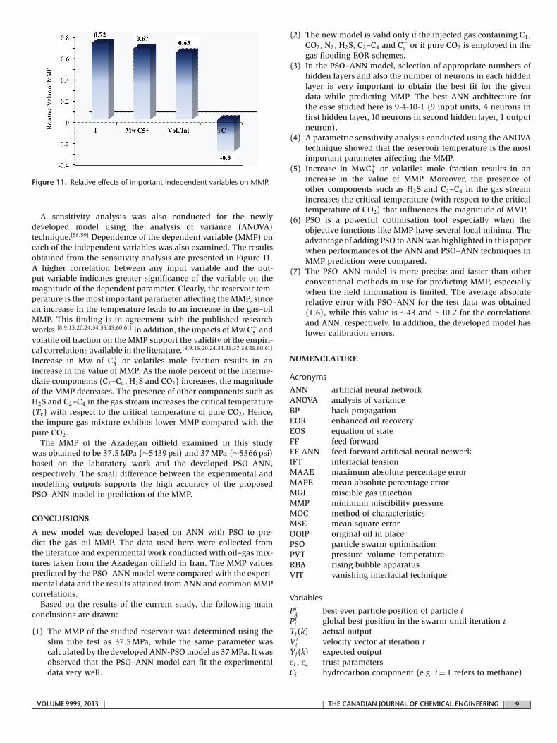
Figure 11. Relative effects of important independent variables on MMP.
A sensitivity analysis was also conducted for the newlydeveloped model using the analysis of variance (ANOVA)technique.[58,59] Dependence of the dependent variable (MMP) oneach of the independent variables was also examined. The resultsobtained from the sensitivity analysis are presented in Figure 11.A higher correlation between any input variable and the out-put variable indicates greater significance of the variable on themagnitude of the dependent parameter. Clearly, the reservoir tem-perature is the most important parameter affecting the MMP, sincean increase in the temperature leads to an increase in the gas–oilMMP. This finding is in agreement with the published researchworks.[8,9,15,20,24,34,35,45,60,61] In addition, the impacts of Mw C+
5 andvolatile oil fraction on the MMP support the validity of the empiri-cal correlations available in the literature.[8,9,15,20,24,34,35,37,38,45,60,61]
Increase in Mw of C+5 or volatiles mole fraction results in an
increase in the value of MMP. As the mole percent of the interme-diate components (C2–C4, H2S and CO2) increases, the magnitudeof the MMP decreases. The presence of other components such asH2S and C2–C4 in the gas stream increases the critical temperature(Tc) with respect to the critical temperature of pure CO2. Hence,the impure gas mixture exhibits lower MMP compared with thepure CO2.
The MMP of the Azadegan oilfield examined in this studywas obtained to be 37.5 MPa (∼5439 psi) and 37 MPa (∼5366 psi)based on the laboratory work and the developed PSO–ANN,respectively. The small difference between the experimental andmodelling outputs supports the high accuracy of the proposedPSO–ANN model in prediction of the MMP.
CONCLUSIONS
A new model was developed based on ANN with PSO to pre-dict the gas–oil MMP. The data used here were collected fromthe literature and experimental work conducted with oil–gas mix-tures taken from the Azadegan oilfield in Iran. The MMP valuespredicted by the PSO–ANN model were compared with the experi-mental data and the results attained from ANN and common MMPcorrelations.
Based on the results of the current study, the following mainconclusions are drawn:
(1) The MMP of the studied reservoir was determined using theslim tube test as 37.5 MPa, while the same parameter wascalculated by the developed ANN-PSO model as 37 MPa. It wasobserved that the PSO–ANN model can fit the experimentaldata very well.
(2) The new model is valid only if the injected gas containing C1,CO2, N2, H2S, C2–C4 and C+
5 or if pure CO2 is employed in thegas flooding EOR schemes.
(3) In the PSO–ANN model, selection of appropriate numbers ofhidden layers and also the number of neurons in each hiddenlayer is very important to obtain the best fit for the givendata while predicting MMP. The best ANN architecture forthe case studied here is 9-4-10-1 (9 input units, 4 neurons infirst hidden layer, 10 neurons in second hidden layer, 1 outputneuron).
(4) A parametric sensitivity analysis conducted using the ANOVAtechnique showed that the reservoir temperature is the mostimportant parameter affecting the MMP.
(5) Increase in MwC+5 or volatiles mole fraction results in an
increase in the value of MMP. Moreover, the presence ofother components such as H2S and C2–C4 in the gas streamincreases the critical temperature (with respect to the criticaltemperature of CO2) that influences the magnitude of MMP.
(6) PSO is a powerful optimisation tool especially when theobjective functions like MMP have several local minima. Theadvantage of adding PSO to ANN was highlighted in this paperwhen performances of the ANN and PSO–ANN techniques inMMP prediction were compared.
(7) The PSO–ANN model is more precise and faster than otherconventional methods in use for predicting MMP, especiallywhen the field information is limited. The average absoluterelative error with PSO–ANN for the test data was obtained(1.6), while this value is ∼43 and ∼10.7 for the correlationsand ANN, respectively. In addition, the developed model haslower calibration errors.
NOMENCLATURE
Acronyms
ANN artificial neural networkANOVA analysis of varianceBP back propagationEOR enhanced oil recoveryEOS equation of stateFF feed-forwardFF-ANN feed-forward artificial neural networkIFT interfacial tensionMAAE maximum absolute percentage errorMAPE mean absolute percentage errorMGI miscible gas injectionMMP minimum miscibility pressureMOC method-of characteristicsMSE mean square errorOOIP original oil in placePSO particle swarm optimisationPVT pressure–volume–temperatureRBA rising bubble apparatusVIT vanishing interfacial technique
Variables
Ptg best ever particle position of particle i
Pti global best position in the swarm until iteration t
Tj(k) actual outputVt
i velocity vector at iteration tYj(k) expected outputc1, c2 trust parametersCi hydrocarbon component (e.g. i = 1 refers to methane)
| VOLUME 9999, 2013 | | THE CANADIAN JOURNAL OF CHEMICAL ENGINEERING | 9 |

G number of training samplesInt intermediate componentsK permeability (mD)m number of output nodesMw molecular weightr1, r2 random numberR2 coefficient of determinationT reservoir temperatureTc critical temperaturevol volatile components
Greek Symbols
ω inertia weight� porosityˇ a constant coefficient in Equation (5)� a constant coefficient in Equation (5)
Subscripts
i particle imax maximummin minimum
Superscripts
M measuredNet networkP predictedt iteration number
Appendix A
Table A1 shows the compositions of oil and gas phases of the realcase employed in this study.
Appendix B
The main part of the experimental data used in this study todevelop the PSO–ANN model is presented in Table B1. To constructthe training network, a large volume of the MMP data availablein the literature were employed to have a more robust and preciseneural network model.
Appendix C
R2, MSE, MAPE and MAAE are the statistical parameters to test theaccuracy of the PSO–ANN model compared with common corre-lations. The equations to compute the above parameters and alsothe corresponding description are as follows:
R2 is a statistic parameter which gives information on good-ness of fit in a model. In regression analysis or fitting of a model,the R2 coefficient is a statistical measure of how well the modelline approximates the real data points. An R2 of 1.0 indicates themodel line perfectly fits the data. The following equation showsthe mathematical definition of R2[58,59]:
R2 =
n∑i=1
(MMPPi − MMPM)2
n∑i=1
(MMPMi − MMPM)2
(C.1)
where MMPM and MMPP are the measured MMP and predictedMMP, respectively. MMPM represents the average of the measuredMMP data.
Table A1. Compositions of the oil and gas used in the MMPexperimental tests
Pure gas Gas mixture ReservoirComponent (mol%) (mol%) fluid (mol%)
H2 0.00 0.00 0.00H2S 0.00 0.00 0.00CO2 100.00 5.00 2.12N2 0.00 0.52 0.19C1 0.00 40.56 17.34C2 0.00 18.59 8.15C3 0.00 15.12 6.62iC4 0.00 2.77 1.30nC4 0.00 8.35 4.26C5 0.00 0.00 0.00iC5 0.00 4.18 2.19nC5 0.00 4.38 2.60C6 0.00 0.53 1.77C7 0.00 0.00 1.85C8 0.00 0.00 3.00C9 0.00 0.00 2.23C10 0.00 0.00 2.87C11 0.00 0.00 3.36C12 0.00 0.00 3.39C13 0.00 0.00 3.29C14 0.00 0.00 2.89C15 0.00 0.00 2.76C16 0.00 0.00 2.48C17 0.00 0.00 2.11C18 0.00 0.00 1.95C19 0.00 0.00 1.92C20 0.00 0.00 1.65C+
20 0.00 0.00 17.71
The mean squared error (MSE) is a measure of how close afitted line or developed model is to data points. The smaller theMSE, the closer the fit (or model) is to the actual data. The MSEhas the units squared of whatever is plotted on the vertical axis.MSE is described by the following relationship[58,59]:
MSE =
n∑i=1
(MMPMi − MMPP
i )2
n(C.2)
where n is the number of samples.Mean absolute percentage error (MAPE) is the measure of accu-
racy in a fitted time series value in statistics (%) and is definedas[58,59]:
MAPE = 1n
n∑i=1
∣∣∣∣MMPMi − MMPP
i
MMPMi
∣∣∣∣ × 100 (C.3)
The other performance measure that was employed in this studyto evaluate the usefulness of the training and testing phases ismaximum absolute percentage error (MAAE) as follows[58,59]:
MAAE% = max∣∣MMPP
i − MMPMi
∣∣MMPM
i
× 100 (C.4)
| 10 | THE CANADIAN JOURNAL OF CHEMICAL ENGINEERING | | VOLUME 9999, 2013 |

Table B1. Experimental data for gas–oil MMP from various studies
Composition of gas stream Oil propertiesExperimental
Run no. CO2 (%) C1 (%) N2 (%) C2–C4 (%) H2S (%) T (◦C) MwC+5 Vol./Int. MMP (MPa) Research
1 100 0 0 0 0 54.44 185.83 0.6 10.34 Alston et al.[8]
2 100 0 0 0 0 61.11 185.83 0.14 10.34 Alston et al.[8]
3 100 0 0 0 0 57.78 202.61 0.42 11.71 Alston et al.[8]
4 90.5 0 0 9.5 0 71.11 221 5.9 18.61 Gharbi and Elsharkawy[43]
5 100 0 0 0 0 54.44 185.83 0.14 9.48 Gharbi and Elsharkawy[43]
6 100 0 0 0 0 71.11 221 5.9 23.43 Gharbi and Elsharkawy[43]
7 100 0 0 0 0 37.78 235.56 2.58 16.54 Gharbi and Elsharkawy[43]
8 100 0 0 0 0 112.22 213.5 1.16 24.13 Gharbi and Elsharkawy[43]
9 100 0 0 0 0 54.44 185.83 0.67 10.34 Gharbi and Elsharkawy[43]
10 92.5 7.5 0 0 0 54.44 185.83 0.14 10.34 Gharbi and Elsharkawy[43]
11 100 0 0 0 0 110 180.6 0.91 20.19 Gharbi and Elsharkawy[43]
12 90 10 0 0 0 54.44 185.83 0.73 13.09 Gharbi and Elsharkawy[43]
13 95 0 0 5 0 71.11 221 5.9 18.61 Gharbi and Elsharkawy[43]
14 86.4 10.7 0 2.9 0 73.33 227 7.71 23.09 Gharbi and Elsharkawy[43]
15 87.5 0 6.3 6.2 0 76.11 227 7.71 23.15 Gardner et al.[37]
16 79.2 0 8.8 12 0 76.11 227 7.71 23.15 Gardner et al.[37]
17 100 0 0 0 0 67.78 203.81 1.35 16.88 Gardner et al.[37]
18 100 0 0 0 0 42.78 196.1 0.82 10.61 Frimodig et al.[36]
19 90 10 0 0 0 54.44 171.2 0.93 12.4 Cardenas[40]
20 100 0 0 0 0 54.44 171.2 0.93 10.98 Cardenas[40]
21 80 0 0 20 0 65.56 187.27 1.51 10.49 Metcalfe[11]
22 45 10 0 0 45 40.56 187.8 0.74 8.82 Metcalfe[11]
23 50 0 0 0 50 57.22 187.8 0.74 8.96 Dong et al.[42]
24 90 0 0 10 0 65.56 187.27 1.51 11.03 Dong et al.[42]
25 100 0 0 0 0 40.56 187.8 0.74 8.27 Jacobson[44]
26 80 0 0 20 0 65.56 187.27 1.51 12.87 Jacobson[44]
27 60 20 0 0 20 57.22 187.8 0.74 17.23 Shokir and Eissa[16]
28 100 0 0 0 0 65.56 187.27 1.51 13.44 Shokir and Eissa[16]
29 90 10 0 0 0 40.56 187.8 0.74 11.07 Shokir and Eissa[16]
30 80 20 0 0 0 40.56 187.8 0.74 14.86 Shokir and Eissa[16]
31 100 0 0 0 0 48.89 187.27 1.51 11.03 Shokir and Eissa[16]
32 80 0 0 20 0 48.89 187.27 1.51 9.65 Shokir and Eissa[16]
33 50 0 0 0 50 40.56 187.8 0.74 6.53 Shokir and Eissa[16]
34 80 0 0 20 0 48.89 187.27 1.51 7.92 Shokir and Eissa[16]
35 80 20 0 0 0 57.22 187.8 0.74 18.61 Shokir and Eissa[16]
36 67.5 10 0 0 22.5 57.22 187.8 0.74 12.4 Shokir and Eissa[16]
37 60 20 0 0 20 40.56 187.8 0.74 14.06 Shokir and Eissa[16]
38 90 0 0 10 0 48.89 187.27 1.51 7.89 Shokir and Eissa[16]
39 90 10 0 0 0 57.22 187.8 0.74 15.33 Shokir and Eissa[16]
40 90 0 0 10 0 65.56 187.27 1.51 8.96 Shokir and Eissa[16]
41 40 20 0 0 40 57.22 187.8 0.74 12.4 Shokir and Eissa[16]
42 45 10 0 0 45 57.22 187.8 0.74 10.37 Shokir and Eissa[16]
43 90 0 0 10 0 48.89 187.27 1.51 9.3 Shokir and Eissa[16]
44 67.5 10 0 0 22.5 40.56 187.8 0.74 10.25 Shokir and Eissa[16]
45 100 0 0 0 0 57.22 187.8 0.74 11.71 Shokir and Eissa[16]
46 100 0 0 0 0 32.22 187.8 0.74 6.89 Shokir and Eissa[16]
47 75 0 0 0 75 57.22 187.8 0.74 10.3 Shokir and Eissa[16]
48 90 0 0 10 0 65.56 187.27 1.51 13.02 Shokir and Eissa[16]
49 90 0 0 10 0 48.89 187.27 1.51 9.99 Shokir and Eissa[16]
50 40 20 0 0 40 40.56 187.8 0.74 12.09 Emera and Sarma[34,35]
51 75 0 0 0 25 40.56 187.8 0.74 7.53 Emera and Sarma[34,35]
52 92.25 0 0 7.75 0 112.22 213.5 1.16 19.67 Emera and Sarma[34,35]
53 100 0 0 0 0 71.11 207.9 0.32 15.51 Yuan et al.[45]
54 95 4.9 0.1 0 0 71.11 207.9 0.32 16.81 Yuan et al.[45]
55 100 0 0 0 0 42.78 204.1 0.82 10.34 Sebastian et al.[24]
Vol., volatile oil fraction; Int., intermediate oil fraction.
| VOLUME 9999, 2013 | | THE CANADIAN JOURNAL OF CHEMICAL ENGINEERING | 11 |

REFERENCES
[1] R. B. Grigg, D. S. Schechter, ‘‘State of the Industry in CO2
Floods’’ in SPE Annual Technical Conference andExhibition, SPE Paper 38849, San Antonio, Texas, USA 5–8October 1997.
[2] E. H. Benmekki, G. A. Mansoori, ‘‘Accurate VaporizingGas-Drive Minimum Miscibility Pressure Prediction’’, inEastern Regional Meeting of SPE, SPE paper 15677,Richardson, Texas, USA 1986.
[3] J. N. Jaubert, L. Wolff, L. Avaullee, E. Neau, Ind. Eng.Chem. Res. 1998, 37, 4854.
[4] G. A. Mansoori, T. S. Jiang, S. Kawanaka, Arabian J. Sci.Eng. 1988, 13, 120.
[5] F. Stalkup, SPE Monograph, Chapter 8, SPE publication,Dallas,Texas 1983, pp. 137–158.
[6] Y. Wang, F. M. Orr, J. Pet. Sci. Eng. 2000, 27, 151.[7] W. F. Yellig, R. S. Metcalfe, J. Pet. Technol. 1980, 32, 160.[8] R. B. Alston, G. P. Kokolis, C. F. James, SPE J. 1985, 25,
268.[9] L. W. Holm, V. A. Josendal, J. Pet. Technol. 1974, 26, 1427.
[10] J. P. Johnson, J. S. Pollin, ‘‘Measurement and Correlation ofCO2 Miscibility Pressures’’, in SPE/DOE Enhanced OilRecovery Symposium, Tulsa, Oklahoma, USA 5–8 April 1981.
[11] R. S. Metcalfe, SPE J. 1982, 22, 219.[12] K. Ahmadi, R. Johns, ‘‘Multiple Mixing-Cell Method for
MMP Calculations’’, in SPE Annual Technical Conferenceand Exhibition, Denver, Colorado, USA, 21–24 September2008.
[13] A. M. Elsharkawy, Energy Fuels 1996, 10, 443.[14] J. N. Jaubert, L. Avaullee, C. Christophe Pierre, Ind. Eng.
Chem. Res. 2002, 41, 303.[15] D. N. Rao, J. I. Lee, J. Pet. Sci. Eng. 2002, 35, 247.[16] M. Eissa, E. M. Shokir, J. Pet. Sci. Eng. 2007, 58, 173.[17] R. M. Enrick, R. M. Holder, B. I. Morsi, SPE Res. Eng. 1988,
3, 81.[18] F. M. Orr, M. K. Silva, ‘‘Effect of Oil Composition on
Minimum Miscibility Pressures, Part 2: Correlation’’, in SPEAnnual Technical Conference and Exhibition, Paper SPE14150, Las Vegas, USA, 22–25 September 1985.
[19] K. L. Riedel, A Correlation for Carbon Dioxide MinimumMiscibility Pressure, M.Sc. Thesis, Colorado School ofMines, USA, 1985.
[20] A. L. Benham, W. E. Dowden, W. J. Kunzman, Trans. AIME1959, 216, 388.
[21] C. Cronquist, ‘‘Carbon Dioxide Dynamic Miscibility withLight Reservoir Oils’’, in Proceedings of the Fourth AnnualUS DOE Symposium, Tulsa, OH, USA 1978.
[22] F. S. Kovarik, ‘‘A Minimum Miscibility Pressure StudyUsing Impure CO2 and West Texas Oil Systems: Data Base,Correlations and Compositional Simulation’’, in SPEProduction Technology Symposium, Paper SPE 14689,Lubbock, 11–12 November 1985.
[23] N. Mungan, J. Can. Pet. Technol. 1981, 20, 28.[24] H. M. Sebastian, R. S. Wenger, T. A. Renner, JPT 1985, 37,
268.[25] G. Zhao, H. Adidharma, B. Towler, M. Radosz, ‘‘Minimum
Miscibility Pressure Prediction Using Statistical AssociatingFluid Theory: Two and Three-Phase Systems’’, in SPE
Annual Technical Conference and Exhibition, San Antonio,Texas, USA, 24–27 September 2006.
[26] H. F. Huang, G. H. Huang, G. M. Dong, G. M. Feng, J. Pet.Sci. Eng. 2003, 37, 83.
[27] B. C. Ridha, R. B. Gharbi, A. M. Elsharkawy, SPE Res. Eva.Eng. 1999, 2, 255.
[28] J. Sjoberg, L. Ljung, ‘‘Overfitting, Regularization, andSearching for Minimum in Neural Networks’’, in FourthIFAC International Symposium on Adaptive Systems inControl Signal and Processing, Grenoble, France 1992.
[29] M. D. Waller, P. J. Rowsell, Trans. 661 Inst. Min. Metall.1994, 103, 47.
[30] D. N. Rao, Fluid Phase Equilibr. 1997, 139, 311.[31] S. Ayirala, D. N. Rao, ‘‘Comparative Evaluation of a New
MMP Determination Technique’’, in SPE/DOE Symposiumon Improved Oil Recovery, Tulsa, Oklahoma, USA, 22–26April 2006.
[32] K. Jessen, F. M. Orr, SPE Res. Eval. Eng. 2008, 11, 933.[33] R. Okuno, Modeling of Multiphase Behavior for Gas
Flooding Simulation, PhD Thesis, University of Texas atAustin, USA, 2009.
[34] M. K. Emera, H. K. Sarma, J. Pet. Sci. Eng. 2004, 46, 37.[35] M. K. Emera, H. K. Sarma, J. Pet. Sci. Eng. 2005, 46, 12.[36] J. P. Frimodig, N. A. Reese, C. A. Williams, Soc. Pet. Eng. J.
1983, 23, 587.[37] J. W. Gardner, F. M. Orr, P. D. Patel, J. Pet. Technol. 1981,
33, 2067.[38] D. J. Graue, E. T. Zana, J. Pet. Technol. 1981, 33, 1312.[39] Y. Zuo, J. I. Chu, S. Ke, T. Guo, J. Pet. Sci. Eng. 1993, 8, 315.[40] R. L. Cardenas, J. Pet. Technol. 1984, 36, 111.[41] M. Dong, ‘‘Task 3—Minimum Miscibility Pressure (MMP)
Studies’’, in The Technical Report: Potential of GreenhouseStorage and Utilization through Enhanced Oil Recovery,Petroleum Technology Research Centre, SaskatchewanResearch Council, SRC Publication No. P-110-468-C-99,September 1999.
[42] M. Dong, S. Huang, R. Srivastava, J. Can. Pet. Technol.2000, 39, 53.
[43] R. B. Gharbi, A. M. Elsharkawy, SPE Res. Eval. Eng. 1999,2, 255.
[44] H. A. Jacobson, J. Can. Pet. Technol. 1972, 11, 56.[45] H. Yuan, R. T. Johns, A. M. Egwuenu, B. Dindoruk,
‘‘Improved MMP Correlations for CO2 Floods UsingAnalytical Gas Flooding Theory’’, in SPE/DOE FourteenthSymposium on Improved Oil Recovery, SPE Paper89359,Tulsa, USA 2004.
[46] A. Bain, Mind and Body: The Theories of Their Relation, 1stedition, D. Appleton and Company, New York 1873.
[47] W. James, The Principles of Psychology, 1st edition, Holtand Company, New York 1980.
[48] M. T. Hagan, H. B. Demuth, M. Beal, Neural NetworkDesign, 1st edition, PWS Publishing Company, Boston 1966.
[49] H. R. Valles, A Neural Networks Method to Predict ActivityCoefficients for Binary Systems Based on MolecularFunctional Group Contribution, M.Sc. Thesis, University ofPuerto Rico, 2006.
[50] K. Hornick, M. Stinchcombe, H. White, Neural Netw. 1989,2, 359.
| 12 | THE CANADIAN JOURNAL OF CHEMICAL ENGINEERING | | VOLUME 9999, 2013 |

[51] M. Brown, C. Harris, Neural Fuzzy Adaptive Modeling andControl, 2nd edition, Prentice-Hall, Englewood Cliffs, NJ1994.
[52] N. Garcia-Pedrajas, C. Hervas-Martinez, J. Munoz-Perez,IEEE Trans. Neural Netw. 2003, 14, 575.
[53] K. Hornick, M. Stinchcombe, H. White, Neural Netw. 1990,3, 551.
[54] P. Coulibaly, C. K. Baldwin, J. Hydro 2005, 307, 174.[55] R. C. Eberhart, J. Kennedy, ‘‘A New Optimizer Using
Particle Swarm Theory’’, in Proceedings of 6th InternationalSymposium on Micro Machine and Human Science, Nagoya,Japan. IEEE Service Center, Piscataway NJ 1995, pp. 39–43.
[56] R. C. Eberhart, P. K. Simpson, R. W. Dobbins,Computational Intelligence PC Tools, 2nd edition, AcademicPress Professional, Boston 1996.
[57] Y. Shi, R. C. Eberhart, ‘‘A Modified Particle SwarmOptimizer’’, in Proceedings of IEEE International Conferenceon Evolutionary Computation, 1988, pp. 69–73.
[58] D. C. Montgomery, G. C. Runger, Applied Statistics andProbability for Engineers: Student Solutions Manual,3rd edition, John Wiley and Sons, New York 2006.
[59] D. C. Montgomery, Introduction to Statistical QualityControl, 4th edition, John Wiley and Sons, New York 2008.
[60] B. E. Eakin, F. J. Mitch, ‘‘Measurements and Correlation ofMiscibility Pressures of Reservoir Oil’’, in 63rd SPE AnnualTechnical Conference and Exhibition, Paper SPE 18065,Huston, USA, October 1988.
[61] J. J. Rathmell, F. J. Stalkup R. C. Hassinger, ‘‘A LaboratoryInvestigation of Miscible Displacement by Carbon Dioxide’’,in Annual Fall Meeting of the Society of PetroleumEngineering of AIME, SPE paper 3483, New Orleans, LA,USA.
Manuscript received May 30, 2012; revised manuscriptreceived July 9, 2012; accepted for publication July 10, 2012.
| VOLUME 9999, 2013 | | THE CANADIAN JOURNAL OF CHEMICAL ENGINEERING | 13 |