A Detailed Study of Fan-Shaped Film-Cooling for a … cool the critical turbine surfaces, while at the same time extracting more benefit from the coolant flow that is used. Fan-shaped

A Detailed Study of Fan-Shaped Film-Cooling for a Nozzle Guide

Vane for an Industrial Gas Turbine

William F. Colban IV

Dissertation submitted to the Faculty of Virginia Polytechnic Institute and State University

in partial fulfillment of the requirements for the degree of

Doctor of Philosophy in

Mechanical Engineering

Dr. Karen A. Thole, Advisor and Chair Dr. Thomas E. Diller

Dr. Wing F. Ng Dr. Walter F. O’Brien Dr. Roger L. Simpson

November 28, 2005 Blacksburg, Virginia

Keywords: Gas Turbine, Film-Cooling, Shaped Hole, Vane, Endwall

A Detailed Study of Fan-Shaped Film-Cooling for a Nozzle Guide Vane for an Industrial Gas Turbine

William F. Colban IV

Abstract

The goal of a gas turbine engine designer is to reduce the amount of coolant used

to cool the critical turbine surfaces, while at the same time extracting more benefit from

the coolant flow that is used. Fan-shaped holes offer this opportunity, reducing the

normal jet momentum and spreading the coolant in the lateral direction providing better

surface coverage. The main drawback of fan-shaped cooling holes is the added

manufacturing cost from the need for electrical discharge machining instead of the laser

drilling used for cylindrical holes.

This research focused on examining the performance of fan-shaped holes on two

critical turbine surfaces; the vane and endwall. This research was the first to offer a

complete characterization of film-cooling on a turbine vane surface, both in single and

multiple row configurations. Infrared thermography was used to measure adiabatic wall

temperatures, and a unique rigorous image transformation routine was developed to

unwrap the surface images.

Film-cooling computations were also done comparing the performance of two

popular turbulence models, the RNG-kε and the v2-f model, in predicting film-cooling

effectiveness. Results showed that the RNG-kε offered the closest prediction in terms of

averaged effectiveness along the vane surface. The v2-f model more accurately predicted

the separated flow at the leading edge and on the suction side, but did not predict the

lateral jet spreading well, which led to an over-prediction in film-cooling effectiveness.

The intent for the endwall surface was to directly compare the cooling and

aerodynamic performance of cylindrical holes to fan-shaped holes. This was the first

direct comparison of the two geometries on the endwall. The effect of upstream injection

and elevated inlet freestream turbulence was also investigated for both hole geometries.

iii

Results indicated that fan-shaped film-cooling holes provided an increase in film-cooling

effectiveness of 75% on average above cylindrical film-cooling holes, while at the same

time producing less total pressure losses through the passage. The effect of upstream

injection was to saturate the near wall flow with coolant, increasing effectiveness levels

in the downstream passage, while high freestream turbulence generally lowered

effectiveness levels on the endwall.

iv

Preface

This dissertation is composed of four papers that were written to chronicle the

performance of film-cooling performance of fan-shaped holes on turbine vane and

endwall surfaces. This research was meant to be a comprehensive study, both from a

thermal and aerodynamic perspective, incorporating both experimental and

computational results. Major areas in the literature that lacked sufficient treatment in the

published literature were addressed by this research including the following: high

resolution measurements of adiabatic film-cooling effectiveness on a vane for both single

and multiple row configurations, computational predictions of a fully-cooled nozzle

guide vane, adiabatic film-cooling effectiveness measurements of any kind on a turbine

endwall surface with fan-shaped holes, a direct one-to-one comparison between the

cooling performance of cylindrical holes versus fan-shaped holes on a vane endwall, and

a comparison of the aerodynamic performance of the two hole shapes and their effect on

turbine passage secondary flows.

An evaluation of fan-shaped holes at eight individual surface locations on a

turbine vane is presented in the first paper. This paper was presented at the International

Gas Turbine Institute (IGTI) conference in 2005 in Reno, NV, and was accepted for

publication in the Journal of Turbomachinery. The second paper was presented at the

International Mechanical Engineering Congress and Exposition (IMECE) in 2005 in

Orlando, FL. The multiple-row configuration was presented and compared to

computational results using both the RNG-kε and v2-f turbulence models. The second

paper has also been accepted for publication in the Journal of Turbomachinery. The third

paper in this dissertation was submitted to the IGTI conference in 2006 in Barcelona,

Spain. This paper presents high resolution adiabatic film-cooling measurements on the

endwall for cylindrical and fan-shaped holes at low and high freestream turbulence levels.

The final paper will be submitted to the 2007 IGTI conference in Montreal, Canada. The

fourth paper offers a comparison between fan-shaped and cylindrical holes with and

without upstream injection. Aerodynamic measurements of total pressure losses at the

exit plane are also presented in the fourth paper comparing the losses generated by the

two hole shapes and their effect on the secondary flows that develop in the passage.

v

There are five appendices included at the end of the dissertation. The first

chronicles the design and construction of the unique film-cooling vane and endwall. The

second appendix gives a detailed description of the data collection and data analysis

procedures, should they ever need to be replicated. An uncertainty analysis, including the

method and sample calculations, is offered in the third appendix. The fourth appendix

describes the necessity of and method for measuring each film-cooling hole diameter.

The final appendix gives and brief overview of the significant results from this research,

as well as suggesting several topics for additional investigation into this research area.

vi

Acknowledgments

First and foremost, I owe everything to God. I would also like to thank the people

that helped me get through the last three years. My advisor and friend, Dr. Karen Thole,

guided me through the project, and taught me a few things along the way. I’m not sure I

realized how much she did for me until I was nearly finished. I know I chose the right

place to do my PhD in her lab. I also would like to thank my committee members, Dr.

Diller, Dr. Ng, Dr. O’Brien, and Dr. Simpson. Thanks for your advice and your patience

while I was trying to schedule my prelims and final defense.

I really enjoyed working with everyone that I’ve gotten to know at VTExCCL.

That crazy guy from Arkansas, Andrew Gratton, who turned out to be a great guy and a

good friend, and who also really helped me out with my project. My good buddy Sundar

(like ‘thunder’) Narayan, I’ve really enjoyed our trips together and I look forward to

going to India one day. My Snapple cap buddy, Joe ‘Guiseppe’ Scrittore. Nick

‘♫Texas…Texas never tasted so good♫’ Cardwell and his man-sized therapy dog. Paul

‘Siiiiiiick’ Sanders. Mike ‘International Man of Music’ Barringer. Scottie-2-Hottie

‘Sand Blaster’ Walsh. The ole Pratt guys, Jeff Prausa, Eric Couch, and Jesse Christophel.

Erik Hohlfeld, such a funny guy, will definitely never forget the ride to Arkansas and

back. Scott ‘Don’t Scratch my Chevy’ Brumbaugh. Mike ‘Football Players can Build

Pyramids’ Lawson. Steve Lynch, Andrew Duggleby, Evan Sewall, Satoshi Hada, Alan

Thrift, Cam Land, Angela Morris, Erin Elder, Erik Lyall, Ben Poe, Jamie Archual, Cathy

Hill, Kathy Taszarek, Lynne Ellis, and others.

I also want to thank the professors that helped me out during my first teaching

experiences, Dr. Karen Thole, Dr. Danesh Tafti, Dr. Dennis Jaasma, Dr. Clint Dancey,

and Dr. Mark Paul. My teaching assistants were also a big help and great guys as well,

Ali Rozzati and Anant Shah.

Of course my family gave me great support, and was always there for me

whenever I needed. Mom, Ellis, E. J., I love and appreciate you guys more than you

probably know.

As far as making the project itself possible, I would like to thank Siemens Power

for their funding of the research. They gave the research a purpose and direction, as well

vii

as they picked up the tab for the research and my schooling, for which I am extremely

grateful. I would particularly like to thank Michael Händler for all of his help guiding the

project and reviewing all the papers that Karen and I wrote.

Last and most of all, I would like to thank my fiancé Lauren. She is the single

greatest thing that’s ever happened to me, I love her more than anything, and I can’t wait

to get married to her next summer. It was nice having her studio literally 200 ft away, so

that whenever I needed a break I could just stop by and see her and take my mind of work

and research. We had lots of fun in Blacksburg, Paris, Charleston, and Colorado.

viii

Table of Contents

Abstract ............................................................................................................................... ii Preface................................................................................................................................ iv Acknowledgments.............................................................................................................. vi List of Tables ..................................................................................................................... xi List of Figures .................................................................................................................. xiii Paper 1: Heat Transfer and Film-Cooling Measurements on a Stator Vane with Fan-

Shaped Cooling Holes........................................................................................1 Abstract ........................................................................................................1 Introduction..................................................................................................2 Past Studies ..................................................................................................3 Experimental Facilities ................................................................................5 Vane Test Section Design......................................................................7 Vane Construction .................................................................................9 Experimental Uncertainty ....................................................................14 Experimental Results .................................................................................14 Heat Transfer Results...........................................................................14 Showerhead Adiabatic Effectiveness Results......................................17 Pressure Side Adiabatic Effectiveness Results ....................................18 Suction Side Adiabatic Effectiveness Results .....................................20 Comparisons to Literature....................................................................23 Conclusions................................................................................................24 Acknowledgments......................................................................................25 Nomenclature.............................................................................................25 References..................................................................................................27 Paper 2: Experimental and Computational Comparisons of Fan-Shaped Film-Cooling

on a Turbine Vane Surface ..............................................................................31 Abstract ......................................................................................................31 Introduction................................................................................................32 Past Studies ................................................................................................34 Experimental Facilities ..............................................................................37 Test Section Design .............................................................................38 Experimental Uncertainty ....................................................................42 Computational Methodology .....................................................................42 RNG-kε Model.....................................................................................43 v2-f Model ............................................................................................44 Results........................................................................................................45 Pressure Side........................................................................................46 Suction Side .........................................................................................51 Conclusions................................................................................................54 Acknowledgments......................................................................................56 Nomenclature.............................................................................................56 References..................................................................................................58

ix

Paper 3: A Comparison of Cylindrical and Fan-Shaped Film-Cooling Holes on a Vane Endwall at Low and High Freestream Turbulence Levels...............................62

Abstract ......................................................................................................62 Introduction................................................................................................63 Past Studies ................................................................................................64 Experimental Facilities ..............................................................................66 Test Section Design .............................................................................67 Experimental Uncertainty ....................................................................70 Test Design ..........................................................................................70 Experimental Results .................................................................................72 Cylindrical Holes at Low Freestream Turbulence ...............................72 Fan-Shaped Holes at Low Freestream Turbulence..............................76 Hole Geometry Comparison at Low Turbulence.................................79 Effects of High Freestream Turbulence...............................................79 Area-Averaged Film-Cooling Effectiveness........................................82 Conclusions................................................................................................85 Acknowledgments......................................................................................85 Nomenclature.............................................................................................85 References..................................................................................................87 Paper 4: A Comparison of Cylindrical and Fan-Shaped Film-Cooling Holes on a Vane

Endwall with and without Upstream Blowing.................................................91 Abstract ......................................................................................................91 Introduction................................................................................................92 Past Studies ................................................................................................93 Experimental Facilities ..............................................................................96 Test Section Design .............................................................................97 Data Analysis and Experimental Uncertainty......................................99 Test Design ........................................................................................101 Experimental Results ...............................................................................102 Exit Plane Flow Field.........................................................................102 Adiabatic Film-Cooling Effectiveness Measurements ......................110 Area-Averaged Film-Cooling Effectiveness......................................116 Conclusions..............................................................................................117 Acknowledgments....................................................................................119 Nomenclature...........................................................................................119 References................................................................................................121 Summary of Findings and Recommendations for Future Work......................................125 Recommendations for Future Work...................................................127 References..........................................................................................128 Appendix A: Design and Construction of Experimental Facilities ...............................129 Vane Construction .............................................................................129 Endwall Construction.........................................................................136 Nomenclature.....................................................................................138

x

Appendix B: Data Analysis ...........................................................................................140 Adiabatic Film-Cooling Effectiveness Measurements ......................140 Three-Dimensional Surface Transformation ...............................140 Surface Calibration ......................................................................145 Conduction Correction.................................................................147 Total Pressure Loss Measurements....................................................149 Nomenclature.....................................................................................155 Appendix C: Uncertainty Analysis of Experimental Results ........................................157 Approach............................................................................................157 Adiabatic Effectiveness – η ...............................................................157 Mass Flow Rate – MFR .....................................................................159 Total Pressure Loss – Yo....................................................................162 Nomenclature.....................................................................................163 References..........................................................................................165 Appendix D: Measurements of Film-Cooling Hole Diameters and Flow Setting

Procedures................................................................................................166 Hole Discharge Coefficient Measurements .......................................166 Hole Diameter Measurements............................................................168 Flow Setting Procedure for the Vane Film-Cooling Tests.................169 Flow Setting Procedure for the Endwall Film-Cooling Tests............171 Nomenclature.....................................................................................172 References..........................................................................................173 Vita...................................................................................................................................174

xi

List of Tables

Paper 1: Heat Transfer and Film-Cooling Measurements on a Stator Vane with Fan-Shaped Cooling Holes

Table 1.1 Operating Conditions and Vane Parameters ..........................................6

Table 1.2 Film-Cooling Hole Parameters ............................................................11

Paper 2: Experimental and Computational Comparisons of Fan-

Shaped Film-Cooling on a Turbine Vane Surface Table 2.1 Operating Conditions and Vane Parameters ........................................38

Table 2.2 Film-Cooling Hole Parameters ............................................................41

Paper 3: A Comparison of Cylindrical and Fan-Shaped Film-Cooling

Holes on a Vane Endwall at Low and High Freestream Turbulence Levels

Table 3.1 Operating Conditions and Vane Parameters ........................................67

Table 3.2 Film-Cooling Hole Parameters ............................................................69 Table 3.3 Test Matrix for Endwall Cases (shaded values are nominal operating

conditions)............................................................................................70


Holes on a Vane Endwall with and without Upstream Blowing

Table 4.1 Operating Conditions and Vane Parameters ........................................96

Table 4.2 Film-Cooling Hole Parameters ............................................................98 Table 4.3 Test Matrix (shaded values indicate cases for which the exit plane flow

field was measured) ...........................................................................101

Appendix A: Design and Construction of Experimental Facilities Table A.1 Hole Spacing Parameter for Engine Vane and Design Vane.............131

Table A.2 Comparison Between Engine Blowing Ratios to Predicted Values ..131

xii

Appendix C: Uncertainty Analysis of Experimental Results Table C.1 Equations for Calculation of Total Uncertainty in η..........................159

Table C.2 Uncertainty Values of Measured Quantities for Calculation of η .....159

Table C.3 Equations for Calculation of Total Uncertainty in MFR ...................161

Table C.4 Uncertainty of Measured Quantities for Calculation of MFR ...........161

Table C.5 Equations for Calculation of Total Uncertainty in Yo .......................163

Table C.6 Uncertainty Values of Measured Quantities for Calculation of Yo ...163

Appendix D: Detailed Measurements of Film-Cooling Hole Diameters Table D.1 Summary of Hole Diameter Measurements on the Vane ..................169

xiii

List of Figures

Paper 1: Heat Transfer and Film-Cooling Measurements on a Stator Vane with Fan-Shaped Cooling Holes

Figure 1.1 Schematic of the low-speed recirculating wind tunnel facility....................5

Figure 1.2 Two passage, three vane test section with a contoured endwall..................6

Figure 1.3 Contoured endwall surface definition..........................................................7

Figure 1.4 Cp distribution around the vane before and after the contoured endwall

compared with engine conditions (dashed lines indicate locations of film-

cooling rows) ...............................................................................................8

Figure 1.5 The effect of span height on the Cp distribution..........................................9

Figure 1.6 Film-cooling vane showing hole designations...........................................10

Figure 1.7 Fan shaped cooling hole detailed geometry...............................................11

Figure 1.8 Fan-shaped hole discharge coefficients .....................................................12

Figure 1.9 Stanton number distribution around the vane for all span heights.............15

Figure 1.10 Trip wire locations shown relative to hole exit locations on the vane.......16

Figure 1.11 Stanton numbers for the four suction side trip cases .................................16

Figure 1.12 Contours of adiabatic effectiveness for the M∞=2.9 and M∞=0.6

showerhead cases .......................................................................................17

Figure 1.13 Laterally averaged effectiveness for the showerhead cases.......................18

Figure 1.14 Contours of adiabatic effectiveness for high and low blowing ratios for

row PD and laterally averaged adiabatic effectiveness for row PD...........19


row PC and laterally averaged adiabatic effectiveness for rows PC-PA...21


row SA and a representative case for row SD. Also laterally averaged

effectiveness for the suction side rows ......................................................22

Figure 1.17 Comparisons with published cylindrical hole vane film-cooling data and

fan-shaped flat plate data ...........................................................................23

xiv

Paper 2: Experimental and Computational Comparisons of Fan-Shaped Film-Cooling on a Turbine Vane Surface

Figure 2.1 Schematic of the low-speed recirculating wind tunnel facility..................37

Figure 2.2 Contoured endwall surface definition........................................................39

Figure 2.3 Schematic of experimental test section......................................................39

Figure 2.4 Fan shaped cooling hole detailed geometry...............................................40

Figure 2.5 Test matrix of blowing ratios for each case ...............................................42

Figure 2.6 2D view of the CFD domain (the RNG k-ε model featured the entire span

and contour, while the v2-f prediction featured only a 6 cm spanwise

periodic section).........................................................................................43

Figure 2.7 Computational grid sample of (a) the RNG k-ε surface mesh, (b) the v2-f

boundary layer mesh, and (c) the v2-f surface mesh..................................44

Figure 2.8 Comparison of results with previously published data ..............................46

Figure 2.9 Pressure side experimental results .............................................................47

Figure 2.10 Experimental laterally averaged adiabatic film-cooling effectiveness on

the pressure side.........................................................................................48

Figure 2.11 Comparison of multi-row and single row data on the pressure side at

nominal conditions.....................................................................................48

Figure 2.12 CFD contours for the pressure side............................................................49

Figure 2.13 Pressure side comparison of laterally averaged film-effectiveness with

computations ..............................................................................................50

Figure 2.14 Streamlines near the leading edge for (a) RNG k-ε and (b) v2-f models at


Figure 2.15 Experimental results on the suction side....................................................52

Figure 2.16 Experimental laterally averaged adiabatic film-cooling effectiveness on

the suction side...........................................................................................53

Figure 2.17 Comparison of multi-row and single row data on the suction side at


Figure 2.18 CFD contours for the suction side .............................................................54

Figure 2.19 Suction side comparison of laterally averaged film-effectiveness with

computations ..............................................................................................55

xv

Figure 2.20 Streamlines near the leading edge for (a) RNG k-ε and (b) v2-f models at




Figure 3.1 Schematic of the low-speed recirculating wind tunnel facility..................66

Figure 3.2 Static pressure distribution around the center vane ...................................68

Figure 3.3 Film-cooling hole layout and specifications ..............................................69

Figure 3.4 Contours of calculated (a) blowing ratio and (b) momentum flux ratio for

nominal MFR = 0.73% conditions.............................................................71

Figure 3.5 Effectiveness contours at low freestream turbulence for the cylindrical

passage (a-c) and fan-shaped passage (d-f) ...............................................73

Figure 3.6 Effectiveness contours at high freestream turbulence for the cylindrical

passage (a-c) and fan-shaped passage (d-f) ...............................................74

Figure 3.7 Laterally averaged effectiveness for the 0.73% case and augmentation of

laterally averaged effectiveness for the 0.55% and 0.93% cases on the

cylindrical passage .....................................................................................76

Figure 3.8 Close-up view of region near the pressure side leading edge (MFR =

0.73%)........................................................................................................77

Figure 3.9 Laterally averaged effectiveness for the 0.73% case and augmentation of

laterally averaged effectiveness for the 0.54% and 0.92% cases on the fan-

shaped passage ...........................................................................................78

Figure 3.10 Augmentation of laterally-averaged film-cooling effectiveness for fan-

shaped cooling holes over cylindrical cooling holes .................................79

Figure 3.11 Augmentation of laterally-averaged film-cooling effectiveness for the

cylindrical passage at high freestream turbulence .....................................80

Figure 3.12 Augmentation of laterally-averaged film-cooling effectiveness for the fan-

shaped passage at high freestream turbulence ...........................................81

Figure 3.13 Effectiveness along the data line shown in Figure 3.3 for each nominal

case (MFR = 0.73%)..................................................................................82

xvi

Figure 3.14 Effectiveness along a streamline released from 40% pitch for each

nominal case (MFR = 0.73%)....................................................................83

Figure 3.15 Effectiveness along a streamline released from 80% pitch for each

nominal case (MFR = 0.73%)....................................................................83

Figure 3.16 Area-averaged film-cooling effectiveness for all cases including results

from Friedrichs et al. [19] ..........................................................................84


Holes on a Vane Endwall with and without Upstream Blowing Figure 4.1 Diagram of the large-scale, low-speed, recirculating wind tunnel facility ....

....................................................................................................................96

Figure 4.2 Film-cooling hole layout and specifications. Upstream injection holes are

highlighted as well as the exit plane, which stretches from trailing edge to

trailing edge ..............................................................................................98

Figure 4.3 Contours of calculated (a) blowing ratio and (b) momentum flux ratio for

MFR = 0.73% conditions.........................................................................102

Figure 4.4 Contour of streamwise velocity in the exit plane for the uncooled case

with superimposed secondary flow vectors .............................................103

Figure 4.5 Contours of total pressure loss measured at the exit plane ......................104

Figure 4.6 Contours of change in total pressure loss coefficient from the uncooled

case measured at the exit plane................................................................106

Figure 4.7 Pitch-averaged exit flow angles for each flow field case ........................108

Figure 4.8 Mass-averaged total pressure loss for each flow field case .....................109

Figure 4.9 Effectiveness contours with upstream coolant injection for the cylindrical

(a-c) and fan-shaped passage (d-f) ...........................................................111

Figure 4.10 Effectiveness contours without upstream coolant injection for the

cylindrical (a-c) and fan-shaped passage (d-f).........................................112

Figure 4.11 Laterally averaged effectiveness for the MFR = 0.44% case and

augmentation of laterally averaged effectiveness for the MFR = 0.36% and

MFR = 0.55% cases on the cylindrical passage with no upstream cooling...

..................................................................................................................113

xvii

Figure 4.12 Laterally averaged effectiveness for the MFR = 0.45% case and

augmentation of laterally averaged effectiveness for the MFR = 0.35% and

MFR = 0.56% cases on the fan-shaped passage with no upstream cooling ..

..................................................................................................................114

Figure 4.13 Augmentation of laterally-averaged film-cooling effectiveness for the

cylindrical passage with and without upstream cooling ..........................115

Figure 4.14 Augmentation of laterally-averaged film-cooling effectiveness for the fan-

shaped passage with and without upstream cooling ................................115

Figure 4.15 Augmentation of laterally-averaged film-cooling effectiveness for fan-

shaped cooling holes over cylindrical cooling holes without upstream

injection....................................................................................................116

Figure 4.16 Area-averaged film-cooling effectiveness for all cases including results

from Friedrichs et al. [16] ........................................................................117

Appendix A: Design and Construction of Experimental Facilities Figure A.1 Film-cooling vane layouts for (a) the Siemens engine design and (b) the

current 3X vane design ............................................................................130

Figure A.2 The hole layout for the Siemens engine vane is shown in red, while the

current 3X hole layout is shown in black. The current design is periodic

every 11% span (inlet span).....................................................................130

Figure A.3 Possible methods of manufacturing the film-cooling vane......................132

Figure A.4 Domain used for the baseline adiabatic effectiveness predictions used for

the conduction correction.........................................................................133

Figure A.5 Results of the preliminary CFD and solid model conduction analysis....134

Figure A.6 The pitch-averaged difference in η for each case from the adiabatic case

(the hole position is indicated with dashed lines) ....................................135

Figure A.7 Siemens engine endwall film-cooling hole layout and the 3X scale hole

layout (showing both the cylindrical and fan-shaped passage) ...............137

Appendix B: Data Analysis Figure B.1 Schematic of the data reduction procedures for the adiabatic effectiveness

xviii

measurements...........................................................................................141

Figure B.2 Test section showing ZnSe windows through which images of the vane

were taken ................................................................................................142

Figure B.3 IR camera setup below the test section ....................................................142

Figure B.4 Example of an image taken with the uniform grid on the vane surface ..143

Figure B.5 Grid image transformation program ........................................................144

Figure B.6 Grid image transformation program ........................................................146

Figure B.7 Sample of images used for calibration.....................................................147

Figure B.8 A front and side view of the five-hole total pressure probe.....................149

Figure B.9 A close-up of the top view of the five-hole total pressure probe, showing

the protractor used to determine yaw angle .............................................150

Figure B.10 Five-hole calibration data provided by United Sensor ............................151

Figure B.11 A screen-shot of the LabVIEW program written to take the five-hole

probe measurements.................................................................................152

Figure B.12 The calibration data used to determine the pitch angle from the measured

pressure differences .................................................................................153

Figure B.13 The calibration data used to determine the velocity pressure coefficient

from the measured pressure differences ..................................................154

Figure B.14 The calibration data used to determine the total pressure coefficient from

the measured pressure differences ...........................................................154

Appendix D: Detailed Measurements of Film-Cooling Hole Diameters and Flow Setting Procedures

Figure D.1 Fan-shaped hole discharge coefficients ...................................................167

Figure D.2 Showerhead hole discharge coefficients..................................................167

Figure D.3 Example of two non-circular holes at the metering area. The upper hole

has an ovular shape, while the lower left-hand quadrant of the lower hole

was approximated as a square..................................................................168

Figure D.4 Schematic illustration of an example of (a) a non-circular distortion and

(b) how it was approximated, and also (c) an ovular shaped hole...........169

Figure D.5 Diagram illustrating the coolant supply distribution to the film-cooling

xix

vane ..........................................................................................................170

Figure D.6 Illustration of the endwall coolant plenum showing the single coolant

supply line (the other inlet pipes that are shown were blocked and not

used).........................................................................................................172

* Co-authors: Dr. Karen A. Thole, Andrew Gratton, Mechanical Engineering Department, Virginia Tech Michael Haendler, Siemens Power Generation, Muelheim a. d. Ruhr, Germany

Paper 1: Heat Transfer and Film-Cooling Measurements on a Stator Vane

with Fan-Shaped Cooling Holes

Accepted for publication in the ASME Journal of Turbomachinery*

Abstract In a typical gas turbine engine, the gas exiting the combustor is significantly

hotter than the melting temperature of the turbine components. The highest temperatures

in an engine are typically seen by the turbine inlet guide vanes. One method used to cool

the inlet guide vanes is film-cooling, which involves bleeding comparatively low-

temperature, high-pressure air from the compressor and injecting it through an array of

discrete holes on the vane surface. To predict the vane surface temperatures in the engine,

it is necessary to measure the heat transfer coefficient and adiabatic film-cooling

effectiveness on the vane surface.

This study presents heat transfer coefficients and adiabatic effectiveness levels

measured in a scaled-up, two-passage cascade with a contoured endwall. Heat transfer

measurements indicated that the behavior of the boundary layer transition along the

suction side of the vane showed sensitivity to the location of film-cooling injection,

which was simulated through the use of a trip wire placed on the vane surface. Single

row adiabatic effectiveness measurements without any upstream blowing showed jet lift-

off was prevalent along the suction side of the airfoil. Single row adiabatic effectiveness

measurements on the pressure side, also without upstream showerhead blowing, indicated

jet lifted-off and then reattached to the surface in the concave region of the vane. In the

presence of upstream showerhead blowing, the jet lift-off for the first pressure side row

was reduced, increasing adiabatic effectiveness levels.

2

Introduction In an effort to increase overall efficiency and power output of industrial gas

turbines, the combustor exit temperatures have continued to rise. This has placed an ever

increasingly difficult task on engine designers to effectively cool turbine components.

The turbine inlet guide vanes are subjected to the most extreme conditions and are

therefore one of the most difficult components to cool. Most turbine guide vanes contain

a complicated internal cooling scheme, as well as external film-cooling holes, which are

designed to cover the surface of the vane with a thin protective film of relatively cooler

air.

There are three main regions of the vane where film-cooling is used; the leading

edge, the pressure side, and the suction side. Multiple rows of cylindrical holes are

typically used near the leading edge to make sure that the stagnation region is adequately

cooled. On the pressure and suction sides, rows of film-cooling holes are spaced such

that the downstream row is placed where the upstream row ceases to be effective.

Different film-cooling hole shapes are used in an effort to keep the jet attached to the

surface over a range of blowing ratios.

One film-cooling hole shape that is a consideration for a designer is the so-called

fan-shaped hole, or laid-back diffuser hole. This hole expands in the lateral direction,

effectively reducing the jet’s momentum before it ejects onto the downstream surface.

The reduced momentum helps the jet stay attached to the surface for high blowing ratios.

The fan-shaped hole also promotes lateral spreading of the jet compared with a

cylindrical hole, causing the jet to more effectively cover the entire surface.

This study is the first to present parallel heat transfer coefficients and adiabatic

film-cooling effectiveness for a scaled up turbine guide vane with fan-shaped film-

cooling holes. Heat transfer coefficients are presented for a dry airfoil at different span

heights noting the effect of endwall contouring. Heat transfer coefficients are also

presented with trip wires used to simulate the boundary layer transition caused by a row

of film-cooling holes. Adiabatic effectiveness data is presented for the leading edge as

well as eight individual fan-shaped cooling rows on the pressure and suction sides for an

engine representative blowing ratios.

3

Past Studies Past studies involving surface heat transfer on a gas turbine vane include the

effects of Reynolds number, freestream turbulence, acceleration, transition, and surface

roughness. The transition location is particularly important because of the increase that

occurs in heat transfer coefficients as the boundary layer becomes turbulent. The film-

cooling rows on the vane surface also cause the boundary layer to transition from laminar

to turbulent.

There have been a few studies investigating the effect of boundary layer transition

on vane surface heat transfer using a trip wire to force the boundary layer to transition.

Riess and Bölcs [1] used a trip wire on the suction side to transition the boundary layer

upstream of a single row of cooling holes and showed a decrease in adiabatic film-

cooling effectiveness with an incoming turbulent boundary layer.

Polanka et al. [2] studied leading edge film-cooling experimentally for blowing

ratios ranging from 0.3 to 2.9. They had six rows of showerhead holes that were directed

along the span of the vane and had a 25º angle relative to the surface. Results from

Polanka et al. [2] showed increasing adiabatic effectiveness with increasing blowing ratio.

This was attributed to the small surface angle facilitating jet attachment.

There have been many studies investigating the benefits of film-cooling of many

different hole shapes on flat plates. Gritsch et al. [3], Yuen et al. [4], and Dittmar et al.

[5] all studied fan-shaped film-cooling holes on a flat plate for blowing ratios ranging

from 0.33 to 2.83. All reported that fan-shaped film-cooling holes performed better than

cylindrical holes for all measured blowing ratios, particularly the higher blowing ratios.

The fan-shaped hole performed better because its reduced jet momentum allowed the jet

to stay attached to the surface and spread out and cover a larger surface area. Dittmar et

al. [6] studied fan-shaped holes on a flat surface designed to simulate the Reynolds

number and acceleration parameter distribution along the pressure side of a gas turbine

vane. Dittmar et al. [6] showed that fan-shaped holes have higher levels of adiabatic

film-cooling effectiveness than cylindrical holes for the same amount of coolant flow,

especially at blowing ratios above one.

Film-cooling is a topic that has been studied extensively and yet despite all the

work done there has not been much published research with fan-shaped cooling holes on

4

turbine vanes. Guo et al. [7] studied the adiabatic film-cooling effectiveness on a fully

cooled nozzle guide vane with fan-shaped holes in a transonic annular cascade using thin-

film technology. On the suction side they found that fan-shaped holes had a consistently

higher level of adiabatic film-cooling effectiveness than cylindrical holes. On the

pressure side, Guo et al. [7] found that initially downstream of the hole exit the fan-

shaped hole had a higher adiabatic film-cooling effectiveness than the cylindrical hole.

However, the fan-shaped hole had a much faster decay of adiabatic effectiveness on the

pressure side than the cylindrical hole.

Zhang et al. [8] researched vane film-cooling with one row of shaped holes on the

suction side using the pressure sensitive paint technique. They found that adiabatic film-

cooling effectiveness increased from blowing ratios of 0.5 to 1.5. Zhang et al. [8] also

reported that for a blowing ratio of 1.5, a small separation region occurred downstream of

the hole exit before the jet reattached. Using the same setup and technique, Zhang and

Puduputty [9] studied one row of fan-shaped holes on the pressure side. They found that

the adiabatic film-cooling effectiveness decreased as blowing ratios increased from 1.5 to

2.5.

Sargison et al. [10] studied a converging slot-hole design on a flat plate and

compared the results with cylindrical and fan-shaped holes. They found that the fan-

shaped holes and converging slot-holes had similar adiabatic effectiveness levels

downstream of the hole exit, and both performed better than cylindrical holes. Sargison

et al. [11] did the same comparison on a transonic nozzle guide vane placed in an annular

cascade. Again, fan-shaped holes and converging slot-holes both performed similarly in

terms of adiabatic film cooling effectiveness, and both performed better than cylindrical

holes at the same blowing ratios.

Schnieder et al. [12] studied vane film-cooling with showerhead blowing and

three rows of fan-shaped film-cooling holes on the pressure side. They presented

laterally averaged adiabatic effectiveness data for each row for three blowing ratios.

Schnieder et al. [12] investigated the superposition approach for individual rows and

found that it matched quite well with the complete coverage data. Polanka et al. [13] also

examined the effect of showerhead blowing on the first downstream pressure side row.

They found that at higher blowing ratios the pressure side row separated without

5

upstream showerhead cooling. With showerhead cooling, the adiabatic effectiveness

downstream of the separating pressure side row increased. This was attributed to the

upstream showerhead coolant increasing turbulence levels and dispersing the downstream

detached jet down towards the surface.

Despite the work that has been done to study fan-shaped film-cooling on a gas

turbine vane, there still is not a complete study offering high resolution measurements of

adiabatic film-cooling effectiveness that characterizes the entire pressure and suction side

surfaces. The current study offers a complete characterization by giving measurements at

eight surface locations for different blowing ratios. It is important to understand the jet-

freestream interaction at each location on the vane surface since film-cooling

effectiveness is affected by many different factors which vary along the vane surface

including surface curvature, acceleration, the state of the boundary layer, and pressure

gradient.

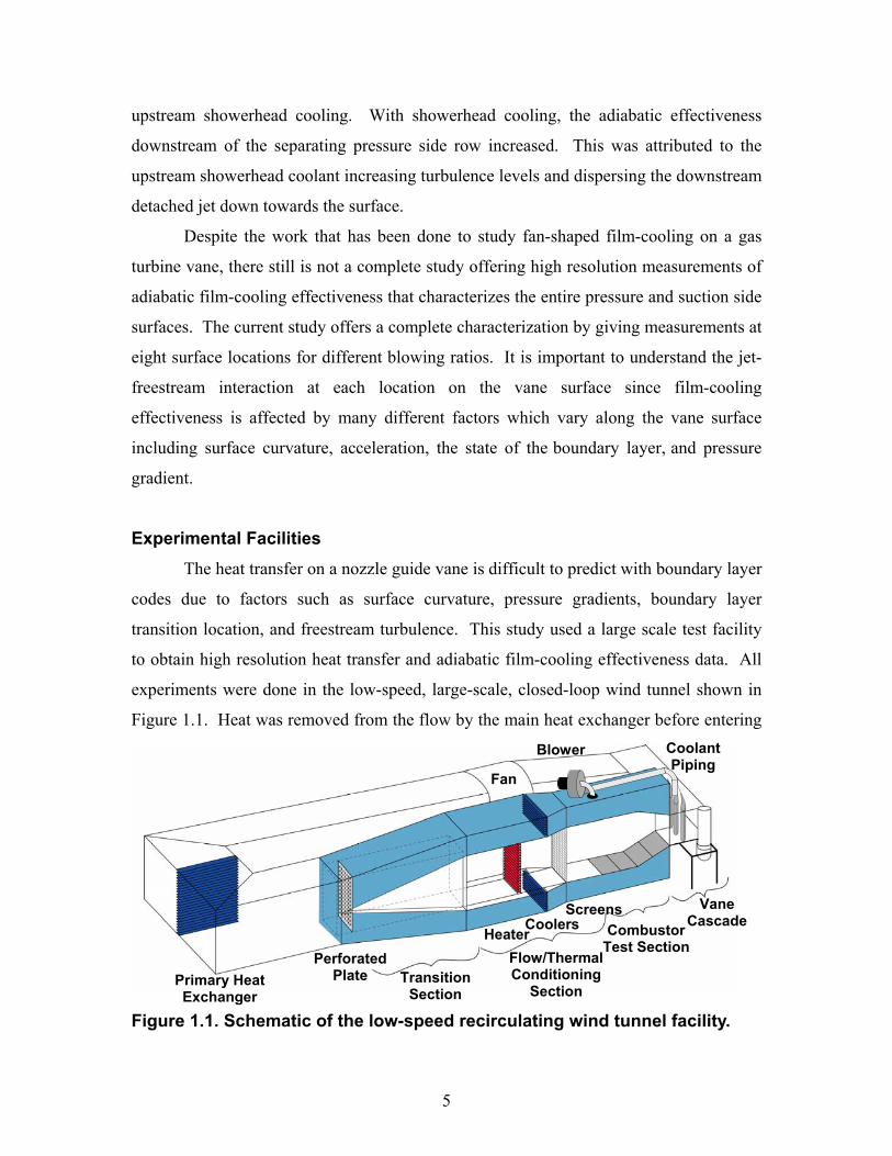
Experimental Facilities The heat transfer on a nozzle guide vane is difficult to predict with boundary layer

codes due to factors such as surface curvature, pressure gradients, boundary layer

transition location, and freestream turbulence. This study used a large scale test facility

to obtain high resolution heat transfer and adiabatic film-cooling effectiveness data. All

experiments were done in the low-speed, large-scale, closed-loop wind tunnel shown in

Figure 1.1. Heat was removed from the flow by the main heat exchanger before entering

Blower CoolantPiping

Fan

Primary Heat Exchanger

HeaterCoolers

Screens

Perforated Plate Transition

Section

Flow/Thermal Conditioning

Section

Combustor Test Section

Vane Cascade

Figure 1.1. Schematic of the low-speed recirculating wind tunnel facility.

6

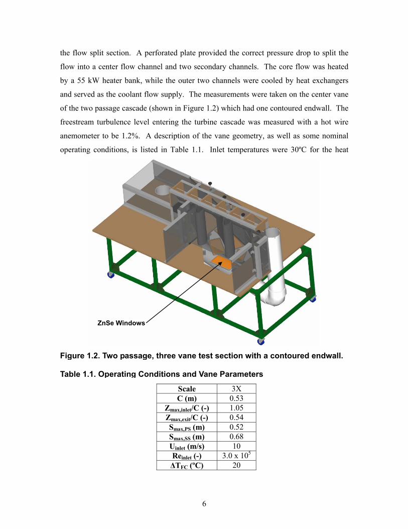
the flow split section. A perforated plate provided the correct pressure drop to split the

flow into a center flow channel and two secondary channels. The core flow was heated

by a 55 kW heater bank, while the outer two channels were cooled by heat exchangers

and served as the coolant flow supply. The measurements were taken on the center vane

of the two passage cascade (shown in Figure 1.2) which had one contoured endwall. The

freestream turbulence level entering the turbine cascade was measured with a hot wire

anemometer to be 1.2%. A description of the vane geometry, as well as some nominal

operating conditions, is listed in Table 1.1. Inlet temperatures were 30ºC for the heat

Scale 3X C (m) 0.53

Zmax,inlet/C (-) 1.05 Zmax,exit/C (-) 0.54 Smax,PS (m) 0.52 Smax,SS (m) 0.68 Uinlet (m/s) 10 Reinlet (-) 3.0 x 105 ∆TFC (ºC) 20

ZnSe Windows

Figure 1.2. Two passage, three vane test section with a contoured endwall.

Table 1.1. Operating Conditions and Vane Parameters

7

transfer coefficient tests and 60ºC for the film-cooling measurements, while inlet

pressures were nominally atmospheric.

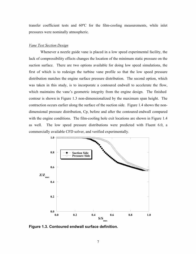
Vane Test Section Design

Whenever a nozzle guide vane is placed in a low speed experimental facility, the

lack of compressibility effects changes the location of the minimum static pressure on the

suction surface. There are two options available for doing low speed simulations, the

first of which is to redesign the turbine vane profile so that the low speed pressure

distribution matches the engine surface pressure distribution. The second option, which

was taken in this study, is to incorporate a contoured endwall to accelerate the flow,

which maintains the vane’s geometric integrity from the engine design. The finished

contour is shown in Figure 1.3 non-dimensionalized by the maximum span height. The

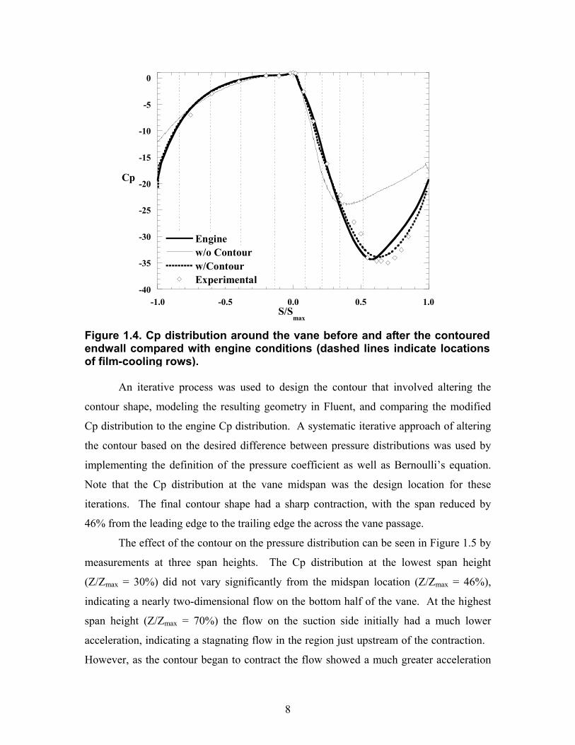
contraction occurs earlier along the surface of the suction side. Figure 1.4 shows the non-

dimensional pressure distribution, Cp, before and after the contoured endwall compared

with the engine conditions. The film-cooling hole exit locations are shown in Figure 1.4

as well. The low speed pressure distributions were predicted with Fluent 6.0, a

commercially available CFD solver, and verified experimentally.

0.0

0.2

0.4

0.6

0.8

1.0

0.0 0.2 0.4 0.6 0.8 1.0

Suction SidePressure Side

S/Smax

Z/Zmax

Figure 1.3. Contoured endwall surface definition.

8

-40

-35

-30

-25

-20

-15

-10

-5

0

-1.0 -0.5 0.0 0.5 1.0

Enginew/o Contourw/ContourExperimental

Cp

S/Smax

An iterative process was used to design the contour that involved altering the

contour shape, modeling the resulting geometry in Fluent, and comparing the modified

Cp distribution to the engine Cp distribution. A systematic iterative approach of altering

the contour based on the desired difference between pressure distributions was used by

implementing the definition of the pressure coefficient as well as Bernoulli’s equation.

Note that the Cp distribution at the vane midspan was the design location for these

iterations. The final contour shape had a sharp contraction, with the span reduced by

46% from the leading edge to the trailing edge the across the vane passage.

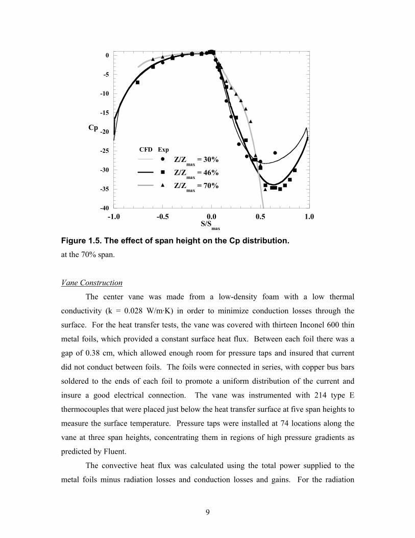
The effect of the contour on the pressure distribution can be seen in Figure 1.5 by

measurements at three span heights. The Cp distribution at the lowest span height

(Z/Zmax = 30%) did not vary significantly from the midspan location (Z/Zmax = 46%),

indicating a nearly two-dimensional flow on the bottom half of the vane. At the highest

span height (Z/Zmax = 70%) the flow on the suction side initially had a much lower

acceleration, indicating a stagnating flow in the region just upstream of the contraction.

However, as the contour began to contract the flow showed a much greater acceleration

Figure 1.4. Cp distribution around the vane before and after the contouredendwall compared with engine conditions (dashed lines indicate locations of film-cooling rows).

9

-40

-35

-30

-25

-20

-15

-10

-5

0

-1.0 -0.5 0.0 0.5 1.0

Z/Zmax

= 30%

Z/Zmax

= 46%

Z/Zmax

= 70%

Cp

S/Smax

CFD Exp

at the 70% span.

Vane Construction

The center vane was made from a low-density foam with a low thermal

conductivity (k = 0.028 W/m·K) in order to minimize conduction losses through the

surface. For the heat transfer tests, the vane was covered with thirteen Inconel 600 thin

metal foils, which provided a constant surface heat flux. Between each foil there was a

gap of 0.38 cm, which allowed enough room for pressure taps and insured that current

did not conduct between foils. The foils were connected in series, with copper bus bars

soldered to the ends of each foil to promote a uniform distribution of the current and

insure a good electrical connection. The vane was instrumented with 214 type E

thermocouples that were placed just below the heat transfer surface at five span heights to

measure the surface temperature. Pressure taps were installed at 74 locations along the

vane at three span heights, concentrating them in regions of high pressure gradients as

predicted by Fluent.

The convective heat flux was calculated using the total power supplied to the

metal foils minus radiation losses and conduction losses and gains. For the radiation

Figure 1.5. The effect of span height on the Cp distribution.

10

correction the emissivity, ε = 0.22, of the Inconel foils was assumed to be the same value

as stainless steel foils (Incropera and DeWitt [14]). The surrounding temperatures were

measured and found to agree with the freestream temperature. The radiation losses

amounted to 4% of the total heat flux. Conduction corrections were calculated based on a

one-dimensional conduction model driven by the temperature difference through the

foam vane and accounted for a maximum of about 2% of the total heat flux for the worst

case.

Adiabatic film-cooling effectiveness measurements were performed in the same

large-scale test facility as the heat transfer measurements. Coolant flow was provided by

the upper flow channel of the wind tunnel shown in Figure 1.1, using a blower to increase

the coolant supply pressure before it was fed into the film-cooling vane. The temperature

difference between the freestream and coolant flows was typically 20°C for the film-

cooling tests, yielding density ratios near 1.06. The center vane of the two passage

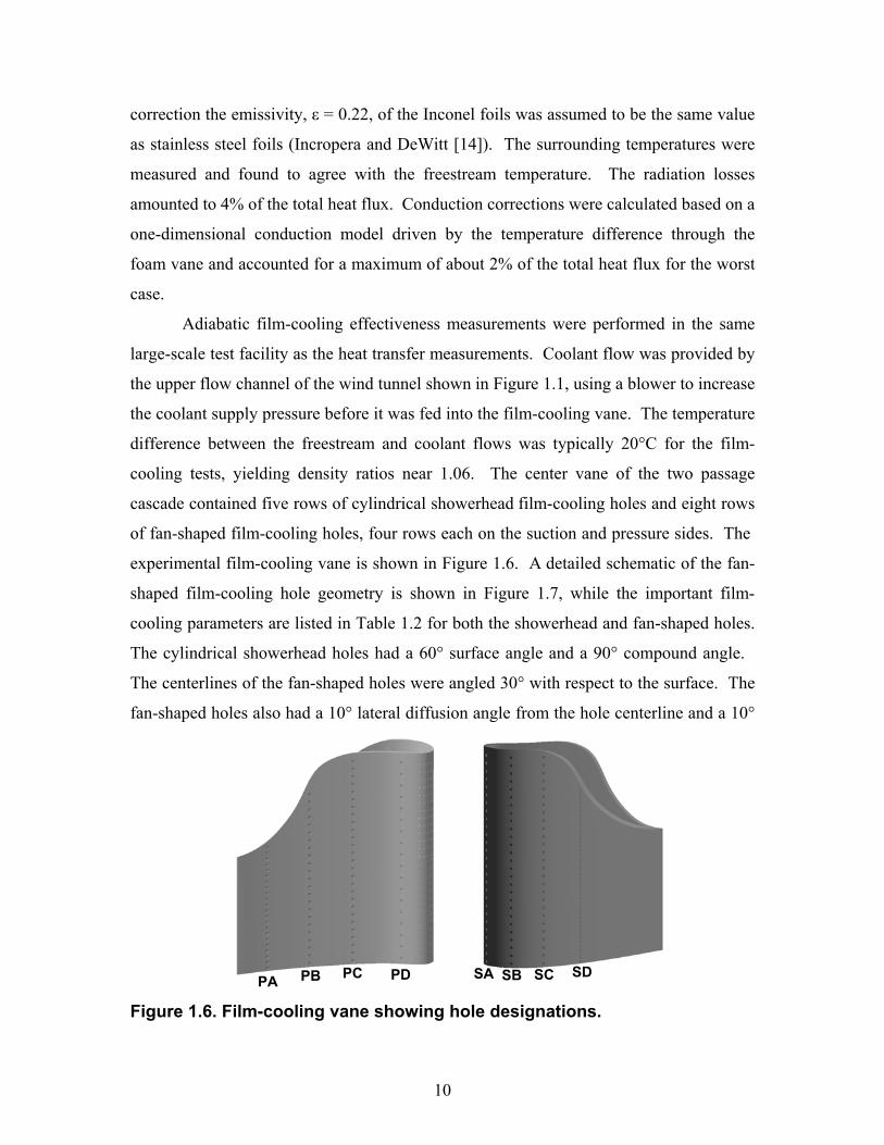
cascade contained five rows of cylindrical showerhead film-cooling holes and eight rows

of fan-shaped film-cooling holes, four rows each on the suction and pressure sides. The

experimental film-cooling vane is shown in Figure 1.6. A detailed schematic of the fan-

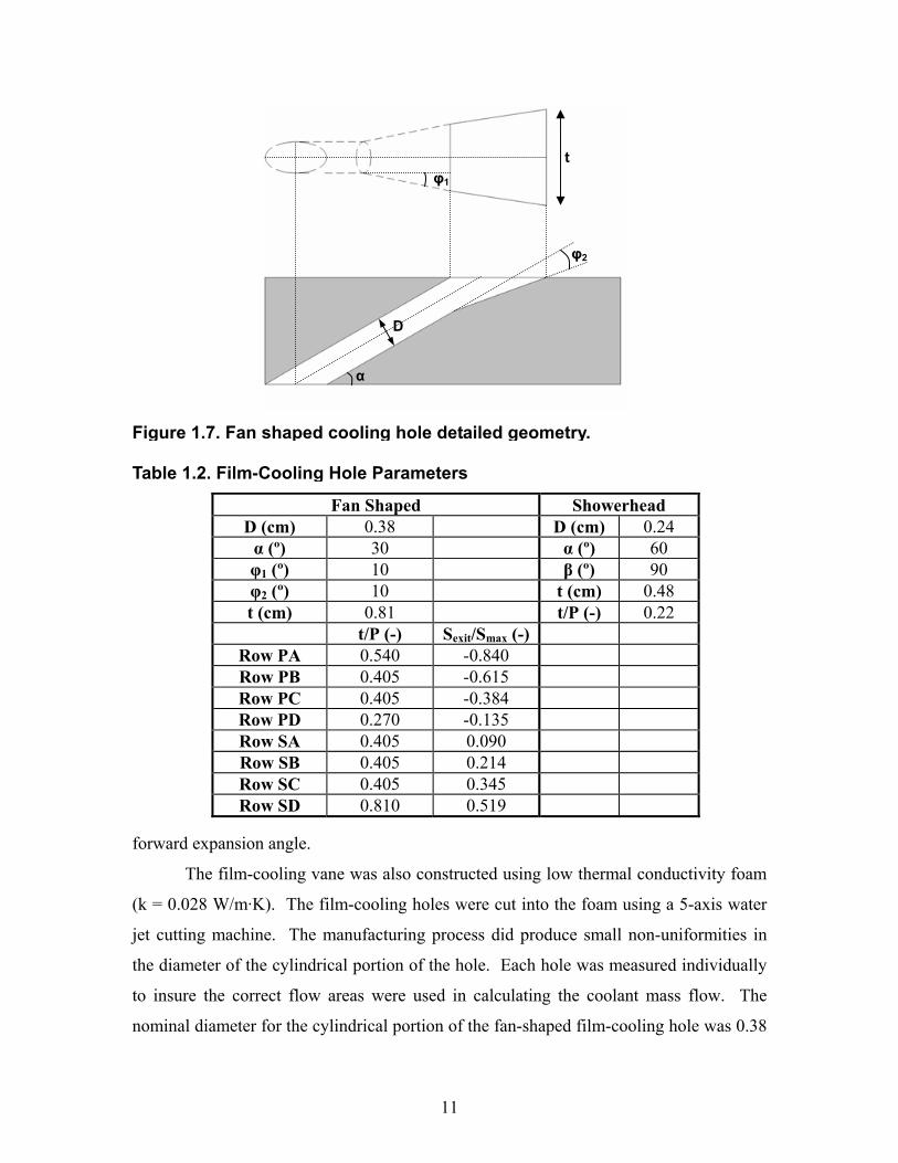
shaped film-cooling hole geometry is shown in Figure 1.7, while the important film-

cooling parameters are listed in Table 1.2 for both the showerhead and fan-shaped holes.

The cylindrical showerhead holes had a 60° surface angle and a 90° compound angle.

The centerlines of the fan-shaped holes were angled 30° with respect to the surface. The

fan-shaped holes also had a 10° lateral diffusion angle from the hole centerline and a 10°

PA PB PC PD SA SB SC SD

Figure 1.6. Film-cooling vane showing hole designations.

11

Fan Shaped Showerhead D (cm) 0.38 D (cm) 0.24 α (º) 30 α (º) 60 φ1 (º) 10 β (º) 90 φ2 (º) 10 t (cm) 0.48 t (cm) 0.81 t/P (-) 0.22

t/P (-) Sexit/Smax (-) Row PA 0.540 -0.840 Row PB 0.405 -0.615 Row PC 0.405 -0.384 Row PD 0.270 -0.135 Row SA 0.405 0.090 Row SB 0.405 0.214 Row SC 0.405 0.345 Row SD 0.810 0.519

forward expansion angle.

The film-cooling vane was also constructed using low thermal conductivity foam

(k = 0.028 W/m·K). The film-cooling holes were cut into the foam using a 5-axis water

jet cutting machine. The manufacturing process did produce small non-uniformities in

the diameter of the cylindrical portion of the hole. Each hole was measured individually

to insure the correct flow areas were used in calculating the coolant mass flow. The

nominal diameter for the cylindrical portion of the fan-shaped film-cooling hole was 0.38

D

α

φ2

φ1 t

Figure 1.7. Fan shaped cooling hole detailed geometry.

Table 1.2. Film-Cooling Hole Parameters

12

± 0.015 cm. Four plenums were placed inside the film-cooling vane to allow for the

capability of independently varying individual row blowing ratios. To verify to the non-

dimensional pressure distribution as discussed previously, pressure taps were placed at

46% span. Type E thermocouples were also placed flush with the surface at various

locations for calibration purposes.

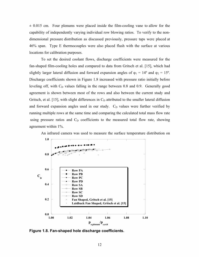
To set the desired coolant flows, discharge coefficients were measured for the

fan-shaped film-cooling holes and compared to data from Gritsch et al. [15], which had

slightly larger lateral diffusion and forward expansion angles of φ1 = 14º and φ2 = 15º.

Discharge coefficients shown in Figure 1.8 increased with pressure ratio initially before

leveling off, with CD values falling in the range between 0.8 and 0.9. Generally good

agreement is shown between most of the rows and also between the current study and

Gritsch, et al. [15], with slight differences in CD attributed to the smaller lateral diffusion

and forward expansion angles used in our study. CD values were further verified by

running multiple rows at the same time and comparing the calculated total mass flow rate

using pressure ratios and CD coefficients to the measured total flow rate, showing

agreement within 1%.

An infrared camera was used to measure the surface temperature distribution on

0.0

0.2

0.4

0.6

0.8

1.0

1.00 1.02 1.04 1.06 1.08 1.10

Row PARow PBRow PCRow PDRow SARow SBRow SCRow SDFan Shaped, Gritsch et al. [15]Laidback Fan Shaped, Gritsch et al. [15]

po,plenum

/ps,exit

CD

Figure 1.8. Fan-shaped hole discharge coefficients.

13

the vane during testing. Five images were taken at each location and averaged to

minimize experimental uncertainty. Images were taken from beneath the test section

through ZnSe windows placed in the lower flat endwall (illustrated in Figure 1.2). For

some of the rows, more than one image was necessary to capture the area downstream of

the cooling holes. Because of the vane surface curvature and the 45º angle between the

IR camera and the surface, the IR images needed to be transformed to accurately

represent the true surface distance. Prior to testing, a 1 cm x 1 cm grid was placed on the

surface of the vane and an IR image was taken at each viewing location. Next, the grid

vertices in each of the images were used to perform a 3rd or 4th order polynomial surface

transformation for that image.

The transformed images were then calibrated using type E thermocouples that

were placed flush with the vane surface. The infrared camera measures the radiation

from the surface, so an accurate knowledge of the surface emissivity and the surrounding

ambient temperature yield the correct surface temperature. The values of ε and Tamb for

each image were deduced by calibrating the image surface temperatures to match the

measured thermocouple temperatures over the full measurement range. Values for ε were

fairly consistent between image locations, varying from 0.6 to 0.7. The variation resulted

because not all of the images were taken at the same viewing angle or the same distance

from the surface.

Following the calibration procedure, the surface temperatures were non-

dimensionalized and corrected for conduction errors using the method established by

Ethridge et al. [16]. Values for ηo ranged from 0.04 to 0.12 around the vane surface,

where the highest values occurred just downstream of row PB on the pressure side.

Blowing ratios for this study were defined in two ways, depending on the region.

For the showerhead region, blowing ratios are reported based on the inlet velocity, Uin,

ininh

c

UAm

Mρ

=∞ (1.1)

However, for each row of fan-shaped holes, blowing ratios are reported in terms of the

local surface velocity, Ulocal,

inlocalh

c

UAm

Mρ

= (1.2)

14

Five blowing ratios were tested for the showerhead region, four blowing ratios

were tested for each row on the pressure side, and three blowing ratios were tested for

each row on the suction side. The range of blowing ratios was chosed to span typical

engine operating conditions.

Experimental Uncertainty

The partial derivative and sequential perturbation method given by Moffat [17]

were used to calculate uncertainties for the measured values. For a high reported value of

St = 0.0093 the uncertainty was ±3.23%, while the uncertainty for a low value of St =

0.0023 was ±2.13%. The uncertainties for the adiabatic effectiveness measurements were

±0.012 for a high value of ηAW = 0.9 and ±0.011 for a low value of ηAW = 0.2.

Experimental Results Heat transfer results will be discussed first followed by adiabatic effectiveness

results and a comparison to existing data from literature.

Heat Transfer Results

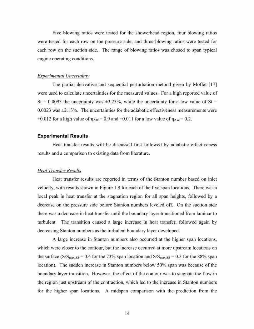
Heat transfer results are reported in terms of the Stanton number based on inlet

velocity, with results shown in Figure 1.9 for each of the five span locations. There was a

local peak in heat transfer at the stagnation region for all span heights, followed by a

decrease on the pressure side before Stanton numbers leveled off. On the suction side

there was a decrease in heat transfer until the boundary layer transitioned from laminar to

turbulent. The transition caused a large increase in heat transfer, followed again by

decreasing Stanton numbers as the turbulent boundary layer developed.

A large increase in Stanton numbers also occurred at the higher span locations,

which were closer to the contour, but the increase occurred at more upstream locations on

the surface (S/Smax,SS = 0.4 for the 73% span location and S/Smax,SS = 0.3 for the 88% span

location). The sudden increase in Stanton numbers below 50% span was because of the

boundary layer transition. However, the effect of the contour was to stagnate the flow in

the region just upstream of the contraction, which led to the increase in Stanton numbers

for the higher span locations. A midspan comparison with the prediction from the

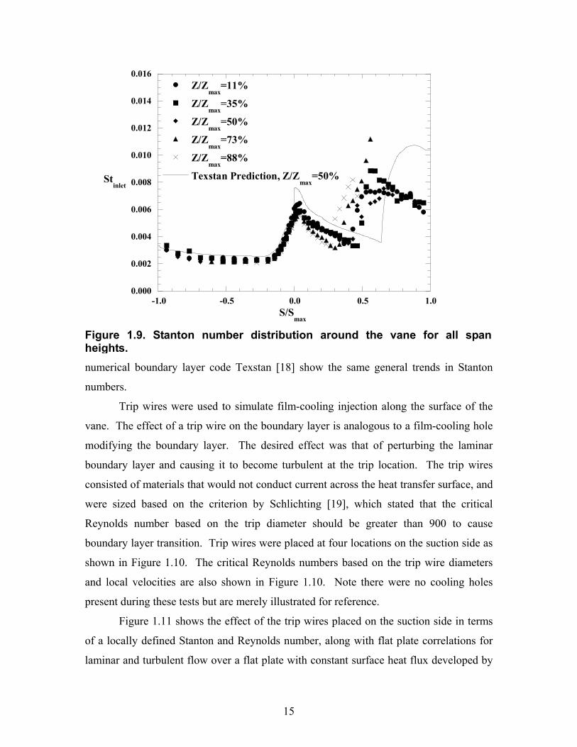
15

0.000

0.002

0.004

0.006

0.008

0.010

0.012

0.014

0.016

-1.0 -0.5 0.0 0.5 1.0

Z/Zmax

=11%

Z/Zmax

=35%

Z/Zmax

=50%

Z/Zmax

=73%

Z/Zmax

=88%

Texstan Prediction, Z/Zmax

=50%Stinlet

S/Smax

numerical boundary layer code Texstan [18] show the same general trends in Stanton

numbers.

Trip wires were used to simulate film-cooling injection along the surface of the

vane. The effect of a trip wire on the boundary layer is analogous to a film-cooling hole

modifying the boundary layer. The desired effect was that of perturbing the laminar

boundary layer and causing it to become turbulent at the trip location. The trip wires

consisted of materials that would not conduct current across the heat transfer surface, and

were sized based on the criterion by Schlichting [19], which stated that the critical

Reynolds number based on the trip diameter should be greater than 900 to cause

boundary layer transition. Trip wires were placed at four locations on the suction side as

shown in Figure 1.10. The critical Reynolds numbers based on the trip wire diameters

and local velocities are also shown in Figure 1.10. Note there were no cooling holes

present during these tests but are merely illustrated for reference.

Figure 1.11 shows the effect of the trip wires placed on the suction side in terms

of a locally defined Stanton and Reynolds number, along with flat plate correlations for

laminar and turbulent flow over a flat plate with constant surface heat flux developed by

Figure 1.9. Stanton number distribution around the vane for all span heights.

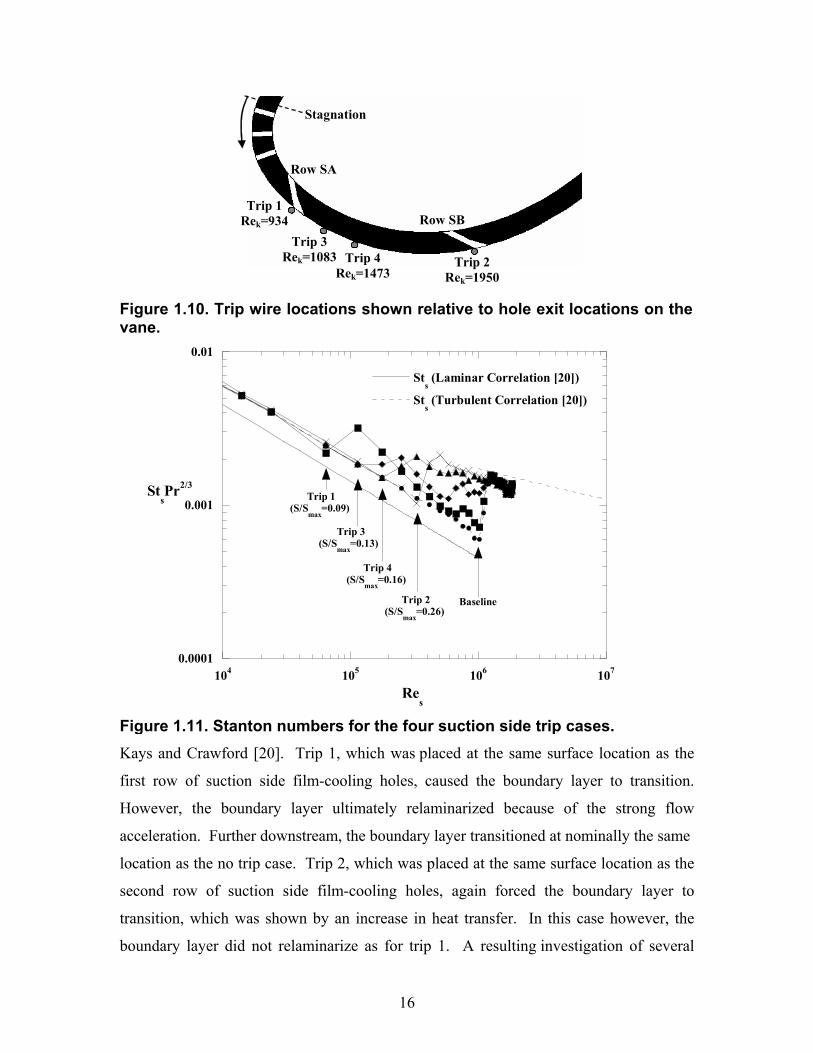
16

Row SA

Row SBTrip 1

Rek=934

Stagnation

Trip 3 Rek=1083 Trip 4

Rek=1473Trip 2

Rek=1950

0.0001

0.001

0.01

104 105 106 107

Sts (Laminar Correlation [20])

Sts (Turbulent Correlation [20])

StsPr2/3

Res

Trip 1(S/S

max=0.09)

Trip 3(S/S

max=0.13)

Trip 4(S/S

max=0.16)

Trip 2(S/S

max=0.26)

Baseline

Kays and Crawford [20]. Trip 1, which was placed at the same surface location as the

first row of suction side film-cooling holes, caused the boundary layer to transition.

However, the boundary layer ultimately relaminarized because of the strong flow

acceleration. Further downstream, the boundary layer transitioned at nominally the same

location as the no trip case. Trip 2, which was placed at the same surface location as the

second row of suction side film-cooling holes, again forced the boundary layer to

transition, which was shown by an increase in heat transfer. In this case however, the

boundary layer did not relaminarize as for trip 1. A resulting investigation of several

Figure 1.11. Stanton numbers for the four suction side trip cases.

Figure 1.10. Trip wire locations shown relative to hole exit locations on thevane.

17

more trip locations defined a critical region along the surface bounded by trips 3 and 4

wherein the boundary layer would transition to turbulent and not relaminarize.

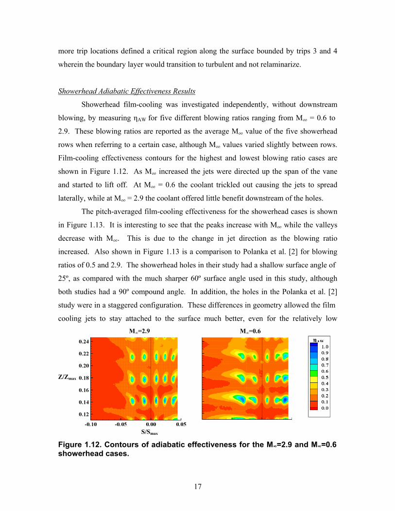
Showerhead Adiabatic Effectiveness Results

Showerhead film-cooling was investigated independently, without downstream

blowing, by measuring ηAW for five different blowing ratios ranging from M¶ = 0.6 to

2.9. These blowing ratios are reported as the average M¶ value of the five showerhead

rows when referring to a certain case, although M¶ values varied slightly between rows.

Film-cooling effectiveness contours for the highest and lowest blowing ratio cases are

shown in Figure 1.12. As M¶ increased the jets were directed up the span of the vane

and started to lift off. At M¶ = 0.6 the coolant trickled out causing the jets to spread

laterally, while at M¶ = 2.9 the coolant offered little benefit downstream of the holes.

The pitch-averaged film-cooling effectiveness for the showerhead cases is shown

in Figure 1.13. It is interesting to see that the peaks increase with M¶ while the valleys

decrease with M¶. This is due to the change in jet direction as the blowing ratio

increased. Also shown in Figure 1.13 is a comparison to Polanka et al. [2] for blowing

ratios of 0.5 and 2.9. The showerhead holes in their study had a shallow surface angle of

25º, as compared with the much sharper 60º surface angle used in this study, although

both studies had a 90º compound angle. In addition, the holes in the Polanka et al. [2]

study were in a staggered configuration. These differences in geometry allowed the film

cooling jets to stay attached to the surface much better, even for the relatively low M∞=2.9 M∞=0.6

ηAW

Z/Zmax

S/Smax

Figure 1.12. Contours of adiabatic effectiveness for the M∞=2.9 and M∞=0.6 showerhead cases.

18

0.0

0.1

0.2

0.3

0.4

0.5

0.6

0.7

0.8

-30.0 -22.5 -15.0 -7.5 0.0 7.5 15.0

Minf

=0.6

Minf

=1.0

Minf

=1.5

Minf

=2.0

Minf

=2.9

Minf

=0.50

Minf

=2.89

S/D

ηAW

α=60 degβ=90 deg

Polanka et al. [5]α=30 degβ=90 deg

blowing ratio of 0.5, leading to the much greater levels of laterally averaged effectiveness

by Polanka et al. [2].

Pressure Side Adiabatic Effectiveness Results

Single row adiabatic film-cooling effectiveness measurements were taken for four

rows on the pressure side, without any upstream showerhead blowing. Adiabatic

effectiveness contours for the highest (M = 7.4) and lowest (M = 2.9) blowing ratios

measured for the first pressure side row (Row PD: S/Smax,PS = -0.14) are shown in Figure

1.14. The contours for row PD show a contraction of the jet downstream of the hole exit

indicating jet separation. After about 10 hole diameters a large lateral spreading of the jet

occurs that yields an increase in both the level of adiabatic effectiveness and jet coverage.

Jet separation occurred immediately downstream of the hole location due to relatively

high local blowing ratios coupled with a concave surface curvature. However, as the

vane surface curved back into the jet trajectory, the jet impinged and spread onto the vane

surface. As expected, this phenomenon was accentuated with an increase in blowing

ratio, which led to increased separation. Also shown in Figure 1.14 is the laterally

averaged effectiveness for row PD. For this configuration, increased blowing led to

Figure 1.13. Laterally averaged effectiveness for the showerhead cases.

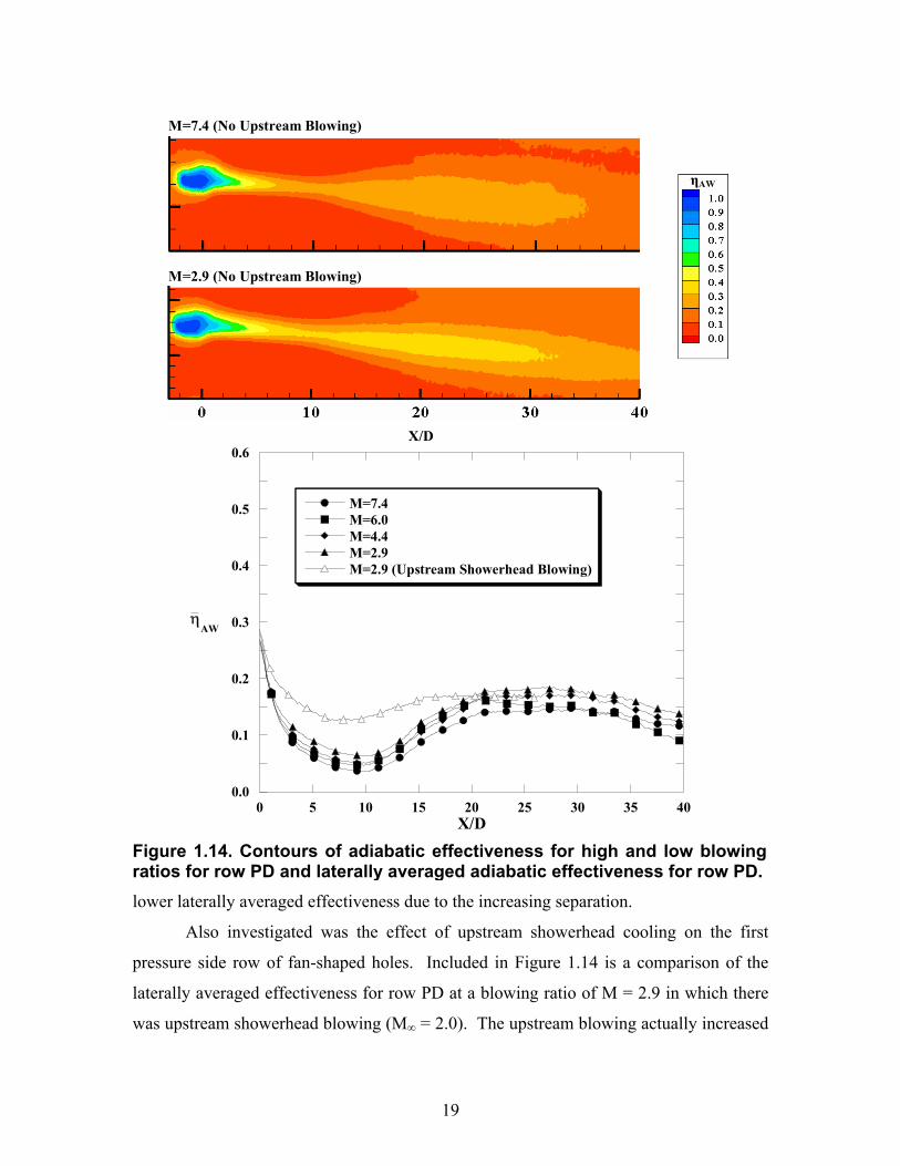
19

M=7.4 (No Upstream Blowing)

M=2.9 (No Upstream Blowing)

X/D

ηAW

0.0

0.1

0.2

0.3

0.4

0.5

0.6

0 5 10 15 20 25 30 35 40

M=7.4M=6.0M=4.4M=2.9M=2.9 (Upstream Showerhead Blowing)

X/D

ηAW

lower laterally averaged effectiveness due to the increasing separation.

Also investigated was the effect of upstream showerhead cooling on the first

pressure side row of fan-shaped holes. Included in Figure 1.14 is a comparison of the

laterally averaged effectiveness for row PD at a blowing ratio of M = 2.9 in which there

was upstream showerhead blowing (M∞ = 2.0). The upstream blowing actually increased

Figure 1.14. Contours of adiabatic effectiveness for high and low blowing ratios for row PD and laterally averaged adiabatic effectiveness for row PD.

20

the adiabatic effectiveness downstream of row PD. This is consistent with the findings of

Polanka et al. [13], who stated that for high blowing ratios the turbulence generated by

the upstream blowing tended to disperse the jet down onto the vane surface making it

more effective at cooling the surface.

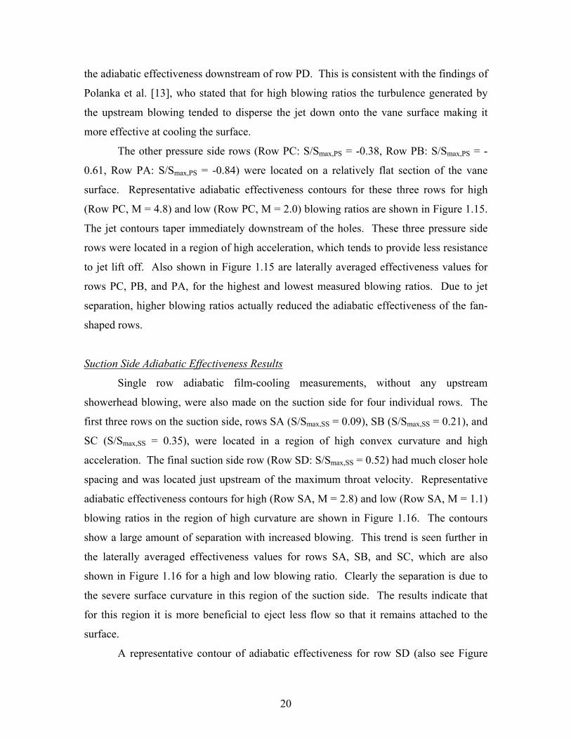
The other pressure side rows (Row PC: S/Smax,PS = -0.38, Row PB: S/Smax,PS = -

0.61, Row PA: S/Smax,PS = -0.84) were located on a relatively flat section of the vane

surface. Representative adiabatic effectiveness contours for these three rows for high

(Row PC, M = 4.8) and low (Row PC, M = 2.0) blowing ratios are shown in Figure 1.15.

The jet contours taper immediately downstream of the holes. These three pressure side

rows were located in a region of high acceleration, which tends to provide less resistance

to jet lift off. Also shown in Figure 1.15 are laterally averaged effectiveness values for

rows PC, PB, and PA, for the highest and lowest measured blowing ratios. Due to jet

separation, higher blowing ratios actually reduced the adiabatic effectiveness of the fan-

shaped rows.

Suction Side Adiabatic Effectiveness Results

Single row adiabatic film-cooling measurements, without any upstream

showerhead blowing, were also made on the suction side for four individual rows. The

first three rows on the suction side, rows SA (S/Smax,SS = 0.09), SB (S/Smax,SS = 0.21), and

SC (S/Smax,SS = 0.35), were located in a region of high convex curvature and high

acceleration. The final suction side row (Row SD: S/Smax,SS = 0.52) had much closer hole

spacing and was located just upstream of the maximum throat velocity. Representative

adiabatic effectiveness contours for high (Row SA, M = 2.8) and low (Row SA, M = 1.1)

blowing ratios in the region of high curvature are shown in Figure 1.16. The contours

show a large amount of separation with increased blowing. This trend is seen further in

the laterally averaged effectiveness values for rows SA, SB, and SC, which are also

shown in Figure 1.16 for a high and low blowing ratio. Clearly the separation is due to

the severe surface curvature in this region of the suction side. The results indicate that

for this region it is more beneficial to eject less flow so that it remains attached to the

surface.

A representative contour of adiabatic effectiveness for row SD (also see Figure

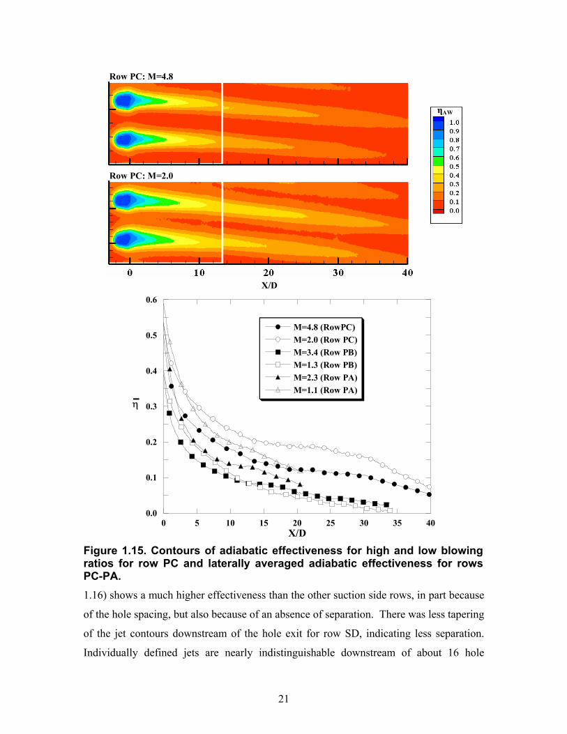
21

Row PC: M=4.8

Row PC: M=2.0

X/D

ηAW

0.0

0.1

0.2

0.3

0.4

0.5

0.6

0 5 10 15 20 25 30 35 40

M=4.8 (RowPC)M=2.0 (Row PC)M=3.4 (Row PB)M=1.3 (Row PB)M=2.3 (Row PA)M=1.1 (Row PA)

X/D

η

1.16) shows a much higher effectiveness than the other suction side rows, in part because

of the hole spacing, but also because of an absence of separation. There was less tapering

of the jet contours downstream of the hole exit for row SD, indicating less separation.

Individually defined jets are nearly indistinguishable downstream of about 16 hole

Figure 1.15. Contours of adiabatic effectiveness for high and low blowing ratios for row PC and laterally averaged adiabatic effectiveness for rowsPC-PA.

22

Row SA: M=2.8

Row SA: M=1.1

X/D Row SD: M=0.8

X/D

ηAW

0.0

0.2

0.4

0.6

0.8

1.0

0 5 10 15 20 25 30 35 40

M=2.8 (Row SA)M=1.1 (Row SA)M=1.8 (Row SB)M=0.9 (Row SB)M=1.5 (Row SC)M=0.9 (Row SC)M=1.2 (Row SD)M=0.8 (Row SD)

X/D

ηAW

Figure 1.16. Contours of adiabatic effectiveness for high and low blowingratios for row SA and a representative case for row SD. Also laterally averaged effectiveness for the suction side rows.

23

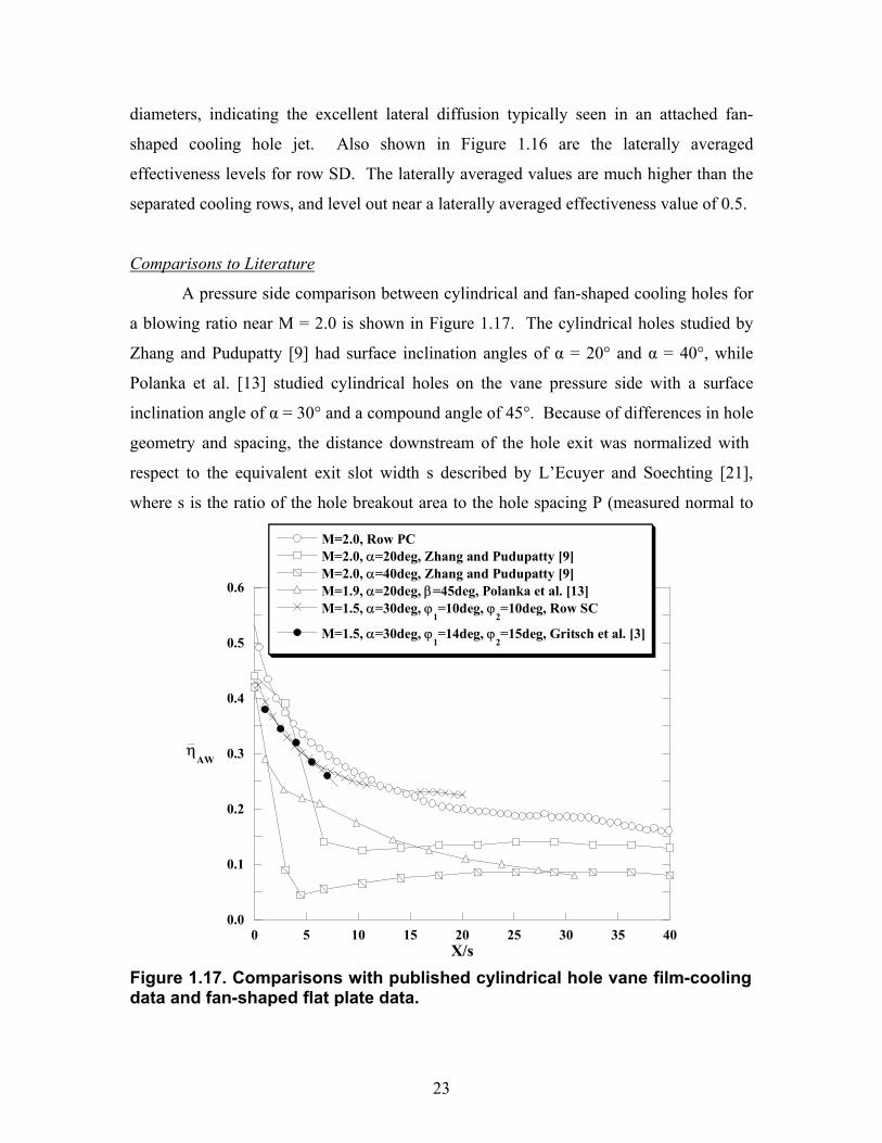
diameters, indicating the excellent lateral diffusion typically seen in an attached fan-

shaped cooling hole jet. Also shown in Figure 1.16 are the laterally averaged

effectiveness levels for row SD. The laterally averaged values are much higher than the

separated cooling rows, and level out near a laterally averaged effectiveness value of 0.5.

Comparisons to Literature

A pressure side comparison between cylindrical and fan-shaped cooling holes for

a blowing ratio near M = 2.0 is shown in Figure 1.17. The cylindrical holes studied by

Zhang and Pudupatty [9] had surface inclination angles of α = 20° and α = 40°, while

Polanka et al. [13] studied cylindrical holes on the vane pressure side with a surface

inclination angle of α = 30° and a compound angle of 45°. Because of differences in hole

geometry and spacing, the distance downstream of the hole exit was normalized with

respect to the equivalent exit slot width s described by L’Ecuyer and Soechting [21],

where s is the ratio of the hole breakout area to the hole spacing P (measured normal to

0.0

0.1

0.2

0.3

0.4

0.5

0.6

0 5 10 15 20 25 30 35 40

M=2.0, Row PCM=2.0, α=20deg, Zhang and Pudupatty [9]M=2.0, α=40deg, Zhang and Pudupatty [9]M=1.9, α=20deg, β=45deg, Polanka et al. [13]M=1.5, α=30deg, ϕ

1=10deg, ϕ

2=10deg, Row SC

M=1.5, α=30deg, ϕ1=14deg, ϕ

2=15deg, Gritsch et al. [3]

X/s

ηAW

Figure 1.17. Comparisons with published cylindrical hole vane film-cooling data and fan-shaped flat plate data.

24

the streamwise direction). This comparison shows that the fan-shaped hole geometry

offers a significant increase in adiabatic effectiveness over cylindrical holes.

Although there has been some previous studies done with fan-shaped holes on a

vane surface, it was not possible to make a direct comparison to these studies, as the

equivalent slot width was not able to be determined. For a region on the suction side with

relatively low surface curvature, a comparison was made between data from our study

and fan-shaped data on a flat plate from Gritsch et al. [3] (also shown in Figure 1.17).

The flat plate study by Gritsch et al. [3] featured the same surface inclination angle as our

study (α = 30°), with slightly larger lateral diffusion and forward expansion angles of φ1

= 14º and φ2 = 15º. In this region of relatively low surface curvature on the suction side,

very good agreement is shown just downstream of the hole between the current study and

the flat plate study by Gritsch et al. [3].

Conclusions This paper has presented a coupled study of the heat transfer coefficients and

adiabatic effectiveness for a large-scale turbine vane under low-speed conditions. A

contoured endwall was designed in order to match the engine pressure distribution around

the vane. Heat transfer results showed a peak in Stanton numbers near the leading edge.

Stanton numbers decreased on the pressure side to a constant value. On the suction side,

Stanton numbers decreased until a surface location of S/Smax = 0.5, where Stanton

numbers were increased because of the boundary layer transitioning from laminar to

turbulent.

Trip wires were used to simulate the boundary layer transition caused by film-

cooling holes on the vane suction side. It was noted that using a trip wire to transition the

boundary layer increased the Stanton numbers as if the boundary layer had transitioned

naturally. The trip wire placed at the location of the first film-cooling hole row tripped

the boundary layer, but the boundary layer relaminarized before the natural transition

location. An investigation of trip wire location showed the sensitivity to location in terms

of the boundary layer transition and the relaminarizing process. This sensitivity should

be considered by engine designers when determining film-cooling hole placement, as this

will dictate the laminar to turbulent boundary layer transition.

25

Adiabatic effectiveness measurements for the showerhead region showed that

increasing the blowing ratio changed the direction of the jets and reduced the amount of

lateral spreading. Adiabatic film-cooling effectiveness measurements showed that in

regions of high curvature just downstream of the leading edge the jets separated from the

surface. However, on the pressure side where there was a concave surface curvature near

the first cooling hole row, the coolant jets impinged on the surface about ten hole

diameters downstream and spread laterally. Along both the suction and pressure sides,

increasing the blowing ratio tended to accentuate the jet lift off, reducing overall film-

cooling effectiveness. The presence of upstream showerhead blowing on the first

pressure side row tended to increase the turbulent diffusion of the jet downwards onto the

surface, increasing effectiveness. The suction side was particularly hard to cool due to

the jet separation resulting from the convex curvature.

A comparison to previous cylindrical hole vane cooling studies further highlights

the cooling benefit from fan-shaped holes over the traditional cylindrical cooling hole

shape. This study emphasizes the difficulty of film-cooling hole placement, as there are

many effects that play a role in the effectiveness of a cooling jet. These effects include

boundary layer transition location, surface curvature, acceleration, hole spacing, and

blowing ratio.

Acknowledgments The authors are grateful to Siemens Power Generation for their funding and

support of this project.

Nomenclature A area

C vane chord

CD discharge coefficient

Cp specific heat

Cp static pressure coefficient, Cp = (ps,local – ps,in)/0.5ρinU2in

D film-cooling hole diameter

h heat transfer coefficient

26

k thermal conductivity

m mass flow rate

M blowing ratio using local velocity, mc/AhUlocalρin

M∞ blowing ratio using inlet velocity, mc/AhUinρin

p pressure

P hole spacing measured normal to streamwise direction

Re Reynolds number, Re = UinC/υ

s equivalent slot width, Abreak/P

S distance along the vane surface

Stin Stanton number using inlet conditions, Stin = h/ρinCpUin

Sts Stanton number using local conditions, Sts = h/ρinCpUlocal

t hole breakout width

U velocity

X distance downstream of the hole exit

Z distance measured along the vane span

Greek

α inclination angle

β compound angle

ε surface emissivity

ηAW adiabatic film-cooling effectiveness, ηAW = (ηmeas – ηo)/(1 – ηo)

ηmeas effectiveness with blowing, ηmeas = (T∞ – Tsurf)/(T∞ – Tc)

ηo effectiveness without blowing, ηo = (T∞ – Tsurf)/(T∞ – Tc)

ρ density

υ kinematic viscosity

φ1 lateral diffusion angle

φ2 forward expansion angle

Subscripts

amb ambient

break hole breakout area

27

c coolant

h metering area of film-cooling holes based on D

in inlet condition

k critical

local local conditions

max maximum

o total

s static pressure

surf surface

∞ freestream conditions

Overbar

– lateral average

References [1] Riess, H., and Bölcs, A., 2000, “The Influence of the Boundary Layer State and

Reynolds Number on Film-cooling and Heat Transfer on a Cooled Nozzle Guide

Vane,” 2000-GT-205.

[2] Polanka, M. D., Witteveld, V. C., and Bogard, D. G., 1999, “Film-cooling

Effectiveness in the Showerhead Region of a Gas Turbine Vane Part 1: Stagnation

Region and Near Pressure Side,” 99-GT-48.

[3] Gritsch, M., Schulz, A., and Wittig, S., 1998, “Adiabatic Wall Effectiveness

Measurements of Film-Cooling Holes with Expanded Exits,” ASME Journal of

Turbomachinery, vol. 120, pp. 549.

[4] Yuen, C. H. N., Martinez-Botas, R. F., and Whitelaw, J. H., 2001, “Film-cooling

Effectiveness Downstream of Compound and Fan-Shaped Holes,” 2001-GT-0131.

[5] Dittmar, J., Schulz, A., and Wittig, S., 2002, “Assessment of Various Film-

28

cooling Configurations Including Shaped and Compound Angle Holes Based on

Large Scale Experiments,” GT-2002-30176.

[6] Dittmar, J., Schulz, A., and Wittig, S., 2004, “Adiabatic Effectiveness and Heat

Transfer Coefficient of Shaped Film-cooling Holes on a Scaled Guide Vane

Pressure Side Model,” International Journal of Rotating Machinery, vol. 10, pp.

345-354.

[7] Guo, S. M., Lai, C. C., Jones, T. V., Oldfield, M. L. G., Lock, G. D., and

Rawlinson, A. J., 1998, “The Application of Thin-Film Technology to Measure

Turbine-Vane Heat Transfer and Effectiveness in a Film-Cooled, Engine-

Simulated Environment,” International Journal of Heat and Fluid Flow, vol. 19,

pp. 594-600.

[8] Zhang, L., Baltz, M., Pudupatty, R., and Fox, M., 1999, “Turbine Nozzle Film-

cooling Study Using the Pressure Sensitive Paint (PSP) Technique,” 99-GT-196.

[9] Zhang, L., and Pudupatty, R., 2000, “The Effects of Injection Angle and Hole

Exit Shape on Turbine Nozzle Pressure Side Film-cooling,” 2000-GT-247.

[10] Sargison, J. E., Guo, S. M., Oldfield, M. L. G., Lock, G. D., and Rawlinson, A. J.,

2001, “A Converging Slot-Hole Film-Cooling Geometry Part 1: Low-Speed Flat-

Plate Heat Transfer and Loss,” 2001-GT-0126.

[11] Sargison, J. E., Guo, S. M., Oldfield, M. L. G., Lock, G. D., and Rawlinson, A. J.,

2001, “A Converging Slot-Hole Film-Cooling Geometry Part 2: Transonic Nozzle

Guide Vane Heat Transfer and Loss,” 2001-GT-0127.

[12] Schneider, M., Parneix, S., and von Wolfersdorf, J., 2003, “Effect of Showerhead

Injection on Superposition of Multi-Row Pressure Side Film-cooling with Fan-

shaped Holes,” GT-2003-38693.

29

[13] Polanka, M. D., Ethridge, M. I., Cutbirth, J. M., and Bogard, D. G., 2000, “Effects

of Showerhead Injection on Film-cooling Effectiveness for a Downstream Row of

Holes,” 2000-GT-240.

[14] Incropera, F. P., and DeWitt, D. P., 1996, Fundamentals of Heat and Mass

Transfer, 4th ed., New York: J. Wiley & Sons.

[15] Gritsch, M., Schulz, A., and Wittig, S., 1997, “Discharge Coefficient

Measurements of Film-Cooling Holes with Expanded Exits,” 97-GT-165.

[16] Ethridge, M. I., Cutbirth, J. M., and Bogard, D. G., 2000, “Scaling of Performance

for Varying Density Ratio Coolants on an Airfoil with Strong Curvature and

Pressure Gradient Effects,” 2000-GT-239.

[17] Moffat, R. J., 1988, “Describing the Uncertainties in Experimental Results,”

Experimental Thermal and Fluid Science, vol. 1, pp. 3-17.

[18] Crawford, M. E., 1986, “Simulation Codes for Calculation of Heat Transfer to

Convectively-Cooled Turbine Blades,” 130 pp., a set of four lectures in

Convective Heat Transfer and Film-cooling in Turbomachinery, T. Arts, ed.,

Lecture Series 1986-06, von Karman Institute for Fluid Dynamics, Rhode-Saint-

Genese, Belgium.

[19] Schlichting, H., 1979, Boundary Layer Theory, 7th Edition, McGraw-Hill, New

York.

[20] Kays, W. M., and Crawford, M. E., 1991, Convective Heat and Mass Transfer,

McGraw-Hill, New York.

[21] L’Ecuyer, M. R., and Soechting, F. O., 1985, “A Model for Correlating Flat Plate

Film-cooling Effectiveness for Rows of Round Holes,” Heat Transfer and

30

Cooling in Gas Turbines, AGARD CP-390, Paper 19.

* Co-authors: Dr. Karen A. Thole, Mechanical Engineering Department, Virginia Tech Michael Haendler, Siemens Power Generation, Muelheim a. d. Ruhr, Germany

Paper 2: Experimental and Computational Comparisons of Fan-Shaped

Film-Cooling on a Turbine Vane Surface

Accepted for publication in the ASME Journal of Turbomachinery*

Abstract The flow exiting the combustor in a gas turbine engine is considerably hotter than

the melting temperature of the turbine section components, of which the turbine nozzle

guide vanes see the hottest gas temperatures. One method used to cool the vanes is to use

rows of film-cooling holes to inject bleed air that is lower in temperature through an array

of discrete holes onto the vane surface. The purpose of this study was to evaluate the

row-by-row interaction of fan-shaped holes as compared to the performance of a single

row of fan-shaped holes in the same locations.

This study presents adiabatic film-cooling effectiveness measurements from a

scaled-up, two-passage vane cascade. High resolution film-cooling measurements were

made with an infrared (IR) camera at a number of engine representative flow conditions.

Computational fluid dynamics (CFD) predictions were also made to evaluate the

performance of some of the current turbulence models in predicting a complex flow such

as turbine film-cooling. The RNG k-ε turbulence model gave a closer prediction of the

overall level of film-effectiveness, while the v2-f turbulence model gave a more accurate

representation of the flow physics in some regions.

32

Introduction The nozzle guide vanes in a gas turbine, located directly downstream of the

combustion section, are particularly susceptible to thermal failure, with gas temperatures

commonly reaching levels above component latent melting temperatures. Combustion

temperatures continue to rise in an effort to increase the efficiency and power output from

gas turbine engines. This rise has led to the increased demand to devise better cooling

schemes and more resilient materials from which to manufacture the turbine vanes.

Many cooling strategies are typically used at the same time; including impingement

cooling, internal passage cooling, and external film-cooling. While designing various

cooling configurations, consideration must also be given to the structural integrity of the

vanes, since turbine vanes are under extremely high thermal stresses.

Ideally, film-cooling aims to inject cooler temperature fluid over the surface of

the vane, shielding it from the high temperature freestream gases. This goal is sometimes

difficult to achieve, however, as the nature of the flow through the turbine passage tends

to be uncompromising with conditions including high freestream turbulence, secondary

flows, high surface curvature, rapid flow acceleration, and high pressure gradients, all of

which have been shown to affect cooling performance. Film-cooling offers the engine

designer an enticing way to extend part life, however, the use of too much coolant flow

from the compressor takes a toll on the overall engine efficiency. To counteract this

consequence, engine designers are constantly on the lookout for ways to maintain or even

increase the cooling performance but with less coolant.

Alternative hole geometries are sometimes used by engine designers, such as the

diffused or so-called fan-shaped holes, to maximize the performance of the injected

coolant. By expanding the exit of the cooling hole in the lateral direction, the effective

momentum of the surface coolant can be reduced prior to injection. Goldstein et al. [1]

showed that fan-shaped holes provide better surface attachment at higher blowing ratios,

as well as better lateral spreading of the coolant than cylindrical holes. A slight deviation

of this design is the laidback fan-shaped hole, wherein a forward expansion is also

included, further inhibiting jet liftoff. The major drawback for non-cylindrical hole

geometries is increased initial manufacturing costs. The benefits however, of fan-shaped

holes are many, including increased part life (fewer replacements needed), less required

33

coolant (increased engine efficiency), and fewer holes needed (increased structural

stability of the vane).

CFD is becoming an essential design tool in the gas turbine industry, because it is

both cheaper and faster than performing experiments. However, in order to rely on CFD

results it is first necessary to validate the predictions with measurements to ensure

computational reliability. In this study, detailed comparisons of the measured adiabatic

effectiveness data are made with CFD predictions using both the RNG k-ε and v2-f

turbulence models.

The standard k-ε turbulence model is a Reynolds Averaged Navier-Stokes

(RANS) model with two transport equations – one for the turbulent kinetic energy (k) and

one for the eddy viscosity (ε) – which are used to approximate the turbulent viscosity (µt).

The RNG k-ε model involves renormalization group theory and adds a term to the eddy

viscosity transport equation, which makes the model better for high strain flows than the

standard k-ε model. One major drawback of the RNG k-ε model in wall-bounded flows

such as film-cooling is the assumption of isotropic turbulence. The existence of the wall

introduces anisotropy in the normal fluctuations, the presence of which are not accounted

for in the wall functions used to approximate the behavior in the boundary layer in the k-ε

turbulence models. Wall functions lose their reliability in 3D or separated flow regimes

such as sometimes seen in film-cooling.

Durbin [2] incorporated turbulence anisotropy in the near wall region into the

existing k-ε RANS model by adding two transport equations – one for the normal

fluctuations (v2) and one for an elliptic relaxation function (f) – and effectively removed

the necessity of wall functions. The v2-f turbulence model correctly models the blocking

phenomenon near the wall that is responsible for attenuating the normal turbulent

fluctuations, eliminating the requirement of damping functions in wall bounded flows.

Film-cooling effectiveness has been predicted using both the RNG k-ε and the v2-

f turbulence models in our paper. The complete passage, including the contoured

endwall was modeled in the RNG k-ε simulation for a baseline case. A spanwise

periodic section of the vane passage was modeled using the v2-f turbulence model for the

same blowing ratios that were measured experimentally.

This study is the first to present detailed high-resolution adiabatic film-cooling

34

effectiveness measurements for a turbine vane with multiple rows of fan-shaped film-

cooling holes at engine representative blowing ratios. Contours and laterally averaged

values of adiabatic film-cooling effectiveness are presented for both the pressure and

suction sides. Adiabatic film-cooling effectiveness data is critical information for engine

designers, necessary to predict not only metal temperatures but also to validate CFD

predictions.

Past Studies Because of its crucial role in preventing thermal failure in gas turbine engines,

film-cooling has been an extensively researched topic over the last 30 to 35 years

([3],[4]). Flat plate studies have encompassed a variation of every possible geometrical

parameter; including surface angle, entrance length, hole spacing, compound angle,

lateral expansion angle, forward expansion angle, area ratio, and multiple row

configurations. External conditions have also been thoroughly investigated for flat

plates; including such effects as turbulence intensity, pressure gradient, and the state of

the approaching boundary layer. An excellent review of the relevant shaped hole

literature, which primarily focused on flat-plate studies, was given by Bunker [5].

Although flat plate studies are a key first step in understanding the flow physics for a

given cooling hole geometry, to completely understand the flow physics and evaluate a

given film-cooling design, it must be tested on the actual turbine vane. It stands to reason

that the flow physics on a highly curved surface such as a turbine vane, coupled with

multiple cooling row interaction, could yield results that are different from the flat plate

special case. Some studies have presented results for partially and/or fully cooled nozzle

guide vanes, but the deficiency of many of those studies is the lack of high resolution

effectiveness measurements.

Studies involving a single row of fan-shaped cooling holes on a vane surface have

been performed by Zhang et al. [6], Zhang and Pudupatty [7], and Colban et al. [8].

Using the same experimental procedure and facilities for both studies, effectiveness

measurements were made with fan-shaped holes on the suction side by Zhang et al. [6]

and on the pressure side by Zhang and Pudupatty [7]. Results indicated an increase in

effectiveness on the suction side for the blowing ratio range from 0.5 to 1.5 and a

35

decrease in effectiveness on the pressure side for the blowing ratio range from 1.5 to 2.5.

Colban et al. [8] presented adiabatic effectiveness measurements for eight single rows of

fan-shaped holes on both the pressure and suction sides in the same facilities as this paper.

Their results indicated that in regions of high convex curvature, particularly on the

suction side near the leading edge, jet lift-off was prevalent, and increased with blowing

ratio. Colban et al. [8] also noted a decrease in effectiveness with increased blowing on

the pressure side, which was attributed to partial jet lift-off and hot gas entrainment.

Despite the knowledge gained by studying single row cooling on the vane, it is

still necessary to study multiple row film-cooling on the vane. Goldstein et al. [9]

showed that on a flat plate a single row of cooling holes separated with increasing

blowing ratio, resulting in decreased film-effectiveness. However, with a double row

cooling configuration, the upstream row provided the impetus for the downstream row to

stay attached to the surface. This resulted in an increased film-effectiveness with

blowing ratio. The study by Goldstein et al. [9] suggested that an accurate study of vane

film-cooling would not be complete unless all of the engine-present film-cooling rows

were tested together.

Effectiveness measurements were made by Guo et al. [10] in a transonic facility

for a turbine airfoil with multiple rows of fan-shaped holes. Results showed higher

values of effectiveness for fan-shaped holes than for cylindrical holes. However, the

decay in effectiveness on the pressure side was faster for fan-shaped than for cylindrical

holes, which was most likely the result of a better lateral coverage for the fan-shaped

holes. Sargison et al. [11] also measured effectiveness in an annular turbine cascade with

multiple rows of cylindrical, fan-shaped, and converging slot holes. They reported

similar levels of performance for the fan-shaped and converging slot holes, both of which

had superior performance than cylindrical holes.

Effectiveness measurements on the pressure side were made for three rows of fan-

shaped holes and isothermal showerhead blowing by Schnieder et al. [12]. They reported

that the presence of isothermal showerhead blowing caused increased mixing of the first

pressure side row, lowering effectiveness. However, with showerhead cooling, perhaps

the increased mixing of the first pressure side row might actually improve effectiveness.

Polanka et al. [13] also studied the effect of showerhead blowing on the first downstream

36

pressure side row, using cylindrical instead of fan-shaped holes. They reported that

showerhead blowing caused the jets to stay attached, where they would normally separate

without upstream blowing. Polanka et al. [13] suggested that increased turbulent mixing

caused by the showerhead dispersed the jet towards the wall, reducing lift-off.

Colban et al. [8] presented effectiveness for fan-shaped holes combined with

upstream showerhead blowing. Their results indicated that upstream showerhead

blowing increased jet dispersion towards the vane surface for the first row of film-cooling

holes downstream on the pressure side, a result consistent with the results of Polanka et al.

[13]. Although Colban et al. [8] presented a complete set of high resolution data for

single row fan-shaped holes on a turbine vane, it is further necessary to understand the

row-to-row interaction, as the state of the approaching boundary layer has been shown to

have a significant effect on the performance of a film-cooling jet [14].

There have been a limited number of computational studies involving shaped hole

film-cooling on a flat plate. Kohli and Thole [15] used the standard k-ε model with non-

equilibrium wall functions to show the importance of modeling the interior plenum

conditions correctly. A similar flat-plate study was performed by Hyams and Leylek [16]

who investigated the effect of hole geometry on the thermal and flow field using the high

Reynolds number k-ε model with generalized wall functions. They showed that laterally

diffused shaped holes had the highest adiabatic effectiveness levels downstream of the

hole exit location.

Computational film-cooling studies on a turbine vane surface with fan-shaped

holes have been done by Hildebrandt et al. [17], Ferguson et al. [18] and Heidmann et al.

[19]. Only Heidmann et al. [19] however, modeled more than one row of holes on the

vane. Their study used the k-ω model to simulate a periodic section of the vane with six

staggered rows of cylindrical showerhead holes, four rows of fan-shaped holes on the

pressure side, and two rows of cylindrical holes on the suction side. The numerical

results presented by Heidmann et al. [19] were not validated with experiments, so the

validity of the method was not established. The single row numerical results of Ferguson

et al. [18] showed good agreement with experimental results for blowing ratios less than

1.5 using the RNG k-ε model with a two-layer wall treatment. Above a blowing ratio of

1.5, the agreement was not so good.

37

Nothing, to the author’s knowledge, as of yet has been published applying the v2-f

turbulence model to film-cooling flow applications. However, because the v2-f model is

valid all the way to the wall, with no need for wall functions or damping models in the

viscous sublayer, it stands to reason that it should be expected to perform at least as good

as the existing two-equation models if not better. The v2-f model has been used with

success in modeling three-dimensional turbulent boundary layers (Parneix et al. [20]) as

well as separated flow conditions such as the backward facing step and vortex shedding

flows (Durbin [21]).

Of the previous fan-shaped film-cooling studies that have been performed on a

vane, the obvious deficiency is for high resolution data for the fully cooled situation.

This study offers the first completely cooled turbine vane study with fan-shaped film-

cooling giving detailed experimental adiabatic film-cooling effectiveness results.

Similarly, past computational studies of film-cooling have been limited in their scope.

Experimental Facilities The experiments were performed in the VTExCCL large-scale, low-speed,

recirculating wind tunnel facility shown in Figure 2.1. This facility was identical to the

one used by Colban et al. [8], and was described in detail by that study. The main

features of the facility were a flow split section that divided the flow into two channels;

one which was heated to by a 55 kW heater bank and used as the mainstream combustor

exit flow and the other which was cooled using a 40 kW chiller in series with a heat


Fan


HeaterCoolers

Screens


Section


Section


Vane Cascade


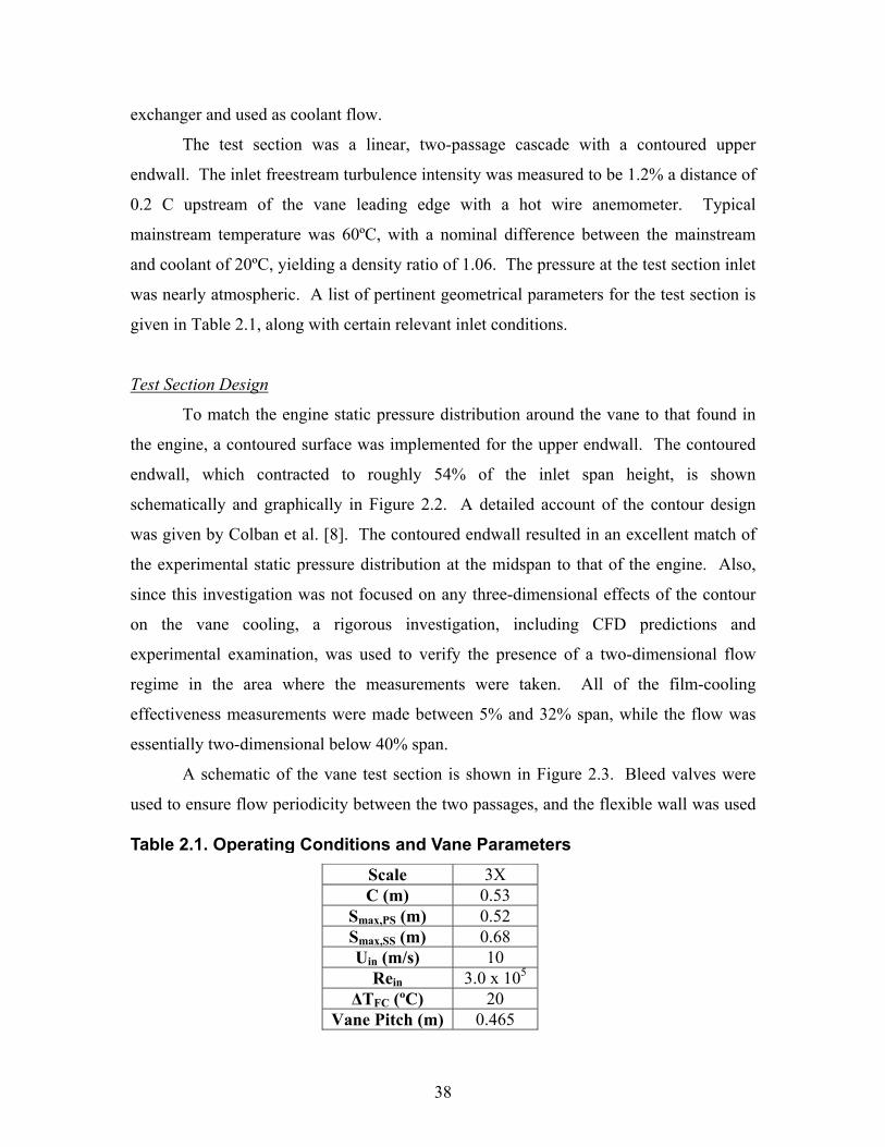
38

exchanger and used as coolant flow.

The test section was a linear, two-passage cascade with a contoured upper

endwall. The inlet freestream turbulence intensity was measured to be 1.2% a distance of

0.2 C upstream of the vane leading edge with a hot wire anemometer. Typical

mainstream temperature was 60ºC, with a nominal difference between the mainstream

and coolant of 20ºC, yielding a density ratio of 1.06. The pressure at the test section inlet

was nearly atmospheric. A list of pertinent geometrical parameters for the test section is

given in Table 2.1, along with certain relevant inlet conditions.

Test Section Design

To match the engine static pressure distribution around the vane to that found in

the engine, a contoured surface was implemented for the upper endwall. The contoured

endwall, which contracted to roughly 54% of the inlet span height, is shown

schematically and graphically in Figure 2.2. A detailed account of the contour design

was given by Colban et al. [8]. The contoured endwall resulted in an excellent match of

the experimental static pressure distribution at the midspan to that of the engine. Also,

since this investigation was not focused on any three-dimensional effects of the contour

on the vane cooling, a rigorous investigation, including CFD predictions and

experimental examination, was used to verify the presence of a two-dimensional flow

regime in the area where the measurements were taken. All of the film-cooling

effectiveness measurements were made between 5% and 32% span, while the flow was

essentially two-dimensional below 40% span.

A schematic of the vane test section is shown in Figure 2.3. Bleed valves were

used to ensure flow periodicity between the two passages, and the flexible wall was used

Scale 3X C (m) 0.53

Smax,PS (m) 0.52 Smax,SS (m) 0.68 Uin (m/s) 10

Rein 3.0 x 105 ∆TFC (ºC) 20

Vane Pitch (m) 0.465


39

0.0

0.2

0.4

0.6

0.8

1.0

-1.0 -0.5 0.0 0.5 1.0S/S

max

Z/Zmax

Pressure Side Suction Side

-SZ

+S

to make minor adjustments to the flow distribution around the center vane. Also shown

in Figure 2.3 are the plenum locations relative to the holes, as well as the hole

designations, to be used throughout the rest of the report.

A detailed discussion of the vane design and construction was given by Colban et

al. [8]. The vane contained four interior plenums, which allowed for flow rate control

amongst the rows of holes to obtain the desired blowing ratio distribution. Coolant was

PA

Flex Wall

Bleed Valve Bleed

Valve

Bypass Air

Bypass Air

PB

PC

PDSA

SC

SB

SD

Figure 2.3. Schematic of experimental test section.

Figure 2.2. Contoured endwall surface definition.

40

supplied to the plenums from the upper channel in the wind tunnel using the blower

shown in Figure 2.1. Discharge coefficients, which were presented in the study of

Colban et al. [8], were used to set the combined flow rates through each plenum based on

the desired blowing ratios.

The test vane contained showerhead cooling with five in-line rows, four fan-

shaped pressure side rows, and four fan-shaped suction side rows of film-cooling holes.

The diameter of the cylindrical inlet section of the fan-shaped holes was 0.38 ± 0.015 cm.

The diameters of each hole were measured to verify that the correct flow area was used to

determine the total mass flow rate and individual blowing ratios because of slight

manufacturing variation resulting from the five-axis water-jet machining process. Slight

variations did occur in fan-shape of the holes as a result of the manufacturing process.

Some hole-to-hole variation can be seen in the effectiveness contours, which were

attributed to variation in hole shape as well as experimental uncertainty. An illustration

of the fan-shaped hole geometry is shown in Figure 2.4, and relevant parameters for the

film-cooling holes are listed in Table 2.2. The cylindrical showerhead holes had fairly

high surface inclination angle of 60° along with a 90° compound angle. The fan-shaped

holes had a surface inclination angle of 30° and lateral and forward expansion angles of

10°.

High resolution surface temperature measurements were obtained with an IR

camera. Thermocouples placed in the vane surface were used to calibrate the images,

D

α

φ2

φ1 t

Figure 2.4. Fan shaped cooling hole detailed geometry.

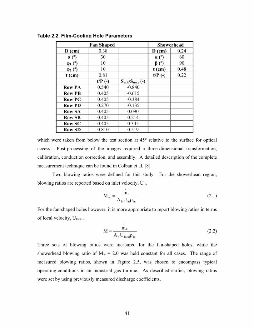
41

Fan Shaped Showerhead D (cm) 0.38 D (cm) 0.24 α (º) 30 α (º) 60 φ1 (º) 10 β (º) 90 φ2 (º) 10 t (cm) 0.48 t (cm) 0.81 t/P (-) 0.22

t/P (-) Sexit/Smax (-) Row PA 0.540 -0.840 Row PB 0.405 -0.615 Row PC 0.405 -0.384 Row PD 0.270 -0.135 Row SA 0.405 0.090 Row SB 0.405 0.214 Row SC 0.405 0.345 Row SD 0.810 0.519

which were taken from below the test section at 45° relative to the surface for optical

access. Post-processing of the images required a three-dimensional transformation,

calibration, conduction correction, and assembly. A detailed description of the complete

measurement technique can be found in Colban et al. [8].

Two blowing ratios were defined for this study. For the showerhead region,

blowing ratios are reported based on inlet velocity, Uin,

ininh

c

.

UAmM

ρ=∞ (2.1)

For the fan-shaped holes however, it is more appropriate to report blowing ratios in terms

of local velocity, Ulocal,

inlocalh

c

.

UAmM

ρ= (2.2)

Three sets of blowing ratios were measured for the fan-shaped holes, while the

showerhead blowing ratio of M∞ = 2.0 was held constant for all cases. The range of

measured blowing ratios, shown in Figure 2.5, was chosen to encompass typical

operating conditions in an industrial gas turbine. As described earlier, blowing ratios

were set by using previously measured discharge coefficients.


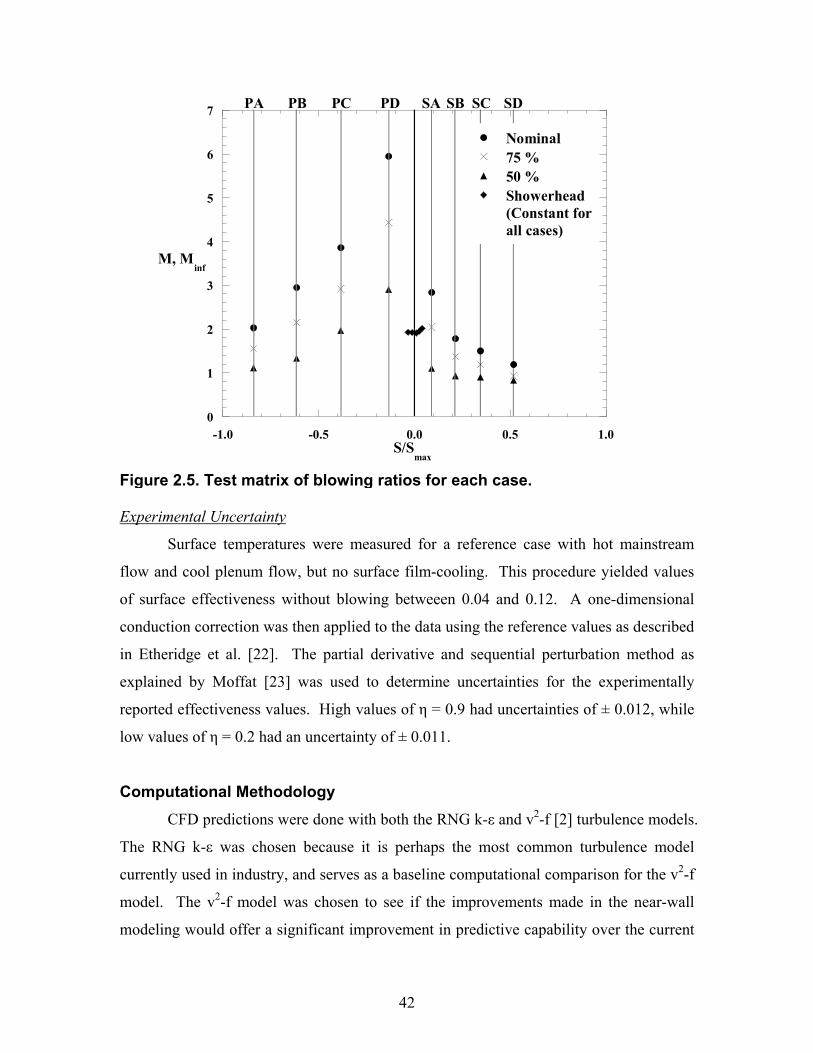
42

0

1

2

3

4

5

6

7

-1.0 -0.5 0.0 0.5 1.0

Nominal75 %50 %Showerhead(Constant forall cases)

M, Minf

S/Smax

PA PB PC PD SA SB SC SD


Surface temperatures were measured for a reference case with hot mainstream

flow and cool plenum flow, but no surface film-cooling. This procedure yielded values

of surface effectiveness without blowing betweeen 0.04 and 0.12. A one-dimensional

conduction correction was then applied to the data using the reference values as described

in Etheridge et al. [22]. The partial derivative and sequential perturbation method as

explained by Moffat [23] was used to determine uncertainties for the experimentally

reported effectiveness values. High values of η = 0.9 had uncertainties of ± 0.012, while

low values of η = 0.2 had an uncertainty of ± 0.011.

Computational Methodology CFD predictions were done with both the RNG k-ε and v2-f [2] turbulence models.

The RNG k-ε was chosen because it is perhaps the most common turbulence model

currently used in industry, and serves as a baseline computational comparison for the v2-f

model. The v2-f model was chosen to see if the improvements made in the near-wall

modeling would offer a significant improvement in predictive capability over the current

Figure 2.5. Test matrix of blowing ratios for each case.

43

industry standard. The constraints of the two models dictated different approaches in

selecting the computational domain and in meshing. All of the CFD predictions were

done using Fluent 6.0.1, a commercially available CFD solver with a special module for

the v2-f model.

RNG k-ε Model

The computational domain for the RNG k-ε simulation consisted of one periodic

vane passage. A two-dimensional view of the domain is shown in Figure 2.6. The

domain began one chord length upstream of the vane leading edge, using a velocity inlet

condition. The exit boundary was located 1.5 C downstream of the trailing edge, a

1.0 C

1.5 C

1 Pitch

Velocity Inlet

Periodic

Mass Flow Inlet

Figure 2.6. 2D view of the CFD domain (the RNG k-ε model featured the entire span and contour, while the v2-f prediction featured only a 6 cm spanwise periodic section).

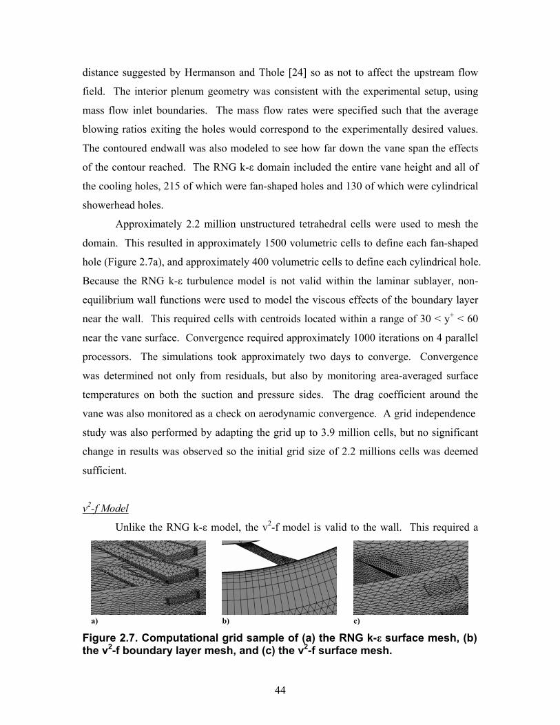
44

distance suggested by Hermanson and Thole [24] so as not to affect the upstream flow

field. The interior plenum geometry was consistent with the experimental setup, using

mass flow inlet boundaries. The mass flow rates were specified such that the average

blowing ratios exiting the holes would correspond to the experimentally desired values.

The contoured endwall was also modeled to see how far down the vane span the effects

of the contour reached. The RNG k-ε domain included the entire vane height and all of

the cooling holes, 215 of which were fan-shaped holes and 130 of which were cylindrical

showerhead holes.

Approximately 2.2 million unstructured tetrahedral cells were used to mesh the

domain. This resulted in approximately 1500 volumetric cells to define each fan-shaped

hole (Figure 2.7a), and approximately 400 volumetric cells to define each cylindrical hole.

Because the RNG k-ε turbulence model is not valid within the laminar sublayer, non-

equilibrium wall functions were used to model the viscous effects of the boundary layer

near the wall. This required cells with centroids located within a range of 30 < y+ < 60

near the vane surface. Convergence required approximately 1000 iterations on 4 parallel

processors. The simulations took approximately two days to converge. Convergence

was determined not only from residuals, but also by monitoring area-averaged surface

temperatures on both the suction and pressure sides. The drag coefficient around the

vane was also monitored as a check on aerodynamic convergence. A grid independence

study was also performed by adapting the grid up to 3.9 million cells, but no significant

change in results was observed so the initial grid size of 2.2 millions cells was deemed

sufficient.

v2-f Model

Unlike the RNG k-ε model, the v2-f model is valid to the wall. This required a

a) b) c)

Figure 2.7. Computational grid sample of (a) the RNG k-ε surface mesh, (b) the v2-f boundary layer mesh, and (c) the v2-f surface mesh.

45

structured grid in the vicinity of the wall, resolving the boundary layer to within y+ < 3.

Consequently, modeling the entire span was not a possibility for the v2-f model due to the

higher cell density required near the wall. For this reason, only a 6 cm spanwise periodic

section was included in the computational domain, which is shown schematically in

Figure 2.6. Both the experimental results and the RNG k-ε CFD results showed

periodicity below the midspan, so it was valid to model only the small periodic section,

thus making the computations feasible.

The v2-f model grid contained approximately 1.6 million cells in order to get the

near wall resolution. The vane surface was meshed with an unstructured grid, and a

boundary layer mesh was applied to the vane surface (shown in Figure 2.7b).

Consequently, there were prismatic cells to a distance of 1.5 cm from the wall, at which

point the remainder of the domain was meshed with unstructured tetrahedral cells. The

surface mesh resolution is shown for the v2-f simulations in Figure 2.7c. Solutions were

run for 500 iterations on a first order upwind scheme, before being switched over to a

second order upwind scheme with SIMPLEC coupling for 1500 iterations. The v2-f

model computations were run on 3 parallel processors and required approximately 3 days

to reach convergence. As with the RNG k-ε model, the surface temperatures and drag

coefficient were monitored as additional convergence criteria.

Results Prior to performing the multiple row adiabatic film-cooling measurements, the

experimental method and data reduction procedure were validated for a single row and

compared to existing published data. Figure 2.8 shows laterally averaged single row

effectiveness downstream of row SC, a row which was located in a relatively flat region

of the vane. Because of differences in hole geometry and spacing, the distance

downstream of the hole exit was normalized with respect to the equivalent exit slot width

s, where s was the ratio of the hole breakout area to the hole spacing P. The results show

excellent agreement with the flat plate study by Gritsch et al. [25], thus validating both

the experimental and data reduction methods.

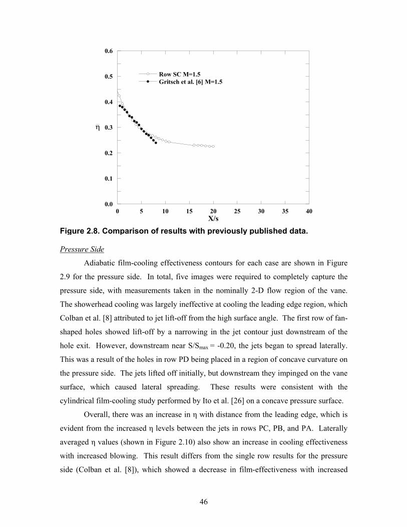
46

0.0

0.1

0.2

0.3

0.4

0.5

0.6

0 5 10 15 20 25 30 35 40

Row SC M=1.5Gritsch et al. [6] M=1.5

X/s

η

Pressure Side

Adiabatic film-cooling effectiveness contours for each case are shown in Figure

2.9 for the pressure side. In total, five images were required to completely capture the

pressure side, with measurements taken in the nominally 2-D flow region of the vane.

The showerhead cooling was largely ineffective at cooling the leading edge region, which

Colban et al. [8] attributed to jet lift-off from the high surface angle. The first row of fan-

shaped holes showed lift-off by a narrowing in the jet contour just downstream of the

hole exit. However, downstream near S/Smax = -0.20, the jets began to spread laterally.

This was a result of the holes in row PD being placed in a region of concave curvature on

the pressure side. The jets lifted off initially, but downstream they impinged on the vane

surface, which caused lateral spreading. These results were consistent with the

cylindrical film-cooling study performed by Ito et al. [26] on a concave pressure surface.

Overall, there was an increase in η with distance from the leading edge, which is

evident from the increased η levels between the jets in rows PC, PB, and PA. Laterally

averaged η values (shown in Figure 2.10) also show an increase in cooling effectiveness

with increased blowing. This result differs from the single row results for the pressure

side (Colban et al. [8]), which showed a decrease in film-effectiveness with increased

Figure 2.8. Comparison of results with previously published data.

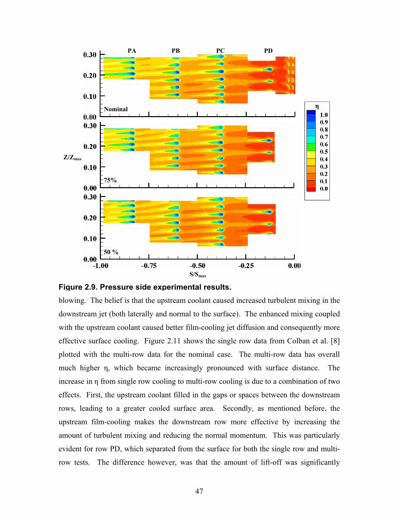
47

blowing. The belief is that the upstream coolant caused increased turbulent mixing in the

downstream jet (both laterally and normal to the surface). The enhanced mixing coupled

with the upstream coolant caused better film-cooling jet diffusion and consequently more

effective surface cooling. Figure 2.11 shows the single row data from Colban et al. [8]

plotted with the multi-row data for the nominal case. The multi-row data has overall

much higher η, which became increasingly pronounced with surface distance. The

increase in η from single row cooling to multi-row cooling is due to a combination of two

effects. First, the upstream coolant filled in the gaps or spaces between the downstream

rows, leading to a greater cooled surface area. Secondly, as mentioned before, the

upstream film-cooling makes the downstream row more effective by increasing the

amount of turbulent mixing and reducing the normal momentum. This was particularly

evident for row PD, which separated from the surface for both the single row and multi-

row tests. The difference however, was that the amount of lift-off was significantly

S/Smax

Z/Zmax

Nominal

75%

50 %

η

PA PB PC PD

Figure 2.9. Pressure side experimental results.

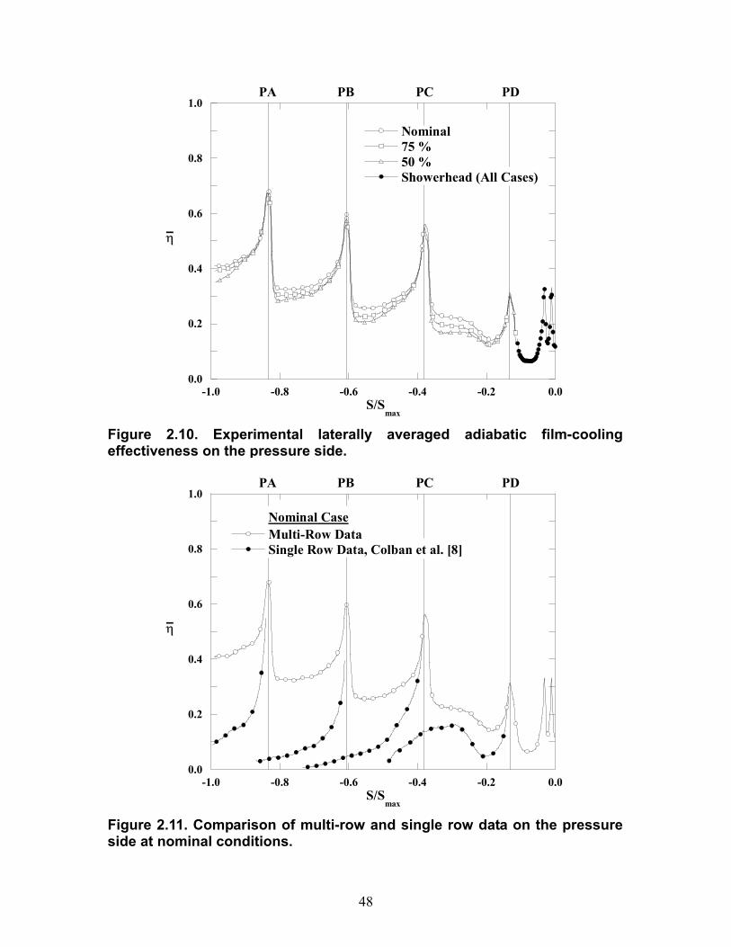
48

0.0

0.2

0.4

0.6

0.8

1.0

-1.0 -0.8 -0.6 -0.4 -0.2 0.0

Nominal75 %50 %Showerhead (All Cases)

S/Smax

η

PA PB PC PD

0.0

0.2

0.4

0.6

0.8

1.0

-1.0 -0.8 -0.6 -0.4 -0.2 0.0

Multi-Row DataSingle Row Data, Colban et al. [8]

S/Smax

η

PA PB PC PD

Nominal Case

Figure 2.10. Experimental laterally averaged adiabatic film-cooling effectiveness on the pressure side.

Figure 2.11. Comparison of multi-row and single row data on the pressure side at nominal conditions.

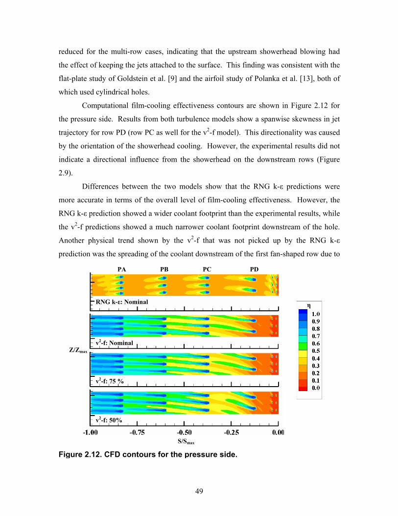
49

reduced for the multi-row cases, indicating that the upstream showerhead blowing had

the effect of keeping the jets attached to the surface. This finding was consistent with the

flat-plate study of Goldstein et al. [9] and the airfoil study of Polanka et al. [13], both of

which used cylindrical holes.

Computational film-cooling effectiveness contours are shown in Figure 2.12 for

the pressure side. Results from both turbulence models show a spanwise skewness in jet

trajectory for row PD (row PC as well for the v2-f model). This directionality was caused

by the orientation of the showerhead cooling. However, the experimental results did not

indicate a directional influence from the showerhead on the downstream rows (Figure

2.9).

Differences between the two models show that the RNG k-ε predictions were

more accurate in terms of the overall level of film-cooling effectiveness. However, the

RNG k-ε prediction showed a wider coolant footprint than the experimental results, while

the v2-f predictions showed a much narrower coolant footprint downstream of the hole.

Another physical trend shown by the v2-f that was not picked up by the RNG k-ε

prediction was the spreading of the coolant downstream of the first fan-shaped row due to

RNG k-ε: Nominal

v2-f: Nominal

v2-f: 75 %

v2-f: 50%

η

PA PB PC PD

S/Smax

Z/Zmax

Figure 2.12. CFD contours for the pressure side.

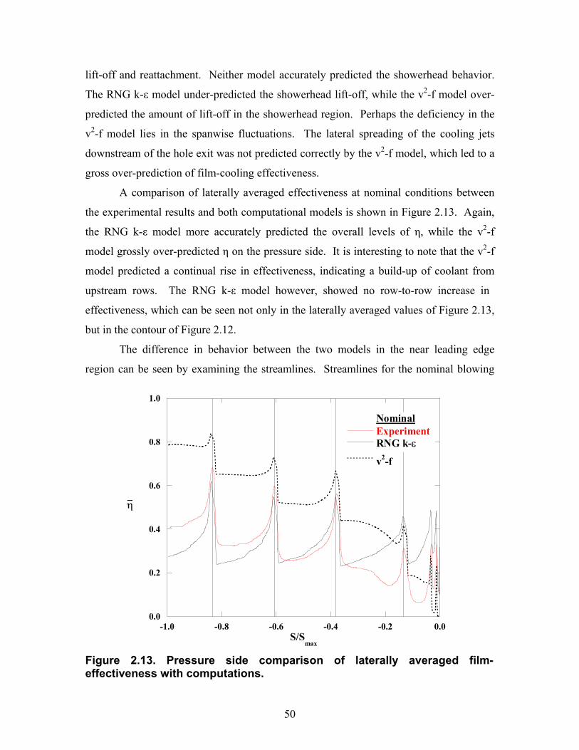
50

lift-off and reattachment. Neither model accurately predicted the showerhead behavior.

The RNG k-ε model under-predicted the showerhead lift-off, while the v2-f model over-

predicted the amount of lift-off in the showerhead region. Perhaps the deficiency in the

v2-f model lies in the spanwise fluctuations. The lateral spreading of the cooling jets

downstream of the hole exit was not predicted correctly by the v2-f model, which led to a

gross over-prediction of film-cooling effectiveness.

A comparison of laterally averaged effectiveness at nominal conditions between

the experimental results and both computational models is shown in Figure 2.13. Again,

the RNG k-ε model more accurately predicted the overall levels of η, while the v2-f

model grossly over-predicted η on the pressure side. It is interesting to note that the v2-f

model predicted a continual rise in effectiveness, indicating a build-up of coolant from

upstream rows. The RNG k-ε model however, showed no row-to-row increase in

effectiveness, which can be seen not only in the laterally averaged values of Figure 2.13,

but in the contour of Figure 2.12.

The difference in behavior between the two models in the near leading edge

region can be seen by examining the streamlines. Streamlines for the nominal blowing

0.0

0.2

0.4

0.6

0.8

1.0

-1.0 -0.8 -0.6 -0.4 -0.2 0.0

ExperimentRNG k-ε

v2-f

S/Smax

η

Nominal

Figure 2.13. Pressure side comparison of laterally averaged film-effectiveness with computations.

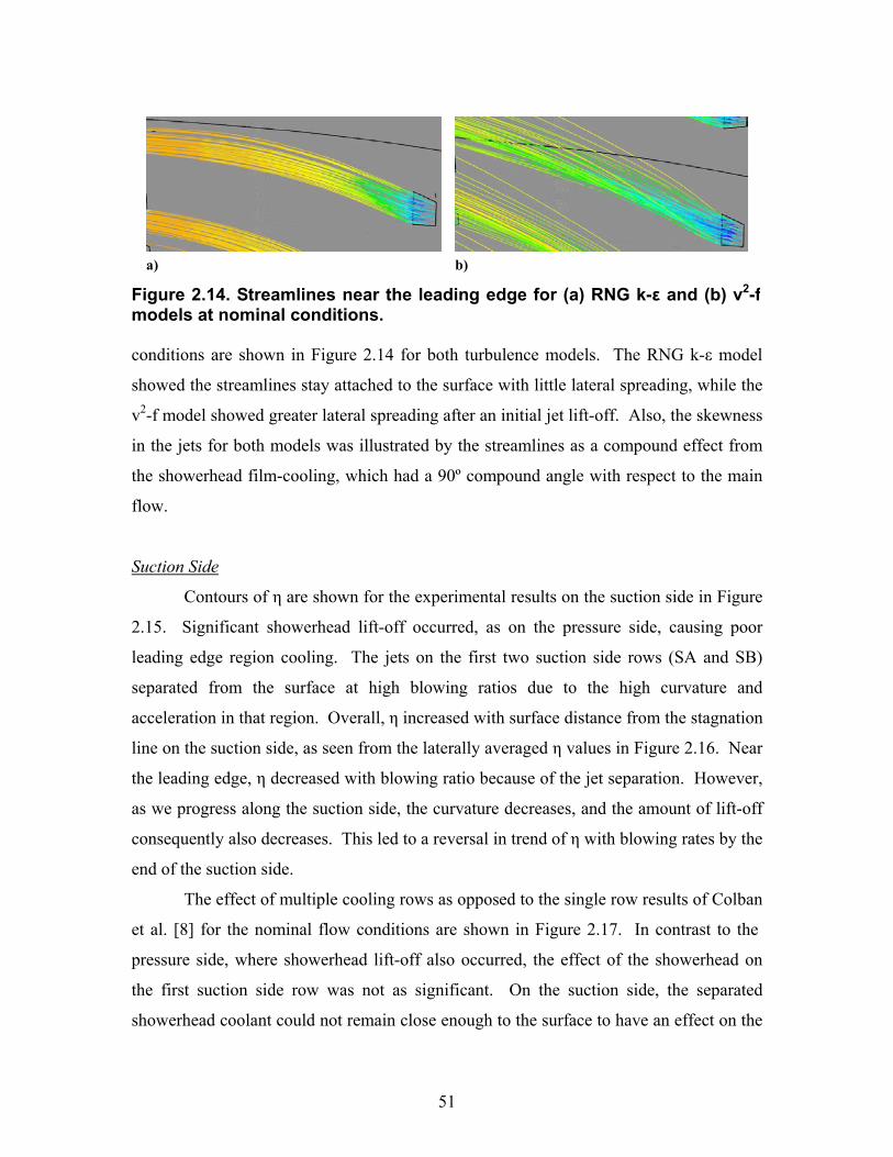
51

conditions are shown in Figure 2.14 for both turbulence models. The RNG k-ε model

showed the streamlines stay attached to the surface with little lateral spreading, while the

v2-f model showed greater lateral spreading after an initial jet lift-off. Also, the skewness

in the jets for both models was illustrated by the streamlines as a compound effect from

the showerhead film-cooling, which had a 90º compound angle with respect to the main

flow.

Suction Side

Contours of η are shown for the experimental results on the suction side in Figure

2.15. Significant showerhead lift-off occurred, as on the pressure side, causing poor

leading edge region cooling. The jets on the first two suction side rows (SA and SB)

separated from the surface at high blowing ratios due to the high curvature and

acceleration in that region. Overall, η increased with surface distance from the stagnation

line on the suction side, as seen from the laterally averaged η values in Figure 2.16. Near

the leading edge, η decreased with blowing ratio because of the jet separation. However,

as we progress along the suction side, the curvature decreases, and the amount of lift-off

consequently also decreases. This led to a reversal in trend of η with blowing rates by the

end of the suction side.

The effect of multiple cooling rows as opposed to the single row results of Colban

et al. [8] for the nominal flow conditions are shown in Figure 2.17. In contrast to the

pressure side, where showerhead lift-off also occurred, the effect of the showerhead on

the first suction side row was not as significant. On the suction side, the separated

showerhead coolant could not remain close enough to the surface to have an effect on the

Figure 2.14. Streamlines near the leading edge for (a) RNG k-ε and (b) v2-f models at nominal conditions.

a) b)

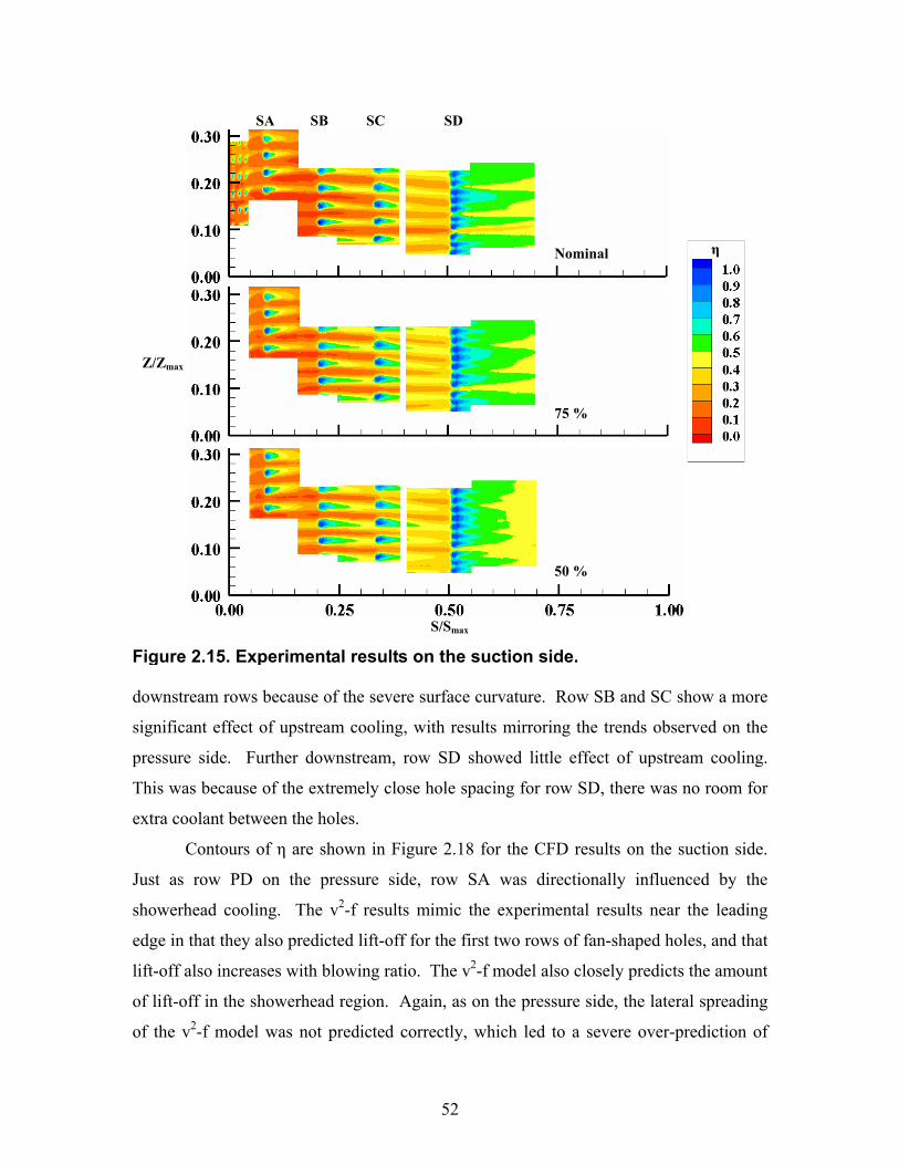
52

downstream rows because of the severe surface curvature. Row SB and SC show a more

significant effect of upstream cooling, with results mirroring the trends observed on the

pressure side. Further downstream, row SD showed little effect of upstream cooling.

This was because of the extremely close hole spacing for row SD, there was no room for

extra coolant between the holes.

Contours of η are shown in Figure 2.18 for the CFD results on the suction side.

Just as row PD on the pressure side, row SA was directionally influenced by the

showerhead cooling. The v2-f results mimic the experimental results near the leading

edge in that they also predicted lift-off for the first two rows of fan-shaped holes, and that

lift-off also increases with blowing ratio. The v2-f model also closely predicts the amount

of lift-off in the showerhead region. Again, as on the pressure side, the lateral spreading

of the v2-f model was not predicted correctly, which led to a severe over-prediction of

S/Smax

Z/Zmax

Nominal

75 %

50 %

SA SB SC SD

η

Figure 2.15. Experimental results on the suction side.

53

0.0

0.2

0.4

0.6

0.8

1.0

0.0 0.2 0.4 0.6 0.8 1.0

Nominal75 %50 %Showerhead(All Cases)

S/Smax

η

SA SB SC SD

0.0

0.2

0.4

0.6

0.8

1.0

0.0 0.2 0.4 0.6 0.8 1.0

Multi-Row DataSingle Row DataColban et al. [8]

S/Smax

η

SA SB SC SD

Nominal

Figure 2.17. Comparison of multi-row and single row data on the suction side at nominal conditions.

Figure 2.16. Experimental laterally averaged adiabatic film-cooling effectiveness on the suction side.

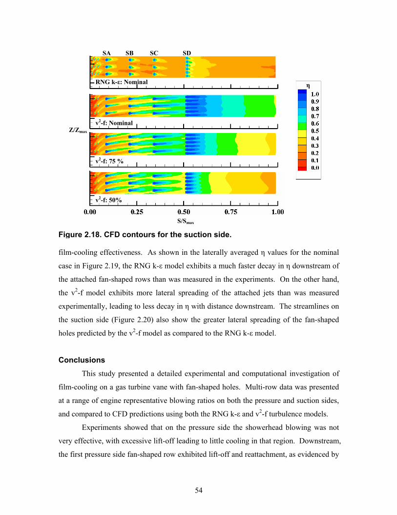
54

film-cooling effectiveness. As shown in the laterally averaged η values for the nominal

case in Figure 2.19, the RNG k-ε model exhibits a much faster decay in η downstream of

the attached fan-shaped rows than was measured in the experiments. On the other hand,

the v2-f model exhibits more lateral spreading of the attached jets than was measured

experimentally, leading to less decay in η with distance downstream. The streamlines on

the suction side (Figure 2.20) also show the greater lateral spreading of the fan-shaped

holes predicted by the v2-f model as compared to the RNG k-ε model.

Conclusions This study presented a detailed experimental and computational investigation of

film-cooling on a gas turbine vane with fan-shaped holes. Multi-row data was presented

at a range of engine representative blowing ratios on both the pressure and suction sides,

and compared to CFD predictions using both the RNG k-ε and v2-f turbulence models.

Experiments showed that on the pressure side the showerhead blowing was not

very effective, with excessive lift-off leading to little cooling in that region. Downstream,

the first pressure side fan-shaped row exhibited lift-off and reattachment, as evidenced by

Figure 2.18. CFD contours for the suction side.

η RNG k-ε: Nominal

v2-f: Nominal

v2-f: 75 %

v2-f: 50%

SA SB SC SD

S/Smax

Z/Zmax

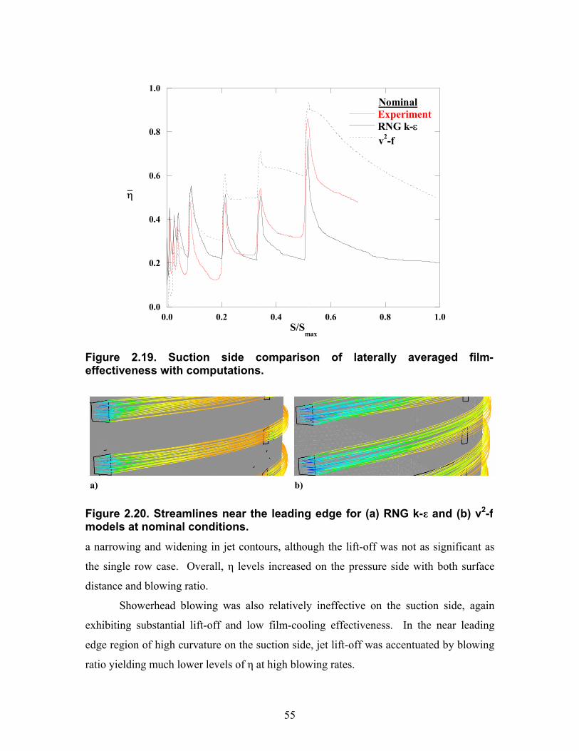
55

0.0

0.2

0.4

0.6

0.8

1.0

0.0 0.2 0.4 0.6 0.8 1.0

ExperimentRNG k-εv2-f

S/Smax

η

Nominal

a narrowing and widening in jet contours, although the lift-off was not as significant as

the single row case. Overall, η levels increased on the pressure side with both surface

distance and blowing ratio.

Showerhead blowing was also relatively ineffective on the suction side, again

exhibiting substantial lift-off and low film-cooling effectiveness. In the near leading

edge region of high curvature on the suction side, jet lift-off was accentuated by blowing

ratio yielding much lower levels of η at high blowing rates.

Figure 2.20. Streamlines near the leading edge for (a) RNG k-ε and (b) v2-f models at nominal conditions.

a) b)

Figure 2.19. Suction side comparison of laterally averaged film-effectiveness with computations.

56

The CFD predictions did not agree well with the experimental results for the most

part, at best capturing either the correct η levels or some of the correct physics, but not

both. The v2-f model more nearly predicted the actual flow physics in terms of

separation, however it had difficulty in accurately predicting the lateral spreading

correctly leading of over-predictions of film-cooling effectiveness. The RNG k-ε model,

on the other hand, offered a better match with the experimental data in terms of correct

effectiveness levels. Although there have been matching CFD predictions for flat plate

film-cooling, clearly more advances in CFD turbulence modeling are required before the

highly complex flow of film-cooling on a gas turbine vane can be modeled accurately.

Acknowledgments The authors are grateful to Siemens Power Generation for their funding and


Nomenclature A area

C vane true chord

CD discharge coefficient


f elliptic relaxation function

k turbulent kinetic energy

kcond thermal conductivity

.m mass flow rate

M blowing ratio using local velocity, M = mc/AhUlocalρin

M∞ blowing ratio using inlet velocity, M∞ = mc/AhUinρin

P hole spacing measured normal to streamwise direction

P vane pitch

Re Reynolds number, Re = UinC/ν

s equivalent slot width, s = Abreak/P

S distance along the vane surface


57

T temperature

U velocity

v2 normal velocity fluctuations

X distance downstream of the hole exit

y+ wall coordinate

Z distance measured along the vane span

Greek


β compound angle

ε eddy viscosity, surface emmissivity

µt turbulent viscosity

ν kinematic viscosity

η adiabatic film-cooling effectiveness, η = (T∞ – Tad)/(T∞ – Tc)

ρ density



Subscripts

ad adiabatic

break hole breakout area

c coolant

exit hole exit

h metering area of film-cooling holes based on D

in inlet condition

local local conditions

max maximum

plenumplenum conditions

surf surface

∞ freestream conditions

58

References [1] R. J. Goldstein, E. R. G. Eckert, and F. Burggraf, "Effects of Hole Geometry and

Density on Three-Dimensional Film Cooling," ASME Journal of Heat and Mass

Transfer, vol. 17, pp. 595-607, 1974.

[2] P. A. Durbin, "Near-Wall Turbulence Closure Modeling Without 'Damping

Functions'," Theoretical and Computational Fluid Dynamics, vol. 3, pp. 1-13,

1991.

[3] D. M. Kercher, Film-Cooling Bibliography: 1940-2002: Private publication, 2003.

[4] D. M. Kercher, Film-Cooling Bibliography Addendum: 1999-2004: Private

publication, 2005.

[5] R. S. Bunker, "A Review of Shaped Hole Turbine Film-Cooling Technology,"

ASME Journal of Heat Transfer, vol. 127, pp. 441-453, 2005.

[6] L. Zhang, M. Baltz, R. Pudupatty, and M. Fox, "Turbine Nozzle Film-Cooling

Study Using the Pressure Sensitive Paint (PSP) Technique," 99-GT-196, 1999.

[7] L. Zhang and R. Pudupatty, "The Effects of Injection Angle and Hole Exit Shape

on Turbine Nozzle Pressure Side Film-cooling," 2000-GT-247, 2000.

[8] W. Colban, A. Gratton, K. A. Thole, and M. Haendler, "Heat Transfer and Film-

Cooling Measurements on a Stator Vane with Fan-Shaped Cooling Holes,"

GT2005-68258, 2005.

[9] R. J. Goldstein, E. R. G. Eckert, H. D. Chiang, and E. Elovic, "Effect of Surface

Roughness on Film Cooling Performance," ASME Journal of Engineering for Gas

Turbines and Power, vol. 107, pp. 111-116, 1985.

59

[10] S. M. Guo, C. C. Lai, T. V. Jones, M. L. G. Oldfield, G. D. Lock, and A. J.

Rawlinson, "The Application of Thin-Film Technology to Measure Turbine-Vane

Heat Transfer and Effectiveness in a Film-Cooled, Engine-Simulated

Environment," International Journal of Heat and Fluid Flow, vol. 19, pp. 594-600,

1998.

[11] J. E. Sargison, S. M. Guo, M. L. G. Oldfield, G. D. Lock, and A. J. Rawlinson, "A

Converging Slot-Hole Film-Cooling Geometry Part 2: Transonic Nozzle Guide

Vane Heat Transfer and Loss," 2001-GT-0127, 2001.

[12] M. Schnieder, S. Parneix, and J. von Wolfersdorf, "Effect of Showerhead

Injection on Superposition of Multi-Row Pressure Side Film-Cooling with Fan

Shaped Holes," GT2003-38693, 2003.

[13] M. D. Polanka, M. I. Ethridge, J. M. Cutbirth, and D. G. Bogard, "Effects of

Showerhead Injection on Film Cooling Effectiveness for a Downstream Row of

Holes," 2000-GT-240, 2000.

[14] H. Riess and A. Bölcs, "The Influence of the Boundary Layer State and Reynolds

Number on Film-cooling and Heat Transfer on a Cooled Nozzle Guide Vane,"

2000-GT-205, 2000.

[15] A. Kohli and K. A. Thole, "A CFD Investigation on the Effects of Entrance

Crossflow Directions to Film-Cooling Holes," 32nd National Heat Transfer

Conference, vol. 12, pp. 223-232, 1997.

[16] D. G. Hyams and J. H. Leylek, "A Detailed Analysis of Film Cooling Physics Part

III: Streamwise Injection with Shaped Holes," 97-GT-271, 1997.

[17] T. Hildebrandt, W. Ganzert, and L. Fottner, "Systematic Experimental and

Numerical Investigations on the Aerothermodynamics of a Film Cooled Turbine

60

Cascade with Variation of the Cooling Hole Shape Part II: Numerical Approach,"

2000-GT-298, 2000.

[18] J. D. Ferguson, J. H. Leylek, and F. A. Buck, "Film Cooling on a Modern HP

Turbine Blade Part III: Axial Shaped Holes," GT-2002-30522, 2002.

[19] J. D. Heidmann, A. J. Kassab, E. A. Divo, F. Rodriguez, and E. Steinthorsson,

"Conjugate Heat Transfer Effects on a Realistic Film-Cooled Turbine Vane,"

GT2003-38553, 2003.

[20] S. Parneix, P. A. Durbin, and M. Behnia, "Computation of 3-D Turbulent

Boundary Layers Using the V2F Model," Flow, Turbulence, and Combustion, vol.

60, pp. 19-46, 1998.

[21] P. A. Durbin, "Separated Flow Computations with the k-e-v2 Model," AIAA

Journal, vol. 33, pp. 659-664, 1995.

[22] M. I. Ethridge, J. M. Cutbirth, and D. G. Bogard, "Scaling of Performance for

Varying Density Ratio Coolants on an Airfoil with Strong Curvature and Pressure

Gradient Effects," 2000-GT-239, 2000.

[23] R. J. Moffat, "Describing the Uncertainties in Experimental Results,"

Experimental Thermal and Fluid Science, vol. 1, pp. 3-17, 1988.

[24] K. S. Hermanson and K. A. Thole, "Effect of Inlet Conditions on Endwall

Secondary Flows," Journal of Propulsion and Power, vol. 16, pp. 286-296, 2000.

[25] M. Gritsch, A. Schulz, and S. Wittig, "Adiabatic Wall Effectiveness

Measurements of Film-Cooling Holes With Expanded Exits," ASME Journal of

Turbomachinery, vol. 120, pp. 549-556, 1998.

61

[26] S. Ito, R. J. Goldstein, and E. R. G. Eckert, "Film Cooling of a Gas Turbine

Blade," Journal of Engineering for Power, vol. 100, pp. 476-481, 1978.




Submitted to the 2006 ASME Turbo Expo*

Abstract Fan-shaped film-cooling holes have been shown to provide superior cooling

performance to cylindrical holes along flat-plates and turbine airfoils over a large range

of different conditions. Benefits of fan-shaped holes include less required cooling air for

the same performance, increased part lifetime, and fewer required holes. The major

drawback however, is increased manufacturing cost and manufacturing difficulty,

particularly for the vane platform region.

To this point, there have only been extremely limited comparisons between

cylindrical and shaped holes on a turbine endwall at either low or high freestream

turbulence conditions. This study presents film-cooling effectiveness measurements on

an endwall surface in a large-scale, low-speed, two-passage, linear vane cascade. Results

showed that film-cooling effectiveness decreased with increasing blowing rate for the

cylindrical holes, indicating jet lift-off. However, the fan-shaped passage showed

increased film-cooling effectiveness with increasing blowing ratio. Overall, fan-shaped

holes increased film-cooling effectiveness by an average of 75% over cylindrical holes.

63

Introduction The primary goal of turbine cooling research during the past years was to develop

cooling methods in which the amount of coolant could be decreased with at least the

same, if not better, cooling performance. Fan-shaped holes have provided this

opportunity to engine designers by providing significantly better cooling performance

compared to cylindrical holes over a large range in blowing ratios and other conditions.

However, the main drawback in implementing fan-shaped holes into current engine

designs comes from the manufacturing side. Fan-shaped holes are on the order of four to

eight times more expensive to manufacture than cylindrical holes on a per hole basis,

depending on the technique. Fan-shaped holes are generally made using the electro-

discharge machining technique, which is much more expensive than the cheaper laser-

drilling methods typically used to manufacture cylindrical holes.

The benefits of shaped hole cooling over cylindrical hole cooling for flat-plates

and airfoils were reviewed by Bunker [1]. Lateral expansion of the coolant promotes a

better coverage of surface area downstream of the hole. Exit momentum of the jet is

reduced as a result of the hole expansion, which keeps the jet attached to the surface.

Both of these benefits were illustrated by the flow visualization study of Goldstein et al.

[2].

Although shaped cooling holes have been widely used on the airfoil surface,

manufacturing difficulties have limited their use on the vane platform region. For this

reason, the majority of endwall cooling studies have used cylindrical cooling holes.

However, recent advances in manufacturing coupled with the desire for more efficient

cooling, have allowed shaped holes to be used in the platform region. Unlike the

majority of the airfoil surface, the endwall is a highly three-dimensional region, with

intense secondary flows caused by the approaching boundary layer and cross-passage

pressure gradient. This inevitably makes endwall film-cooling more challenging to

design and to predict.

This study was spawned from the lack of research of shaped hole endwall film-

cooling. It was necessary to directly compare the performance of shaped to cylindrical

cooling holes, since cylindrical holes provide most of the current research. This study

contained two separate vane passages, one with cylindrical endwall film-cooling holes,

64

and the other with shaped endwall film-cooling holes. A double row of staggered

cylindrical film-cooling holes was located upstream of both passages. Comparisons were

directly made based on matching coolant mass flow rates between the two passages. The

effect of freestream turbulence was also investigated because today’s gas turbines can

have a range of different freestream turbulence levels exiting the combustor.

Past Studies

Film-cooling has been studied at great length over the past 50 years (Kercher [3],

[4]). Excellent reviews of film-cooling research can be found in Goldstein [5], Bogard

and Thole [6], and for shaped film-cooling holes by Bunker [1]. A fair amount of

endwall film-cooling research has been done using slots and discrete cylindrical holes,

however, only the studies by Vogel et al. [7], Vogel [8], and Barrigozzi [9] have

employed shaped holes.

One of the main influences on endwall film-cooling is the passage vortex and

subsequent cross passage flow. This tends to sweep the coolant away from the pressure

side towards the suction side. This effect has been shown for upstream slot cooling by

Blair [10], Granser and Schulenberg [11], Colban et al. [12], and Knost and Thole [13]

and for cylindrical film-cooling holes by Harasgama and Burton [14] and Nicklas [15].

Not only does the endwall secondary flow affect the film-cooling, but the film-

cooling also has an effect on the secondary flow field. Increased film-cooling has been

shown to reduce the strength of the passage vortex, as well as reduce the amount of cross

passage flow. This effect has been shown by Sieverding and Wilputte [16] and Kost and

Nicklas [17] for endwall cooling injection and Colban et al. [18] for upstream slot

injection from a backward-facing step.

Friedrichs et al. [19] studied cylindrical endwall cooling in a rig specially

designed to generate stronger secondary flows in order to isolate the effect of the

secondary flow field on endwall cooling. They identified barriers to the endwall coolant

flow in the form of three-dimensional separation lines on the endwall formed by the

secondary flow structures. Coolant ejected near these separation lines was swept off the

endwall surface, providing little cooling benefit. However, cooling ejection farther from

the secondary flow separation lines provided better cooling. They also reported that the

65

addition of film-cooling had an effect on the near wall secondary flow structures,

redirecting the cross passage flow in the direction of the inviscid streamlines. Friedrichs

et al. [19] also found that the coolant trajectories were in large part dictated by the

direction of the near wall flow, not the ejection angle of the hole. The insensitivity of the

jet trajectory to the hole orientation angle has also been verified by Knost and Thole [20].

Studies of double rows of staggered cylindrical holes upstream of the leading

edge have been performed by Oke et al. [21], Zhang and Jaiswal [22], and Zhang and

Moon [23]. Oke et al. [21] measured thermal and velocity profiles in the vane passage

downstream of 45º holes. Their results showed jet lift-off just downstream of the holes,

which resulted in high mixing of the jets with the freestream. Both Zhang and Jaiswal

[22] (using 45º holes) and Zhang and Moon [23] (using 30º holes) showed that at low

flow rates the majority of the coolant was swept away from the pressure side towards the

suction side because of the cross passage flow. However, they found that at higher flow

rates, the coolant ejection suppressed the endwall secondary flow, leading to both thermal

and aerodynamic benefits.

To date, only the studies by Vogel et al. [7], Vogel [8], and Barigozzi et al. [9]

have featured shaped hole film-cooling on the endwall. The first two studies were

primarily focused on the development of a unique experimental technique. However, a

number of conclusions can be made about the behavior of shaped cooling holes on an

endwall from the images presented in that work. The lateral spreading of coolant

typically seen on flat-plate and airfoil surfaces with fan-shaped film-cooling also

occurred on the endwall. The coolant was still largely affected by the cross-passage flow,

and was directed away from the pressure side towards the suction side. Also, jets that

were located directly downstream of other coolant trajectories tended to provide the best

film-effectiveness.

Barigozzi et al. [9] measured film-effectiveness, total pressure loss, flow field,

and thermal field data for an endwall cooled with cylindrical holes and conical diffuser

shaped holes. However, their comparison between cylindrical and conical shaped holes

was not exact, since there were different hole patterns. Barigozzi et al. [9] showed that

the size and vorticity of the passage vortex actually increased with decreasing film-

cooling mass flow rates. As the flow rate increased above 1%, the passage vortex

66

diminished in size and strength until it was no longer recognizable. The endwall cross

flow was also eliminated at the highest mass flow rate (MFR), resulting in a nearly

uniform two-dimensional exit flow. This result was confirmed with the film-

effectiveness measurements, which showed that at low flow rates the jets were deflected

towards the suction side, while at high flow rates the jets followed the potential flow

streamlines. At low flow rates the cylindrical holes performed slightly better than the

conical shaped holes, because the lower momentum jets exiting the shaped holes were

more affected by the secondary flows. However, at higher flow rates, the conical shaped

holes provided much better cooling than the cylindrical holes, in part because of the

increased coverage and reduced exit momentum.

Experimental Facilities

The experiments were performed in the Virginia Tech Experimental and

Computational Convection Laboratory low-speed, large-scale, recirculating wind tunnel

facility shown in Figure 3.1. The wind tunnel featured a flow split section, which divided

the flow into three separate channels. The air in the center channel was heated by a 55

kW heater bank to simulate the combustor core flow, and then passed through a series of

flow straighteners before entering the test section. The air in the two outer channels was

cooled using heat exchangers supplied by a 44 kW chiller, and then used as supply

coolant. The coolant was delivered to the endwall plenum by a 2 hp blower situated atop

the wind tunnel. This process resulted in temperature differences between the coolant


Fan


HeaterCoolers

Screens


Section


Section


Vane Cascade


67

and mainstream of approximately 20ºC.

The Reynolds number based on true vane chord and inlet velocity was 3.4x105 for

all tests. Profiles of temperature and velocity were made upstream of each passage prior

to testing to ensure periodicity amongst both passages. The tests were essentially

incompressible, with a jet-to-freestream density ratio of approximately 1.06. The inlet

turbulence intensity was measured at a location of X/C = -0.3 upstream of the test section

with a hot wire anemometer. Turbulence intensity for the low freestream conditions was

measured to be 1.2%. High freestream turbulence was generated using three 7.2 cm

diameter normal jets in crossflow, which were located 2.7 chord lengths upstream of the

vane leading edge. This resulted in 8.9% turbulence intensity with a length scale of Λx/P

= 0.15. The approaching boundary layer thickness was also measured to be δ/Zmax = 0.12

at a distance X/C = -0.3 upstream of the vane leading edge. A summary of important

inlet conditions and geometrical parameters is given in Table 3.1.

Test Section Design

The two-passage linear vane cascade test section described in detail by Colban et

al. [24] was used. A contoured upper endwall was designed to ensure the engine static

pressure distribution around the vane surface was matched. It was critical to match the

static pressure distribution around the vane surface, as the location of minimum static

pressure has a significant effect on the development of the passage secondary flows. The

pressure coefficient distributions around the vane at engine conditions and in the low

speed facility both with and without the contour are shown in Figure 3.2. The contoured

vane was aft-loaded, which leads to weaker secondary flows since the minimum driving

pressure is further from the leading edge. Without the contoured endwall, the vane was

Scale 3X C (m) 0.53

Smax,PS (m) 0.52 Smax,SS (m) 0.68 Uin (m/s) 10 Rein (-) 3.4 x 105

∆TFC (ºC) 20 Vane Pitch (m) 0.465


68

-40

-35

-30

-25

-20

-15

-10

-5

0

-1.0 -0.5 0.0 0.5 1.0

Enginew/o Contourw/ContourExperimental

Cp

S/Smax

fore

aft

more fore-loaded, which tends to strengthen the secondary flow structures because of a

larger driving pressure difference in the passage. Clearly with the contoured endwall, the

pressure distribution around the vane was very similar to the engine conditions, which led

to closely simulated engine representative secondary flows in the vane cascade.

Some modifications to the previously described [24] test section were made. A

film-cooled endwall surface was placed on the lower flat platform, and a feed plenum

was constructed below. The inner passage of the cascade featured cylindrical holes,

while the outer passage featured fan-shaped holes. Figure 3.3 shows the hole layout on

the endwall, including the two rows of staggered cylindrical holes that were placed

upstream of each passage. The layout of the film-cooling holes was identical for each

passage, which allowed a direct comparison of the respective cooling performance of

each hole geometry.

The endwall was constructed from medium density foam with a low thermal

conductivity (k = 0.028 W/m·K) to allow adiabatic film-cooling effectiveness

measurements and it was manufactured using a five-axis water jet cutting machine. The

relevant geometrical parameters of the film-cooling holes are summarized in Table 3.2.

All of the holes had a cylindrical diameter of 0.26 ± 0.015 cm. The two upstream rows of

Figure 3.2. Static pressure distribution around the center vane.

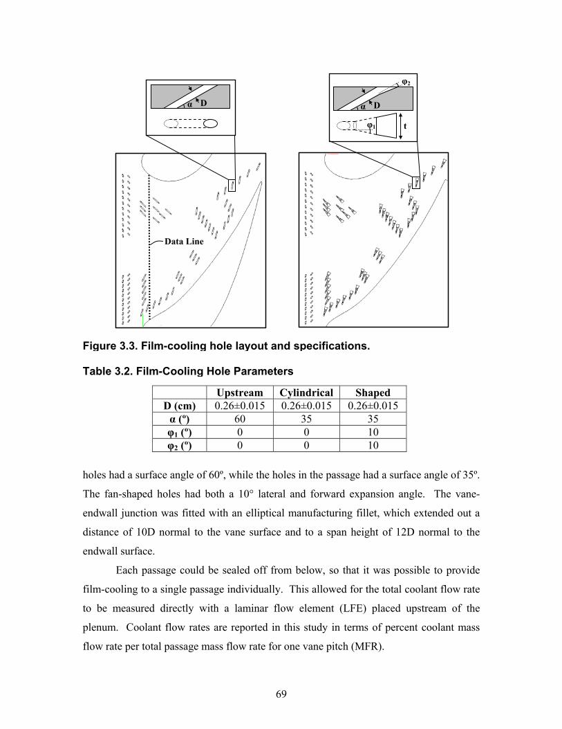
69

Upstream Cylindrical Shaped D (cm) 0.26±0.015 0.26±0.015 0.26±0.015 α (º) 60 35 35 φ1 (º) 0 0 10 φ2 (º) 0 0 10

holes had a surface angle of 60º, while the holes in the passage had a surface angle of 35º.

The fan-shaped holes had both a 10° lateral and forward expansion angle. The vane-

endwall junction was fitted with an elliptical manufacturing fillet, which extended out a

distance of 10D normal to the vane surface and to a span height of 12D normal to the

endwall surface.

Each passage could be sealed off from below, so that it was possible to provide

film-cooling to a single passage individually. This allowed for the total coolant flow rate

to be measured directly with a laminar flow element (LFE) placed upstream of the

plenum. Coolant flow rates are reported in this study in terms of percent coolant mass

flow rate per total passage mass flow rate for one vane pitch (MFR).


Figure 3.3. Film-cooling hole layout and specifications.

Data Line

α D

φ1 t

φ2

α D

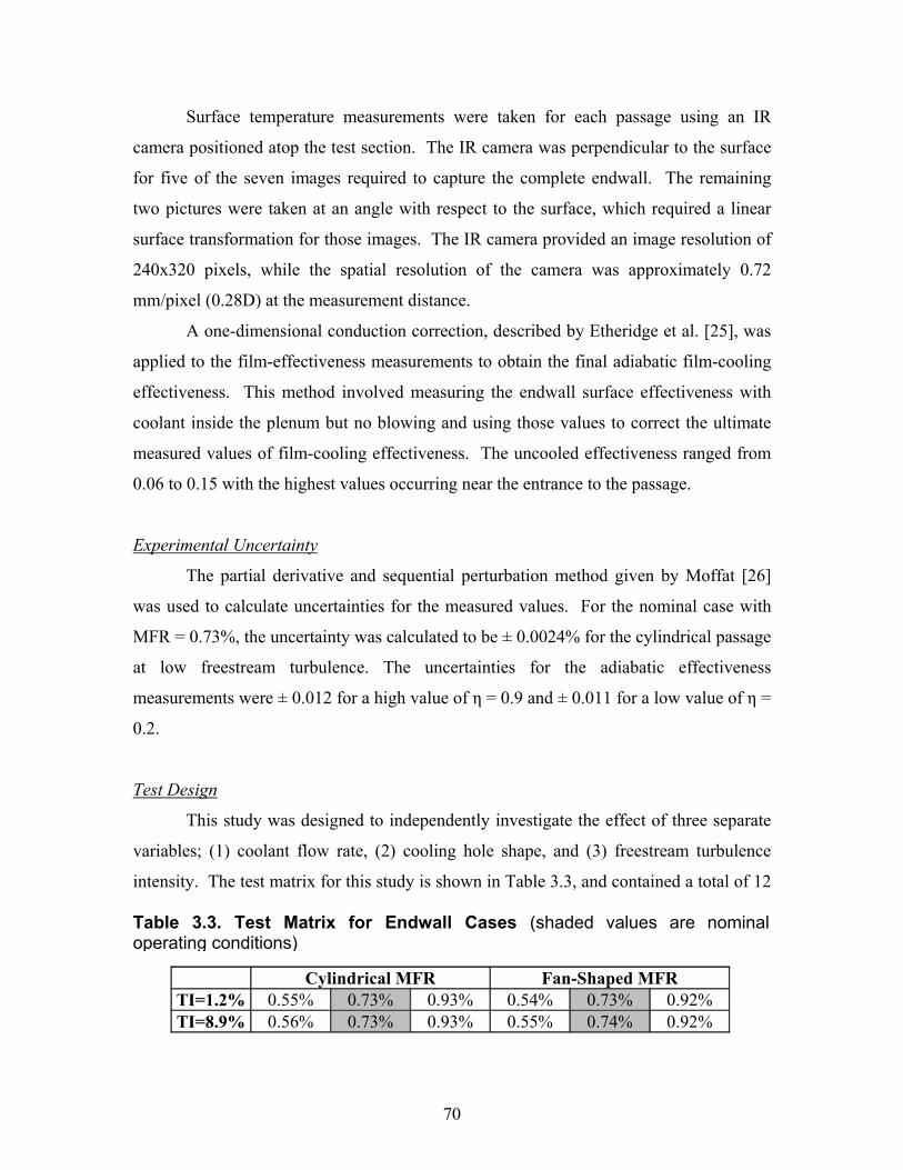
70

Surface temperature measurements were taken for each passage using an IR

camera positioned atop the test section. The IR camera was perpendicular to the surface

for five of the seven images required to capture the complete endwall. The remaining

two pictures were taken at an angle with respect to the surface, which required a linear

surface transformation for those images. The IR camera provided an image resolution of

240x320 pixels, while the spatial resolution of the camera was approximately 0.72

mm/pixel (0.28D) at the measurement distance.

A one-dimensional conduction correction, described by Etheridge et al. [25], was

applied to the film-effectiveness measurements to obtain the final adiabatic film-cooling

effectiveness. This method involved measuring the endwall surface effectiveness with

coolant inside the plenum but no blowing and using those values to correct the ultimate

measured values of film-cooling effectiveness. The uncooled effectiveness ranged from

0.06 to 0.15 with the highest values occurring near the entrance to the passage.


The partial derivative and sequential perturbation method given by Moffat [26]

was used to calculate uncertainties for the measured values. For the nominal case with

MFR = 0.73%, the uncertainty was calculated to be ± 0.0024% for the cylindrical passage

at low freestream turbulence. The uncertainties for the adiabatic effectiveness

measurements were ± 0.012 for a high value of η = 0.9 and ± 0.011 for a low value of η =

0.2.

Test Design

This study was designed to independently investigate the effect of three separate

variables; (1) coolant flow rate, (2) cooling hole shape, and (3) freestream turbulence

intensity. The test matrix for this study is shown in Table 3.3, and contained a total of 12

Cylindrical MFR Fan-Shaped MFR TI=1.2% 0.55% 0.73% 0.93% 0.54% 0.73% 0.92% TI=8.9% 0.56% 0.73% 0.93% 0.55% 0.74% 0.92%

Table 3.3. Test Matrix for Endwall Cases (shaded values are nominal operating conditions)

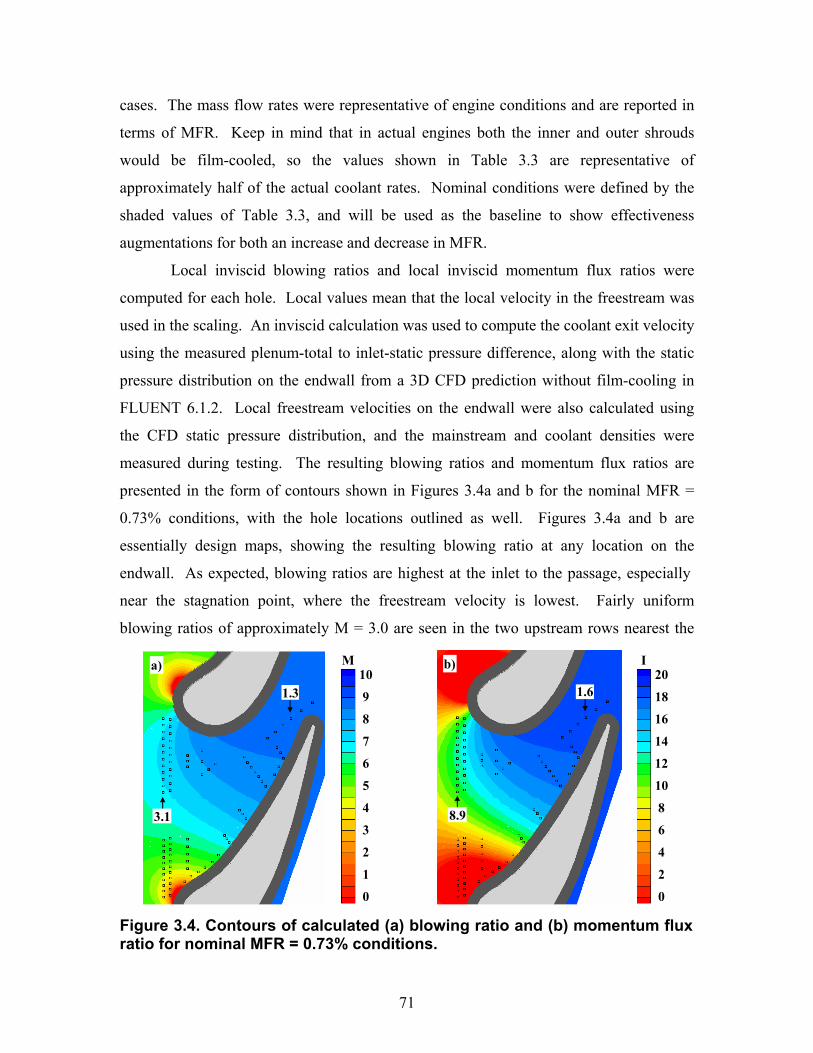
71

cases. The mass flow rates were representative of engine conditions and are reported in

terms of MFR. Keep in mind that in actual engines both the inner and outer shrouds

would be film-cooled, so the values shown in Table 3.3 are representative of

approximately half of the actual coolant rates. Nominal conditions were defined by the

shaded values of Table 3.3, and will be used as the baseline to show effectiveness

augmentations for both an increase and decrease in MFR.

Local inviscid blowing ratios and local inviscid momentum flux ratios were

computed for each hole. Local values mean that the local velocity in the freestream was

used in the scaling. An inviscid calculation was used to compute the coolant exit velocity

using the measured plenum-total to inlet-static pressure difference, along with the static

pressure distribution on the endwall from a 3D CFD prediction without film-cooling in

FLUENT 6.1.2. Local freestream velocities on the endwall were also calculated using

the CFD static pressure distribution, and the mainstream and coolant densities were

measured during testing. The resulting blowing ratios and momentum flux ratios are

presented in the form of contours shown in Figures 3.4a and b for the nominal MFR =

0.73% conditions, with the hole locations outlined as well. Figures 3.4a and b are

essentially design maps, showing the resulting blowing ratio at any location on the

endwall. As expected, blowing ratios are highest at the inlet to the passage, especially

near the stagnation point, where the freestream velocity is lowest. Fairly uniform

blowing ratios of approximately M = 3.0 are seen in the two upstream rows nearest the

b)

1.6

8.9

M10

9

8

7

6

5

4

3

2

1

0

I 20

18

16

14

12

10

8

6

4

2

0

1.3

3.1

a)

Figure 3.4. Contours of calculated (a) blowing ratio and (b) momentum fluxratio for nominal MFR = 0.73% conditions.

72

suction side, while the blowing ratios on the two upstream rows nearest the pressure side

vary from M = 2.8 to M = 5.9. The blowing ratios for the majority of the holes in the

passage are less than 2.0, as the flow accelerates to nearly five times the inlet velocity in

the throat region.

Experimental Results

Results are presented in terms of adiabatic film-cooling effectiveness. Contours

are shown in Figures 3.5a-f for the low freestream turbulence cases and in Figures 3.6a-f

for the high freestream turbulence cases. Analysis plots of laterally-averaged and area-

averaged effectiveness are also given along with film-effectiveness augmentation plots of

laterally-averaged effectiveness, which show the effects of blowing ratio, hole shape, and

freestream turbulence.

Cylindrical Holes at Low Freestream Turbulence

The adiabatic effectiveness contours for the cylindrical passage at low freestream

turbulence are shown in Figures 3.5a-c. Overall, effectiveness levels were very low,

especially in the region downstream of the double rows of holes at the entrance to the

passage, which had a steeper surface angle than the passage holes (60º as opposed to 35º

for the passage). Nearly all of the cooling flow from those two rows lifted off the surface,

which is not surprising considering that blowing ratios for these holes ranged from 2.8 to

5.9. Only for the lowest flowrate (MFR = 0.55%), were slight cooling footprints visible

downstream of the double cylindrical rows.

The row of pressure side holes running along the edge of the fillet just

downstream of the leading edge separated completely. Blowing ratios for the holes in

that region were extremely high between M = 3.9 and 8.5 (see Figure 3.4a), which is well

above the range for cylindrical jet attachement.

The majority of the cooling footprints showed individual jets, indicating that there

was not good lateral spreading downstream of most of the cylindrical holes. Most of the

holes had a hole-to-hole spacing of greater than five hole diameters, which is generally

too large to show significant jet merging. The exception was the first row of holes on the

pressure side (X/C = 0), which seemed to have relatively good lateral spreading despite a

73

Figure 3.5. Effectiveness contours at low freestream turbulence for thecylindrical passage (a-c) and fan-shaped passage (d-f).

MFR=0.73% 1.2% TI

e)

d) MFR=0.54% 1.2% TI

a) MFR=0.55% 1.2% TI

f) MFR=0.92% 1.2% TI

c) MFR=0.93% 1.2% TI

η1.0

0.9

0.8

0.7

0.6

0.5

0.4

0.3

0.2

0.1

0.0

MFR=0.73% 1.2% TI

80%

b)

60%

40%

20%

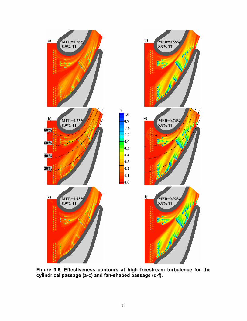
74

Figure 3.6. Effectiveness contours at high freestream turbulence for thecylindrical passage (a-c) and fan-shaped passage (d-f).

MFR=0.74% 8.9% TI

e)

d) MFR=0.55% 8.9% TI

a) MFR=0.56% 8.9% TI

f) MFR=0.92% 8.9% TI

c) MFR=0.93% 8.9% TI

η1.0

0.9

0.8

0.7

0.6

0.5

0.4

0.3

0.2

0.1

0.0

MFR=0.73% 8.9% TI

80%

b)

60%

40%

20%

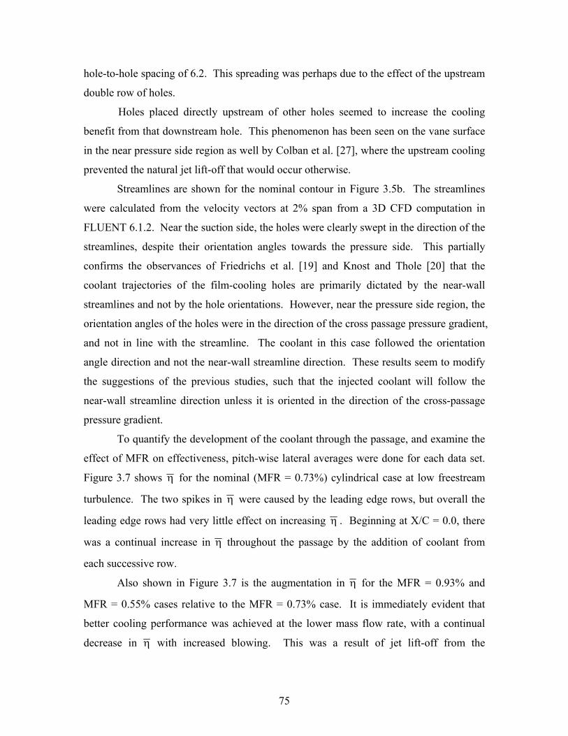
75

hole-to-hole spacing of 6.2. This spreading was perhaps due to the effect of the upstream

double row of holes.

Holes placed directly upstream of other holes seemed to increase the cooling

benefit from that downstream hole. This phenomenon has been seen on the vane surface

in the near pressure side region as well by Colban et al. [27], where the upstream cooling

prevented the natural jet lift-off that would occur otherwise.

Streamlines are shown for the nominal contour in Figure 3.5b. The streamlines

were calculated from the velocity vectors at 2% span from a 3D CFD computation in

FLUENT 6.1.2. Near the suction side, the holes were clearly swept in the direction of the

streamlines, despite their orientation angles towards the pressure side. This partially

confirms the observances of Friedrichs et al. [19] and Knost and Thole [20] that the

coolant trajectories of the film-cooling holes are primarily dictated by the near-wall

streamlines and not by the hole orientations. However, near the pressure side region, the

orientation angles of the holes were in the direction of the cross passage pressure gradient,

and not in line with the streamline. The coolant in this case followed the orientation

angle direction and not the near-wall streamline direction. These results seem to modify

the suggestions of the previous studies, such that the injected coolant will follow the

near-wall streamline direction unless it is oriented in the direction of the cross-passage

pressure gradient.

To quantify the development of the coolant through the passage, and examine the

effect of MFR on effectiveness, pitch-wise lateral averages were done for each data set.

Figure 3.7 shows η for the nominal (MFR = 0.73%) cylindrical case at low freestream

turbulence. The two spikes in η were caused by the leading edge rows, but overall the

leading edge rows had very little effect on increasing η . Beginning at X/C = 0.0, there

was a continual increase in η throughout the passage by the addition of coolant from

each successive row.

Also shown in Figure 3.7 is the augmentation in η for the MFR = 0.93% and

MFR = 0.55% cases relative to the MFR = 0.73% case. It is immediately evident that

better cooling performance was achieved at the lower mass flow rate, with a continual

decrease in η with increased blowing. This was a result of jet lift-off from the

76

0.0

0.1

0.2

0.3

0.4

0.5

0.0

0.5

1.0

1.5

2.0

-0.25 0.00 0.25 0.50

0.73% Coolant 0.93% Augmentation0.55% Augmentation

ηη

x.xx%

X/C

η0.73%

cylindrical holes. The same trend of increased cylindrical jet lift-off with increased

blowing ratio was also observed in the work done by Jabbari et al. [28].

Fan-Shaped Holes at Low Freestream Turbulence

The effectiveness contours for the fan-shaped passage at low turbulence are

shown in Figures 3.5d-f. It is immediately obvious that the fan-shaped cooling holes

provided much better cooling to the endwall than their cylindrical counterparts for the

same MFR. Specifically, the fan-shaped holes had much better lateral spreading, which

allowed the jets to stay attached to the surface because of the reduction in jet momentum.

It should be pointed out that the blowing ratios given in the contour in Figure 3.4a are

valid for the cylindrical metering area of fan-shaped holes, and that the effective blowing

ratio at the fan-shaped hole exit would be approximately half, corresponding to an area

ratio of two for the fan-shaped holes.

It is interesting to note that in the area of highest blowing ratio near the pressure

side leading edge next to the fillet some of the jets appear to be lifting off, just as in the

cylindrical passage. This seems to suggest that the lift-off in that region was not only due

Figure 3.7. Laterally averaged effectiveness for the 0.73% case andaugmentation of laterally averaged effectiveness for the 0.55% and 0.93%cases on the cylindrical passage.

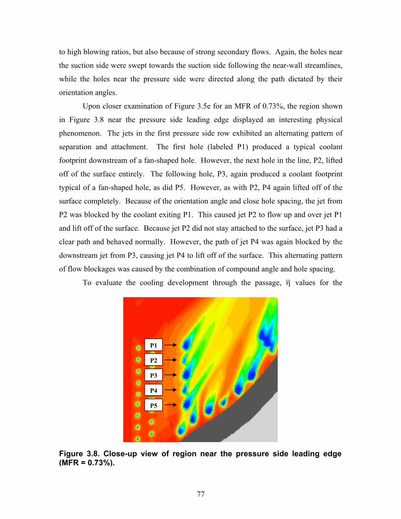
77

to high blowing ratios, but also because of strong secondary flows. Again, the holes near

the suction side were swept towards the suction side following the near-wall streamlines,

while the holes near the pressure side were directed along the path dictated by their

orientation angles.

Upon closer examination of Figure 3.5e for an MFR of 0.73%, the region shown

in Figure 3.8 near the pressure side leading edge displayed an interesting physical

phenomenon. The jets in the first pressure side row exhibited an alternating pattern of

separation and attachment. The first hole (labeled P1) produced a typical coolant

footprint downstream of a fan-shaped hole. However, the next hole in the line, P2, lifted

off of the surface entirely. The following hole, P3, again produced a coolant footprint

typical of a fan-shaped hole, as did P5. However, as with P2, P4 again lifted off of the

surface completely. Because of the orientation angle and close hole spacing, the jet from

P2 was blocked by the coolant exiting P1. This caused jet P2 to flow up and over jet P1

and lift off of the surface. Because jet P2 did not stay attached to the surface, jet P3 had a

clear path and behaved normally. However, the path of jet P4 was again blocked by the

downstream jet from P3, causing jet P4 to lift off of the surface. This alternating pattern

of flow blockages was caused by the combination of compound angle and hole spacing.

To evaluate the cooling development through the passage, η values for the

P1

P2

P3

P4

P5

Figure 3.8. Close-up view of region near the pressure side leading edge (MFR = 0.73%).

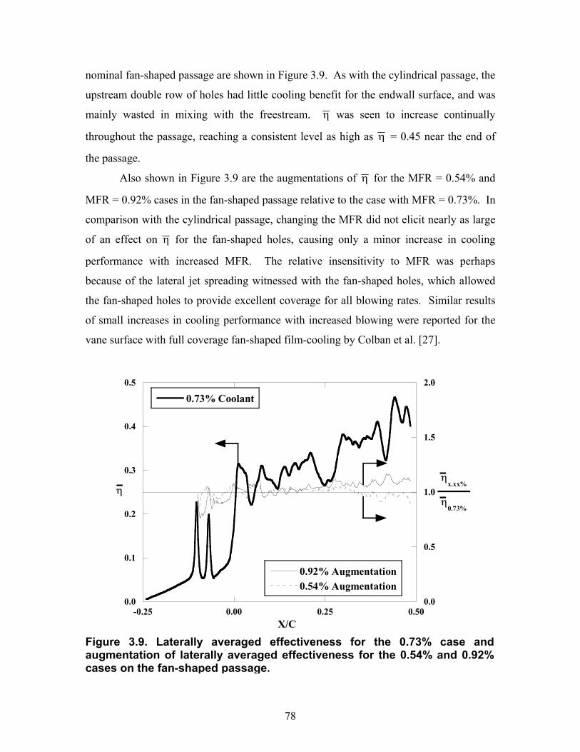
78

nominal fan-shaped passage are shown in Figure 3.9. As with the cylindrical passage, the

upstream double row of holes had little cooling benefit for the endwall surface, and was

mainly wasted in mixing with the freestream. η was seen to increase continually

throughout the passage, reaching a consistent level as high as η = 0.45 near the end of

the passage.

Also shown in Figure 3.9 are the augmentations of η for the MFR = 0.54% and

MFR = 0.92% cases in the fan-shaped passage relative to the case with MFR = 0.73%. In

comparison with the cylindrical passage, changing the MFR did not elicit nearly as large

of an effect on η for the fan-shaped holes, causing only a minor increase in cooling

performance with increased MFR. The relative insensitivity to MFR was perhaps

because of the lateral jet spreading witnessed with the fan-shaped holes, which allowed

the fan-shaped holes to provide excellent coverage for all blowing rates. Similar results

of small increases in cooling performance with increased blowing were reported for the

vane surface with full coverage fan-shaped film-cooling by Colban et al. [27].

0.0

0.1

0.2

0.3

0.4

0.5

0.0

0.5

1.0

1.5

2.0

-0.25 0.00 0.25 0.50

0.73% Coolant

0.92% Augmentation0.54% Augmentation

ηη

x.xx%

X/C

η0.73%

Figure 3.9. Laterally averaged effectiveness for the 0.73% case andaugmentation of laterally averaged effectiveness for the 0.54% and 0.92%cases on the fan-shaped passage.

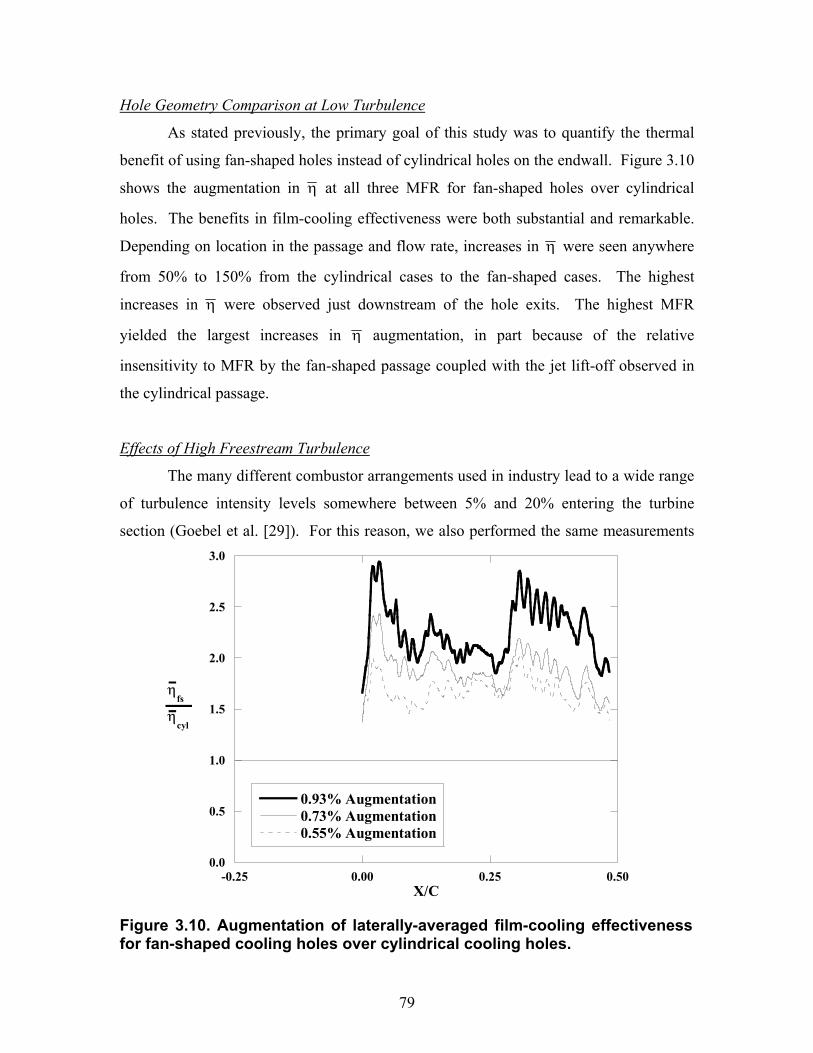
79

Hole Geometry Comparison at Low Turbulence

As stated previously, the primary goal of this study was to quantify the thermal

benefit of using fan-shaped holes instead of cylindrical holes on the endwall. Figure 3.10

shows the augmentation in η at all three MFR for fan-shaped holes over cylindrical

holes. The benefits in film-cooling effectiveness were both substantial and remarkable.

Depending on location in the passage and flow rate, increases in η were seen anywhere

from 50% to 150% from the cylindrical cases to the fan-shaped cases. The highest

increases in η were observed just downstream of the hole exits. The highest MFR

yielded the largest increases in η augmentation, in part because of the relative

insensitivity to MFR by the fan-shaped passage coupled with the jet lift-off observed in

the cylindrical passage.

Effects of High Freestream Turbulence

The many different combustor arrangements used in industry lead to a wide range

of turbulence intensity levels somewhere between 5% and 20% entering the turbine

section (Goebel et al. [29]). For this reason, we also performed the same measurements

0.0

0.5

1.0

1.5

2.0

2.5

3.0

-0.25 0.00 0.25 0.50

0.93% Augmentation0.73% Augmentation0.55% Augmentation

X/C

ηfs

ηcyl

Figure 3.10. Augmentation of laterally-averaged film-cooling effectiveness for fan-shaped cooling holes over cylindrical cooling holes.

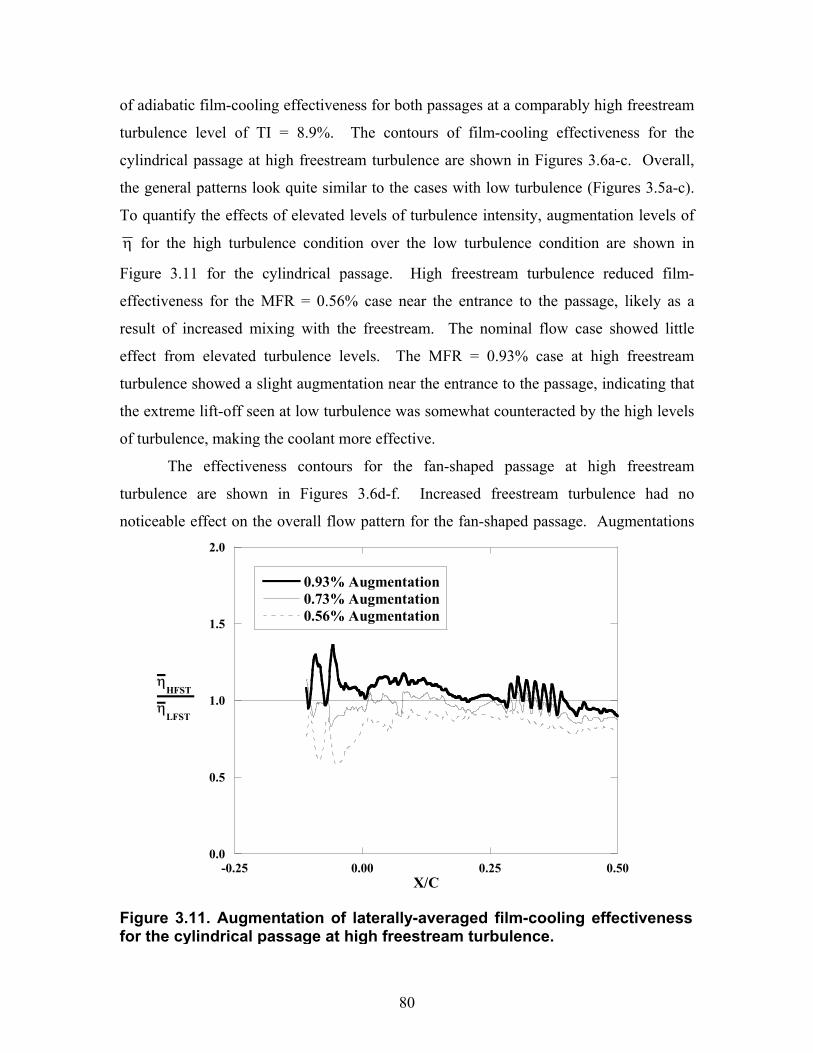
80

of adiabatic film-cooling effectiveness for both passages at a comparably high freestream

turbulence level of TI = 8.9%. The contours of film-cooling effectiveness for the

cylindrical passage at high freestream turbulence are shown in Figures 3.6a-c. Overall,

the general patterns look quite similar to the cases with low turbulence (Figures 3.5a-c).

To quantify the effects of elevated levels of turbulence intensity, augmentation levels of

η for the high turbulence condition over the low turbulence condition are shown in

Figure 3.11 for the cylindrical passage. High freestream turbulence reduced film-

effectiveness for the MFR = 0.56% case near the entrance to the passage, likely as a

result of increased mixing with the freestream. The nominal flow case showed little

effect from elevated turbulence levels. The MFR = 0.93% case at high freestream

turbulence showed a slight augmentation near the entrance to the passage, indicating that

the extreme lift-off seen at low turbulence was somewhat counteracted by the high levels

of turbulence, making the coolant more effective.

The effectiveness contours for the fan-shaped passage at high freestream

turbulence are shown in Figures 3.6d-f. Increased freestream turbulence had no

noticeable effect on the overall flow pattern for the fan-shaped passage. Augmentations

0.0

0.5

1.0

1.5

2.0

-0.25 0.00 0.25 0.50

0.93% Augmentation0.73% Augmentation0.56% Augmentation

X/C

ηHFST

ηLFST

Figure 3.11. Augmentation of laterally-averaged film-cooling effectiveness for the cylindrical passage at high freestream turbulence.

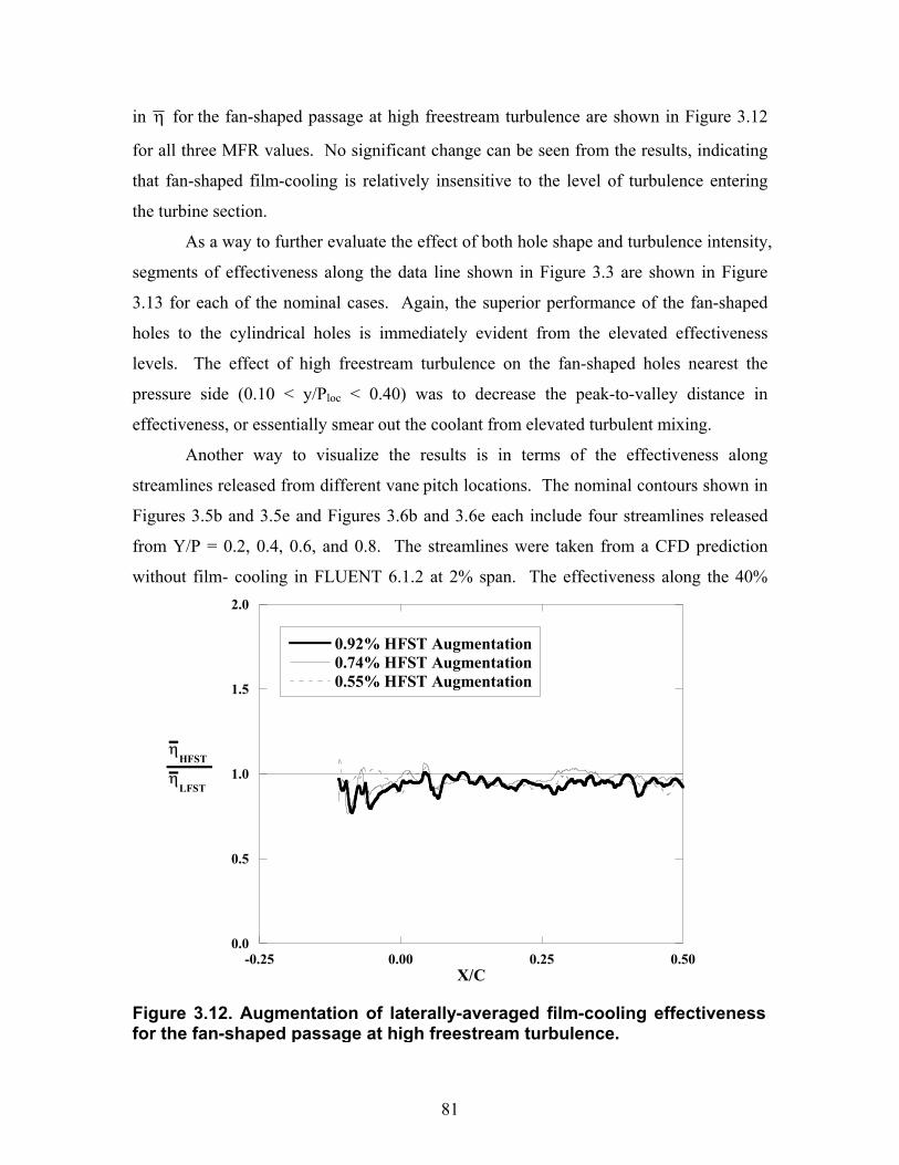
81

in η for the fan-shaped passage at high freestream turbulence are shown in Figure 3.12

for all three MFR values. No significant change can be seen from the results, indicating

that fan-shaped film-cooling is relatively insensitive to the level of turbulence entering

the turbine section.

As a way to further evaluate the effect of both hole shape and turbulence intensity,

segments of effectiveness along the data line shown in Figure 3.3 are shown in Figure

3.13 for each of the nominal cases. Again, the superior performance of the fan-shaped

holes to the cylindrical holes is immediately evident from the elevated effectiveness

levels. The effect of high freestream turbulence on the fan-shaped holes nearest the

pressure side (0.10 < y/Ploc < 0.40) was to decrease the peak-to-valley distance in

effectiveness, or essentially smear out the coolant from elevated turbulent mixing.

Another way to visualize the results is in terms of the effectiveness along

streamlines released from different vane pitch locations. The nominal contours shown in

Figures 3.5b and 3.5e and Figures 3.6b and 3.6e each include four streamlines released

from Y/P = 0.2, 0.4, 0.6, and 0.8. The streamlines were taken from a CFD prediction

without film- cooling in FLUENT 6.1.2 at 2% span. The effectiveness along the 40%

0.0

0.5

1.0

1.5

2.0

-0.25 0.00 0.25 0.50

0.92% HFST Augmentation0.74% HFST Augmentation0.55% HFST Augmentation

X/C

ηHFST

ηLFST

Figure 3.12. Augmentation of laterally-averaged film-cooling effectiveness for the fan-shaped passage at high freestream turbulence.

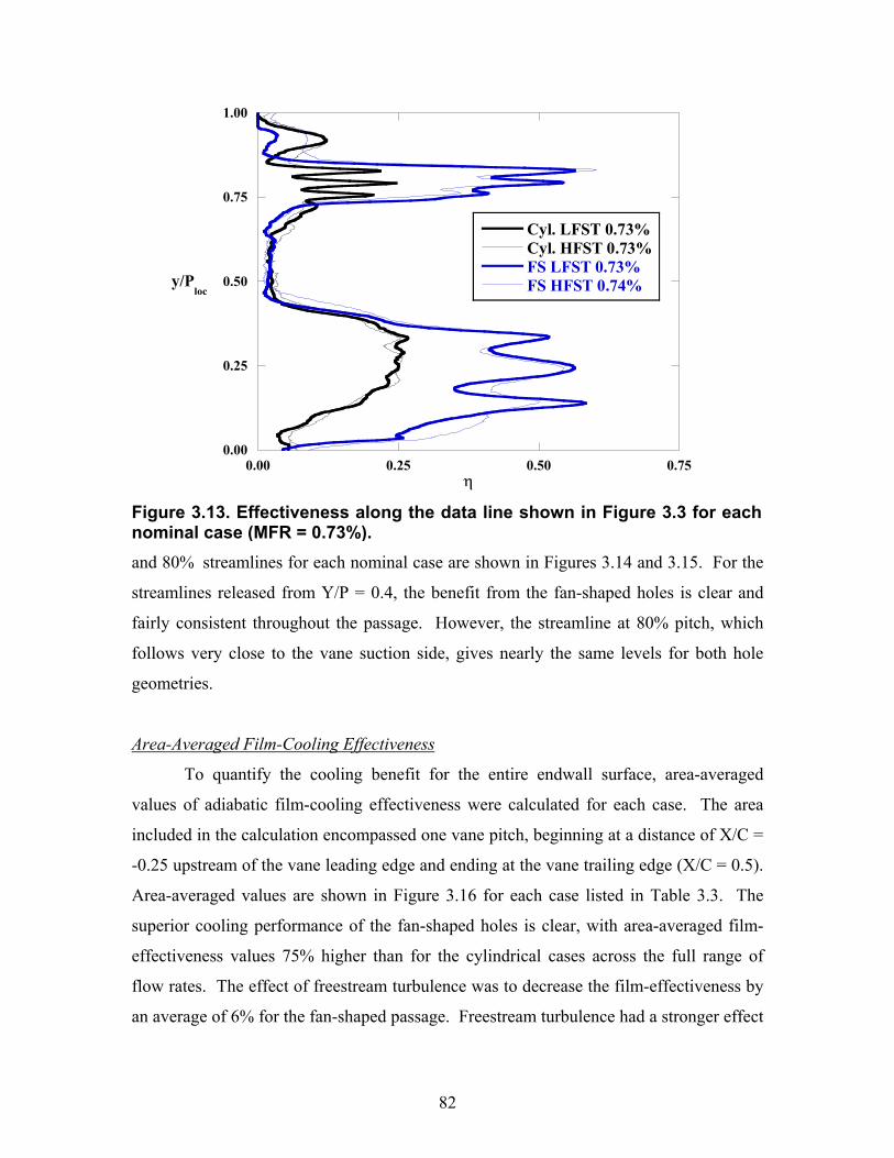
82

0.00

0.25

0.50

0.75

1.00

0.00 0.25 0.50 0.75

Cyl. LFST 0.73%Cyl. HFST 0.73%FS LFST 0.73%FS HFST 0.74%y/P

loc

η

and 80% streamlines for each nominal case are shown in Figures 3.14 and 3.15. For the

streamlines released from Y/P = 0.4, the benefit from the fan-shaped holes is clear and

fairly consistent throughout the passage. However, the streamline at 80% pitch, which

follows very close to the vane suction side, gives nearly the same levels for both hole

geometries.

Area-Averaged Film-Cooling Effectiveness

To quantify the cooling benefit for the entire endwall surface, area-averaged

values of adiabatic film-cooling effectiveness were calculated for each case. The area

included in the calculation encompassed one vane pitch, beginning at a distance of X/C =

-0.25 upstream of the vane leading edge and ending at the vane trailing edge (X/C = 0.5).

Area-averaged values are shown in Figure 3.16 for each case listed in Table 3.3. The

superior cooling performance of the fan-shaped holes is clear, with area-averaged film-

effectiveness values 75% higher than for the cylindrical cases across the full range of

flow rates. The effect of freestream turbulence was to decrease the film-effectiveness by

an average of 6% for the fan-shaped passage. Freestream turbulence had a stronger effect

Figure 3.13. Effectiveness along the data line shown in Figure 3.3 for eachnominal case (MFR = 0.73%).

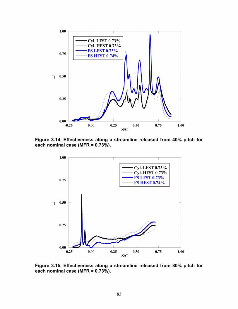
83

0.00

0.25

0.50

0.75

1.00

-0.25 0.00 0.25 0.50 0.75 1.00

Cyl. LFST 0.73%Cyl. HFST 0.73%FS LFST 0.73%FS HFST 0.74%

η

S/C

0.00

0.25

0.50

0.75

1.00

-0.25 0.00 0.25 0.50 0.75 1.00

Cyl. LFST 0.73%Cyl. HFST 0.73%FS LFST 0.73%FS HFST 0.74%

η

S/C

Figure 3.15. Effectiveness along a streamline released from 80% pitch foreach nominal case (MFR = 0.73%).

Figure 3.14. Effectiveness along a streamline released from 40% pitch foreach nominal case (MFR = 0.73%).

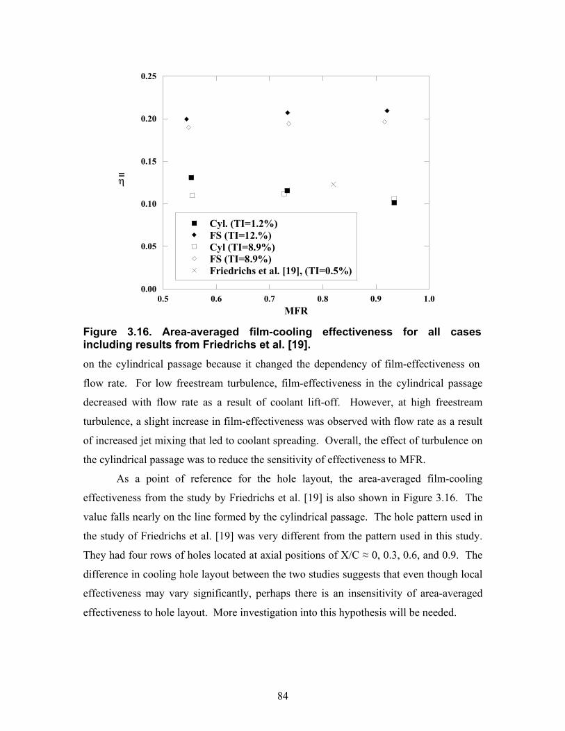
84

0.00

0.05

0.10

0.15

0.20

0.25

0.5 0.6 0.7 0.8 0.9 1.0

Cyl. (TI=1.2%)FS (TI=12.%)Cyl (TI=8.9%)FS (TI=8.9%)Friedrichs et al. [19], (TI=0.5%)

MFR

η

on the cylindrical passage because it changed the dependency of film-effectiveness on

flow rate. For low freestream turbulence, film-effectiveness in the cylindrical passage

decreased with flow rate as a result of coolant lift-off. However, at high freestream

turbulence, a slight increase in film-effectiveness was observed with flow rate as a result

of increased jet mixing that led to coolant spreading. Overall, the effect of turbulence on

the cylindrical passage was to reduce the sensitivity of effectiveness to MFR.

As a point of reference for the hole layout, the area-averaged film-cooling

effectiveness from the study by Friedrichs et al. [19] is also shown in Figure 3.16. The

value falls nearly on the line formed by the cylindrical passage. The hole pattern used in

the study of Friedrichs et al. [19] was very different from the pattern used in this study.

They had four rows of holes located at axial positions of X/C ≈ 0, 0.3, 0.6, and 0.9. The

difference in cooling hole layout between the two studies suggests that even though local

effectiveness may vary significantly, perhaps there is an insensitivity of area-averaged

effectiveness to hole layout. More investigation into this hypothesis will be needed.

Figure 3.16. Area-averaged film-cooling effectiveness for all cases including results from Friedrichs et al. [19].

85

Conclusions This paper has presented high resolution measurements of adiabatic film-cooling

effectiveness for both cylindrical and fan-shaped holes on a turbine vane endwall surface.

Results were presented at both high and low values of freestream turbulence. The

measurements were performed in a large-scale, low-speed, two-passage, linear turbine

vane cascade, with the identical cooling hole pattern in each passage but with different

hole shapes.

The major conclusion from this work was a superior performance of fan-shaped

holes in the platform region was found relative to cylindrical holes. An increase in film-

effectiveness of 75% based on area averages was seen by using fan-shaped holes instead

of cylindrical holes. The effect of high freestream turbulence was to reduce cooling

performance by 6% in the fan-shaped passage, and to change the dependency of film-

effectiveness on flow rate for the cylindrical passage.

Little benefit from a cooling standpoint was seen from the double row of

staggered cylindrical holes placed upstream of each passage. Further work is planned to

investigate the effect of the upstream blowing on the cooling performance of the

downstream holes. Work is also planned to compare the aerodynamic performance of the

two hole shapes.

Acknowledgments

The authors are grateful to Siemens Power Generation for their funding and


Nomenclature C true vane chord

Cp static pressure coefficient, Cp = (ps,loc – ps,in)/0.5ρinU2in


I local momentum flux ratio, I = ρcUc2/ρinUin

2


M local blowing ratio, M = ρcUc/ρinUin

MFR % total coolant mass flow per total passage mass flow

86

p pressure

P vane pitch



s distance measured along a streamline

S streamwise distance around the vane

T temperature

TI turbulence intensity

U velocity

X axial coordinate measured from the vane stagnation

y local pitchwise coordinate

Y pitchwise coordinate

Greek


δ boundary layer thickness


η adiabatic film-cooling effectiveness

Λx integral length scale

ρ density



Subscripts

c coolant

cyl cylindrical holes

fs fan-shaped holes

HFST high freestream turbulence condition (TI = 8.9%)

in inlet condition

LFST low freestream turbulence condition (TI = 1.2%)

loc local value

87

max maximum value of given variable at that location

s static

Overbar

– lateral average

= area average

References [1] Bunker, R. S., "A Review of Shaped Hole Turbine Film-Cooling Technology,"


[2] Goldstein, R. J., Eckert, E. R. G., and Burggraf, F., "Effects of Hole Geometry

and Density on Three-Dimensional Film Cooling," ASME Journal of Heat and

Mass Transfer, vol. 17, pp. 595-607, 1974.

[3] Kercher, D. M., Film-Cooling Bibliography: 1940-2002: Private publication,

2003.

[4] Kercher, D. M., Film-Cooling Bibliography Addendum: 1999-2004: Private

publication, 2005.

[5] Goldstein, R. J., "Film Cooling," Advances in Heat Transfer, vol. 7, pp. 321-379,

1971.

[6] Bogard, D. G. and Thole, K. A., "Gas Turbine Film Cooling," to appear in the

AIAA Journal of Propulsion, 2006.

[7] Vogel, G., Wagner, G., and Bölcs, A., "Transient Liquid Crystal Technique

Combined with PSP for Improved Film Cooling Measurements," The 10th

International Symposium on Flow Visualization, vol. F0109, 2002.

88

[8] Vogel, G., "Experimental Study on a Heavy Film Cooled Nozzle Guide Vane

with Contoured Platforms," PhD Dissertation, École Polytechnique Fédérale de

Lausanne, 2002.

[9] Barigozzi, G., Benzoni, G., Franchini, G., and Perdichizzi, A., "Fan-Shaped Hole

Effects on the Aero-Thermal Performance of a Film Cooled Endwall," GT2005-

68544, 2005.

[10] Blair, M. F., "An Experimental Study of Heat Transfer and Film Cooling on

Large-Scale Turbine Endwalls," ASME Journal of Heat Transfer, vol. 96, pp.

524-529, 1974.

[11] Granser, D. and Schulenberg, T., "Prediction and Measurement of Film Cooling

Effectiveness for a First Stage Turbine Vane Shroud," 90-GT-95, 1990.

[12] Colban, W., Thole, K. A., and Zess, G., "Combustor Turbine Interface Studies -

Part 1: Endwall Effectiveness Measurements," ASME Journal of Turbomachinery,

vol. 125, pp. 193-202, 2003.

[13] Knost, D. G. and Thole, K. A., "Computational Predictions of Endwall Film-

Cooling for a First Stage Vane," GT2003-38252, 2003.

[14] Harasgama, S. P. and Burton, C. D., "Film Cooling Research on the Endwall of a

Turbine Nozzle Guide Vane in a Short Duration Annular Cascade: Part 1-

Experimental Technique and Results," ASME Journal of Turbomachinery, vol.

114, pp. 734-740, 1992.

[15] Nicklas, M., "Film-Cooled Turbine Endwall in a Transonic Flow Field: Part II -

Heat Transfer and Film-Cooling Effectiveness," 2001-GT-0146, 2001.

[16] Sieverding, C. H. and Wilputte, P., "Influence of Mach Number and Endwall

89

Cooling on Secondary Flows in a Straight Nozzle Cascade," ASME Journal of

Engineering for Gas Turbines and Power, vol. 103, pp. 257-264, 1981.

[17] Kost, F. and Nicklas, M., "Film-Cooled Turbine Endwall in a Transonic Flow

Field: Part I - Aerodynamic Measurements," 2001-GT-0145, 2001.

[18] Colban, W., Lethander, A. T., Thole, K. A., and Zess, G., "Combustor Turbine

Interface Studies - Part 2: Flow and Thermal Field Measurements," ASME

Journal of Turbomachinery, vol. 125, pp. 203-209, 2003.

[19] Friedrichs, S., Hodson, H. P., and Dawes, W. N., "Distribution of Film-Cooling

Effectiveness on a Turbine Endwall Measured Using the Ammonia and Diazo

Technique," ASME Journal of Turbomachinery, vol. 118, pp. 613-621, 1995.

[20] Knost, D. G. and Thole, K. A., "Adiabatic Effectiveness Measurements of

Endwall Film-Cooling for a First Stage Vane," ASME Journal of Turbomachinery,

vol. 127, pp. 297-305, 2005.

[21] Oke, R. A., Burd, S. W., Simon, T. W., and Vahlberg, R., "Measurements in a

Turbine Cascade over a Contoured Endwall: Discrete Hole Injection of Bleed

Flow," 2000-GT-214, 2000.

[22] Zhang, L. J. and Jaiswal, R. S., "Turbine Nozzle Endwall Film Cooling Study

Using Pressure-Sensitive Paint," ASME Journal of Turbomachinery, vol. 123, pp.

730-738, 2001.

[23] Zhang, L. and Moon, H. K., "Turbine Nozzle Endwall Inlet Film Cooling - The

Effect of a Back-Facing Step," GT2003-38319, 2003.

[24] Colban, W., Gratton, A., Thole, K. A., and Haendler, M., "Heat Transfer and

Film-Cooling Measurements on a Stator Vane with Fan-Shaped Cooling Holes,"

90

GT2005-68258, 2005.

[25] Ethridge, M. I., Cutbirth, J. M., and Bogard, D. G., "Scaling of Performance for

Varying Density Ratio Coolants on an Airfoil with Strong Curvature and Pressure

Gradient Effects," 2000-GT-239, 2000.

[26] Moffat, R. J., "Describing the Uncertainties in Experimental Results,"


[27] Colban, W., Thole, K. A., and Haendler, M., "Experimental and Computational

Comparisons of Fan-Shaped Film-Cooling on a Turbine Vane Surface,"

IMECE2005-79596, 2005.

[28] Jabbari, M. Y., Marston, K. C., Eckert, E. R. G., and Goldstein, R. J., "Film

Cooling of the Gas Turbine Endwall by Discrete-Hole Injection," 94-GT-67, 1994.

[29] Goebel, S. G., Abauf, N., Lovett, J. A., and Lee, C.-P., "Measurements of

Combustor Velocity and Turbulence Profiles," 93-GT-228, 1993.



Holes on a Vane Endwall with and without Upstream Blowing

To be submitted to the 2007 ASME Turbo Expo*

Abstract In the push for more efficient and powerful gas turbines, combustor exit

temperatures continue to rise. This requires active cooling for the downstream turbine

section to avoid thermal failure. Film-cooling has long been an integral part of turbine

cooling schemes. Cooling the endwall is particularly difficult as much of the coolant is

swept across the passage endwall by secondary flows.

This study investigated the effect of upstream blowing from two rows of film-

cooling holes on the endwall secondary flows. Flow-field measurements are presented at

the passage exit plane both with and without blowing from the upstream rows. Adiabatic

effectiveness measurements of the endwall surface are also presented to quantify the

cooling performance with and without upstream blowing. Two commonly used film-

cooling hole geometries were investigated; cylindrical holes in one passage and fan-

shaped holes in the other passage.

Results showed that film-cooling increases the aerodynamic losses at the exit

plane, with fan-shaped holes showing lower losses than cylindrical holes. Fan-shaped

holes also provided better adiabatic film-cooling effectiveness on the endwall than

cylindrical holes. In general, upstream blowing increased aerodynamic losses, due to the

increased mixing with the freestream. Although the upstream blowing did not show an

immediate benefit near the injection location because of separation, a significant cooling

benefit was observed further downstream for the passage film-cooling holes because of

the large amount of coolant in the passage from the upstream holes.

92

Introduction Increasing energy demands require more powerful and more efficient industrial

gas turbine engines. One means of achieving this goal is to increase the combustion

temperature, resulting in higher temperatures at the inlet of the turbine. Although this is

beneficial in terms of power output, it is anything but beneficial in terms of part life.

Turbine inlet temperatures are so high in today’s gas turbine engines that in the absence

of complex cooling schemes the turbine components would completely melt. Ultimately,

engine designers aim to accomplish two seemingly opposed tasks; to provide better

cooling to the critical surfaces while at the same time reducing the total amount of

coolant used. Coolant comes at a cost to an engine’s overall efficiency, as it is bled from

one of the compressor stages (the necessary injection pressure and temperature determine

exactly which compressor stage), so there is a trade-off in the cooling scheme design

process.

In addition to the high operating temperatures, the endwall platform region

typically has secondary flows, which tend to sweep coolant flow away from critical

surfaces and replace it with hot mainstream gases. Methods of reducing harmful

secondary flows include endwall profiling, upstream injection, and endwall contouring.

Morris and Hoare [1] showed that with a single contoured endwall, similar to this study,

the secondary flow losses near the flat endwall were reduced, while the secondary flow

losses near the contoured endwall were increased. A reduction in secondary flows

resulting from endwall contouring follows from an analysis of the static pressure

distribution around the vane. Implementing a contoured endwall pushes the minimum

static pressure towards the trailing edge, causing the airfoil to be more aft-loaded and

ultimately delaying the onset of the development of secondary flows.

Another method that has been used to try and diminish the strength of secondary

flows is to implement coolant ejection upstream of the first vane row. Coolant ejection

reenergizes the boundary layer and reduces the strength of the pressure gradients that lead

to the formation of passage secondary flows. Although the main purpose of the high-

momentum high-angle upstream injection is to actively control the formation of

secondary flows, that injection can also provide some additional cooling benefit.

The purpose of this study was two-fold. The first goal was to investigate the

93

effect of coolant injection on the development of the passage secondary flows. The

second objective was to quantitatively evaluate the effect of hole geometry on the exit

plane flowfield as well as the cooling performance on the endwall. A five-hole total

pressure probe was used to measure total pressure losses and all three velocity

components at the passage exit plane for cases with and without upstream injection. Also,

endwall adiabatic film-cooling effectiveness was measured using an infrared camera with

and without upstream injection. Two different cooling designs were investigated – one

with cylindrical holes and the other with fan-shaped holes – in order to compare the

relative performance of two different commonly used hole geometries.

Past Studies Because of the absolute necessity of effective turbine cooling in gas turbine

engines, film-cooling has been researched exhaustively for the last 50 years (Kercher [2],

[3]). Among the topics studied are hole geometry variations and internal and external

conditions such as blowing ratio, density ratio, turbulence level, surface curvature,

pressure gradient, cross-flow (internal and external), surface roughness, and hole location.

Two excellent reviews on the development of film-cooling technology over the years are

offered by Goldstein [4] and Bogard and Thole [5], with a third more specific review for

shaped film-cooling holes by Bunker [6]. In terms of hole location, the endwall region is

a particularly difficult region for film-cooling designers, partly because of secondary

flows, but also partly because of manufacturing difficulties.

Perhaps the most difficult obstacle facing film-cooling designers in the endwall

region is the cross-passage flow. The pressure gradient that develops across the passage

from the pressure to suction sides has severe cooling consequences. Coolant is swept

away from the near wall region, exposing the endwall surface to hot gas flow. This effect

has been documented for upstream slot flow cooling by Blair [7], Granser and

Schulenberg [8], Colban et al. [9], Knost and Thole [10], and Knost and Thole [11].

Other studies, such as those by Harasgama and Burton [12] and Nicklas [13], have also

verified this effect for endwall film-cooling located in the vane passage.

In addition to the thermal penalties associated with the nozzle guide vane

secondary flows, there are also aerodynamic penalties that accompany secondary flows in

94

the form of total pressure losses and non-uniform flow turning. Langston et al. [14], in a

study performed without endwall blowing, showed a significant loss in total pressure

corresponding to the center of the passage vortex as it migrated through the passage.

They showed that at the exit plane, the location of the passage vortex and the

corresponding loss core had migrated to the suction side of the vane and had risen off of

the endwall.

A number of studies, including Sieverding and Wilputte [15], Friedrichs et al.

[16], Kost and Nicklas [17], and Barigozzi et al. [18] have reported aerodynamic benefits

associated with endwall film-cooling in the form of reduction of the size and strength of

the passage vortex and a reduction in strength of the cross passage flow. However, there

is an aerodynamic downside to film-cooling injection, as Friedrichs et al. [19] reported

that film-cooling ultimately increases the total pressure losses through the passage. They

showed that the additional losses generated within the hole and the losses generated by

coolant mixing with the freestream outweigh the reduction in losses associated with a

reduction in secondary flows.

Both passive and active solutions to the problems associated with passage

secondary flows are being implemented into nozzle guide vanes. Passive solutions

include endwall contouring (Oke et al. [20]) and leading edge fillet designs, such as those

presented by Zess and Thole [21], Lethander and Thole [22], Becz et al. [23], and

Mahmood et al. [24]. One active solution that is currently employed in some designs is

to inject high momentum coolant upstream of the vane passage, in many cases in a

double row staggered configuration. Zhang and Jaiswal [25] measured endwall film-

cooling effectiveness on an endwall downstream of two staggered rows of 45º cylindrical

holes placed upstream of the vane passage. They showed that at low injection rates the

coolant was swept towards the suction side, indicating a strong cross-passage flow. As

the injection rate was increased, the cross-passage flow was diminished, and a more

complete cooling coverage was seen on the endwall. Using 30º cylindrical holes

upstream of a contoured endwall, Zhang and Moon [26] showed similar results, showing

less cross-passage flow at higher injection rates.

A study comparing total pressure losses between an uncooled endwall, a cooled

endwall with cylindrical holes, and a cooled endwall with shaped holes was performed by

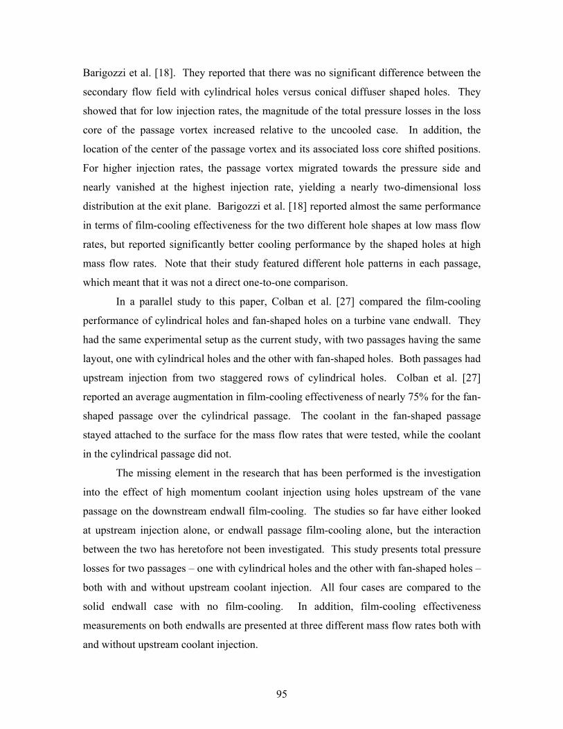
95

Barigozzi et al. [18]. They reported that there was no significant difference between the

secondary flow field with cylindrical holes versus conical diffuser shaped holes. They

showed that for low injection rates, the magnitude of the total pressure losses in the loss

core of the passage vortex increased relative to the uncooled case. In addition, the

location of the center of the passage vortex and its associated loss core shifted positions.

For higher injection rates, the passage vortex migrated towards the pressure side and

nearly vanished at the highest injection rate, yielding a nearly two-dimensional loss

distribution at the exit plane. Barigozzi et al. [18] reported almost the same performance

in terms of film-cooling effectiveness for the two different hole shapes at low mass flow

rates, but reported significantly better cooling performance by the shaped holes at high

mass flow rates. Note that their study featured different hole patterns in each passage,

which meant that it was not a direct one-to-one comparison.

In a parallel study to this paper, Colban et al. [27] compared the film-cooling

performance of cylindrical holes and fan-shaped holes on a turbine vane endwall. They

had the same experimental setup as the current study, with two passages having the same

layout, one with cylindrical holes and the other with fan-shaped holes. Both passages had

upstream injection from two staggered rows of cylindrical holes. Colban et al. [27]

reported an average augmentation in film-cooling effectiveness of nearly 75% for the fan-

shaped passage over the cylindrical passage. The coolant in the fan-shaped passage

stayed attached to the surface for the mass flow rates that were tested, while the coolant

in the cylindrical passage did not.

The missing element in the research that has been performed is the investigation

into the effect of high momentum coolant injection using holes upstream of the vane

passage on the downstream endwall film-cooling. The studies so far have either looked

at upstream injection alone, or endwall passage film-cooling alone, but the interaction

between the two has heretofore not been investigated. This study presents total pressure

losses for two passages – one with cylindrical holes and the other with fan-shaped holes –

both with and without upstream coolant injection. All four cases are compared to the

solid endwall case with no film-cooling. In addition, film-cooling effectiveness

measurements on both endwalls are presented at three different mass flow rates both with

and without upstream coolant injection.

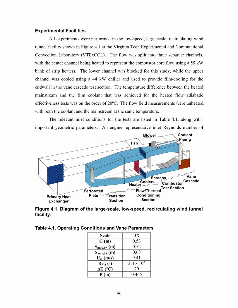
96

Experimental Facilities All experiments were performed in the low-speed, large scale, recirculating wind

tunnel facility shown in Figure 4.1 at the Virginia Tech Experimental and Computational

Convection Laboratory (VTExCCL). The flow was split into three separate channels,

with the center channel being heated to represent the combustor core flow using a 55 kW

bank of strip heaters. The lower channel was blocked for this study, while the upper

channel was cooled using a 44 kW chiller and used to provide film-cooling for the

endwall in the vane cascade test section. The temperature difference between the heated

mainstream and the film coolant that was achieved for the heated flow adiabatic

effectiveness tests was on the order of 20ºC. The flow field measurements were unheated,

with both the coolant and the mainstream at the same temperature.

The relevant inlet conditions for the tests are listed in Table 4.1, along with

important geometric parameters. An engine representative inlet Reynolds number of

Scale 3X C (m) 0.53

Smax,PS (m) 0.52 Smax,SS (m) 0.68 Uin (m/s) 9.41 Rein (-) 3.4 x 105 ∆T (ºC) 20 P (m) 0.465


Fan


HeaterCoolers

Screens


Section


Section


Vane Cascade

Figure 4.1. Diagram of the large-scale, low-speed, recirculating wind tunnel facility.


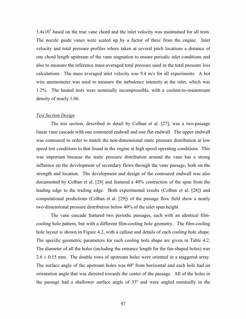
97

3.4x105 based on the true vane chord and the inlet velocity was maintained for all tests.

The nozzle guide vanes were scaled up by a factor of three from the engine. Inlet

velocity and total pressure profiles where taken at several pitch locations a distance of

one chord length upstream of the vane stagnation to ensure periodic inlet conditions and

also to measure the reference mass-averaged total pressure used in the total pressure loss

calculations. The mass averaged inlet velocity was 9.4 m/s for all experiments. A hot

wire anemometer was used to measure the turbulence intensity at the inlet, which was

1.2%. The heated tests were nominally incompressible, with a coolant-to-mainstream

density of nearly 1.06.

Test Section Design

The test section, described in detail by Colban et al. [27], was a two-passage

linear vane cascade with one contoured endwall and one flat endwall. The upper endwall

was contoured in order to match the non-dimensional static pressure distribution at low

speed test conditions to that found in the engine at high speed operating conditions. This

was important because the static pressure distribution around the vane has a strong

influence on the development of secondary flows through the vane passage, both on the

strength and location. The development and design of the contoured endwall was also

documented by Colban et al. [28] and featured a 40% contraction of the span from the

leading edge to the trailing edge. Both experimental results (Colban et al. [28]) and

computational predictions (Colban et al. [29]) of the passage flow field show a nearly

two-dimensional pressure distribution below 40% of the inlet span height.

The vane cascade featured two periodic passages, each with an identical film-

cooling hole pattern, but with a different film-cooling hole geometry. The film-cooling

hole layout is shown in Figure 4.2, with a callout and details of each cooling hole shape.

The specific geometric parameters for each cooling hole shape are given in Table 4.2.

The diameter of all the holes (including the entrance length for the fan-shaped holes) was

2.6 ± 0.15 mm. The double rows of upstream holes were oriented in a staggered array.

The surface angle of the upstream holes was 60º from horizontal and each hole had an

orientation angle that was directed towards the center of the passage. All of the holes in

the passage had a shallower surface angle of 35º and were angled nominally in the

98

Upstream Cylindrical Shaped D (cm) 0.26±0.015 0.26±0.015 0.26±0.015 α (º) 60 35 35 φ1 (º) 0 0 10 φ2 (º) 0 0 10

direction of the inviscid streamline at that location. The holes in the fan-shaped passage

also featured a lateral diffusion angle of 10º and a forward diffusion angle of 10º.

A single plenum, which provided coolant to supply the entire endwall, was

located beneath the test section. The capability was available to block off each passage

individually, as well as the rows of upstream holes, and measure exactly the amount of

coolant mass flow delivered to the entire endwall using a laminar flow element. The

amount of coolant in this study is reported in terms of mass flow rate (MFR), and is

defined as a percentage of the total passage mass flow rate for one vane pitch.

The endwall was constructed from a medium density foam material using a five-

axis water jet for high geometrical integrity of the hole design and pattern. The foam had

a low thermal conductivity (k = 0.028 W/m·K) such that the conduction losses laterally

Exit Plane

α D

φ1 t

φ2

α D

XY

Ψms

Ψms-Ψ

Vs,ms

VsVn


Figure 4.2. Film-cooling hole layout and specifications. Upstream injection holes are highlighted as well as the exit plane, which stretches from trailing edge to trailing edge.

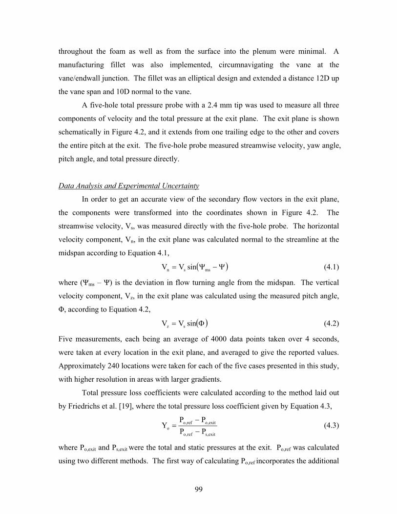
99

throughout the foam as well as from the surface into the plenum were minimal. A

manufacturing fillet was also implemented, circumnavigating the vane at the

vane/endwall junction. The fillet was an elliptical design and extended a distance 12D up

the vane span and 10D normal to the vane.

A five-hole total pressure probe with a 2.4 mm tip was used to measure all three

components of velocity and the total pressure at the exit plane. The exit plane is shown

schematically in Figure 4.2, and it extends from one trailing edge to the other and covers

the entire pitch at the exit. The five-hole probe measured streamwise velocity, yaw angle,

pitch angle, and total pressure directly.

Data Analysis and Experimental Uncertainty

In order to get an accurate view of the secondary flow vectors in the exit plane,

the components were transformed into the coordinates shown in Figure 4.2. The

streamwise velocity, Vs, was measured directly with the five-hole probe. The horizontal

velocity component, Vn, in the exit plane was calculated normal to the streamline at the

midspan according to Equation 4.1,

( )Ψ−Ψ= mssn sinVV (4.1)

where (Ψms – Ψ) is the deviation in flow turning angle from the midspan. The vertical

velocity component, Vz, in the exit plane was calculated using the measured pitch angle,

Φ, according to Equation 4.2,

( )Φ= sinVV sz (4.2)

Five measurements, each being an average of 4000 data points taken over 4 seconds,

were taken at every location in the exit plane, and averaged to give the reported values.

Approximately 240 locations were taken for each of the five cases presented in this study,

with higher resolution in areas with larger gradients.

Total pressure loss coefficients were calculated according to the method laid out

by Friedrichs et al. [19], where the total pressure loss coefficient given by Equation 4.3,

exit,sref,o

exit,oref,oo PP

PPY

−−

= (4.3)

where Po,exit and Ps,exit were the total and static pressures at the exit. Po,ref was calculated

using two different methods. The first way of calculating Po,ref incorporates the additional

100

total pressure and energy added to the passage flow as a result of the addition of film-

coolant. The mass-averaged calculation of Po,ref is given by Equation 4.4,

coolin

coolcool,oinin,oref,o

mm

mPmPP ⋅⋅

⋅⋅

+

+= (4.4)

The second definition used for Po,ref in Equation 4.4 was just to set Po,ref = Po,in, the mass-

averaged inlet stagnation pressure. This definition was used for the uncooled case, in

which case Equation 4.4 simplifies to that result, and was also calculated for the other

flowfield cases. The second definition neglects the total pressure additions from the film-

cooling flow, and can be misleading for that reason because it typically yields lower Yo

values than by using the definition for Po,ref in Equation 4.4.

Mass-averaged values of the total pressure loss coefficients were also computed

in the exit plane in order to give an overall comparison of each case in terms of complete

total pressure loss. The mass-averaging was done according to Equation 4.5,

∫ ∫

∫ ∫ρ

ρ=

Z Ys

Z Yso

o dYdZV

dYdZVYY (4.5)

although the density term cancelled out of Equation 4.5 because the tests were

incompressible, being unheated and at low speed.

Endwall surface temperatures were measured using an infrared camera and

converted to adiabatic film-cooling effectiveness. Eight image locations were necessary

to map the entire endwall surface for each passage. Five images were taken and averaged

at each location. A FLIR P20 infrared camera was used with an image resolution of 240

x 320 pixels, which gave an image resolution of approximately 0.28D per pixel. Each

image was calibrated using thermocouples embedded flush with the endwall surface, and

then corrected for conduction losses. A one-dimensional conduction correction was

applied to the measured film-cooling effectiveness to give the reported adiabatic film-

cooling effectiveness. The uncooled effectiveness, ηo, varied between 0.06 and 0.15, and

depended on the location on the endwall.

Uncertainty estimates were made using the technique described by Moffat [30],

which is a partial derivative and sequential perturbation method. The uncertainty in MFR

101

for the 0.73% case was determined to be ± 0.0024% for the cylindrical passage. This

value is representative of the other reported MFRs. A reported value of Yo = 0.15 for the

cylindrical passage with upstream blowing yielded an uncertainty of ± 0.001, with Po,ref

being the mass-averaged total pressure including coolant addition as defined by Equation

4.4. The uncertainty in adiabatic film-cooling effectiveness was also calculated for high

and low reported values. For a high value of η = 0.9, the uncertainty was ± 0.012, while

a lower value of η = 0.2 had an uncertainty of ± 0.011.

Test Design

The test matrix is shown in Table 4.3 and includes a total of 13 cases (baseline

case with no blowing is not shown). Adiabatic film-cooling effectiveness measurements

were made for all cases shown in Table 4.3. The cases for which flow field

measurements were taken at the exit plane are highlighted in the test matrix. One other

case was measured for the exit plane, and that was a case with no blowing, which was

meant to be a baseline case for the flow field measurements. Also, note both the inner

and outer endwalls are typically cooled in an actual engine, so the MFR values in Table

4.3 are representative of approximately half of the actual value per vane pitch. The

MFRs for the six cases without upstream injection were determined by matching the

pressure ratio between the endwall plenum total pressure and the vane stagnation total

pressure to the cases with upstream injection. In this way, the passage endwall film-

cooling holes had nominally the same MFR in both the upstream and no upstream

blowing cases.

To determine the distribution of blowing ratios and momentum ratios for the

endwall film-cooling holes, inviscid calculations were done using a computationally

predicted static pressure distribution on the endwall with no film-cooling along with the

Cylindrical Passage MFR Fan-Shaped Passage MFR

Upstream 0.55% 0.73% 0.93% 0.54% 0.73% 0.92%

No Upstream 0.36% 0.44% 0.55% 0.35% 0.45% 0.56%

Table 4.3. Test Matrix (shaded values indicate cases for which the exit planeflow field was measured)

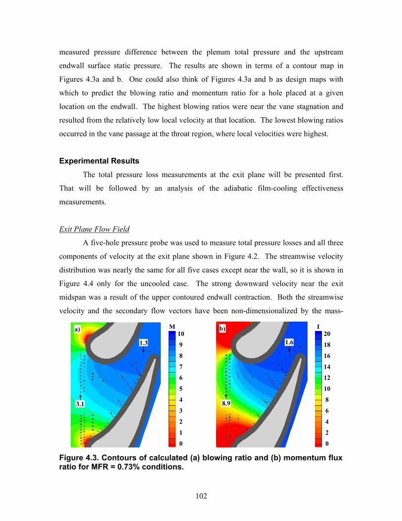
102

measured pressure difference between the plenum total pressure and the upstream

endwall surface static pressure. The results are shown in terms of a contour map in

Figures 4.3a and b. One could also think of Figures 4.3a and b as design maps with

which to predict the blowing ratio and momentum ratio for a hole placed at a given

location on the endwall. The highest blowing ratios were near the vane stagnation and

resulted from the relatively low local velocity at that location. The lowest blowing ratios

occurred in the vane passage at the throat region, where local velocities were highest.

Experimental Results The total pressure loss measurements at the exit plane will be presented first.

That will be followed by an analysis of the adiabatic film-cooling effectiveness

measurements.

Exit Plane Flow Field

A five-hole pressure probe was used to measure total pressure losses and all three

components of velocity at the exit plane shown in Figure 4.2. The streamwise velocity

distribution was nearly the same for all five cases except near the wall, so it is shown in

Figure 4.4 only for the uncooled case. The strong downward velocity near the exit

midspan was a result of the upper contoured endwall contraction. Both the streamwise

velocity and the secondary flow vectors have been non-dimensionalized by the mass-

Figure 4.3. Contours of calculated (a) blowing ratio and (b) momentum fluxratio for MFR = 0.73% conditions.

b)

1.6

8.9

M10

9

8

7

6

5

4

3

2

1

0

I 20

18

16

14

12

10

8

6

4

2

0

1.3

3.1

a)

103

averaged inlet velocity to the cascade. Figure 4.4 shows that the streamwise velocity is

nearly two-dimensional across most of the exit plane. There was a local minimum

nonuniformity in streamwise velocity corresponding to the location of the center of the

passage vortex near the suction side at Y/P = 0.9 and Z/P = 0.1. A strong cross passage

flow was seen near the wall from the pressure to the suction sides.

Normalized total pressure losses are shown in Figures 4.5a-e. For the baseline

uncooled case, the reference total pressure in Equation 4.3 was taken as the mass-

averaged inlet total pressure, while for the other cases, the reference total pressure was

mass-averaged including the coolant flow to incorporate the losses due to film-cooling

addition. Upon examining the uncooled case in Figure 4.5a, the most noticeable feature

was the loss core associated with the passage vortex, located at Y/P = 0.9 and Z/P = 0.1.

The passage vortex was the most dominant loss generator in the uncooled passage. As

with the streamwise velocity shown in Figure 4.4, the secondary flow vectors are

superimposed onto the total pressure loss contours in Figure 4.5a-e. There was also a

region of high losses near the endwall at the suction side corner. Langston et al. [14]

noticed the same phenomenon for an uncooled endwall and attributed it to the separation

of the endwall boundary layer.

Figure 4.5b shows the total pressure losses in the exit plane for the cylindrical

passage with upstream injection. Two major changes occurred from the uncooled case.

First, the location of the passage vortex shifted away from the suction side, perhaps due

Figure 4.4. Contour of streamwise velocity in the exit plane for theuncooled case with superimposed secondary flow vectors.

Vs/Uin

6.0

5.8

5.6

5.4

5.2

5.0

4.8

4.6

4.4

4.2

4.0

Z/P

Y/P

PS SS

U/Uin

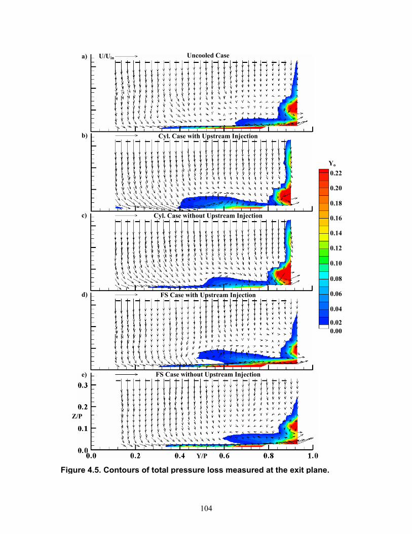
104

Figure 4.5. Contours of total pressure loss measured at the exit plane.

d)

a)

c)

b)

e)

Y/P

U/Uin Uncooled Case

Cyl. Case with Upstream Injection

Cyl. Case without Upstream Injection

FS Case with Upstream Injection

FS Case without Upstream Injection

Z/P

Yo

0.22

0.20

0.18

0.16

0.14

0.12

0.10

0.08

0.06

0.04

0.02 0.00

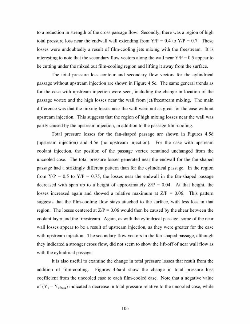
105

to a reduction in strength of the cross passage flow. Secondly, there was a region of high

total pressure loss near the endwall wall extending from Y/P = 0.4 to Y/P = 0.7. These

losses were undoubtedly a result of film-cooling jets mixing with the freestream. It is

interesting to note that the secondary flow vectors along the wall near Y/P = 0.5 appear to

be cutting under the mixed out film-cooling region and lifting it away from the surface.

The total pressure loss contour and secondary flow vectors for the cylindrical

passage without upstream injection are shown in Figure 4.5c. The same general trends as

for the case with upstream injection were seen, including the change in location of the

passage vortex and the high losses near the wall from jet/freestream mixing. The main

difference was that the mixing losses near the wall were not as great for the case without

upstream injection. This suggests that the region of high mixing losses near the wall was

partly caused by the upstream injection, in addition to the passage film-cooling.

Total pressure losses for the fan-shaped passage are shown in Figures 4.5d

(upstream injection) and 4.5e (no upstream injection). For the case with upstream

coolant injection, the position of the passage vortex remained unchanged from the

uncooled case. The total pressure losses generated near the endwall for the fan-shaped

passage had a strikingly different pattern than for the cylindrical passage. In the region

from Y/P = 0.5 to Y/P = 0.75, the losses near the endwall in the fan-shaped passage

decreased with span up to a height of approximately Z/P = 0.04. At that height, the

losses increased again and showed a relative maximum at Z/P = 0.06. This pattern

suggests that the film-cooling flow stays attached to the surface, with less loss in that

region. The losses centered at Z/P = 0.06 would then be caused by the shear between the

coolant layer and the freestream. Again, as with the cylindrical passage, some of the near

wall losses appear to be a result of upstream injection, as they were greater for the case

with upstream injection. The secondary flow vectors in the fan-shaped passage, although

they indicated a stronger cross flow, did not seem to show the lift-off of near wall flow as

with the cylindrical passage.

It is also useful to examine the change in total pressure losses that result from the

addition of film-cooling. Figures 4.6a-d show the change in total pressure loss

coefficient from the uncooled case to each film-cooled case. Note that a negative value

of (Yo – Yo,base) indicated a decrease in total pressure relative to the uncooled case, while

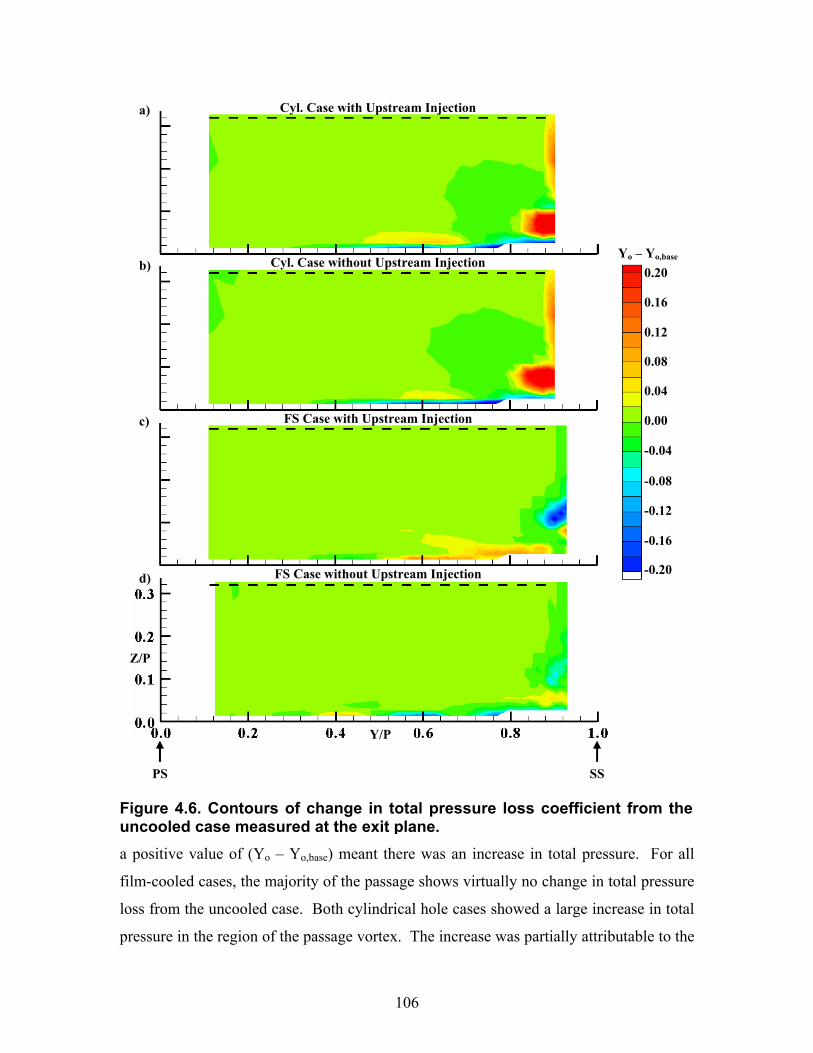
106

a positive value of (Yo – Yo,base) meant there was an increase in total pressure. For all

film-cooled cases, the majority of the passage shows virtually no change in total pressure

loss from the uncooled case. Both cylindrical hole cases showed a large increase in total

pressure in the region of the passage vortex. The increase was partially attributable to the

Figure 4.6. Contours of change in total pressure loss coefficient from theuncooled case measured at the exit plane.

Cyl. Case with Upstream Injection

Cyl. Case without Upstream Injection

FS Case with Upstream Injection

FS Case without Upstream Injectiond)

a)

c)

b)

Z/P

Y/P

PS SS

Yo – Yo,base

0.20

0.16

0.12

0.08

0.04

0.00

-0.04

-0.08

-0.12

-0.16

-0.20

107

shift in location of the loss core away from the suction surface for the two cylindrical

cases. However, it is likely that the maximum loss associated with the passage vortex

was also enhanced. Barigozzi et al. [18] also reported an increase in total pressure loss

generated by the passage vortex for a similar MFR with cylindrical hole film-cooling

relative to the uncooled case.

For the fan-shaped passage, (Yo – Yo,base) values increased for the upstream

injection case in the shear layer mixing region, as shown in Figure 4.6c. However, the

upstream injection seemed to reduce the losses associated with the passage vortex for the

fan-shaped case. The fan-shaped case without upstream cooling was the most similar to

the uncooled case in terms of total pressure loss. There was very little change in either

magnitude or distribution of the total pressure losses from the uncooled case to the fan-

shaped case without upstream injection, with only a slight reduction in losses associated

with the passage vortex and a slight increase in losses because of mixing and shear within

the passage.

Because the main purpose of the nozzle guide vanes is to turn the flow as it enters

the downstream first blade row, which extracts energy from the expanding hot gases, the

exit angle of the flow through the passage is extremely important. Secondary flows such

as the near wall cross flow decrease the overall efficiency of the engine because they alter

the exit flow angles. Engine designers would like to have as uniform an exit flow angle

as possible, or else the blade design must include these flow angles. Figure 4.7 shows

pitch-averaged flow angles at the exit plane for each of the five cases as the difference

from the midspan flow turning angle. The uncooled case had very little variation above

Z/Zmax = 0.1. Both fan-shaped cases had a similar distribution of flow-turning angles

along the span, with slightly higher turning near the wall. The cylindrical cases had

significantly less turning in the near wall region, which means that the endwall cross flow

was reduced. This corresponds to the shift in location of the passage vortex towards the

pressure side from the uncooled case (Figures 4.5a-c). Although the cylindrical passage

cases had less endwall cross flow, they did have a higher flow turning angle than the

uncooled case from Z/Zmax = 0.1 to Z/Zmax = 0.25. The difference in flow turning angles

between the uncooled cases and the cases with film-cooling stresses the importance of

incorporating the changes in flowfield that are brought upon by film injection into the

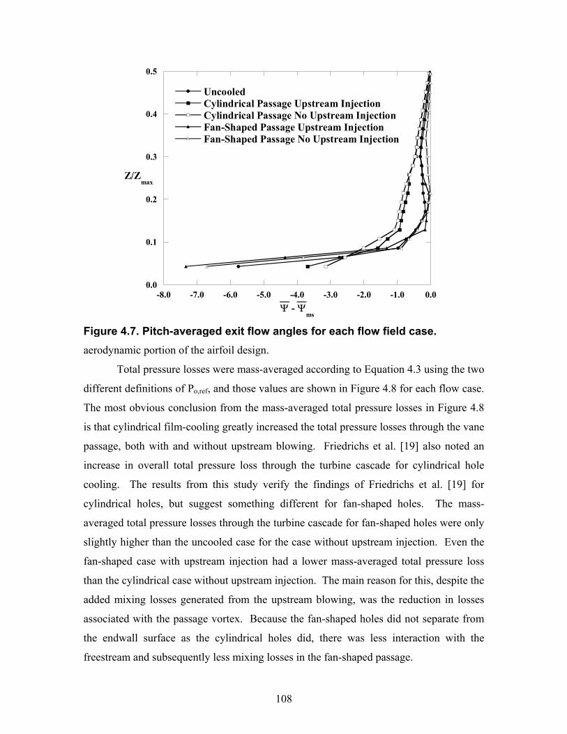
108

0.0

0.1

0.2

0.3

0.4

0.5

-8.0 -7.0 -6.0 -5.0 -4.0 -3.0 -2.0 -1.0 0.0

UncooledCylindrical Passage Upstream InjectionCylindrical Passage No Upstream InjectionFan-Shaped Passage Upstream InjectionFan-Shaped Passage No Upstream Injection

Ψ - Ψms

Z/Zmax

aerodynamic portion of the airfoil design.

Total pressure losses were mass-averaged according to Equation 4.3 using the two

different definitions of Po,ref, and those values are shown in Figure 4.8 for each flow case.

The most obvious conclusion from the mass-averaged total pressure losses in Figure 4.8

is that cylindrical film-cooling greatly increased the total pressure losses through the vane

passage, both with and without upstream blowing. Friedrichs et al. [19] also noted an

increase in overall total pressure loss through the turbine cascade for cylindrical hole

cooling. The results from this study verify the findings of Friedrichs et al. [19] for

cylindrical holes, but suggest something different for fan-shaped holes. The mass-

averaged total pressure losses through the turbine cascade for fan-shaped holes were only

slightly higher than the uncooled case for the case without upstream injection. Even the

fan-shaped case with upstream injection had a lower mass-averaged total pressure loss

than the cylindrical case without upstream injection. The main reason for this, despite the

added mixing losses generated from the upstream blowing, was the reduction in losses

associated with the passage vortex. Because the fan-shaped holes did not separate from

the endwall surface as the cylindrical holes did, there was less interaction with the

freestream and subsequently less mixing losses in the fan-shaped passage.

Figure 4.7. Pitch-averaged exit flow angles for each flow field case.

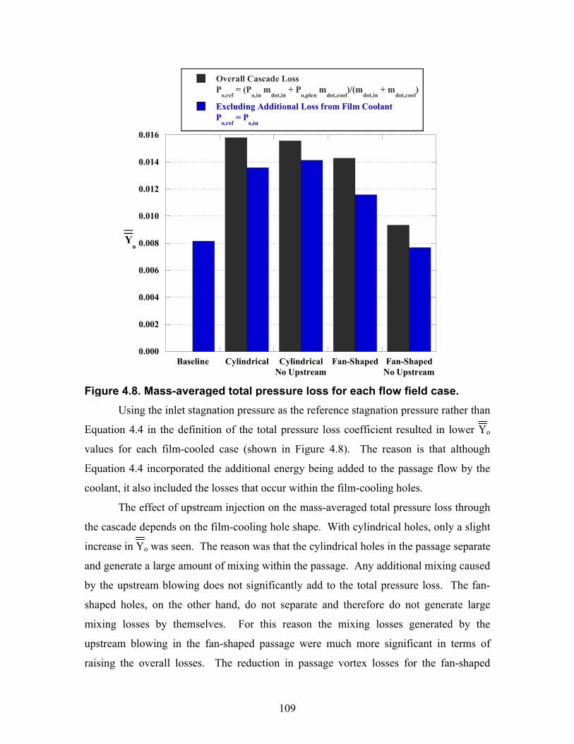
109

0.000

0.002

0.004

0.006

0.008

0.010

0.012

0.014

0.016

Baseline Cylindrical CylindricalNo Upstream

Fan-Shaped Fan-ShapedNo Upstream

Overall Cascade LossP

o,ref = (P

o,in m

dot,in + P

o,plen m

dot,cool)/(m

dot,in + m

dot,cool)

Excluding Additional Loss from Film CoolantP

o,ref = P

o,in

Yo

Using the inlet stagnation pressure as the reference stagnation pressure rather than

Equation 4.4 in the definition of the total pressure loss coefficient resulted in lower Yo

values for each film-cooled case (shown in Figure 4.8). The reason is that although

Equation 4.4 incorporated the additional energy being added to the passage flow by the

coolant, it also included the losses that occur within the film-cooling holes.

The effect of upstream injection on the mass-averaged total pressure loss through

the cascade depends on the film-cooling hole shape. With cylindrical holes, only a slight

increase in Yo was seen. The reason was that the cylindrical holes in the passage separate

and generate a large amount of mixing within the passage. Any additional mixing caused

by the upstream blowing does not significantly add to the total pressure loss. The fan-

shaped holes, on the other hand, do not separate and therefore do not generate large

mixing losses by themselves. For this reason the mixing losses generated by the

upstream blowing in the fan-shaped passage were much more significant in terms of

raising the overall losses. The reduction in passage vortex losses for the fan-shaped

Figure 4.8. Mass-averaged total pressure loss for each flow field case.

110

passage also contributed to the lower mass-averaged Yo values than for the cylindrical

passage. The study by Barigozzi et al. [18] showed little difference between the losses

generated for their fan-shaped passage versus their cylindrical passage. This however,

was attributed to the different number of holes between the the two passages. At the

same mass flow rate, fewer holes in the fan-shaped passage caused higher jet velocities,

leading to higher losses inside the hole than what would be seen if there had been a one-

to-one comparison.

Adiabatic Film-Cooling Effectiveness Measurements

Adiabatic film-cooling effectiveness measurements are shown in Figures 4.9a-f

for the cases with upstream coolant injection and in Figures 4.10a-f for the cases without

upstream injection. The cases shown in Figures 4.9a-f with upstream injection were

described in detail by Colban et al. [27] and are shown in this paper for comparison

purposes. It is particularly interesting that the upstream rows provided no immediate

cooling benefit to the endwall surface in any of the contours in Figure 4.9. All of the

coolant ejected from the upstream holes was completely separated from the surface, even

at the lowest tested MFRs due to the high surface angle.

In examining the differences between the cases without upstream coolant (shown

in Figure 4.10) and the cases with upstreamcoolant (shown in Figure 4.9), it is

immediately obvious that the overall levels of film-cooling effectiveness for the cases

without upstream injection were much lower. This is interesting given the fact that the

upstream holes offer no visible cooling benefit themselves, one would not expect levels

further downstream to be greatly reduced in the absence of upstream injection, although

certainly some of the improvement was probably due to a cooler near wall fluid from the

upstream blowing. Pressure ratios were matched between cases shown in Figures 4.9 and

4.10, so for instance, the passage film-cooling flow in Figures 4.9a and 4.10a are directly

comparable. In Figure 4.10a, the MFR is 0.36% for the passage film-cooling holes, while

in Figure 4.9a, the MFR was 0.36% for the passage film-cooling holes and 0.19% for the

upstream holes (making 0.55% total MFR for the case in Figure 4.9a). Considering the

fact that the amount of coolant issued from the film-cooling holes within the passage was

the same for the cases in both Figure 4.9 and Figure 4.10, it is suggested and confirmed

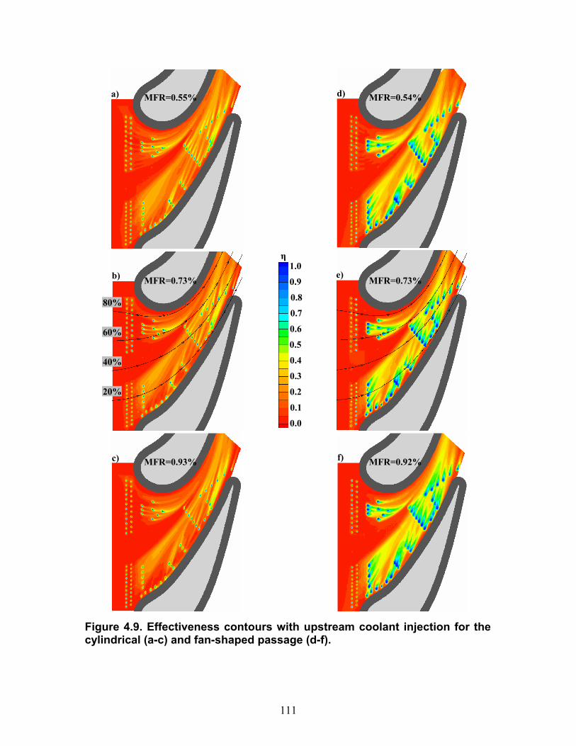
111

Figure 4.9. Effectiveness contours with upstream coolant injection for the cylindrical (a-c) and fan-shaped passage (d-f).

MFR=0.73%

e)

d) MFR=0.54%

a) MFR=0.55%

f) MFR=0.92%

c) MFR=0.93%

η1.0

0.9

0.8

0.7

0.6

0.5

0.4

0.3

0.2

0.1

0.0

MFR=0.73%

80%

b)

60%

40%

20%

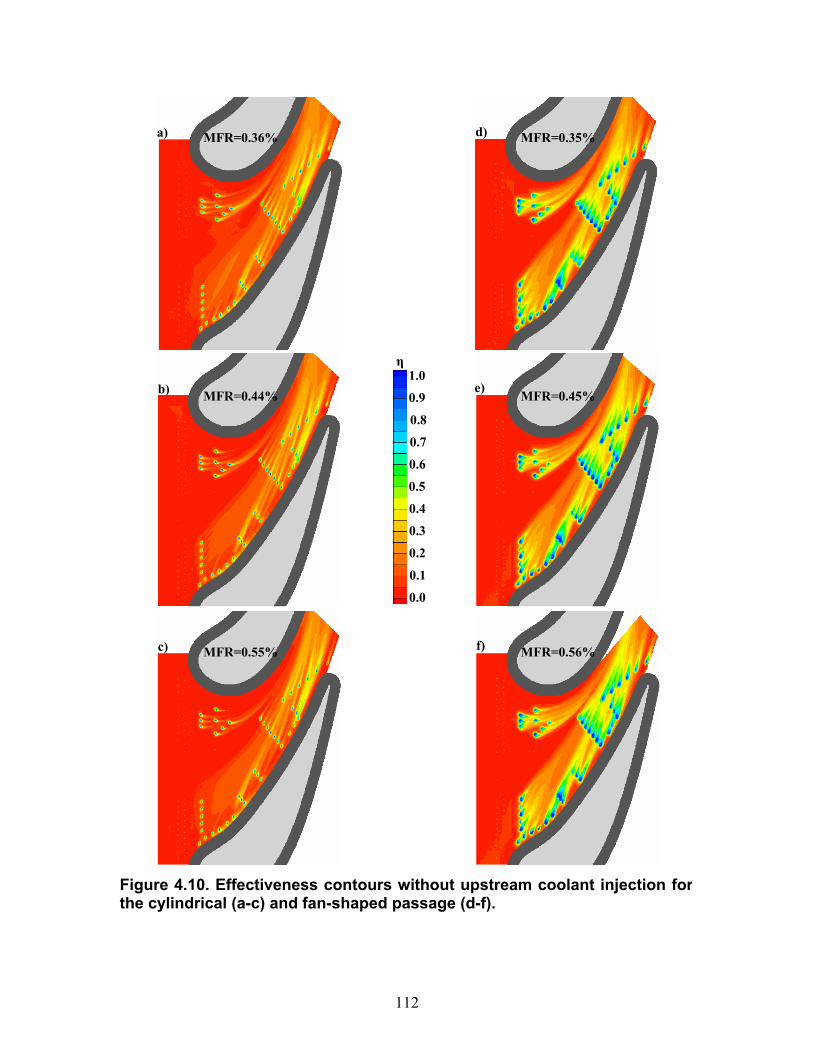
112

Figure 4.10. Effectiveness contours without upstream coolant injection forthe cylindrical (a-c) and fan-shaped passage (d-f).

MFR=0.45%

e)

d) MFR=0.35%

a) MFR=0.36%

f) MFR=0.56%

c) MFR=0.55%

η1.0

0.9

0.8

0.7

0.6

0.5

0.4

0.3

0.2

0.1

0.0

MFR=0.44%

b)

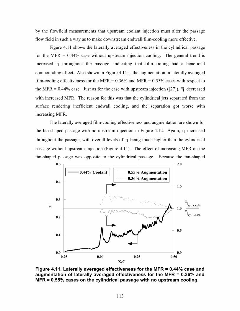
113

by the flowfield measurements that upstream coolant injection must alter the passage

flow field in such a way as to make downstream endwall film-cooling more effective.

Figure 4.11 shows the laterally averaged effectiveness in the cylindrical passage

for the MFR = 0.44% case without upstream injection cooling. The general trend is

increased η throughout the passage, indicating that film-cooling had a beneficial

compounding effect. Also shown in Figure 4.11 is the augmentation in laterally averaged

film-cooling effectiveness for the MFR = 0.36% and MFR = 0.55% cases with respect to

the MFR = 0.44% case. Just as for the case with upstream injection ([27]), η decreased

with increased MFR. The reason for this was that the cylindrical jets separated from the

surface rendering inefficient endwall cooling, and the separation got worse with

increasing MFR.

The laterally averaged film-cooling effectiveness and augmentation are shown for

the fan-shaped passage with no upstream injection in Figure 4.12. Again, η increased

throughout the passage, with overall levels of η being much higher than the cylindrical

passage without upstream injection (Figure 4.11). The effect of increasing MFR on the

fan-shaped passage was opposite to the cylindrical passage. Because the fan-shaped

0.0

0.1

0.2

0.3

0.4

0.5

0.0

0.5

1.0

1.5

2.0

-0.25 0.00 0.25 0.50

0.44% Coolant 0.55% Augmentation0.36% Augmentation

ηη

cyl, x.xx%

X/C

ηcyl, 0.44%

Figure 4.11. Laterally averaged effectiveness for the MFR = 0.44% case andaugmentation of laterally averaged effectiveness for the MFR = 0.36% and MFR = 0.55% cases on the cylindrical passage with no upstream cooling.

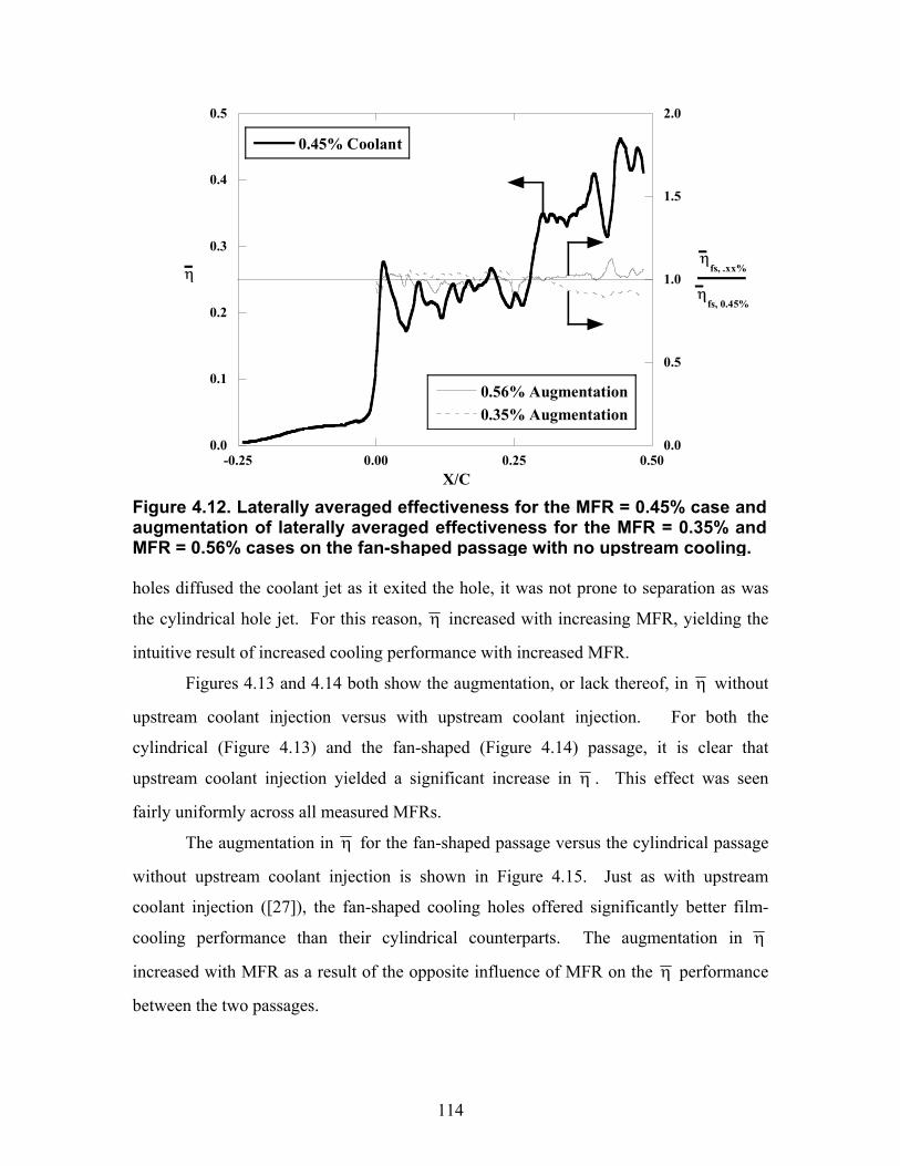
114

0.0

0.1

0.2

0.3

0.4

0.5

0.0

0.5

1.0

1.5

2.0

-0.25 0.00 0.25 0.50

0.45% Coolant

0.56% Augmentation0.35% Augmentation

ηη

fs, .xx%

X/C

ηfs, 0.45%

holes diffused the coolant jet as it exited the hole, it was not prone to separation as was

the cylindrical hole jet. For this reason, η increased with increasing MFR, yielding the

intuitive result of increased cooling performance with increased MFR.

Figures 4.13 and 4.14 both show the augmentation, or lack thereof, in η without

upstream coolant injection versus with upstream coolant injection. For both the

cylindrical (Figure 4.13) and the fan-shaped (Figure 4.14) passage, it is clear that

upstream coolant injection yielded a significant increase in η . This effect was seen

fairly uniformly across all measured MFRs.

The augmentation in η for the fan-shaped passage versus the cylindrical passage

without upstream coolant injection is shown in Figure 4.15. Just as with upstream

coolant injection ([27]), the fan-shaped cooling holes offered significantly better film-

cooling performance than their cylindrical counterparts. The augmentation in η

increased with MFR as a result of the opposite influence of MFR on the η performance

between the two passages.

Figure 4.12. Laterally averaged effectiveness for the MFR = 0.45% case andaugmentation of laterally averaged effectiveness for the MFR = 0.35% andMFR = 0.56% cases on the fan-shaped passage with no upstream cooling.

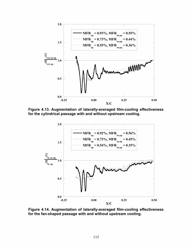
115

0.0

0.5

1.0

1.5

2.0

-0.25 0.00 0.25 0.50

MFRup

= 0.93%, MFRno,up

= 0.55%

MFRup

= 0.73%, MFRno,up

= 0.44%

MFRup

= 0.55%, MFRno,up

= 0.36%

X/C

ηcyl, no up

ηcyl, up

0.0

0.5

1.0

1.5

2.0

-0.25 0.00 0.25 0.50

MFRup

= 0.92%, MFRno,up

= 0.56%

MFRup

= 0.73%, MFRno,up

= 0.45%

MFRup

= 0.54%, MFRno,up

= 0.35%

X/C

ηfs, no up

ηfs, up

Figure 4.13. Augmentation of laterally-averaged film-cooling effectiveness for the cylindrical passage with and without upstream cooling.

Figure 4.14. Augmentation of laterally-averaged film-cooling effectiveness for the fan-shaped passage with and without upstream cooling.

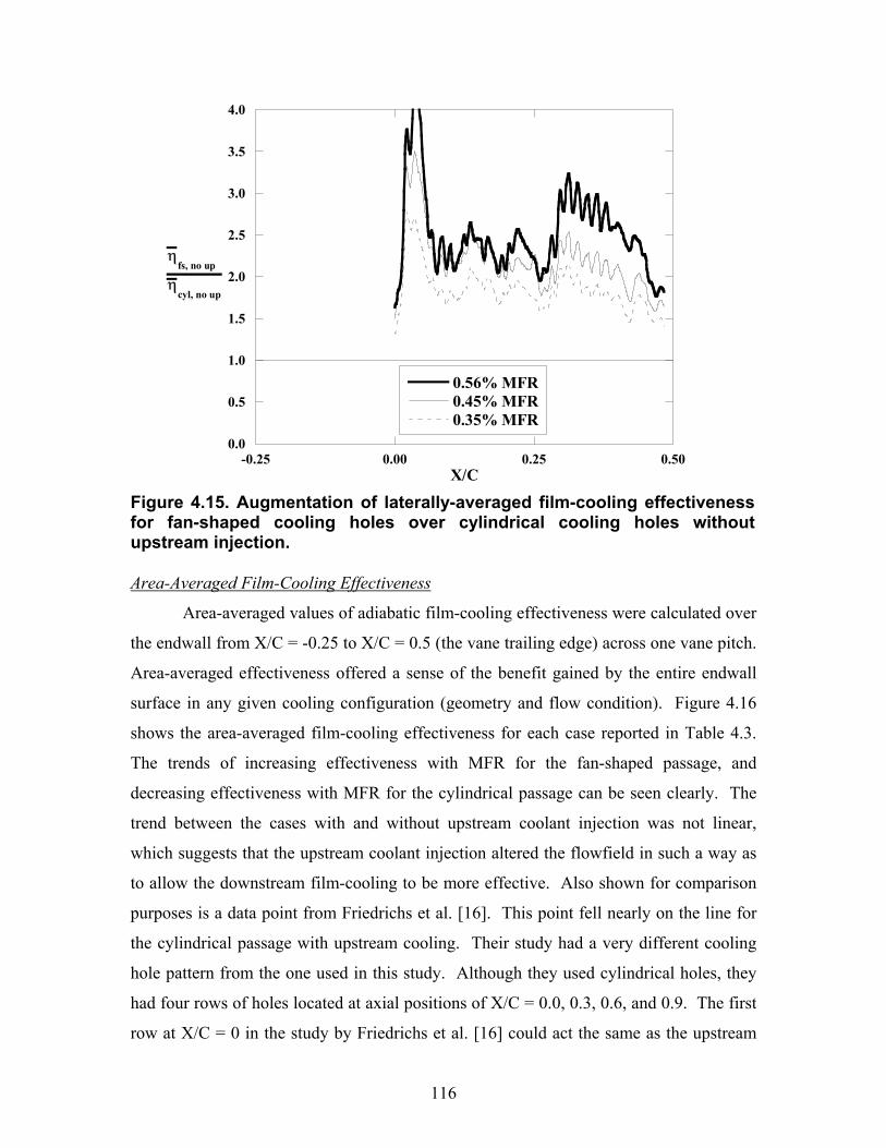
116

0.0

0.5

1.0

1.5

2.0

2.5

3.0

3.5

4.0

-0.25 0.00 0.25 0.50

0.56% MFR0.45% MFR0.35% MFR

X/C

ηfs, no up

ηcyl, no up

Area-Averaged Film-Cooling Effectiveness

Area-averaged values of adiabatic film-cooling effectiveness were calculated over

the endwall from X/C = -0.25 to X/C = 0.5 (the vane trailing edge) across one vane pitch.

Area-averaged effectiveness offered a sense of the benefit gained by the entire endwall

surface in any given cooling configuration (geometry and flow condition). Figure 4.16

shows the area-averaged film-cooling effectiveness for each case reported in Table 4.3.

The trends of increasing effectiveness with MFR for the fan-shaped passage, and

decreasing effectiveness with MFR for the cylindrical passage can be seen clearly. The

trend between the cases with and without upstream coolant injection was not linear,

which suggests that the upstream coolant injection altered the flowfield in such a way as

to allow the downstream film-cooling to be more effective. Also shown for comparison

purposes is a data point from Friedrichs et al. [16]. This point fell nearly on the line for

the cylindrical passage with upstream cooling. Their study had a very different cooling

hole pattern from the one used in this study. Although they used cylindrical holes, they

had four rows of holes located at axial positions of X/C = 0.0, 0.3, 0.6, and 0.9. The first

row at X/C = 0 in the study by Friedrichs et al. [16] could act the same as the upstream

Figure 4.15. Augmentation of laterally-averaged film-cooling effectiveness for fan-shaped cooling holes over cylindrical cooling holes withoutupstream injection.

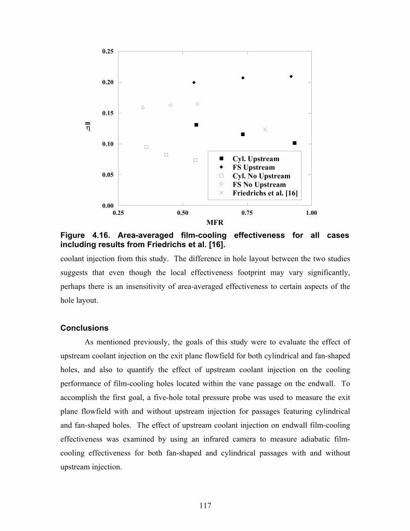
117

0.00

0.05

0.10

0.15

0.20

0.25

0.25 0.50 0.75 1.00

Cyl. UpstreamFS UpstreamCyl. No UpstreamFS No UpstreamFriedrichs et al. [16]

MFR

η

coolant injection from this study. The difference in hole layout between the two studies

suggests that even though the local effectiveness footprint may vary significantly,

perhaps there is an insensitivity of area-averaged effectiveness to certain aspects of the

hole layout.

Conclusions As mentioned previously, the goals of this study were to evaluate the effect of

upstream coolant injection on the exit plane flowfield for both cylindrical and fan-shaped

holes, and also to quantify the effect of upstream coolant injection on the cooling

performance of film-cooling holes located within the vane passage on the endwall. To

accomplish the first goal, a five-hole total pressure probe was used to measure the exit

plane flowfield with and without upstream injection for passages featuring cylindrical

and fan-shaped holes. The effect of upstream coolant injection on endwall film-cooling

effectiveness was examined by using an infrared camera to measure adiabatic film-

cooling effectiveness for both fan-shaped and cylindrical passages with and without

upstream injection.

Figure 4.16. Area-averaged film-cooling effectiveness for all cases including results from Friedrichs et al. [16].

118

The flowfield results indicated that cylindrical hole film-cooling increased the

total pressure losses generated by the passage vortex. Cylindrical hole film-cooling did

reduce the strength of the cross-passage flow, shifting the location of the passage vortex

towards the pressure side. The coolant separation in the cylindrical passage, which was

evident from the effectiveness contours, generated high mixing losses with the freestream.

The fan-shaped holes did not separate from the endwall, but the shear layer between the

coolant and the freestream still generated significant losses.

Both passages showed increased mixing and shear losses with upstream injection

relative to no upstream injection. Overall mass-averaged losses for the cylindrical

passage were much higher than the uncooled case because of the increase in passage

vortex losses and the added mixing losses. Overall mass-averaged losses for the fan-

shaped passage were nearly the same as for the uncooled case because the added shear

layer losses were counteracted by the reduction in losses generated by the passage vortex.

The flowfield results showed that fan-shaped holes generated less total pressure loss than

cylindrical holes, especially with no upstream blowing.

The adiabatic film-cooling effectiveness measurements showed that the coolant

from the upstream holes had little immediate cooling benefit to the endwall in the region

just downstream of the upstream injection, with the coolant separating entirely from the

endwall because of the high injection angle. However, further downstream in the passage,

effectiveness levels for the cases with upstream coolant were much higher, the reason

being that there was a large amount of coolant in the passage region from the upstream

injection. This coolant mixed with the freestream and lowered the temperature of the

near-wall fluid, resulting in higher effectiveness levels downstream in the passage. The

flow field results also indicated an influence on the passage flowfield by the upstream

coolant injection, which could have also contributed to the higher effectiveness levels.

The effect of increased MFR was to decrease η in the cylindrical passage because of jet

separation. In the fan-shaped passage the effect of increased MFR was to increase η

because the fan-shaped coolant jets stayed attached to the endwall surface.

The results of this study further illustrate the complexity of the film-cooling

design process. The addition of film-cooling holes on a turbine endwall has aerodynamic

consequences in addition to the thermal benefit that might be gained. Incorrect

119

placement of film-cooling holes can also prove wasteful. It is critical that engine

designers be aware of both the thermal and aerodynamic consequences of their film-

cooling hole designs. The results of this study are clear in their recommendation of fan-

shaped holes over cylindrical holes from both an aerodynamic and thermal perspective.

Fan-shaped holes showed lower total pressure losses, while at the same time providing

better film-cooling effectiveness than cylindrical holes.

Acknowledgments

The authors are grateful to Siemens Power Generation for their funding and


Nomenclature C true vane chord


I local momentum flux ratio, I = ρcoolUcool2/ρinUin

2

k thermal conductivity ⋅

m mass flow rate

M local blowing ratio, M = ρcoolUcool/ρinUin


P pressure, vane pitch

PS pressure side


S distance along the surface of the vane, measured from the vane stagnation

SS suction side

t hole breakout distance

T temperature

U velocity

Vn velocity normal to the streamwise direction, Vn = Vssin(Ψms – Ψ)

Vs streamwise velocity

Vz spanwise component of velocity, Vn = Vssin(Φ)


120

Y pitchwise coordinate

Yo total pressure loss coefficient, Yo = (Po,ref – Po,exit)/ (Po,ref – Ps,exit)

Z spanwise coordinate

Greek



η adiabatic film-cooling effectiveness, η = (T∞ – Tsurf)/(T∞ – Tcool)

ρ density



Φ pitch angle

Ψ yaw/flow turning angle

Subscripts

∞ freestream

base baseline case without any film-cooling

cool coolant

cyl cylindrical holes

exit exit plane

fs fan-shaped holes

in inlet condition

max maximum value

ms mid-span

no up no upstream injection

o total, uncooled effectiveness for conduction correction

plen plenum

ps pressure side

ref reference value

s static

ss suction side

121

surf surface

up upstream injection

Overbar

– lateral/pitchwise average

= area average or mass average

References [1] Morris A. W. H. and Hoare, R. G., "Secondary Loss Measurements in a Cascade

of Turbine Vanes with Meridional Wall Profiling," 75-WA/GT-13, 1975.

[2] Kercher, D. M., Film-Cooling Bibliography: 1940-2002: Private publication,

2003.

[3] Kercher, D. M., Film-Cooling Bibliography Addendum: 1999-2004: Private

publication, 2005.

[4] Goldstein, R. J., "Film Cooling," Advances in Heat Transfer, vol. 7, pp. 321-379,

1971.

[5] Bogard, D. G. and Thole, K. A., "Gas Turbine Film Cooling," to appear in the

AIAA Journal of Propulsion, 2006.

[6] Bunker, R. S., "A Review of Shaped Hole Turbine Film-Cooling Technology,"


[7] Blair, M. F., "An Experimental Study of Heat Transfer and Film Cooling on

Large-Scale Turbine Endwalls," ASME Journal of Heat Transfer, vol. 96, pp.

524-529, 1974.

[8] Granser, D. and Schulenberg, T., "Prediction and Measurement of Film Cooling

122

Effectiveness for a First Stage Turbine Vane Shroud," 90-GT-95, 1990.

[9] Colban, W., Thole, K. A., and Zess, G., "Combustor Turbine Interface Studies -

Part 1: Endwall Effectiveness Measurements," ASME Journal of Turbomachinery,

vol. 125, pp. 193-202, 2003.

[10] Knost, D. G. and Thole, K. A., "Computational Predictions of Endwall Film-

Cooling for a First Stage Vane," GT2003-38252, 2003.

[11] Knost, D. G. and Thole, K. A., "Adiabatic Effectiveness Measurements of

Endwall Film-Cooling for a First Stage Vane," ASME Journal of Turbomachinery,

vol. 127, pp. 297-305, 2005.

[12] Harasgama, S. P. and Burton, C. D., "Film Cooling Research on the Endwall of a

Turbine Nozzle Guide Vane in a Short Duration Annular Cascade: Part 1-

Experimental Technique and Results," ASME Journal of Turbomachinery, vol.

114, pp. 734-740, 1992.

[13] Nicklas, M., "Film-Cooled Turbine Endwall in a Transonic Flow Field: Part II -

Heat Transfer and Film-Cooling Effectiveness," 2001-GT-0146, 2001.

[14] Langston, L. S., Nice, M. L., and Hooper, R. M., "Three-Dimensional Flow

Within a Turbine Cascade Passage," ASME Journal of Engineering Power, vol.

99, pp. 21-28, 1977.

[15] Sieverding, C. H. and Wilputte, P., "Influence of Mach Number and Endwall

Cooling on Secondary Flows in a Straight Nozzle Cascade," ASME Journal of

Engineering for Gas Turbines and Power, vol. 103, pp. 257-264, 1981.

[16] Friedrichs, S., Hodson, H. P., and Dawes, W. N., "Distribution of Film-Cooling

Effectiveness on a Turbine Endwall Measured Using the Ammonia and Diazo

123

Technique," ASME Journal of Turbomachinery, vol. 118, pp. 613-621, 1995.

[17] Kost, F. and Nicklas, M., "Film-Cooled Turbine Endwall in a Transonic Flow

Field: Part I - Aerodynamic Measurements," 2001-GT-0145, 2001.

[18] Barigozzi, G., Benzoni, G., Franchini, G., and Perdichizzi, A., "Fan-Shaped Hole

Effects on the Aero-Thermal Performance of a Film Cooled Endwall," GT2005-

68544, 2005.

[19] Friedrichs, S., Hodson, H. P., and Dawes, W. N., "Aerodynamic Aspects of

Endwall Film-Cooling," ASME Journal of Turbomachinery, vol. 119, pp. 786-793,

1997.

[20] Oke, R. A., Burd, S. W., Simon, T. W., and Vahlberg, R., "Measurements in a

Turbine Cascade over a Contoured Endwall: Discrete Hole Injection of Bleed

Flow," 2000-GT-214, 2000.

[21] Zess, G. and Thole, K. A., "Computational Design and Experimental Evaluation

of Using a Leading Edge Fillet on a Gas Turbine Engine," ASME Journal of

Turbomachinery, vol. 124, pp. 167-175, 2002.

[22] Lethander, A. T. and Thole, K. A., "Optimizing the Vane-Endwall Junction to

Reduce Adiabatic Wall Temperatures in a Turbine Vane Passage," GT2003-

38940, 2003.

[23] Becz, S., Majewski, M. S., and Langston, L. S., "Leading Edge Modification

Effects on Turbine Cascade Endwall Loss," GT2003-38898, 2003.

[24] Mahmood, G. I., Gustafson, R., and Acharya, S., "Experimental Investigation of

Flow Structure and Nusselt Number in a Low-Speed Linear Blade Passage With

and Without Leading-Edge Fillets," ASME Journal of Heat Transfer, vol. 127, pp.

124

499-512, 2005.

[25] Zhang, L. J. and Jaiswal, R. S., "Turbine Nozzle Endwall Film Cooling Study

Using Pressure-Sensitive Paint," ASME Journal of Turbomachinery, vol. 123, pp.

730-738, 2001.

[26] Zhang, L. and Moon, H. K., "Turbine Nozzle Endwall Inlet Film Cooling - The

Effect of a Back-Facing Step," GT2003-38319, 2003.

[27] Colban, W., Thole, K. A., and Haendler, M., "A Comparison of Cylindrical and

Fan-Shaped Film-Cooling Holes on a Vane Endwall at Low and High Freestream

Turbulence Levels," GT2006-90021, 2006.

[28] Colban, W., Gratton, A., Thole, K. A., and Haendler, M., "Heat Transfer and

Film-Cooling Measurements on a Stator Vane with Fan-Shaped Cooling Holes,"

GT2005-68258, 2005.

[29] Colban, W., Thole, K. A., and Haendler, M., "Experimental and Computational

Comparisons of Fan-Shaped Film-Cooling on a Turbine Vane Surface,"

IMECE2005-79596, 2005.

[30] Moffat, R. J., "Describing the Uncertainties in Experimental Results,"


125

Summary of Findings and Recommendations for Future Work

This research focused on the performance of fan-shaped film-cooling holes on the

critical vane and endwall surfaces in a gas turbine vane. The first two papers dealt with

the vane results, while the last two papers dealt with the endwall results. The vane results

were split into single row measurements, discussed in the first paper, and multiple row

results and comparisons to computational predictions, which were discussed in the

second paper. A comparison of fan-shaped and cylindrical holes on the endwall at both

high and low freestream turbulence was given in the third paper. The fourth and final

paper gave a summary of the effect of upstream injection on the endwall for both hole

geometries, and examined the aerodynamic performance of both hole shapes for the

endwall.

The first paper described in detail the high-resolution single-row adiabatic film-

cooling effectiveness measurements on the vane with fan-shaped holes. A number of

critical regions were identified, including the first pressure side row and the first suction

side row. The first pressure side row was located in a region of concave curvature. The

coolant partially separated before reattaching further along the surface. The reattachment

acted as an impingement, spreading the coolant laterally and raising effectiveness levels.

The first suction side row was located in a region of convex curvature. The coolant from

this row separated from the surface because of the strong curvature, with lower blowing

ratios offering better cooling for this region. Showerhead measurements also revealed

significant lift-off with higher blowing ratios, resulting from the high surface angles of

the showerhead holes.

The second paper was meant to be a parallel paper to the first, offering film-

cooling measurements on the vane with multiple rows of cooling holes. Overall,

effectiveness levels increased with blowing ratio for the multiple row configurations, as

compared to a reduction in cooling effectiveness with blowing ratio for most of the single

rows of holes as reported in the first paper. The CFD predictions offered mixed results,

with the RNG-kε model coming closer to the averaged film-cooling effectiveness levels,

while the v2-f model gave a better prediction of the separation at the leading edge. The

v2-f model, however, had trouble predicting the lateral spreading of the coolant, which

126

resulted in an over-prediction of film-cooling effectiveness.

The third paper gave a direct comparison of fan-shaped holes to cylindrical holes

on the endwall surface with high and low freestream turbulence. The major finding from

that study was to show that fan-shaped holes offered an increase in film-cooling

effectiveness of 75% percent over cylindrical holes at low freestream turbulence. The

reason was that the fan-shaped holes spread out more in the lateral direction and stayed

attached to the surface, while the cylindrical cooling holes showed little lateral spreading

and separated off of the surface. The effect of high freestream turbulence was to reduce

the effectiveness by 6% in the fan-shaped passage and to change the dependency of

effectiveness on flow rate for the cylindrical passage.

The fourth and final paper examined the effect of upstream coolant injection on

the film-cooling performance for both cooling hole geometries on the endwall. The

aerodynamic performance of each cooling hole shape on the endwall was also

investigated using a five-hole probe to measure total pressure losses through the passage.

While upstream coolant injection offered little immediate cooling benefit in the near-hole

region, it saturated the near-wall region with coolant and increased effectiveness levels in

the endwall region downstream. Flowfield measurements showed that the highest losses

in the exit plane were generated by the passage vortex. Cylindrical film-cooling tended

to reduce the strength of the cross-passage flow and increase the strength of the losses

generated by the passage vortex. High losses resulted from separated film-cooling

mixing with the freestream in the cylindrical passage. For the fan-shaped passage, the

coolant remained near the wall, and the shear layer between the coolant and freestream

generated additional losses. For both passages, upstream coolant injection generated

additional mixing losses.

One other major achievement of this work was related to the data processing. A

unique transformation routine was developed to unwrap distorted surface images into

rectangular coordinates. The transformation routine was necessary to yield quantifiable

results on the vane surface. The unique approach taken to measure film-cooling

effectiveness from below the test section allowed previously unobtainable high resolution

measurements on the vane surface.

127

Recommendations for Future Work Although this study offered a comprehensive examination of fan-shaped film-

cooling in the turbine vane passage, there is still a significant amount of work that could

be done to better understand the behavior of film-cooling in the extremely complex

region. There are a number or areas in which additional research could be performed,

including vane heat transfer with film-cooling.

In a study that paralleled this research, Gratton [1] measured heat transfer

coefficients on the vane surface for the same airfoil shape. Although a great amount was

learned from that work, the original desire was to also measure heat transfer coefficients

with vane film-cooling. The measurement of surface heat transfer coefficients with film-

cooling should be performed.

The computational predictions shown in paper 2 of this study were not as close as

hoped for. Obviously there is significant room for improvement in the area of full-scale

multiple-row film-cooling predictions. Many current computational film-cooling studies

involve the modeling of only a single hole, or very few holes. Although the capability

exists to accurately model those more simple situations, often accurate solutions require

time-dependent models with resolution down to y+ < 1. Obviously those types of

computations cannot be done yet for the full vane, although because of the complexity of

film-cooling flow, perhaps time-dependent calculations will be required for the multiple-

row configuration as well to obtain more accurate predictions.

For the endwall measurements, although a lot of information can be extracted

from surface measurements, there is still the need for field measurements, both thermal

and flowfield. It is possible to determine whether or not a cooling jet separates from the

surface from surface measurements of adiabatic film-cooling effectiveness. However, the

surface measurements offer no indication of how the separated film migrates through the

passage. Also, more flowfield measurements within the passage would provide a glimpse

of the secondary flow development through the passage. There is still much to learn as to

how the upstream injection affects the passage flow development.

One other investigation that would be particularly interesting would be a

combined vane and endwall film-cooling study. During engine operation both the vane

and endwall surfaces are film-cooled. In the presence of secondary flows, which sweep

128

flow down the vane pressure side surface and onto the endwall, perhaps some of the vane

film-cooling near the vane-endwall junction has some cooling benefit for the endwall

surface. The current facility was constructed with this particular investigation in mind for

future researchers.

References [1] Gratton, A., 2004, “Measurements and Predictions of Heat Transfer for a First

Vane Design,” Master’s Thesis, Virginia Polytechnic and State University.

129

Appendix A: Design and Construction of Experimental Facilities

Vane Construction There were many considerations that went into designing the film-cooling vane,

some of which were hole layout, plenum division, material selection, manufacturing

technique, and instrumentation. This section describes the development of the film-

cooling vane design in detail, describing each of the considerations listed above. The

first step in the design process was determined by the exit width from the combustor

simulator test section in the VTExCCL wind tunnel. In order to have two passages with a

center film-cooled vane, the maximum possible scaling parameter was 3X from the

airfoil geometry given by Siemens.

The design of the vane was in large part dictated by the sponsor, and a

considerable effort was made to maintain the integrity of the engine design in the large-

scale wind tunnel facility. The hole geometry, the surface locations on the vane of each

row of holes, the wall thickness, and the relative hole spacing were all taken from the

Siemens engine design and applied to the 3X scale experimental vane. The actual

Siemens vane is shown in Figure A.1a, alongside the vane design for this study at 3X

scale (Figure A.1b). The airfoil profile shape is identical for both designs, as well as the

hole placement of each row that was modeled.

Slight adjustments were made to the hole spacing in the spanwise direction in

order to obtain a periodic hole pattern every 6 cm (11% span). The pattern periodicity

was vital to accurate and meaningful lateral averaging, as well as later computational

fluid dynamics (CFD) simulations. Figure A.2 shows the hole pattern for the Siemens

engine design in red, with the current 3X periodic hole pattern outlined in black showing

both patterns being very similar. The exact hole spacing values are shown in Table A.1

for both the engine and experimental designs.

It was desired to match as closely as possible the blowing ratios at engine

conditions for the experimental vane. Blowing ratios at engine conditions for each row

of holes were calculated from the information provided by Siemens. To correctly match

the engine blowing ratios, the vane interior was divided into plenums. Because the

130

exterior flow conditions and pressure ratios were not the same as the engine, and there

were no impingement plates in the 3X scale vane, the plenum division had to be

determined by matching predicted blowing ratios at low speed conditions to the engine

blowing ratios.

The plenum supply pressure needed to achieve the correct blowing ratio was

determined for each row of holes for the film-cooling vane. Plenum locations were

Figure A.2 The hole layout for the Siemens engine vane is shown in red,while the current 3X hole layout is shown in black. The current design isperiodic every 11% span (inlet span).

PA PCPB PD

SA SC SB SD6 cm

Figure A.1 Film-cooling vane layouts for (a) the Siemens engine design and(b) the current 3X vane design.

PA

PB

PC

PD

SA SC

SB

SD

HA-E

PA

PB

PC

PD

SA

SC

SB

SD

HA-E

a) Siemens Design b) Current 3X Design

131

Hole Location Siemens Current t/P t/P

PA 0.54 0.54 PB 0.45 0.41 PC 0.45 0.41 PD 0.27 0.27 HA 0.21 0.22 HB 0.21 0.22 HC 0.21 0.22 HD 0.21 0.22 HE 0.21 0.22 SA 0.34 0.41 SB 0.45 0.41 SC 0.45 0.41 SD 0.80 0.81

decided on by grouping rows together based on their location on the vane and their

calculated necessary supply pressures. Figure A.1b shows the four plenum divisions that

were chosen for the interior of the experimental vane. A comparison of the engine local

blowing ratios with the predicted local blowing ratios based on the plenum division in the

experimental vane is shown in Table A.2. With the plenum division that was chosen, the

predicted blowing ratios compared well to those at engine conditions. The four

independent plenums required four independently controlled inlet flow feeds.

A number of different methods were considered from which to construct the film-

cooling vane. The three requirements for the test vane were the following: (1) a material

with a low thermal conductivity to minimize lateral and radial conduction losses, (2) a

material that would be strong enough such that it would support the interior plenum

pressure, and (3) a material that would maintain the geometric integrity of the hole

shaped after the manufacturing process. The final design was chosen based on the results

of a conduction loss analysis, the manufacturing difficulty, and the cost.

Hole Location Siemens Predicted M M

PA 2.1 1.9 PB 2.8 2.9 PC 3.9 3.8 PD 5.9 5.9 SA 3.0 3.0 SB 1.8 1.8 SC 1.5 1.5 SD 1.2 1.1

Table A.2 Comparison Between Engine Blowing Ratios to Predicted Values

Table A.1 Hole Spacing Parameter for Engine Vane and Design Vane

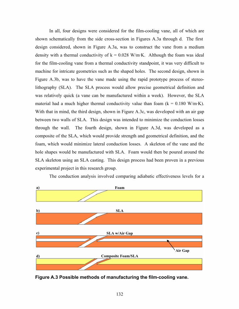
132

In all, four designs were considered for the film-cooling vane, all of which are

shown schematically from the side cross-section in Figures A.3a through d. The first

design considered, shown in Figure A.3a, was to construct the vane from a medium

density with a thermal conductivity of k = 0.028 W/m·K. Although the foam was ideal

for the film-cooling vane from a thermal conductivity standpoint, it was very difficult to

machine for intricate geometries such as the shaped holes. The second design, shown in

Figure A.3b, was to have the vane made using the rapid prototype process of stereo-

lithography (SLA). The SLA process would allow precise geometrical definition and

was relatively quick (a vane can be manufactured within a week). However, the SLA

material had a much higher thermal conductivity value than foam (k = 0.180 W/m·K).

With that in mind, the third design, shown in Figure A.3c, was developed with an air gap

between two walls of SLA. This design was intended to minimize the conduction losses

through the wall. The fourth design, shown in Figure A.3d, was developed as a

composite of the SLA, which would provide strength and geometrical definition, and the

foam, which would minimize lateral conduction losses. A skeleton of the vane and the

hole shapes would be manufactured with SLA. Foam would then be poured around the

SLA skeleton using an SLA casting. This design process had been proven in a previous

experimental project in this research group.

The conduction analysis involved comparing adiabatic effectiveness levels for a

Air Gap

Foam

SLA

SLA w/Air Gap

Composite Foam/SLA

a)

b)

c)

d)

Figure A.3 Possible methods of manufacturing the film-cooling vane.

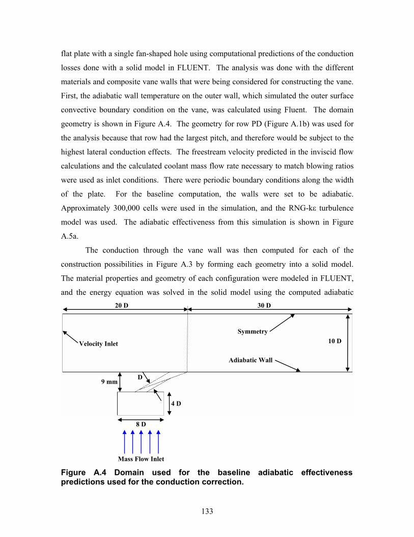
133

flat plate with a single fan-shaped hole using computational predictions of the conduction

losses done with a solid model in FLUENT. The analysis was done with the different

materials and composite vane walls that were being considered for constructing the vane.

First, the adiabatic wall temperature on the outer wall, which simulated the outer surface

convective boundary condition on the vane, was calculated using Fluent. The domain

geometry is shown in Figure A.4. The geometry for row PD (Figure A.1b) was used for

the analysis because that row had the largest pitch, and therefore would be subject to the

highest lateral conduction effects. The freestream velocity predicted in the inviscid flow

calculations and the calculated coolant mass flow rate necessary to match blowing ratios

were used as inlet conditions. There were periodic boundary conditions along the width

of the plate. For the baseline computation, the walls were set to be adiabatic.

Approximately 300,000 cells were used in the simulation, and the RNG-kε turbulence

model was used. The adiabatic effectiveness from this simulation is shown in Figure

A.5a.

The conduction through the vane wall was then computed for each of the

construction possibilities in Figure A.3 by forming each geometry into a solid model.

The material properties and geometry of each configuration were modeled in FLUENT,

and the energy equation was solved in the solid model using the computed adiabatic

10 D

8 D

4 D

30 D 20 D

D

Adiabatic Wall

Mass Flow Inlet

Velocity Inlet

Symmetry

9 mm

Figure A.4 Domain used for the baseline adiabatic effectivenesspredictions used for the conduction correction.

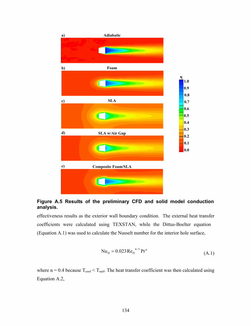
134

effectiveness results as the exterior wall boundary condition. The external heat transfer

coefficients were calculated using TEXSTAN, while the Dittus-Boelter equation

(Equation A.1) was used to calculate the Nusselt number for the interior hole surface,

n5/4

DD PrRe023.0Nu = (A.1)

where n = 0.4 because Tcool < Tsurf. The heat transfer coefficient was then calculated using

Equation A.2,

Adiabatic

Foam

SLA

Composite Foam/SLA

SLA w/Air Gap

η 1.0 0.9

0.8 0.7 0.6

0.5 0.4 0.3 0.2 0.1

0.0

a)

b)

c)

d)

e)

Figure A.5 Results of the preliminary CFD and solid model conductionanalysis.

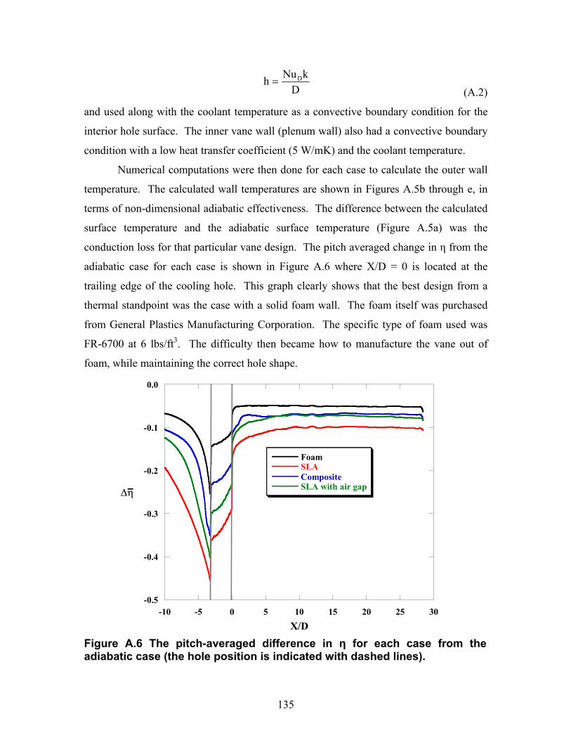
135

DkNuh D=

(A.2)

and used along with the coolant temperature as a convective boundary condition for the

interior hole surface. The inner vane wall (plenum wall) also had a convective boundary

condition with a low heat transfer coefficient (5 W/mK) and the coolant temperature.

Numerical computations were then done for each case to calculate the outer wall

temperature. The calculated wall temperatures are shown in Figures A.5b through e, in

terms of non-dimensional adiabatic effectiveness. The difference between the calculated

surface temperature and the adiabatic surface temperature (Figure A.5a) was the

conduction loss for that particular vane design. The pitch averaged change in η from the

adiabatic case for each case is shown in Figure A.6 where X/D = 0 is located at the

trailing edge of the cooling hole. This graph clearly shows that the best design from a

thermal standpoint was the case with a solid foam wall. The foam itself was purchased

from General Plastics Manufacturing Corporation. The specific type of foam used was

FR-6700 at 6 lbs/ft3. The difficulty then became how to manufacture the vane out of

foam, while maintaining the correct hole shape.

-0.5

-0.4

-0.3

-0.2

-0.1

0.0

-10 -5 0 5 10 15 20 25 30

FoamSLACompositeSLA with air gap∆η

X/D

Figure A.6 The pitch-averaged difference in η for each case from the adiabatic case (the hole position is indicated with dashed lines).

136

The construction of the vane from medium density foam was a two part process.

First, the airfoil profile, complete with the contoured endwall contraction, was machined

using a computer numerically controlled (CNC) mill. Next, the airfoil shell was sent to a

5-axis waterjet company, where the film-cooling holes were manufactured. The 5-axis

waterjet allowed a high geometrical integrity for the fan-shaped holes, although there

were some inconsistencies in hole diameter and hole shape and these irregularities were

accounted for (see Appendix D).

Finally, the interior and exterior of the vane were instrumented with numerous

thermocouples and pressure taps. Type E thermocouples were placed flush with the vane

surface in order to accurately calibrate the infrared (IR) images. Thermocouples were

also located in each plenum to measure the coolant temperature during tests. Static

pressure taps were located around the vane surface to measure the flow distribution

around the vane prior to testing. Total pressure taps were also located in each plenum to

measure pressure ratios and set blowing ratios during tests.

Endwall Construction Construction of the endwall was very similar in approach and technique to the

vane design. The Siemens endwall film-cooling pattern for the engine is shown in Figure

A.7a. The holes that were chosen to be incorporated into the experimental endwall are

highlighted in Figure A.7a. The engine endwall design featured separate plenums for

different groups of holes and also included an impingement plate. These features were

not included in the 3X scale design, as all of the holes were fed from a single plenum.

The 3X scale endwall design is shown in Figure A.7b, and featured two passages, one

with cylindrical cooling holes in the passage and the other with fan-shaped cooling holes

in the passage. For both passages, a double row of staggered 60º cylindrical holes were

located upstream of the passage.

Also, the manufacturing fillet was included in the experimental model. The fillet

was an elliptical design, and extended vertically to a height of 12D and radially to a

distance of 10D. The fillet was made by SLA and was secured to the vane-endwall

junction circumferentially around the base of the vane.

A single supply plenum was located beneath the test section, which supplied

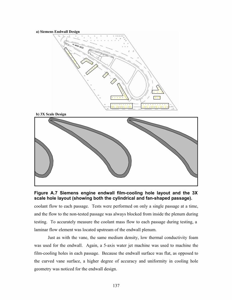
137

coolant flow to each passage. Tests were performed on only a single passage at a time,

and the flow to the non-tested passage was always blocked from inside the plenum during

testing. To accurately measure the coolant mass flow to each passage during testing, a

laminar flow element was located upstream of the endwall plenum.

Just as with the vane, the same medium density, low thermal conductivity foam

was used for the endwall. Again, a 5-axis water jet machine was used to machine the

film-cooling holes in each passage. Because the endwall surface was flat, as opposed to

the curved vane surface, a higher degree of accuracy and uniformity in cooling hole

geometry was noticed for the endwall design.

Figure A.7 Siemens engine endwall film-cooling hole layout and the 3X scale hole layout (showing both the cylindrical and fan-shaped passage).

a) Siemens Endwall Design

b) 3X Scale Design

138

Prior to testing, the endwall surface and plenum interior were instrumented with

thermocouples and pressure taps to record pertinent temperature and pressure data during

testing. Nine type E thermocouples were placed flush with the endwall surface in each

passage with which to calibrate the IR images. Thermocouples were also placed within

the plenum to monitor coolant temperatures during the endwall tests. Pressure taps were

placed upstream of the vane passage on the endwall to measure the upstream static

pressure on the endwall, and provide a reference with which to calculate local blowing

ratios using the static pressure distribution on the endwall obtained from CFD for the

uncooled case. Pressure taps were also located within the plenum to measure the

pressure ratio within the plenum.

Nomenclature D film-cooling hole diameter

h heat transfer coefficient, h = NuDK/D


M local blowing ratio, M = ρcoolUcool/ρinUin

n power for the Dittus-Boelter equation, n = 0.4 for Tcool < Tsurf

Nu Nusselt number, for this study, NuD = 0.023ReD4/5Prn (n = 0.4, Dittus-Boelter)

P spacing between adjacent holes

Pr Prandtl number


T temperature

U velocity


Greek


ρ density

Subscripts

∞ freestream

139

cool coolant

D diameter

in inlet condition

surf surface

Overbar

– lateral/pitchwise average

140

Appendix B: Data Analysis

Adiabatic Film-Cooling Effectiveness Measurements To obtain any quantitative results for the adiabatic effectiveness on the vane

surface, the infrared (IR) images needed to undergo a rigorous post-processing analysis

including the following: a three-dimensional surface transformation, a calibration to

ensure accurate temperatures on the surface, and a one-dimensional conduction

correction to account for conduction losses through the vane wall. The transformation

process is illustrated in Figure B.1, showing the initial raw IR image, and the subsequent

transformation, calibration, and conduction correction. The following three sub-sections

describe each of these tasks in detail.

Three-Dimensional Surface Transformation

The test section for the vane surface measurements is shown in Figure B.2.

Because of the adjacent vanes on either side of the center vane, it was not possible to

place the IR camera perpendicular to the vane surface. For this reason, it was chosen to

locate the IR camera underneath the test section as shown in Figure B.3. Images were

taken at approximately 45º to the vane surface. There were ten different locations that

were required to get a complete contour map of the vane surface. Each image station was

constructed such that the IR camera could be removed and then replaced in the exact

same spot, resulting in a repeatable image location. Repeatable image locations greatly

simplified the data reduction process.

Not only were the images taken at a 45º angle with respect to the surface, but the

surface was also highly curved. The curvature and picture distortion required a

transformation procedure that would transform the IR image into rectangular coordinates.

A fully interactive image transformation program was written in MATLAB that allowed

transformation of a uniform grid that was distorted in some way as to look non-uniform

in the image. In addition, another interactive program was written in MATLAB to apply

the same image transformation to an image taken at the same location, for instance a

picture taken during testing.

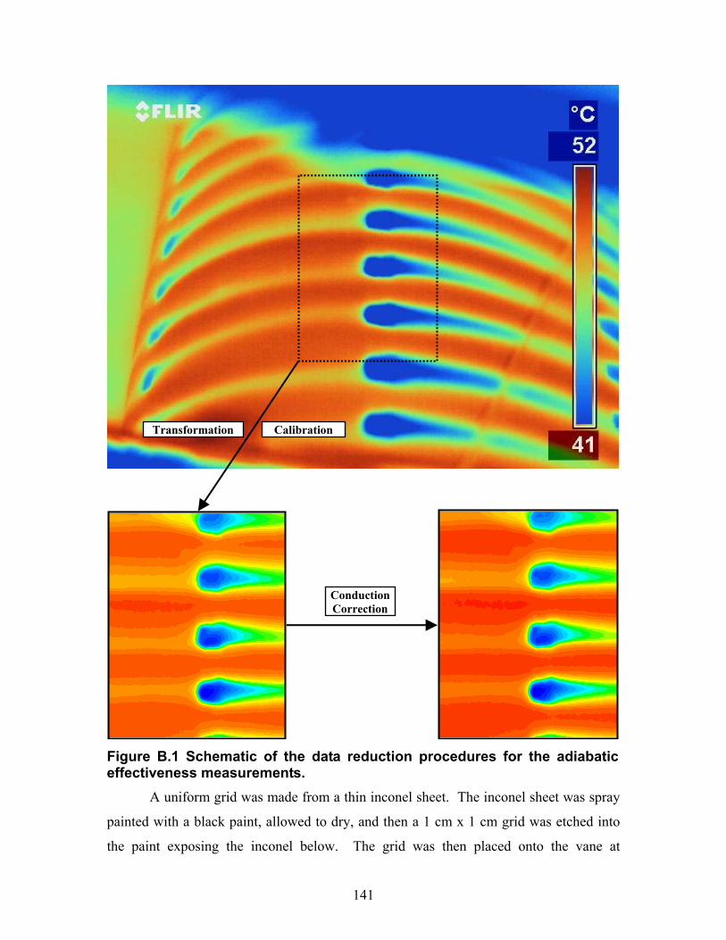
141

A uniform grid was made from a thin inconel sheet. The inconel sheet was spray

painted with a black paint, allowed to dry, and then a 1 cm x 1 cm grid was etched into

the paint exposing the inconel below. The grid was then placed onto the vane at

Calibration Transformation

ConductionCorrection

Figure B.1 Schematic of the data reduction procedures for the adiabaticeffectiveness measurements.

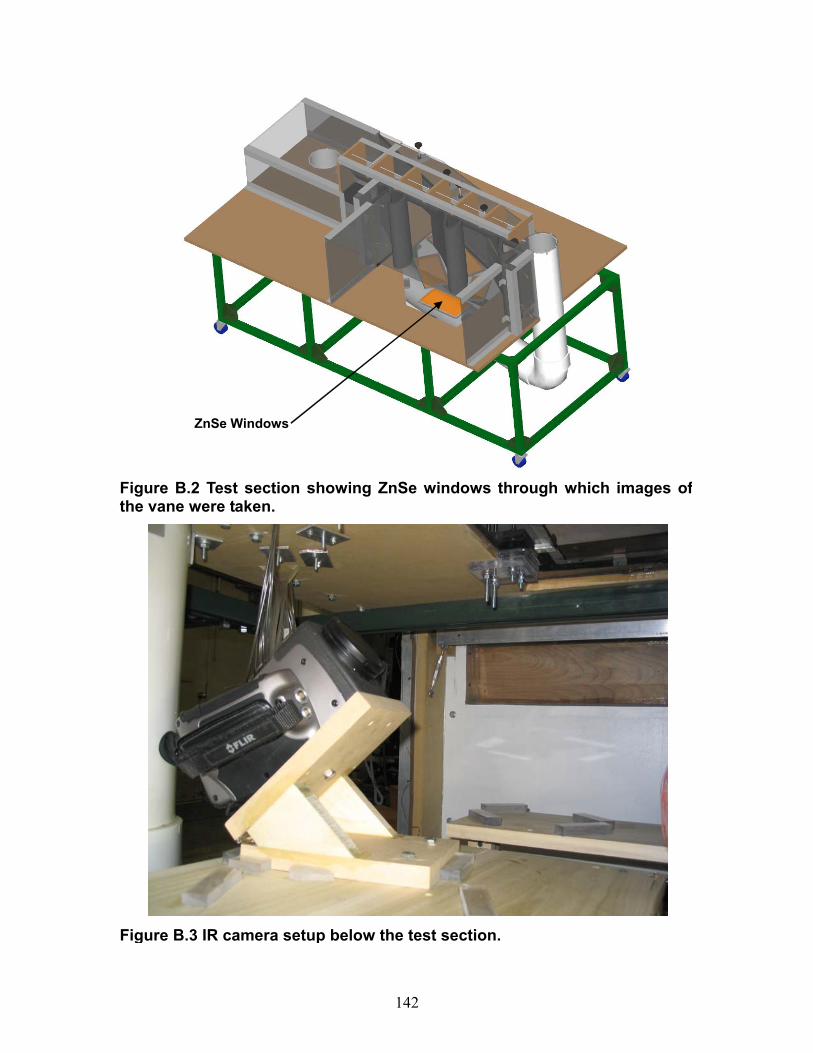
142

ZnSe Windows

Figure B.3 IR camera setup below the test section.

Figure B.2 Test section showing ZnSe windows through which images ofthe vane were taken.

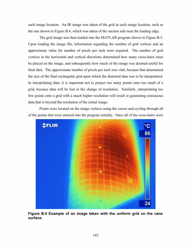
143

each image location. An IR image was taken of the grid at each image location, such as

the one shown in Figure B.4, which was taken of the suction side near the leading edge.

The grid image was then loaded into the MATLAB program shown in Figure B.5.

Upon loading the image file, information regarding the number of grid vertices and an

approximate value for number of pixels per inch were required. The number of grid

vertices in the horizontal and vertical directions determined how many cross-hairs must

be placed on the image, and subsequently how much of the image was deemed useful for

final data. The approximate number of pixels per inch was vital, because that determined

the size of the final rectangular grid upon which the distorted data was to be interpolated.

In interpolating data, it is important not to project too many points onto too small of a

grid, because data will be lost in the change of resolution. Similarly, interpolating too

few points onto a grid with a much higher resolution will result in generating extraneous

data that is beyond the resolution of the initial image.

Points were located on the image vertices using the cursor and cycling through all

of the points that were entered into the program initially. Once all of the cross-hairs were

Figure B.4 Example of an image taken with the uniform grid on the vane surface.

144

Pixel Locations on Grid Image Clipped Image

Unwrapped Image Transformation Selection

located correctly on a grid vertex, the image was cropped based on the minimum and

maximum extents of the cross-hairs placed on the grid image. The clipped image is

shown in the upper right-hand corner of Figure B.5. The reason the image was cropped is

that the following transformation was valid only in the region where the cross-hairs were

located, so it wasn’t necessary to apply the transformation to the entire image.

Several options were available for the transformation procedure. The

transformation can be understood by imaging the distorted grid image to be placed on the

surface of a balloon. The rectangular grid would then be obtained by stretching the

material in such a way to make the grid image appear rectangular. The different

transformation techniques were essentially different ways of stretching the image. The

3rd and 4th order polynomial and piecewise linear transformations were used for the vane.

Figure B.5 Grid image transformation program.

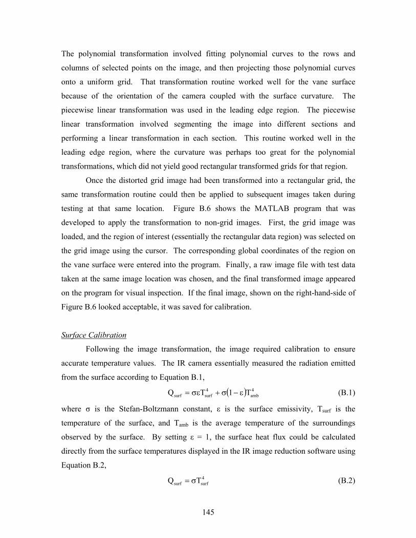
145

The polynomial transformation involved fitting polynomial curves to the rows and

columns of selected points on the image, and then projecting those polynomial curves

onto a uniform grid. That transformation routine worked well for the vane surface

because of the orientation of the camera coupled with the surface curvature. The

piecewise linear transformation was used in the leading edge region. The piecewise

linear transformation involved segmenting the image into different sections and

performing a linear transformation in each section. This routine worked well in the

leading edge region, where the curvature was perhaps too great for the polynomial

transformations, which did not yield good rectangular transformed grids for that region.

Once the distorted grid image had been transformed into a rectangular grid, the

same transformation routine could then be applied to subsequent images taken during

testing at that same location. Figure B.6 shows the MATLAB program that was

developed to apply the transformation to non-grid images. First, the grid image was

loaded, and the region of interest (essentially the rectangular data region) was selected on

the grid image using the cursor. The corresponding global coordinates of the region on

the vane surface were entered into the program. Finally, a raw image file with test data

taken at the same image location was chosen, and the final transformed image appeared

on the program for visual inspection. If the final image, shown on the right-hand-side of

Figure B.6 looked acceptable, it was saved for calibration.

Surface Calibration

Following the image transformation, the image required calibration to ensure

accurate temperature values. The IR camera essentially measured the radiation emitted

from the surface according to Equation B.1,

( ) 4amb

4surfsurf T1TQ ε−σ+σε= (B.1)

where σ is the Stefan-Boltzmann constant, ε is the surface emissivity, Tsurf is the

temperature of the surface, and Tamb is the average temperature of the surroundings

observed by the surface. By setting ε = 1, the surface heat flux could be calculated

directly from the surface temperatures displayed in the IR image reduction software using

Equation B.2, 4surfsurf TQ σ= (B.2)

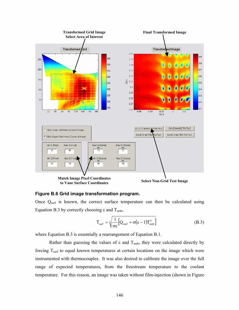
146

Once Qsurf is known, the correct surface temperature can then be calculated using

Equation B.3 by correctly choosing ε and Tamb,

( )[ ]4 4ambsurfsurf T1Q1T −εσ+

σε= (B.3)

where Equation B.3 is essentially a rearrangement of Equation B.1.

Rather than guessing the values of ε and Tamb, they were calculated directly by

forcing Tsurf to equal known temperatures at certain locations on the image which were

instrumented with thermocouples. It was also desired to calibrate the image over the full

range of expected temperatures, from the freestream temperature to the coolant

temperature. For this reason, an image was taken without film-injection (shown in Figure

Transformed Grid Image Select Area of Interest

Final Transformed Image

Select Non-Grid Test Image Match Image Pixel Coordinates

to Vane Surface Coordinates

Figure B.6 Grid image transformation program.

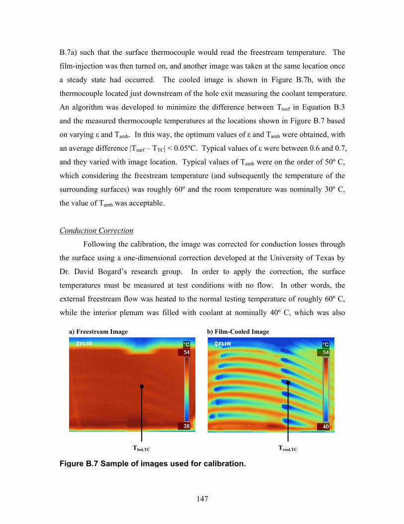
147

B.7a) such that the surface thermocouple would read the freestream temperature. The

film-injection was then turned on, and another image was taken at the same location once

a steady state had occurred. The cooled image is shown in Figure B.7b, with the

thermocouple located just downstream of the hole exit measuring the coolant temperature.

An algorithm was developed to minimize the difference between Tsurf in Equation B.3

and the measured thermocouple temperatures at the locations shown in Figure B.7 based

on varying ε and Tamb. In this way, the optimum values of ε and Tamb were obtained, with

an average difference |Tsurf – TTC| < 0.05ºC. Typical values of ε were between 0.6 and 0.7,

and they varied with image location. Typical values of Tamb were on the order of 50º C,

which considering the freestream temperature (and subsequently the temperature of the

surrounding surfaces) was roughly 60º and the room temperature was nominally 30º C,

the value of Tamb was acceptable.

Conduction Correction

Following the calibration, the image was corrected for conduction losses through

the surface using a one-dimensional correction developed at the University of Texas by

Dr. David Bogard’s research group. In order to apply the correction, the surface

temperatures must be measured at test conditions with no flow. In other words, the

external freestream flow was heated to the normal testing temperature of roughly 60º C,

while the interior plenum was filled with coolant at nominally 40º C, which was also

Figure B.7 Sample of images used for calibration.

Thot,TC Tcool,TC

a) Freestream Image b) Film-Cooled Image

148

typical of the film-cooling tests. The holes in the test region on the vane surface were

plugged, although coolant was ejected through holes at a different span location, such

that the plenum could be filled with coolant. The surface temperatures were then

measured in the test region of the vane surface. Any reduction in surface temperature in

this configuration could then be assumed a result of one-dimensional conduction through

the surface of the vane into the plenum.

The results of the uncooled measurements yielded an uncooled surface

effectiveness as a function of S, the surface distance around the vane. The uncooled

surface effectiveness was calculated using Equation B.4,

cool

o,surfo TT

TT−−

=η∞

∞ (B.4)

where T∞ is the measured freestream temperature, Tcool is the measured coolant

temperature flowing through the interior plenum, and Tsurf,o is the uncooled surface

temperature measured and calibrated with the IR camera. The conduction corrected

adiabatic film-cooling effectiveness could then be calculated using Equation B.5,

o

omeasaw 1 η−

η−η=η (B.5)

where ηo is given by Equation B.4, and ηmeas is the measured film-cooling effectiveness

calculated using Equation B.6,

cool

surfmeas TT

TT−−

=η∞

∞ (B.6)

where Tsurf is the surface temperature with film-cooling measured with the IR camera.

Values of ηo varied from 0.04 to 0.12, depending on the surface location.

An image before and after the conduction correction described above is shown in

Figure B.1. The conduction correction affected regions of low ηaw more strongly than

regions of high ηaw. The reason for this was that regions with low ηaw corresponded to

areas with higher temperatures, meaning that the temperature difference from the exterior

surface to the interior surface was higher. The higher temperature difference generated

higher conduction losses in those locations, hence the stronger correction.

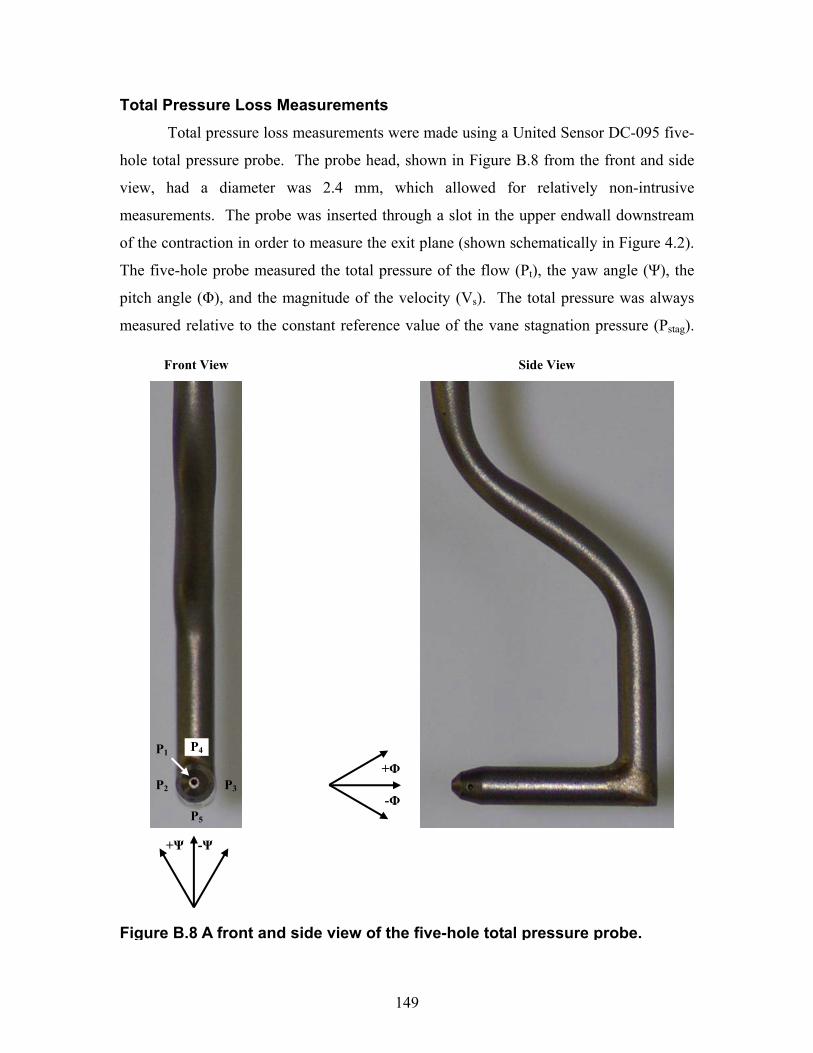
149

Total Pressure Loss Measurements Total pressure loss measurements were made using a United Sensor DC-095 five-

hole total pressure probe. The probe head, shown in Figure B.8 from the front and side

view, had a diameter was 2.4 mm, which allowed for relatively non-intrusive

measurements. The probe was inserted through a slot in the upper endwall downstream

of the contraction in order to measure the exit plane (shown schematically in Figure 4.2).

The five-hole probe measured the total pressure of the flow (Pt), the yaw angle (Ψ), the

pitch angle (Φ), and the magnitude of the velocity (Vs). The total pressure was always

measured relative to the constant reference value of the vane stagnation pressure (Pstag).

Figure B.8 A front and side view of the five-hole total pressure probe.

-Ψ +Ψ

-Φ

+Φ

Front View Side View

P1

P2 P3

P4

P5

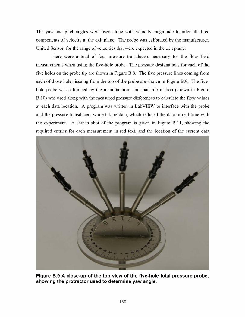
150

The yaw and pitch angles were used along with velocity magnitude to infer all three

components of velocity at the exit plane. The probe was calibrated by the manufacturer,

United Sensor, for the range of velocities that were expected in the exit plane.

There were a total of four pressure transducers necessary for the flow field

measurements when using the five-hole probe. The pressure designations for each of the

five holes on the probe tip are shown in Figure B.8. The five pressure lines coming from

each of those holes issuing from the top of the probe are shown in Figure B.9. The five-

hole probe was calibrated by the manufacturer, and that information (shown in Figure

B.10) was used along with the measured pressure differences to calculate the flow values

at each data location. A program was written in LabVIEW to interface with the probe

and the pressure transducers while taking data, which reduced the data in real-time with

the experiment. A screen shot of the program is given in Figure B.11, showing the

required entries for each measurement in red text, and the location of the current data

Figure B.9 A close-up of the top view of the five-hole total pressure probe, showing the protractor used to determine yaw angle.

151

point on the three calibration curve plots.

The first step in the data taking process was to determine the correct yaw (or flow

turning) angle. This was done manually by rotating the probe until the pressure

Figure B.10 Five-hole calibration data provided by United Sensor.

152

difference (P2 – P3) was equal to zero and reading the protractor attached to the top of the

probe (shown in Figure B.9). The yaw angle was manually entered into the LabVIEW

program, and used later to calculate secondary flow vectors.

After the correct yaw angle had been set, the pitch angle could then be calculated

from the ratio of measured pressure differences (P4 – P5)/(P1 – P23) using the calibration

data in Figure B.12. The pressure P23 was the average between P2 and P3, however, since

those two pressures are equalized in the first step to determine yaw angle, only P2 was

used for that pressure.

The pitch angle was then used to determine the velocity pressure coefficient using

Figure B.11 A screen-shot of the LabVIEW program written to take the five-hole probe measurements.

153

-45

-30

-15

0

15

30

45

-2.0 -1.5 -1.0 -0.5 0.0 0.5 1.0 1.5 2.0

Calibration Data

Φ

P4 - P

5

P1 - P

23

the calibration data given in Figure B.13, where the velocity pressure coefficient is given

by Equation B.7,

231

stvp PP

PPC−−

= (B.7)

The velocity pressure coefficient, Cvp and the measured pressure difference (P1 – P23)

were in turn used to calculate the dynamic pressure of the flow (Pt – Ps). The streamwise

velocity magnitude was then calculated from Equation B.8, a simplification of

Bernoulli’s Equation,

( )ρ−

= sts

PP2V (B.8)

where ρ was the freestream flow density, calculated by measuring the freestream

temperature and the atmospheric pressure and using the Ideal Gas Law.

Finally, the total pressure coefficient was determined using the pitch angle and the

calibration data shown in Figure B.14, where the total pressure coefficient was given by

Equation B.9,

Figure B.12 The calibration data used to determine the pitch angle from themeasured pressure differences.

154

0.90

0.95

1.00

1.05

1.10

-45 -30 -15 0 15 30 45

Calibration Data

Pt - P

s

P1 - P

23

Φ

-0.8

-0.6

-0.4

-0.2

0.0

0.2

-45 -30 -15 0 15 30 45

Calibration Data

P1 - P

t

Pt - P

s

Φ

Figure B.14 The calibration data used to determine the total pressurecoefficient from the measured pressure differences.

Figure B.13 The calibration data used to determine the velocity pressurecoefficient from the measured pressure differences.

155

st

t1tp PP

PPC−−

= (B.9)

The total pressure coefficient, Ctp, dynamic pressure of the flow, (Pt – Ps), and the

measured difference between P1 and the vane stagnation pressure (Pstag) were then used to

determine the pressure difference between the total pressure and the vane stagnation

pressure using Equation B.10,

( ) ( )[ ]sttpstag1stagt PPCPPPP −−−=− (B.10)

Nomenclature C coefficient of pressure

P pressure

Q radiation emitted from the surface measured by the infrared camera

S the surface distance around the vane, measured from the stagnation point

T temperature

V velocity

Greek

ε emissivity


ρ density

σ Stefan-Boltzmann constant (σ = 5.67x10-8 W·m2/K4)

Φ pitch angle

Ψ yaw angle

Subscripts

1 hole 1 on the five-hole probe





∞ freestream

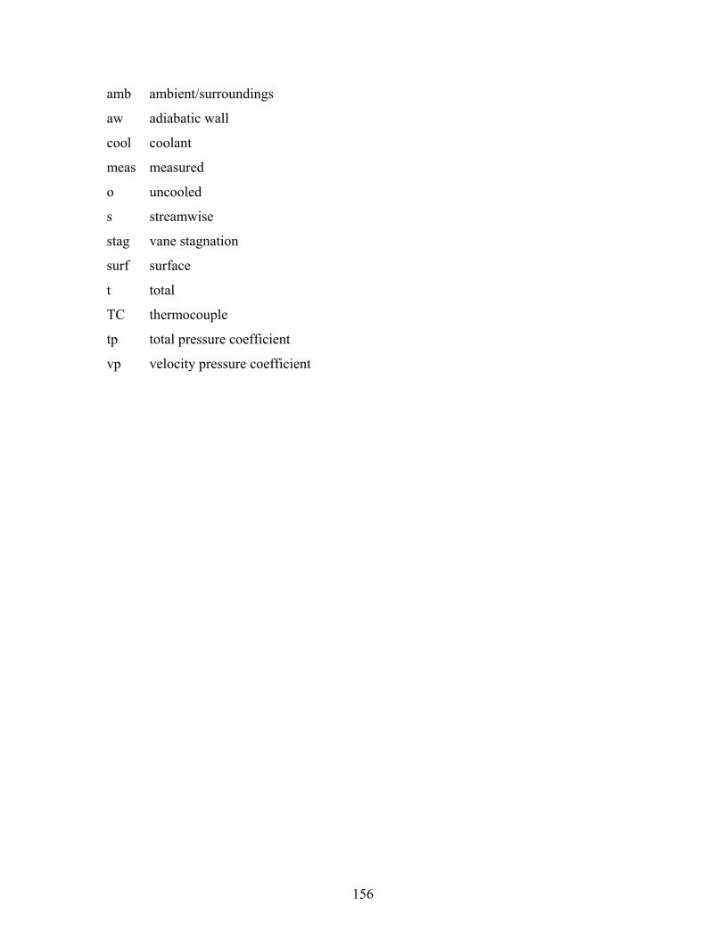
156

amb ambient/surroundings

aw adiabatic wall

cool coolant

meas measured

o uncooled

s streamwise

stag vane stagnation

surf surface

t total

TC thermocouple

tp total pressure coefficient

vp velocity pressure coefficient

157

Appendix C: Uncertainty Analysis of Experimental Results

Approach The uncertainty calculations for the experimental data presented in this

dissertation were performed using the method presented by Moffat [1]. This method took

into account the contribution of each variable used to calculate the reported value in

terms of its partial derivative. The parameter R was a reported value which was

calculated from measured values Xi and can be represented as shown in Equation C.1,

( )n21 X,,X,XRR L= (C.1)

The error in parameter R from any individual measured value Xi was given by Equation

C.2,

ii

i XXRR δ

∂∂

=δ (C.2)

Similarly, the total error in R as a function of all of the errors in the measured values used

to calculate R was just the root-sum-square of the individual errors associated with each

measured value (Equation C.3).

21

N

1i

2

ii

XXRR

δ

∂∂

=δ ∑=

(C.3)

The total uncertainty for the measurement of Xi was given by δXi, where δXi was the

root-sum-square of the bias uncertainty and the precision uncertainty in Xi. The bias

uncertainty for a measurement was defined as the capability of the measurement device

to accurately measure the true value. The precision uncertainty was defined as the

capability of the measurement device to repeat the same measurement of a property that

remained at the same value. The precision uncertainty was typically calculated by

measuring a single unchanging quantity a number of times, and taking the standard

deviation of those measurements.

Adiabatic Effectiveness – η

The measured film-cooling effectiveness for both the vane and the endwall

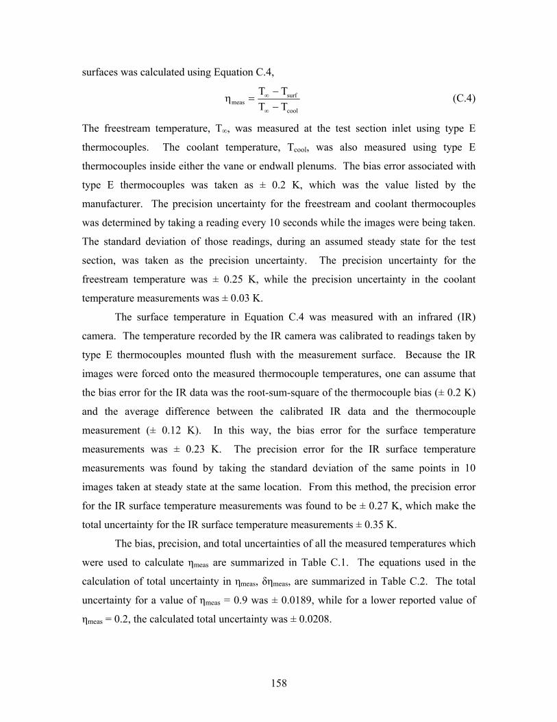
158

surfaces was calculated using Equation C.4,

cool

surfmeas TT

TT−−

=η∞

∞ (C.4)

The freestream temperature, T∞, was measured at the test section inlet using type E

thermocouples. The coolant temperature, Tcool, was also measured using type E

thermocouples inside either the vane or endwall plenums. The bias error associated with

type E thermocouples was taken as ± 0.2 K, which was the value listed by the

manufacturer. The precision uncertainty for the freestream and coolant thermocouples

was determined by taking a reading every 10 seconds while the images were being taken.

The standard deviation of those readings, during an assumed steady state for the test

section, was taken as the precision uncertainty. The precision uncertainty for the

freestream temperature was ± 0.25 K, while the precision uncertainty in the coolant

temperature measurements was ± 0.03 K.

The surface temperature in Equation C.4 was measured with an infrared (IR)

camera. The temperature recorded by the IR camera was calibrated to readings taken by

type E thermocouples mounted flush with the measurement surface. Because the IR

images were forced onto the measured thermocouple temperatures, one can assume that

the bias error for the IR data was the root-sum-square of the thermocouple bias (± 0.2 K)

and the average difference between the calibrated IR data and the thermocouple

measurement (± 0.12 K). In this way, the bias error for the surface temperature

measurements was ± 0.23 K. The precision error for the IR surface temperature

measurements was found by taking the standard deviation of the same points in 10

images taken at steady state at the same location. From this method, the precision error

for the IR surface temperature measurements was found to be ± 0.27 K, which make the

total uncertainty for the IR surface temperature measurements ± 0.35 K.

The bias, precision, and total uncertainties of all the measured temperatures which

were used to calculate ηmeas are summarized in Table C.1. The equations used in the

calculation of total uncertainty in ηmeas, δηmeas, are summarized in Table C.2. The total

uncertainty for a value of ηmeas = 0.9 was ± 0.0189, while for a lower reported value of

ηmeas = 0.2, the calculated total uncertainty was ± 0.0208.

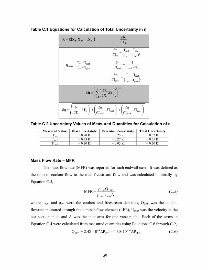
159

( ))n21 X,,X,XRR L= iX

R∂∂

cool

surfmeas TT

TT−−

=η∞

∞

( )2cool

coolsurf

TTTT

T −

−=

∂η∂

∞∞

∞−=

∂η∂

TT1

T coolsurf

( )2cool

surf

cool TTTT

T −

−=

∂η∂

∞

∞

21

N

1i

2

ii

XXRR

δ

∂∂

=δ ∑=

2

coolcool

2

surfsurf

2

TT

TT

TT

δ⋅

∂η∂

+

δ⋅

∂η∂

+

δ⋅

∂η∂

=δη ∞∞

Measured Value Bias Uncertainty Precision Uncertainty Total Uncertainty T¶ ± 0.20 K ± 0.25 K ± 0.32 K Tsurf ± 0.23 K ± 0.27 K ± 0.35 K Tcool ± 0.20 K ± 0.03 K ± 0.20 K

Mass Flow Rate – MFR The mass flow rate (MFR) was reported for each endwall case. It was defined as

the ratio of coolant flow to the total freestream flow and was calculated nominally by

Equation C.5,

AUQMFR

inlethot

LFEcool

ρρ

= (C.5)

where ρcool and ρhot were the coolant and freestream densities, QLFE was the coolant

flowrate measured through the laminar flow element (LFE), Uinlet was the velocity at the

test section inlet, and A was the inlet area for one vane pitch. Each of the terms in

Equation C.4 were calculated from measured quantities using Equations C.6 through C.9,

LFE10

LFE4

LFE P1030.4P1048.2Q ∆⋅−∆⋅= −− (C.6)

Table C.1 Equations for Calculation of Total Uncertainty in η

Table C.2 Uncertainty Values of Measured Quantities for Calculation of η

160

cool

atmcool RT

P=ρ (C.7)

hot

atmhot RT

P=ρ (C.8)

hot

Pitotinlet

P2Uρ∆

= (C.9)

The atmospheric pressure, Patm, was measured with a digital Setra pressure

transducer with a range from 800 mbar to 1100 mbar. The bias uncertainty in the reading

was ± 0.0206% of the full scale (also ± 0.0681 mbar or ± 6.81 Pa). The precision

uncertainty was determined by measuring the same pressure 20 times, once every 10

seconds and determined from the standard deviation of that data to be ± 1.88 Pa. That

makes a total uncertainty in the measurement of atmospheric pressure of ± 7.06 Pa.

The freestream temperature, Thot, was measured with type E thermocouples at the

inlet. Again, the manufacturer specified value for bias uncertainty in type E

thermocouples was ± 0.2 K. The precision uncertainty was determined from the raw data

file which records temperatures continuously during testing and was ± 0.27 K. The total

uncertainty was therefore ± 0.34 K.

The coolant temperature, Tcool, was measured with two type E thermocouples

located inside the endwall plenum and positioned just below the entrance to the holes.

The precision uncertainty was determined from the raw data file which records

temperatures continuously during testing and was ± 0.08 K. The total uncertainty was

therefore ± 0.22 K.

The pressure drop through the LFE was measured using a 5.0" Setra pressure

transducer, which had a bias uncertainty of ± 0.206% of the full scale (or ± 0.64 Pa). The

precision error was not measured; however, it could be inferred from the Pitot probe

measurements made with the 0.25" transducer as ± 0.78 Pa, which makes the total

uncertainty ± 1.01 Pa.

The inlet velocity was measured indirectly by measuring the inlet dynamic

pressure at the inlet with a Pitot probe. A 0.25" Setra pressure transducer was used to

make the measurements. The pressure transducer has a bias error of ± 0.206% of the full

scale (or ± 0.13 Pa). The inlet profile was used to calculate a precision error of ± 0.18 Pa.

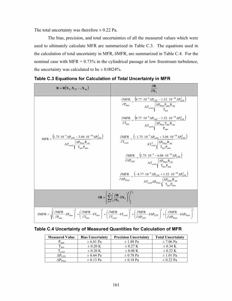
161

The total uncertainty was therefore ± 0.22 Pa.

The bias, precision, and total uncertainties of all the measured values which were

used to ultimately calculate MFR are summarized in Table C.3. The equations used in

the calculation of total uncertainty in MFR, δMFR, are summarized in Table C.4. For the

nominal case with MFR = 0.73% in the cylindrical passage at low freestream turbulence,

the uncertainty was calculated to be ± 0.0024%.


R∂∂

( )

atmhot

airPitotcool

2LFE

10LFE

5

PTRPAT

P1004.3P1075.1MFR∆

∆⋅−∆⋅=

−−

( )

hot

airatmPitotcool

2LFE

10LFE

6

atm

TRPPAT

P1052.1P1077.8P

MFR∆

∆⋅−∆⋅=

∂∂ −−

( )

atm

airhotPitotcool

2LFE

10LFE

6

hot

PRTPAT

P1052.1P1077.8T

MFR∆

∆⋅−∆⋅=

∂∂ −−

( )

atmhot

airPitot2cool

2LFE

10LFE

5

cool

PTRPAT

P1004.3P1075.1TMFR

∆∆⋅+∆⋅−

=∂∂ −−

( )

atmhot

airPitotcool

LFE105

LFE

PTRPAT

P1008.61075.1P

MFR∆

∆⋅−⋅=

∆∂∂ −−

( )

atmhot

airPitotPitotcool

2LFE

10LFE

6

Pitot

PTRPPAT

P1052.1P1077.8P

MFR∆

∆

∆⋅+∆⋅−=

∆∂∂ −−

21

N

1i

2

ii

XXRR

δ

∂∂

=δ ∑=

2

PitotPitot

2

LFELFE

2

coolcool

2

hothot

2

atmatm

PP

MFRPP

MFRTTMFRT

TMFRP

PMFRMFR

∆δ⋅

∆∂∂

+

∆δ⋅

∆∂∂

+

δ⋅

∂∂

+

δ⋅

∂∂

+

δ⋅

∂∂

=δ

Measured Value Bias Uncertainty Precision Uncertainty Total Uncertainty Patm ± 6.81 Pa ± 1.88 Pa ± 7.06 Pa Thot ± 0.20 K ± 0.27 K ± 0.34 K Tcool ± 0.20 K ± 0.08 K ± 0.22 K ∆PLFE ± 0.64 Pa ± 0.78 Pa ± 1.01 Pa ∆PPitot ± 0.13 Pa ± 0.18 Pa ± 0.22 Pa

Table C.3 Equations for Calculation of Total Uncertainty in MFR

Table C.4 Uncertainty of Measured Quantities for Calculation of MFR

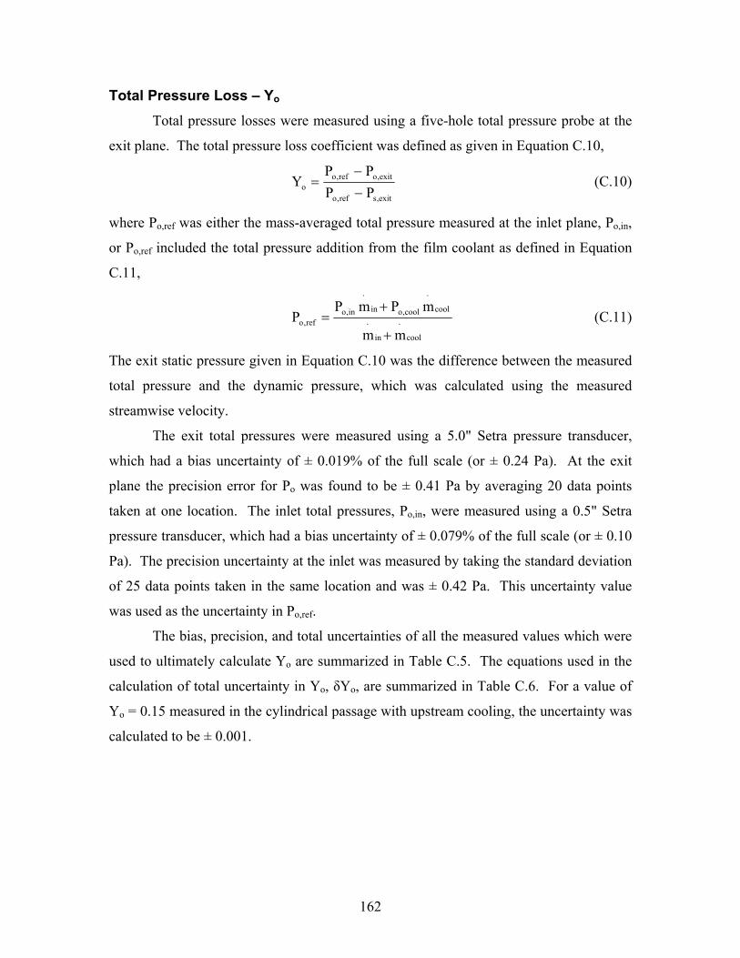
162

Total Pressure Loss – Yo Total pressure losses were measured using a five-hole total pressure probe at the

exit plane. The total pressure loss coefficient was defined as given in Equation C.10,

exit,sref,o

exit,oref,oo PP

PPY

−−

= (C.10)

where Po,ref was either the mass-averaged total pressure measured at the inlet plane, Po,in,

or Po,ref included the total pressure addition from the film coolant as defined in Equation

C.11,

coolin

coolcool,oinin,oref,o

mm

mPmPP ⋅⋅

⋅⋅

+

+= (C.11)

The exit static pressure given in Equation C.10 was the difference between the measured

total pressure and the dynamic pressure, which was calculated using the measured

streamwise velocity.

The exit total pressures were measured using a 5.0" Setra pressure transducer,

which had a bias uncertainty of ± 0.019% of the full scale (or ± 0.24 Pa). At the exit

plane the precision error for Po was found to be ± 0.41 Pa by averaging 20 data points

taken at one location. The inlet total pressures, Po,in, were measured using a 0.5" Setra

pressure transducer, which had a bias uncertainty of ± 0.079% of the full scale (or ± 0.10

Pa). The precision uncertainty at the inlet was measured by taking the standard deviation

of 25 data points taken in the same location and was ± 0.42 Pa. This uncertainty value

was used as the uncertainty in Po,ref.

The bias, precision, and total uncertainties of all the measured values which were

used to ultimately calculate Yo are summarized in Table C.5. The equations used in the

calculation of total uncertainty in Yo, δYo, are summarized in Table C.6. For a value of

Yo = 0.15 measured in the cylindrical passage with upstream cooling, the uncertainty was

calculated to be ± 0.001.

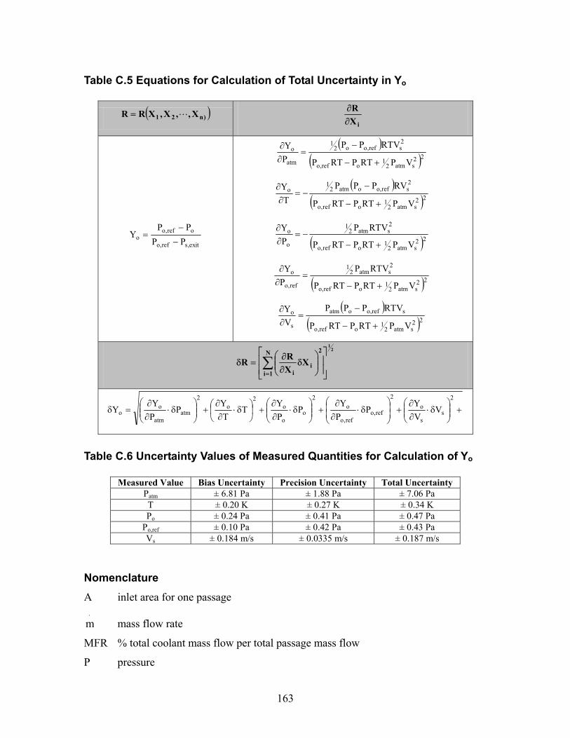
163


R∂∂

exit,sref,o

oref,oo PP

PPY

−

−=

( )( )22

satm21

oref,o

2sref,oo2

1

atm

o

VPRTPRTP

RTVPPPY

+−

−=

∂∂

( )( )22

satm21

oref,o

2sref,ooatm2

1o

VPRTPRTP

RVPPPT

Y

+−

−−=

∂∂

( )22satm2

1oref,o

2satm2

1

o

o

VPRTPRTP

RTVPPY

+−−=

∂∂

( )22satm2

1oref,o

2satm2

1

ref,o

o

VPRTPRTP

RTVPPY

+−=

∂∂

( )( )22

satm21

oref,o

sref,ooatm

s

o

VPRTPRTP

RTVPPPVY

+−

−=

∂∂

21

N

1i

2

ii

XXRR

δ

∂∂

=δ ∑=

+

δ⋅

∂∂

+

δ⋅

∂∂

+

δ⋅

∂∂

+

δ⋅∂∂

+

δ⋅

∂∂

=δ2

ss

o2

ref,oref,o

o2

oo

o2

o2

atmatm

oo V

VY

PPY

PPY

TT

YP

PY

Y

Measured Value Bias Uncertainty Precision Uncertainty Total Uncertainty

Patm ± 6.81 Pa ± 1.88 Pa ± 7.06 Pa T ± 0.20 K ± 0.27 K ± 0.34 K Po ± 0.24 Pa ± 0.41 Pa ± 0.47 Pa

Po,ref ± 0.10 Pa ± 0.42 Pa ± 0.43 Pa Vs ± 0.184 m/s ± 0.0335 m/s ± 0.187 m/s

Nomenclature A inlet area for one passage ⋅

m mass flow rate


P pressure

Table C.5 Equations for Calculation of Total Uncertainty in Yo

Table C.6 Uncertainty Values of Measured Quantities for Calculation of Yo

164

Q volumetric flowrate

R a reported parameter calculated from measured values/ideal gas constant

T temperature

U velocity

Vs streamwise velocity

X any measured value

Yo total pressure loss coefficient, Yo = (Po,ref – Po,exit)/ (Po,ref – Ps,exit)

Greek

δ experimental error

∆ change in

η adiabatic film-cooling effectiveness, ηmeas = (T∞ – Tsurf)/(T∞ – Tcool)

ρ density

Subscripts

1 the first index number

2 the second index number

∞ freestream

atm atmospheric

cool coolant

exit exit plane

hot hot gas

i an index number

in inlet condition

inlet inlet condition

LFE laminar flow element

meas measured value

n the nth index number

N the total number of measured values that are included in calculating R

o total

Pitot measured with a Pitot probe

165

ref reference value

s static

surf surface

References [1] Moffat, R. J., 1988, “Describing the Uncertainties in Experimental Results,”

Experimental Thermal and Fluid Science, vol. 1, pp. 3-17.

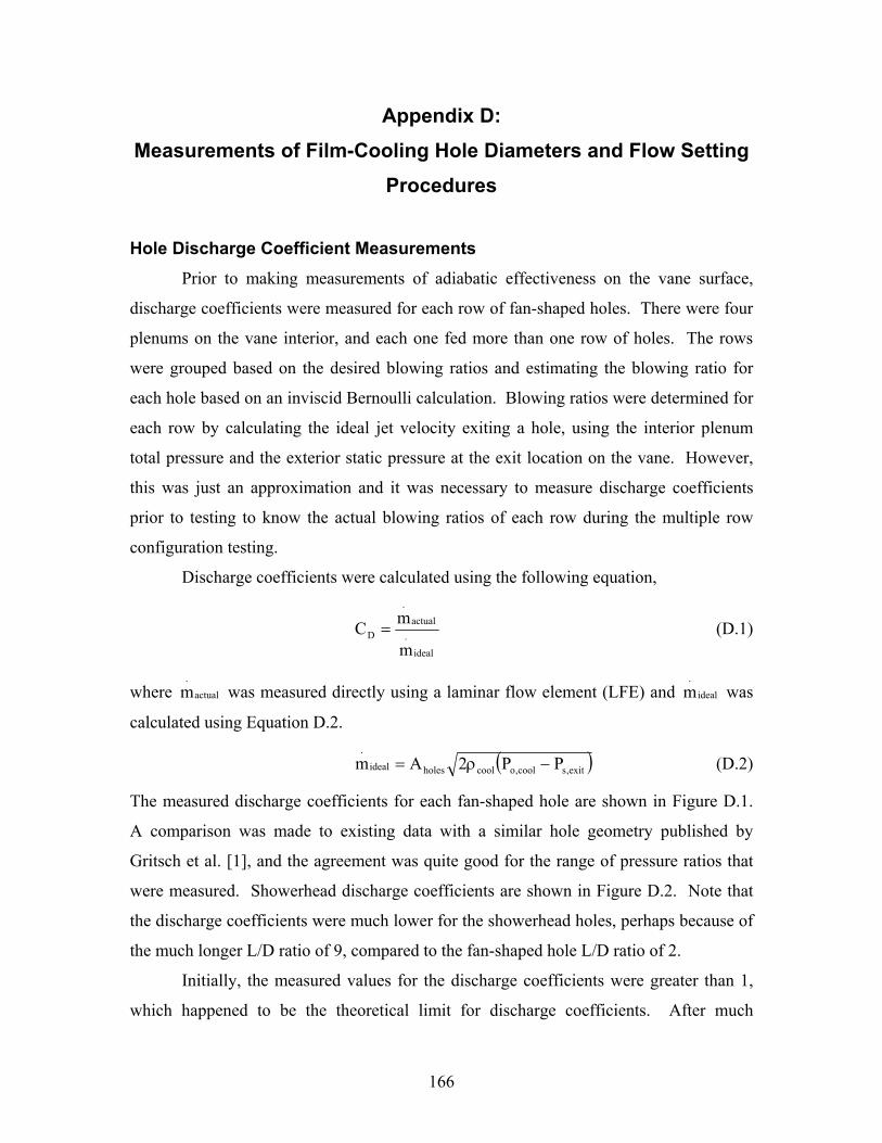
166

Appendix D: Measurements of Film-Cooling Hole Diameters and Flow Setting

Procedures

Hole Discharge Coefficient Measurements Prior to making measurements of adiabatic effectiveness on the vane surface,

discharge coefficients were measured for each row of fan-shaped holes. There were four

plenums on the vane interior, and each one fed more than one row of holes. The rows

were grouped based on the desired blowing ratios and estimating the blowing ratio for

each hole based on an inviscid Bernoulli calculation. Blowing ratios were determined for

each row by calculating the ideal jet velocity exiting a hole, using the interior plenum

total pressure and the exterior static pressure at the exit location on the vane. However,

this was just an approximation and it was necessary to measure discharge coefficients

prior to testing to know the actual blowing ratios of each row during the multiple row

configuration testing.

Discharge coefficients were calculated using the following equation,

ideal.

actual.

D

m

mC = (D.1)

where actual.

m was measured directly using a laminar flow element (LFE) and ideal.

m was

calculated using Equation D.2.

( )exit,scool,ocoolholesideal.

PP2Am −ρ= (D.2)

The measured discharge coefficients for each fan-shaped hole are shown in Figure D.1.

A comparison was made to existing data with a similar hole geometry published by

Gritsch et al. [1], and the agreement was quite good for the range of pressure ratios that

were measured. Showerhead discharge coefficients are shown in Figure D.2. Note that

the discharge coefficients were much lower for the showerhead holes, perhaps because of

the much longer L/D ratio of 9, compared to the fan-shaped hole L/D ratio of 2.

Initially, the measured values for the discharge coefficients were greater than 1,

which happened to be the theoretical limit for discharge coefficients. After much

167

0.0

0.2

0.4

0.6

0.8

1.0

1.00 1.02 1.04 1.06 1.08 1.10

Row PARow PBRow PCRow PDRow SARow SBRow SCRow SDFan Shaped, Gritsch et al. [1]Laidback Fan Shaped, Gritsch et al. [1]

po,cool

/ps,exit

CD

0.0

0.2

0.4

0.6

0.8

1.0

1.000 1.005 1.010 1.015

Row HARow HBRow HCRow HDRow HE

po,cool

/ps,exit

CD

investigation for leakage through the piping and plenum interior, the problem was

determined to be inaccurate knowledge of the cooling hole diameter. The term Aholes in

Equation D.2 was defined as the metering area, so the specified value given to the

Figure D.2 Showerhead hole discharge coefficients.

Figure D.1 Fan-shaped hole discharge coefficients.

168

manufacturer was used for the calculations. Upon closer examination, it was determined

that some of the holes were slightly larger, however, at the experimental scale of the vane

it had a large effect on the outcome of CD. In addition, some of the holes did not have

circular cross-sections at the metering area (Figure D.3). The irregularities were most

likely a result of either the manufacturing or the instrumentation process.

Hole Diameter Measurements In order to get correct values for the average discharge coefficient of each row,

every hole was measured with extremely accurate pin gages. The circular pins increased

in diameter in increments of approximately 0.03 mm. The non-circular irregularities

were also accounted for, both the distorted corners and the ovular hole shapes. The

distorted corners were approximated by assuming any irregular shape in a quadrant of the

circular cross-section to have a square corner. The area of any ovular hole was calculated

by measuring the major (D1) and minor (D2) axis, and using Equation D.3,

21oval DD4

A π= (D.3)

Both irregularities are illustrated schematically in Figure D.4.

The final results for the hole diameter measurement process are listed in Table

D.1. In summary, the specified fan-shaped hole diameter in the circular entrance length

region was given as 2.61 mm. The average measured diameter in that same region for the

Figure D.3 Example of two non-circular holes at the metering area. The upper hole has an ovular shape, while the lower left-hand quadrant of the lower hole was approximated as a square.

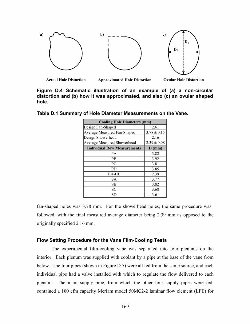
169

Cooling Hole Diameters (mm) Design Fan-Shaped 2.61 Average Measured Fan-Shaped 3.78 ± 0.15Design Showerhead 2.16 Average Measured Showerhead 2.39 ± 0.08

Individual Row Measurements D (mm) PA 3.82 PB 3.92 PC 3.81 PD 3.85

HA-HE 2.39 SA 3.77 SB 3.82 SC 3.68 SD 3.61

fan-shaped holes was 3.78 mm. For the showerhead holes, the same procedure was

followed, with the final measured average diameter being 2.39 mm as opposed to the

originally specified 2.16 mm.

Flow Setting Procedure for the Vane Film-Cooling Tests The experimental film-cooling vane was separated into four plenums on the

interior. Each plenum was supplied with coolant by a pipe at the base of the vane from

below. The four pipes (shown in Figure D.5) were all fed from the same source, and each

individual pipe had a valve installed with which to regulate the flow delivered to each

plenum. The main supply pipe, from which the other four supply pipes were fed,

contained a 100 cfm capacity Meriam model 50MC2-2 laminar flow element (LFE) for

Table D.1 Summary of Hole Diameter Measurements on the Vane.

Actual Hole Distortion Approximated Hole Distortion

D1

D2

Ovular Hole Distortion

a) b) c)

Figure D.4 Schematic illustration of an example of (a) a non-circular distortion and (b) how it was approximated, and also (c) an ovular shapedhole.

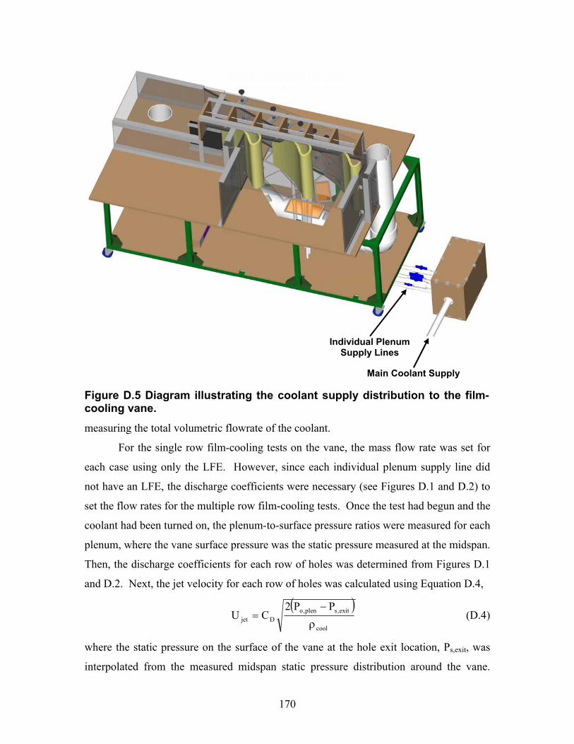
170

measuring the total volumetric flowrate of the coolant.

For the single row film-cooling tests on the vane, the mass flow rate was set for

each case using only the LFE. However, since each individual plenum supply line did

not have an LFE, the discharge coefficients were necessary (see Figures D.1 and D.2) to

set the flow rates for the multiple row film-cooling tests. Once the test had begun and the

coolant had been turned on, the plenum-to-surface pressure ratios were measured for each

plenum, where the vane surface pressure was the static pressure measured at the midspan.

Then, the discharge coefficients for each row of holes was determined from Figures D.1

and D.2. Next, the jet velocity for each row of holes was calculated using Equation D.4,

( )cool

exit,splen,oDjet

PP2CU

ρ

−= (D.4)

where the static pressure on the surface of the vane at the hole exit location, Ps,exit, was

interpolated from the measured midspan static pressure distribution around the vane.

Figure D.5 Diagram illustrating the coolant supply distribution to the film-cooling vane.

Main Coolant Supply

Individual Plenum Supply Lines

171

Pressure taps were located within each plenum with which to measure the plenum total

pressure, Po,plen. The blowing ratios at each hole were then calculated using Equation

D.5,

local

jetcool

UU

M∞ρ

ρ= (D.4)

where the local velocity near the surface of the vane at the hole exit, Ulocal, was calculated

using the measured static pressure distribution around the vane.

The measured blowing ratios at each hole location were then compared to the

desired values. The valves for each coolant supply pipe were then adjusted to minimize

the difference between the calculated blowing ratios and the desired blowing ratios.

Once the flows had been set, the total coolant mass flow to the vane measured with the

LFE was compared with the calculated total mass flow rate using the measured pressure

ratios and discharge coefficients. The difference between the actual measured value and

the predicted calculated value was always less than 2% for all multiple row vane film-

cooling experiments.

Flow Setting Procedure for the Endwall Film-Cooling Tests

The endwall film-cooling tests required a plenum to be built underneath the lower

flat film-cooled endwall. The plenum is shown in Figure D.6, along with the single

coolant supply pipe for the plenum. Each coolant passage could be totally blocked from

inside the plenum, with specially designed Lexan plates which covered the hole

entrances. The coolant supply pipe contained the same Meriam model 50MC2-2 LFE, so

the mass flow rate for each test could be measured directly, as long as the passage that

was not being tested was blocked from within the plenum.

Similarly, for the tests without upstream coolant injection, the upstream film-

cooling holes were selectively blocked from within the plenum on the passage to be

tested. In addition, the holes for the untested passage were also blocked. The pressure

ratio taken from within the plenum relative to static pressure taps located 0.6 C upstream

of the vane stagnation was matched to the cases with upstream injection. In this way, the

unblocked cooling holes within the passage had the same coolant flow regardless of the

status of the upstream cooling holes.

172

Nomenclature A inlet area for one passage

C true vane chord

CD discharge coefficient, CD = actualm⋅

/ idealm⋅

D diameter at the hole inlet

L metering length of the hole ⋅

m mass flow rate

P pressure

U velocity

Figure D.6 Illustration of the endwall coolant plenum showing the single coolant supply line (the other inlet pipes that are shown were blocked andnot used).

Coolant Inlet

173

Greek

ρ density

Subscripts

1 the major axis of an oval

2 the minor axis of an oval

actual the actual flowrate that occurs through the hole because of losses

cool coolant

exit exit of the hole

holes all film-cooling holes in an individual row

ideal the ideal flow rate through the hole as predicted by the Bernoulli Equation

jet film-cooling jet at the metering area

o total

oval the cross-sectional area of an oval

plen plenum

s static

References [1] Gritsch, M., Schulz, A., and Wittig, S., 1997, “Discharge Coefficient

Measurements of Film-Cooling Holes with Expanded Exits,” 97-GT-165.

174

Vita

William Frederick Colban IV Will was born on November 6, 1980 in Beaufort, SC, son of Michelle Pauline

Colban-Hill and William Frederick Colban III. On May 25, 1992, Will’s brother Ellis

‘EJ’ Hill II was born. Will went to high school in Richmond, VA at the Governor’s

School, graduating in 1997. Wanting to study mechanical engineering, Will decided to

attend renowned Virginia Tech.

Four years later, in May 2001, Will graduated with a BSME from Virginia Tech.

Because of his insatiable thirst to understand the physical world around him, Will

continued on as a graduate student, receiving his MSME in the January 2002. During

that time, in the fall of 2001, he met the girl that he would ultimately ask to marry him,

the beautiful Lauren Elizabeth Ross.

The following spring in 2002, Will went to Baden, Switzerland to work as an

intern for ALSTOM Power. Will had always wanted to go live and travel in Europe, and

he got the opportunity to see many different countries and meet people from all over the

world. During that time, Will decided he would return to Virginia Tech to work on a

PhD in mechanical engineering under Dr. Karen A. Thole. Will’s research centered on

the examination of fan-shaped film-cooling holes in a gas turbine vane, and he learned a

great deal.

On July 3, 2005 Will asked Lauren to marry him at the Middleton Inn in

Charleston, SC. The following December, Will received his PhD in mechanical

engineering from the great Virginia Polytechnic Institute and State University.

Documents

A Detailed Study of Fan-Shaped Film-Cooling for a … cool the critical turbine surfaces, while at the same time extracting more benefit from the coolant flow that is used. Fan-shaped