A Design-of-Experiments Plug-In for Estimating Uncertainties in Finite Element Simulations · 2009-10-26 · A Design-of-Experiments Plug-In for Estimating Uncertainties in Finite

2009 SIMULIA Customer Conference 1

A Design-of-Experiments Plug-In for EstimatingUncertainties in Finite Element Simulations (*)

Jeffrey T. Fong1, Roland deWit1, Pedro V. Marcal2, James J. Filliben1, andN. Alan Heckert1

1National Institute of Standards and Technology, Gaithersburg, MD 20899 U.S.A.2MPave Corp, Julian, CA 92036 U.S.A.

Abstract: The objective of this paper is to introduce an economical and user-friendly techniquefor estimating a specific type of finite element simulation uncertainties, or, "error bars," for aclass of mathematical models, of which no closed-form or approximate solution is known to exist.Using Python, Abaqus-Python, and a public-domain statistical data analysis software packagenamed Dataplot, we present a design-of-experiments-based Python-Dataplot-Uncertainty Plug-In(PD-UP) to estimate the finite element simulation uncertainties in a mathematical model due tovariability in modeling parameters such as material property constants, geometric parameters,loading rates, etc. Examples of finite element simulations of the free vibrations of a single-crystalsilicon cantilever beam in an atomic force microscope with an estimation of the uncertainties ofthe first bending mode resonance frequency of the beam, are included.

Keywords: Abaqus; ANSYS; atomic force microscope, cantilever beam; computational sciences;Dataplot; design of experiments; finite element method; mathematical modeling; mechanics;nanotechnology; plug-in; Python; sensitivity analysis; simulation; single crystal silicon; statisticaldata analysis; uncertainty analysis; uncertainty quantification; verification; vibration.

(*) Contribution of National Institute of Standards and Technology. Not subject to copyright.

1. Introduction

It is well-known that simulation results of the finite element method (FEM) contain errors due to avariety of sources (see, e.g., Hughes 1987, Haldar 1997, Zienkiewicz 2000, Chu 2002, Yang 2002,Lord 2003, Fong 2005, Fong 2006a, Fong 2006b, Fong 2008a). By and large, such errors are ofmajor concern to experimentalists or modelers, when the governing equations and their associatedmaterial property constants, boundary conditions, geometric parameters, and loading rates, etc.,are known to contain significant uncertainties as defined for physical measurements in ISO 1993and Taylor 1994, and for black-box computer models by a recent paper of Kennedy 2001. In thispaper, we address FEM simulation errors by going beyond Kennedy 2001 in the sense that we nolonger treat an FEM model as a black-box. Using a design-of-experiments approach and a 10-stepstatistical analysis algorithm (Filliben 2002), we develop a plug-in for an FEM model with anuncertainty estimation and a robustness ranking of not only the parametric variables but also theFEM code platforms (e.g., Abaqus vs. ANSYS) and FEM mesh sizes (coarse vs. fine).

2 2009 SIMULIA Customer Conference

2. A Calibrated FEM Model

In the opening section of a 2001 paper by Kennedy and O'Hagan (Kennedy 2001), the authorsmade the following observation on "computer models and calibration":

" . . . to use a model to make predictions in a specific context it may be necessary first tocalibrate the model by using some observed data." [Italics by authors of this paper.]

Kennedy and O'Hagan went on to present a "Bayesian approach to calibrating a computer code byusing observations from the real process, and subsequent prediction and uncertainty analysis of theprocess whcih corrects for model inadequacy." They treated the computer code as a "black box,"and made no use of information about the mathematical model implemented by the code.

Our interest in developing a calibrated FEM model requires us to open up that "black box" andhave a closer look at the output of that model as it varies according to three metrics, namely, thefinite element mesh size, m , the mesh type, mt , (e.g., hexahedron vs. tetrahedron), and the FEMcode implementation type, c t , (e.g., Abaqus vs. ANSYS). To facilitate our presentation, we adoptthe notation of Kennedy and O'Hagan (see Sections 4.1 and 4.2 of Kennedy 2001) with a minorchange in indexing the components of various vectors to avoid confusion with our notation inprior publications using the method of design of experiments (Fong 2006b, Fong 2008a).

Let x = (x1, . . ., xk)T be a k-dimensional process input vector, and t = (t1, . . ., tq2)T, a q2-

dimensional calibration input vector, such that n runs of a computer code produces an outputvector y = (y1, . . ., yn)

T given by the following relation:

y = (x, t). (1)

Let (x) denote the true value of a real process when the variable process inputs take values x ,and let there be no observations denoted by the no-dimensional vector, z = (z1, . . ., zno)

T , whereeach zp , p = 1, . . ., no, is an observation of (x) for known variable inputs x , but subject toerror. The full set of data that is available for the analysis is dT = (yT, zT), and according toKennedy 2001, the relationship between the observations zp , the true process (x) , and thecomputer model output (x, t), is given by the following equation:

zp = (x) + ep = (x,) + (x) + ep , (2)

where ep is the observation error for the pth observation, is an unknown regressionparameter, and (x) is a model inadequacy function that is independent of the code output (x,), and is the unknown calibration inputs corresponding to the particular real process forwhich we wish to calibrate the model. Note that when we make the n runs of the computermodel, we replace by t , the known values of the calibration inputs, and as pointed out inKennedy 2001, the important conceptual difference between and t requires us to emphasize itin equation (2), which can be viewed as defining a non-linear regression model. The computercode itself defines the regression function through the term (x, ), with parameters and .The other two terms can be viewed as together representing (non-independent) residuals.


3. A Calibrated FEM Model for a "Simple" Real Process

To illustrate the various quantities in equation (2) in a simple example, let us assume a "simple"real process where a mathematical model exists with a known solution such that both (x) and epin equation (2) vanish. In addition, we consider a sufficiently small local region where a linearregression model is valid ( = 1), then equation (2) for an FEM model with a two-dimensionalinput vector, (X1, X2)

T, may be written in the following form:

z = (x, t) + (x) + e = A0 + A1 * X1 , + A2 * X2 + t ( m, mt , ct ;, e ), (3)

where A0 , A1, and A2 are the regression coefficients of a linear model, and t , a calibrationinput function that could depend on the FEM mesh size, m , mesh type, mt , the code implementa-tion type, ct , as well as and e . In general, the dimension of the input vector in Equation (3)may be more than two, but for the purpose of illustrating equation (2), we shall present examplesonly for a two-dimensional input vector.

4. Statistical Theory of Design of Experiments (abbrev. DOE)

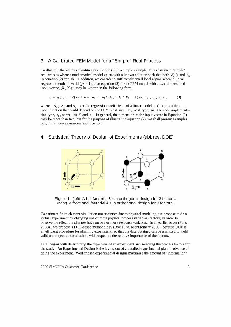
Figure 1. (left) A full-factorial 8-run orthogonal design for 3 factors.(right) A fractional factorial 4-run orthogonal design for 3 factors.

To estimate finite element simulation uncertainties due to physical modeling, we propose to do avirtual experiment by changing one or more physical process variables (factors) in order toobserve the effect the changes have on one or more response variables. In an earlier paper (Fong2008a), we propose a DOE-based methodology (Box 1978, Montgomery 2000), because DOE isan efficient procedure for planning experiments so that the data obtained can be analyzed to yieldvalid and objective conclusions with respect to the relative importance of the factors.

DOE begins with determining the objectives of an experiment and selecting the process factors forthe study. An Experimental Design is the laying out of a detailed experimental plan in advance ofdoing the experiment. Well chosen experimental designs maximize the amount of "information"


that can be obtained for a given amount of experimental effort. The statistical theory underlyingDOE begins with the concept of process models. A process model of the 'black box' type isformulated with several discrete or continuous input factors that can be controlled, and one ormore measured output responses. The output responses are assumed continuous. Real or virtualexperimental data are used to derive an empirical (approximate) model linking the outputs andinputs. These empirical models generally contain first-order (linear) and second-order (quadraticand interactions) terms. For a complete exposition of this topic, readers are referred to the articles(Box 1978, Montgomery 2000, Croarkin 2003, Fong 2008a) cited in Section 12 (References)

The most popular and cost-effective experimental designs for sensitivity analysis are two-leveldesigns. To illustrate the concept, we show in Fig. 1 (left) a graphical representation of a two-level, full factorial design for three factors, namely, the 23 design, and Fig. 4 (right) the same of atwo-level, fractional factorial design, or, the 23-1 design. The arrows show the direction ofincrease of the factors in order to represent the user-defined variability of each factor. Thenumbers "1" through "8" at the corners of the design box refer to the "Standing Order" of runs(also known in the literature as the "Yates Order").

5. A Calibrated FEM Model of Free Vibrations of a Cantilever Beam

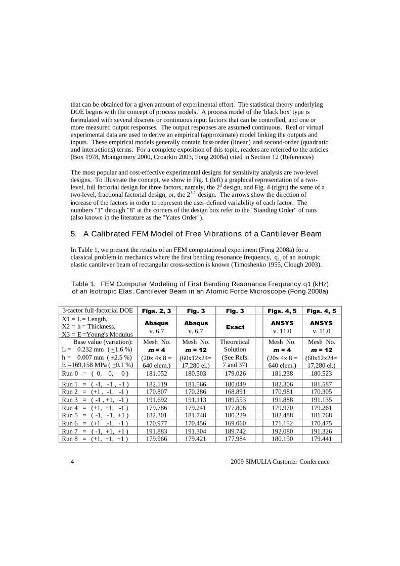
In Table 1, we present the results of an FEM computational experiment (Fong 2008a) for aclassical problem in mechanics where the first bending resonance frequency, q1, of an isotropicelastic cantilever beam of rectangular cross-section is known (Timoshenko 1955, Clough 2003).

Table 1. FEM Computer Modeling of First Bending Resonance Frequency q1 (kHz)of an Isotropic Elas. Cantilever Beam in an Atomic Force Microscope (Fong 2008a)

3-factor full-factorial DOE Figs. 2, 3 Fig. 3 Fig. 3 Figs. 4, 5 Figs. 4, 5X1 = L = Length,X2 = h = Thickness,X3 = E =Young's Modulus

Abaqusv. 6.7

Abaqusv. 6.7

ExactANSYSv. 11.0

ANSYSv. 11.0

Base value (variation):L = 0.232 mm ( +1.6 %)h = 0.007 mm ( +2.5 %)E =169,158 MPa ( +0.1 %)

Mesh No.m = 4

(20x 4x 8 =640 elem.)

Mesh No.m = 12

(60x12x24=17,280 el.)

TheoreticalSolution

(See Refs.7 and 37)

Mesh No.m = 4

(20x 4x 8 =640 elem.)

Mesh No.m = 12

(60x12x24=17,280 el.)

Run 0 = ( 0, 0, 0 ) 181.052 180.503 179.026 181.238 180.523

Run 1 = ( -1, -1 , -1 ) 182.119 181.566 180.049 182.306 181.587Run 2 = (+1 , -1, -1 ) 170.807 170.286 168.891 170.981 170.305Run 3 = ( -1 , +1, -1 ) 191.692 191.113 189.553 191.888 191.135Run 4 = (+1, +1, -1 ) 179.786 179.241 177.806 179.970 179.261Run 5 = ( -1, -1, +1 ) 182.301 181.748 180.229 182.488 181.768Run 6 = (+1 ,-1, +1 ) 170.977 170.456 169.060 171.152 170.475Run 7 = ( -1, +1, +1 ) 191.883 191.304 189.742 192.080 191.326Run 8 = (+1, +1, +1 ) 179.966 179.421 177.984 180.150 179.441


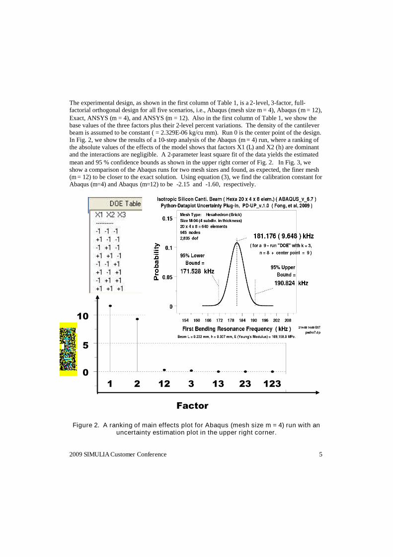
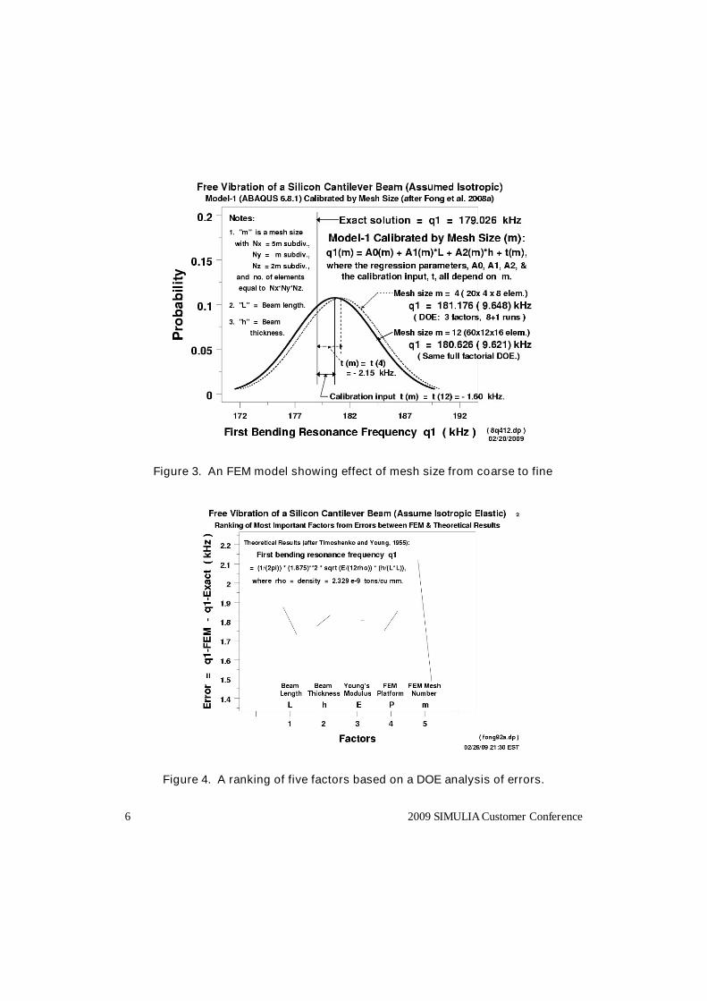
The experimental design, as shown in the first column of Table 1, is a 2-level, 3-factor, full-factorial orthogonal design for all five scenarios, i.e., Abaqus (mesh size m = 4), Abaqus (m = 12),Exact, ANSYS (m = 4), and ANSYS (m = 12). Also in the first column of Table 1, we show thebase values of the three factors plus their 2-level percent variations. The density of the cantileverbeam is assumed to be constant ( = 2.329E-06 kg/cu mm). Run 0 is the center point of the design.In Fig. 2, we show the results of a 10-step analysis of the Abaqus (m = 4) run, where a ranking ofthe absolute values of the effects of the model shows that factors X1 (L) and X2 (h) are dominantand the interactions are negligible. A 2-parameter least square fit of the data yields the estimatedmean and 95 % confidence bounds as shown in the upper right corner of Fig. 2. In Fig. 3, weshow a comparison of the Abaqus runs for two mesh sizes and found, as expected, the finer mesh(m = 12) to be closer to the exact solution. Using equation (3), we find the calibration constant forAbaqus (m=4) and Abaqus (m=12) to be -2.15 and -1.60, respectively.

Figure 2. A ranking of main effects plot for Abaqus (mesh size m = 4) run with anuncertainty estimation plot in the upper right corner.

10

5

01 2 12 3 13 23 123

Factor


Figure 3. An FEM model showing effect of mesh size from coarse to fine

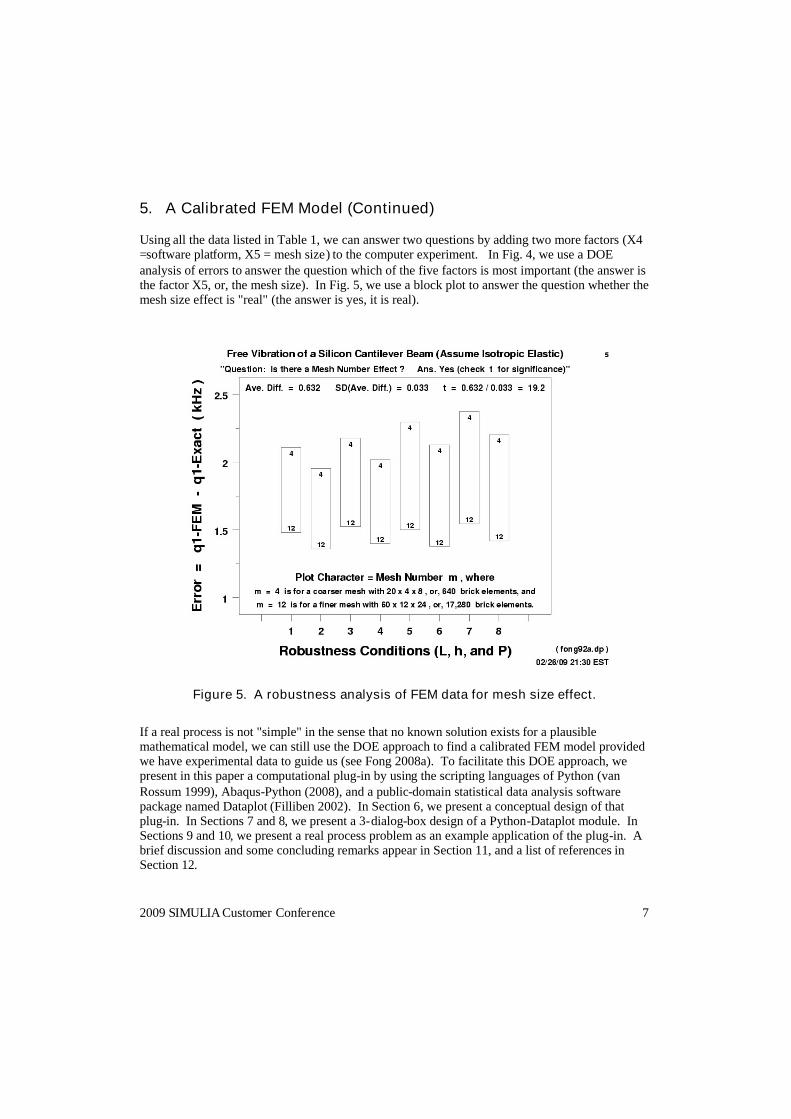
Figure 4. A ranking of five factors based on a DOE analysis of errors.


5. A Calibrated FEM Model (Continued)

Using all the data listed in Table 1, we can answer two questions by adding two more factors (X4=software platform, X5 = mesh size) to the computer experiment. In Fig. 4, we use a DOEanalysis of errors to answer the question which of the five factors is most important (the answer isthe factor X5, or, the mesh size). In Fig. 5, we use a block plot to answer the question whether themesh size effect is "real" (the answer is yes, it is real).

Figure 5. A robustness analysis of FEM data for mesh size effect.

If a real process is not "simple" in the sense that no known solution exists for a plausiblemathematical model, we can still use the DOE approach to find a calibrated FEM model providedwe have experimental data to guide us (see Fong 2008a). To facilitate this DOE approach, wepresent in this paper a computational plug-in by using the scripting languages of Python (vanRossum 1999), Abaqus-Python (2008), and a public-domain statistical data analysis softwarepackage named Dataplot (Filliben 2002). In Section 6, we present a conceptual design of thatplug-in. In Sections 7 and 8, we present a 3-dialog-box design of a Python-Dataplot module. InSections 9 and 10, we present a real process problem as an example application of the plug-in. Abrief discussion and some concluding remarks appear in Section 11, and a list of references inSection 12.


6. A Conceptual Design of a Python-Dataplot Uncertainty Plug-In

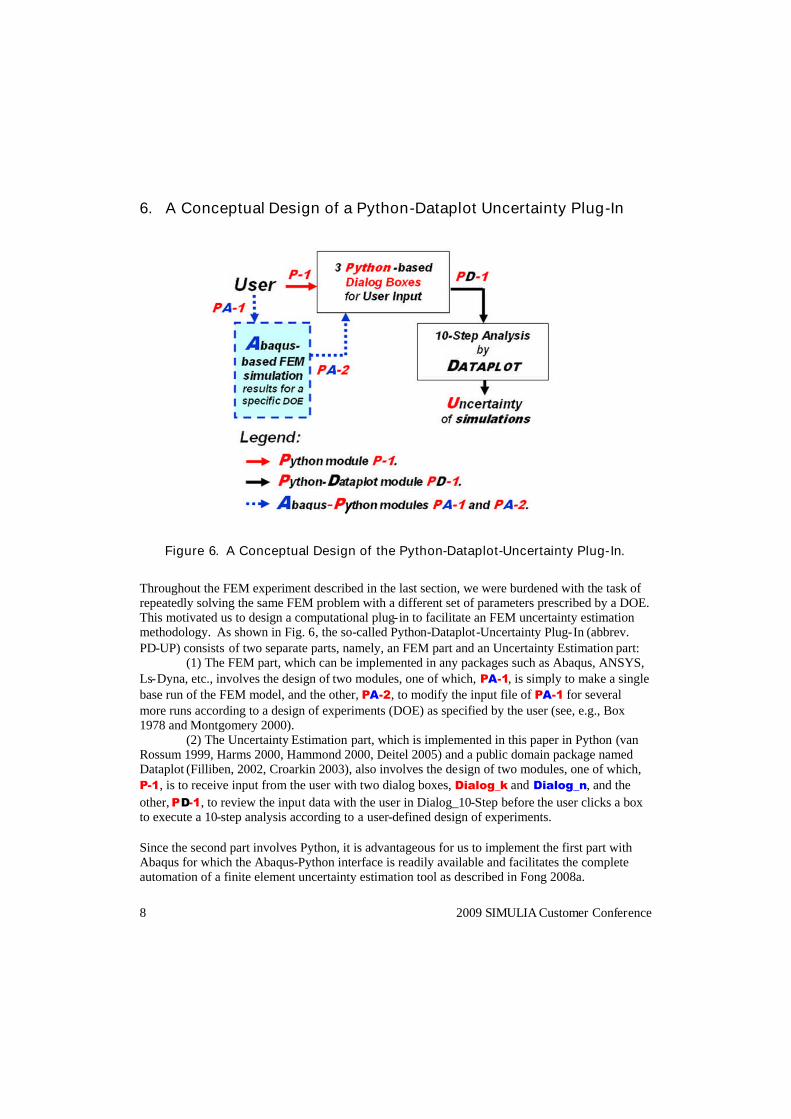
Figure 6. A Conceptual Design of the Python-Dataplot-Uncertainty Plug-In.

Throughout the FEM experiment described in the last section, we were burdened with the task ofrepeatedly solving the same FEM problem with a different set of parameters prescribed by a DOE.This motivated us to design a computational plug-in to facilitate an FEM uncertainty estimationmethodology. As shown in Fig. 6, the so-called Python-Dataplot-Uncertainty Plug-In (abbrev.PD-UP) consists of two separate parts, namely, an FEM part and an Uncertainty Estimation part:

(1) The FEM part, which can be implemented in any packages such as Abaqus, ANSYS,Ls-Dyna, etc., involves the design of two modules, one of which, PA-1, is simply to make a singlebase run of the FEM model, and the other, PA-2, to modify the input file of PA-1 for severalmore runs according to a design of experiments (DOE) as specified by the user (see, e.g., Box1978 and Montgomery 2000).

(2) The Uncertainty Estimation part, which is implemented in this paper in Python (vanRossum 1999, Harms 2000, Hammond 2000, Deitel 2005) and a public domain package namedDataplot (Filliben, 2002, Croarkin 2003), also involves the design of two modules, one of which,P-1, is to receive input from the user with two dialog boxes, Dialog_k and Dialog_n, and theother, PD-1, to review the input data with the user in Dialog_10-Step before the user clicks a boxto execute a 10-step analysis according to a user-defined design of experiments.

Since the second part involves Python, it is advantageous for us to implement the first part withAbaqus for which the Abaqus-Python interface is readily available and facilitates the completeautomation of a finite element uncertainty estimation tool as described in Fong 2008a.


7. A Two-Dialog-Box Design for User's Input Module, P-1

The user's input module, P-1, consists of two dialog boxes, Dialog_k (PyDpGui_1.py) andDialog_n (PyDpGui_2.py). A complete listing of PyDpGui_1.py is given in a website and isdownloadable.

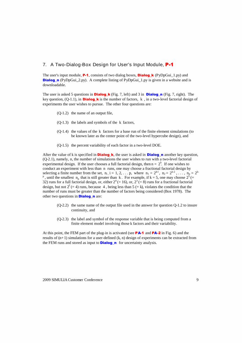
The user is asked 5 questions in Dialog_k (Fig. 7, left) and 3 in Dialog_n (Fig. 7, right). Thekey question, (Q-1.1), in Dialog_k is the number of factors, k , in a two-level factorial design ofexperiments the user wishes to pursue. The other four questions are:

(Q-1.2) the name of an output file,

(Q-1.3) the labels and symbols of the k factors,

(Q-1.4) the values of the k factors for a base run of the finite element simulations (tobe known later as the center point of the two-level hypercube design), and

(Q-1.5) the percent variability of each factor in a two-level DOE.

After the value of k is specified in Dialog_k, the user is asked in Dialog_n another key question,(Q-2.1), namely, n, the number of simulations the user wishes to run with a two-level factorialexperimental design. If the user chooses a full factorial design, then n = 2k. If one wishes toconduct an experiment with less than n runs, one may choose a fractional factorial design byselecting a finite number from the set, ni , i = 1, 2, . . . p, where n1 = 2k-1 , n2 = 2k-2 , . . . , np = 2k-

p , until the smallest np that is still greater than k . For example, if k = 5, one may choose 25 (=32) runs for a full factorial design, or, either 24 (= 16), or, 23 (= 8) runs for a fractional factorialdesign, but not 22 (= 4) runs, because 4 , being less than 5 (= k), violates the condition that thenumber of runs must be greater than the number of factors being considered (Box 1978). Theother two questions in Dialog_n are:

(Q-2.2) the same name of the output file used in the answer for question Q-1.2 to insurecontinuity, and

(Q-2.3) the label and symbol of the response variable that is being computed from afinite element model involving those k factors and their variability.

At this point, the FEM part of the plug-in is activated (see PA-1 and PA-2 in Fig. 6) and theresults of (n+1) simulations for a user-defined (k, n) design of experiments can be extracted fromthe FEM runs and stored as input to Dialog_n for uncertainty analysis.


7. A Two-Dialog-Box Design for User's Input Module, P-1 (Cont'd)

Figure 7. (Left) Dialog_k to define k factors and enter their variability(Right) Dialog_n to choose n runs for a ( k, n ) design and enter results.

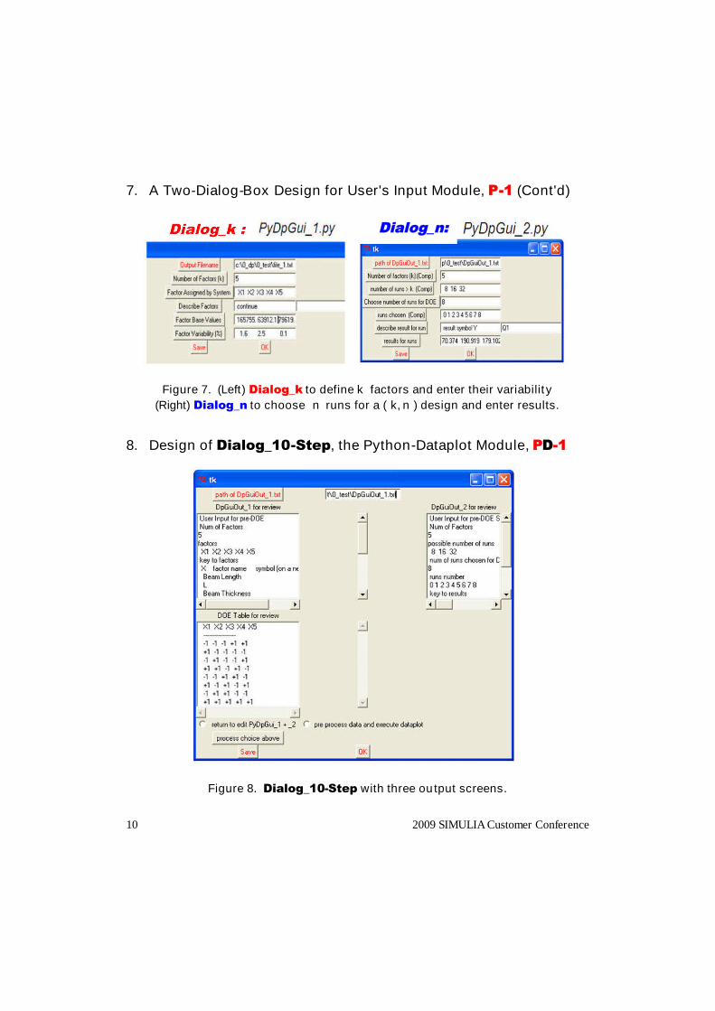
8. Design of Dialog_10-Step, the Python-Dataplot Module, PD-1

Figure 8. Dialog_10-Step with three output screens.

Dialog_n:

2009 SIMULIA Customer Conference11

We are now ready to activate the uncertainty estimation of the PD-UP design by invokingDialog_10-Step (PyDpGui_3.py. See Fig. 8.). The user is first asked to fill in the name of theoutput file specified earlier in Dialog_k. When that name is correct, three screens of input datawill be displayed for review. The first screen (upper left of Fig. 8) is a review of the user's input toDialog_k. The second screen (upper right of Fig 8) is a review of the user's input to Dialog_n.The third screen (lower left of Fig. 8) is new to the user, and contains the DOE table for the valuesof k and n furnished by the user in Dialog_k and Dialog_n.

If the user is not satisfied, the dialog box will return to Dialog_k and Dialog_n. Otherwise, adataplot code named "pedro7.dp" is activated to run the 10-step statistical analysis and return an11-plot file for viewing and downloading. The plot 11 is the uncertainty estimation result such asthose given in Figs. 2 and 3.

9. An Example of an FEM Model without a Known Solution

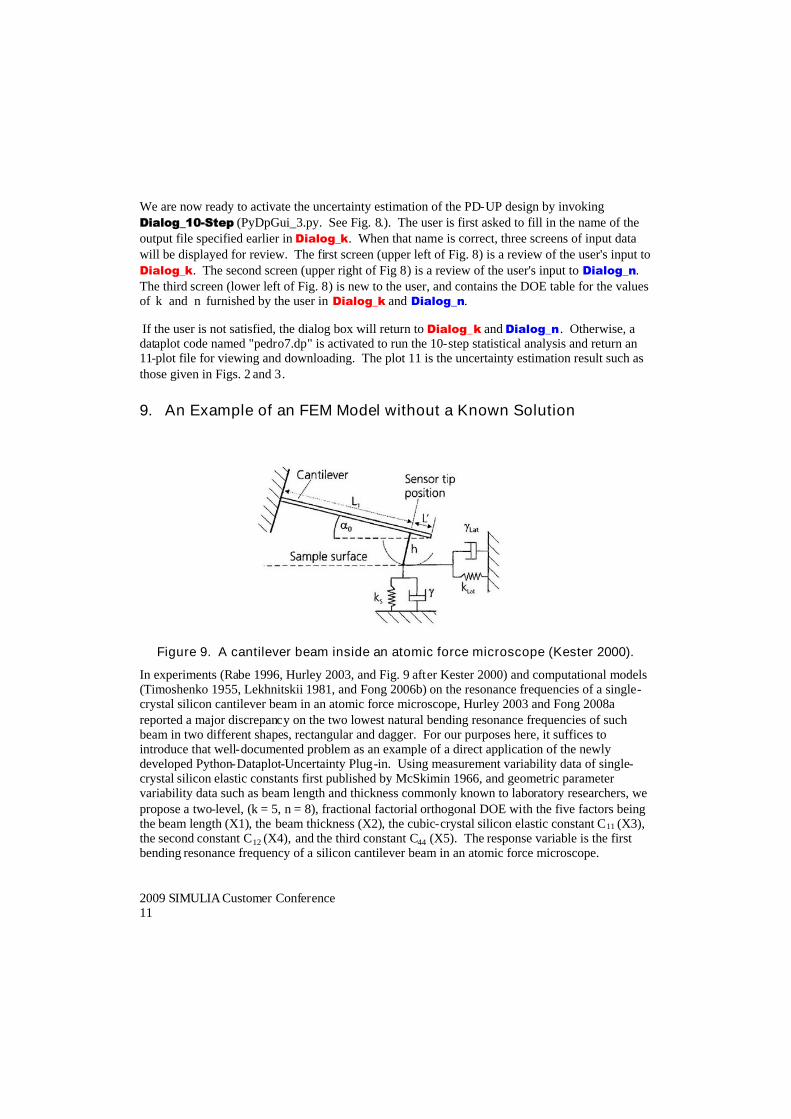
Figure 9. A cantilever beam inside an atomic force microscope (Kester 2000).

In experiments (Rabe 1996, Hurley 2003, and Fig. 9 after Kester 2000) and computational models(Timoshenko 1955, Lekhnitskii 1981, and Fong 2006b) on the resonance frequencies of a single-crystal silicon cantilever beam in an atomic force microscope, Hurley 2003 and Fong 2008areported a major discrepancy on the two lowest natural bending resonance frequencies of suchbeam in two different shapes, rectangular and dagger. For our purposes here, it suffices tointroduce that well-documented problem as an example of a direct application of the newlydeveloped Python-Dataplot-Uncertainty Plug-in. Using measurement variability data of single-crystal silicon elastic constants first published by McSkimin 1966, and geometric parametervariability data such as beam length and thickness commonly known to laboratory researchers, wepropose a two-level, (k = 5, n = 8), fractional factorial orthogonal DOE with the five factors beingthe beam length (X1), the beam thickness (X2), the cubic-crystal silicon elastic constant C11 (X3),the second constant C12 (X4), and the third constant C44 (X5). The response variable is the firstbending resonance frequency of a silicon cantilever beam in an atomic force microscope.


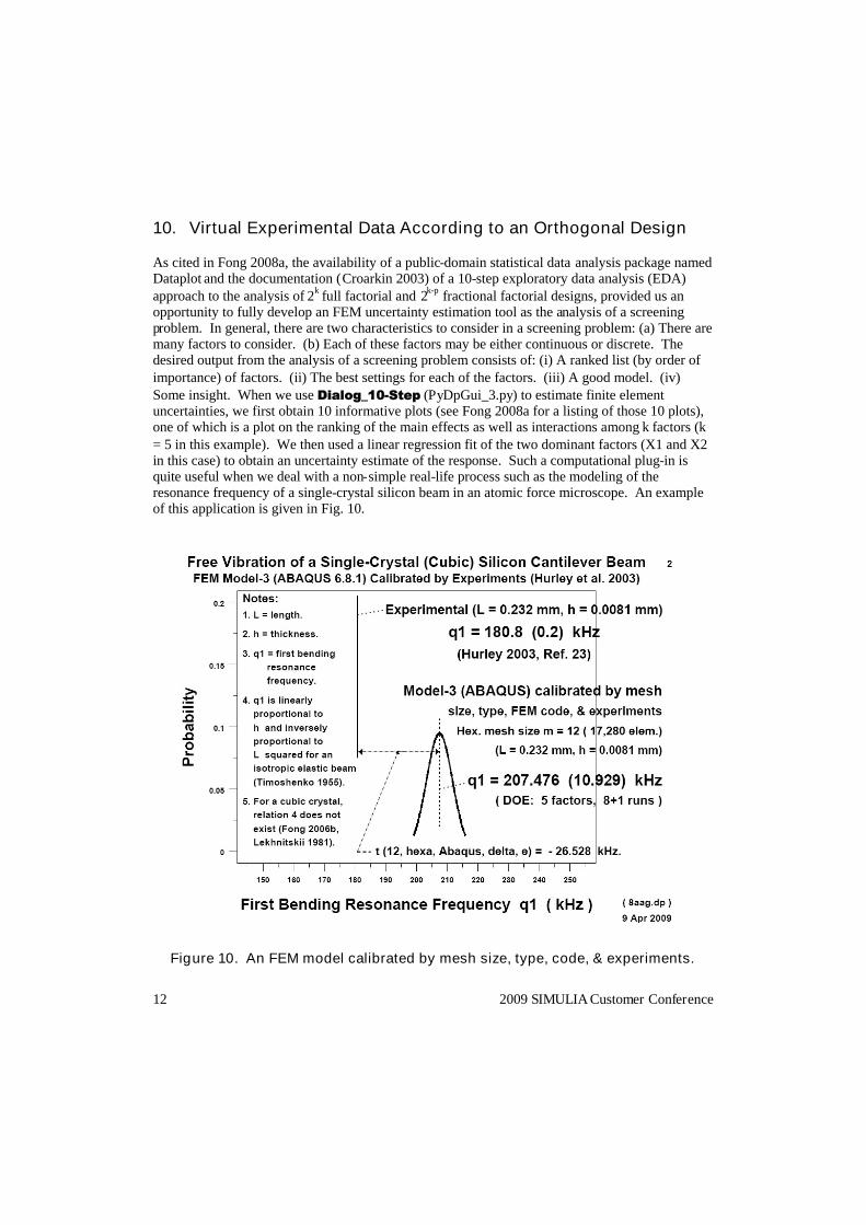
10. Virtual Experimental Data According to an Orthogonal Design

As cited in Fong 2008a, the availability of a public-domain statistical data analysis package namedDataplot and the documentation (Croarkin 2003) of a 10-step exploratory data analysis (EDA)approach to the analysis of 2k full factorial and 2k-p fractional factorial designs, provided us anopportunity to fully develop an FEM uncertainty estimation tool as the analysis of a screeningproblem. In general, there are two characteristics to consider in a screening problem: (a) There aremany factors to consider. (b) Each of these factors may be either continuous or discrete. Thedesired output from the analysis of a screening problem consists of: (i) A ranked list (by order ofimportance) of factors. (ii) The best settings for each of the factors. (iii) A good model. (iv)Some insight. When we use Dialog_10-Step (PyDpGui_3.py) to estimate finite elementuncertainties, we first obtain 10 informative plots (see Fong 2008a for a listing of those 10 plots),one of which is a plot on the ranking of the main effects as well as interactions among k factors (k= 5 in this example). We then used a linear regression fit of the two dominant factors (X1 and X2in this case) to obtain an uncertainty estimate of the response. Such a computational plug-in isquite useful when we deal with a non-simple real-life process such as the modeling of theresonance frequency of a single-crystal silicon beam in an atomic force microscope. An exampleof this application is given in Fig. 10.

Figure 10. An FEM model calibrated by mesh size, type, code, & experiments.


11. Discussion and Concluding Remarks

In this expository paper on a two-part code implementation of a DOE-based FEM uncertaintyestimation methodology, we have presented only the uncertainty estimation part of the plug-in,namely, three Python codes, PyDpGui_1.py, PyDpGui_2.py, and PyDpGui_3.py, and one Dataplotcode, pedro7.dp. All four codes are available at http://math.nist.gov/mcsd/software.html. Wehave left the FEM part open, because our purpose is to make the plug-in, PD-UP (v. 1.0), availablefor any finite element uncertainty estimation effort using either commercially-available,proprietary, or public-domain FEM packages. For instance, when the FEM package is Abaqus,we plan to specialize our PD-UP with a link to Abaqus-Python and name the resulting plug-in theAbaqus-PD-UP. A similar link can be made to another Python-based FEM package namedMPACT, and the resulting plug-in will be named MPACT-PD-UP, and so on. All of the newplug-ins, of course, will be coded in Python.

As illustrated in our numerous examples, we conclude that it is feasible to apply a DOE-basedmethodology to the estimation of FEM uncertainty due not only to model inadequacy, physicalparameters, and observation errors, but also to computer black box parameters such as mesh size,type, and code implementation. Recent FEM simulations with or without using Python as ascripting language (see, e.g., Langer 2001, Easley 2007, Chao 2008, Fong 2008b) and new FEMsimulations such as Fong 2009 may benefit from this plug-in when uncertainty of the computercode vs. real process observations is a compelling issue.

Based on the results presented in Figs. 4 and 5 of Section 5, where we showed two ways ofanswering a question whether a specific factor such as the mesh size has an effect, we observe thatthe computational plug-in, PD-UP, v. 1.0, reported in this paper, is applicable only to theautomation of the 10-step sensitivity and uncertainty analysis of FEM calculations (Fig. 2). Afuture verstion of PD-UP incorporating the block plot methodology (Fig. 5) as well as theremaining FEM part of the plug-in will complete the larger goal of this paper, namely, a cost-effective and user-friendly FEM uncertainty estimation for modeling real processes of multiplefactors.

12. References

1. Abaqus, "Abaqus Scripting User’s Manual, Version 6.8." Dassault Systemes Simulia Corp.,166 Valley Street, Providence, RI, 2008.

2. Abaqus, "Abaqus User’s Manual, Version 6.8.0." Dassault Systemes Simulia Corp., 166Valley Street, Providence, RI, 2008.

3. ANSYS, "ANSYS User’s Manual, Release 11.0." ANSYS, Inc., 275 Technology Dr.,Cannonsburg, PA, 2008.

4. Box, G. E., Hunter, W. G., and Hunter, J. S., "Statistics for Experimenters: An Introduction toDesign, Data Analysis, and Model Building." Wiley (1978).

5. Chao, Y. J., Fong, J. T., and Lam, P. S., "A New Approach to Assessing the Reliability ofApplying Laboratory Fracture Toughness Test Data to Full-Scale Structures," Proc. ASME


Pressure Vessels & Piping Conference, July 27-31, 2008, Chicago, IL, Paper No. PVP2008-61584, http://www.asmeconferences.org/PVP08, 2008.

6. Chu, E., Zhang, L., Wang, S., Zhu, X, and Maker, B., 2002, “Validation of SpringbackPredictability with Experimental Measurements and Die Compensation for AutomotivePanels,” Proc. 5th International Conf. and Workshop on Numerical Simulation of 3-D SheetMetal Forming Processes - Verification of Simulation with Experiment, Jeju Islands, Korea,Oct. 21-25, 2002, Yang, D., Oh, S. I., Huh, H., and Kim, Y. H., eds., Vols. 1. pp. 313-318.Published by the Korean Adv Inst Sci & Tech., 373-1, Science Town, Taejon, 305-701, Korea2002.

7. Clough, R., and Penzien, J., "Dynamics of Structures," 2nd ed. (Revised). Berkeley, CA94704: Computers and Structures, Inc., 2003.

8. Croarkin, C., Guthrie, W., Heckert, N. A., Filliben, J. J., Tobias, P., Prins, J., Zey, C.,Hembree, B., and Trutna, eds., 2003, "NIST/SEMATECH e-Handbook of Statistical Methods,Chapter 5 on Process Improvement (pp. 1-480)," http://www.itl.nist.gov/div898/handbook/,first issued, June 1, 2003, and last updated July 18, 2006. Produced jointly by the StatisticalEngineering Division of the National Institute of Standards & Technology, Gaithersburg, MD,and the Statistical Methods Group of SEMITECH, Austin, TX. Also available as a NISTInteragency Report in a CD-ROM upon request to [email protected], 2006.

9. Deitel, H. M., Deitel, P. J., Liperi, J. P., and Wiedermann, B. A., "Python: How to Program,"first edition. Prentice-Hall, 2005.

10. Draper, N. R., and Smith, H., "Applied Regression Analysis." Wiley (1966).

11. Easley, S., Pal, S., Tomaszewski, P., Petrella, A., Rulkowtter, P., and Laz, P., "FiniteElement-based Probabilistic Analysis Tool for Orthopaedic Applications," Computer Methodsand Programs in Biomedicine, Vol. 85, Issue 1, pp. 32-40, 2007.

12. Filliben, J. J., and Heckert, N. A., "DATAPLOT: A Statistical Data Analysis SoftwareSystem," A Public Domain Software Released by NIST, Gaithersburg, MD 20899,http://www.itl.nist.gov/div898/software/dataplot.html, 2002.

13. Fong, J. T., "ABC of Statistics for Verification and Validation (V&V) of Simulations of High-Consequence Engineering Systems," Proc. 2005 ASME Pressure Vessels and PipingConference, July 17-21, 2005, Denver, CO, Paper No. PVP2005-MF-13-1, 2005.

14. Fong, J. T., Filliben, J. J., deWit, R., Fields, R. J., Bernstein, B., and Marcal, P. V.,"Uncertainty in Finite Element Modeling and Failure Analysis: A Metrology-BasedApproach," ASME Trans., J. Press. Vess. Tech., Vol. 128, pp. 140-147, 2006a.

15. Fong, J. T., Filliben, J. J., deWit, R., and Bernstein, B., "Stochastic Finite Element Method(FEM) and Design of Experiments for Pressure Vessel and Piping (PVP) Decision Making,"Proc. of 2006 ASME Pressure Vessels and Piping Division Conference, July 23-27, 2006,Vancouver, B. C., Canada, paper no. PVP2006-ICPVT11-93927. New York, NY: AmericanSociety of Mechanical Engineers, 2006b.

16. Fong, J. T., Filliben, J. J., Heckert, N. A., and deWit, R., "Design of Experiments Approach toVerification and Uncertainty Estimation of Simulations Based on Finite Element Method,"Proc. Conf. Amer. Soc. for Engineering Education, June 22-25, Pittsburgh, PA, Paper AC2008-2725, 2008a.


17. Fong, J. T., Ranson, W. F., III, Vachon, R. I., and Marcal, P. V., "Structural AgingMonitoring via Web-based Nondestructive Evaluation Technology," Proc. ASME PressureVessels & Piping Conference, July 27-31, 2008, Chicago, IL. Paper No. PVP2008-61607,http://www.asmeconferences.org/PVP08, 2008b.

18. Fong, J. T., deWit, R., Kim, Y. S., Dagalakis, N., Filliben, J. J., and Heckert, N. A., "AMetrological Approach to Comparing Accuracy of Finite Element Software Packages usingTetrahedral vs. Hexahedral Element Meshes," Manuscript in preparation, 2009.

19. Haldar, A., Guran, A., and Ayuub, B. M., eds. "Uncertainty Modeling in Finite Element,Fatigue and Stability of Systems." World Scientific Publishing Co. Pte. Ltd., 1060 MainStreet, River Edge, NJ, 1997.

20. Hammond, M., and Robinson, A., "Python Programming on Win32," O'Reilly Media, Inc.,2000.

21. Harms, D., and McDonald, K., "The Quick Python Book," http://www.manning.com,Manning Pub. Co., 2000.

22. Hughes, T. J. R., "The Finite Element Method: Linear Static and Dynamic Finite ElementAnalysis." Prentice-Hall, 1987.

23. Hurley, D. C., Shen, K., Jennett, N. M., and Turner, J. A., “Atomic force acoustic microscopymethods to determine thin-film elastic properties,” J. Appl. Phys., 94(4), 2347-2354, 2003.

24. ISO, 1993, "Guide to the Expression of Uncertainty in Measurement," Prepared by ISOTechnical advisory Group 4 (TAG 4), Working Group 3 (WG 3), Oct. 1993. ISO/TAG 4,Sponsored by the BIPM (Bureau International des Poids et Mesures), IEC (InternationalElectrotechnical Commission), IFCC (International Federation of Clinical Chemistry), ISO,IUPAC (Int. Union of Pure and Applied Chemistry), IUPAP (International Union of Pure andApplied Physics), and OIML (Int. Organization of Legal Metrology), 1993.

25. Kennedy, M. C., and O'Hagan, A., "Bayesian calibration of computer models," J. RoyalStatistical Soc., Serial B, Vol. 63, Part 3, pp. 425-464 (2001).

26. Kester, E., Rabe, U., Presmanes, L., Tailhades, Ph., and Arnold, W., “Measurement ofYoung’s Modulus of Nanocrystalline Ferrites with Spinel Structures by Atomic ForceAcoustic microscopy,” J. Phys. Chem. Solids, 61, 1275-1284, 2000.

27. Langer, S. A., Fuller, E. R., and Carter, W. C., "OOF: An Image-Based Finite-ElementAnalysis of Material Microstructure," Computing in Science and Engineering, Vol. 3, No. 3,pp. 15-23, May/June 2001.

28. Langtangen, H. P., "Python Scripting for Computational Science," third edition. Springer,2008.

29. Lekhnitskii, S. G., "Theory of Elasticity of an Anisotropic Body," Translated from the revised1977 Russian edition. Moscow: MIR Publishers, 1981.

30. Lord, G. J., and Wright, L., "Uncertainty Evaluation in Continuous Modeling," Report to theNational Measurement System Policy Unit, Department of Trade and Industry, NPL ReportCMSC 31/03. Teddington, Middlesex, U.K.: National Physical Laboratory, 2003.

31. LSTC, "Ls-Dyna Keyword User’s Manual, Version 970," April 2003, Livermore SoftwareTechnology Corp., Livermore, CA, 2003.


32. Marcal, P. V., "MPACT User's Manual." Published by MPACT Corp., Julian CA,[email protected], 2008.

33. McSkimin, H. J., and Andreatch, P., Jr., “Elastic Moduli of Silicon vs. Hydrostatic Pressure at25.0 C and - 195.8 C,” J. Appl. Phys., 35(7), 2161-2165, 1964.

34. Montgomery, D. C., "Design and Analysis of Experiments," 5th ed. Wiley, 2000.

35. Rabe, U., Janser, K., and Arnold, W., “Vibrations of free and surface-coupled atomic forcemicroscope cantilevers: Theory and experiment,” Rev. Sci. Instrum., 67 (9), 3281-3293, 1996.

36. Taylor, B. N., and Kuyatt, C. E., "Guidelines for Evaluating and Expressing the Uncertaintyof NIST Measurement Results," NIST Tech. Note 1297, Sep. 1994 edition (supersedes Jan.1993 edition), Prepared under the auspices of the NIST Ad Hoc Committee on UncertaintyStatements, U. S. Government Printing Office, Washington, DC, 1994.

37. Timoshenko, S., and Young, D. H., "Vibration Problems in Engineering," 3rd ed. D. VanNostrand, 1955.

38. van Rossum, G., "Python Tutorial," Feb. 19, 1999, Release 1.5.2. Corp. for NationalResearch Initiative (CNRI), 1895 Preston White Dr., Reston, VA, 1999.

39. Yang, D., Oh, S. L., Huh, H., and Kim, Y. H., eds., “Numisheet 2002: Design InnovationThrough Virtual Manufacturing,” Proc. 5th Int. Conf. and Workshop on NumericalSimulation of 3D Sheet Forming Processes - Verification of Simulation with Experiment, 21–25 October 2002, Jeju Island, Korea, Vol. 2, published by Korean Adv Inst Sci & Tech., 373-1, Science Town, Taejon, 305-701, Korea, 2002.

40. Zienkiewicz, O. C., and Taylor, R. L., "The Finite Element Method," 5th ed., Vol. 1, TheBasis. Butterworth-Heinemann, 2000.

13. Acknowledgment

We wish to thank Ron Boisvert, Andrew Dienstfrey, and Alden Dima, all of NIST, AndrewMacKeith and David C. Winkler of Dassault Systemes Simulia Corp., Providence, RI, and RobertRainsberger of XYZ Scientific Applications, Inc., Livermore, CA, for their technicaldiscussions/comments during the course of this investigation.

14. Disclaimer

The views expressed in this paper are strictly those of the authors and do not necessarily reflectthose of their affiliated institutions. The mention of the names of all commercial vendors and theirproducts is intended to illustrate the capabilities of existing products, and should not be construedas endorsement by the authors or their affiliated institutions.

Documents

A Design-of-Experiments Plug-In for Estimating Uncertainties in Finite Element Simulations · 2009-10-26 · A Design-of-Experiments Plug-In for Estimating Uncertainties in Finite