A Data Mining Approach to Validating Drillhole Logging

Data in Pilbara Iron Ore Exploration

Daniel Wedge1, Andrew Lewan2, Mark Paine2, Eun-Jung Holden1 and Thomas

Green2 1Centre for Exploration Targeting, The University of Western Australia, Crawley WA 6009, Australia

2Rio Tinto Iron Ore, 152-158 St Georges Terrace, Perth WA 6000, Australia

Abstract

Logging of exploration drillholes is a routine practice and its accuracy is essential for

resource evaluation and planning in the minerals industry. Logged compositions record a set of

material types with standardized mineralogy and texture characteristics. The material types logged

may vary due to diversities in mineralization and geology, but also due to subjective biases and

human error, leading to significant challenges for the industry. Thus, there is a need to validate the

field logging whereby the material types and their percentages are adjusted to reconcile with

laboratory assay values, while retaining the physical characteristics and geological context.

We introduce the Auto-Validation Assistant (AVA) algorithm that applies data mining

methods to geologists’ validation patterns recorded in a training process over hundreds of intervals of

iron ore exploration drillholes. The AVA modifies the material types selected in the logged

composition and their percentages according to geological rules learned in the training process, and

proposes to the geologist a number of validated compositions with optimized geochemistry and

mineralogical hardness, while also considering visible properties such as chip shape and color. Using

the confidence value provided with each validated composition, the geologist can make informed

validation decisions and remains in control of the validation process, while harnessing computational

power.

Experiments were conducted to evaluate the auto-validated compositions generated by AVA:

one to analyze the acceptance rate of the AVA generated compositions by geologists for 1,996

intervals in drillholes from different sites; and the other to compare manual and AVA-validated

compositions using 14,600 drillholes from one entire deposit. The results showed the acceptance rate

of AVA-validated compositions (without further change) of 74.3%, leading to significant time savings

over tedious manual validation, while demonstrating that AVA provides comparable but more

consistent results. The algorithm is fast and repeatable and can be adapted to different material types

and training datasets, with potential applications beyond iron ore exploration.

Introduction Rock samples from drillhole data provide mineralogical details crucial for orebody modeling

and mining. A conventional mining exploration process involves drilling, logging and assaying

exploration holes to better understand the structures and mineralogical compositions of an area

(Sommerville et al., 2014). The modeled orebody volume, shape and grade form the basis of resource

estimation block models for mining and planning purposes. However, drillhole logging is challenging

due to the visual and textural ambiguity of some mineralogical types in small chip samples. Thus, the

logging heavily relies on geologists’ ability and subjective biases, which leads to variable outcomes.

Incorrect drillhole logging can result in outcomes with significant financial implications. In

particular, in iron ore exploration and mining, ochreous goethite material and shale are commonly

confused due to similarities in color and texture in chip samples obtained from reverse circulation

(RC) drilling. However, these types are chemically very different, shale that is enriched in kaolinite is

high in silica and alumina and low in iron, whereas ochreous goethite has a high iron grade but is

much lower in silica and alumina than shale. Another property of ochreous goethite is its water

holding capacity due to high levels of microporosity (Paine et al., 2016). As a result, it is sticky and

causes problems such as blocking screen decks as shown in Figure 1, and ore transfer chutes, leading

to unplanned downtime. Thus, there is a need to validate the logging data in order to improve the

robustness of resource estimates, and provide more accurate knowledge of the distribution of

ochreous goethite which can assist in planning blending strategies to manage risks in mining.

Figure 1: Accurate modeling of ochreous goethite is necessary to prevent handling problems such as this

blocked screen. From Paine et al. (2016).

Given that the logged composition summarizes the interval as percentages of material types,

each type having average theoretical assay values, the interval’s theoretical assays can be estimated

from the logging. Validation involves adjusting the percentages of the logged material types, and

adding or removing material types where necessary using geologically informed substitutions so that

the theoretical assay values are within an error tolerance of the laboratory assay values obtained from

the interval’s chip samples. Error tolerances are used here not only as a measure of logging error, but

also to allow for variability in the chemistry within each material type. To mitigate these variations,

theoretical assays for each material type are maintained independently from site to site, and their

values are routinely updated via reconciliation against plant data. Mineralized material types exhibit

only small variations in Fe grade of up to 5%, though for most mineralized types the variation is less

than 2%. Other material types may exhibit more variation though for product grade prediction, this is

not a concern because waste material corresponding to these types is not typically processed through

the plant.

In the following sections, we discuss logging and validation, the process of applying machine

learning to recorded validation data, and deriving geologically feasible combinations of material

types. Then we introduce the Auto-Validation Assistant (AVA) algorithm, which utilizes this training

data and exploits computational power to explore a large space of possible solutions, of which a small

number are proposed to the geologist. Finally we evaluate AVA on iron ore exploration projects in the

Hamersley province in Western Australia.

Logging and Validation

RC drilling produces chip samples from which the logged compositions are estimated. Chip

samples for each 2m interval are brought to the surface, and a rotary cone splitter used to divide the

chips into equally distributed samples. Chips from one sample are logged by scooping a cup of

material from the slurry, passing it through a sieve and estimating (1) the percentages of various

material types present in the sieve (usually in increments of 5%), (2) the sample color, (3) the chips’

shape, and (4) the recovered percentage (Sommerville et al., 2014). The other sample is sent for

laboratory XRF assay analysis, to measure Fe, SiO2, Al2O3, P, S, Mn, MgO, TiO2, CaO, Total LOI,

LOI425 (typically indicating goethite-bound water) and LOI650 (typically indicating kaolinite

associated water) measurements. Total Fe and Mn values are reported rather than their oxides due to

their different possible oxidation levels. Additionally, using total Fe provides consistency with Fe

units used elsewhere in resource estimation.

A logged composition for each 2m interval estimates the percentages of the interval’s chips in

terms of material types. The Material Type Classification Scheme (MTCS; Box et al., 2002) was

developed to standardize primary characteristics, such as mineralogy and texture, in a hierarchical

manner. It models physical and chemical attributes to predict metallurgical behavior and product

quality for optimal ore processing (Paine et al., 2016). Each material type has theoretical assay,

hardness, and lump-fine splits corresponding to particles larger or smaller than 6.3mm, with

corresponding lump-fine geochemistry differences, thus enabling downstream estimation of a

theoretical assay value, as well as lump-fine splits and handling characteristics of an orebody.

Material types have been defined to be identifiable at scales ranging from microscopic (polished

block) to macroscopic (chips, hand specimen and face scales). These qualitative physical properties

remain consistent from site to site, though minor changes in geochemistry and physical properties

such as lump % may occur. Some selected material types are listed in Error! Reference source not

found..

Goethite dominant mineralogy

GOE Earthy goethite

GOL Ochreous goethite

GOV Vitreous goethite

Hematite goethite mineralogy

H2F Microplaty hematite + martite (friable)

H2H Microplaty hematite + martite (hard)

H2M Microplaty hematite + martite (medium)

Hematite dominant mineralogy

HGF Martite-ochreous goethite + goethite

HGM Martite ± microplaty hematite + goethite

HGH Martite-vitreous goethite + goethite

Selected waste lithology codes

SHL Shale

SID Siderite

BIF Banded iron formation (waste)

CAL Calcrete

CHT Chert

CLA Clay Table 1: A subset of commonly-used codes from the MTCS

During validation, the logged composition is adjusted to match the assay values using

geologically informed addition or removal of material types and adjusting their percentages, resulting

in a validated composition. Validation cannot be performed in a vacuum; the original field logging

provides an important source of information and must be used to inform the validation. In validation,

there must be some common thread linking the interchanged material types. For example, two types

may be swapped if they share similar physical characteristics, but significantly different chemistry.

Some material types are physically distinctive and their presence is obvious, including pisolite. The

percentages of these logged types may be altered within a logging error bound, but the type should

never be removed or added. Thus validation is not just a goal-seeking exercise to minimize the assay

error; a number of geological and physical constraints must also be satisfied. The validation process is

summarized in Figure 2.

Figure 2: The relationships between validation and the logged and validated compositions.

Validation is time consuming, laborious and often inconsistent between geologists. On

average, each 2m interval of an RC hole takes a number of minutes to validate. As hundreds of

kilometers of RC holes are drilled each year by Rio Tinto Iron Ore in the Pilbara (Sommerville et al.,

2014), it is therefore an extremely labor intensive task.

Data Mining of Validation Patterns

To understand geologists’ validation patterns and provide training data for our algorithm, 11

experienced geologists were recorded performing validation. Data was collected through validation of

6 holes: 3 holes from one site and 3 from a second site, from iron ore deposits within the Marra

Mamba formation and Brockman Iron Formation in the Hamersley Province. The Marra Mamba

Formation is a banded iron formation (BIF) structure interleaved with shale bands (Trendall and

Blockley, 1970). It is overlain by the Wittenoom Formation (Trendall and Blockley, 1970) which

consists of dolomite, chert and shale. The Wittenoom Formation itself is overlain by the Mount Sylvia

Formation, the Mount McRae Shale, and then the Brockman Iron Formation, which is another BIF

structure interleaved with shale bands. The Brockman Iron Formation itself comprises the Dales

Gorge Member, overlain by the Whaleback Shale, which itself is overlain by the Joffre Member

(Trendall and Blockley, 1970). Hamersley Detrital deposits, located further up the stratigraphic

sequence, are derived from weathered bedded ores (Morris, 1994).

Each hole was logged by a different field geologist. This provided different sources of error,

reflecting geologists’ varied training and biases. A further 20 standard intervals were validated, in

which theoretical assays were computed from known material type combinations and provided

alongside plausible but deliberately incorrect logging for the user to validate. The geologists validated

4,520 intervals in total.

Step-by-step changes from the logged to the validated compositions were recorded where for

each step, validators swapped some percentage of one material type directly for another material type

with similar physical characteristics, while reducing the total assay error. This allowed the

incremental improvements to be captured, between the logged composition and the validated

composition for each interval. At each step, we recorded the difference between the theoretical assay

value and the actual laboratory assay value (i.e. assay error), along with the material types swapped by

the validator. The assay error is a 12-element vector, one component per element in the assay suite.

Normalization was applied by dividing the vector by the maximum magnitude element so all elements

have values between -1 and 1 (inclusive), then each element was rounded to the nearest 0.2, giving a

normalized assay error. This produced a set of validation rules, where for a given normalized assay

error, some percentage of one material type was removed and the same percentage of another material

type added (which we term the material type swap).

We built a database of validation rules where each rule comprises the normalized assay error,

the material type with increased percentage, the material type with reduced percentage, and the

stratigraphic class containing the training interval. Each validation rule has a weight based on the

percentage change in composition. Rules with identical keys were combined by summing the weights

of the individual rules, thus repeated observations of a rule increase its weight. Rounding the

normalized assay error vector increases the likelihood of rules being merged, reducing the size of the

database. While this causes a minor inaccuracy in the calculation of the angle, described later,

between the actual assay error vector of a composition and the normalized assay error, it is offset by

reducing the number of very similar database rules through which to search, and the resulting states

resulting from applying the same material type swaps with slightly different normalized assay errors

would eventually be identified and merged by the algorithm.

We used three stratigraphic classes: detrital deposits, mineralized bedded, and shales. These

respectively correspond to the: Hamersley detritals; mineralized Marra Mamba and mineralized

Brockman; and BIF shale bands and Wittenoom Formation intervals in our training data. The rules are

partitioned into different stratigraphic classes as some material type swaps will be confined to a

specific class. For example, ochreous goethite is commonly swapped for clay in detritals, but is

geologically unusual elsewhere as one would instead substitute ochreous goethite for shale. This

partitioning also allows us to assign different weights to the same swap with the same assay error in

different strata.

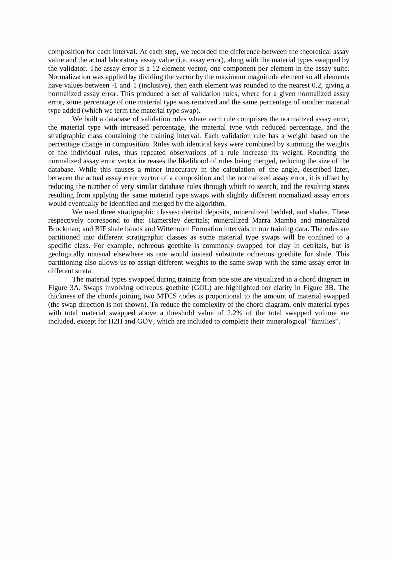
The material types swapped during training from one site are visualized in a chord diagram in

Figure 3A. Swaps involving ochreous goethite (GOL) are highlighted for clarity in Figure 3B. The

thickness of the chords joining two MTCS codes is proportional to the amount of material swapped

(the swap direction is not shown). To reduce the complexity of the chord diagram, only material types

with total material swapped above a threshold value of 2.2% of the total swapped volume are

included, except for H2H and GOV, which are included to complete their mineralogical “families”.

(A) (B)

Figure 3: (A) Material type swaps observed in intervals from one site. (B) Highlighting the swaps involving

ochreous goethite. Descriptions for the MTCS codes are given in Table 1.

The chord diagrams show that the dominant material type swaps are GOE-HGM, SHL-HGF,

GOL-SHL, and GOL-HGF. These findings agree qualitatively with common knowledge, and allow

the magnitudes of these changes to be quantified. For example, during the validation process, GOE

may be removed for HGM (containing some hematite) if a higher theoretical Fe grade and lower

LOI425 value is necessary to match the laboratory assay values. Physically, they are both of medium

hardness and have lower lump characteristics, which is why GOE is preferentially interchanged with

HGM instead of a harder type such as HGH. GOL and HGF are interchanged for similar reasons. SHL

and GOL are easily confused in logging as they share similar physical characteristics, being soft and

yellow, yet chemically they are very different: SHL represents kaolinite high in SiO2, Al2O3 and

LOI650 and low in Fe, whereas GOL is predominantly goethite with a moderately high Fe grade and

has a high LOI425 value.

While the validation rules record which material types were swapped, we also learn which

material types were commonly logged in conjunction with other types to understand the geological

context of the material types. We adapted and extended a method known as the Apriori algorithm

(Agrawal and Srikant, 1994) to determine association rules, whereby logging a set of, or individual,

material types X leads to another material type Y being included in the same composition. Each

association rule has confidence value, defined as the percentage of compositions containing X that

also contain Y. The support for an association rule is defined as the percentage of compositions

containing both X and Y.

The dataset that we used as input for the Apriori algorithm included over 60,000 intervals

each with logged and validated compositions. This was far larger than the dataset used to form the

database of the validation rules, since only the logged and validated compositions are required (i.e.

not the individual swaps made during validation). We ran the Apriori algorithm independently for

intervals from each of the three stratigraphic classes, since geological rules may vary according to

stratigraphy. For example, kaolinite should be logged as the clay MTCS type in detritals, but as the

shale type elsewhere. These patterns are implied in the outputs. We mined association rules with a

minimum support value of 0.1% (per stratigraphy) and a minimum confidence value of 0.1% to

identify only significant trends in compositions.

From these association rules, a set of material type compositions was generated where each

composition was formed from the union of the material types in X and Y. This is for the purpose of

creating a list of subsets of geologically valid material types. Error! Reference source not found.

shows the most common subsets of material types in each stratigraphic class.

Goethite dominant mineralogy

GOE Earthy goethite

GOL Ochreous goethite

GOV Vitreous goethite

Hematite goethite mineralogy

H2F Microplaty hematite + martite (friable)

H2H Microplaty hematite + martite (hard)

H2M Microplaty hematite + martite (medium)

Hematite dominant mineralogy

HGF Martite-ochreous goethite + goethite

HGM Martite ± microplaty hematite + goethite

HGH Martite-vitreous goethite + goethite

Selected waste lithology codes

SHL Shale

SID Siderite

BIF Banded iron formation (waste)

CAL Calcrete

CHT Chert

CLA Clay Table 2: Observed commonly co-logged subsets of material types

The common presence of clay in detrital intervals, high grade hematite and goethite types in

mineralized bedded intervals, and shale in shale intervals is expected. While the data collected

through these steps provides some insights into the validation process and geological context of

material types, it more importantly forms the training data for our algorithm.

Auto-Validation Assistant (AVA) The AVA algorithm mimics the human validation process while exploiting computational

power. It applies material type swaps from the training data collection phase and geological rules

mined by the Apriori algorithm to produce geologically plausible validated compositions with

theoretical assay values closely matching the laboratory assay values. The algorithm’s outputs are

auditable, and training rules can be updated easily without requiring reprocessing all of the training

data. A set of proposed validated compositions are presented, from which users can select what they

judge as the best result. A geologist can also modify the proposed result by adding or removing

material types, and modifying the percentages. Thus, geologists’ knowledge and experience still play

a crucial role in validation. The algorithm’s name implies that it assists the user, while the geologist is

still in control of the final validated composition, rather than being fully automated.

A geologist iteratively applies material type swaps to the logged composition to produce a

validated composition. Although there is no limit to the number of swaps, a median of three swaps

was observed. The AVA algorithm is a parallel version of this framework and the overview is shown

in Figure 4. A swap selection process determines how to apply the training data to the logged

composition. Swaps are applied in parallel and produce numerous parallel intermediate states in each

iteration. An optimization is applied to each intermediate state to select the percentages for each

selected material type to minimize a cost quantifying the differences in the assay and hardness values.

These steps are described in detail below. The cost is used to rank the intermediate states. The best-

ranked intermediate states are selected and the process repeated beginning with the intermediate states

in place of the logged composition. A tree of compositions is therefore created, stemming from the

logged composition. We used 40 intermediate states, and five iterations. These values were selected

empirically as a trade-off between accuracy and time; these parameters acceptable results within five

seconds, and 96% of manual validations during training required five or fewer material type swaps. A

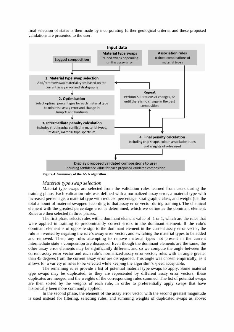
final selection of states is then made by incorporating further geological criteria, and these proposed

validations are presented to the user.

Figure 4: Summary of the AVA algorithm.

Material type swap selection Material type swaps are selected from the validation rules learned from users during the

training phase. Each validation rule was defined with a normalized assay error, a material type with

increased percentage, a material type with reduced percentage, stratigraphic class, and weight (i.e. the

total amount of material swapped according to that assay error vector during training). The chemical

element with the greatest percentage error is determined, which we define as the dominant element.

Rules are then selected in three phases.

The first phase selects rules with a dominant element value of -1 or 1, which are the rules that

were applied in training to predominantly correct errors in the dominant element. If the rule’s

dominant element is of opposite sign to the dominant element in the current assay error vector, the

rule is inverted by negating the rule’s assay error vector, and switching the material types to be added

and removed. Then, any rules attempting to remove material types not present in the current

intermediate state’s composition are discarded. Even though the dominant elements are the same, the

other assay error elements may be significantly different, and so we compute the angle between the

current assay error vector and each rule’s normalized assay error vector; rules with an angle greater

than 45 degrees from the current assay error are disregarded. This angle was chosen empirically, as it

allows for a variety of rules to be selected while keeping the algorithm’s speed acceptable.

The remaining rules provide a list of potential material type swaps to apply. Some material

type swaps may be duplicated, as they are represented by different assay error vectors; these

duplicates are merged and the weights of the corresponding rules summed. The list of potential swaps

are then sorted by the weights of each rule, in order to preferentially apply swaps that have

historically been more commonly applied.

In the second phase, the element of the assay error vector with the second greatest magnitude

is used instead for filtering, selecting rules, and summing weights of duplicated swaps as above;

finally the third greatest magnitude element of the assay error vector is used similarly in the third

phase. Using the three largest elements provides robustness to errors, and allows the algorithm to

select rules that are optimal for three dominant elements to provide a better overall solution within a

reasonable computational time.

In addition, for some dominant elements, manually crafted rules are added for specific

material types related to that element, as these scenarios may have occurred infrequently in the

training dataset. For example, if the theoretical alumina value needs to be increased but not the silica

value, add the gibbsite and/or aluminous goethite material type. There are 15 rules, covering the trace

elements CaO, MgO, Mn, P and S, in each of the three stratigraphic classes.

The material type swaps are applied in parallel, thus the selected intermediate states branch-

out to multiple child states, each with a unique set of material types. At this stage, only the set of

present material types is altered – the actual percentages of each type are determined in the

optimization step. Note that if altering the composition would result in the set of material types

matching those of a composition from an earlier state, the state is discarded to avoid revisiting a

previously processed state.

Optimization The percentages for each material type are calculated by minimizing a cost function that

incorporates three aspects: assay errors, changes in mineral hardness, and changes in lump percentage.

We now discuss the cost function components and constraints before describing the optimization

method details.

Assay errors: We define assay errors in terms of an assay error tolerance factor, which is the

proportion of the assay percentage error relative to a predetermined tolerance value for each element;

a tolerance factor of 1 therefore represents the largest allowable absolute error for that element. The

tolerances are set independently for each element and may vary from project to project according to

requirements, or according to the interval’s iron grade, as less accurate validation is required for low-

grade (waste) intervals. Typically the tolerances in the assay error for Fe and SiO2 are 2.5%, for Al2O3

2%, and the total LOI tolerance is 1.5%. All solutions having theoretical assay values within the

respective tolerance of the laboratory assay value are considered equally valid. Assay error tolerance

factors less than 0.5 are rounded to 0.5 to avoid over-optimization, since material type percentages are

generally presented to the user as integer values for simplicity.

Mathematically, for assay element a, laboratory assay value L, theoretical assay value T, error

tolerance ε, and tolerance factor weighting f, the assay error component Eassay is given by:

𝐸𝑎𝑠𝑠𝑎𝑦 = ∑max(|𝐿𝑎 − 𝑇𝑎|, εa/2)

εa∗ 𝑓𝑎

𝑎

where f=2 for Fe, SiO2 and Al2O3 and 1 otherwise, emphasizing the relative significance of errors in

these elements, and the max(,) function returns the maximum value of the two arguments.

Changes in mineral hardness: The mineral hardness component aims to preserve the logged

composition’s distribution of RC chip hardness, divided into three hardness bins comprising hard,

medium and friable material types. The intermediate state’s composition is partitioned similarly. The

differences of corresponding bin values are taken, minus a grace change in hardness of 10% allowing

for minor changes in hardness without penalty. A change in hardness Δh is computed over Hard,

Medium and Friable bin indices b within the logged composition Blogged and optimized composition

Boptimized:

Δℎ = ∑ max (|𝐵𝑙𝑜𝑔𝑔𝑒𝑑𝑏 − 𝐵𝑜𝑝𝑡𝑖𝑚𝑖𝑧𝑒𝑑

𝑏 | − 0.1, 0)

𝑏∈{𝐻,𝑀,𝐹}

,

where the max function prevents negative values after subtracting the grace change in hardness. The

hardness error component Ehardness is given using a Gaussian function:

𝐸ℎ𝑎𝑟𝑑𝑛𝑒𝑠𝑠 = exp(−Δℎ

2

0.3 ∗ 0.252),

where the constant term 0.3 to adjust the weighting was determined empirically, and the standard

deviation value of 0.25 was derived from the training data.

Changes in lump percentage: The lump percentage for each material type measures the breakdown

into lump (nominally particles >6.3mm or 0.25” in diameter) and fines products. Although the

hardness in the logged data is a qualitative material property, the lump percentage gives a quantitative

measure. Importantly, the grades of the same material type can vary for the resulting lump and fines

product (typically the Fe grade is higher for lump product). Since lump and fines products are

marketed separately, these changes are significant. We aim to match the theoretical lump percent for

the intermediate state to that of the logged composition. A sigmoid function is used to calculate a

lump error component Elump from the change in the lump percentage Δl:

𝐸𝑙𝑢𝑚𝑝 = 0.5 + 1

2 + (Δ𝑙50

)2

The denominator of 50 in the squared term controls the dropoff rate of the error value. The

result ranges from 2/3 (when Δl is at its maximum value of 100) to a maximum of 1 (when Δl = 0).

Optimization algorithm: The cost function is defined using assay errors, Eassay, changes in mineral

hardness, Ehardness, and changes in lump percentage, Elump :

𝐸𝑡𝑜𝑡𝑎𝑙 =𝐸𝑎𝑠𝑠𝑎𝑦 ∗ 𝐸ℎ𝑎𝑟𝑑𝑛𝑒𝑠𝑠

𝐸𝑙𝑢𝑚𝑝∗ (1 + 𝑛)

where n is the number of assay elements with errors greater than that element’s tolerance.

The optimization function uses boundary and linear equality constraints and is implemented

by the optimization package ALGLIB (http://www.alglib.net, Sergey Bochkanov). The boundary

constraints ensure that each material type’s percentage lies between 0 and the maximum value that

would cause the theoretical value for any element to exceed the laboratory assay value by the error

tolerance. Further bounds are applied to specific material types identified as textural types such as

pisolite, where only a small variation in percentage is allowed, for example, ± 10%, as well as

ensuring that the type should not be removed entirely (if less than 10% is logged). Textural types are

rarely confused with other types, and so the field geologist’s logging should not be significantly

modified. Finally, a linear constraint ensures that the material types’ percentages sum to 100%.

The optimization process converges to a local minimum of the cost function given the

constraints. Due to the wide variations in possible optimization constraints and theoretical assay

compositions, we are unable to prove analytically that a global minimum is located, though in

practice, we have observed that a wide range of initial starting parameters converge to the same local

minimum. Therefore, when applying the validation rules, we do not need to directly swap a given

percentage of material type 1 for the same percentage of material type 2; the optimization function

calculates the percentages for the new set of material types that best fit the laboratory assays, hardness

distribution, and the lump percentage.

Intermediate state penalty calculation The intermediate state penalty is applied to each intermediate state to penalize geologically

unusual combinations of material types. It is a numeric multiplier applied to the state’s cost value.

Since it is only dependent on the set of material types (not the percentages) it can be computed after

the optimization for each composition, rather than inside every calculation of the cost function. Large

penalty multipliers (such as 4 or 8) have been used so that an assay match must be significantly better

to counteract the geological penalty. Several geological characteristics are considered, and where the

same characteristic is violated multiple times, penalties are applied repeatedly for each violation

within each intermediate state. Penalties do not accumulate between successive intermediate states.

Stratigraphy: Material type swap rules are applied preferentially from the same stratigraphic class as

the interval being validated by applying a penalty to rules trained from other stratigraphies. For

training rules from a different stratigraphy, we apply a penalty rather than banning them altogether in

order to broaden the set of possible rules, particularly when there are few rules with similar assay

errors to the current state. If a rule introduces a material type that is prohibited in a particular

stratigraphy, the geological inconsistency will be detected by one of the following penalties. It is

important to note that the stratigraphic class may be incorrectly logged, in which case this penalty will

still apply, however applying a penalty is preferable to only selecting rules from within only the

selected stratigraphy. Further, in the majority of intervals where the stratigraphy is correctly logged,

this penalty results in the selection of more appropriate rules.

Conflicting and prohibited material types: Some material type combinations are geologically

forbidden. For example, the MTCS contains three silica material types for different geological

scenarios: the quartz and secondary silica types indicate hydration, and are used in detrital strata, and

to mark faults, whereas the chert type is only used in unhydrated bedded strata. Although chemically

identical for matching assay values and grade estimation, using the wrong type may lead to geological

misunderstandings during modeling; applying a penalty prevents these situations. Similarly, kaolinite

is logged as the clay type in hydrated and detrital intervals, but as the shale type in un-hydrated

intervals. We also apply a penalty for combining end member material types predominantly consisting

of one element. For example, using gibbsite (alumina) together with quartz (silica), in place of a

kaolinite type which is high in both elements and is more likely geologically.

Texture: Some material types have distinctive textures and their presence is obvious. If one of these

types is logged, a penalty is applied if the type is completely removed during validation. A penalty is

also applied for adding one of these material types if not originally logged.

Hydration: Some material types, such as vitreous goethite, have characteristics arising from hydration

and should only be included if the interval is in a known hydrated zone. Conversely, some material

types are less common in the hydrated zone, such as the chert and shale types. We apply penalties for

using hydrated types in non-hydrated intervals or vice-versa. Even though LOI is indicative of

hydration, some types are a by-product of hydration and will not have any LOI signature, for example

precipitated silica. Additionally, while some goethite types have the same LOI signature, vitreous

goethite is only found in the hydrated zone.

Hematite-goethite continuity: As shown in Error! Reference source not found., there are material

types representing various compositions of hematite and goethite at different levels of hardness: H2H,

H2M and H2F all represent predominantly hematitic material that for simplicity is classified

respectively as hard, medium and friable. In practice, however, there is a continuous spectrum of

hardness, and it is unusual for the H2H and H2F types to be logged together without the H2M code. A

penalty is applied when the hardness spectrum continuity is broken. In another aspect, the MTCS also

contains predominantly goethitic types of varying hardness (GOV, GOE, GOL) and intermediate

hematite-goethite types (HGH, HGM, HGF). As it is similarly unusual for a predominantly goethitic

type to be logged alongside a predominantly hematitic type if an intermediate type is not also logged,

this discontinuity is also penalized.

These penalties are accumulated and applied to the cost computed previously. The 40 states

with the lowest product of the cost function value and intermediate state penalty are then used as the

basis for the next iteration, or for selecting the final proposed validations.

Selection of final proposed validations The final stage of composition selection penalizes unlikely material type compositions by

analyzing statistics of material type occurrences and co-occurrences, and the weights of the validation

rules applied in each iteration. By applying this penalty as a final step, we analyze the final

composition only, whereas analyzing intermediate states may penalize locally suboptimal paths to a

satisfactory final composition.

Each interval has up to two colors logged. For each material type in an interval, the number of

occurrences of that type having the logged color in the historical training data is retrieved and

multiplied by that type’s composition percentage in the interval. These products are summed over

each logged material type to give the color confidence pcol. To avoid small values arising where little

training data is available, a minimum value of 0.5 is applied, thus 0.5 ≤ ccol ≤ 1. Similarly, the

proportions of the logged chip shapes (either angular, sub-angular, rounded, sub-rounded, or

combinations thereof), and stratigraphic class for each material type are examined. The resulting chip

shape confidence cchip satisfies 0.5 ≤ cchip ≤ 1, and similarly 0.5 ≤ cstrat ≤ 1 for the stratigraphy

proportion cstrat.

Since material type swap rules that were more commonly performed by validators during

training are preferred, a rule weight based on the training rules’ weights is calculated. In each

iteration, an applied rule’s weight is normalized by the maximum weight of a rule applied (in any

intermediate state) for that iteration, to avoid a single rule from one iteration influencing the weights

of rules in other iterations. The rule weight w is the sum of the normalized rules over all five

iterations, and will be a value greater than zero and less than or equal to 5; larger values are preferred.

We wish to respect the geologist’s logging by minimizing the number of material types

changed, S. Note that adding one type is one change, and subtracting one type is also one change;

completely swapping one type for another is two changes.

Finally, we consider geologically unusual combinations of material types not seen in the

training data. For a novel combination, a score is calculated based on the association rules and

confidence values mined by the Apriori algorithm. The score is computed for a set of N material types

by first enumerating all subsets of N-1 material types. For a given subset S, if an association rule

exists for the subset, the score is the highest confidence value for the individual material types 𝑚1 and

𝑚2, where 𝑚1 ∈ 𝑆 and 𝑚2 ∉ 𝑆. If no association rule exists satisfying any subset and constituent

material types, a similar process is performed for subsets of size N-2, and the score computed using

the product of the two confidence values corresponding to the missing material types. The association

confidence value, cassoc, is therefore greater than 0 and less than or equal to 1.

The final penalty pfinal is computed from these components, where low confidence values

incur a larger penalty:

𝑝𝑓𝑖𝑛𝑎𝑙 = 1

𝑐𝑐𝑜𝑙 ∗ 𝑐𝑐ℎ𝑖𝑝 ∗ 𝑐𝑠𝑡𝑟𝑎𝑡 ∗ 𝑚𝑎𝑥(1, 𝑆) ∗ 𝑤 ∗ 𝑐𝑎𝑠𝑠𝑜𝑐

The algorithm ranks the validated compositions on 𝐸𝑡𝑜𝑡𝑎𝑙 + 𝑝𝑓𝑖𝑛𝑎𝑙. This sum is then mapped

to an integer confidence value from 1 to 10 in order to scale the penalty for convenient interpretation

by the geologist, and the top ten compositions presented to the geologist with the confidence values,

as potential validated compositions. The geologist can select a proposed composition or perform

manual validation. Upon selecting a proposed composition, the validator can further modify the

composition before saving it as the final validated composition.

AVA’s structure is inspired by the particle filter (Arulampalam et al., 2002), but uses trained

rules in place of a randomized resampling step, and each iteration corresponds to change in material

type composition, rather than a time step.

Updating training data We designed the algorithm and training data to allow editing and incremental addition of

training data without reprocessing the entire training dataset. This includes expanding the training

dataset when gaps are found, such as specific assay error scenarios, or where particular material types

are not handled.

The weights of material swap rules can be modified, either directly or through selecting

intervals that were auto-validated using AVA. Each interval validated by AVA records the rules

applied in each intermediate state. The percentage of material swapped according to a rule at a given

state is then added to that rule’s existing weight. Since the rule weights are used in calculating the

final penalty, this causes those rules to become more accepted by AVA over time.

Specific material type association rules can also be interrogated, added or removed, thus

altering the allowed combinations of material types which are used in calculating the final penalty.

Results and Discussion The algorithm’s performance was evaluated in two experiments. We first assessed the

accuracy of the proposed validated compositions by analyzing the proposed compositions selected by

expert geologists. In the second experiment, AVA was applied in a batch manner to an entire deposit

to examine the distributions of specific material types.

In the first experiment, a select group of geologists validated 1,996 intervals from deposits

across the Hamersley province, covering variations in geology and material type geochemistry.

Importantly, these evaluation intervals were different to the intervals used in the training process. In

1,483 (74.3%) intervals, the geologist selected an auto-validated composition and accepted it as the

final validated composition without further change. Importantly, of these selected compositions, the

composition with the highest confidence was selected 833 times (56.2% of intervals) while the mean

ranking of the selected composition was 2.1, demonstrating that validation can be expedited by

presenting fewer options to the user.

Of the remaining 513 intervals that were not selected without change, for 187 intervals, the

geologist retained the same set of material types selected by AVA and modified their percentages

only, in order to change the hardness or theoretical lump percentage. Therefore, the geologist was

satisfied with the set of material types selected by AVA in 1,670 of the 1,996 intervals (83.7%). In a

further 49 of the remaining 326 intervals, the geologist modified the selected auto-validated

composition by substituting material types within the same family. For example, substituting hard

hematite-goethite (HGH) for the medium-hardness hematite-goethite (HGM), to preserve the logged

hardness while accepting the composition’s mineralogy. These results are summarized in Error!

Reference source not found..

Figure 5: A summary of the final compositions accepted by the geologist after processing intervals with

AVA.

These results demonstrate that for the majority of intervals, AVA selects a set of material

types geologically acceptable to the geologist. This reduces the time to process each interval

significantly, and for the intervals where the geologist is not satisfied with the proposed auto-validated

compositions, manual validation can still be performed with only a small time penalty for comparing

the AVA results.

In the second experiment, AVA was used to validate an entire deposit containing over 14,600

intervals. All intervals in this deposit were routinely manually validated previously, against which

AVA’s results were compared; the original logged composition for each interval was provided as

input for AVA. Importantly, the manual validations for these intervals were not used in providing

training data for AVA. We evaluated the top-ranked auto-validated composition (i.e. highest

confidence value) for each interval. We measured three aspects: errors between the laboratory and

theoretical assays for the logged composition, manually validated composition and the top-ranked

auto-validated composition; a comparison of the hardness distribution of the logged, manually

validated and top-ranked auto-validated compositions; and the percentages of ochreous goethite and

kaolinite (shale/clay material types), which are commonly confused. For these comparisons, the

results are broken down by stratigraphic class: detrital intervals, mineralized bedded intervals, and

shale intervals. Note that local variations exist within each class; there may exist narrow shale bands

within the bedded mineralized class.

We first examine the mean error tolerance factors for each of the logged, manually validated

and auto-validated compositions for the most significant elements for mineralized (Fe > 55%)

intervals in Figure 6A, and all intervals in Figure 6B. The mean error tolerance factors, and the 25th

and 75th percentile values are shown. We used these percentiles rather than a standard deviation,

since the standard deviation is significantly increased by a small number of unmineralized intervals

with large error tolerance factor values. In practice, the AVA informs the user that the proposed

solution is of low confidence for these intervals. The presence of these outliers is still visible in some

cases, such as where the mean AVA error tolerance for the Total LOI for all intervals is roughly equal

to the 75th percentile.

The mean error tolerance factors of the manually and auto-validated compositions are

significantly less than for the logged composition, highlighting the importance and need for

validation. In the mineralized intervals (Fig. 6A), the mean error tolerance factors and interquartile

ranges for the auto-validated compositions are similar to those of the manually-validated

compositions, but where waste intervals are included (Fig. 6B), the auto-validated compositions

generally have lower errors. This is partly due to greater variability in the geology in waste intervals,

which makes validation more complex; accurate validation is less important in these intervals, as they

do not form crusher feed.

Of interest is the magnitude of the error tolerance factors for the mineralized intervals.

Significantly, even though the cost function applies a lower bound of 0.5 to each element’s error

tolerance factor, yet for these important elements the mean error tolerance is consistently less than

that value. This indicates that the auto-validated composition accurately matches the assays, while

retaining the logged hardness and lump percentage.

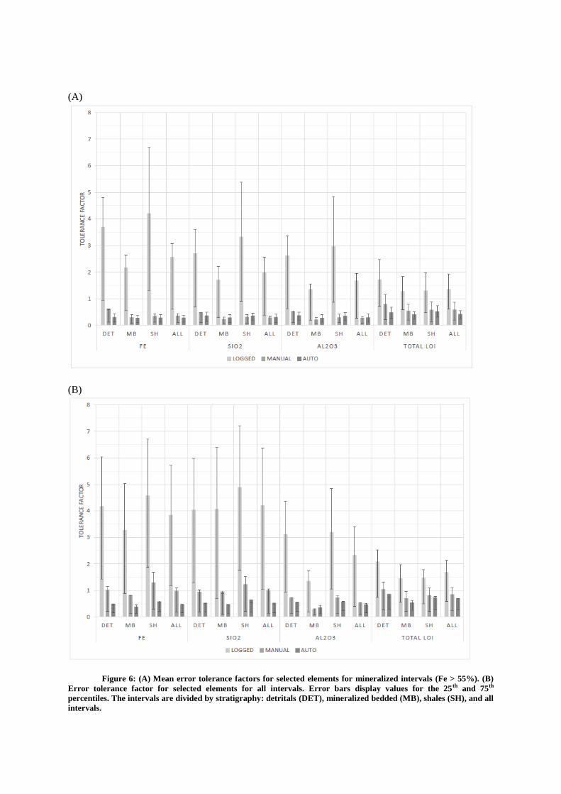
(A)

(B)

Figure 6: (A) Mean error tolerance factors for selected elements for mineralized intervals (Fe > 55%). (B)

Error tolerance factor for selected elements for all intervals. Error bars display values for the 25th and 75th

percentiles. The intervals are divided by stratigraphy: detritals (DET), mineralized bedded (MB), shales (SH), and all

intervals.

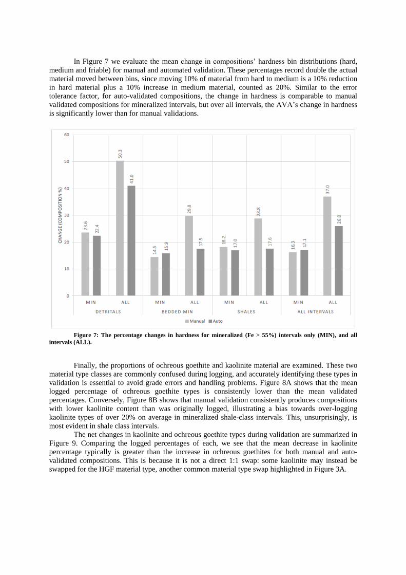
In Figure 7 we evaluate the mean change in compositions’ hardness bin distributions (hard,

medium and friable) for manual and automated validation. These percentages record double the actual

material moved between bins, since moving 10% of material from hard to medium is a 10% reduction

in hard material plus a 10% increase in medium material, counted as 20%. Similar to the error

tolerance factor, for auto-validated compositions, the change in hardness is comparable to manual

validated compositions for mineralized intervals, but over all intervals, the AVA’s change in hardness

is significantly lower than for manual validations.

Figure 7: The percentage changes in hardness for mineralized (Fe > 55%) intervals only (MIN), and all

intervals (ALL).

Finally, the proportions of ochreous goethite and kaolinite material are examined. These two

material type classes are commonly confused during logging, and accurately identifying these types in

validation is essential to avoid grade errors and handling problems. Figure 8A shows that the mean

logged percentage of ochreous goethite types is consistently lower than the mean validated

percentages. Conversely, Figure 8B shows that manual validation consistently produces compositions

with lower kaolinite content than was originally logged, illustrating a bias towards over-logging

kaolinite types of over 20% on average in mineralized shale-class intervals. This, unsurprisingly, is

most evident in shale class intervals.

The net changes in kaolinite and ochreous goethite types during validation are summarized in

Figure 9. Comparing the logged percentages of each, we see that the mean decrease in kaolinite

percentage typically is greater than the increase in ochreous goethites for both manual and auto-

validated compositions. This is because it is not a direct 1:1 swap: some kaolinite may instead be

swapped for the HGF material type, another common material type swap highlighted in Figure 3A.

(A)

(B)

Figure 8: (A) Ochreous goethite compositions for mineralized (MIN) and all intervals, broken down by

stratigraphy. (B) Kaolinite compositions for mineralized (MIN) and all intervals, broken down by stratigraphy.

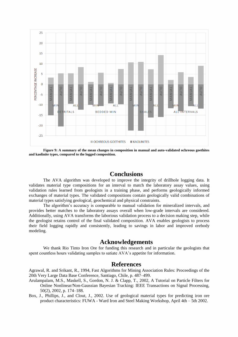
Figure 9: A summary of the mean changes in composition in manual and auto-validated ochreous goethites

and kaolinite types, compared to the logged composition.

Conclusions The AVA algorithm was developed to improve the integrity of drillhole logging data. It

validates material type compositions for an interval to match the laboratory assay values, using

validation rules learned from geologists in a training phase, and performs geologically informed

exchanges of material types. The validated compositions contain geologically valid combinations of

material types satisfying geological, geochemical and physical constraints.

The algorithm’s accuracy is comparable to manual validation for mineralized intervals, and

provides better matches to the laboratory assays overall when low-grade intervals are considered.

Additionally, using AVA transforms the laborious validation process to a decision making step, while

the geologist retains control of the final validated composition. AVA enables geologists to process

their field logging rapidly and consistently, leading to savings in labor and improved orebody

modeling.

Acknowledgements We thank Rio Tinto Iron Ore for funding this research and in particular the geologists that

spent countless hours validating samples to satiate AVA’s appetite for information.

References Agrawal, R. and Srikant, R., 1994, Fast Algorithms for Mining Association Rules: Proceedings of the

20th Very Large Data Base Conference, Santiago, Chile, p. 487–499.

Arulampalam, M.S., Maskell, S., Gordon, N. J. & Clapp, T., 2002, A Tutorial on Particle Filters for

Online Nonlinear/Non-Gaussian Bayesian Tracking: IEEE Transactions on Signal Processing,

50(2), 2002, p. 174–188.

Box, J., Phillips, J., and Clout, J., 2002. Use of geological material types for predicting iron ore

product characteristics: FUWA - Ward Iron and Steel Making Workshop, April 4th – 5th 2002.

Morris R.C. 1994, Detrital Iron Deposits of the Hamersley Province: CSIRO Division of Exploration

and Mining GDSR 2536, 233p.

Paine, M.D., Boyle, C., Lewan, A., Phuak, E., Mackenzie, P., Ryan, E., 2016, Geometallurgy at RTIO

– a new angle on an old concept: Third AusIMM International Geometallurgy Conference, p.

55–61.

Sommerville, B., Boyle, C., Brajkovich, N., Savory, P. and A.-A. Latscha, A.-A., 2014, Mineral

resource estimation of the Brockman 4 iron ore deposit in the Pilbara region: Special Issue on

Mineral Resource Estimation, Applied Earth Science, p. 135–145.

Trendall, A. F. and Blockley, J. G., 1970, The iron formations of the Precambrian Hamersley Group,

Western Australia, with special reference to the associated crocidolite: Bulletin 119, Geological

Survey of Western Australia, 365p.