Embed Size (px)
Citation preview
A Coupled-Adjoint Method for Aerodynamic and
Aeroacoustic Optimization
Thomas D. Economon
⇤, Francisco Palacios
†, and Juan J. Alonso
‡,
Stanford University, Stanford, CA 94305, U.S.A.
Designing quieter, more e�cient aerospace systems will require coupled, high fidelity
analysis and optimization in the areas of aerodynamics and aeroacoustics. This paper
presents a methodology for addressing these two disciplines via separate numerical methods
coupled within a single design framework. After detailing the governing flow and time-
accurate adjoint equations for unsteady aerodynamics, a continuous adjoint formulation
for the control of noise is developed. In order to obtain the required remote sensitivity
information for an o↵-body observer of noise, the adjoint formulations for aerodynamics and
aeroacoustics are coupled through an adjoint boundary condition. The result is an e�cient,
adjoint-based methodology for design problems involving both aerodynamic performance
and noise control or other multidisciplinary applications featuring multiple solvers with
one-way coupling.
Nomenclature
V ariable Definition
a Speed of soundc Airfoil chord length~d Force projection vectorf Function describing the acoustic surface, f = 0jS
Scalar function defined at each point on S~n Unit normal vectorp Static pressurep1 Freestream pressurep0 Acoustic pressure, p0 = p � p1to
Initial timetf
Final time~u
b
Control volume boundary velocity~v Flow velocity vector in the intertial framev1 Freestream velocity~w Velocity of the acoustic surface~A Inviscid flux Jacobian matricesA
z
Projected area in the z-directionC
d
Coe�cient of dragC
l
Coe�cient of liftC
p
Coe�cient of pressureE Total energy per unit mass~F Euler convective fluxes~F
mov
Euler convective fluxes for moving control volumesH Stagnation enthalpy
⇤Ph.D. Candidate, Department of Aeronautics & Astronautics, AIAA Student Member.†Engineering Research Associate, Department of Aeronautics & Astronautics, AIAA Member.‡Associate Professor, Department of Aeronautics & Astronautics, AIAA Senior Member.
1 of 17
American Institute of Aeronautics and Astronautics
¯̄I Identity matrixI Objective function for the acoustic problemJ Objective function defined as an integral over SM1 Freestream Mach numberN (⇢0) Governing equation for acousticsP Compressive stress tensorP 0 Fluctuating components of the stress tensorQ Source term(s)R(U) System of governing flow equationsS Solid wall flow domain boundary (design surface)T Time interval, t
f
� to
U Vector of conservative variablesW Vector of characteristic variables↵ Angle of attack� Sideslip angle� Ratio of specific heats, � = 1.4 for air⇢ Fluid density⇢1 Freestream density⇢0 Acoustic density, ⇢0 = ⇢� ⇢1� Acoustic adjoint variable~' Flow adjoint velocity vector! Angular frequency!
r
Reduced frequency, !c
2v1� Domain boundary Vector of flow adjoint variables⌦ Problem domain
Mathematical Notation
~b Spatial vector b 2 Rn, where n is the dimension of the physical cartesian space (in general, 2 or 3)B Column vector or matrix B, unless capitalized symbol clearly defined otherwise~B ~B = (B
x
, By
) in two dimensions or ~B = (Bx
, By
, Bz
) in three dimensionsr(·) Gradient operatorr · (·) Divergence operatorr2(·) Laplacian operator@
n
(·) Normal gradient operator at a surface point, ~nS
·r(·)r
S
(·) Tangential gradient operator at a surface point, r(·) � @n
(·)· Vector inner product⇥ Vector cross product⌦ Vector outer productBT Transpose operation on column vector or matrix B�(·) Denotes first variation of a quantity, unless otherwise specified as the Dirac delta function
I. Introduction and Motivation
Environmental pressures to decrease fuel burn, emissions, and noise continue to drive the need forquieter, more e�cient aircraft and aircraft propulsion technology. These environmental challenges also
o↵er an opportunity for the aircraft designer to take advantage of synergistic interactions between componentsof the configuration design. One example of this interaction e↵ect involves the installation of next generationpropulsion systems, such as the open rotor engine, which may be more e�cient at the cost of increasednoise. New proposals for unconventional aircraft configurations or engine placement may target enhancedaerodynamic performance, noise shielding, or provide safety in the event of blade-out. These complex systemswill require multidisciplinary, high fidelity analysis and system-level integration studies in order to assesstheir viability. Other challenges might include reducing airframe or jet noise without incurring performancepenalties for a particular vehicle.
The development of a revolutionary technology comes hand in hand with the issue of how to optimize
2 of 17
American Institute of Aeronautics and Astronautics
and integrate it into aerospace systems. Successful deployment of new technology will require novel multidis-ciplinary design, analysis, and optimization (MDAO) approaches for complex aerospace systems which arerooted in physics-based predictions. As mentioned, two disciplines of particular interest are aerodynamics andaeroacoustics. High-fidelity analysis and design tools will be needed to understand the interaction betweenthese disciplines and to aid the designer in extracting the best performance with minimal noise penalties.Optimal shape design and aeroacoustic analysis via computational fluid dynamics (CFD) and computationalaeroacoustics (CAA), respectively, are two candidate toolsets for this type of multidisciplinary research.While it is possible to directly compute acoustic behavior through CFD alone, these two disciplines are oftenconsidered separately, as they will be in this article, for computational e�ciency, accuracy, or flexibilityreasons.
In the context of optimal shape design, adjoint-based formulations have a rich history in aeronautics,and their e↵ectiveness for the design of aircraft configurations in cruise and other steady problems is wellestablished.1,2, 3 Less common and more di�cult are adjoint formulations for unsteady aerodynamic problemsin part due to prohibitive data storage requirements. Recent work has demonstrated the viability of unsteadyadjoint approaches for airfoil applications5 and turbulent flows on dynamic meshes.6
⌦�1
S~n
S
~n�1
Figure 1. Notional schematic of the flow do-main, ⌦, and the disconnected boundaries withtheir corresponding surface normals, S and�1.
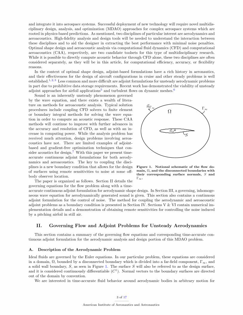
Sound is an inherently unsteady phenomenon governedby the wave equation, and there exists a wealth of litera-ture on methods for aeroacoustic analysis. Typical solutionprocedures include coupling CFD solvers to finite elementor boundary integral methods for solving the wave equa-tion in order to compute an acoustic response. These CAAmethods will continue to improve with further advances inthe accuracy and resolution of CFD, as well as with an in-crease in computing power. While the analysis problem hasreceived much attention, design problems involving aeroa-coustics have not. There are limited examples of adjoint-based and gradient-free optimization techniques that con-sider acoustics for design.7 With this paper we present time-accurate continuous adjoint formulations for both aerody-namics and aeroacoustics. The key to coupling the disci-plines is a new boundary condition that allows for the designof surfaces using remote sensitivities to noise at some o↵-body observer location.
The paper is organized as follows. Section II details thegoverning equations for the flow problem along with a time-accurate continuous adjoint formulation for aerodynamic shape design. In Section III, a governing, inhomoge-neous wave equation for aerodynamically generated sound is given. This section also contains a continuousadjoint formulation for the control of noise. The method for coupling the aerodynamic and aeroacousticadjoint problems as a boundary condition is presented in Section IV. Sections V & VI contain numerical im-plementation details and a demonstration of obtaining remote sensitivities for controlling the noise inducedby a pitching airfoil in still air.
II. Governing Flow and Adjoint Problems for Unsteady Aerodynamics
This section contains a summary of the governing flow equations and corresponding time-accurate con-tinuous adjoint formulation for the aerodynamic analysis and design portion of this MDAO problem.
A. Description of the Aerodynamic Problem
Ideal fluids are governed by the Euler equations. In our particular problem, these equations are consideredin a domain, ⌦, bounded by a disconnected boundary which is divided into a far-field component, �1, anda solid wall boundary, S, as seen in Figure 1. The surface S will also be referred to as the design surface,and it is considered continuously di↵erentiable (C1). Normal vectors to the boundary surfaces are directedout of the domain by convention.
We are interested in time-accurate fluid behavior around aerodynamic bodies in arbitrary motion for
3 of 17
American Institute of Aeronautics and Astronautics
situations where viscous e↵ects can be considered negligible. The governing flow equations in the limit ofvanishing viscosity are the compressible Euler equations which can be expressed in conservation form as
8
>
<
>
:
@U
@t
+ r · ~Fmov
= 0 in ⌦,
(~v � ~ub
) · ~nS
= 0 on S,
W+�1
(U) = W1 on �1,
(1)
where
U =
8
>
<
>
:
⇢
⇢~v
⇢E
9
>
=
>
;
, ~Fmov
=
8
>
<
>
:
⇢(~v � ~ub
)
⇢~v ⌦ (~v � ~ub
) + ¯̄Ip
⇢E(~v � ~ub
) + p~v
9
>
=
>
;
, (2)
⇢ is the fluid density, ~v = {u, v, w}T is the flow velocity, ~ub
is the boundary velocity for a control volumein motion, E is the total energy per unit mass, and p is the static pressure. The second line of Equation 1represents the flow tangency condition at a solid wall. The final line represents a characteristic-basedboundary condition at the far-field where, in general, the fluid states at the boundaries are updated dependingon the sign of the eigenvalues. The boundary conditions take into account any boundary velocity due tocontrol volume motion. In order to close the system of equations after assuming a perfect gas, the pressureis determined from
p = (� � 1)⇢
E � 1
2(~v · ~v)
�
, (3)
and the stagnation enthalpy is given by
H = E +p
⇢. (4)
B. Surface Sensitivities via a Time-Accurate Continuous Adjoint Approach
The objective of this section is to describe the way in which we quantify the influence of geometric modifi-cations on the pressure distribution at a solid surface in the flow domain.
A typical shape optimization problem seeks the minimization of a certain cost function, J , with respectto changes in the shape of the boundary, S. Therefore, we will concentrate on functionals defined as time-averaged integrated quantities on the solid surface S,
J =1
T
Z
t
f
t
o
Z
S
jS
ds dt, (5)
where jS
is a time-dependent scalar function defined at each point on S.
�S~nS
S
S0
~x
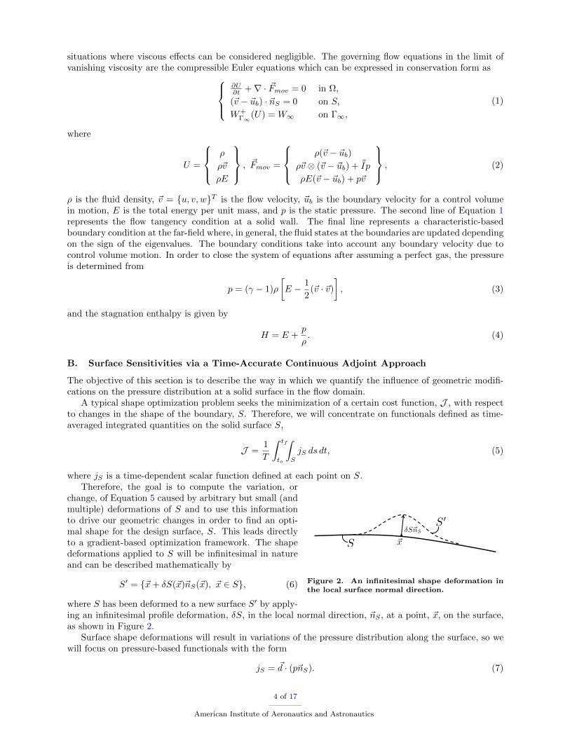
Figure 2. An infinitesimal shape deformation inthe local surface normal direction.
Therefore, the goal is to compute the variation, orchange, of Equation 5 caused by arbitrary but small (andmultiple) deformations of S and to use this informationto drive our geometric changes in order to find an opti-mal shape for the design surface, S. This leads directlyto a gradient-based optimization framework. The shapedeformations applied to S will be infinitesimal in natureand can be described mathematically by
S0 = {~x + �S(~x)~nS
(~x), ~x 2 S}, (6)
where S has been deformed to a new surface S0 by apply-ing an infinitesimal profile deformation, �S, in the local normal direction, ~n
S
, at a point, ~x, on the surface,as shown in Figure 2.
Surface shape deformations will result in variations of the pressure distribution along the surface, so wewill focus on pressure-based functionals with the form
jS
= ~d · (p~nS
). (7)
4 of 17
American Institute of Aeronautics and Astronautics
The vector ~d is the force projection vector, and it is an arbitrary, constant vector which can be chosen torelate the pressure, p, at the surface to a desired quantity of interest. For aerodynamic applications, likelycandidates are
~d =
8
>
>
>
>
>
>
<
>
>
>
>
>
>
:
⇣
1C1
⌘
(cos ↵ cos �, sin ↵ cos �, sin �), CD
Drag coe�cient,⇣
1C1
⌘
(� sin ↵, cos ↵, 0), CL
Lift coe�cient,⇣
1C1
⌘
(� sin � cos ↵,� sin � sin ↵, cos �), CSF
Side-force coe�cient,⇣
1C1C
D
⌘
(� sin↵� C
L
C
D
cos↵ cos�,�C
L
C
D
sin�, cos↵� C
L
C
D
sin↵ cos�), C
L
C
D
L/D,
(8)where C1 = 1
2v21⇢1A
z
, v1 is the freestream velocity, ⇢1 is the freestream density, and Az
is the referencearea. In practice for a three-dimensional surface, we often sum up all positive components of the normalsurface vectors in the z-direction in order to calculate the projection A
z
. A pre-specified reference area canalso be used in a similar fashion, and this is an established procedure in applied aerodynamics.
The minimization of Eqn. 5 can be considered a problem of optimal control whereby the behavior of thegoverning flow equation system is controlled by the surface shape with deformations of the surface actingas the control input. Furthermore, any variations of the flow variables due to surface deformations areconstrained to satisfy the system of governing flow equations,
R(U) =@U
@t+ r · ~F
mov
=@U
@t+ r · ~F �r · (U ⌦ ~u
b
) = 0, (9)
where the terms involving the control volume motion have been separated from the traditional Euler fluxes.Mathematically, the constrained optimization problem can be formulated as follows:
Minimize J = 1T
R
t
f
t
o
R
S
~d · (p~nS
) ds dt
such that R(U) = 0(10)
Following the adjoint approach to optimal design, the constrained optimization problem in Equation 10 canbe transformed into an unconstrained optimization problem by adding the inner product of an unsteadyadjoint variable vector, , and the governing equations integrated over the domain (space and time) to formthe Lagrangian:
J =1
T
Z
t
f
t
o
Z
S
~d · (p~nS
) ds dt +1
T
Z
t
f
t
o
Z
⌦ TR(U) d⌦ dt, (11)
where we have introduced the adjoint variables, which operate as Lagrange multipliers and are defined as
=
8
>
>
>
>
>
<
>
>
>
>
>
:
⇢
⇢u
⇢v
⇢w
⇢E
9
>
>
>
>
>
=
>
>
>
>
>
;
=
8
>
<
>
:
⇢
~'
⇢E
9
>
=
>
;
. (12)
To find the gradient information needed to minimize the objective function, we take the first variation ofEqn. 11 with respect to perturbations of the surface shape:
�J =1
T
Z
t
f
t
o
Z
S
(~d ·rp)�S ds dt +1
T
Z
t
f
t
o
Z
S
(~d · ~nS
)�p ds dt +1
T
Z
t
f
t
o
Z
⌦ T �R(U) d⌦ dt. (13)
It is important to note that the first two terms of Eqn. 13 are found by using a result from previous workby the second author8 based on di↵erential geometry formulas, and this is a key feature di↵erentiating thecurrent formulation from other adjoint approaches. The third term of Equation 13 can be expanded byincluding the linearized version of the governing equations with respect to small perturbations of the design
5 of 17
American Institute of Aeronautics and Astronautics
surface,
�R(U) =@
@t(�U) + r · � ~F �r · �(U ⌦ ~u
b
)
=@
@t(�U) + r ·
@ ~F
@U�U
!
�r ·
@(U ⌦ ~ub
)
@U�U
�
=@
@t(�U) + r ·
⇣
~A � ¯̄I~ub
⌘
�U, (14)
along with the linearized form of the boundary condition at the surface,
�~v · ~nS
= �(~v � ~ub
) · �~nS
� @n
(~v � ~ub
) · ~nS
�S, (15)
where ~A is the Jacobian of ~F using conservative variables. Equation 14 can now be introduced into Equa-tion 13 to produce
�J =1
T
Z
t
f
t
o
Z
S
(~d ·rp)�S ds dt +1
T
Z
t
f
t
o
Z
S
(~d · ~nS
)�p ds dt +1
T
Z
t
f
t
o
Z
⌦ T
@
@t(�U) d⌦ dt
+1
T
Z
t
f
t
o
Z
⌦ Tr ·
⇣
~A � ¯̄I~ub
⌘
�U d⌦ dt. (16)
By removing any dependence on variations of the flow variables, �p, the variation of the objective functionfor multiple surface deformations can be found without the need for multiple flow solutions which results in acomputationally e�cient method for aerodynamic design involving many design variables. We now performmanipulations to remove this dependence. After changing the order of integration, integrating the thirdterm of Eqn. 16 by parts gives
Z
⌦
Z
t
f
t
o
T
@
@t(�U) d⌦ dt =
Z
⌦
⇥
T �U⇤
t
f
t
o
d⌦�Z
⌦
Z
t
f
t
o
@ T
@t�U d⌦ dt. (17)
A zero-value initial condition for the adjoint variables can be imposed, and assuming an unsteady flow withperiodic behavior, the first term on the right hand side of Eqn. 17 can be eliminated with the followingtemporal conditions (the cost function does not depend on t
f
):
(~x, to
) = 0, (18)
(~x, tf
) = 0. (19)
Now, integrating the fourth term of Eqn. 16 yields
Z
t
f
t
o
Z
⌦ Tr ·
⇣
~A � ¯̄I~ub
⌘
�U d⌦ dt =
Z
t
f
t
o
Z
⌦r ·h
T
⇣
~A � ¯̄I~ub
⌘
�Ui
d⌦ dt �Z
t
f
t
o
Z
⌦r T ·
⇣
~A � ¯̄I~ub
⌘
�Ud⌦ dt,
(20)
and applying the divergence theorem to the first term on the right hand side of Eqn. 20, assuming a smoothsolution, gives
Z
t
f
t
o
Z
⌦ Tr ·
⇣
~A � ¯̄I~ub
⌘
�U d⌦ dt =
Z
t
f
t
o
Z
S
T
⇣
~A � ¯̄I~ur
⌘
· ~nS
�Uds dt
+
Z
t
f
t
o
Z
�1
T
⇣
~A � ¯̄I~ur
⌘
· ~nS
�Uds dt
�Z
t
f
t
o
Z
⌦r T ·
⇣
~A � ¯̄I~ub
⌘
�Ud⌦ dt. (21)
With the appropriate choice of characteristic-based boundary conditions, the integral over the far-field bound-ary can be forced to vanish. Combining and rearranging the results from Eqns. 16, 17, 18, 19 & 21 yields
6 of 17
American Institute of Aeronautics and Astronautics
an intermediate expression for the variation of the cost function,
�J =1
T
Z
t
f
t
o
Z
S
(~d ·rp)�S ds dt +1
T
Z
t
f
t
o
Z
S
(~d · ~nS
)�p ds dt +
Z
t
f
t
o
Z
S
T
⇣
~A � ¯̄I~ub
⌘
· ~nS
�Uds
� 1
T
Z
t
f
t
o
Z
⌦
@ T
@t+ r T ·
⇣
~A � ¯̄I~ub
⌘
�
�U d⌦ dt. (22)
The final term of Eqn. 22 can also be made to vanish, if its integrand is zero at every point in the domain.When set equal to zero, the terms within the brackets constitute the set of partial di↵erential equations whichare commonly referred to as the adjoint equations. Therefore, the domain integral will vanish provided thatthe adjoint equations are satisfied as
@ T
@t+ r T ·
⇣
~A � ¯̄I~ub
⌘
= 0 in ⌦, (23)
or after taking the transpose
@
@t+⇣
~A � ¯̄I~ub
⌘
T
·r = 0 in ⌦. (24)
The accompanying boundary condition will be given below. Furthermore, the surface integral in the thirdterm on the right hand side of Eqn. 22 can be evaluated given our knowledge of ~A, ~u
b
, the wall boundarycondition, (~v � ~u
b
) · ~nS
= 0, and the linearized wall boundary condition in Eqn. 15. By leveraging previousderivation by the authors9 with some slight modifications and including time integration, it can be shownthat evaluating the surface integral and rearranging the variation of the functional gives
�J =1
T
Z
t
f
t
o
Z
S
h
~d ·rp + (r · ~v)#+ (~v � ~ub
) ·r(#)i
�S ds dt +1
T
Z
t
f
t
o
Z
S
h
~d · ~nS
� ~nS
· ~'� ⇢E
(~v · ~nS
)i
�p ds dt,
(25)
where # = ⇢ ⇢
+ ⇢~v · ~' + ⇢H ⇢E
. Therefore, the adjoint equations with the admissible adjoint boundarycondition that eliminates the dependence on the fluid flow variations (�p) by forcing the second term on theright hand side of Eqn. 25 to vanish can be written as
8
<
:
@ @t
+⇣
~A � ¯̄I~ub
⌘
T
·r = 0 in ⌦,
~nS
· ~' = ~d · ~nS
� ⇢E
(~v · ~nS
) on S,(26)
and the variation of the objective function becomes
�J =1
T
Z
t
f
t
o
Z
S
h
~d ·rp + (r · ~v)#+ (~v � ~ub
) ·r(#)i
�S ds dt =1
T
Z
t
f
t
o
Z
S
@J@S
�S ds, (27)
where @J@S
= ~d ·rp + (r ·~v)#+ (~v � ~ub
) ·r(#) is what we call the surface sensitivity. The surface sensitivityprovides a measure of the variation of the objective function with respect to infinitesimal variations of thesurface shape in the direction of the local surface normal. This value is computed at each surface node of thenumerical grid at each physical time step with negligible computational cost. Note that the final expressionfor the variation involves only a surface integral at each physical time step and has no dependence on thevolume mesh.
III. Governing Wave and Adjoint Problems for Aeroacoustics
In this section we detail the prediction method for aerodynamically generated sound and also present anew continuous adjoint formulation for the control of noise.
A. Description of the Aeroacoustic Problem
We are interested in predicting and controlling the noise generated by aerodynamic surfaces that might bein motion, and for this aeroacoustic problem, perturbations in density, ⇢0 where ⇢0(~x, t) = ⇢(~x, t)� ⇢1, form
7 of 17
American Institute of Aeronautics and Astronautics
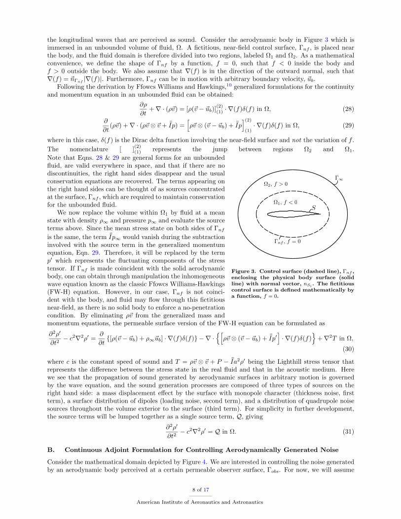
the longitudinal waves that are perceived as sound. Consider the aerodynamic body in Figure 3 which isimmersed in an unbounded volume of fluid, ⌦. A fictitious, near-field control surface, �
nf
, is placed nearthe body, and the fluid domain is therefore divided into two regions, labeled ⌦1 and ⌦2. As a mathematicalconvenience, we define the shape of �
nf
by a function, f = 0, such that f < 0 inside the body andf > 0 outside the body. We also assume that r(f) is in the direction of the outward normal, such thatr(f) = ~n�
nf
|r(f)|. Furthermore, �nf
can be in motion with arbitrary boundary velocity, ~ub
.Following the derivation by Ffowcs Williams and Hawkings,10 generalized formulations for the continuity
and momentum equation in an unbounded fluid can be obtained:
@⇢
@t+ r · (⇢~v) = [⇢(~v � ~u
b
)](2)(1) ·r(f)�(f) in ⌦, (28)
@
@t(⇢~v) + r · (⇢~v ⌦ ~v + ¯̄Ip) =
h
⇢~v ⌦ (~v � ~ub
) + ¯̄Ipi(2)
(1)·r(f)�(f) in ⌦, (29)
where in this case, �(f) is the Dirac delta function involving the near-field surface and not the variation of f .
The nomenclature [ ](2)(1) represents the jump between regions ⌦2 and ⌦1.
�1
S
�nf
, f = 0
⌦1, f < 0
⌦2, f > 0
Figure 3. Control surface (dashed line), �nf
,enclosing the physical body surface (solidline) with normal vector, n
S
i
. The fictitiouscontrol surface is defined mathematically bya function, f = 0.
Note that Eqns. 28 & 29 are general forms for an unboundedfluid, are valid everywhere in space, and that if there are nodiscontinuities, the right hand sides disappear and the usualconservation equations are recovered. The terms appearing onthe right hand sides can be thought of as sources concentratedat the surface, �
nf
, which are required to maintain conservationfor the unbounded fluid.
We now replace the volume within ⌦1 by fluid at a meanstate with density ⇢1 and pressure p1 and evaluate the sourceterms above. Since the mean stress state on both sides of �
nf
is the same, the term ¯̄Ip1 would vanish during the subtractioninvolved with the source term in the generalized momentumequation, Eqn. 29. Therefore, it will be replaced by the termp0 which represents the fluctuating components of the stresstensor. If �
nf
is made coincident with the solid aerodynamicbody, one can obtain through manipulation the inhomogeneouswave equation known as the classic Ffowcs Williams-Hawkings(FW-H) equation. However, in our case, �
nf
is not coinci-dent with the body, and fluid may flow through this fictitiousnear-field, as there is no solid body to enforce a no-penetrationcondition. By eliminating ⇢~v from the generalized mass andmomentum equations, the permeable surface version of the FW-H equation can be formulated as
@2⇢0
@t2� c2r2⇢0 =
@
@t{[⇢(~v � ~u
b
) + ⇢1~ub
] ·r(f)�(f)}�r ·nh
⇢~v ⌦ (~v � ~ub
) + ¯̄Ip0i
·r(f)�(f)o
+ r2T in ⌦,
(30)
where c is the constant speed of sound and T = ⇢~v ⌦ ~v + P � ¯̄Ia2⇢0 being the Lighthill stress tensor thatrepresents the di↵erence between the stress state in the real fluid and that in the acoustic medium. Herewe see that the propagation of sound generated by aerodynamic surfaces in arbitrary motion is governedby the wave equation, and the sound generation processes are composed of three types of sources on theright hand side: a mass displacement e↵ect by the surface with monopole character (thickness noise, firstterm), a surface distribution of dipoles (loading noise, second term), and a distribution of quadrupole noisesources throughout the volume exterior to the surface (third term). For simplicity in further development,the source terms will be lumped together as a single source term, Q, giving
@2⇢0
@t2� c2r2⇢0 = Q in ⌦. (31)
B. Continuous Adjoint Formulation for Controlling Aerodynamically Generated Noise
Consider the mathematical domain depicted by Figure 4. We are interested in controlling the noise generatedby an aerodynamic body perceived at a certain permeable observer surface, �
obs
. For now, we will assume
8 of 17
American Institute of Aeronautics and Astronautics

that the aerodynamic body can be represented by a distribution of sources, Q, in the domain, ⌦, without de-tailing their formulation. In this manner, we can consider the general problem of controlling wave behavior re-sulting from an arbitrary distribution of sources, which might have wider applicability to problems in physicsand engineering.
�obs
⌦
Q(~x, t)
~n�obs
Figure 4. Schematic of the domain, ⌦, for theacoustic problem. We are concerned with thenoise generated by an arbitrary distribution ofsources, Q, observed at a permeable, surface,�obs
.
One approach for controlling noise is to minimize a measureof the total sound amplitude integrated over the observer sur-face. A suitable cost function for this problem involving theacoustic pressure, or the acoustic density (for linear acousticsp0 = c2⇢0), can be written as
I =1
T
Z
t
f
t
o
Z
�obs
p02 ds dt =1
T
Z
t
f
t
o
Z
�obs
(c2⇢0)2 ds dt. (32)
Other cost functions are possible, such as matching a speci-fied target acoustic signature in time on �
obs
. For instance,this target signature might call for a reduction in the totalstrength of the noise, or perhaps an adjustment in the fre-quency content. Controlling the noise requires knowledge ofthe system, and in our problem, the generation and propaga-tion of aerodynamically generated sound is governed by aninhomogeneous wave equation (FW-H equation):
N (⇢0) =@2⇢0
@t2� c2r2⇢0 �Q = 0, (33)
where ~x 2 ⌦, t 2 [to
, tf
], and Q is the distribution of sources.The sources will act as the input for controlling the noise
at the observer surface. In words, we are seeking to minimize the total noise at �obs
through changes inthe source terms, Q, that are propagated through the domain by the wave equation. Mathematically, theoptimization problem can be formulated as follows:
Minimize I = 1T
R
t
f
t
o
R
�obs
(c2⇢0)2 ds dt
such that N (⇢0) = 0(34)
Following the adjoint approach to optimal design, the constrained optimization problem in Equation 34can be transformed into an unconstrained optimization problem by taking the inner product of an adjointvariable, �, and the governing equation, N (⇢0), to form the Lagrangian:
I =1
T
Z
t
f
t
o
Z
�obs
(c2⇢0)2 ds dt +1
T
Z
t
f
t
o
Z
⌦� N (⇢0) d⌦ dt. (35)
The gradient information needed for minimizing I can be obtained by taking its first variation with respectto perturbations in the source term,
�I =1
T
Z
t
f
t
o
Z
�obs
2c2⇢0�⇢0 ds dt +1
T
Z
t
f
t
o
Z
⌦� �N (⇢0) d⌦ dt
=1
T
Z
t
f
t
o
Z
�obs
2c2⇢0�⇢0 ds dt +1
T
Z
t
f
t
o
Z
⌦�
@2
@t2(�⇢0) � c2r2(�⇢0) � �Q
�
d⌦ dt.
=1
T
Z
t
f
t
o
Z
�obs
2c2⇢0�⇢0 ds dt +1
T
Z
t
f
t
o
Z
⌦�@2
@t2(�⇢0) d⌦ dt � c2
T
Z
t
f
t
o
Z
⌦�r2(�⇢0) d⌦ dt � 1
T
Z
t
f
t
o
Z
⌦� �Q d⌦ dt.
(36)
After changing the order of integration, integrating the second term on the right hand side of Equation 36by parts gives
Z
⌦
Z
t
f
t
o
�@2
@t2(�⇢0) dt d⌦ =
Z
⌦
�@
@t(�⇢0)
�
t
f
t
o
d⌦�Z
⌦
Z
t
f
t
o
@�
@t
@
@t(�⇢0) dt d⌦, (37)
9 of 17
American Institute of Aeronautics and Astronautics

and again integrating the final term of Equation 37 by parts results inZ
⌦
Z
t
f
t
o
�@2
@t2(�⇢0) dt d⌦ =
Z
⌦
�@
@t(�⇢0)
�
t
f
t
o
d⌦�Z
⌦
@�
@t�⇢0�
t
f
t
o
d⌦+
Z
t
f
t
o
Z
⌦
@2�
@t2�⇢0 d⌦ dt, (38)
where the order of integration in the final term has been reversed again. Consider now the third term on theright hand side of Equation 36. Integrating by parts and using the divergence theorem (assuming a smoothsolution) yields
Z
t
f
t
o
Z
⌦�r2(�⇢0) d⌦ dt =
Z
t
f
t
o
Z
�obs
�r(�⇢0) · ~n�obs
ds dt �Z
t
f
t
o
Z
⌦r(�) ·r(�⇢0) d⌦ dt, (39)
and integrating the final term of Equation 39 by parts and using the divergence theorem a second timeresults inZ
t
f
t
o
Z
⌦�r2(�⇢0) d⌦ dt =
Z
t
f
t
o
Z
�obs
�r(�⇢0) · ~n�obs
ds dt �Z
t
f
t
o
Z
�obs
r(�) · ~n�obs
�⇢0 ds dt +
Z
t
f
t
o
Z
⌦r2� �⇢0 d⌦ dt.
(40)
The first term on the right hand side of Equation 40 can be eliminated by adding and subtracting again thesecond term, orZ
t
f
t
o
Z
⌦�r2(�⇢0) d⌦ dt
=
Z
t
f
t
o
Z
�obs
[�r(�⇢0) + r(�)�⇢0] · ~n�obs
ds dt � 2
Z
t
f
t
o
Z
�obs
r(�) · ~n�obs
�⇢0 ds dt +
Z
t
f
t
o
Z
⌦r2� �⇢0 d⌦ dt
=
Z
t
f
t
o
Z
�obs
r(� �⇢0) · ~n�obs
ds dt � 2
Z
t
f
t
o
Z
�obs
r(�) · ~n�obs
�⇢0 ds dt +
Z
t
f
t
o
Z
⌦r2� �⇢0 d⌦ dt
= �2
Z
t
f
t
o
Z
�obs
r(�) · ~n�obs
�⇢0 ds dt +
Z
t
f
t
o
Z
⌦r2� �⇢0 d⌦ dt, (41)
where we have used the mathematical identity that a gradient dotted with the normal and integrated overa closed surface is zero in going from the second to the third line.
After substituting the results from Eqns. 38 & 41 into Eqn. 36 and rearranging terms based on integraltype, the variation of the cost function becomes
�I =1
T
Z
t
f
t
o
Z
�obs
⇥
2c2⇢0 + 2c2r(�) · ~n�obs
⇤
�⇢0 ds dt +1
T
Z
⌦
�@
@t(�⇢0)
�
t
f
t
o
d⌦� 1
T
Z
⌦
@�
@t�⇢0�
t
f
t
o
d⌦
+1
T
Z
t
f
t
o
Z
⌦
@2�
@t2� c2r2�
�
�⇢0 d⌦ dt � 1
T
Z
t
f
t
o
Z
⌦� �Q d⌦ dt. (42)
Many of the terms in Eqn. 42 can be eliminated by satisfying the adjoint wave equation with the permissibleboundary and temporal conditions,
8
>
<
>
:
@
2�
@t
2 � c2r2� = 0 in ⌦, t 2 [to
, tf
],
@n
� = �⇢0, on �obs
, t 2 [to
, tf
]
�(~x, to
) = 0, @�(~x,t
o
)@t
= 0, in ⌦.
(43)
Note that the wave equation is self-adjoint, meaning that the corresponding adjoint equation is again thewave equation. As with the adjoint flow equations, if there is periodic behavior (the cost function does notdepend on t
f
), then the second and third integrals on the right hand side can be completely eliminated by
imposing �(~x, tf
) = 0 and @�(~x,t
f
)@t
= 0. The final result is a simple expression for the variation of the costfunction,
�I = � 1
T
Z
t
f
t
o
Z
⌦� �Q d⌦ dt. (44)
While the result in Eqn. 44 is general, we will limit the design space to a particular form for the sources,Q. More specifically, the sources will have the form of those appearing in the FW-H equation, or Q =Q(U(~x, t))�(f).
10 of 17
American Institute of Aeronautics and Astronautics
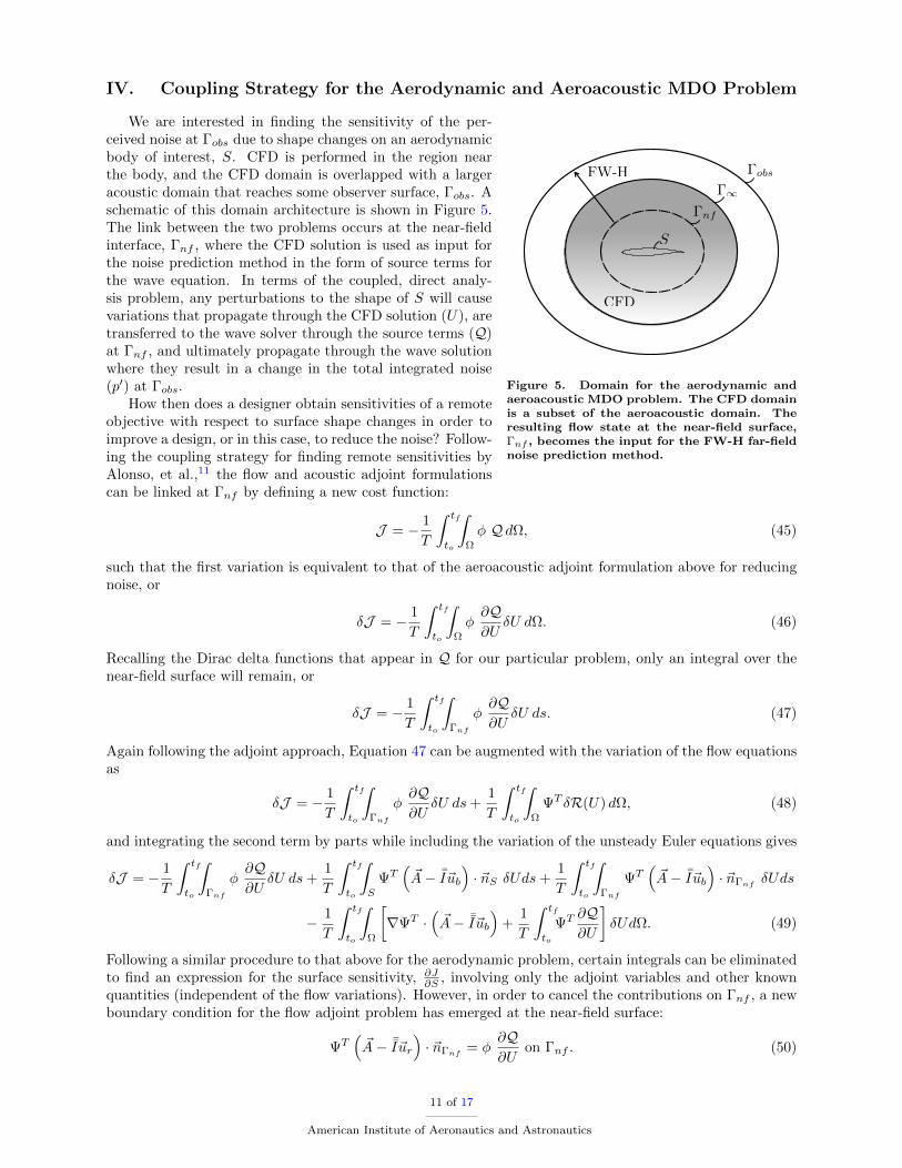
IV. Coupling Strategy for the Aerodynamic and Aeroacoustic MDO Problem
S
�obs
�nf
�1
CFD
FW-H
Figure 5. Domain for the aerodynamic andaeroacoustic MDO problem. The CFD domainis a subset of the aeroacoustic domain. Theresulting flow state at the near-field surface,�nf
, becomes the input for the FW-H far-fieldnoise prediction method.
We are interested in finding the sensitivity of the per-ceived noise at �
obs
due to shape changes on an aerodynamicbody of interest, S. CFD is performed in the region nearthe body, and the CFD domain is overlapped with a largeracoustic domain that reaches some observer surface, �
obs
. Aschematic of this domain architecture is shown in Figure 5.The link between the two problems occurs at the near-fieldinterface, �
nf
, where the CFD solution is used as input forthe noise prediction method in the form of source terms forthe wave equation. In terms of the coupled, direct analy-sis problem, any perturbations to the shape of S will causevariations that propagate through the CFD solution (U), aretransferred to the wave solver through the source terms (Q)at �
nf
, and ultimately propagate through the wave solutionwhere they result in a change in the total integrated noise(p0) at �
obs
.How then does a designer obtain sensitivities of a remote
objective with respect to surface shape changes in order toimprove a design, or in this case, to reduce the noise? Follow-ing the coupling strategy for finding remote sensitivities byAlonso, et al.,11 the flow and acoustic adjoint formulationscan be linked at �
nf
by defining a new cost function:
J = � 1
T
Z
t
f
t
o
Z
⌦� Q d⌦, (45)
such that the first variation is equivalent to that of the aeroacoustic adjoint formulation above for reducingnoise, or
�J = � 1
T
Z
t
f
t
o
Z
⌦�@Q@U
�U d⌦. (46)
Recalling the Dirac delta functions that appear in Q for our particular problem, only an integral over thenear-field surface will remain, or
�J = � 1
T
Z
t
f
t
o
Z
�nf
�@Q@U
�U ds. (47)
Again following the adjoint approach, Equation 47 can be augmented with the variation of the flow equationsas
�J = � 1
T
Z
t
f
t
o
Z
�nf
�@Q@U
�U ds +1
T
Z
t
f
t
o
Z
⌦ T �R(U) d⌦, (48)
and integrating the second term by parts while including the variation of the unsteady Euler equations gives
�J = � 1
T
Z
t
f
t
o
Z
�nf
�@Q@U
�U ds +1
T
Z
t
f
t
o
Z
S
T
⇣
~A � ¯̄I~ub
⌘
· ~nS
�Uds +1
T
Z
t
f
t
o
Z
�nf
T
⇣
~A � ¯̄I~ub
⌘
· ~n�nf
�Uds
� 1
T
Z
t
f
t
o
Z
⌦
r T ·⇣
~A � ¯̄I~ub
⌘
+1
T
Z
t
f
t
o
T
@Q@U
�
�Ud⌦. (49)
Following a similar procedure to that above for the aerodynamic problem, certain integrals can be eliminatedto find an expression for the surface sensitivity, @J
@S
, involving only the adjoint variables and other knownquantities (independent of the flow variations). However, in order to cancel the contributions on �
nf
, a newboundary condition for the flow adjoint problem has emerged at the near-field surface:
T
⇣
~A � ¯̄I~ur
⌘
· ~n�nf
= �@Q@U
on �nf
. (50)
11 of 17
American Institute of Aeronautics and Astronautics
By construction, the value here for �J is equivalent to the variation of the aeroacoustic cost function above,�I, so this new boundary condition represents the coupling of the two adjoint problems. The acoustic adjointsolution, �, will now be required on �
nf
at each time instance when solving the flow adjoint. Another keydi↵erence between the flow adjoint derivation above the coupled formulation described here is that there isno longer a dependence on the force projection vector, ~d. This is due to the choice of functional, as we areno longer interested in the pressure on the design surface. Instead, ~d = ~0, and the flow adjoint problembecomes,
8
<
:
@ @t
+⇣
~A � ¯̄I~ub
⌘
T
·r = 0 in ⌦,
~nS
· ~' = � ⇢E
(~v · ~nS
) on S,(51)
and the variation of the objective function becomes
�J =1
T
Z
t
f
t
o
Z
S
[(r · ~v)#+ (~v � ~ub
) ·r(#)] �S ds dt =1
T
Z
t
f
t
o
Z
S
@J@S
�S ds, (52)
V. Numerical Implementation
A. Numerical discretization of the Euler equations using FVM
Solution procedures for both the compressible Euler equations and the corresponding adjoint equations wereimplemented within the SU2 software suite (Stanford University Unstructured). This collection of C++codes is built specifically for PDE analysis and PDE-constrained optimization on unstructured meshes,and it is particularly well-suited for aerodynamic shape design. Modules for performing direct and adjointflow solutions, acquiring gradient information by projecting surface sensitivities into the design space, anddeforming meshes are included in the suite, amongst others. Scripts written in the Python programminglanguage are also used to automate execution of the SU2 suite components, especially for performing shapeoptimizations.
Both the direct and adjoint problems are solved using a Finite Volume Method (FVM) formulation withan edge-based structure. The solver is capable of both first and second order accurate dual-time steppingapproaches for time integration.12 The code is fully parallel and takes advantage of an agglomerationmultigrid approach for convergence acceleration. The unsteady Euler equations are spatially discretized usinga central scheme with JST-type artificial dissipation,13 and the adjoint equations use a slightly modified JSTscheme.
B. Numerical discretization of the wave equation using FEM
In this section a basic introduction to the Finite Element Method (FEM) technique is presented which hasalso been implemented within the SU2 software suite. The final objective is the numerical discretization ofthe wave equation with a source term Q = Q(~x).
@2V
@t2� c2~r2V = Q, in ⌦, t > 0 (53)
using Dirichlet and Neumann boundary conditions.Finite-element methods of solution are based upon approximations to a variational formulation of the
problem. A variational formulation requires the introduction of a space of trial functions, T = {V (t, ~x)},and a space of weighting functions W = {W (t, ~x)}. The problem consists in finding V (t, ~x) in T , satisfyingthe problem boundary conditions, such that
Z
⌦WT
✓
@2V
@t2� c2~r2V � Q
◆
d⌦ = 0 (54)
To produce an approximate solution to the variational problem, a grid of finite elements is constructedon the domain ⌦. It will be assumed that the discretization employs p nodes. Finite-dimensional subspaces
12 of 17
American Institute of Aeronautics and Astronautics

T (p) and W(p) of the trial and weighting function spaces, respectively, are defined by
T (p) =
(
V (p)(t, ~x) |V (p) =p
X
J=1
VJ
(t)NJ
(~x)
)
, (55)
W(p) =
(
W (p)(t, ~x) |W (p) =p
X
J=1
aJ
(t)NJ
(~x)
)
, (56)
where VJ
(t) is the value of V (p) at node J and time t. On the other hand, a1, a2, . . . , ap
are constant,and N
J
(~x) is the piecewise linear trial function associated with node J . We now apply the finite elementapproximation by discretizing the domain of the problem into elements and introducing functions whichinterpolate the solution over nodes that compose the elements. The Galerkin approximation is determinedby applying the variational formulation of (54) in the form: find V (p) in T (p), satisfying the problem boundaryconditions, such that
Z
⌦NT
I
✓
@2V
@t2� c2~r2V
◆
d⌦ =
Z
⌦NT
I
Q d⌦, (57)
for I = 1, 2, ..., p. The form assumed for V (p) in eq. (55) can now be inserted into the left hand side of (57)and the result writes as
Z
⌦NT
I
p
X
J=1
@2VJ
@t2N
J
� c2p
X
J=1
VJ
~r2NJ
!
d⌦ =
Z
⌦NT
I
Q d⌦, (58)
rearranging terms we obtain,
p
X
J=1
@2VJ
@t2
✓
Z
⌦NT
I
NJ
d⌦
◆
�p
X
J=1
c2VJ
✓
Z
⌦NT
I
~r2NJ
d⌦
◆
=
Z
⌦NT
I
Q d⌦, (59)
applying the Gauss’s divergence theorem
p
X
J=1
@2VJ
@t2
✓
Z
⌦NT
I
NJ
d⌦
◆
�p
X
J=1
c2VJ
✓
Z
�NT
I
⇣
~rNJ
· ~⌫⌘
d��Z
⌦
~rNT
I
· ~rNJ
d⌦
◆
=
Z
⌦NT
I
Q d⌦, (60)
where the boundary integral disappear unless we are computing an boundary element with non-homogeneousNeumann conditions (I is an exterior node). Finally, the result at a typical interior node I is
X
E2I
X
J2E
@2VJ
@t2
✓
Z
⌦E
NT
I
NJ
d⌦
◆
+X
E2I
X
J2E
c2VJ
✓
Z
⌦E
~rNT
I
· ~rNJ
d⌦
◆
=X
E2I
X
J2E
QJ
✓
Z
⌦E
NT
I
NJ
d⌦
◆
,
(61)where the first summation extend over the elements E in the numerical grid which contain node I and thesecond summation extends over nodes J of the elements E. ⌦
E
is the portion of ⌦ which is representedby element E. Note that the field variables Q are interpolated from the nodal variables by using the shapefunctions.
Finally the time discretization is performed using a a second order formula
@2W
@t2=
2un+1 � 5un�1 + 4un�1 � un�2
�t2(62)
or splitting the original equation into two partial di↵erential equations where only a first order time derivativeappears:
@W
@t= AW + g where, W =
"
V
U
#
, A =
"
0 I
c2~r2 0
#
, g =
"
0
Q
#
. (63)
13 of 17
American Institute of Aeronautics and Astronautics

C. Design Variable Definition and Mesh Deformation
The time-accurate continuous adjoint derivation presents a method for computing the variation of an ob-jective function with respect to infinitesimal surface shape deformations in the direction of the local surfacenormal at points on the design surface. While it is possible to use each surface node in the computationalmesh as a design variable capable of deformation, this approach is not often pursued in practice. A morepractical choice is to compute the surface sensitivities at each mesh node on the design surface and then toproject this information into a design space made up of a smaller set (possibly a complete basis) of designvariables. This procedure for computing the surface sensitivities can be used repeatedly in a gradient-basedoptimization framework in order to march the design surface shape toward an optimum through gradientprojection and mesh deformation.
In the two-dimensional airfoil calculations that follow, Hicks-Henne bump functions were employed14
which can be added to the original airfoil geometry to modify the shape. The Hicks-Henne function withmaximum at point x
n
is given by
fn
(x) = sin3(⇡xe
n), en
=log(0.5)
log(xn
), x 2 [0, 1], (64)
so that the total deformation of the surface can be computed as �y =P
N
n=1 �nfn
(x), with N being thenumber of bump functions and �
n
the design variable step. These functions are applied separately to theupper and lower surfaces. After applying the bump functions to recover a new surface shape with each designiteration, a spring analogy method is used to deform the volume mesh around the airfoil.15
VI. Demonstration of Remote Sensitivities for Noise Control
In order to demonstrate the coupled-adjoint method for use with design, a numerical experiment involvinga pitching NACA 64A010 airfoil was devised. Two overlapping grids were created for the CFD and CAAproblems, as shown in Figure 6. The meshes are identical, except within the �
nf
surface where the flowmesh has the airfoil and the acoustic mesh simply has a small region of triangles.
(a) View of the CFD mesh near the NACA 64A010 airfoil. (b) View of the CAA mesh near the airfoil (note that this meshdoes not include the airfoil).
Figure 6. Zoom views of the two mesh system for the flow and wave problems.
For validating the time-accurate flow adjoint, a comparison was first made against the well-known pitchingNACA 64A010 CT6 data set.16 The physical experiment measured the unsteady performance for the airfoilpitching about the quarter-chord point. The particular experimental case of interest studied pitching motionwith !
r
= 0.202, M1 = 0.796, a mean angle of attack of 0 degrees, and a maximum pitch angle of 1.01degrees. The numerical simulation was performed with 25 times steps per period for a total of 10 periods.
14 of 17
American Institute of Aeronautics and Astronautics
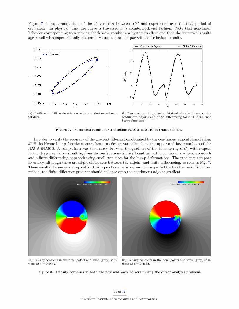
Figure 7 shows a comparison of the Cl
versus ↵ between SU2 and experiment over the final period ofoscillation. In physical time, the curve is traversed in a counterclockwise fashion. Note that non-linearbehavior corresponding to a moving shock wave results in a hysteresis e↵ect and that the numerical resultsagree well with experimentally measured values and are on par with other inviscid results.
(a) Coe�cient of lift hysteresis comparison against experimen-tal data.
(b) Comparison of gradients obtained via the time-accuratecontinuous adjoint and finite di↵erencing for 37 Hicks-Hennebump functions.
Figure 7. Numerical results for a pitching NACA 64A010 in transonic flow.
In order to verify the accuracy of the gradient information obtained by the continuous adjoint formulation,37 Hicks-Henne bump functions were chosen as design variables along the upper and lower surfaces of theNACA 64A010. A comparison was then made between the gradient of the time-averaged C
d
with respectto the design variables resulting from the surface sensitivities found using the continuous adjoint approachand a finite di↵erencing approach using small step sizes for the bump deformations. The gradients comparefavorably, although there are slight di↵erences between the adjoint and finite di↵erencing, as seen in Fig. 7.These small di↵erences are typical for this type of comparison, and it is expected that as the mesh is furtherrefined, the finite di↵erence gradient should collapse onto the continuous adjoint gradient.
(a) Density contours in the flow (color) and wave (grey) solu-tions at t = 0.1642.
(b) Density contours in the flow (color) and wave (grey) solu-tions at t = 0.2662.
Figure 8. Density contours in both the flow and wave solvers during the direct analysis problem.
15 of 17
American Institute of Aeronautics and Astronautics

To demonstrate the coupled-adjoint methodology, a single design cycle was performed for the airfoil forminimizing observed noise. The direct and adjoint problems were computed for the NACA 64A010 airfoilpitching in still air, and density contours from both the CFD and CAA solvers during the direct analysisare shown in Figure 8 for two di↵erent time steps. The airfoil was allowed to send a single pulse by pitchingupward, and the noise was computed as the square of the acoustic pressure at �
nf
. The coupled-adjoint thenprovided the time-averaged surface sensitivities to the noise, and a gradient was computed with respect tothe same 37 Hicks-Henne bump functions used above. After a single step in the gradient direction provideda new set of design variable values for the bumps, the mesh was deformed, and a new, coupled directanalysis was performed. A comparison of the baseline and deformed airfoil shapes, as well as the resultingnoise signatures versus time, are presented in Figure 9. The coupled-adjoint method successfully provided agradient that reduces the observed total noise by 1.87% after a single design cycle, mostly due to a thinningof the airfoil profile. This agrees with intuition, as a thinner airfoil should displace a smaller volume of fluidand thus produce less thickness noise.
x
y
0 0.2 0.4 0.6 0.8 1
-0.05
0
0.05
Baseline1 Design Cycle
(a) Airfoil profile comparison after one design cycle using thegradient from the coupled-adjoint to deform the Hicks-Hennebumps along the surface.
(b) Comparison of the noise amplitude over time for the base-line airfoil and the new shape after one design cycle. Thetime-average of the total noise over the interval was reducedby 1.87%.
Figure 9. Numerical results after one design cycle using the coupled continuous adjoint methodology.
VII. Conclusions
The simple demonstration of the coupled-adjoint for a pitching airfoil is just a starting point for ourinvestigation into the control of noise. This article has presented a methodology for addressing these twodisciplines via separate numerical methods coupled within a single design framework. Time-accurate contin-uous adjoint formulations have been developed for both aerodynamics and aeroacoustics, and furthermore,these formulations have been coupled through a new boundary condition which o↵ers the designer remotesensitivity information. This enables an e�cient, adjoint-based methodology for design problems involvingboth aerodynamic performance and noise control or other multidisciplinary applications featuring multiplesolvers with one-way coupling.
VIII. Acknowledgements
T. Economon would like to acknowledge U.S. government support under and awarded by DoD, Air ForceO�ce of Scientific Research, National Defense Science and Engineering Graduate (NDSEG) Fellowship, 32CFR 168a.
16 of 17
American Institute of Aeronautics and Astronautics
References
1Jameson, A., “Aerodynamic Design Via Control Theory,” AIAA 81-1259, 1981.2Jameson, A., Alonso, J. J., Reuther, J., Martinelli, L., Vassberg, J. C., “Aerodynamic Shape Optimization Techniques
Based On Control Theory,” AIAA-1998-2538, 29th Fluid Dynamics Conference, Albuquerque, NM, June 15-18, 1998.3Anderson, W. K. and Venkatakrishnan, V., “Aerodynamic Design Optimization on Unstructured Grids with a Continuous
Adjoint Formulation,” Journal of Scientific Computing, Vol. 3, 1988, pp. 233-260.4Lyrintzis, A. S., “Surface integral methods in computational aeroacoustics - From the (CFD) near-field to the (Acoustic)
far-field,” International Journal of Aeroacoustics, Vol. 2, No. 2, pp. 95-128, 2003.5Nadarajah, S. K., Jameson, A., “Optimum Shape Design for Unsteady Flows with Time-Accurate Continuous and
Discrete Adjoint Methods,” AIAA Journal, Vol. 45, No. 7, pp. 1478-1491, July, 2007.6Nielsen, E. J., Diskin, B., “Discrete Adjoint-Based Design for Unsteady Turbulent Flows On Dynamic Overset Unstruc-
tured Grids,” AIAA-2012-0554, 50th AIAA Aerospace Sciences Meeting including the New Horizons Forum and AerospaceExposition, Nashville, Tennessee, Jan. 9-12, 2012.
7Rumpfkeil, M. P., Zingg, D. W., “Unsteady Optimization Using a Discrete Adjoint Approach Applied to AeroacousticShape Design,” AIAA-2008-18, 46th AIAA Aerospace Sciences Meeting and Exhibit, Reno, NV, Jan. 7-10, 2008.
8Bueno-Orovio, A., Castro, C., Palacios, F., and Zuazua, E., “Continuous Adjoint Approach for the Spalart-AllmarasModel in Aerodynamic Optimization,” AIAA Journal , Vol. 50, No. 3, pp. 631-646, March 2012.
9Economon, T. D., Palacios, F., Alonso, J. J., “Optimal Shape Design for Open Rotor Blades,” AIAA-2012-3018, 30thAIAA Applied Aerodynamics Conference, New Orleans, Louisiana, June 25-28, 2012.
10Ffowcs Williams, J. E., Hawkings, D. L., “Sound Generation By Turbulence and Surfaces in Arbitrary Motion,” Philo-
sophical Transactions of the Royal Society of London, A 342, pp.264-321, 1969.11Alonso, J. J., Kroo, I. M., Jameson, A., “Advanced Algorithms for Design and Optimization of Quiet Supersonic Plat-
forms,” AIAA-2002-0144, 40th AIAA Aerospace Sciences Meeting and Exhibit, Reno, NV, Jan. 14-17, 2002.12Jameson, A., “Time Dependent Calculations Using Multigrid, with Applications to Unsteady Flows Past Airfoils and
Wings,” AIAA 91-1596, 10th AIAA Computational Fluid Dynamics Conference, Honolulu, Hawaii, June 24-26, 1991.13Jameson, A., Schmidt, W., and Turkel, E., “Numerical Solution of the Euler Equations by Finite Volume Methods Using
Runge-Kutta Time-Stepping Schemes,” AIAA 81-1259, 1981.14Hicks, R. and Henne, P., “Wing design by numerical optimization, Journal of Aircraft, Vol. 15, pp. 407-412, 1978.15Degand, C. and Farhat, C., “A three-dimensional torsional spring analogy method for unstructured dynamic meshes,
Computers & Structures, Vol. 80, pp. 305-316, 2002.16Davis, S. S., “NACA 64A010 (NASA Ames model) Oscillatory Pitching, Compendium of Unsteady Aerodynamic Mea-
surements, AGARD, Rept. R-702, Neuilly sur-Seine, France, Aug. 1982.
17 of 17
American Institute of Aeronautics and Astronautics