A Crash-Course on the Adjoint Method for Aerodynamic Shape ...aero.polimi.tripod.com/FilesPDF/aa200b-lect18.pdf · A Crash-Course on the Adjoint Method for Aerodynamic Shape ... AA200b

A Crash-Course on the Adjoint Method forAerodynamic Shape Optimization

Juan J. AlonsoDepartment of Aeronautics & Astronautics

Stanford [email protected]

Lecture 19

AA200b Applied Aerodynamics II, March 10, 2005 1

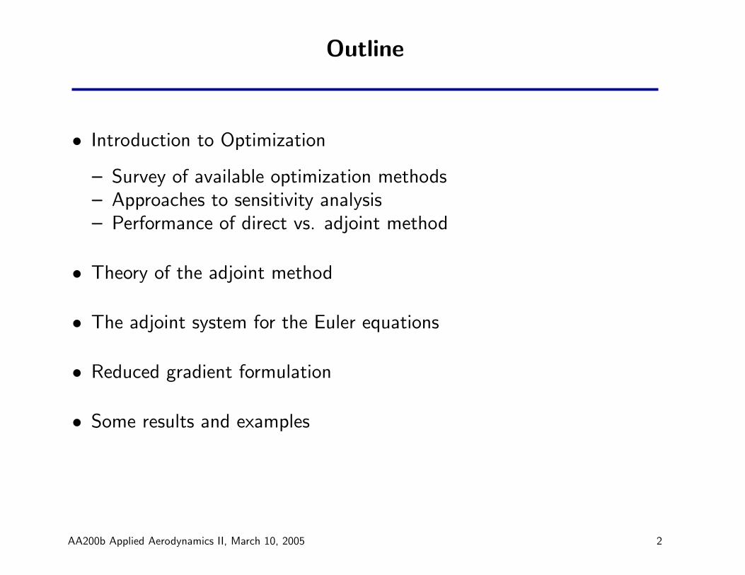
Outline

• Introduction to Optimization

– Survey of available optimization methods– Approaches to sensitivity analysis– Performance of direct vs. adjoint method

• Theory of the adjoint method

• The adjoint system for the Euler equations

• Reduced gradient formulation

• Some results and examples


Introduction to Optimization

��

��

�

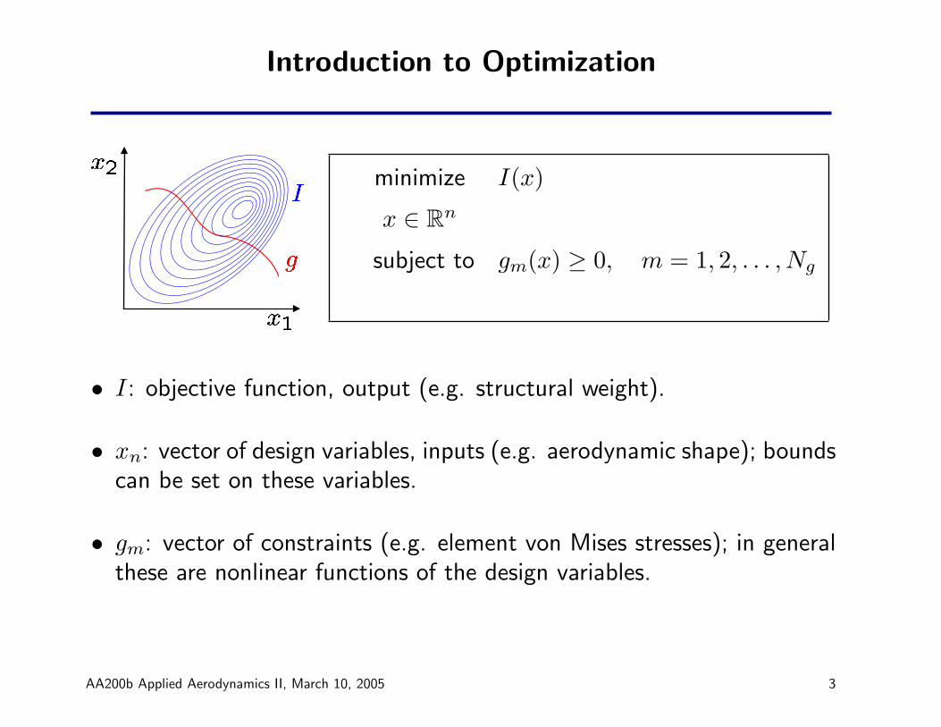
� minimize I(x)

x ∈ Rn

subject to gm(x) ≥ 0, m = 1, 2, . . . , Ng

• I: objective function, output (e.g. structural weight).

• xn: vector of design variables, inputs (e.g. aerodynamic shape); boundscan be set on these variables.

• gm: vector of constraints (e.g. element von Mises stresses); in generalthese are nonlinear functions of the design variables.


Optimization Methods

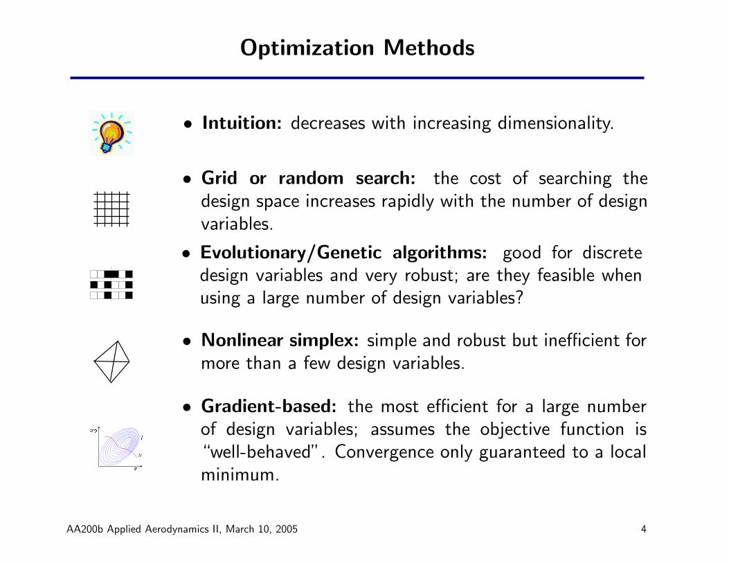
• Intuition: decreases with increasing dimensionality.

• Grid or random search: the cost of searching thedesign space increases rapidly with the number of designvariables.

• Evolutionary/Genetic algorithms: good for discretedesign variables and very robust; are they feasible whenusing a large number of design variables?

• Nonlinear simplex: simple and robust but inefficient formore than a few design variables.

��

��

�

�

• Gradient-based: the most efficient for a large numberof design variables; assumes the objective function is“well-behaved”. Convergence only guaranteed to a localminimum.


Gradient-Based Optimization: Design Cycle

��

�� !"�

#%$'&�(*)+( ,'-�.

/102/43657/

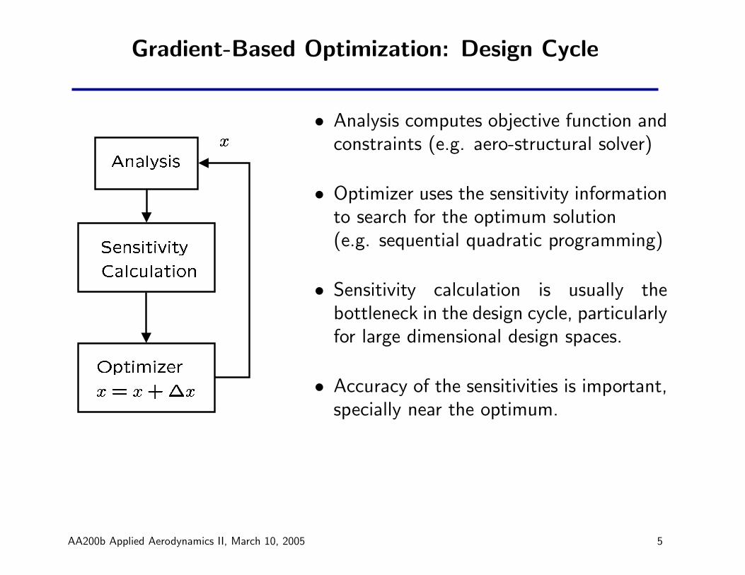
• Analysis computes objective function andconstraints (e.g. aero-structural solver)

• Optimizer uses the sensitivity informationto search for the optimum solution(e.g. sequential quadratic programming)

• Sensitivity calculation is usually thebottleneck in the design cycle, particularlyfor large dimensional design spaces.

• Accuracy of the sensitivities is important,specially near the optimum.


Sensitivity Analysis Methods

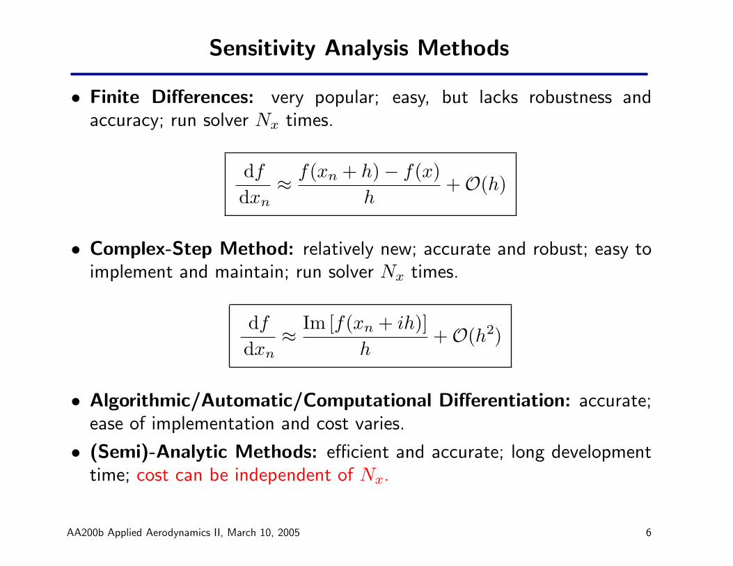
• Finite Differences: very popular; easy, but lacks robustness andaccuracy; run solver Nx times.

df

dxn≈ f(xn + h)− f(x)

h+O(h)

• Complex-Step Method: relatively new; accurate and robust; easy toimplement and maintain; run solver Nx times.

df

dxn≈ Im [f(xn + ih)]

h+O(h2)

• Algorithmic/Automatic/Computational Differentiation: accurate;ease of implementation and cost varies.

• (Semi)-Analytic Methods: efficient and accurate; long developmenttime; cost can be independent of Nx.


Finite-Difference Derivative Approximations

From Taylor series expansion,

f(x + h) = f(x) + hf ′(x) + h2f′′(x)2!

+ h3f′′′(x)3!

+ . . . .

Forward-difference approximation:

⇒ df(x)dx

=f(x + h)− f(x)

h+O(h).

f(x) 1.234567890123484

f(x + h) 1.234567890123456

∆f 0.000000000000028

x x+h

f(x)

f(x+h)


Complex-Step Derivative Approximation

Can also be derived from a Taylor series expansion about x with a complexstep ih:

f(x + ih) = f(x) + ihf ′(x)− h2f′′(x)2!

− ih3f′′′(x)3!

+ . . .

⇒ f ′(x) =Im [f(x + ih)]

h+ h2f

′′′(x)3!

+ . . .

⇒ f ′(x) ≈ Im [f(x + ih)]h

No subtraction! Second order approximation.


Simple Numerical Example

Step Size, h

Norm

aliz

ed E

rror,

e

Complex-StepForward-DifferenceCentral-Difference

Estimate derivative atx = 1.5 of the function,

f(x) =ex

√sin3x + cos3x

Relative error defined as:

ε =

∣∣∣f ′ − f ′ref

∣∣∣∣∣∣f ′ref

∣∣∣


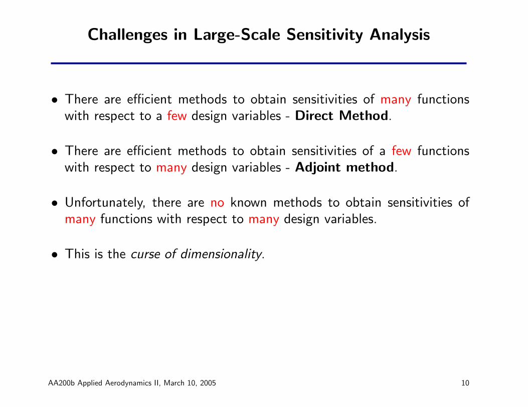
Challenges in Large-Scale Sensitivity Analysis

• There are efficient methods to obtain sensitivities of many functionswith respect to a few design variables - Direct Method.

• There are efficient methods to obtain sensitivities of a few functionswith respect to many design variables - Adjoint method.

• Unfortunately, there are no known methods to obtain sensitivities ofmany functions with respect to many design variables.

• This is the curse of dimensionality.


Outline








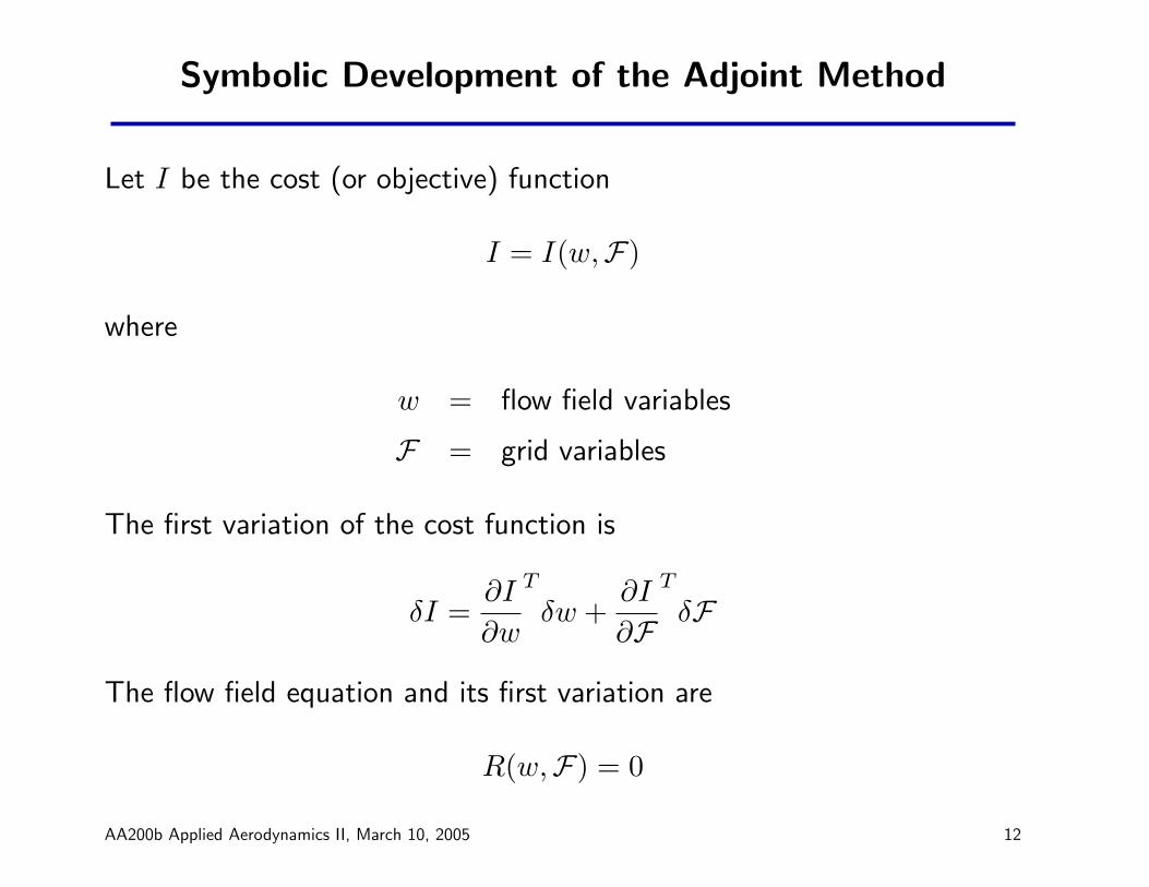
Symbolic Development of the Adjoint Method

Let I be the cost (or objective) function

I = I(w,F)

where

w = flow field variables

F = grid variables

The first variation of the cost function is

δI =∂I

∂w

T

δw +∂I

∂FT

δF

The flow field equation and its first variation are

R(w,F) = 0


δR = 0 =[∂R

∂w

]δw +

[∂R

∂F]

δFIntroducing a Lagrange Multiplier, ψ, and using the flow field equation asa constraint

δI =∂I

∂w

T

δw +∂I

∂FT

δF − ψT

{[∂R

∂w

]δw +

[∂R

∂F]

δF}

=

{∂I

∂w

T

− ψT

[∂R

∂w

]}δw +

{∂I

∂FT

− ψT

[∂R

∂F]}

δF

By choosing ψ such that it satisfies the adjoint equation

[∂R

∂w

]T

ψ =∂I

∂w,

we have

δI =

{∂I

∂FT

− ψT

[∂R

∂F]}

δF


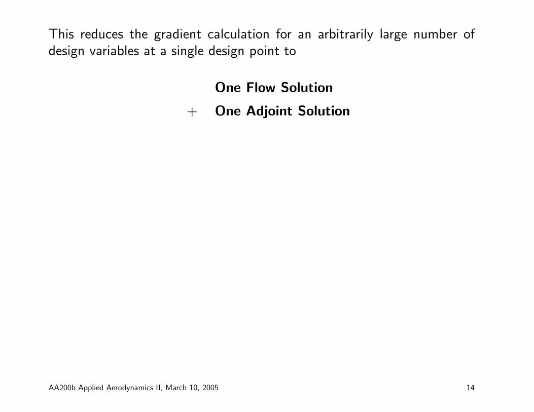
This reduces the gradient calculation for an arbitrarily large number ofdesign variables at a single design point to

One Flow Solution

+ One Adjoint Solution


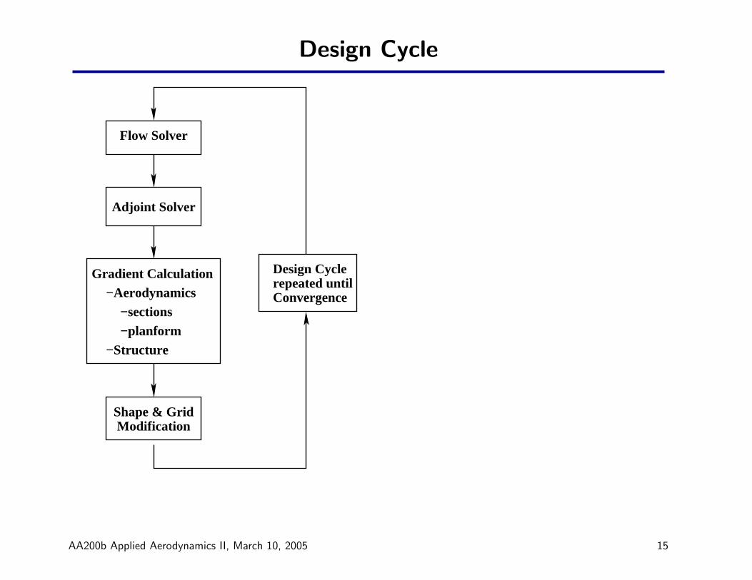
Design Cycle

−sections−planform

Shape & GridModification

repeated untilConvergence

Design Cycle

Flow Solver

Adjoint Solver

Gradient Calculation−Aerodynamics

−Structure


Outline








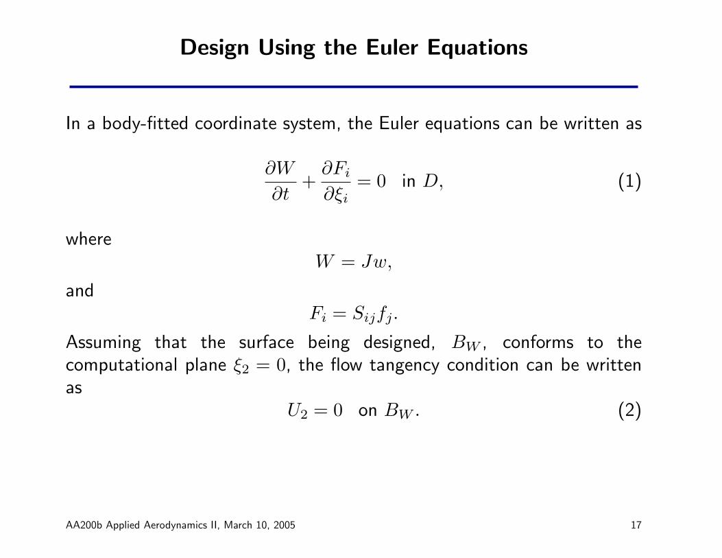
Design Using the Euler Equations

In a body-fitted coordinate system, the Euler equations can be written as

∂W

∂t+

∂Fi

∂ξi= 0 in D, (1)

whereW = Jw,

andFi = Sijfj.

Assuming that the surface being designed, BW , conforms to thecomputational plane ξ2 = 0, the flow tangency condition can be writtenas

U2 = 0 on BW . (2)


Formulation of the Design Problem

Introduce the cost function

I =12

∫ ∫

BW

(p− pd)2dξ1dξ3.

A variation in the shape will cause a variation δp in the pressure andconsequently a variation in the cost function

δI =∫ ∫

BW

(p− pd) δp dξ1dξ3. (3)

Since p depends on w through the equation of state the variation δp canbe determined from the variation δw. Define the Jacobian matrices

Ai =∂fi

∂w, Ci = SijAj. (4)


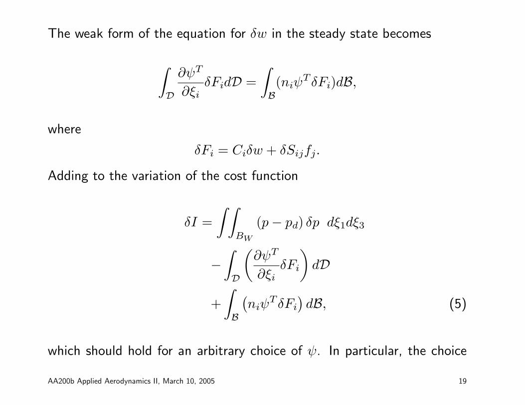
The weak form of the equation for δw in the steady state becomes

∫

D

∂ψT

∂ξiδFidD =

∫

B(niψ

TδFi)dB,

where

δFi = Ciδw + δSijfj.

Adding to the variation of the cost function

δI =∫ ∫

BW

(p− pd) δp dξ1dξ3

−∫

D

(∂ψT

∂ξiδFi

)dD

+∫

B

(niψ

TδFi

)dB, (5)

which should hold for an arbitrary choice of ψ. In particular, the choice


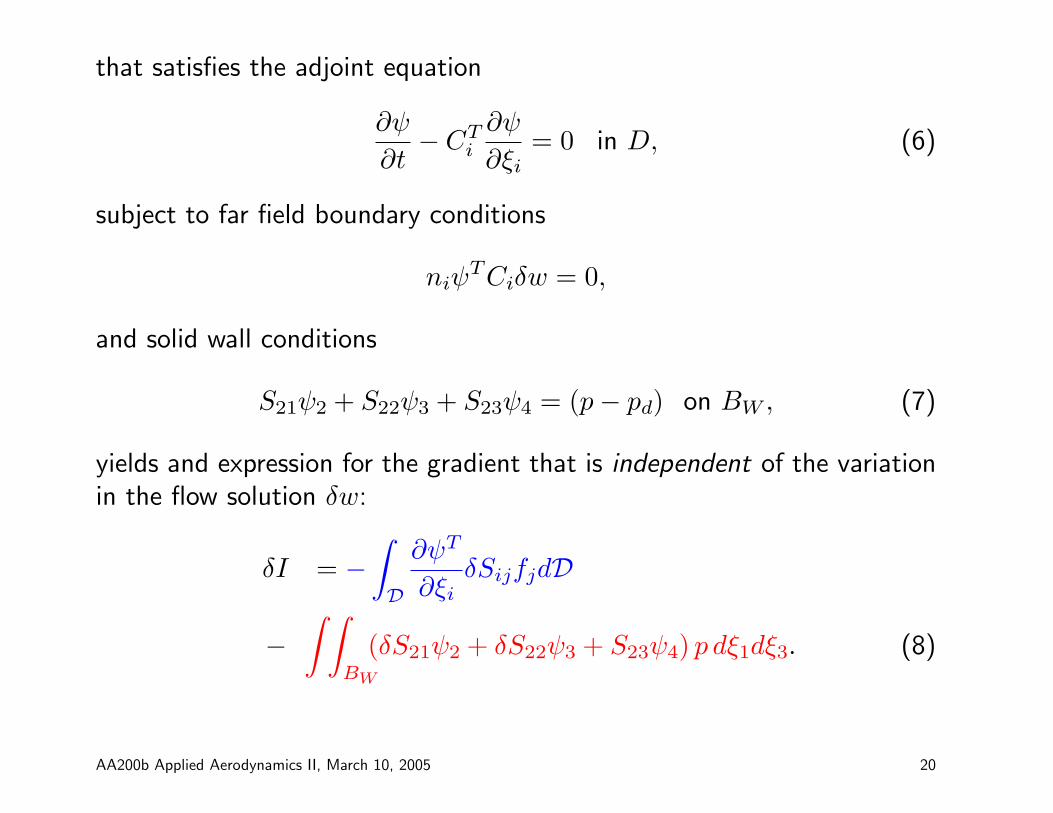
that satisfies the adjoint equation

∂ψ

∂t− CT

i

∂ψ

∂ξi= 0 in D, (6)

subject to far field boundary conditions

niψTCiδw = 0,

and solid wall conditions

S21ψ2 + S22ψ3 + S23ψ4 = (p− pd) on BW , (7)

yields and expression for the gradient that is independent of the variationin the flow solution δw:

δI = −∫

D

∂ψT

∂ξiδSijfjdD

−∫ ∫

BW

(δS21ψ2 + δS22ψ3 + S23ψ4) p dξ1dξ3. (8)


Outline








The Reduced Gradient Formulation

Consider the case of a field mesh variation with a fixed boundary. Then,

δI = 0,

but there is a variation in the transformed flux,

δFi = Ciδw + δSijfj.

Here the true solution is unchanged, so the variation δw is due to thefield mesh movement δx. Therefore

δw = ∇w · δx =∂w

∂xjδxj (= δw∗) ,

and since∂

∂ξiδFi = 0,


it follows that

∫

DψT ∂

∂ξi(δSijfj) dD = −

∫

DψT ∂

∂ξi(Ciδw

∗) dD. (9)

A similar relationship has been derived in the general case with boundarymovement and the complete derivation will be presented in un upcomingconference paper. Now

∫

DψTδRdD =

∫

DψT ∂

∂ξiCi (δw − δw∗) dD

=∫

BψTCi (δw − δw∗) dB

−∫

D

∂ψT

∂ξiCi (δw − δw∗) dD. (10)

By choosing ψ to satisfy the adjoint equation (6) and the adjoint boundary


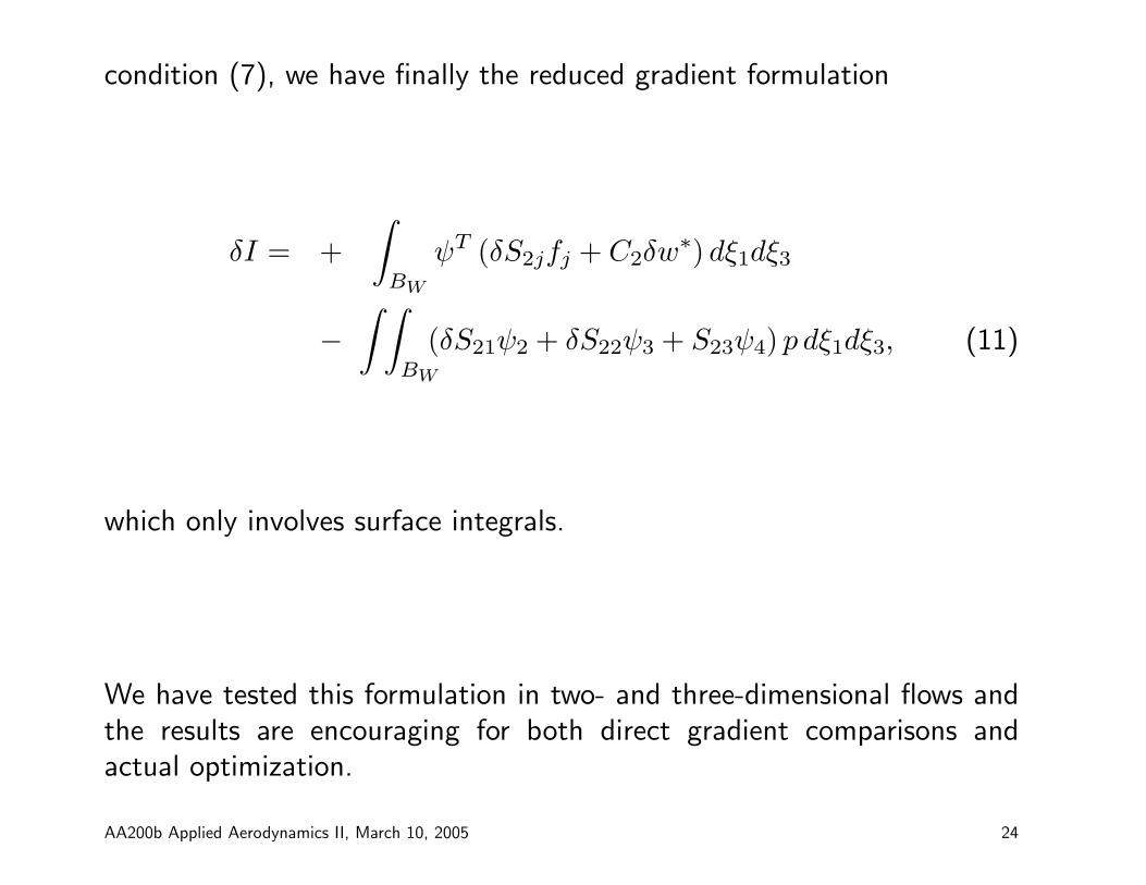
condition (7), we have finally the reduced gradient formulation

δI = +∫

BW

ψT (δS2jfj + C2δw∗) dξ1dξ3

−∫ ∫

BW

(δS21ψ2 + δS22ψ3 + S23ψ4) p dξ1dξ3, (11)

which only involves surface integrals.

We have tested this formulation in two- and three-dimensional flows andthe results are encouraging for both direct gradient comparisons andactual optimization.


0 20 40 60 80 100 120 140−0.5

−0.4

−0.3

−0.2

−0.1

0

0.1

0.2

0.3

0.4Comparison of Adjoint and Finite Difference Gradients

Number of Control Parameter ( Bump Using 3 Mesh Points)

Gra

dien

ts

Original AdjointReduced AdjointFinite−Difference

Figure 1: Euler Drag Minimization for RAE2822: Comparison ofOriginal Adjoint, Reduced Adjoint and Finite-Difference Gradients Using3 Mesh-Point Bump as Design Variable.


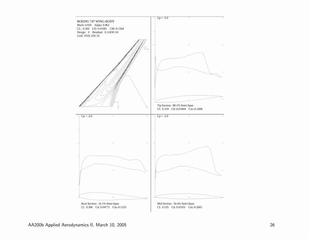
BOEING 747 WING-BODY Mach: 0.930 Alpha: 0.962 CL: 0.360 CD: 0.01681 CM:-0.1564 Design: 0 Residual: 0.1245E+01 Grid: 193X 33X 33

Cl: 0.306 Cd: 0.04773 Cm:-0.1533 Root Section: 16.1% Semi-Span

Cp = -2.0

Cl: 0.535 Cd: 0.01931 Cm:-0.2665 Mid Section: 50.4% Semi-Span

Cp = -2.0

Cl: 0.319 Cd:-0.01804 Cm:-0.1608 Tip Section: 88.1% Semi-Span

Cp = -2.0


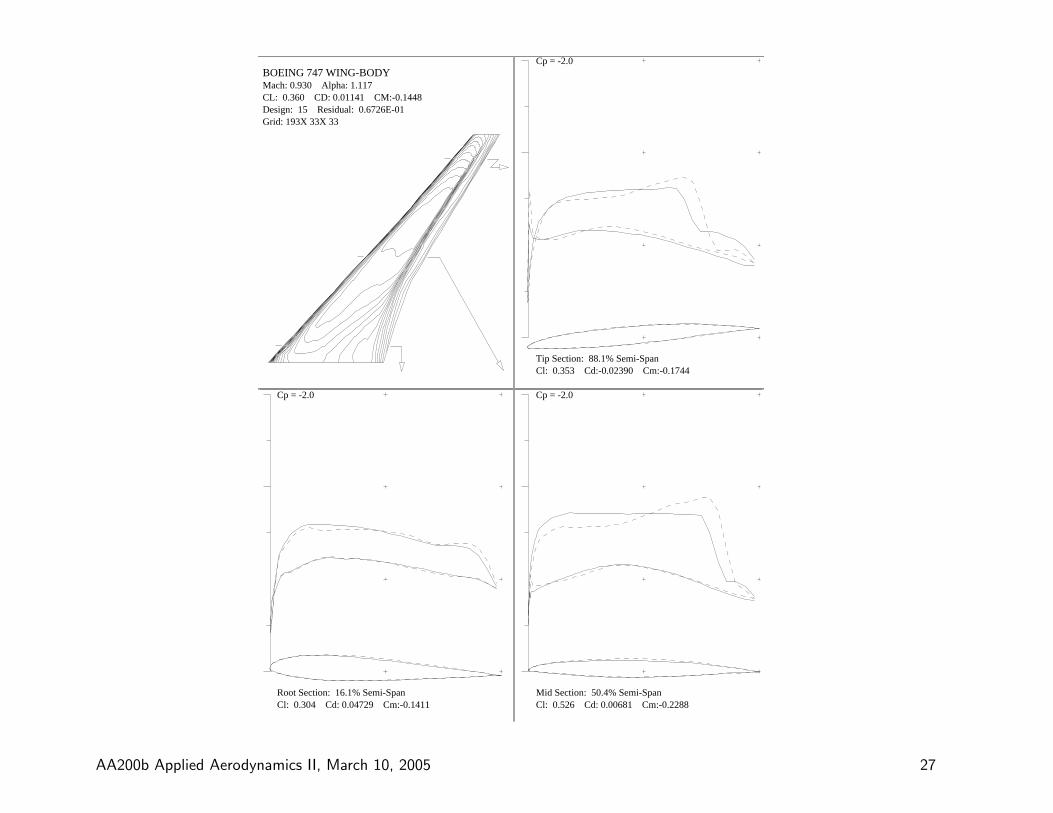
BOEING 747 WING-BODY Mach: 0.930 Alpha: 1.117 CL: 0.360 CD: 0.01141 CM:-0.1448 Design: 15 Residual: 0.6726E-01 Grid: 193X 33X 33

Cl: 0.304 Cd: 0.04729 Cm:-0.1411 Root Section: 16.1% Semi-Span

Cp = -2.0

Cl: 0.526 Cd: 0.00681 Cm:-0.2288 Mid Section: 50.4% Semi-Span

Cp = -2.0

Cl: 0.353 Cd:-0.02390 Cm:-0.1744 Tip Section: 88.1% Semi-Span

Cp = -2.0


Adjoint Design Software

The adjoint for the Euler and Navier-Stokes equations has beenimplemented into the following codes:

• SYN87: Wing-alone Euler C-H mesh.

• SYN88: Wing-body Euler C-H mesh.

• SYN107: Wing-body N-S C-H mesh.

• SYN87-MB: Arbitrary configuration, Euler, multiblock mesh.

• SYN107-MB: Arbitrary configuration, N-S, multiblock mesh.

• SYNPLANE: Arbitrary configuration, Euler, unstructured mesh.


Adjoint Design Projects

Adjoint methods (Euler and/or N-S) have been used with the followingconfigurations:

• Boeing 747-200

• McDonnell Douglas MDXX

• Raytheon Premier I

• NASA High Speed Civil Transport

• Reno Air Racer

• IPTN N2130

• Other projects at BAE, DLR, NLR, etc.

• Research configurations (subsonic, transonic, supersonic)


Documents

A Crash-Course on the Adjoint Method for Aerodynamic Shape ...aero.polimi.tripod.com/FilesPDF/aa200b-lect18.pdf · A Crash-Course on the Adjoint Method for Aerodynamic Shape ... AA200b