A control-theoretical methodology

for the scheduling problem

Carlo A. Furia · Alberto Leva · Martina Maggio · Paola Spoletini

Abstract

This paper presents a novel methodology to develop scheduling algo-rithms. The scheduling problem is phrased as a control problem, andcontrol-theoretical techniques are used to design a scheduling algorithmthat meets specific requirements. Unlike most approaches to feedbackscheduling, where a controller integrates a “basic” scheduling algorithmand dynamically tunes its parameters and hence its performances, ourmethodology essentially reduces the design of a scheduling algorithm tothe synthesis of a controller that closes the feedback loop. This ap-proach allows the re-use of control-theoretical techniques to design efficientscheduling algorithms; it frames and solves the scheduling problem in ageneral setting; and it can naturally tackle certain peculiar requirementssuch as robustness and dynamic performance tuning. A few experimentsdemonstrate the feasibility of the approach on a real-time benchmark.

1 Introduction

The word scheduling refers to the allocation of resources between different com-peting tasks. This generic, abstract definition reflects the pervasiveness of thescheduling concern across disciplinary fields. A concrete class of schedulingproblems is obtained by specifying a type of system and tasks, and the goals ofthe scheduling action.

In this paper, we outline a general methodology to tackle the schedulingproblem. Our approach exploits control theory to formulate the schedulingproblem and to solve it. The control-theoretical paradigm represents the in-teraction between two distinct parts of a system: the plant and the controller.The plant represents the part of the system whose dynamics is not modifiabledirectly, and that must be put under control. The controller, on the other hand,is a component that provides suitable input to the plant with the goal of influ-encing its dynamics towards meeting some requirements. The controller choosesits action according to the output of the plant, hence the denomination feedbackcontrol.

The idea of using control theory to solve scheduling problems is not new.Indeed, the research area of feedback scheduling is based on these premises [11, 5].The novelty of our approach consists in how the control-theoretical paradigm isapplied to the scheduling problem, and more precisely which parts of the systemare modeled as the plant and as the controller, respectively.

The most common approach to feedback scheduling supplements an existingscheduler with a control-theoretical model: the plant is the “basic” scheduler

1

arX

iv:1

009.

3455

v1 [

cs.S

Y]

17

Sep

2010

itself, and the controller tunes its dynamics over time according to the evolu-tion of the rest of the system. We suggest a different partitioning, where thecontroller is the scheduler and the plant is a very abstract model of the pool oftasks and, in some sense, the resources they run on.

Our stance has a couple of significant advantages over the traditional ap-proaches. First, it allows the effective re-use of an extensive amount of powerfulresults from classical control theory to smoothly design scheduling algorithms.Second, it is remarkably flexible and can easily accommodate some complexand peculiar scheduling requirements, such as robustness towards disturbances,dynamic adjustment of performance, and a quantitative notion of convergencerates.

The approach is general and applies to a large class of scheduling problems.It is naturally applicable to scheduling the CPU in real-time systems [14, 8],which are characterized by a quantitative treating of time. As it is commonwith feedback scheduling, it focuses on soft real-time, where the failure to re-spect a deadline does not result in a global failure of the system, and averageperformance is what matters.

The heterogeneous scope of the scheduling problem and the sought gener-ality of the present approach make, at times, the presentation of the technicaldetails necessarily abstract: it is impossible to formalize each and every (domain-specific) aspect of the scheduling problem (e.g., deadlines, priorities, granular-ities, etc.) in a unique model that is practically useful. Additionally, differentformalizations are often possible, and choosing the best one depends largely onapplication-specific details, such as whether one is dealing with a batch or ahard real-time system. The overall goal of the present paper is high-level: out-lining the framework proposed, formalizing its basic traits, and demonstratingits flexibility with a few examples. Focusing the framework on specialized classesof scheduling problems and comparatively assessing its performance belongs tofuture work.

The rest of the paper presents our approach to feedback scheduling and isorganized as follows. Section 2 presents some additional motivation, with a moredirect comparison to the literature which is most closely related to this paper.Section 3 introduces our methodology for the scheduling problem; it focuses onpresenting the conceptual contribution in a general setting. Section 4 discussesan experimental validation of the approach, where the general methodology isinstantiated to solve a few specific concrete problems in a real-time schedulingbenchmark. Finally, Section 5 draws some conclusions and outlines future work.

2 Motivation and related work

Hellerstein et al.’s book [4] is a comprehensive review of the applications ofcontrol theory to computing-system problems such as bandwidth allocation andunpredictable data traffic management. In general, control theory is applied tomake computing systems adaptive, more robust, and stable. Adaptability, inparticular, characterizes the response required in applications whose operatingconditions change rapidly and unpredictably.

Lu et al. [9, 10] present contributions in this context, for the regulation of theservice levels of a web server. The variable to be controlled is the delay betweenthe arrival time of a request and the time it starts being processed. The goal is

2

to keep this delay to within some desired range; the range depends on the classof each request. An interesting point of this works is the distinction betweenthe transient and steady state performances, in the presence of variable traffic.This feature motivates a feedback-control approach to many computing-systemperformance problems.

Scheduling is certainly one of these problems where the transient to steady-state distinction features strongly. Indeed, many ad hoc scheduling approachessolve essentially the same problem in different operating conditions. This isone of the main reasons why feedback scheduling has received much attention inrecent years (see Xia and Sun [19] for a concise review of the topic). As we ar-gued already in the introduction, the standard approach in feedback schedulingconsists in “closing some control loop around an existing scheduler” to adjustits parameters to the varying load conditions. This may yield performanceimprovements, but it falls short of fully exploiting the rich toolset of controltheory.

For example, in Abeni et al. [1], the controller adjusts the reservation time(i.e., the time the scheduler assigns to each task) with the purpose of keepingthe system utilization below a specified upper bound. The plant is instead aswitching system with two different states, according to whether the systemcan satisfy the total amount of CPU requests or not. Some tests with a real-time Linux kernel show that the adaptation mechanism proposed is useful forto improve quality-of-service measurements. Continuing in the same line ofwork, Palopoli and Abeni [12] combine a reservation-based scheduler and afeedback-based adaptation mechanism to identify the best parameter set for agiven workload. Block et al. pursue a similar approach [2] where they integratefeedback models with optimization techniques.

In Lawrence et al. [7], the controller adjusts the reservation time to within anupper bound given by the most frequently activated task. The model of the plantis a continuous-time system whose variables record the queuing time of tasks.The effectiveness of the method proposed is validated through simulations.

Lu et al. in [11] consider some basic scheduling policies (both open-loop andclosed-loop) and design a controller that prevents system overloading. Such goalis achieved by letting some tasks out of the queue when the system workload istoo high.

All these approaches target the same problem: assigning CPU time to apool of tasks to meet some goals. The devised algorithms are usually extremelyefficient, but their scope of applicability is often limited to a fairly specific do-main (e.g., periodic processes with harmonic frequencies deadlines). Moreover,in all the cited approaches the controller modifies the behavior of a “basic”scheduling algorithm; indeed, the model of the scheduler is often combined with(some aspects) of the processor model, even if their functions are in principleclearly distinct. We believe that this lack of separation of concerns is the resultof the close adherence to a specific scheduling problem domain, and we claimthat enforcing a stricter separation in the model can result in some distinctiveadvantage.

The rest of the paper presents an approach where the scheduler is solely re-sponsible for selecting which tasks have to run and their desired execution time.The scheduler is then built as the controller that meets some requirements forsuch a selection. Notice that the homogeneous nature of the controller (i.e., thescheduler) and the plant (i.e., the tasks’ execution model) is peculiar to com-

3

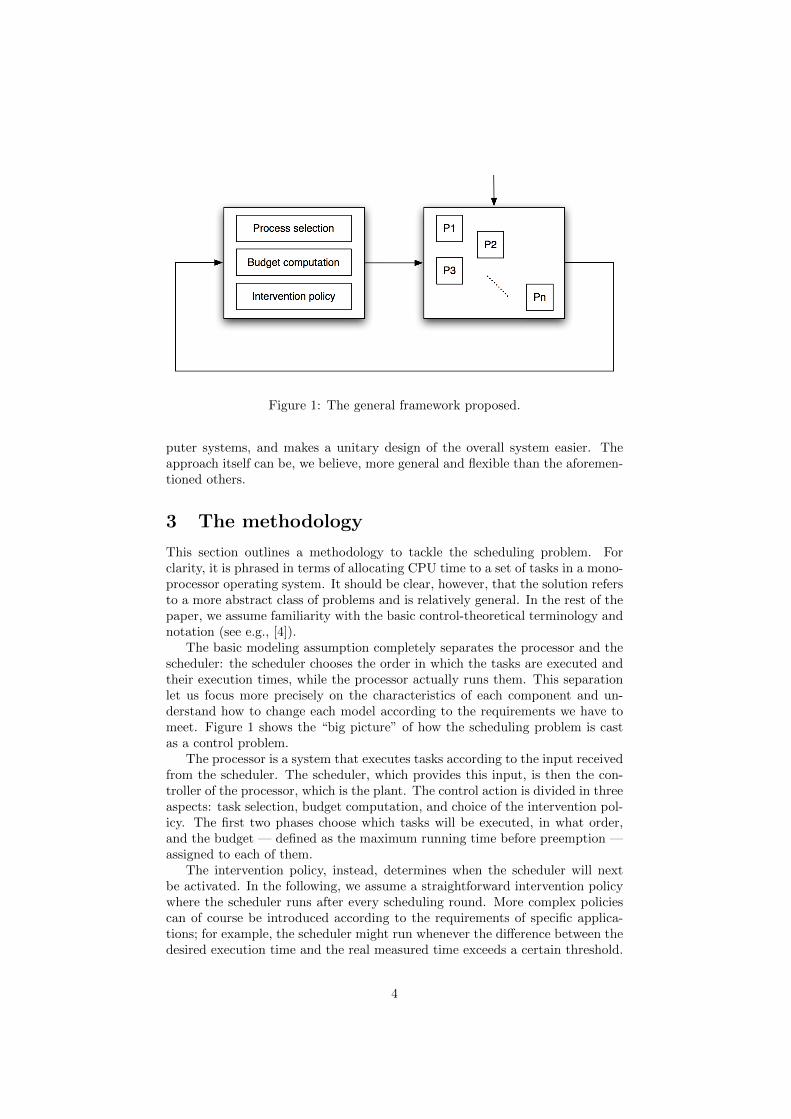
Figure 1: The general framework proposed.

puter systems, and makes a unitary design of the overall system easier. Theapproach itself can be, we believe, more general and flexible than the aforemen-tioned others.

3 The methodology

This section outlines a methodology to tackle the scheduling problem. Forclarity, it is phrased in terms of allocating CPU time to a set of tasks in a mono-processor operating system. It should be clear, however, that the solution refersto a more abstract class of problems and is relatively general. In the rest of thepaper, we assume familiarity with the basic control-theoretical terminology andnotation (see e.g., [4]).

The basic modeling assumption completely separates the processor and thescheduler: the scheduler chooses the order in which the tasks are executed andtheir execution times, while the processor actually runs them. This separationlet us focus more precisely on the characteristics of each component and un-derstand how to change each model according to the requirements we have tomeet. Figure 1 shows the “big picture” of how the scheduling problem is castas a control problem.

The processor is a system that executes tasks according to the input receivedfrom the scheduler. The scheduler, which provides this input, is then the con-troller of the processor, which is the plant. The control action is divided in threeaspects: task selection, budget computation, and choice of the intervention pol-icy. The first two phases choose which tasks will be executed, in what order,and the budget — defined as the maximum running time before preemption —assigned to each of them.

The intervention policy, instead, determines when the scheduler will nextbe activated. In the following, we assume a straightforward intervention policywhere the scheduler runs after every scheduling round. More complex policiescan of course be introduced according to the requirements of specific applica-tions; for example, the scheduler might run whenever the difference between thedesired execution time and the real measured time exceeds a certain threshold.

4

A detailed analysis of this aspect is orthogonal to the rest of our methodologyand belongs to future work.

Separating the scheduler action in three components facilitates modificationsof the controller model according to different requirements. More precisely, theoverall model structure remains the same and only the equations modeling theaffected aspects need to be changed.

Notice that anything that influences the behavior of the running tasks, otherthan the scheduler action, is modeled as an exogenous disturbance: an actionthat prevents the system from reaching the goal requirements, which the sched-uler wants to contrast. This modeling assumption is suitable for factors that are,for all practical purposes, unpredictable and unmodifiable. The notion of dis-turbance (basically disturbance rejection) from control theory is then adoptedto model these factors, with the immediate benefit of having at our disposal apowerful set of theoretical tools to tackle effectively the ensuing problems.

The abstractness and genericity of our framework come with the potentialdrawback of making it difficult to implement the scheduling policies within anexisting scheduler architecture, which can differ significantly from the abstractmodular structure of Figure 1. Anyway, we believe that the theoretical analysisthat can be carried out within our framework is extremely useful to determinethe criticalities of the system under design, even in the cases in which the finalimplementation will require ad hoc adjustments.

3.1 The plant

The “open loop” model of the plant describes the process executor as a discrete-time system. It receives a schedule (which will be the output of the schedulerdescribed in the next subsection) as input and returns the outcome of executingthe tasks as required by the schedule.

A round is the time between two consecutive runs of the scheduler. As-sume that more than one task can be scheduled for execution in a given round;correspondingly, we introduce the following variables to describe the plant:

• N , the number of tasks to be scheduled;

• τp(k) ∈ RN , the actual running times of the tasks in the k-th schedulinground;

• τr(k) ∈ R, the duration of the k-th round;

• s(k) ∈ RN , the schedule at the k-th round: an ordered list of the budgets,one for each task; the order determines the execution order and a budgetof 0 means that the task is not scheduled for execution in that round;

• δb(k) ∈ RN , the disturbance during the k-th round, defined as the differ-ence between the assigned budget and the actual running time of a task;(Notice that this variable models uniformly a variety of possible specificphenomena, such as a task that yields control or terminates before pre-emption, an interrupt occurring, the execution of a critical section wherepreemption was disabled, etc.)

• t ∈ R, the total time actually elapsed from the system initialization.

5

The model of the plant is then the following system of equations: τp(k) = s(k − 1) + δb(k − 1)τr(k) = r1τp(k − 1)t(k) = t(k − 1) + τr(k − 1)

(1)

where r1 is a row vector of length N with all unit elements.Model (1) is linear and time-invariant. Negative budgets are not allowed

and, correspondingly, each s(k) + δb(k) element cannot be negative. However,this is irrelevant for the controller, since the set of considered variables is smallerthan the domain limitations. Notice that the discrete-time model assumes thatthe scheduler is active only once per round. Clearly, some s(k) elements can bezero, meaning that not all the tasks will actually run. The τr variable modelsround duration, which takes into account system responsiveness issues.

3.2 The scheduler

A scheduler should usually achieve the following goals, regardless of the speci-ficities of the system where it runs [16].

• Fairness: comparable tasks should get comparable service; (This obvi-ously does not apply to tasks with different properties.)

• Policy enforcement : the scheduler has to comply to general system poli-cies; (This aspect is especially relevant for real-time systems where con-straining system policies are usually in place.)

• Balance: all the components of the system need to be used as uniformlyas possible.

In addition to these general requirements, a scheduler must also achieve ad-ditional goals that are specific to the system at hand. For instance, in batchsystems, where responsiveness is not an issue, the scheduler should guaranteemaximization of the throughput, minimization of the turnaround time, andmaximization of CPU utilization. In interactive systems, on the contrary, min-imization of response time and proportionality guarantees are likely schedulinggoals. Finally, deadlines and predictability are specific to real-time systems.

In the following, we outline a general approach to design a scheduler —based on control-theory and the framework presented above — that achieves adefined set of goals. Unlike the standard approach that designs a new algorithmfor a new class of systems, we can accommodate most scenarios within the sameframework by changing details of the equations describing the control model.

Process selection and budget computation. The scheduler decideswhich tasks to activate and chooses a budget for them. This is achieved bysetting variable si(k) which defines the budget assigned to the i-th task atround k. This action is actually made of two conceptually different parts. AProcess Selection Component (PSC) takes care of deciding the next task tobe executed by the processor, while a Budget Computation Component (BCC)fixes the duration of the execution for each selected task. If more than one taskis to be executed per round, PSC computes an ordered list of tasks and BCCassigns one or more budgets to the elements of the list. Execution need not be

6

continuous: if a time ti is assigned to the i-th task, the actual execution can besplit into multiple slots within the same round.

The distinction between PSC and BCC is modeled by defining s(k) asSσ(k) b(k), where Sσ(k) is a N × n(k) matrix representing the tasks selectedat the k-th round, while b(k) ∈ Rn(k) represents the budget assigned to theselected tasks. Notice that, in the most general case, the number of tasks thatcan be executed at each round is a variable n(k).

PSC can operate statically or dynamically. In the first case, the strategy isindependent of the previous choices, such as in Round Robin (RR) scheduling.In the second case, PSC retains a history of the previous choices and bases itsnew choice on it, such as in fair-share scheduling [6].

In case of static PSC, the matrix Sσ(k) is not explicitly function of b(i) andSσ(j), with i, j < k. This means that Sσ(k) may not be a function of both τpand τr in the previous rounds; indeed, these represent the actual behavior of theCPU with respect to each task. Therefore, they may not reflect the choice thatthe scheduler made in previous rounds, due to contingencies in the executionof the system. Consider, as a more concrete example, the shortest remainingtime next algorithm: the PSC chooses the next task to be executed accordingto their remaining running times, which obviously depend on what actuallyhappened in the previous rounds (i.e., the history of τp), but not necessarily onthe scheduler’s choice (i.e., s).

Once the PSC has selected the tasks to be executed, the BCC computes thebudgets for them, by setting b(k). PSC can be static or dynamic, too: in the

first case the budget is a constant vector b(k) = b, whereas in the second casethe budget may change at every round.

Designing the controller. Let us now discuss how to define and enforcesome of the previously outlined features in a scheduler, for given PSC and BCC.

3.2.1 Fairness

A fair scheduling algorithm has the property that, in every fixed time interval,the CPU usage is proportionally distributed among tasks, accordingly to theirweights. For the sake of simplicity, let us focus on a fixed number of rounds H.1

Let pi(k) be the weight of the i-th task at the k-th round. In order to guaranteefairness for each task, the scheduler must achieve the following equation:

k+H∑i=k

τpi(k) =

k+H∑i=k

pi(k)∑Nj=1 pj(k)

τr(k) (2)

Informally, (2) means that the scheduler distributes the CPU among the dif-ferent tasks proportionally to their weights (over the next H rounds). Then,the scheduler computes a s(k) which satisfies equation (2). The algorithm tocompute s(k) comes from the solution to the corresponding control problem,for example by means of optimal control theory2: find the optimal value of thecontrolled variable s(k), given a certain cost function J of the state variablesτp, τr, t.

1Generalizing this approach to deal with a time window, rather than a number of rounds,is straightforward.

2See [3] for an overview of optimal control theory and further references on the subject.

7

3.2.2 Policy enforcement

The details of how to handle this aspect within our control framework dependessentially on which system policy should be enforced: the term “policy” canrefer to very disparate concerns. The experiments described in Section 4 willtackle a specific instance of activation policy.

Let us notice, in passing, that the strict coupling between the system policyand the features of the controller that enforce such a policy is one of the reasonswhy most scheduling algorithms do not disentangle the different aspects andtend to lump all of them together in the same model.

3.2.3 Balance

Balance requirements do not belong to the simplified model of equation (1),which refers to a mono-processor system whose only resource is CPU time.It is straightforward, however, to extend the model along the same lines toaccommodate additional resources, such as another CPU or I/O bandwidth.New variables would model the usage of these further resources, with the sameassumptions as in (1). Of course, these control variables must be measurablein the real system for the scheduler to be effectively implementable (see [5] fora discussion of this orthogonal aspect). Then, control-theoretical techniques —such as optimal control theory or model-predictive control — can be used todesign a scheduler which enforces a resource occupation given as a set point.

3.2.4 Throughput maximization

If throughput is part of the requirements for our scheduler, we include thefollowing set of equations in the model (1):

ρp(k) = max (ρp(k − 1)− τp(k − 1), 0) (3)

Equation (3) defines ρp(k), the remaining execution time of task p at round k,as the difference between the remaining time during the previous round and theactual running time of p during the current round. Throughput maximizationcan then be defined as the round-wise maximization of the number of processeswhose ρp value is zero. Standard control-theoretical techniques can then designa controller that provably achieves this requirement.

3.2.5 Responsiveness

The model (1) includes a variable τr that describes the duration of a round,hence requirements on the response time can be expressed as a target value forτr. More precisely, the smaller τr, the more responsive is the controlled system.

3.2.6 Other requirements

The same framework can address other requirements, such as turnaround time,CPU utilization, predictability, proportionality, and deadline enforcement. Asan example, the experiments in Section 4 will address proportionality and dead-line enforcement explicitly.

8

3.3 Complexity parameters

Analyzing the complexity of scheduling algorithms is often arduous, mostly dueto the difficulty of determining the right level of abstraction to describe thevarious components (i.e., the processor, the scheduler, etc.). It also does notmake sense to compare directly the general framework we have outlined to exist-ing algorithms; on the contrary, specific implementations can be experimentallyevaluated.

It is nonetheless interesting to present a few simple rules of thumb to have arough estimate of the complexity of an algorithm designed within our framework.With the goal of determining the number of elementary operations spent by theCPU to execute the scheduling algorithm itself, let us introduce the constantstΣ, tS , tΠ, and t→. They denote the (average) duration of a sum, subtraction,multiplication, and bit-shift operation, respectively. Also, let tc denote the(average) duration of a “light” context switch (i.e, the time overhead taken byoperations such as storing and restoring context information, which does notinclude the actual computation of the next task to be run and its budget).Using these figures, Section 4 evaluates the complexity of a specific algorithmthat validates our framework.

4 Application and experimental results

This section instantiates the framework proposed by developing a schedulerwith certain proportionality and deadline meeting requirements with control-theoretic techniques. The design is evaluated on the Hartstone [18, 17] bench-mark, a standard real-time system benchmark. The Hartstone benchmark eval-uates deadline misses and was initially conceived to assess architectures andcompilers, but it can be used also for evaluating the performances of a schedul-ing algorithm.

The design and the evaluation are necessarily preliminary, and do not tackleevery aspect that is relevant in real-time scheduling (for example, earliness/tardinessbounds are not considered); these experiments are meant as a feasibility demon-stration of the approach and tackling more challenging problems belongs tofuture work.

Regulating round duration and CPU distribution. One of the re-quirements fixes a desired duration for scheduling rounds; let τ◦r denote such aduration. Moreover, define

θ◦p ∈ RN , θ◦p,i ≥ 0,

N∑i=1

θ◦p,i = 1 (4)

as the vector with the fractions of CPU time to be allotted to each task. Thisvector can be expressed as a function of workload and round duration, andthe corresponding requirement be expressed as a set point for each task. Moregenerally, notice that requirements on fairness, tardiness, and similar features,are also expressible in terms of τ◦r and θ◦p.

Let us now show a possible approach to design a scheduler that meets therequirement on the duration of the scheduling rounds. Consider for example acascade controller such as in Figure 2. An appropriate choice for the involved

9

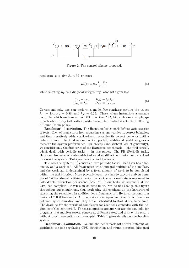
Figure 2: The control scheme proposed.

regulators is to give Rr a PI structure:

Rr(z) = krrz − zrrz − 1

(5)

while selecting Rp as a diagonal integral regulator with gain kpi:

ARp = IN , BRp = kpiIN ,CRp = IN , DRP

= 0N×N .(6)

Correspondingly, one can perform a model-free synthesis getting the valueskrr = 1.4, zrr = 0.88, and kpi = 0.25. These values instantiate a cascadecontroller which we take as our BCC. For the PSC, let us choose a simple ap-proach where every task with a positive computed budget is activated followinga Round Robin policy.

Benchmark description. The Hartstone benchmark defines various seriesof tests. Each of them starts from a baseline system, verifies its correct behavior,and then iteratively adds workload and re-verifies its correct behavior until afailure occurs. The final amount of (supported) additional workload gives ameasure the system performance. For brevity (and without loss of generality),we consider only the first series of the Hartstone benchmark — the “PH series”,which deals with periodic tasks — in this paper. The PH (Periodic tasks,Harmonic frequencies) series adds tasks and modifies their period and workloadto stress the system. Tasks are periodic and harmonic.

The baseline system [18] consists of five periodic tasks. Each task has a fre-quency and a workload. All frequencies are an integral multiple of the smallest,and the workload is determined by a fixed amount of work to be completedwithin the task’s period. More precisely, each task has to execute a given num-ber of “Wheatstones” within a period, hence the workload rate is measured inKilo-Whets instruction per second [KWIPS]. In our tests, we assume that theCPU can complete 1 KWIPS in 25 time units. We do not change this figurethroughout our simulations, thus neglecting the overhead on the hardware ofexecuting the scheduler. In addition, let a frequency of 1 Hertz correspond to aperiod of 20000 time units. All the tasks are independent: their execution doesnot need synchronization and they are all scheduled to start at the same time.The deadline for the workload completion for each task coincides with the be-ginning of the next period. These assumptions are appropriate, for example, forprograms that monitor several sensors at different rates, and display the resultswithout user intervention or interrupts. Table 1 gives details on the baselinesystem.

Benchmark evaluation. We run the benchmark with three different al-gorithms: the one regulating CPU distribution and round duration (designed

10

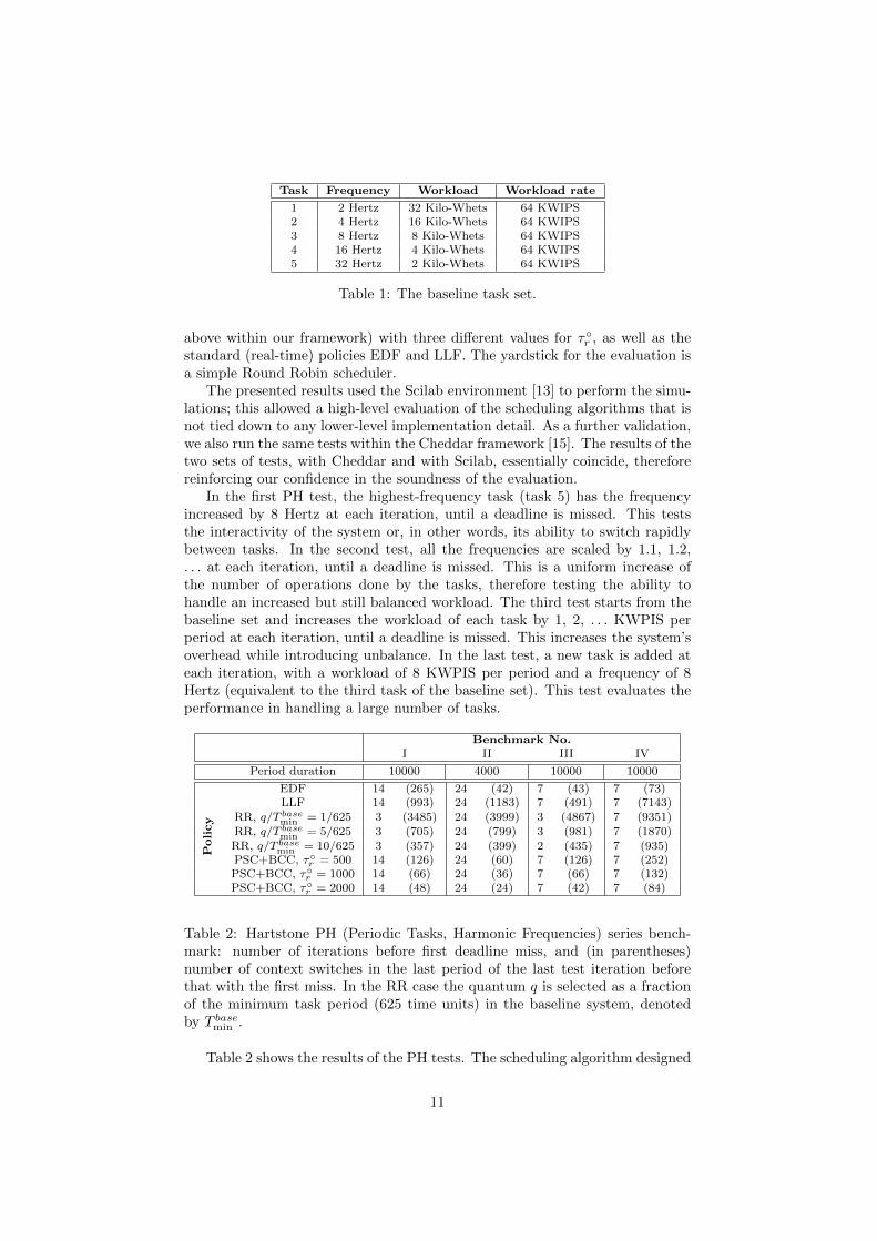
Task Frequency Workload Workload rate

1 2 Hertz 32 Kilo-Whets 64 KWIPS2 4 Hertz 16 Kilo-Whets 64 KWIPS3 8 Hertz 8 Kilo-Whets 64 KWIPS4 16 Hertz 4 Kilo-Whets 64 KWIPS5 32 Hertz 2 Kilo-Whets 64 KWIPS

Table 1: The baseline task set.

above within our framework) with three different values for τ◦r , as well as thestandard (real-time) policies EDF and LLF. The yardstick for the evaluation isa simple Round Robin scheduler.

The presented results used the Scilab environment [13] to perform the simu-lations; this allowed a high-level evaluation of the scheduling algorithms that isnot tied down to any lower-level implementation detail. As a further validation,we also run the same tests within the Cheddar framework [15]. The results of thetwo sets of tests, with Cheddar and with Scilab, essentially coincide, thereforereinforcing our confidence in the soundness of the evaluation.

In the first PH test, the highest-frequency task (task 5) has the frequencyincreased by 8 Hertz at each iteration, until a deadline is missed. This teststhe interactivity of the system or, in other words, its ability to switch rapidlybetween tasks. In the second test, all the frequencies are scaled by 1.1, 1.2,. . . at each iteration, until a deadline is missed. This is a uniform increase ofthe number of operations done by the tasks, therefore testing the ability tohandle an increased but still balanced workload. The third test starts from thebaseline set and increases the workload of each task by 1, 2, . . . KWPIS perperiod at each iteration, until a deadline is missed. This increases the system’soverhead while introducing unbalance. In the last test, a new task is added ateach iteration, with a workload of 8 KWPIS per period and a frequency of 8Hertz (equivalent to the third task of the baseline set). This test evaluates theperformance in handling a large number of tasks.

Benchmark No.I II III IV

Period duration 10000 4000 10000 10000

Policy

EDF 14 (265) 24 (42) 7 (43) 7 (73)LLF 14 (993) 24 (1183) 7 (491) 7 (7143)

RR, q/T basemin = 1/625 3 (3485) 24 (3999) 3 (4867) 7 (9351)

RR, q/T basemin = 5/625 3 (705) 24 (799) 3 (981) 7 (1870)

RR, q/T basemin = 10/625 3 (357) 24 (399) 2 (435) 7 (935)

PSC+BCC, τ◦r = 500 14 (126) 24 (60) 7 (126) 7 (252)PSC+BCC, τ◦r = 1000 14 (66) 24 (36) 7 (66) 7 (132)PSC+BCC, τ◦r = 2000 14 (48) 24 (24) 7 (42) 7 (84)

Table 2: Hartstone PH (Periodic Tasks, Harmonic Frequencies) series bench-mark: number of iterations before first deadline miss, and (in parentheses)number of context switches in the last period of the last test iteration beforethat with the first miss. In the RR case the quantum q is selected as a fractionof the minimum task period (625 time units) in the baseline system, denotedby T basemin .

Table 2 shows the results of the PH tests. The scheduling algorithm designed

11

within our framework shows consistently good performances, and can outper-form other standard algorithms in certain operational conditions for aspectssuch as deadline misses.

Complexity evaluation. Let σPOL denote the time spent during oneround in running the scheduler POL. In our experiments, POL is one of RR,SRR (Selfish Round Robin3), and PSC +BCC.

σRR = N · t→ +N · tc,σSRR = N · t→ +N · tc +N2 · (tS + tΠ) ,

σPSC+BCC = N · t→ +N · tc + (N + 1) · ts+(2N + 1) · tΣ + (2N + 2) · tΠ

(7)

The expressions above take into account the arithmetic operations neces-sary to execute the controller’s code. Then, if we denote the quantum (whereapplicable) by q, the total duration of one round is given by

τr,RR = N · q, τr,SRR = Nw · q, τr,PSC+BCC = τ◦r (8)

where Nw ≤ N is the number of tasks in the waiting queue in the SRR case.Correspondingly, the overall time complexity of the algorithms can be com-

puted. With PSC, it is independent of the number of tasks and can be tunedby changing the round duration parameter. In addition, it is interesting tocompare the complexity of our PSC + BCC algorithm against the RR algo-rithm (an open-loop policy) and the SRR algorithm (a closed-loop variant ofRR, where the possibility of moving tasks between queues provides the feedbackmechanism). It turns out that our PSC + BCC algorithm is computationallyslightly more complex than RR; however, the more complex properties thatPSC + BCC can guarantee — such as convergence to the desired distributionin the presence of disturbances — pay off the additional cost. SRR, on the otherhand, can enforce similar properties and has a greater computational complex-ity than PSC + BCC. The comparison with SRR requires, however, furtherinvestigation, because the parameters of SRR do not seem to have an entirelyclear interpretation within the control-theoretical framework.

5 Conclusion and future work

We presented a framework, based on control theory, to approach the schedulingproblem. The approach clearly separates the models of the processor and ofthe scheduler. This enables the re-use of a vast repertoire of control-theoreticaltechniques to design a scheduling algorithm that achieves certain requirements.Algorithm design is then essentially reduced to controller synthesis. We showedhow to compare the resulting algorithms to existing ones, and the advantagesthat are peculiar to our approach.

This paper focused on developing the components responsible for the com-putation of budgets and the selection of tasks. Future work will focus on thedesign of the intervention policies. This aspect can still be approached withinthe same framework, by analyzing the effects of different policies on the modelequations and on the overall system performance. Moreover, we plan to refinethe complexity evaluation of scheduling algorithms.

3Notice that the SRR is a useful example as it provides an adaptation mechanism.

12

References

[1] L. Abeni, L. Palopoli, G. Lipari, and J. Walpole. Analysis of a reservation-based feedback scheduler. In 23rd IEEE Real-Time Systems Symposium,pages 71–80, 2002.

[2] A. Block, B. Brandenburg, J. Anderson, and S. Quint. Adaptive multi-processor real-time scheduling with feedback control. In 20th EuromicroConference on Real-time Systems, pages 23–33, 2008.

[3] J. Doyle. Robust and optimal control. In 35th IEEE Conf. on Decisionand Control, volume 2, pages 1595–1598, 1996.

[4] J. Hellerstein, Y. Diao, S. Parekh, and D.M. Tilbury. Feedback Control ofComputing Systems. Wiley, 2004.

[5] J.L. Hellerstein, Y. Diao, S. Parekh, and D.M. Tilbury. Control engineeringfor computing systems, industry experience and research challenges. IEEEControl Systems Magazine, 25(6):56–68, 2005.

[6] J. Kay and P. Lauder. A fair share scheduler. Comm. ACM, 31(1):44–55,1988.

[7] D.A. Lawrence, G. Jianwei, S. Mehta, and L.R. Welch. Adaptive schedulingvia feedback control for dynamic real-time systems. In IEEE InternationalConference on Performance, Computing, and Communications, pages 373–378, 2001.

[8] C.L. Liu and J. Layland. Scheduling algorithms for multiprogramming ina hard-real-time environment. Jour. ACM, 20(1):46–61, 1973.

[9] C. Lu, T.F. Abdelzaber, J.A. Stankovic, and S.H. Son. A feedback controlapproach for guaranteeing relative delays in web servers. In 7th Real-TimeTechnology and Applications Symposium, pages 51–62, 2001.

[10] C. Lu, Y. Lu, T.F. Abdelzaher, J.A. Stankovic, and S.H. Son. Feedbackcontrol architecture and design methodology for service delay guaranteesin web servers. IEEE Transactions on Parallel and Distributed Systems,17(9):1014–1027, 2006.

[11] C. Lu, J.A. Stankovic, and S.H. Son. Feedback control real-time schedul-ing: Framework, modeling and algorithms. Journal of Real-Time Systems,23:85–126, 2002.

[12] L. Palopoli and Luca Abeni. Legacy real-time applications in a reservation-based system. IEEE Trans. on Indus. Info., 2009. To appear.

[13] http://www.scilab.org.

[14] L. Sha, T. Abdelzaher, K.E. Arzen, A. Cervin, T. Baker, A. Burns, G. But-tazzo, M. Caccamo, J. Lehoczky, and A.K. Mok. Real time scheduling the-ory: A historical perspective. Real-Time Systems, 28(2-3):101–155, 2004.

[15] F. Singhoff, A. Plantec, P. Dissaux, and J. Legrand. Investigating theusability of real-time scheduling theory with the cheddar project. Journalof Real Time Systems, 43(3):259–295, 2009.

13

[16] A.S. Tanenbaum. Modern Operating Systems. Prentice Hall Press, 2007.

[17] N. Weiderman. Hartstone: Synthetic benchmark requirements for hardreal-time applications. Technical report, CMUSEI-89-TR-23, 1989.

[18] N.H. Weiderman and N.I. Kamenoff. Hartstone uniprocessor bench-mark: definitions and experiments for real-time systems. Real-Time Syst.,4(4):353–382, 1992.

[19] F. Xia and Y. Sun. Control-scheduling codesign: A perspective on inte-grating control and computing. Dynamics of Continuous, Discrete andImpulsive Systems, 13(1):1352–1358, 2006.

14