Embed Size (px)
Citation preview
Knowledge-Based Systems 153 (2018) 65–77
Contents lists available at ScienceDirect
Knowle dge-Base d Systems
journal homepage: www.elsevier.com/locate/knosys
A continuous interval-valued linguistic ORESTE method for
multi-criteria group decision making
Huchang Liao
a , b , Xingli Wu
a , Xuedong Liang
a , ∗, Jian-Bo Yang
c , Dong-Ling Xu
c , Francisco Herrera
b , d
a Business School, Sichuan University, Chengdu 610064, China b Department of Computer Science and Artificial Intelligence, University of Granada, E-18071 Granada, Spain c Manchester Business School, University of Manchester, M15 6PB Manchester, UK d Faculty of Computing and Information Technology, King Abdulaziz University, Jeddah, Saudi Arabia
a r t i c l e i n f o
Article history:
Received 30 September 2017
Revised 14 March 2018
Accepted 19 April 2018
Available online 22 April 2018
Keywords:
Multi-criteria group decision making
Continuous interval-valued linguistic term
set
Extended Gaussian distribution-based
weighting method
ORESTE
Mobike design
a b s t r a c t
Considering that the uncertain linguistic variable (or interval linguistic term) has some limitations in cal-
culation, we extend it to the continuous interval-valued linguistic term set (CIVLTS), which is equivalent
to the virtual term set but has its own semantics. It has the advantages of both the uncertain linguistic
variable and the virtual term set but overcomes their defenses. It not only can interpret more complex
assessments by continuous terms, but also is effective in aggregating the group opinions. We propose
some methods to aggregate the individual decision matrices represented by CIVLTSs to the collective ma-
trix. The extended Gaussian distribution-based weighting method is proposed to derive the weights for
aggregating the large group opinions. Furthermore, the general ranking method ORESTE, is extended to
the CIVL environment and is named as the CIVL-ORESTE method. The proposed method is excellent by
no requirements of crisp criterion weights and the objective thresholds. A case study of selecting the op-
timal innovative sharing bike design for the "Mobike" sharing bikes is operated to show the practicability
of the CIVL-ORESTE method. Finally, we compare the CIVL-ORESTE method with other ranking methods
to illustrate the reliability of our method and its advantages.
© 2018 Published by Elsevier B.V.
1
t
q
o
u
r
d
b
e
v
e
g
g
g
l
p
[
n
m
o
v
t
l
v
t
t
f
t
t
i
g
t
a
h
0
. Introduction
Due to the uncertainty and complexity of objective factors, mul-
iple criteria are defined under qualitative environment, such as
uality, personality and exterior [1–4] . In addition, due to the limit
f knowledge and cognition of single person, a group of individ-
als are invited to make judgments on alternatives to obtain the
eliable evaluation information. Therefore, the multi-criteria group
ecision making (MCGDM) under qualitative context turns out to
e a valuable research issue. This paper focuses on proposing an
ffective method to solve this problem, whose procedures are di-
ided into three parts: expressing the evaluation information of
ach decision-maker (DM), aggregating the DMs’ evaluations to
roup opinions, and ranking the alternatives.
In practice, the opinions of DMs are usually expressed in lin-
uistic terms [5] , which are similar to natural or artificial lan-
uage and close to human’s cognitive process. To avoid information
oss in computational process, some enhanced models were pro-
∗ Corresponding author.
E-mail address: [email protected] (X. Liang).
h
j
w
ttps://doi.org/10.1016/j.knosys.2018.04.022
950-7051/© 2018 Published by Elsevier B.V.
osed, such as the 2-tuple fuzzy linguistic representation model
6] and the virtual linguistic model [7] . These two models are fi-
ally proved to be mathematically equivalent [8] . Given that these
odels are both based on singleton linguistic term while human’s
pinions are always within an interval due to the uncertainty and
agueness in practice, Xu [7] proposed the concept of the uncer-
ain linguistic variable whose value is expressed as the interval of
inguistic terms, such as “between good and very good ”. The interval
ersion of 2-tuple linguistic representation model was also inves-
igated by many scholars [9] . However, people sometimes incline
o express their opinions in natural language with more complex
orm, such as “at least good ”, “more than high ”, but both of the ex-
ended models are unable to represent these pieces of informa-
ion. To solve this problem, Rodríguez et al. [10] proposed the hes-
tant fuzzy linguistic term set (HFLTS) whose value is a set of lin-
uistic terms and the envelope of a HFLTS is an uncertain linguis-
ic variable. Although the HFLTS can represent much information
nd has been proved to be useful in application [11–17] , it also
as some flaws. When people have deep understanding of an ob-
ect, they may provide relatively accurate evaluations. For example,
hen evaluating the satisfaction degree of a product, the expert

66 H. Liao et al. / Knowledge-Based Systems 153 (2018) 65–77
S
s
t
S
n
2
c
m
2
[
D
(
s
s
R
i
t
{
c
e
t
i
d
fi
L
D
{
m
H
a
h
may think it is “between a little high and high and closes to high
with 60% of the proportion ”. The discrete linguistic terms employed
in the existed models are limited to interpret the opinion “closes
to high with 60% of the proportion ”. Using the continuous linguis-
tic term can express this complex information and describe DMs’
views more accurately than the discrete form. Thus, we extend the
uncertain linguistic variable and the HFLTSs into the continuous
interval-valued linguistic term set (CIVLTS) and present the syntax
and semantics.
Integrating individual opinions to collective opinion is an essen-
tial step in MCGDM. Under the linguistic environment, some liter-
atures suggested the union-based methods to aggregate the DMs’
opinions simply [10,17,18] . Given that the probability of each lin-
guistic term is ignored in these union-based methods, Wu and Liao
[19] proposed a group aggregation method by considering both the
expert weights and the probability of the linguistic term. How-
ever, their method is not very effective to aggregate large number
of experts’ opinions which are expressed in continuous linguistic
terms. How to determine each evaluators’ weight is a challenge.
The weights for group members can be intrinsically determined
using their own subjective opinion values. It is appropriate to sup-
pose that the evaluations of a large group obey Gaussian distribu-
tion [20] . In this sense, we can determine DMs’ weights based on
Gaussian distribution. Low weights are given to the “false” or “bi-
ased” judgments while high weights are assigned to the mid eval-
uations, which conform to people’s perceptions.
Ranking alternatives is a critical process to solve the MCGDM
problems. There are mainly two types of ranking methods: the
utility values-based methods and the outranking methods [8] . The
former ranks the alternatives by aggregating the values of each
alternative with respect to all criteria, such as the TOPSIS (Tech-
nique for Order Preference by Similarity to Ideal Solution) [21] and
the VIKOR (VlseKriterijumska Optimizacija I Kompromisno Resenje)
method [18,22] . The obtained results with this type of methods
are clear and intuitive but unable to reflect the incomparability
relation between two alternatives. The latter is based on pair-
wise comparisons, such as the ELECTRE (ELimination Et Choix
Traduisant la REalité - ELimination and Choice Expressing the Real-
ity) method [23] and the Preference Ranking Organization METHod
for Enrichment Evaluations (PROMETHEE) [12,24] . It can determine
the preference (P), indifference (I) and incomparability (R) relations
between alternatives. However, the thresholds to distinguish the
PIR relations are given by DMs subjectively, which makes the re-
sults bad robustness. The ORESTE (organísation, rangement et Syn-
thèse de données relarionnelles, in French) method [25] , is an inte-
grated ranking method which is composed by two stages. It firstly
calculates the utility values to determine weak ranking of alterna-
tives, and then derives the PIR relations by the conflict analysis.
Thus, it shows the advantages of both types of ranking methods
and the thresholds are calculated objectively with less subjective
factors. Furthermore, it does not require the crisp weights of crite-
ria which are sometimes difficult or impossible to determine in lin-
guistic environment but are indispensable in most ranking meth-
ods. However, the tedious process in the classical ORESTE method
leads to information loss to some extent, and it is limited to handle
the evaluations expressed in CIVLTSs.
The aim of this paper to handle the MCGDM problems in which
the CIVLTSs are used to express individuals’ hesitant and qualita-
tive evaluations on alternatives and criteria importance. The aggre-
gation methods including the extended Gauss-distribution-based
weighting method (EGDBWM) is introduced to aggregate the in-
dividuals’ continuous interval-valued linguistic elements (CIVLEs)
to group opinions. Subsequently, we rank the alternatives by the
proposed the continuous interval-valued linguistic ORESTE (CIVL-
ORESTE) method based on the group opinions. The main contribu-
tions of this paper are as follows:
(1) We propose the CIVLTSs to express individuals’ evaluations
and collective opinions exactly. Based on the transform func-
tion, we introduce the basic operations and the comparison
method of the CIVLTSs. They can overcome the defects of
the operations of uncertain linguistic variables that are cal-
culated based on the labels of linguistic terms.
(2) We divide the expert group into four types considering that
different groups are suitable for different aggregation meth-
ods. The union-based method is proposed to derive the
collective opinions of small size group; the average arith-
metic aggregation formula-based method is used to solve
the medium size group, the weighted arithmetic aggrega-
tion formula-based method is used to solve the medium size
group and the EGDBWM is developed to deal with the large
size group.
(3) We improve the ORESTE method by introducing the distance
measure between the CIVLTSs, and derive the thresholds of
the ORESTE within the context of CIVLTSs. We develop the
procedure of the CIVL-ORESTE method.
(4) We provide a helpful reference for the enterprises to select
the optimal innovative sharing bike design and maximize
customer satisfaction based on a case study with the CIVL-
ORESTE method.
The remainder of this paper is structured as follows.
ection 2 introduces the CIVLTS and its semantics. Section 3 de-
cribes some methods to aggregate individual decision matrices
o collective matrix. Section 4 proposes the CIVL-ORESTE method.
ection 5 introduces a case study about selecting the optimal in-
ovative sharing bike design. Section 6 presents some conclusions.
. Continuous interval-valued linguistic term set
This section introduces a general representation form of the un-
ertain linguistic variable, i.e., the CIVLTS, and then justifies its se-
antics in describing linguistic information.
.1. Uncertain linguistic variable and HFLTS
To preserve more information than one linguistic term, Xu
7] introduced the concept of uncertain linguistic variable.
efinition 1 [7] . Let S ′ = { s 0 , s 1 , ..., s τ } be a linguistic term set
LTS). s = [ s α, s β ] is an uncertain linguistic variable, where s α ,
β ∈ S ′ , and s α and s β are the lower and the upper limits of s , re-
pectively.
emark 1. The subscripts of the linguistic terms s α and s β are
ntegers. To avoid information loss in calculation, Xu [7] ex-
ended the discrete term set S ′ to a continuous term set S = s α| s 0 ≤ s α ≤ s τ , α ∈ [0 , τ ] } and called it as the virtual term set. It
an only appear in calculation while the original LTS is used in
valuation.
The uncertain linguistic variable can only be used to represent
he linguistic expressions in the form of “between s k and s m
”, but
ndividuals always have much richer expressions. In this sense, Ro-
ríguez et al. [10] introduced the concept of HFLTSs as an ordered
nite subset of the consecutive linguistic terms of S ′ . Afterwards,
iao et al. [11] extended and formalized the HFLTS mathematically.
efinition 2 [11] . Let x i ∈ X ( i = 1 , 2 , . . . , N ) be fixed and S = s t | t = −τ, . . . , −1 , 0 , 1 , . . . , τ} be a LTS. A HFLTS on X, H S , is in
athematical form of
S = { < x i , h S ( x i ) > | x i ∈ X } where h S ( x i ) is a set of some values in S and can be expressed
s
S ( x i ) = { s ϕ ( x i ) | s ϕ ( x i ) ∈ S, l = 1 , . . . , # h S ( x i ) }
l l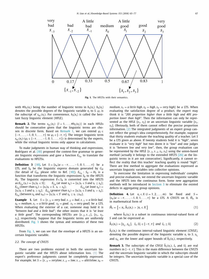
H. Liao et al. / Knowledge-Based Systems 153 (2018) 65–77 67
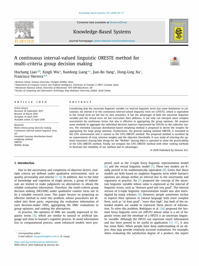
Fig. 1. The HFLTSs with their semantics.
w
d
t
t
R
s
s
{
s
w
R
a
e
D
L
(
f
H
a
E
{
E
E
s
W
“
a
s
d
H
c
2
g
e
F
m
e
t
p
s
s
i
n
t
b
e
i
b
m
g
fl
T
u
a
a
m
d
D
{
i
H
S
h
h
d
a
R
n
a
b
C
ith # h S ( x i ) being the number of linguistic terms in h S ( x i ). h S ( x i )
enotes the possible degrees of the linguistic variable x i to S . ϕl is
he subscript of s ϕ l ( x i ) . For convenience, h S ( x i ) is called the hesi-
ant fuzzy linguistic element (HFLE).
emark 2. The terms s ϕ l ( x i ) ( l = 1 , . . . , # h S ( x i ) ) in each HFLEs
hould be consecutive given that the linguistic terms are cho-
en in discrete form. Based on Remark 1 , we can extend ϕ l ∈−τ, . . . , −1 , 0 , 1 , . . . , τ } to ϕ l ∈ [ −τ, τ ] . The integer linguistic term
ϕ l ( x i ) ( ϕ l ∈ {−τ, . . . , −1 , 0 , 1 , . . . , τ } ) is determined by the experts,
hile the virtual linguistic terms only appear in calculations.
To make judgments in human way of thinking and expressions,
odríguez et al. [10] proposed the context-free grammar to gener-
te linguistic expressions and gave a function E G H to translate the
valuations to HFLTSs.
efinition 3 [10] . Let S = { s α| α = −τ, . . . , −1 , 0 , 1 , . . . , τ} be a
TS, and S ll be the linguistic express domain generated by G H
for detail of G H , please refer to Ref. [10] ). E G H : S ll → H S is a
unction that transforms the linguistic expressions S ll to the HFLTS
S . The linguistic expression ll ∈ S ll is converted into the HFLTS
s: E G H ( s t ) = { s t | s t ∈ S } ; E G H (at most s k ) = { s t | s t ∈ S and s t ≤ s k } ; G H
(lower than s k ) = { s t | s t ∈ S, s t < s k } ; E G H (at least s k ) = s t | s t ∈ S and s t ≥ s k } ; E G H ( greater than s k ) = { s t | s t ∈ S and s t > s k } ; G H
( between s k and s m
) = { s t | s t ∈ S ′ and s k ≤ s t ≤s m
} . xample 1. Let S = { s −3 = v ery bad, s −2 = bad, s −1 = a lit t le bad,
0 = medium, s 1 = a lit t le good, s 2 = good, s 3 = v ery good} be a LTS.
hen evaluating the exterior of a car, someone may hold it is
between bad and a little bad”; the other insists that it is “at least
little good”. The corresponding HFLTEs are { s −2 , s −1 } , { s 1 , s 2 ,
3 }, respectively. Suppose that the linguistic terms are uniformly
istributed. Fig. 1 shows the syntax and semantics of these two
FLTEs.
From Fig. 1 , we can see that the envelope of a HFLTS is an un-
ertain linguistic variable.
.2. The concept of CIVLTS
There are two problems existed in both the uncertain lin-
uistic variable and the HFLTS about information loss. (1) The
xpert’s preference judgments cannot be completely expressed.
or example, let S = { s −3 = v erylow, s −2 = low, s −1 = alit t lelow, s 0 =
edium, s 1 = a lit t le high, s 2 = high, s 3 = v ery high } be a LTS. When
valuating the satisfaction degree of a product, the expert may
hink it is “20% proportion higher than a little high and 40% pro-
ortion lower than high ”. Then the information can only be repre-
ented as the HFLE { s 1 , s 2 } or an uncertain linguistic variable [ s 1 ,
2 ]. Obviously, both of them cannot reflect the precise proportion
nformation. (2) The integrated judgments of an expert group can-
ot reflect the group’s idea comprehensively. For example, suppose
hat thirty students evaluate the teaching quality of a teacher. Let S
e a LTS given as above. If twenty students hold it is “high ”, seven
valuate it is “very high ” but two deem it is “low ” and one judges
t is “between low and very low ”, then, the group evaluation can
e represented by the HFLE { s −3 , s −2 , s 2 , s 3 } using the union-based
ethod (actually it belongs to the extended HFLTS [26] as the lin-
uistic terms in it are not consecutive). Significantly, it cannot re-
ect the reality that this teacher’ teaching quality is round “high ”.
here are few method to aggregate the evaluations expressed as
ncertain linguistic variables into collective opinions.
To overcome the limitation in expressing individuals’ complex
nd precise evaluations, we extend the uncertain linguistic variable
nd the HFLTS into the continuous form. Some new aggregation
ethods will be introduced in Section 3 to eliminate the existed
efects in aggregating group opinions.
efinition 4. Let x i ∈ X ( i = 1 , 2 , . . . , m ) be fixed and S = s α| α = −τ, . . . , −1 , 0 , 1 , . . . , τ} be a LTS. A CIVLTS on X , ˜ H S , is
n mathematical form of
˜ S =
{< x i , h S ( x i ) > | x i ∈ X
}(1)
where ˜ h S ( x i ) is a subset in continuous internal-valued form of
and can be expressed as
˜ S ( x i ) = [ s L i , s U i ] , L i , U i ∈ [ −τ, τ ] and L i ≤ U i (2)
˜ S ( x i ) is the continuous interval-valued linguistic element (CIVLE),
enoting the possible degrees of the linguistic variable x i to S . s L i nd s U i are the lower and upper bounds of ˜ h S ( x i ) , respectively.
emark 3. The subscripts of the CIVLE ˜ h S ( x i ) , L i and U i are real
umbers in [ −τ, τ ] . This is the main difference between the CIVLTS
nd the uncertain linguistic variable in which the subscripts should
e integers. The uncertain linguistic variable is a special case of the
IVLTS.

68 H. Liao et al. / Knowledge-Based Systems 153 (2018) 65–77
Fig. 2. The syntax and semantic of the CIVLE h 3 S .
(
g
w
b
g
w
E
D
h
E
h
h
g
[
E
i
As we can see, the CIVLTS is mathematical equivalent to the
interval-valued virtual term set. However, the interval-valued vir-
tual term set cannot be used to represent the evaluators’ assess-
ments. The main contribution of the CIVLTS is that it has its own
semantics and thus overcomes the defense of the interval-valued
virtual term set. The CIVLTS can be used to represent the evalua-
tors’ judgments directly. This can be justified by Example 2 .
Example 2. Suppose that someone evaluates the complexity
of a certain procedure. Let S = { s −3 = extremely complex, s −2 =v ery complex, s −1 = complex, s 0 = medium, s 1 = easy, s 2 = v ery easy,
s 3 = extremly easy } be a LTS. If one is uncertain, he/she can say
it is “complex ” ( h 1 S ) or “between medium and complex ” ( h 2
S ). If one
can make a more accurate judgment, he/she can say it is “between
medium and complex but closes to complex ” ( h 3 S ). If one can make
an extremely accurate judgment, he/she can say it is “between
medium and complex but 80% proportion closes to complex ” ( h 4 S ).
Then the corresponding CIVLEs are ˜ h 1 S = [ s −1 , s −1 ] , ˜ h 2 S = [ s −1 , s 0 ] ,
˜ h 3 S
= [ s −1 , s −0 . 5 ] , ˜ h 4 S
= [ s −1 , s −0 . 8 ] , respectively. Suppose that the
linguistic terms are uniformly distributed. Fig. 2 shows the syntax
and semantics of ˜ h 3 S .
It should be noted that the absolute deviation between adjacent
linguistic terms is not always equal. For example, the deviation be-
tween “medium” and “high” may be large than the deviation be-
tween “high” and “very high” in term of the quality of a product.
That is to say, the symbols and semantics of the linguistic terms
are disproportionate under some situations. Thus, it is irrational to
calculate the linguistic terms directly by the their subscripts. Wang
et al. [13] proposed some transformation functions to translate the
linguistic term into its semantic.
Let s t , t ∈ [ −τ, τ ] be a linguistic term, and ϕt be a numeric
value which denotes the semantic of s t . The transformation func-
tion between s t and ϕt is defined as: g: s t → ϕt ; g −1 : ϕt → s t ( t ∈[ −τ, τ ] ). Based on Ref. [13] , (1) if the absolute deviations between
adjacent linguistic terms are equal, then
g( s t ) = (τ + t) / 2 τ (3)
2) if they increases with the extension from s 0 , then
( s t ) =
⎧ ⎪ ⎨
⎪ ⎩
ρτ − ρ−t
2 ρτ − 2
, if t ∈ [ −τ, 0]
ρτ + ρt − 2
2 ρτ − 2
, if t ∈ (0 , τ ]
(4)
here ρ =
τ√
d and d is the deviation between s 0 and s τ which can
e determined according to the actual situation.
( 3 ) if they decreases with the extension from s 0 , then
( s t ) =
⎧ ⎪ ⎨
⎪ ⎩
τλ − (−t) λ
2 τλ, if t ∈ [ −τ, 0]
τ γ + (t) γ
2 τλ, if t ∈ (0 , τ ]
(5)
here λ, γ ∈ (0, 1] can be determined based on the practical case.
specially, if λ, γ = 1 , then g( s t ) = (τ + t) / 2 τ .
efinition 6. Let S = { s α| α = −τ, . . . , −1 , 0 , 1 , . . . , τ} be a LTS, and˜ S = [ s L , s U ] , ˜ h 1
S = [ s L 1 , s U 1 ] ,
˜ h 2 S
= [ s L 2 , s U 2 ] be three CIVLEs, then
(1) Union: ˜ h 1 S
∪
h 2 S
= [ min { s L 1
, s L 2
} , max { s U 1
, s U 2
} ] ; (2) Intersection: ˜ h 1 S ∩
h 2 S = [ max { s L 1 , s L 2 } , min { s U 1 , s U 2 } ] ; if
max { s L 1
, s L 2
} > min { s U 1
, s U 2
} , then
˜ h 1 S
∩
h 2 S = φ;
(3) Complement: ˜ h C S
= [ s −τ , s L ] ∪ [ s U , s τ ] ;
(4) ˜ h 1 S �˜ h 2 S = [ s L 1
, s U 1 ] � [ s L 2
, s U 2 ] = [ g −1 (g( s L 1 ) +
g( s L 2 )) , g −1 (g( s U 1 ) + g( s U 2 ))] ;
(5) λ˜ h S = λ[ s L , s U ] = [ g −1 (λg( s L )) , g −1 (λg( s U ))] , where λ∈ [0, 1];
(6) ( h S ) λ = [ g −1 (g ( s L )
λ) , g −1 (g ( s U ) λ)] , where λ∈ [0, 1].
xample 3. Let S = { s −3 , · · · , s 0 , · · · , s 3 } be a LTS, ˜ h S = [ s 1 . 2 , s 1 . 8 ] ,˜
5 S
= [ s −1 , s 0 ] , ˜ h 6 S
= [ s 0 , s 1 ] be three CIVLEs and λ = 0 . 8 . Then
˜ h 5 S
∪˜
6 S
= [ s −1 , s 1 ] ; h 5 S
∩
h 6 S
= [ s 0 , s 0 ] ; ˜ h C S
= [ s −3 , s 1 . 2 ] ∪ [ s 1 . 8 , s 3 ] ; if g ( s t ) is
iven as Eq. (4) and ρ = 2 , then λ˜ h 5 S
� (1 − λ) h 6 S
= [ s −0 . 85 , s 0 . 26 ] ;
( h S ) λ = [ s 1 . 69 , s 2 . 09 ] .
To compare the CIVLEs, we define the expect function of ˜ h S = s L , s U ] based on the transformation function as:
( h S ) =
1
2
(g( s L ) + g( s U )) (6)
If E( h 1 S ) > E( h 2
S ) , then
˜ h 1 S
� ˜ h 2 S ; if E( h 1
S ) < E( h 2
S ) , then
˜ h 1 S
≺ ˜ h 2 S ;
f E ( h 1 S ) = E ( h 2
S ) , we further define the variance function to make

H. Liao et al. / Knowledge-Based Systems 153 (2018) 65–77 69
c
D
D
E
h
a
0
3
c
3
t
a
o
r
Q
i
D
[
t
q
d
e
[
l
a
s
t
h
3
g
g
e
b
d
t
j
[
f
v
o
s
t
t
l
v
u
p
t
l
s
p
t
r
w
omparison as:
( h S ) =
√ (g( s L ) −E( h S )
)2 +
(g( s U ) −E( h S )
)2 (7)
When E ( h 1 S ) = E ( h 2
S ) , if D ( h 1
S ) < D ( h 2
S ) , then
˜ h 1 S
� ˜ h 2 S ; if D ( h 1
S ) >
( h 2 S ) , then
˜ h 1 S ≺ ˜ h 2 S ; if D ( h 1 S ) = D ( h 2 S ) , then
˜ h 1 S ≈ ˜ h 2 S .
xample 4. Let S = { s −3 , · · · , s 0 , · · · , s 3 } be a LTS, and
˜ h 5 S
= [ s −1 , s 0 ] ,
˜
6 S
= [ s 0 , s 1 ] and
˜ h 7 S
= [ s 0 . 5 , s 0 . 5 ] be three CIVLEs. If g ( s t ) is given
s Eq. (5) and λ = 0 . 6 , γ = 0 . 7 , we can get E( h 5 S ) = 0 . 36 , E( h 6
S ) =
. 615 and E( h 7 S ) = 0 . 64 . Thus ˜ h 7
S >
h 5 S
>
h 6 S .
. Methods to aggregate individual decision matrices to
ollective matrix
.1. Description of the MCGDM problem with CIVLEs
A general MCGDM method consists of a finite set of m alterna-
ives A = { a 1 , ..., a i , ..., a m
} , a set of n criteria C = { c 1 , ..., c j , ..., c n } ,nd a set of Q DMs E = { e 1 , ..., e q , ..., e Q } . The DM e q is supposed to
ffer the evaluation value for alternative a i with respect to crite-
ion c j in CIVLE, namely, ˜ h i j(q ) S
= [ s i j(q )
L , s i j(q )
U ] . Then we can construct
judgment matrices D
(q ) = ( h i j(q ) S
) m ×n , q = 1 , ..., Q .
Due to the complexity of the MCGDM problem and the ambigu-
ty of human thoughts as well as the different opinions among the
Ms, in practice, it is hard to assign a crisp weight to each criterion
27] . Generally, the criterion importance degree ranges in fuzzy in-
erval, such as “between importance and very importance”. Conse-
uently, the precise criterion weights, which are given by the DMs
irectly or obtained by some techniques such as the AHP [28] , the
ntropy function [29] and the prioritized operator-based method
30] , may result in information distortion and thus reduce the re-
iability of the final decision results. In this sense, the DM e q is
sked to give the weight of the criterion c j in linguistic expres-
ion, which then can be transformed to the CIVLE ˜ h j(q ) S
. The collec-
ive criterion weight ω j =
h j S
is the aggregation value of the CIVLEs
˜
j(q ) S
( q = 1 , ..., Q) given by the DMs.
.2. Aggregating group opinions with CIVLEs
This subsection proposes some aggregation methods to inte-
rate the individual judgment matrices D
( q ) , q = 1 , ..., Q to the
roup decision matrix D = ( h i j S ) m ×n .
Sometimes we suppose that the DMs have equal weights. How-
ver, in most cases, different DMs should have different weights
ecause their different knowledge and experience may lead to the
iscrepancies in evaluation quality [31] . There are some methods
o determine the weights of the DMs, such as the consistency
udgement method [14] and the cluster analysis based method
15] . These methods are complicated and do not consider the dif-
erent characteristics of the group members. In this section, we di-
ide the MCGDM problems into four types according to the scale
f the group. Different aggregation methods can be used with re-
pect to different types. It should be noted that below we only give
he aggregation methods over the assessments on alternatives, and
he aggregation on the weights of criteria is the same.
(1) Small size group. For a group of less than three members,
as it is easy to compromise with each other, computing the
union is an appropriate method to integrate the DMs’ evalu-
ations, shown as Eq. (8) . If there are few prejudices, we can
delete them.
˜ h
i j S
=
˜ h
i j(1) S
∪ ... ∪
h
i j(q ) S
∪ ... ∪
h
i j(Q ) S
=
[min { s i j(1)
L , ..., s i j(q )
L , ..., s i j(Q )
L } ,
max { s i j(1) U
, ..., s i j(q ) U
, ..., s i j(Q ) U
} ] (8)
(2) Medium size group. For a medium scale group of three to
five members, generally, there may be different opinions but
all maintain referential significance. Thus, we can assign the
same weight to the DMs. The average arithmetic aggregation
formula is shown in Eq. (9) . Note that if there are few prej-
udices, we can reject them; if the disparity of the evaluation
quality is great, we can give different weights to DMs.
˜ h
i j S
= [ s i j L , s i j
U ] =
[
1
Q
Q ∑
q =1
s i j(q ) L
, 1
Q
Q ∑
q =1
s i j(q ) U
]
(9)
(3) Medium to large size group. For a group of six to thirty
members with different knowledge and experience, the
weight of DM e q , w
(q ) , may be assigned in advance. Then the
collective opinion can be calculated by the weighted arith-
metic aggregation operator shown as:
˜ h
i j S
= [ s i j L , s i j
U ] =
[
w
(q ) Q ∑
q =1
s i j(q ) L
, w
(q ) Q ∑
q =1
s i j(q ) U
]
(10)
(4) Large size group. For a large-scale group of more than thirty
members, it is appropriate to suppose that the evaluations
determined by the DMs obey Gaussian distribution given
that most of them hold the similar opinions but a few of
them insist different opinions since the evaluation on an al-
ternative is affected by many small independent random fac-
tors. In this case, assigning the same weight to each DM
is obviously unreasonable. Low weights should be given to
the “false” or “biased” judgments while high weights should
be assigned to the mid evaluations. The probability density
function of Gaussian distribution for a random variable x is
defined as f (x ) =
1 √
2 πσe −[ (x −u ) 2 / 2 σ 2 ] , x ∈ (−∞ , + ∞ ) where
u is the mean value and σ is the standard deviation of x .
The farther x away from u is, the smaller the value of f ( x )
is. Inspired by this property, Xu [ 20 ] used f ( q ) to repre-
sent the weight of each individual where q is the order of
the evaluation value. However, there are some flaws in Xu’s
method: (1) the discrete orders, 1, ���, q , ���, Q , essentially,
are disobeyed to the Gauss distribution; (2) the differences
of the evaluation values were ignored in Xu’s method (which
may lead to an unacceptable result that the same evalu-
ations may get different weights while the different judg-
ments may get the same weight); (3) it is limited to handle
the linguistic evaluations.
To avoid the above flaws, we introduce an EGDBM, which uti-
izes the interval-valued linguistic evaluation value itself as random
alue, to calculate the weight of DM. Then, we can calculate the
pper and lower limits of the group CIVLEs by aggregating the up-
er and lower bounds of the individual CIVLEs, respectively.
Let W L = (w
(1) L
, ..., w
(q ) L
, ..., w
(Q ) L
) T be the weight vec-
or of the lower limits L = (s (1) L
, ..., s (q ) L
, ..., s (Q ) L
) T and W U =(w
(1) U
, ..., w
(q ) U
, ..., w
(Q ) U
) T be the weight vector of the upper
imits U = (s (1) U
, ..., s (q ) U
, ..., s (Q ) U
) T . Based on the probability den-
ity function of Gaussian distribution, we can determine the
robability density value of each lower limit as f (s (q ) L
) =1 √
2 πσe −[ ( L (q ) −u L )
2 / 2 ( σL )
2 ] , f (s (q ) U
) =
1 √
2 πσe −[ ( U (q ) −u U )
2 / 2 ( σU )
2 ] . Af-
er normalization, the weights of the lower and upper limits are
espectively calculated as
(q ) L
=
e −[ ( L (q ) −u L ) 2 / 2 ( σL )
2 ] ∑ Q
q =1 e −[ ( L (q ) −u L )
2 / 2 ( σL )
2 ] ,
70 H. Liao et al. / Knowledge-Based Systems 153 (2018) 65–77
Fig. 3. The Gaussian distribution values of the lower and upper limits derived by the EGDBW method.
4
g
b
i
g
c
r
u
r
[
p
b
D
w
t
r
1
R
s
T
�
t
T
t
o
t
μ
w
a
i
R
w
(q ) U
=
e −[ ( U (q ) −u U ) 2 / 2 ( σU )
2 ] ∑ Q
q =1 e −[ ( U (q ) −u U )
2 / 2 ( σU )
2 ] , q = 1 , ..., Q (11)
where u L and σ L are the mean and variance of the upper limits,
u U and σ U are the mean and variance of the upper limits, and L ( q )
and U
( q ) are the subscripts of s (q ) L
and s (q ) U
, respectively.
Then, we can obtain the group assessments as
˜ h
i j S
=
[s i j
L , s i j
U
]=
[
Q ∑
q =1
w
(q ) L
s i j(q ) L
,
Q ∑
q =1
w
(q ) U
s i j(q ) U
]
(12)
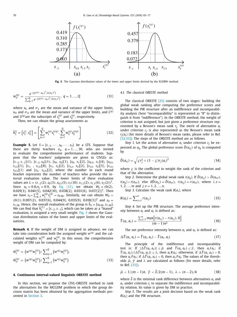
Example 5. Let S = { s −3 , · · · , s 0 , · · · , s 3 } be a LTS. Suppose that
there are thirty teachers e q , q = 1 , ..., 30 , who are invited
to evaluate the comprehensive performance of students. Sup-
pose that the teachers’ judgments are given in CIVLEs as:
[ s −2 , s −1 ](1) , [ s −2 , s 0 ](1) , [ s 0 , s 0 ](1), [ s 0 , s 1 ](2), [ s 0.5 , s 1 ](4), [ s 0.5 ,
s 1.5 ](1), [ s 1 , , s 1.5 ](8), [ s 1 , s 2 ](2), [ s 1.2 , s 2 ](2), [ s 1.5 , s 2 ](5), [ s 1.5 ,
s 2.5 ](1) and [ s 2 , s 2.5 ](2), where the number in each round
bracket represents the number of teachers who provide the in-
terval evaluation value. The lower limits of these evaluation
values are L = ( s −2 (2) , s 0 (3) , s 0 . 5 (5) , s 1 (10) , s 1 . 2 (2) , s 1 . 5 (6) , s 2 (2) ) T .
Since u L = 0 . 8 , σL = 0 . 9 , by Eq. (11) , we obtain W L = (0(2) ,
0.029(3), 0.041(5), 0.042(10), 0.038(2), 0.031(6), 0.017(2)) T . Then
we have s L =
∑ Q q =1
w
(q ) L
s (q ) L
= s 0 . 96 . Similarly, we can obtain W U =(0(1) , 0 . 007(2) , 0.037(6), 0.044(9), 0.035(9), 0.018(3)) T and s U =s 1 . 58 . Hence, the overall evaluation of the group is ˜ h S = [ s 0 . 96 , s 1 . 58 ] .
We can find that ˜ h (1) S
= [ s −2 , s −1 ] , which can be taken as a “biased”
evaluation, is assigned a very small weight. Fig. 3 shows the Gaus-
sian distribution values of the lower and upper limits of the eval-
uations.
Remark 4. If the weight of DM is assigned in advance, we can
take into consideration both the assigned weight w
(q ) and the cal-
culated weights w
(q ) t and w
(q ) k
. In this sense, the comprehensive
weight of DM can be computed by:
˜ w
(q ) L
=
(w
(q ) w
(q ) L
)/ ∑ Q
q =1
(w
(q ) w
(q ) L
),
˜ w
(q ) U
=
(w
(q ) w
(q ) U
)/ ∑ Q
q =1
(w
(q ) w
(q ) U
)(13)
4. Continuous interval-valued linguistic ORESTE method
In this section, we propose the CIVL-ORESTE method to rank
the alternatives for the MCGDM problem in which the group de-
cision matrix has been obtained by the aggregation methods pre-
sented in Section 3 .
.1. The classical ORESTE method
The classical ORESTE [25] consists of two stages: building the
lobal weak ranking after computing the preference scores and
uilding the PIR structure after an indifference and incomparabil-
ty analysis (here “incomparability” is represented as “R ” to distin-
uish it from “indifference”). In the ORESTE method, the weight of
riterion is not assigned, but just given a preference structure rep-
esented by a Besson’s mean rank r j . The merit of alternative a i nder criterion c j is also represented as the Besson’s mean rank
j ( a i ) (for more details of Besson’s mean ranks, please refer to Ref.
32,33] ). The steps of the ORESTE method are as follows.
Step 1. Let the action of alternative a i under criterion c j be ex-
ressed as a ij . The global preference score ˜ D ( a i j ) of a ij is computed
y
˜ ( a i j ) =
√
ς r 2 j + (1 − ς ) r j ( a i )
2 (14)
here ς is the coefficient to weight the rank of the criterion and
hat of the alternative.
Step 2. Determine the global weak rank r ( a ij ). If ˜ D ( a i j ) >
˜ D ( a zv ) ,
( a ij ) > r ( a zv ); else if D ( a i j ) =
˜ D ( a zv ) , r( a i j ) = r( a zv ) , where i, z = , 2 , ..., m and j, v = 1 , 2 , ..., n .
Step 3. Calculate the weak rank R ( a i ), where
( a i ) =
∑ n
j=1 r( a i j ) (15)
Step 4. Set up the PIR structure. The average preference inten-
ity between a i and a z is defined as:
˜ ( a i , a z ) =
∑ n j=1 max
[r( a z j ) − r( a i j ) , 0
](m − 1) n
2 (16)
The net preference intensity between a i and a z is defined as:
˜ T ( a i , a z ) =
˜ T ( a i , a z ) − ˜ T ( a z , a i ) (17)
The principle of the indifference and incomparability
est is: If | � ˜ T ( a i , a z ) | ≤ ˜ μ and
˜ T ( a i , a z ) ≤ ˜ γ , then a i I a z ; if˜ ( a i , a z ) / | � ˜ T ( a i , a z ) | ≥ λ, then a i R a z ; otherwise, if � ˜ T ( a i , a z ) > 0 ,
hen a i P a z ; if � ˜ T ( a i , a z ) < 0 , then a z P a i . The values of the thresh-
lds ˜ μ, ˜ γ and λ are calculated as follows (for more details, refer
o Ref. [33] ).
˜ < 1 / ( m − 1 ) n, ˜ γ <
˜ δ/ 2 ( m − 1 ) , λ > ( n − 2 ) / 4 (18)
here ˜ δ is the minimal rank difference between alternatives a i and
z under criterion c j to separate the indifference and incomparabil-
ty relation. Its value is given by DM in practice.
Step 5. The results are a joint decision based on the weak rank
( a ) and the PIR structure.
i
H. Liao et al. / Knowledge-Based Systems 153 (2018) 65–77 71
O
c
p
s
t
w
b
d
fi
t
t
t
t
i
O
s
4
t
t
r
E
E
b
e
g
g
v
p
h
i
r
l
H
t
T
m
E
d
D
h
d
d
s
c
E
a
d
t
w
h
i
ω
t
r
e
b
t
e
a
t
(
g
j
f
w
Researchers subsequently analyzed the characteristics of the
RESTE method. Bourguignon and Massart [32] analyzed the ne-
essity and significance to distinguish the indifference and incom-
arability relation between alternatives deeply. Pastijn and Ley-
en [33] carried detailed analysis and explanation on the values of
hresholds in the indifference and incomparability analysis frame-
ork. Then a sensitivity analysis for the thresholds was employed
y Delhaye et al. [34] , which indicated that different values have
ifferent influences on results. It has been applied in the various
elds, such as agricultural investment decision [35] , and Radar de-
ection strategy selection [36] , web design firm selection [37] and
he firm performance efficiency order construction [38] .
However, (1) the decision matrix handled by the ORESTE con-
ains less evaluations; (2) translating the global preference scores
o global weak ranks makes information loss; (3) the thresholds ˜ δs hard to determine. To overcome these defects, we improve the
RESTE method, and then combine it with the CIVLTSs in the next
ubsection.
.2. The CIVL-ORESTE method for MCGDM
In this part, the CIVL-ORESTE method is developed to rank
he alternatives according to the collective decision matrix D =( a i j ) m ×n and the weight vector W = ( ω 1 , ..., ω j , ..., ω n ) T of the cri-
eria.
In classical ORESTE, the Besson’s mean ranks r j (1, ..., n ) and
j ( a i ) (i = 1 , ..., m ) would result in information loss seriously.
xample 6 can demonstrate this point.
xample 6. Suppose that three hospitals a 1 , a 2 , a 3 need to
e assessed according to their medical levels and S = { s −3 =xtremely poor, s −2 = v ery poor, s −1 = poor, s 0 = medium, s 1 =
ood, s 2 = v ery good, s 3 = extremly good } is a given LTS. The lin-
uistic evaluations are “a 1 is good ”, “a 2 is between good and
ery good and close to good ” and “a 3 is between poor and very
oor ”, respectively. The corresponding CIVLEs are ˜ h S ( a 1 ) = [ s 1 , s 1 ] ,˜ S ( a 2 ) = [ s 1 , s 1 . 5 ] and
˜ h S ( a 3 ) = [ s −2 , s −1 ] . According to the compar-
son method for CIVLEs given as Eqs. (6 ) and (7) , we can get the
anks r( a 1 ) = 2 , r( a 2 ) = 1 and r( a 3 ) = 3 . Clearly, for the medical
evel, a 1 is extremely close to a 2 but a 3 is far behind a 1 and a 2 .
owever, the ranks reflect the same degree of difference between
he hospitals and thus weaken the information seriously.
Therefore, the ranks in operations are supposed to be replaced.
o maintain the evaluation information completely, the distance
easure is designed to substitute for the ranks. Motivated by the
uclidean distance between HFLEs [17] , we define the Euclidean
istance between CIVLEs as follows.
efinition 7. Let S = { s α| α = −τ, . . . , −1 , 0 , 1 , . . . , τ} be a LTS, and˜
1 S
= [ s 1 L , s 1
U ] and
˜ h 2 S
= [ s 2 L , s 2
U ] be two CIVLEs on S . The Euclidean
istance between
˜ h 1 S
and
˜ h 2 S
is
( h
1 S ,
h
2 S ) =
[
1
2
( | L 1 − L 2 | 2 τ
)2
+
1
2
( | U 1 − U 2 | 2 τ
)2 ] 1 / 2
(19)
Apparently, 0 ≤ d( h 1 S , h 2 S ) ≤ 1 and d( h 1 S ,
h 2 S ) = d( h 2 S , h 1 S ) . The
maller the distance is, the similar of ˜ h 1 S
and
˜ h 2 S
should be. Espe-
ially, if d( h 1 S , h 2
S ) = 0 , then
˜ h 1 S
=
h 2 S .
xample 7. The Euclidean distance between
˜ h S ( a 1 ) , ˜ h
S ( a 2 )
nd
˜ h S ( a 3 ) in Example 6 are: d( h S ( a 1 ) , h S ( a 2 )) = 0 . 0589 ,
( h S ( a 1 ) , h
S ( a 3 )) = 0 . 5 and d( h
S ( a 2 ) , h
S ( a 3 )) = 0 . 4602 . It is clear
hat a 1 is similar to a 2 , and a 3 is highly different from a 1 and a 2 ,
hich is fully in accordance with the reality.
We define the maximum CIVLE of a i under criterion c j as
˜
j+ S
=
{
max i =1 , 2 , ... ,m
{˜ h
i j S
}, for the benefit criterion c j
min
i =1 , 2 , ... ,m
{˜ h
i j S
}, for the cost criterion c j
(20)
Additionally, the weight of the most important criterion c j sat-
sfies
+ = max j=1 ,...,n
ω j = max j=1 ,...,n
{˜ h
j S
}(21)
Let the distance d( h i j S , h
j+ S
) be abbreviated as d ij which is used
o replace r j ( a i ); the distance d( ω j , ω
+ ) be abbreviated as d j to
eplace r j . Then, following the classical ORESTE method, the op-
ration processes of the CIVL-ORESTE are divided into two stages
ased on d ij and d j .
Stage 1. Construct a weak ranking
(1) Compute the global preference score D ( a ij ). Let the coordi-
nate of the action a ij be represented as ( d ij , d j ); let the global
optimal point a + i j+ at coordinate origin be the best alterna-
tive under the most important criteria. Then, we introduce
the weighted Euclidean distance between a ij and a + i j+ as the
global preference score D ( a ij ) of a ij :
D ( a i j ) = d( a i j , a + i j+ ) =
[ξ ( d i j )
2 + (1 − ξ ) ( d j ) 2 ]1 / 2
(22)
where ξ ∈ [0, 1] denotes the relative importance between
d ij and d j .This paper deems d ij and d j are equally impor-
tant, and ξ = 0 . 5 . Like the Euclidean distance between two
CIVLEs, D ( a ij ) ∈ [0, 1], and the smaller it is, the better a ij should be.
(2) Compute the preference score D ( a i ). The preference score of
alternative a i is defined as the average of the global prefer-
ence score of a i j (i = 1 , ..., m ) :
D ( a i ) =
1
n
n ∑
j=1
D ( a i j ) (23)
(3) Get the weak ranking. According to the preference score
D ( a i ), we can obtain the weak relations between the alterna-
tives. 1 © If D ( a i ) > D ( a z ), then r ( a i ) > r ( a z ), which is denoted
as a i P a z ; 2 © if D ( a i ) = D ( a z ) , then r( a i ) = r( a z ) , which is de-
noted as a i I a z . r ( a i ) is the weak rank of a i over all alterna-
tives (here, the “weak” ranking is named because the PI re-
lations are only obtained by D ( a i )).
However, the accurate relations between alternatives are unable
o be determined by the global preference score if D ( a i ) is large but
xtremely close to D ( a z ). The relation P assigned to a i and a z is un-
cceptable. In addition, the P and I relations cannot fully describe
he relationship between the alternatives and the incomparability
R ) relation must be distinguished. If D ( a i ) ≈ D ( a z ) but there are
reat difference between D ( a ij ) and D ( a zj ) under some criteria c j ,
∈ 1, 2, ..., n , we cannot deem a i I a z . Therefore, it is necessary to
urther differentiate the specific relationships between alternatives,
hich is sorted out in next stage.
Stage 2. Establish the PIR structure
(1) Compute the preference intensities. Like the classical
ORESTE method, the preference intensities between two al-
ternatives are utilized to obtain the PIR relations and make
the decision result acceptable. Based on the global prefer-
ence scores, the preference intensity between a i and a z un-
der criterion c j is defined as:
T j ( a i , a z ) = max {[
D ( a z j ) − D ( a i j ) ], 0
}(24)

72 H. Liao et al. / Knowledge-Based Systems 153 (2018) 65–77
Table 1
Global preference scores for the preference relation.
Score c 1 c 2 c 3 c 4
a i 0.5 0.5 0.5 0.5
a z 0.5 0.5 0.5 0.6
Table 2
Global preference scores for the indifference relation
when n is even.
Score c 1 c 2 c 3 c 4
a i 0.5 0.52 0.51 0.5
a z 0.52 0.5 0.5 0.51
Table 3
Global preference scores for the indifference relation
when n is odd.
Score c 1 c 2 c 3 c 4 c 5
a i 0.5 0.51 0.52 0.5 0.5
a z 0.51 0.5 0.5 0.52 0.51
Table 4
Global preference scores for the incomparability rela-
tion.
Score c 1 c 2 c 3 c 4
a i 0.5 0.6 0.5 0.5
a z 0.6 0.5 0.5 0.51
Fig. 4. The indifference and incomparability analysis of the CIVL-ORESTE method.
a
μ
S
s
e
e
δ
S
l
t
t
a
T
t
method is shown in Fig. 4 .
The average preference intensity between a i and a z is de-
fined as:
T ( a i , a z ) =
1
n
n ∑
j=1
max {[
D ( a z j ) − D ( a i j ) ], 0
}(25)
The net preference intensity between a i and a z is defined as:
�T ( a i , a z ) = T ( a i , a z ) − T ( a z , a i ) (26)
Obviously, 0 ≤ T j ( a i , a z ) ≤ 1, 0 ≤ T ( a i , a z ) ≤ 1 and 0 ≤ | �T ( a i ,
a z )| ≤ 1.
(2) Determine the thresholds. In CIVL-ORETSE, the PIR structure
of alternatives is constructed by three thresholds: the in-
difference threshold ( δ) to differentiate the indifference re-
lation and the incomparability relation for each criterion,
the preference threshold ( μ) to separate the preference re-
lation with the indifference relation and the incomparabil-
ity relation, and the incomparability threshold ( γ ) to distin-
guish the indifference relation and the incomparability rela-
tion for all criteria. Since the ranks r j ( a i ) and r j are substi-
tuted by the distances d ij and d j , the thresholds used in the
CIVL-ORESTE method are different from those in the classi-
cal ORESTE method. These thresholds are determined based
on the distance between CIVLEs.
If d( h i S , h z
S ) < ε, we suppose ˜ h i
S is indifference to ˜ h z
S , where ɛ is
the CIVL indifference threshold. In general, we deem there is ab-
solute difference between
˜ h i S
and
˜ h z S
if ˜ h i S
= [1 , 1] and
˜ h z S
= [1 , 1 . 5] .
Then, d( h i S , h z
S ) =
√
2 2 ∗ 0 . 5
2 τ . It is a boundary to judge whether a i is
indifferent to a z , so ε ∈ [0 , √
2 2 ∗ 0 . 5
2 τ ] .
At the first stage of the CIVL-ORESTE method, we have
| d i j − d z j | = | d( h i j S , h
j+ S
) − d( h z j S
, h j+ S
) | ≈d( h i j S , h
z j S
) . Then the relation
between
˜ h i j S
and
˜ h z j S
is indifferent if | d i j − d z j | < ε. Furthermore, to
get the indifference relation between a ij and a zj under criterion c j by the value of | D ( a i j ) − D ( a z j ) | , we carry out the approximate cal-
culation based on ɛ (To facilitate calculation, let d j = 0 , which does
not influence the result): ∣∣D ( a i j ) − D ( a z j ) ∣∣ =
∣∣∣∣[ 1
2
( d i j ) 2 +
1
2
( d j ) 2 ] 1 / 2
−[
1
2
( d z j ) 2 +
1
2
( d j ) 2 ] 1 / 2 ∣∣∣∣ =
√
2
2
∣∣d i j − d z j
∣∣Definition 8. Let the preference intensity between a i and a z under
criterion c j be T j ( a i , a z ) = max { [ D ( a z j ) − D ( a i j ) ] , 0 } . Suppose that a i is indifferent to a z under criterion c j if 0 ≤ T j ( a i , a z ) ≤ δj with δ j =√
2 2 ε. δj is called the indifference threshold for criterion c j .
Remark 5. If all criteria in a MCGDM problem adopt the same
length of LTS, δ j ( j = 1 , ..., n ) are the same, expressed as δ (in
this paper, we only analyze the same δ for each criteria). For the
commonly used seven LTS, 2 τ = 6 , thus ɛ ∈ [0, 0.0589] and δ ∈ [0,
0.0416]. In addition, δ ∈ [0, 0.0416] is only a reference value range
that can range properly according to the practice problems.
In the CIVL environment, the I and R relations between a i and
a z occur when their net preference intensities are equal or very
close. The values of the thresholds μ and γ are discussed in detail
by dividing the relation between a i and a z into three situations.
Situation 1. Let a i P a z if | T ( a i , a z ) − T ( a z , a i ) | ≥ δn . Considering the
extreme case that T j ( a i , a z ) − T j ( a z , a i ) = 0 ( j = 1 , 2 ..., n − 1) , that
is to say, as for n − 1 criteria, 1 n −1
∑ n −1 j=1 max [ D ( a i j ) − D ( a z j ) , 0 ] =
0 ; as for the n th criterion, | T n ( a i , a z )| ≥ δ. In this case,
| T ( a i , a z ) − T ( a z , a i ) | =
δn , which is the minimum case for a i P a z .
Therefore, let μ =
δ be the preference threshold. Table 1 presents
nn example to illustrate this case (Let n = 4 and δ = 0 . 03 , then
= 0 . 0075 ).
ituation 2. Let a i I a z if | T ( a i , a z ) − T ( a z , a i ) | <
δn and T j ( a i , a z ) < δ
( j = 1 , ..., n ) . In this case, if n is odd, T ( a i , a z ) <
1 n (
n 2 δ + δ) =
(n +2) δ2 n ; if n is even, T ( a i , a z ) <
1 n (
n 2 δ) =
δ2 (The relation a z to a i
hould also satisfy the above conditions).We denote the indiffer-
nce threshold as γ that γ =
(n +2) δ2 n if n is odd; and γ =
δ2 if n is
ven.
Tables 2 and 3 are the examples of the indifference relation (let
= 0 . 03 , then α = 0 . 015 if n = 4 and α = 0 . 021 in case n = 5 ).
ituation 3. Let a i R a z if | T ( a i , a z ) − T ( a z , a i ) | <
δn and there is at
east one criterion which satisfies T j ( a i , a z ) > δ (The relation of a z o a i should both satisfy the above conditions). In this case, despite
he net preference score of a i for a z is zero or close to zero, there
re great differences on preference intensity under some criteria.
hus, a i cannot be replaced by a z , which is essential to differ from
he I relation. Table 4 is an example of the incomparability relation.
(3) Conduct the indifference and incomparability analysis (es-
tablish the PIR structure). The process of the indiffer-
ence and the incomparability analyses of the CIVL-ORESTE
H. Liao et al. / Knowledge-Based Systems 153 (2018) 65–77 73
4
v
5
C
i
t
5
s
a
S
u
s
c
t
i
m
t
fi
s
a
o
w
k
s
e
c
“
t
p
h
"
d
T
t
d
p
t
d
m
w
l
c
c
a
p
c
s
C
a
c
1
w
t
w
b
m
i
w
s
v
t
vi
a
a
s
t
i
e
5
i
i
a
l
E
T
j
e
s
m
D
.3. Algorithm of the CIVL-ORESTE method
To make the CIVL-ORESTE method easy to understand and con-
enient for application, we summarize the algorithm as follows.
Step 1. Establish the individual decision matrix D
(q ) =(a
(q ) i j
) m ×n and the criterion weight vector W
(q ) =(ω
(q ) 1
, ..., ω
(q ) j
, ..., ω
(q ) n ) T derived from each expert e q .
The evaluations on both the merits of alternatives and the
importance of criteria are expressed in linguistic expres-
sions; then they are translated to the CIVLEs ˜ h i j(q ) S
and
˜ h j(q ) S
. Go to the next step.
Step 2. Establish the collective decision matrix D = ( a i j ) m ×n and
the criteria weight vector W = ( ω 1 , ..., ω j , ..., ω n ) T . The
CIVLEs in D and W are expressed as ˜ h i j S
and
˜ h j S , respectively,
which are calculated by aggregation methods proposed in
Section 3 based on
˜ h i j(q ) S
and
˜ h j(q ) S
, (q = 1 , ..., Q ) . Then go
to the next step.
Step 3. Calculate the CIVL distance d ij and d j . Firstly, find out the
maximum CIVLE ˜ h j+ S
( j = 1 , ..., n ) and the maximum weight
ω
+ in CIVL form by Eqs. (20) and (21) , respectively. Then,
compute d( h i j S , h
j+ S
) as d ij and d( ω j , ω
+ ) as d j by Eq. (19) .
Go to the next step.
Step 4. Calculate the global preference scores D ( a i j )(i =1 , ..., m )( j = 1 , ..., n ) by Eq. (22) . Then compute the
preference scores D ( a i )(i = 1 , ..., m ) by Eq. (23) to get the
weak rankings of all alternatives. Go to the next step.
Step 5. Calculate the preference intensities: T j ( a i , a k ), T ( a i , a k ) and
�T ( a i , a k ), ∀ i, k ∈ 1, ..., m , by Eqs. (24 )–(26) , respectively. Go
to the next step.
Step 6. Determine the thresholds δ, μ and γ according to the ref-
erence values discussed above and establish the PIR struc-
ture according to Fig. 4 .
Step 7. Obtain the strong rankings of all alternatives based on the
weak rankings and the PIR structure.
. A case study: "Mobike" sharing bike design selection in
hina
This section uses a case study concerning the selection of the
nnovative "Mobike" sharing bike design in Chinese market to illus-
rate the feasibility and effectiveness of the CIVL-ORESTE method.
.1. Case description
Dedicated to solving the "last few kilometers of travel" problem,
ince the second half of 2016, sharing bikes (or bike rental) has
ppeared in major cities in China, and attracted great attentions.
haring bike is a new form of sharing economy that enterprises
sually cooperate with the government. It provides bicycle sharing
ervice on campus, subway stations, residential areas and commer-
ial areas. It adopts the Internet mobile terminal technology so that
he users can use the mobile phone APP to locate bikes, and there
s no limit of place and time for taking and parking bikes. Further-
ore, bike rents and deposits can be paid on line. As a powerful
ool for short trip (from subway stations to home or company of-
ces, from dormitory to teaching building, riding for tourism, etc.),
haring bike has brought great convenience for people to travel
nd gain social recognition. It is characterized by the satisfaction
f rigid demand for trip and environment protection requirements,
hich results in a sharp rise in demand. Due to significant mar-
et dividends from sharing bike, capitals turn into this market in
uch a rapid way that a growing number of sharing bike brands are
merging. In addition to main brands such as “Mobike” and “OFO”,
lose to 20 brands have entered to this market, such as “Youon”,
Baicycle”, “Bluegogo”, etc. These brands are constantly expanding
heir market layout, trying to carve up the market to establish their
ositions in the entire sharing bike market. Thus, a battle for users
as started.
“Mobike” was officially released in April 2016. Considering the
stocking management", “Mobike” is committed to improving the
urability of bikes to reduce manual maintenance intervention.
herefore, at the beginning of designing a bicycle, too much atten-
ion is paid to improving its quality, increasing durability and re-
ucing maintenance costs, whilst user experience is ignored. Many
roblems, such as unwieldy body, hard mounts, unable to adjust
he height of mounts, less additional functions, etc., seriously re-
uce users’ satisfaction and bicycle design has been criticized by
any users, which leads to reduced competitiveness seriously. To
in in the fierce competition, the “Mobike” company intends to se-
ect the optimal innovative design from several new designs, which
an best meet the needs of users.
Choosing the optimal innovative design for “Mobike” is a typi-
al MCGDM problems. According to a large number of survey and
nalyses, we have identified users’ demands for sharing bikes and
ropose to employ comfort c 1 , convenience c 2 , versatility c 3 , se-
urity c 4 and riding speed c 5 as evaluation criteria. The corre-
ponding weight vector W = ( ω 1 , ω 2 , ω 3 , ω 4 , ω 5 ) T is expressed as
IVLEs rather than crisp data. There are five design alternatives
i (i = 1 , ..., 5) to be evaluated. Two groups are invited to make de-
ision for this problem. Group 1, which consists of 100 users e 1 q (q = , ..., 100) , aims to evaluate the weights of the criteria. Group 2,
hich consists of 6 experts (managers), e 2 q (q = 1 , ..., 6) , is to judge
he merits of each alternative with respect to each criterion. In this
ay, we do not only obtain the real demand preferences of users
ut also assess the alternatives professionally by the experts (or
anagers).
Let S = { s −3 , · · · , s 0 , · · · , s 3 } be a LTS. The specific mean-
ngs of the linguistic terms for the alternatives’ merits
ith respect to each criterion are uniformly expressed as:
−3 = none, s −2 = v ery bad, s −1 = bad, s 0 = medium, s 1 = good, s 2 =
ery good, s 3 = per fect , and as for the weights of the criteria,
he specific meanings are: s −3 = extremly unimportant, s −2 = er y unimpor tant, s −1 = unimpor tant, s 0 = medium, s 1 =
mpor tant, s 2 = v er y impor tant , s 3 = ext remly important . The evalu-
tion results expressed in CIVLEs from both Group 1 and Group 2
re shown respectively in Tables 5 and 6 . To simplify tables and
ave space, we put the evaluation values of the DMs in these two
able together. In these two tables, the number in a parenthesis
ndicates the number of DMs who give the same CIVLEs, for
xample, [ s 3 , s 3 ](2) means two DMs give the evaluation of [ s 3 , s 3 ].
.2. Solving the case by the CIVL-ORESTE method
Below we use the CIVL-ORESTE method to select the optimal
nnovative sharing bike design based on the evaluation information
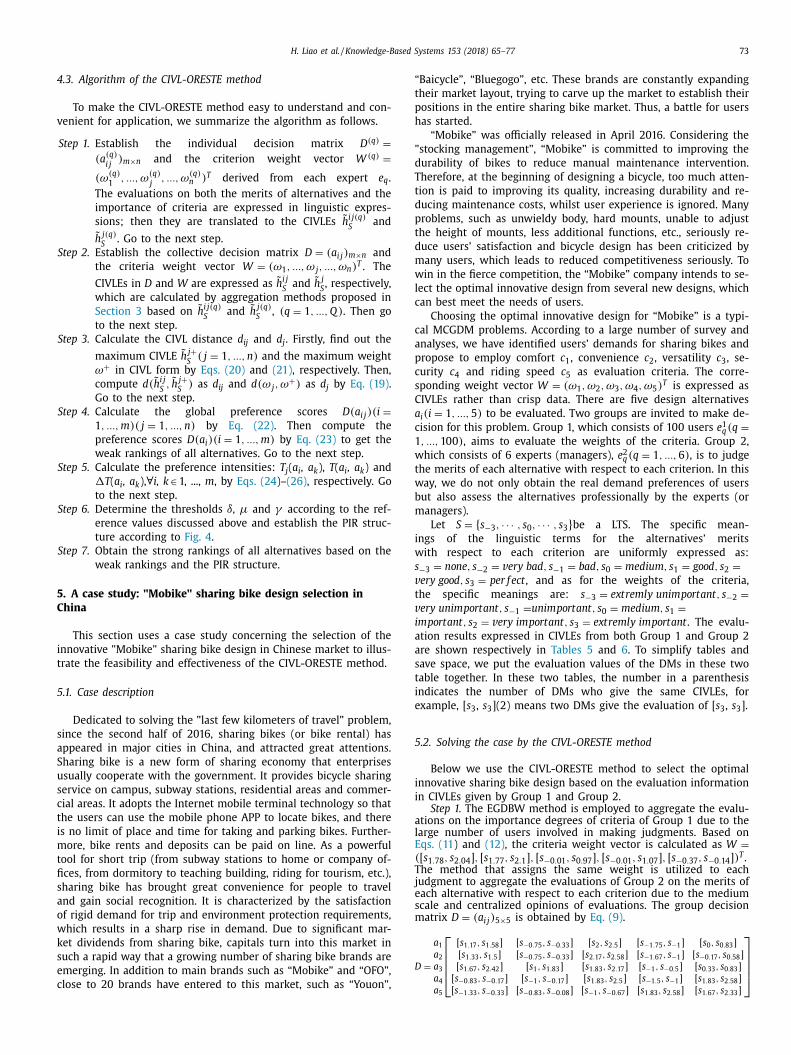
n CIVLEs given by Group 1 and Group 2. Step 1. The EGDBW method is employed to aggregate the evalu-
tions on the importance degrees of criteria of Group 1 due to thearge number of users involved in making judgments. Based onqs. (11 ) and (12) , the criteria weight vector is calculated as W =
([ s 1 . 78 , s 2 . 04 ] , [ s 1 . 77 , s 2 . 1 ] , [ s −0 . 01 , s 0 . 97 ] , [ s −0 . 01 , s 1 . 07 ] , [ s −0 . 37 , s −0 . 14 ]) T .
he method that assigns the same weight is utilized to eachudgment to aggregate the evaluations of Group 2 on the merits ofach alternative with respect to each criterion due to the mediumcale and centralized opinions of evaluations. The group decisionatrix D = ( a i j ) 5 ×5 is obtained by Eq. (9) .
=
a 1 a 2 a 3 a 4 a 5
⎡
⎢ ⎢ ⎢ ⎣
[ s 1 . 17 , s 1 . 58 ] [ s −0 . 75 , s −0 . 33 ] [ s 2 , s 2 . 5 ] [ s −1 . 75 , s −1 ] [ s 0 , s 0 . 83 ]
[ s 1 . 33 , s 1 . 5 ] [ s −0 . 75 , s −0 . 33 ] [ s 2 . 17 , s 2 . 58 ] [ s −1 . 67 , s −1 ] [ s −0 . 17 , s 0 . 58 ]
[ s 1 . 67 , s 2 . 42 ] [ s 1 , s 1 . 83 ] [ s 1 . 83 , s 2 . 17 ] [ s −1 , s −0 . 5 ] [ s 0 . 33 , s 0 . 83 ]
[ s −0 . 83 , s −0 . 17 ] [ s −1 , s −0 . 17 ] [ s 1 . 83 , s 2 . 5 ] [ s −1 . 5 , s −1 ] [ s 1 . 83 , s 2 . 58 ]
[ s −1 . 33 , s −0 . 33 ] [ s −0 . 83 , s −0 . 08 ] [ s −1 , s −0 . 67 ] [ s 1 . 83 , s 2 . 58 ] [ s 1 . 67 , s 2 . 33 ]
⎤⎥⎥⎥⎦

74 H. Liao et al. / Knowledge-Based Systems 153 (2018) 65–77
Table 5
The importance of the criteria evaluated by Group 1.
Importance
c 1 [ s 3 , s 3 ](2) [ s 2 , s 2.5 ](20) [ s 2 , s 2 ](48) [ s 1 , s 2 ](15) [ s 0 , s 1 ](10) [ s 0 , s 0 ](3) [ s −1 , s −1 ](2)
c 2 [ s 3 , s 3 ](5) [ s 2 , s 3 ](18) [ s 2 , s 2 ](45) [ s 1 , s 2 ](22) [ s 0 , s 1 ](7) [ s −1 , s 0 ](3) –
c 3 [ s 2 , s 3 ](1) [ s 2 , s 2 ](7) [ s 1 , s 1.5 ](16) [ s 0 , s 1 ](51) [ s −1 , s 0 ](20) [ s −2 , s 0 ](4) [ s −2 , s −1 ](1)
c 4 [ s 2 , s 3 ](3) [ s 2 , s 2.5 ](6) [ s 0 , s 2 ](21) [ s 0 , s 1 ](45) [ s 0 , s 0 ](20) [ s −1 , s −0 . 5 ](4) [ s −2 , s 0 ](1)
c 5 [ s 2 , s 3 ](2) [ s 1.5 , s 2 ](3) [ s 0 , s 1 ](14) [ s 0 , s 0 ](41) [ s −1 , s −0 . 5 ](26) [ s −2 , s −1 ](14) –
Table 6
The judgments on the alternatives under criteria given by Group 2.
c 1 c 2 c 3
a 1 [ s 2 , s 3 ](1), [ s 1 , s 1.5 ](3), [ s 1 , s 1 ](2) [ s 0 , s 0 ](1) , [ s −0 . 5 , s 0 ](3) , [ s −1 , s −1 ](1) , [ s −2 , s −1 ](1) [ s 2 , s 3 ](1), [ s 2 , s 2.5 ](4), [ s 2 , s 2 ](1)
a 2 [ s 2 , s 2 ](2), [ s 1 , s 1.5 ](2), [ s 1 , s 1 ](2) [ s 0 , s 0 ](1) , [ s −0 . 5 , s 0 ](3) , [ s −1 . 5 , s −1 ](2) [ s 2.5 , s 3 ](2), [ s 2 , s 2.5 ](3), [ s 2 , s 2 ](1)
a 3 [ s 2 , s 3 ](1), [ s 2 , s 2.5 ](3), [ s 1 , s 2 ](2) [ s 1 , s 2 ](5), [ s 1 , s 1 ](1) [ s 2 , s 3 ](1), [ s 2 , s 2 ](3), [ s 1.5 , s 2 ](2)
a 4 [ s 0 , s 0 ](1) , [ s −1 , s 0 ](4) , [ s −1 , s −1 ](1) [ s 0 , s 0 ](1) , [ s −1 , s 0 ](4) , [ s −2 , s −1 ](1) [ s 2 , s 3 ](1), [ s 2 , s 2.5 ](4), [ s 1 , s 2 ](1)
a 5 [ s −1 , s 0 ](4)[ s −2 , s −1 ](2) [ s 0 , s 0 ](1) , [ s −1 , s 0 ](4) , [ s −1 , s −0 . 5 ](1) [ s −1 , s 0 ](2) , [ s −1 , s −1 ](4) ,
c 4 c 5 a 1 [ s −1 . 5 , s −1 ](3) , [ s −2 , s −1 ](3) [ s 0 , s 1 ](5), [ s 0 , s 0 ](1)
a 2 [ s −1 , s −1 ](2) , [ s −2 , s −1 ](4) [ s 0 , s 1 ](2) , [ s 0 , s 0 . 5 ](3) , [ s −1 , s 0 ](1)
a 3 [ s −1 , s 0 ](3) , [ s −1 , s −1 ](3) [ s 1 , s 1 ](1), [ s 0.5 , s 1 ](2), [ s 0 , s 1 ](2), [ s 0 , s 0 ](1)
a 4 [ s −1 , s −1 ](3) , [ s −2 , s −1 ](3) [ s 2 , s 3 ](2), [ s 2 , s 2.5 ](3), [ s 1 , s 2 ](1)
a 5 [ s 2 , s 3 ](2), [ s 2 , s 2.5 ](3), [ s 1 , s 2 ](1) [ s 2 , s 3 ](2), [ s 2 , s 2 ](2), [ s 1 , s 2 ](2)
Table 7
The distances from each alternative to the best one under each
criterion.
Distance c 1 c 2 c 3 c 4 c 5
a 1 0.1152 0.3276 0.0221 0.5967 0.2984
a 2 0.1156 0.3276 0 0.5900 0.3333
a 3 0 0 0.0628 0.4929 0.2716
a 4 0.4242 0.3333 0.0412 0.5762 0
a 5 0.4796 0.3117 0.5350 0 0.035
Table 8
The global preference scores of CIVL-ORESTE.
Global score c 1 c 2 c 3 c 4 c 5
a 1 0.0816 0.2316 0.1764 0.4554 0.3334
a 2 0.0819 0.2316 0.1757 0.4510 0.3496
a 3 0.0051 0 0.1812 0.3884 0.3218
a 4 0.30 0 0 0.2357 0.1781 0.4420 0.2582
a 5 0.3392 0.2204 0.4171 0.1714 0.2593
Table 9
The weak ranking of the alternatives of CIVL-ORESTE.
Alternative a 1 a 2 a 3 a 4 a 5
Score 0.25568 0.25796 0.1793 0.2828 0.28148
Weak ranking 2 3 1 5 4
Fig. 5. The strong ranking between the designs resulted from the CIVL-ORESTE
method.
μ
t
r
5
c
S
5
t
a
0
γ
a
C
b
c
m
Step 2. By Eqs. (20 ) and (21) , find out the maxi-
mum weight ω
+ = [ s 1 . 77 , s 2 . 1 ] and the maximum CIVLEs of
the alternatives with respect to each criterion, which are˜ h 1+
S = [ s 1 . 67 , s 2 . 42 ] , ˜ h 2+
S = [ s 1 , s 1 . 83 ] , ˜ h 3+
S = [ s 2 . 17 , s 2 . 58 ] , ˜ h 4+
S = [ s 1 . 83 , s 2 . 58 ] ,
˜ h 5+ S
= [ s 1 . 83 , s 2 . 58 ] , respectively. According to Eq. (19) , we ob-
tain the distance d j ( j = 1 , ..., 5) from each criterion to the
most importance criterion as: d 1 = 0 . 0072 , d 2 = 0 , d 3 = 0 . 2485 ,
d 4 = 0 . 2424 , d 5 = 0 . 3651 and the distances d i j (i = 1 , ..., 5)
( j = 1 , ..., 5) from each alternative to the best one under each
criterion, which are shown in Table 7 .
Step 3. The global preference scores are shown in Table 8 com-
puted by Eq. (22) based on d ij and d j . The weak ranking of all al-
ternatives is shown in Table 9 computed by Eq. (23) .
Steps 4 and 5. Calculate the preference intensities by Eqs. (24 )–
(26) . Let δ= 0 . 03 in this case. Then we obatin γ =
(n +2) δ = 0 . 021 and
2 n=
δn = 0 . 006 .The average preference intensities and the PIR rela-
ions of the “Mobike” innovative designs are shown in Table 10 .
Step 6. The strong ranking of all alternatives based on the weak
anking and the PIR structure is shown in Fig. 5 .
.3. Solving the case by the classical ORESTE method
Below we solve the case by the classical ORESTE method. Ac-
ording to the alternatives’ distance table ( Table 8 ) obtained in
tep 2 of the CIVL-ORETSE method, we get the ranks r j (1, 2, ...,
) of the criteria for the importance degrees and the ranks r j ( a i )
(i = 1 , 2 , ..., 5) of the alternatives with respect to each criterion for
heir merits. The average preference intensities between pairwise
lternatives are shown in Table 11 .
Let ˜ δ = 2 . Then according to Eq. (18) , we get ˜ μ < 1 / ( m − 1 ) n = . 05 , ˜ γ <
˜ δ/ 2(m − 1) = 0 . 25 , λ > (n − 2) / 4 = 0 . 75 . Let ˜ μ = 0 . 04 ,
˜ = 0 . 15 and λ = 2 in this paper, we get a 1 R a 4 , a 1 R a 5 , a 2 R a 5 and
4 R a 5 .
The strong ranking is shown in Fig. 6 .
Comparative analysis: There are different results derived by the
IVL-ORESTE and the ORESTE methods. The ORESTE method has
een improved by three aspects: the evaluation information in de-
ision matrix, the calculation processes and the technique to deter-
ine the thresholds, which are described in details as follows:
(1) With regard to the initial calculation data derived from
evaluation information, the CIVL-ORESTE method maintains
more evaluation information by employing the distance d j

H. Liao et al. / Knowledge-Based Systems 153 (2018) 65–77 75
Table 10
The average preference intensities between pairwise alternatives.
a 1 a 2 a 3 a 4 a 5
T ( a 1 , a i ) Relation T ( a 2 , a i ) Relation T ( a 3 , a i ) Relation T ( a 4 , a i ) Relation T ( a 5 , a i ) Relation
a 1 0 – 0.00102 I 0.07734 > 0.01772 < 0.07386 <
a 2 0.0033 I 0 – 0.07976 > 0.02008 < 0.07622 <
a 3 0.0 0 096 < 0.0011 < – – 0.01334 < 0.0559 <
a 4 0.04484 > 0.04492 > 0.11684 > – – 0.05718 R
a 5 0.09966 > 0.09974 > 0.15808 > 0.05586 R – –
Table 11
The average preference intensities between pairwise alter-
natives of the ORESTE method.
Intensity a 1 a 2 a 3 a 4 a 5
a 1 – 0.095 0.26 0.175 0.275
a 2 0.04 – 0.23 0.07 0.22
a 3 0.075 0.1 – 0.105 0.045
a 4 0.185 0.185 0.3 – 0.2
a 5 0.255 0.255 0.21 0.17 –
Fig. 6. The strong ranking between the alternatives resulted from the ORESTE
method.
Table 12
The results derived by the CIVL-VIKOR method.
a 1 a 2 a 3 a 4 a 5
GU i 0.6186 0.6240 0.2839 0.6588 0.6785
RS i 0.2457 0.2457 0.1487 0.25 0.25
Utility values 0.9029 0.9097 0 0.975 1
Rank 2 3 1 4 5
5
w
a
c
m
p
W
n
r
p
I
t
∑
d
w
a
s
m
m
t
and d ij rather than the Besson’s mean ranks r j and r j ( a i ).
In the above case study, from the decision matrix, we can
find that the evaluation of a 11 is extremely close to a 21 but
a 41 is far away to a 21 . These similarities and differences are
clearly reflected by the distances: d 11 = 0 . 1152 , d 21 = 0 . 1156
and d 41 = 0 . 4242 , but they are obscured by the Besson’s
mean ranks: r 1 ( a 1 ) = 2 , r 1 ( a 2 ) = 3 and r 1 ( a 4 ) = 4 .
(2) With regard to the weak ranking, the ORESTE method con-
verts the global preference score ˜ D ( a i j ) into the global weak
rank r ( a ij ) to calculate the weak rank R ( a i ), which leads to
information loss. For example by Eq. (14) we have ˜ D ( a 32 ) =1 corresponding to r( a 32 ) = 1 , ˜ D ( a 31 ) = 1 . 5811 to r( a 31 ) =2 . 5 , ˜ D ( a 21 ) = 2 . 5495 to r( a 21 ) = 6 . 5 , and
˜ D ( a 22 ) = 2 . 5739 to
r( a 22 ) = 8.5. It is clear that the global weak rank weakens
the score information that ˜ D ( a 31 ) − ˜ D ( a 32 ) = 0 . 5811 related
to r( a 31 ) − r( a 32 ) = 1 . 5 but ˜ D ( a 22 ) − ˜ D ( a 21 ) = 0 . 0244 related
to r( a 22 ) − r( a 21 ) = 2 . However, in the CIVL-ORESTE method,
the weak rank r ( a i ) is derived by the global preference score
D ( a ij ) directly.
(3) With regard to the preference intensities, they are computed
by the global weak ranking in the classical ORESTE method
while by the global preference scores in the CIVL-ORESTE
method. From the above discussion, we can make a conclu-
sion that the preference intensities of the ORESTE method
are untrustworthy due to the less information in the global
weak ranking.
(4) With regard to the thresholds, in the ORESTE method, ˜ δ are
determined by the DM freely with less basis and the ranges
of thresholds are so broad that it is difficult to choose rea-
sonable values, which has a decisive effect on the results.
For the above case, if ˜ γ ∈ [0 , 0 . 185) , a 1 R a 4 and a 4 R a 5 ; if
˜ γ ∈ [0 . 185 , 0 . 2) , a 1 I a 4 and a 4 R a 5 ; if ˜ γ ∈ [0 . 2 , 0 . 25) , a 1 I a 4and a 4 I a 5 . However, in the CIVL-ORESTE method, the in-
difference threshold δ is derived based on the distance be-
tween two CIVLEs, and the other two thresholds μ and γare calculated by δ, which forms a systematic process to set
the values of these parameters to ensure that the rankings
are generated consistently. Furthermore, they vary in smaller
ranges and as the value changes, the results are stable. In
the case study, if δ ∈ [0, 0.0336], the results obtained will be
similar.
.4. Solving the case by other ranking methods
To further illustrate the reliability of the CIVL-ORESTE method,
e deal with the case by three widely used ranking methods
nd make some comparative analyses. Considering that the crisp
riterion weights are the basis of these methods, we can deter-
ine the weights based on the evaluations of criteria by a sim-
le formula ˜ ω j = d ( h j S , min
j
˜ h j S ) /
∑ n j=1 d (
h j S , min
j
˜ h j S ) , and thus obtain
= (0 . 25 , 0 . 25 , 0 . 18 , 0 . 18 , 0 . 14) T .
(1) The results derived by the CIVL-VIKOR method
As a utility value-based ranking method, the VIKOR ranks alter-
atives considering both the group utility values and the individual
egret values. It can avoid the defect that the selected solution may
erform badly under some criteria as in the TOPSIS method [22] .
n this part, we extend the VIKOR to the CIVL context to handle
he case.
The group utility values can be calculated by G U i = n j=1 ˜ ω j ( d i j / max
i d i j ) and the individual regret values can be
etermined by R S i = max j
˜ ω j ( d i j / max i
d i j ) where ˜ ω j is the crisp
eight of criterion c j . Let the relative importance between GU i
nd RS i be 0.5. The results derived by the CIVL-VIKOR method are
hown in Table 12 .
Comparative analysis: The results derived by the CIVL-VIKOR
ethod are like the weak ranking obtained by the CIVL-ORESTE
ethod. But the CIVL-VIKOR cannot describe a detail relation be-
ween pairwise alternatives. It deems that alternative a is superior
1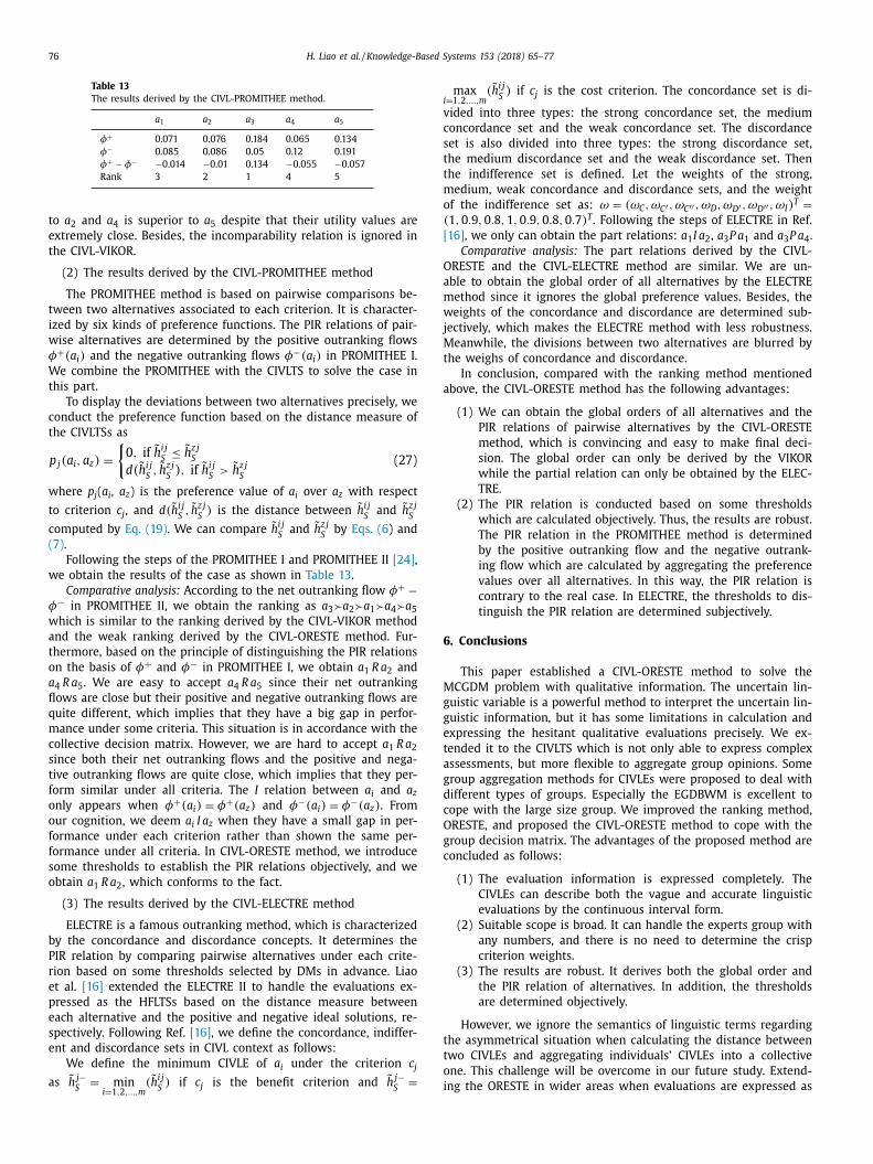
76 H. Liao et al. / Knowledge-Based Systems 153 (2018) 65–77
Table 13
The results derived by the CIVL-PROMITHEE method.
a 1 a 2 a 3 a 4 a 5
φ+ 0.071 0.076 0.184 0.065 0.134
φ− 0.085 0.086 0.05 0.12 0.191
φ+ − φ− −0.014 −0.01 0.134 −0.055 −0.057
Rank 3 2 1 4 5
i
v
c
s
t
t
m
o
[
O
a
m
w
j
M
t
a
6
M
g
g
e
t
a
g
d
c
O
g
c
t
t
o
i
to a 2 and a 4 is superior to a 5 despite that their utility values are
extremely close. Besides, the incomparability relation is ignored in
the CIVL-VIKOR.
(2) The results derived by the CIVL-PROMITHEE method
The PROMITHEE method is based on pairwise comparisons be-
tween two alternatives associated to each criterion. It is character-
ized by six kinds of preference functions. The PIR relations of pair-
wise alternatives are determined by the positive outranking flows
φ+ ( a i ) and the negative outranking flows φ−( a i ) in PROMITHEE I.
We combine the PROMITHEE with the CIVLTS to solve the case in
this part.
To display the deviations between two alternatives precisely, we
conduct the preference function based on the distance measure of
the CIVLTSs as
p j ( a i , a z ) =
{0 , if ˜ h
i j S
≤ ˜ h
z j S
d( h
i j S , h
z j S ) , if ˜ h
i j S
>
˜ h
z j S
(27)
where p j ( a i , a z ) is the preference value of a i over a z with respect
to criterion c j , and d( h i j S , h
z j S
) is the distance between
˜ h i j S
and
˜ h z j S
computed by Eq. (19) . We can compare ˜ h i j S
and
˜ h z j S
by Eqs. (6 ) and
(7) .
Following the steps of the PROMITHEE I and PROMITHEE II [24] ,
we obtain the results of the case as shown in Table 13 .
Comparative analysis: According to the net outranking flow φ+ −φ− in PROMITHEE II, we obtain the ranking as a 3 �a 2 �a 1 �a 4 �a 5 which is similar to the ranking derived by the CIVL-VIKOR method
and the weak ranking derived by the CIVL-ORESTE method. Fur-
thermore, based on the principle of distinguishing the PIR relations
on the basis of φ+ and φ− in PROMITHEE I, we obtain a 1 R a 2 and
a 4 R a 5 . We are easy to accept a 4 R a 5 since their net outranking
flows are close but their positive and negative outranking flows are
quite different, which implies that they have a big gap in perfor-
mance under some criteria. This situation is in accordance with the
collective decision matrix. However, we are hard to accept a 1 R a 2 since both their net outranking flows and the positive and nega-
tive outranking flows are quite close, which implies that they per-
form similar under all criteria. The I relation between a i and a z only appears when φ+ ( a i ) = φ+ ( a z ) and φ−( a i ) = φ−( a z ) . From
our cognition, we deem a i I a z when they have a small gap in per-
formance under each criterion rather than shown the same per-
formance under all criteria. In CIVL-ORESTE method, we introduce
some thresholds to establish the PIR relations objectively, and we
obtain a 1 R a 2 , which conforms to the fact.
(3) The results derived by the CIVL-ELECTRE method
ELECTRE is a famous outranking method, which is characterized
by the concordance and discordance concepts. It determines the
PIR relation by comparing pairwise alternatives under each crite-
rion based on some thresholds selected by DMs in advance. Liao
et al. [16] extended the ELECTRE II to handle the evaluations ex-
pressed as the HFLTSs based on the distance measure between
each alternative and the positive and negative ideal solutions, re-
spectively. Following Ref. [16] , we define the concordance, indiffer-
ent and discordance sets in CIVL context as follows:
We define the minimum CIVLE of a i under the criterion c j
as ˜ h j−S
= min
i =1 , 2 ,...,m
( h i j S ) if c j is the benefit criterion and
˜ h j−S
=
max =1 , 2 ,...,m
( h i j S ) if c j is the cost criterion. The concordance set is di-
ided into three types: the strong concordance set, the medium
oncordance set and the weak concordance set. The discordance
et is also divided into three types: the strong discordance set,
he medium discordance set and the weak discordance set. Then
he indifference set is defined. Let the weights of the strong,
edium, weak concordance and discordance sets, and the weight
f the indifference set as: ω = ( ω C , ω C ′ , ω C ′′ , ω D , ω D ′ , ω D ′′ , ω I ) T =
(1 , 0 . 9 , 0 . 8 , 1 , 0 . 9 , 0 . 8 , 0 . 7) T . Following the steps of ELECTRE in Ref.
16] , we only can obtain the part relations: a 1 I a 2 , a 3 P a 1 and a 3 P a 4 .
Comparative analysis: The part relations derived by the CIVL-
RESTE and the CIVL-ELECTRE method are similar. We are un-
ble to obtain the global order of all alternatives by the ELECTRE
ethod since it ignores the global preference values. Besides, the
eights of the concordance and discordance are determined sub-
ectively, which makes the ELECTRE method with less robustness.
eanwhile, the divisions between two alternatives are blurred by
he weighs of concordance and discordance.
In conclusion, compared with the ranking method mentioned
bove, the CIVL-ORESTE method has the following advantages:
(1) We can obtain the global orders of all alternatives and the
PIR relations of pairwise alternatives by the CIVL-ORESTE
method, which is convincing and easy to make final deci-
sion. The global order can only be derived by the VIKOR
while the partial relation can only be obtained by the ELEC-
TRE.
(2) The PIR relation is conducted based on some thresholds
which are calculated objectively. Thus, the results are robust.
The PIR relation in the PROMITHEE method is determined
by the positive outranking flow and the negative outrank-
ing flow which are calculated by aggregating the preference
values over all alternatives. In this way, the PIR relation is
contrary to the real case. In ELECTRE, the thresholds to dis-
tinguish the PIR relation are determined subjectively.
. Conclusions
This paper established a CIVL-ORESTE method to solve the
CGDM problem with qualitative information. The uncertain lin-
uistic variable is a powerful method to interpret the uncertain lin-
uistic information, but it has some limitations in calculation and
xpressing the hesitant qualitative evaluations precisely. We ex-
ended it to the CIVLTS which is not only able to express complex
ssessments, but more flexible to aggregate group opinions. Some
roup aggregation methods for CIVLEs were proposed to deal with
ifferent types of groups. Especially the EGDBWM is excellent to
ope with the large size group. We improved the ranking method,
RESTE, and proposed the CIVL-ORESTE method to cope with the
roup decision matrix. The advantages of the proposed method are
oncluded as follows:
(1) The evaluation information is expressed completely. The
CIVLEs can describe both the vague and accurate linguistic
evaluations by the continuous interval form.
(2) Suitable scope is broad. It can handle the experts group with
any numbers, and there is no need to determine the crisp
criterion weights.
(3) The results are robust. It derives both the global order and
the PIR relation of alternatives. In addition, the thresholds
are determined objectively.
However, we ignore the semantics of linguistic terms regarding
he asymmetrical situation when calculating the distance between
wo CIVLEs and aggregating individuals’ CIVLEs into a collective
ne. This challenge will be overcome in our future study. Extend-
ng the ORESTE in wider areas when evaluations are expressed as
H. Liao et al. / Knowledge-Based Systems 153 (2018) 65–77 77
t
r
A
d
t
R
v
f
R
[
[
[
[
[
[
[
[
[
[
[
[
[
[
[
he hesitant fuzzy number and the intuitionistic multiplicative set
ather than linguistic term sets is also interesting.
cknowledgments
The work was supported by the National Natural Science Foun-
ation of China (no. 71771156 , no. 71501135 ,), the China Postdoc-
oral Science Foundation ( 2016T90863 , 2016M602698 ), the Sientific
esearch Foundation for Excellent Young Scholars at Sichuan Uni-
ersity(no. 2016SCU04A23 ), and the International Visiting Program
or Excellent Young Scholars of SCU.
eferences
[1] E.K. Zavadskas , Z. Turskis , Multiple criteria decision making (MCDM) methods
in economics: an overview, Technol. Econ. Dev. Econ. 17 (2) (2011) 397–427 . [2] E.K. Zavadskas , Z. Turskis , S. Kildien e , State of art surveys of overviews on
MCDM/MADM methods, Technol. Econ. Dev. Econ. 20 (1) (2014) 165–179 .
[3] M.X. Wang, J.Q Wang, New online recommendation approach based on un-balanced linguistic label with integrated cloud, Kybernetes (2018), doi: 10.1108/
K- 06- 2017- 0211 . [4] H.G Peng , H.Y Zhang , J.Q Wang , Cloud decision support model for selecting
hotels on TripAdvisor.com with probabilistic linguistic information, Int. J. Hosp.Manag. 68 (2018) 124–138 .
[5] L.A. Zadeh , The concept of a linguistic variable and its application to approxi-
mate reasoning-Part I, Inf. Sci. 8 (3) (1975) 199–249 . [6] F. Herrera , L. Martínez , A 2-tuple fuzzy linguistic representation model for
computing with words, IEEE Trans. Fuzzy Syst. 8 (20 0 0) 746–752 . [7] Z.S. Xu , Uncertain linguistic aggregation operators based approach to multiple
attribute group decision making under uncertain linguistic environment, Inf.Sci. 168 (1-4) (2004) 171–184 .
[8] H.C. Liao, Z.S. Xu, E. Herrera-Viedma, F. Herrera, Hesitant fuzzy linguistic term
set and its application in decision making: a state-of-the art survey, Int. J.Fuzzy Syst. (2018), doi: 10.1007/s40815- 017- 0432- 9 .
[9] I. Truck , Comparison and links between two 2-tuple linguistic models for de-cision making, Knowledge-Based Syst. 87 (2015) 61–68 .
[10] R.M. Rodríguez , L. Martınez , F. Herrera , Hesitant fuzzy linguistic terms sets fordecision making, IEEE Trans. Fuzzy Syst. 20 (2012) 109–119 .
[11] H.C. Liao , Z.S. Xu , X.J. Zeng , J.M. Merigó, Qualitative decision making with cor-
relation coefficients of hesitant fuzzy linguistic term sets, Knowledge-BasedSyst. 76 (2015) 127–138 .
[12] R.X Liang , J.Q Wang , H.Y Zhang , Projection-based PROMETHEE methods basedon hesitant fuzzy linguistic term sets, Int. J. Fuzzy Syst. (2017) 1–14 .
[13] J.Q. Wang , J.T. Wu , J. Wang , H.Y. Zhang , X.H. Chen , Interval-valued hesitantfuzzy linguistic sets and their applications in multi-criteria decision-making
problems, Inf. Sci. 288 (2014) 55–72 .
[14] Z.S. Chen , K.S. Chin , Y.L. Li , Y. Yang , Proportional hesitant fuzzy linguistic termset for multiple criteria group decision making, Inf. Sci. 357 (2016) 61–87 .
[15] J.Q. Wang , J. Wang , Q.H. Chen , H.Y. Zhang , X.H. Chen , An outranking approachfor multi-criteria decision-making with hesitant fuzzy linguistic term sets, Inf.
Sci. 280 (2014) 338–351 . [16] H.C. Liao , L.Y. Yang , Z.S. Xu , Two new approaches based on ELECTRE II to solve
the multiple criteria decision making problems with hesitant fuzzy linguistic
term sets, Appl. Soft Comput. 63 (2018) 223–234 .
[17] H.C. Liao , Z.S. Xu , X.J. Zeng , Distance and similarity measures for hesitant fuzzylinguistic term sets and their application in multi-criteria decision making, Inf.
Sci. 271 (2014) 125–142 . [18] J.D Qin , X.W Liu , W. Pedrycz , An extended VIKOR method based on prospect
theory for multiple attribute decision making under interval type-2 fuzzy en-vironment, Knowledge-Based Syst. 86 (C) (2015) 116–130 .
[19] X.L. Wu , H.C. Liao , An approach to quality function deployment based on prob-abilistic linguistic term sets and ORESTE method for multi-expert multi-criteria
decision making, Inf. Fusion 43 (2018) 13–26 .
20] Z.S. Xu , An overview of methods for determining OWA weights, Int. J. Intell.Syst. 20 (8) (2005) 843–865 .
[21] L. Dymova , P. Sevastjanov , A. Tikhonenko , An interval type-2 fuzzy extensionof the TOPSIS method using alpha cuts, Knowledge-Based Syst. 83 (1) (2015)
116–127 . 22] S. Opricovic , G.H. Tzeng , Compromise solution by MCDM methods: a compar-
ative analysis of VIKOR and TOPSIS, Eur. J. Oper. Res. 156 (2) (2004) 445–455 .
23] H. Ma , H.B. Zhu , Z.G. Hu , K.Q. Li , W.S. Tang , Time-aware trustworthiness rank-ing prediction for cloud services using interval neutrosophic set and ELECTRE,
Knowledge-Based Syst. 138 (2017) 27–45 . 24] J.P. Brans , B. Mareschal , Promethee methods, Mult.e Criteria Decis. Anal. State
Art Surv. (2013) 163–186 . 25] M. Roubens , Preference relations an actions and criteria in multicriteria deci-
sion making, Eur. J. Oper. Res. 10 (1) (1982) 51–55 .
26] H. Wang , Extended hesitant fuzzy linguistic term sets and their aggregation ingroup decision making, Int. J. Comput. Intell. Syst. 8 (1) (2015) 14–33 .
[27] E. Herrera-Viedma , Fuzzy sets and fuzzy logic in multi-criteria decision mak-ing. The 50th anniversary of Prof. Lotfi Zadeh’s theory: introduction, Technol.
Econ. Develop. Econ. 21 (5) (2015) 677–683 . 28] C.A. Franco , On the analytic hierarchy process and decision support based
on fuzzy-linguistic preference structures, Knowledge-Based Syst. 70 (2014)
203–211 . 29] F.F. Jin , L.D. Pei , H.Y. Chen , L.G. Zhou , Interval-valued intuitionistic fuzzy con-
tinuous weighted entropy and its application to multi-criteria fuzzy group de-cision making, Knowledge-Based Syst. 59 (2) (2014) 132–141 .
30] S.M. Yu, J Wang, J.Q. Wang, L. Li, A multi-criteria decision-making model forhotel selection with linguistic distribution assessments, Appl. Soft Comput.
(2017), doi: 10.1016/j.asoc.2017.08.009 .
[31] B. Liu , Y. Shen , Y. Chen , X. Chen , Y. Wang , A two-layer weight determinationmethod for complex multi-attribute large-group decision-making experts in a
linguistic environment, Inf. Fusion 23 (2015) 156–165 . 32] B. Bourguignon , D.L. Massart , The Oreste method for multicriteria decision
making in experimental chemistry, Chemom. Intell. Lab. Syst. 22 (2) (1994)241–256 .
33] H. Pastijn , J. Leysen , Constructing an outranking relation with ORESTE, Math.
Comput. Modell. 12 (10-11) (1989) 1255–1268 . 34] C. Delhaye , J. Teghem , P. Kunsch , Application of the ORESTE method to a nu-
clear waste management problem, Int. J. Prod. Econ. 24 (1-2) (1991) 29–39 . 35] G.V. Huylenbroeck , The conflict analysis method: bridging the gap between
ELECTRE, PROMETHEE and ORESTE, Eur. J. Oper. Res. 82 (3) (1995) 490–502 . 36] I.D. Leeneer , H. Pastijn , Selecting land mine detection strategies by means of
outranking MCDM techniques, Eur. J. Oper. Res. 139 (2) (2002) 327–338 . [37] E.A . Adali , A .T. Isik , Ranking web design firms with the ORESTE mthod, Ege
Acad. Rev. 17 (2) (2017) 243–253 .
38] M.A. Yerlikaya , F. Arikan , Constructing the performance effectiveness order ofsme supports programmes via Promethee and Oreste techniques, J. Faculty
Eng. Architect. Gazi Univ. 31 (4) (2016) 1007–1016 .