Embed Size (px)
Citation preview

Journal of Artificial Intelligence Research 25 (2006) 457-502 Submitted 11/05; published 4/06
A Continuation Method for Nash Equilibria in StructuredGames
Ben Blum [email protected] of California, BerkeleyDepartment of Electrical Engineering and Computer ScienceBerkeley, CA 94720
Christian R. Shelton [email protected] of California, RiversideDepartment of Computer Science and EngineeringRiverside, CA 92521
Daphne Koller [email protected]
Stanford UniversityDepartment of Computer ScienceStanford, CA 94305
Abstract
Structured game representations have recently attracted interest as models for multi-agent artificial intelligence scenarios, with rational behavior most commonly characterizedby Nash equilibria. This paper presents efficient, exact algorithms for computing Nash equi-libria in structured game representations, including both graphical games and multi-agentinfluence diagrams (MAIDs). The algorithms are derived from a continuation method fornormal-form and extensive-form games due to Govindan and Wilson; they follow a trajec-tory through a space of perturbed games and their equilibria, exploiting game structurethrough fast computation of the Jacobian of the payoff function. They are theoreticallyguaranteed to find at least one equilibrium of the game, and may find more. Our approachprovides the first efficient algorithm for computing exact equilibria in graphical games witharbitrary topology, and the first algorithm to exploit fine-grained structural properties ofMAIDs. Experimental results are presented demonstrating the effectiveness of the algo-rithms and comparing them to predecessors. The running time of the graphical gamealgorithm is similar to, and often better than, the running time of previous approximatealgorithms. The algorithm for MAIDs can effectively solve games that are much largerthan those solvable by previous methods.
1. Introduction
In attempting to reason about interactions between multiple agents, the artificial intelligencecommunity has recently developed an interest in game theory, a tool from economics. Gametheory is a very general mathematical formalism for the representation of complex multi-agent scenarios, called games, in which agents choose actions and then receive payoffs thatdepend on the outcome of the game. A number of new game representations have beenintroduced in the past few years that exploit structure to represent games more efficiently.These representations are inspired by graphical models for probabilistic reasoning from theartificial intelligence literature, and include graphical games (Kearns, Littman, & Singh,
c©2006 AI Access Foundation. All rights reserved.

Blum, Shelton, & Koller
2001), multi-agent influence diagrams (MAIDs) (Koller & Milch, 2001), G nets (La Mura,2000), and action-graph games (Bhat & Leyton-Brown, 2004).
Our goal is to describe rational behavior in a game. In game theory, a description of thebehavior of all agents in the game is referred to as a strategy profile: a joint assignment ofstrategies to each agent. The most basic criterion to look for in a strategy profile is that it beoptimal for each agent, taken individually: no agent should be able to improve its utility bychanging its strategy. The fundamental game theoretic notion of a Nash equilibrium (Nash,1951) satisfies this criterion precisely. A Nash equilibrium is a strategy profile in whichno agent can improve its payoff by deviating unilaterally — changing its strategy while allother agents hold theirs fixed. There are other types of game theoretic solutions, but theNash equilibrium is the most fundamental and is often agreed to be a minimum solutionrequirement.
Computing equilibria can be difficult for several reasons. First, game representationsthemselves can grow quite large. However, many of the games that we would be interestedin solving do not require the full generality of description that leads to large representationsize. The structured game representations introduced in AI exploit structural propertiesof games to represent them more compactly. Typically, this structure involves locality ofinteraction — agents are only concerned with the behavior of a subset of other agents.
One would hope that more compact representations might lead to more efficient compu-tation of equilibria than would be possible with standard game-theoretic solution algorithms(such as those described by McKelvey & McLennan, 1996). Unfortunately, even with com-pact representations, games are quite hard to solve; we present a result showing that findingNash equilibria beyond a single trivial one is NP-hard in the types of structured games thatwe consider.
In this paper, we describe a set of algorithms for computing equilibria in structuredgames that perform quite well, empirically. Our algorithms are in the family of continuationmethods. They begin with a solution of a trivial perturbed game, then track this solution asthe perturbation is incrementally undone, following a trajectory through a space of equilibriaof perturbed games until an equilibrium of the original game is found. Our algorithms arebased on the recent work of Govindan and Wilson (2002, 2003, 2004) (GW hereafter),which applies to standard game representations (normal-form and extensive-form). Thealgorithms of GW are of great interest to the computational game theory community intheir own right; Nudelman et al. (2004) have tested them against other leading algorithmsand found them, in certain cases, to be the most effective available. However, as withall other algorithms for unstructured games, they are infeasible for very large games. Weshow how game structure can be exploited to perform the key computational step of thealgorithms of GW, and also give an alternative presentation of their work.
Our methods address both graphical games and MAIDs. Several recent papers havepresented methods for finding equilibria in graphical games. Many of the proposed algo-rithms (Kearns et al., 2001; Littman, Kearns, & Singh, 2002; Vickrey & Koller, 2002; Ortiz& Kearns, 2003) have focused on finding approximate equilibria, in which each agent mayin fact have a small incentive to deviate. These sorts of algorithms can be problematic:approximations must be crude for reasonable running times, and there is no guarantee ofan exact equilibrium in the neighborhood of an approximate one. Algorithms that findexact equilibria have been restricted to a narrow class of games (Kearns et al., 2001). We
458

A Continuation Method for Nash Equilibria in Structured Games
present the first efficient algorithm for finding exact equilibria in graphical games of ar-bitrary structure. We present experimental results showing that the running time of ouralgorithm is similar to, and often better than, the running time of previous approximatealgorithms. Moreover, our algorithm is capable of using approximate algorithms as startingpoints for finding exact equilibria.
The literature for MAIDs is more limited. The algorithm of Koller and Milch (2001)only takes advantage of certain coarse-grained structure in MAIDs, and otherwise fallsback on generating and solving standard extensive-form games. Methods for related typesof structured games (La Mura, 2000) are also limited to coarse-grained structure, andare currently unimplemented. Approximate approaches for MAIDs (Vickrey, 2002) comewithout implementation details or timing results. We provide the first exact algorithm thatcan take advantage of the fine-grained structure of MAIDs. We present experimental resultsdemonstrating that our algorithm can solve MAIDs that are significantly outside the scopeof previous methods.
1.1 Outline and Guide to Background Material
Our results require background in several distinct areas, including game theory, continuationmethods, representations of graphical games, and representation and inference for Bayesiannetworks. Clearly, it is outside the scope of this paper to provide a detailed review of all ofthese topics. We have attempted to provide, for each of these topics, sufficient backgroundto allow our results to be understood.
We begin with an overview of game theory in Section 2, describing strategy represen-tations and payoffs in both normal-form games (single-move games) and extensive-formgames (games with multiple moves through time). All concepts utilized in this paper willbe presented in this section, but a more thorough treatment is available in the standardtext by Fudenberg and Tirole (1991). In Section 3 we introduce the two structured gamerepresentations addressed in this paper: graphical games (derived from normal-form games)and MAIDs (derived from extensive-form games). In Section 4 we give a result on the com-plexity of computing equilibria in both graphical games and MAIDs, with the proof deferredto Appendix B. We next outline continuation methods, the general scheme our algorithmsuse to compute equilibria, in Section 5. Continuation methods form a broad computationalframework, and our presentation is therefore necessarily limited in scope; Watson (2000)provides a more thorough grounding. In Section 6 we describe the particulars of applyingcontinuation methods to normal-form games and to extensive-form games. The presentationis new, but the methods are exactly those of GW.
In Section 7, we present our main contribution: exploiting structure to perform thealgorithms of GW efficiently on both graphical games and MAIDs. We show how Bayesiannetwork inference in MAIDs can be used to perform the key computational step of the GWalgorithm efficiently, taking advantage of finer-grained structure than previously possible.Our algorithm utilizes, as a subroutine, the clique tree inference algorithm for Bayesiannetworks. Although we do not present the clique tree method in full, we describe theproperties of the method that allow it to be used within our algorithm; we also provideenough detail to allow an implementation of our algorithm using a standard clique treepackage as a black box. For a more comprehensive introduction to inference in Bayesian
459

Blum, Shelton, & Koller
networks, we refer the reader to the reference by Cowell, Dawid, Lauritzen, and Spiegelhalter(1999). In Section 8, we present running-time results for a variety of graphical games andMAIDs. We conclude in Section 9.
2. Game Theory
We begin by briefly reviewing concepts from game theory used in this paper, referring tothe text by Fudenberg and Tirole (1991) for a good introduction. We use the notationemployed by GW. Those readers more familiar with game theory may wish to skip directlyto the table of notation in Appendix A.
A game defines an interaction between a set N = {n1, n2, . . . , n|N |} of agents. Each agentn ∈ N has a set Σn of available strategies, where a strategy determines the agent’s behaviorin the game. The precise definition of the set Σn depends on the game representation, aswe discuss below. A strategy profile σ = (σn1 , σn2 , . . . , σn|N|) ∈
∏n∈N Σn defines a strategy
σn ∈ Σn for each agent n ∈ N . Given a strategy profile σ, the game defines an expectedpayoff Gn(σ) for each agent n ∈ N . We use Σ−n to refer to the set of all strategy profilesof agents in N \ {n} (agents other than n) and σ−n ∈ Σ−n to refer to one such profile; wegeneralize this notation to Σ−n,n′ for the set of strategy profiles of all but two agents. If σis a strategy profile, and σ′n ∈ Σn is a strategy for agent n, then (σ′n, σ−n) is a new strategyprofile in which n deviates from σ to play σ′n, and all other agents act according to σ.
A solution to a game is a prescription of a strategy profile for the agents. In this paper,we use Nash equilibria as our solution concept — strategy profiles in which no agent canprofit by deviating unilaterally. If an agent knew that the others were playing accordingto an equilibrium profile (and would not change their behavior), it would have no incentiveto deviate. Using the notation we have outlined here, we can define a Nash equilibriumto be a strategy profile σ such that, for all n ∈ N and all other strategies σ′n ∈ Σn,Gn(σn, σ−n) ≥ Gn(σ′n, σ−n).
We can also define a notion of an approximate equilibrium, in which each agent’s in-centive to deviate is small. An ε-equilibrium is a strategy profile σ such that no agentcan improve its expected payoff by more than ε by unilaterally deviating from σ. In otherwords, for all n ∈ N and all other strategies σ′n ∈ Σn, Gn(σ′n, σ−n) − Gn(σn, σ−n) ≤ ε.Unfortunately, finding an ε-equilibrium is not necessarily a step toward finding an exactequilibrium: the fact that σ is an ε-equilibrium does not guarantee the existence of an exactequilibrium in the neighborhood of σ.
2.1 Normal-Form Games
A normal-form game defines a simultaneous-move multi-agent scenario. Each agent inde-pendently selects an action and then receives a payoff that depends on the actions selectedby all of the agents. More precisely, let G be a normal-form game with a set N of agents.Each agent n ∈ N has a discrete action set An and a payoff array Gn with entries for everyaction profile in A =
∏n∈N An — that is, for joint actions a = (an1 , an2 , . . . , an|N|) of all
agents. We use A−n to refer to the joint actions of agents in N \ {n}.
460

A Continuation Method for Nash Equilibria in Structured Games
2.1.1 Strategy Representation
If agents are restricted to choosing actions deterministically, an equilibrium is not guaran-teed to exist. If, however, agents are allowed to independently randomize over actions, thenthe seminal result of game theory (Nash, 1951) guarantees the existence of a mixed strategyequilibrium. A mixed strategy σn is a probability distribution over An.
The strategy set Σn is therefore defined to be the probability simplex of all mixedstrategies. The support of a mixed strategy is the set of actions in An that have non-zeroprobability. A strategy σn for agent n is said to be a pure strategy if it has only a singleaction in its support — pure strategies correspond exactly to the deterministic actions inAn. The set Σ of mixed strategy profiles is
∏n∈N Σn, a product of simplices. A mixed
strategy for a single agent can be represented as a vector of probabilities, one for eachaction. For notational simplicity later on, we can concatenate all these vectors and regarda mixed strategy profile σ ∈ Σ as a single m-vector, where m =
∑n∈N |An|. The vector is
indexed by actions in ∪n∈NAn, so for an action a ∈ An, σa is the probability that agentn plays action a. (Note that, for notational convenience, every action is associated with aparticular agent; different agents cannot take the “same” action.)
2.1.2 Payoffs
A mixed strategy profile induces a joint distribution over action profiles, and we can computean expectation of payoffs with respect to this distribution. We let Gn(σ) represent theexpected payoff to agent n when all agents behave according to the strategy profile σ. Wecan calculate this value by
Gn(σ) =∑a∈A
Gn(a)∏k∈N
σak. (1)
In the most general case (a fully mixed strategy profile, in which every ), this sum includesevery entry in the game array Gn, which is exponentially large in the number of agents.
2.2 Extensive-Form Games
An extensive-form game is represented by a tree. The game proceeds sequentially fromthe root. Each non-leaf node in the tree corresponds to a choice either of an agent or ofnature; outgoing branches represent possible actions to be taken at the node. For eachof nature’s choice nodes, the game definition includes a probability distribution over theoutgoing branches (these are points in the game at which something happens randomly inthe world at large). Each leaf z ∈ Z of the tree is an outcome, and is associated with avector of payoffs G(z), where Gn(z) denotes the payoff to agent n at leaf z. The choices ofthe agents and of nature dictate which path of the tree is followed.
The choice nodes belonging to each agent are partitioned into information sets; eachinformation set is a set of states among which the agent cannot distinguish. Thus, an agent’sstrategy must dictate the same behavior at all nodes in the same information set. The setof agent n’s information sets is denoted In, and the set of actions available at informationset i ∈ In is denoted A(i). We define an agent history Hn(y) for a node y in the tree andan agent n to be a sequence containing pairs (i, a) of the information sets belonging to ntraversed in the path from the root to y (excluding the information set in which y itself is
461

Blum, Shelton, & Koller
0.7 0.3 0.7 0.3
0.1
0.2 0.6 1.0 0.5
(0, 2) (1, −4) (6, 7) (−6, 0) (3, 3) (1, 7) (8, 0) (−2, −6)
0.8 0.4 0.0 0.5
0.9
a’ a’ a’a’ a’ a’a’ a’
a a
b bbb
1 5 73 6 82 4
1 2
1 221
Figure 1: A simple 2-agent extensive-form game.
contained), and the action selected by n at each one. Since actions are unique to informationsets (the “same” action can’t be taken at two different information sets), we can also omitthe information sets and represent a history as an ordered tuple of actions only. Two nodeshave the same agent-n history if the paths used to reach them are indistinguishable to n,although the paths may differ in other ways, such as nature’s decisions or the decisions ofother agents. We make the common assumption of perfect recall : an agent does not forgetinformation known nor choices made at its previous decisions. More precisely, if two nodesy, y′ are in the same information set for agent n, then Hn(y) = Hn(y′).
Example 1. In the game tree shown in Figure 1, there are two agents, Alice and Bob. Alicefirst chooses between actions a1 and a2, Bob next chooses b1 or b2, and then Alice choosesbetween two of the set {a′1, a′2, . . . , a′8} (which pair depends on Bob’s choice). Informationsets are indicated by nodes connected with dashed lines. Bob is unaware of Alice’s actions,so both of his nodes are in the same information set. Alice is aware at the bottom level ofboth her initial action and Bob’s action, so each of her nodes is in a distinct information set.Edges have been labeled with the probability that the agent whose action it is will follow it;note that actions taken at nodes in the same information set must have the same probabilitydistribution associated with them. There are eight possible outcomes of the game, eachlabeled with a pair of payoffs to Alice and Bob, respectively.
2.2.1 Strategy Representation
Unlike the case of normal-form games, there are several quite different choices of strategyrepresentation for extensive-form games. One convenient formulation is in terms of behaviorstrategies. A behavior profile b assigns to each information set i a distribution over the
462

A Continuation Method for Nash Equilibria in Structured Games
actions a ∈ A(i). The probability that agent n takes action a at information set i ∈ In isthen written b(a|i). If y is a node in i, then we can also write b(a|y) as an abbreviation forb(a|i).
Our methods primarily employ a variant of the sequence form representation (Koller &Megiddo, 1992; von Stengel, 1996; Romanovskii, 1962), which is built upon the behaviorstrategy representation. In sequence form, a strategy σn for an agent n is representedas a realization plan, a vector of real values. Each value, or realization probability, in therealization plan corresponds to a distinct history (or sequence) Hn(y) that agent n has, overall nodes y in the game tree. Some of these sequences may only be partial records of n’sbehavior in the game — proper prefixes of larger sequences. The strategy representationemployed by GW (and by ourselves) is equivalent to the sequence form representationrestricted to terminal sequences: those which are agent-n histories of at least one leaf node.We shall henceforth refer to this modified strategy representation simply as “sequence form,”for the sake of simplicity.
For agent n, then, we consider a realization plan σn to be a vector of the realizationprobabilities of terminal sequences. For an outcome z, σ(Hn(z)), abbreviated σn(z), is theprobability that agent n’s choices allow the realization of outcome z — in other words,the product of agent n’s behavior probabilities along the history Hn(z),
∏(i,a)∈Hn(z) b(a|i).
Several different outcomes may be associated with the same terminal sequence, so thatagent n may have fewer realization probabilities than there are leaves in the tree. The setof realization plans for agent n is therefore a subset of IR`n , where `n, the number of distinctterminal sequences for agent n, is at most the number of leaves in the tree.
Example 2. In the example above, Alice has eight terminal sequences, one for each ofa′1, a
′2, . . . , a
′8 from her four information sets at the bottom level. The history for one such
last action is (a1, a′3). The realization probability σ(a1, a
′3) is equal to b(a1)b(a′3|a1, b2) =
0.1 ·0.6 = 0.06. Bob has only two last actions, whose realization probabilities are exactly hisbehavior probabilities.
When all realization probabilities are non-zero, realization plans and behavior strategiesare in one-to-one correspondence. (When some probabilities are zero, many possible behav-ior strategy profiles might correspond to the same realization plan, as described by Koller& Megiddo, 1992; this does not affect the work presented here.) From a behavior strategyprofile b, we can easily calculate the realization probability σn(z) =
∏(i,a)∈Hn(z) b(a|i). To
understand the reverse transformation, note that we can also map behavior strategies tofull realization plans defined on non-terminal sequences (as they were originally definedby Koller & Megiddo, 1992) by defining σn(h) =
∏(i,a)∈h b(a|i); intuitively, σn(h) is the
probability that agent n’s choices allow the realization of partial sequence h. Using thisobservation, we can compute a behavior strategy from an extended realization plan: if (par-tial) sequence (h, a) extends sequence h by one action, namely action a at information seti belonging to agent n, then we can compute b(a|i) = σn(h,a)
σn(h) . The extended realizationprobabilities can be computed from the terminal realization probabilities by a recursiveprocedure starting at the leaves of the tree and working upward: at information set i withagent-n history h (determined uniquely by perfect recall), σn(h) =
∑a∈A(i) σn(h, a).
As several different information sets can have the same agent-n history h, σn(h) canbe computed in multiple ways. In order for a (terminal) realization plan to be valid, it
463

Blum, Shelton, & Koller
must satisfy the constraint that all choices of information sets with agent-n history h mustgive rise to the same value of σn(h). More formally, for each partial sequence h, we havethe constraints that for all pairs of information sets i1 and i2 with Hn(i1) = Hn(i2) = h,∑
a∈A(i1) σn(h, a) =∑
a∈A(i2) σn(h, a). In the game tree of Example 1, consider Alice’srealization probability σA(a1). It can be expressed as either σA(a1, a
′1) + σA(a1, a
′2) =
0.1 · 0.2 + 0.1 · 0.8 or σA(a1, a′3) + σA(a1, a
′4) = 0.1 · 0.6 + 0.1 · 0.4, so these two sums must
be the same.By recursively defining each realization probability as a sum of realization probabili-
ties for longer sequences, all constraints can be expressed in terms of terminal realizationprobabilities; in fact, the constraints are linear in these probabilities. There are severalfurther constraints: all probabilities must be nonnegative, and, for each agent n, σn(∅) = 1,where ∅ (the empty sequence) is the agent-n history of the first information set that agent nencounters. This latter constraint simply enforces that probabilities sum to one. Together,these linear constraints define a convex polytope Σ of legal terminal realization plans.
2.2.2 Payoffs
If all agents play according to σ ∈ Σ, the payoff to agent n in an extensive-form game is
Gn(σ) =∑z∈Z
Gn(z)∏k∈N
σk(z) , (2)
where here we have augmented N to include nature for notational convenience. This issimply an expected sum of the payoffs over all leaves. For each agent k, σk(z) is theproduct of the probabilities controlled by n along the path to z; thus,
∏k∈N σk(z) is the
multiplication of all probabilities along the path to z, which is precisely the probability ofz occurring. Importantly, this expression has a similar multi-linear form to the payoff in anormal-form game, using realization plans rather than mixed strategies.
Extensive-form games can be expressed (inefficiently) as normal-form games, so theytoo are guaranteed to have an equilibrium in mixed strategies. In an extensive-form gamesatisfying perfect recall, any mixed strategy profile can be represented by a payoff-equivalentbehavior profile, and hence by a realization plan (Kuhn, 1953).
3. Structured Game Representations
The artificial intelligence community has recently introduced structured representationsthat exploit independence relations in games in order to represent them compactly. Ourmethods address two of these representations: graphical games (Kearns et al., 2001), astructured class of normal-form games, and MAIDs (Koller & Milch, 2001), a structuredclass of extensive-form games.
3.1 Graphical Games
The size of the payoff arrays required to describe a normal-form game grows exponentiallywith the number of agents. In order to avoid this blow-up, Kearns et al. (2001) introducedthe framework of graphical games, a more structured representation inspired by probabilis-tic graphical models. Graphical games capture local structure in multi-agent interactions,
464

A Continuation Method for Nash Equilibria in Structured Games
allowing a compact representation for scenarios in which each agent’s payoff is only affectedby a small subset of other agents. Examples of interactions where this structure occurs in-clude agents that interact along organization hierarchies and agents that interact accordingto geographic proximity.
A graphical game is similar in definition to a normal-form game, but the representationis augmented by the inclusion of an interaction graph with a node for each agent. Theoriginal definition assumed an undirected graph, but easily generalizes to directed graphs.An edge from agent n′ to agent n in the graph indicates that agent n’s payoffs depend onthe action of agent n′. More precisely, we define Famn to be the set of agents consistingof n itself and its parents in the graph. Agent n’s payoff function Gn is an array indexedonly by the actions of the agents in Famn. Thus, the description of the game is exponentialin the in-degree of the graph and not in the total number of agents. In this case, we useΣf−n and Af
−n to refer to strategy profiles and action profiles, respectively, of the agents inFamn \ {n}.
Example 3. Suppose 2L landowners along a road running north to south are decidingwhether to build a factory, a residential neighborhood, or a shopping mall on their plots.The plots are laid out along the road in a 2-by-L grid; half of the agents are on the east side(e1, . . . , eL) and half are on the west side (w1, . . . , wL). Each agent’s payoff depends onlyon what it builds and what its neighbors to the north, south, and across the road build. Forexample, no agent wants to build a residential neighborhood next to a factory. Each agent’spayoff matrix is indexed by the actions of at most four agents (fewer at the ends of the road)and has 34 entries, as opposed to the full 32L entries required in the equivalent normal formgame. (This example is due to Vickrey & Koller, 2002.)
3.2 Multi-Agent Influence Diagrams
The description length of extensive-form games can also grow exponentially with the num-ber of agents. In many situations, this large tree can be represented more compactly.Multi-agent influence diagrams (MAIDs) (Koller & Milch, 2001) allow a structured repre-sentation of games involving time and information by extending influence diagrams (Howard& Matheson, 1984) to the multi-agent case.
MAIDs and influence diagrams derive much of their syntax and semantics from theBayesian network framework. A MAID compactly represents a certain type of extensive-form game in much the same way that a Bayesian network compactly represents a jointprobability distribution. For a thorough treatment of Bayesian networks, we refer thereader to the reference by Cowell et al. (1999).
3.2.1 MAID Representation
Like a Bayesian network, a MAID defines a directed acyclic graph whose nodes correspondto random variables. These random variables are partitioned into sets: a set X of chancevariables whose values are chosen by nature, represented in the graph by ovals; for eachagent n, a set Dn of decision variables whose values are chosen by agent n, representedby rectangles; and for each agent n, a set Un of utility variables, represented by diamonds.Chance and decision variables have, as their domains, finite sets of possible actions. Werefer to the domain of a random variable V by dom(V ). For each chance or decision variable
465
Blum, Shelton, & Koller
V , the graph defines a parent set PaV of those variables on whose values the choice at Vcan depend. Utility variables have finite sets of real payoff values for their domains, andare not permitted to have children in the graph; they represent components of an agent’spayoffs, and not game state.
The game definition supplies each chance variable X with a conditional probabilitydistribution (CPD) P (X|PaX), conditioned on the values of the parent variables of X.The semantics for a chance variable are identical to the semantics of a random variable ina Bayesian network; the CPD specifies the probability that an action in dom(X) will beselected by nature, given the actions taken at X’s parents. The game definition also suppliesa utility function for each utility node U . The utility function maps each instantiationpa ∈ dom(PaU ) deterministically to a real value U(pa). For notational and algorithmicconvenience, we can regard this utility function as a CPD P (U |PaU ) in which, for eachpa ∈ dom(PaU ), the value U(pa) has probability 1 in P (U |pa) and all other values haveprobability 0 (the domain of U is simply the finite set of possible utility values). At theend of the game, agent n’s total payoff is the sum of the utility received from each U i
n ∈ Un
(here i is an index variable). Note that each component U in of agent n’s payoff depends only
on a subset of the variables in the MAID; the idea is to compactly decompose a’s payoffinto additive pieces.
3.2.2 Strategy Representation
The counterpart of a CPD for a decision node is a decision rule. A decision rule fora decision variable Di
n ∈ Dn is a function, specified by n, mapping each instantiationpa ∈ dom(PaDi
n) to a probability distribution over the possible actions in dom(Di
n). Adecision rule is identical in form to a conditional probability distribution, and we can referto it using the notation P (Di
n|PaDin). As with the semantics for a chance node, the decision
rule specifies the probability that agent n will take any particular action in dom(Din), having
seen the actions taken at Din’s parents. An assignment of decision rules to all Di
n ∈ Dn
comprises a strategy for agent n. Once agent n chooses a strategy, n’s behavior at Din
depends only on the actions taken at Din’s parents. PaDi
ncan therefore be regarded as the
set of nodes whose values are visible to n when it makes its choice at Din. Agent n’s choice
of strategy may well take other nodes into account; but during actual game play, all nodesexcept those in PaDi
nare invisible to n.
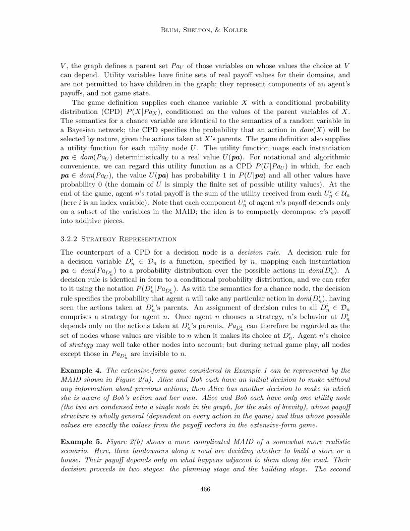
Example 4. The extensive-form game considered in Example 1 can be represented by theMAID shown in Figure 2(a). Alice and Bob each have an initial decision to make withoutany information about previous actions; then Alice has another decision to make in whichshe is aware of Bob’s action and her own. Alice and Bob each have only one utility node(the two are condensed into a single node in the graph, for the sake of brevity), whose payoffstructure is wholly general (dependent on every action in the game) and thus whose possiblevalues are exactly the values from the payoff vectors in the extensive-form game.
Example 5. Figure 2(b) shows a more complicated MAID of a somewhat more realisticscenario. Here, three landowners along a road are deciding whether to build a store or ahouse. Their payoff depends only on what happens adjacent to them along the road. Theirdecision proceeds in two stages: the planning stage and the building stage. The second
466

A Continuation Method for Nash Equilibria in Structured Games
A’
B
A B
A
B1 B2 B3
P3P2P1
C1
E1 E2
C2 C3
L3L2R1 R2
(a) (b)
Figure 2: (a) A simple MAID equivalent to the extensive form game in Figure 1. (b) Atwo-stage road game with three agents.
landowner, for instance, has the two decision variables P2 and B2. He receives a certainpenalty from the utility node C2 if he builds the opposite of what he had planned to build.But after planning, he learns something about what his neighbor to the left has planned.The chance node E1 represents noisy espionage; it transmits the action taken at P1. Afterlearning the value of E1, it may be in the second landowner’s interests to deviate fromhis plan, even if it means incurring the penalty. It is in his interest to start a trend thatdistinguishes him from previous builders but which subsequent builders will follow: the utilitynode L2 rewards him for building the opposite of what was built at B1, and the utility nodeR2 rewards him if the third landowner builds the same thing he does at B3.
Note that this MAID exhibits perfect recall, because the choice made at a planning stageis visible to the agent when it makes its next choice at the building stage.
3.2.3 Payoffs
Under a particular strategy profile σ — that is, a tuple of strategies for all players — alldecision nodes have CPDs specified. Since chance and utility nodes are endowed with CPDsalready, the MAID therefore induces a fully-specified Bayesian network Bσ with variablesV = X ∪ D ∪ U and the same directed graph as the MAID. By the chain rule for Bayesiannetworks, Bσ induces a joint probability distribution Pσ over all the variables in V byPσ(V) =
∏V ∈V P (V |PaV ), with CPDs for chance and utility variables given by the MAID
definition and CPDs for decision variables given by σ. For a game G represented as aMAID, the expected payoff that agent n receives under σ is the expectation of n’s utilitynode values with respect to this distribution:
Gn(σ) =∑
U in∈Un
EPσ [U in]
=∑
U in∈Un
∑u∈dom(U i
n)
u · Pσ(u).
467

Blum, Shelton, & Koller
We show in Section 7 that this and other related expectations can be calculated efficientlyusing Bayesian network inference algorithms, giving a substantial performance increase overthe calculation of payoffs in the extensive-form game.
3.2.4 Extensive Form Strategy Representations in MAIDs
A MAID provides a compact definition of an extensive-form game. We note that, althoughthis correspondence between MAIDs and extensive form games provides some intuitionabout MAIDs, the details of the mapping are not relevant to the remainder of the discussion.We therefore briefly review this construction, referring to the work of Koller and Milch(2001) for details.
The game tree associated with a MAID is a full, balanced tree, with each path corre-sponding to a complete assignment of the chance and decision nodes in the network. Eachnode in the tree corresponds either to a chance node or to a decision node of one of theplayers, with an outgoing branch for each possible action at that node. All nodes at thesame depth in the tree correspond to the same MAID node. We assume that the nodesalong a path in the tree are ordered consistently with the ordering implied by the directededges in the MAID, so that if a MAID node X is a parent of a MAID node Y , the treebranches on X before it branches on Y . The information sets for tree nodes associatedwith a decision node Di
n correspond to assignments to the parents PaDin: all tree nodes
corresponding to Din with the same assignment to PaDi
nare in a single information set.
We note that, by construction, the assignment to PaDin
was determined earlier in the tree,and so the partition to information sets is well-defined. For example, the simple MAID inFigure 2(a) expands into the much larger game tree that we saw earlier in Figure 1.
Translating in the opposite direction, from extensive-form games to MAIDs, is notalways as natural. If the game tree is unbalanced, then we cannot simply reverse the aboveprocess. However, with care, it is possible to construct a MAID that is no larger than agiven extensive-form game, and that may be exponentially smaller in the number of agents.The details are fairly technical, and we omit them here in the interest of brevity.
Despite the fact that a MAID will typically be much more compact than the equivalentextensive-form game, the strategy representations of the two turn out to be equivalent andof equal size. A decision rule for a decision variable Di
n assigns a distribution over actions toeach joint assignment to PaDi
n, just as a behavior strategy assigns a distribution over actions
to an information set in an extensive form game — as discussed above, each assignment tothe parents of Di
n is an information set. A strategy profile for a MAID — a set of decisionrules for every decision variable — is therefore equivalent to a set of behavior strategies forevery information set, which is simply a behavior profile.
If we make the assumption of perfect recall, then, since MAID strategies are simplybehavior strategies, we can represent them in sequence form. Perfect recall requires thatno agent forget anything that it has learned over the course of the game. In the MAIDformalism, the perfect recall assumption is equivalent to the following constraint: if agentn has two decision nodes Di
n and Djn, with the second occurring after the first, then all
parents of Din (the information n is aware of in making decision Di
n) and Din itself must be
parents of Djn. This implies that agent n’s final decision node Dd
n has, as parents, all of n’sprevious decision nodes and their parents. Then a joint assignment to Dd
n ∪PaDdn
precisely
468

A Continuation Method for Nash Equilibria in Structured Games
determines agent n’s sequence of information sets and actions leading to an outcome of thegame — the agent-n history of the outcome.
The realization probability for a particular sequence is computed by multiplying allbehavior strategy probabilities for actions in that sequence. In MAIDs, a sequence cor-responds to a joint assignment to Dd
n ∪ PaDdn, and the behavior strategy probabilities for
this sequence are entries consistent with this assignment in the decision rules for agent n.We can therefore derive all of agent n’s realization probabilities at once by multiplyingtogether, as conditional probability distributions, the decision rules of each of agent n’s de-cision nodes in the sequence — when multiplying conditional probability distributions, onlythose entries whose assignments are consistent with each other are multiplied. Conversely,given a realization plan, we can derive the behavior strategies and hence the decision rulesaccording to the method outlined for extensive-form games.
In the simple MAID example in Figure 2(a), the terminal sequences are the same asin the equivalent extensive-form game. In the road example in Figure 2(b), agent 2 has 8terminal sequences; one for each joint assignment to his final decision node (B2) and itsparents (E1 and P2). Their associated realization probabilities are given by multiplying thedecision rules at P2 and at B2.
4. Computational Complexity
When developing algorithms to compute equilibria efficiently, the question naturally arisesof how well one can expect these algorithms to perform. The complexity of computingNash equilibria has been studied for some time. Gilboa and Zemel (1989) first showedthat it is NP-hard to find more than one Nash equilibrium in a normal-form game, andConitzer and Sandholm (2003) recently utilized a simpler reduction to arrive at this resultand several others in the same vein. Other recent hardness results pertain to restrictedsubclasses of normal-form games (e.g., Chu & Halpern, 2001; Codenotti & Stefankovic,2005). However, these results apply only to 2-agent normal-form games. While it is truethat proving a certain subclass of a class of problems to be NP-hard also proves the entireclass to be NP-hard (because NP-hardness is a measure of worst-case complexity), such aproof might tell us very little about the complexity of problems outside the subclass. Thisissue is particularly apparent in the problem of computing equilibria, because games cangrow along two distinct axes: the number of agents, and the number of actions per agent.The hardness results of Conitzer and Sandholm (2003) apply only as the number of actionsper agent increases. Because 2-agent normal-form games are (fully connected) graphicalgames, these results apply to graphical games.
However, we are more interested in the hardness of graphical games as the numberof agents increases, rather than the number of actions per agent. It is graphical gameswith large numbers of agents that capture the most structure — these are the games forwhich the graphical game representation was designed. In order to prove results about theasymptotic hardness of computing equilibria along this more interesting (in this setting)axis of representation size, we require a different reduction. Our proof, like a number ofprevious hardness proofs for games (e.g., Chu & Halpern, 2001; Conitzer & Sandholm, 2003;Codenotti & Stefankovic, 2005), reduces 3SAT to equilibrium computation. However, inthese previous proofs, variables in 3SAT instances are mapped to actions (or sets of actions)
469

Blum, Shelton, & Koller
in a game with only 2 players, whereas in our reduction they are mapped to agents. Althoughdiffering in approach, our reduction is very much in the spirit of the reduction appearing inthe work of Conitzer and Sandholm (2003), and many of the corollaries of their main resultalso follow from ours (in a form adapted to graphical games).
Theorem 6. For any constant d ≥ 5, and k ≥ 2, the problem of deciding whether agraphical game with a family size at most d and at most k actions per player has more thanone Nash equilibrium is NP-hard.
Proof. Deferred to Appendix B.
In our reduction, all games that have more than one equilibria have at least one purestrategy equilibrium. This immediately gives us
Corollary 7. It is NP-hard to determine whether a graphical game has more than one Nashequilibrium in discretized strategies with even the coarsest possible granularity.
Finally, because graphical games can be represented as (trivial) MAIDs, in which eachagent has only a single parentless decision node and a single utility node, and each agent’sutility node has, as parents, the decision nodes of the graphical game family of that agent,we obtain the following corollary.
Corollary 8. It is NP-hard to determine whether a MAID with constant family size at least6 has more than one Nash equilibrium.
5. Continuation Methods
Continuation methods form the basis of our algorithms for solving each of these struc-tured game representations. We begin with a high-level overview of continuation methods,referring the reader to the work of Watson (2000) for a more detailed discussion.
Continuation methods work by solving a simpler perturbed problem and then tracingthe solution as the magnitude of the perturbation decreases, converging to a solution forthe original problem. More precisely, let λ be a scalar parameterizing a continuum ofperturbed problems. When λ = 0, the perturbed problem is the original one; when λ = 1,the perturbed problem is one for which the solution is known. Let w represent the vectorof real values of the solution. For any perturbed problem defined by λ, we characterizesolutions by the equation F (w, λ) = 0, where F is a real-valued vector function of the samedimension as w (so that 0 is a vector of zeros). The function F is such that w is a solutionto the problem perturbed by λ if and only if F (w, λ) = 0.
The continuation method traces solutions along the level set of solution pairs (w, λ)satisfying F (w, λ) = 0. Specifically, if we have a solution pair (w, λ), we would like to tracethat solution to a nearby solution. Differential changes to w and λ must cancel out so thatF remains equal to 0.
If (w, λ) changes in the direction of a unit vector u, then F will change in the direction∇F · u, where ∇F is the Jacobian of F (which can also be written
[∇wF ∇λF
]). We
want to find a direction u such that F remains unchanged, i.e., equal to 0. Thus, we needto solve the matrix equation [
∇wF ∇λF] [
dwdλ
]= 0 . (3)
470

A Continuation Method for Nash Equilibria in Structured Games
Equivalently, changes dw and dλ along the path must obey ∇wF ·dw = −∇λ F ·dλ. Ratherthan inverting the matrix∇wF in solving this equation, we use the adjoint adj(∇wF ), whichis still defined when ∇wF has a null space of rank 1. The adjoint is the matrix of cofactors:the element at (i, j) is (−1)i+j times the determinant of the sub-matrix in which row i andcolumn j have been removed. When the inverse is defined, adj(∇wF ) = det(∇wF )[∇wF ]−1.In practice, we therefore set dw = −adj(∇wF ) · ∇λF and dλ = det(∇wF ). If the Jacobian[∇wF ∇λF ] has a null-space of rank 1 everywhere, the curve is uniquely defined.
The function F should be constructed so that the curve starting at λ = 1 is guaranteedto cross λ = 0, at which point the corresponding value of w is a solution to the originalproblem. A continuation method begins at the known solution for λ = 1 . The null-space ofthe Jacobian ∇F at a current solution (w, λ) defines a direction, along which the solutionis moved by a small amount. The Jacobian is then recalculated and the process repeats,tracing the curve until λ = 0. The cost of each step in this computation is at least cubic inthe size of w, due to the required matrix operations. However, the Jacobian itself may ingeneral be much more difficult to compute. Watson (2000) provides some simple examplesof continuation methods.
6. Continuation Methods for Games
We now review the work of GW on applying the continuation method to the task of find-ing equilibria in games. They provide continuation methods for both normal-form andextensive-form games. These algorithms form the basis for our extension to structuredgames, described in the next section. The continuation methods perturb the game by giv-ing agents fixed bonuses, scaled by λ, for each of their actions, independently of whateverelse happens in the game. If the bonuses are large enough (and unique), they dominate theoriginal game structure, and the agents need not consider their opponents’ actions. Thereis thus a unique pure-strategy equilibrium easily determined by the bonuses at λ = 1. Thecontinuation method can then be used to follow a path in the space of λ and equilibriumprofiles for the resulting perturbed game, decreasing λ until it is zero; at this point, thecorresponding strategy profile is an equilibrium of the original game.
6.1 Continuation Method for Normal-Form Games
We now make this intuition more precise, beginning with normal-form games.
6.1.1 Perturbations
A perturbation vector b is a vector of m values chosen at random, one for each action in thegame. The bonus ba is given to the agent n owning action a for playing a, independently ofwhatever else happens in the game. Applying this perturbation to a target game G givesus a new game, which we denote G ⊕ b, in which, for each a ∈ An, and for any t ∈ A−n,(G ⊕ b)n(a, t) = Gn(a, t) + ba. If b is made sufficiently large, then G ⊕ b has a uniqueequilibrium, in which each agent plays the pure strategy a for which ba is maximal.
471

Blum, Shelton, & Koller
6.1.2 Characterization of Equilibria
In order to apply Equation (3), we need to characterize the equilibria of perturbed games asthe zeros of a function F . Using a structure theorem of Kohlberg and Mertens (1986), GWshow that the continuation method path deriving from their equilibrium characterizationleads to convergence for all perturbation vectors except those in a set of measure zero. Wepresent only the equilibrium characterization here; proofs of the characterization and of themethod’s convergence are given by Govindan and Wilson (2003).
We first define an auxiliary vector function V G(σ), indexed by actions, of the payoffs toeach agent for deviating from σ to play a single action. We call V G the deviation function.The element V G
a (σ) corresponding to a single action a, owned by an agent n, is the payoffto agent n when it deviates from the mixed strategy profile σ by playing the pure strategyfor action a:
V Ga (σ) =
∑t∈A−n
Gn(a, t)∏
k∈N\{n}
σtk . (4)
It can also be viewed as the component of agent n’s payoff that it derives from action a,under the strategy profile σ. Since bonuses are given to actions independently of σ, theeffect of bonuses on V G is independent of σ. V G
a measures the payoff for deviating andplaying a, and bonuses are given for precisely this deviation, so V G⊕b(σ) = V G(σ) + b.
We also utilize the retraction operator R : IRm → Σ defined by Gul, Pearce, and Sta-chetti (1993), which maps an arbitrary m-vector w to the point in the space Σ of mixedstrategies which is nearest to w in Euclidean distance. Given this operator, the equilibriumcharacterization is as follows.
Lemma 9. (Gul et al., 1993) If σ is a strategy profile of G, then σ = R(V G(σ) + σ) iff σis an equilibrium.
Although we omit the proof, we will give some intuition for why this result is true.Suppose σ is a fully-mixed equilibrium; that is, every action has non-zero probability. Fora single agent n, V G
a (σ) must be the same for all actions a ∈ An, because n should not haveany incentive to deviate and play a single one of them. Let Vn be the vector of entries inV G(σ) corresponding to actions of n, and let σn be defined similarly. Vn is a scalar multipleof 1, the all-ones vector, and the simplex Σn of n’s mixed strategies is defined by 1T x = 1,so Vn is orthogonal to Σn. V G(σ) is therefore orthogonal to Σ, so retracting σ+V G(σ) ontoΣ gives precisely σ. In the reverse direction, if σ is a fully-mixed strategy profile satisfyingσ = R(V G(σ) + σ), then V G(σ) must be orthogonal to the polytope of mixed strategies.Then, for each agent, every pure strategy has the same payoff. Therefore, σ is in fact anequilibrium. A little more care must be taken when dealing with actions not in the support.We refer to Gul et al. (1993) for the details.
According to Lemma 9, we can define an equilibrium as a solution to the equationσ = R(σ + V G(σ)). On the other hand, if σ = R(w) for some w ∈ IRm, we have theequivalent condition that w = R(w) + V G(R(w)); σ is an equilibrium iff this conditionis satisfied, as can easily be verified. We can therefore search for a point w ∈ IRm whichsatisfies this equality, in which case R(w) is guaranteed to be an equilibrium.
The form of our continuation equation is then
F (w, λ) = w −R(w)−(V G (R (w)) + λb
). (5)
472

A Continuation Method for Nash Equilibria in Structured Games
We have that V G +λb is the deviation function for the perturbed game G⊕λb, so F (w, λ)is zero if and only if R(w) is an equilibrium of G⊕ λb. At λ = 0 the game is unperturbed,so F (w, 0) = 0 iff R(w) is an equilibrium of G.
6.1.3 Computation
The expensive step in the continuation method is the calculation of the Jacobian ∇wF ,required for the computation that maintains the constraint of Equation (3). Here, we havethat ∇wF = I − (I +∇V G)∇R, where I is the m ×m identity matrix. The hard part isthe calculation of ∇V G. For pure strategies a ∈ An and a′ ∈ An′ , for n′ 6= n, the valueat location (a, a′) in ∇V G(σ) is equal to the expected payoff to agent n when it plays thepure strategy a, agent n′ plays the pure strategy a′, and all other agents act according tothe strategy profile σ:
∇V Ga,a′(σ) =
∂
∂σa′
∑t∈A−n
Gn(a, t)∏
k∈N\{n}
σtk
=∑
t∈A−n,n′
Gn(a, a′, t)∏
k∈N\{n,n′}
σtk. (6)
If both a ∈ An and a′ ∈ An, ∇V Ga,a′(σ) = 0.
Computing Equation (6) requires a large number of multiplications; the sum is over thespace A−n,n′ =
∏k∈N\{n,n′} Ai, which is exponentially large in the number of agents.
6.2 Continuation Method for Extensive-Form Games
The same method applies to extensive-form games, using the sequence form strategy rep-resentation.
6.2.1 Perturbations
As with normal-form games, the game is perturbed by the bonus vector b. Agent n owningsequence h is paid an additional bonus bh for playing h, independently of whatever elsehappens in the game. Applying this perturbation gives us a new game G⊕ b in which, foreach z ∈ Z, (G⊕ b)n(z) = Gn(z) + bHn(z).
If the bonuses are large enough and unique, GW show that once again the perturbedgame has a unique pure-strategy equilibrium (one in which all realization probabilities are0 or 1). However, calculating it is not as simple as in the case of normal-form games.Behavior strategies must be calculated from the leaves upward by a recursive procedure, inwhich at each step the agent who owns the node in question chooses the action that resultsin the sequence with the largest bonus. Since all actions below it have been recursivelydetermined, each action at the node in question determines an outcome. The realizationplans can be derived from this behavior profile by the method outlined in Section 2.2.1.
473

Blum, Shelton, & Koller
6.2.2 Characterization of Equilibria
Once more, we first define a vector function capturing the benefit of deviating from a givenstrategy profile, indexed by sequences:
V Gh (σ) =
∑z∈Zh
Gn(z)∏
k∈N\{n}
σk(z), (7)
where Zh is the set of leaves that are consistent with the sequence h. The interpretation ofV G is not as natural as in the case of normal-form games, as it is not possible for an agentto play one sequence to the exclusion of all others; its possible actions will be partiallydetermined by the actions of other agents. In this case, V G
h (σ) can be regarded as theportion of its payoff that agent n receives for playing sequence h, unscaled by agent n’s ownprobability of playing that sequence. As with normal-form games, the vector of bonuses isadded directly to V G, so V G⊕b = V G + b.
The retraction operator R for realization plans is defined in the same way as for normal-form strategies: it takes a general vector and projects it onto the nearest point in the validregion of realization plans. The constraints defining this space are linear, as discussed inSection 2.2.1 . We can therefore express them as a constraint matrix C with Cσ = 0 forall valid profiles σ. In addition, all probabilities must be greater than or equal to zero. Tocalculate w, we must find a σ minimizing (w−σ)T (w−σ), the (squared) Euclidean distancebetween w and σ, subject to Cσ = 0 and σ ≥ 0. This is a quadratic program (QP), whichcan be solved efficiently using standard methods. The Jacobian of the retraction is easilycomputable from the set of active constraints.
The equilibrium characterization for realization plans is now surprisingly similar tothat of mixed strategies in normal-form games; GW show that, as before, equilibria arecharacterized by σ = R(σ + V G(σ)), where now R is the retraction for sequence form andV G is the deviation function. The continuation equation F takes exactly the same form aswell.
6.2.3 Computation
The key property of the reduced sequence-form strategy representation is that the devi-ation function is a multi-linear function of the extensive-form parameters, as shown inEquation (7). The elements of the Jacobian ∇V G thus also have the same general struc-ture. In particular, the element corresponding to sequence h for agent n and sequence h′
for agent n′ is
∇V Gh,h′(σ) =
∂
∂σh′
∑z∈Zh
Gn(z)∏
k∈N\{n}
σk(z)
=∑
z∈Zh,h′
Gn(z)∏
k∈N\{n,n′}
σk(z) (8)
where Zh,h′ is the set of leaves that are consistent with the sequences h (for agent n) andh′ (for agent n′). Zh,h′ is the empty set (and hence ∇V G = 0) if h and h′ are incompatible.Equation (8) is precisely analogous to Equation (6) for normal-form games. We have a sumover outcomes of the utility of the outcome multiplied by the strategy probabilities for all
474

A Continuation Method for Nash Equilibria in Structured Games
σ
λ
1
2
3
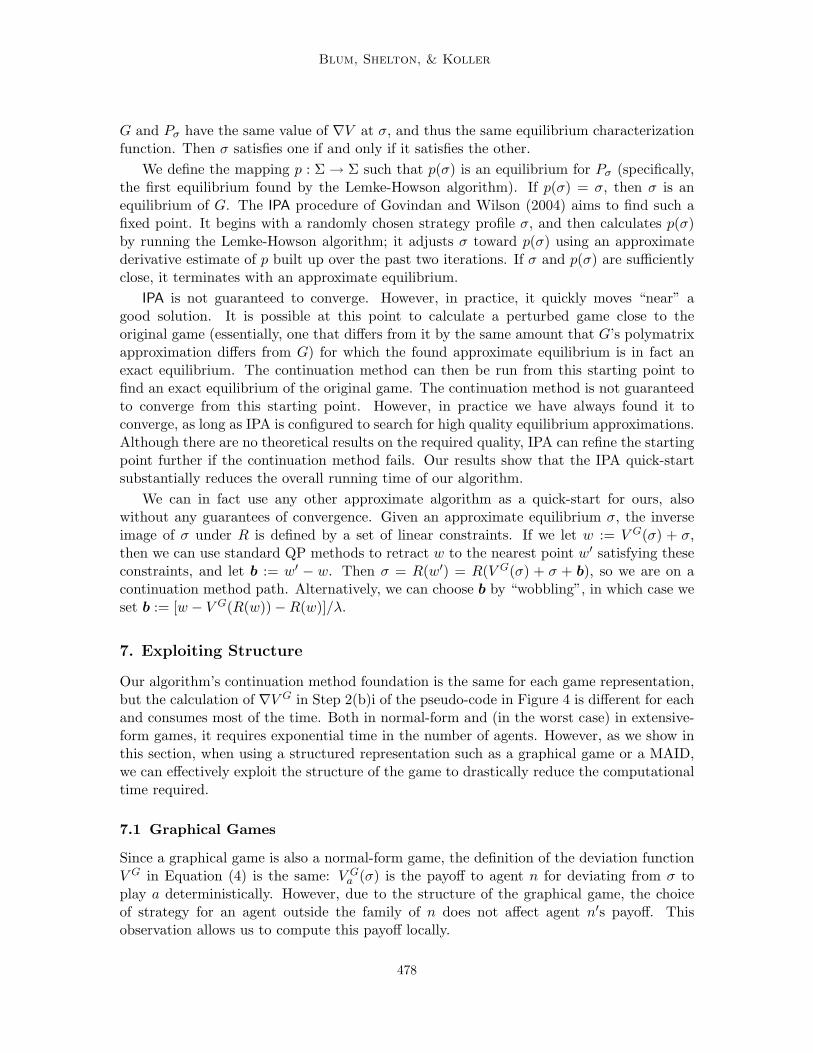
Figure 3: An abstract diagram of the path. The horizontal axis represents λ and the verticalaxis represents the space of strategy profiles (actually multidimensional). Thealgorithm starts on the right at λ = 1 and follows the dynamical system untilλ = 0 at point 1, where it has found an equilibrium of the original game. It cancontinue to trace the path and find the equilibria labeled 2 and 3.
other agents. Note that this sum is over the leaves of the tree, which may be exponentiallynumerous in the number of agents.
One additional subtlety, which must be addressed by any method for equilibrium com-putation in extensive-form games, relates to zero-probability actions. Such actions inducea probability of zero for entire trajectories in the tree, possibly leading to equilibria basedon unrealizable threats. Additionally, for information sets that occur with zero probability,agents can behave arbitrarily without disturbing the equilibrium criterion, resulting in a con-tinuum of equilibria and a possible bifurcation in the continuation path. This prevents ourmethods from converging. We therefore constrain all realization probabilities to be greaterthan or equal to ε for some small ε > 0. This is, in fact, a requirement for GW’s equilibriumcharacterization to hold. The algorithm thus looks for an ε-perfect equilibrium (Fudenberg& Tirole, 1991): a strategy profile σ in which each component is constrained by σs ≥ ε, andeach agent’s strategy is a best response among those satisfying the constraint. Note thatthis is entirely different from an ε-equilibrium. An ε-perfect equilibrium always exists, aslong as ε is not so large as to make the set of legal strategies empty. An ε-perfect equilib-rium can be interpreted as an equilibrium in a perturbed game in which agents have a smallprobability of choosing an unintended action. A limit of ε-perfect equilibria as ε approaches0 is a perfect equilibrium (Fudenberg & Tirole, 1991): a refinement of the basic notion ofa Nash equilibrium. As ε approaches 0, the equilibria found by GW’s algorithm thereforeconverge to an exact perfect equilibrium, by continuity of the variation in the continuationmethod path. Then for ε small enough, there is a perfect equilibrium in the vicinity of thefound ε-perfect equilibrium, which can easily be found with local search.
475

Blum, Shelton, & Koller
6.3 Path Properties
In the case of normal-form games, GW show, using the structure theorem of Kohlberg andMertens (1986), that the path of the algorithm is a one-manifold without boundary withprobability one over all choices for b. They provide an analogous structure theorem thatguarantees the same property for extensive-form games. Figure 3(a) shows an abstractrepresentation of the path followed by the continuation method. GW show that the pathmust cross the λ = 0 hyperplane at least once, yielding an equilibrium. In fact, the pathmay cross multiple times, yielding many equilibria in a single run. As the path musteventually continue to the λ = −∞ side, it will find an odd number of equilibria when runto completion.
In both normal-form and extensive-form games, the path is piece-wise polynomial, witheach piece corresponding to a different support set of the strategy profile. These pieces arecalled support cells. The path is not smooth at cell boundaries due to discontinuities in theJacobian of the retraction operator, and hence in ∇wF , when the support changes. Caremust be taken to step up to these boundaries exactly when following the path; at this point,the Jacobian for the new support can be calculated and the path can be traced into thenew support cell.
In the case of two agents, the path is piece-wise linear and, rather than taking steps, thealgorithm can jump from corner to corner along the path. When this algorithm is applied toa two-agent game and a particular bonus vector is used (in which only a single entry is non-zero), the steps from support cell to support cell that the algorithm takes are identical tothe pivots of the Lemke-Howson algorithm (Lemke & Howson, 1964) for two-agent general-sum games, and the two algorithms find precisely the same set of solutions (Govindan &Wilson, 2002). Thus, the continuation method is a strict generalization of the Lemke-Howson algorithm that allows different perturbation rays and games of more than twoagents.
This process is described in more detail in the pseudo-code for the algorithm, presentedin Figure 4.
6.4 Computational Issues
Guarantees of convergence apply only as long as we stay on the path defined by the dy-namical system of the continuation method. However, for computational purposes, discretesteps must be taken. As a result, error inevitably accumulates as the path is traced, so thatF becomes slightly non-zero. GW use several simple techniques to combat this problem.We adopt their techniques, and introduce one of our own: we employ an adaptive stepsize, taking smaller steps when error accumulates quickly and larger ones when it does not.When F is nearly linear (as it is, for example, when very few actions are in the support ofthe current strategy profile), this technique speeds computation significantly.
GW use two different techniques to remove error once it has accumulated. Suppose weare at a point (w, λ) and we wish to minimize the magnitude of F (w, λ) = w−V G(R(w))+λb+R(w). There are two values we might change: w, or λb. We can change the first withoutaffecting the guarantee of convergence, so every few steps we run a local Newton methodsearch for a w minimizing |F (w, λ)|. If this search does not decrease error sufficiently, thenwe perform what GW call a “wobble”: we change the perturbation vector (“wobble” the
476

A Continuation Method for Nash Equilibria in Structured Games
continuation path) to make the current solution consistent. If we set b = [w−V G(R(w))−R(w)]/λ, the equilibrium characterization equation is immediately satisfied. Changing theperturbation vector invalidates any theoretical guarantees of convergence. However, it isnonetheless an attractive option because it immediately reduces error to zero. Both thelocal Newton method and the “wobbles” are described in more detail by Govindan andWilson (2003).
These techniques can potentially send the algorithm into a cycle, and in practice theyoccasionally do. However, they are necessary for keeping the algorithm on the path. If thealgorithm cycles, random restarts and a decrease in step size can improve convergence. Moresophisticated path-following algorithms might also be used, and in general could improvethe success rate and execution time of the algorithm.
6.5 Iterated Polymatrix Approximation
Because perturbed games may themselves have a large number of equilibria, and the pathmay wind back and forth through any number of them, the continuation algorithm cantake a while to trace its way back to a solution to the original game. We can speed up thealgorithm using an initialization procedure based on the iterated polymatrix approximation(IPA) algorithm of GW. A polymatrix game is a normal-form game in which the payoffs toan agent n are equal to the sum of the payoffs from a set of two-agent games, each involvingn and another agent. Because polymatrix games are a linear combination of two-agentnormal-form games, they reduce to a linear complementarity problem and can be solvedquickly using the Lemke-Howson algorithm (Lemke & Howson, 1964).
For each agent n ∈ N in a polymatrix game, the payoff array is a matrix Bn indexedby the actions of agent n and of each other agent; for actions a ∈ An and a′ ∈ An′ , Bn
a,a′
is the payoff n receives for playing a in its game with agent n′, when n′ plays a′. Agentn’s total payoff is the sum of the payoffs it receives from its games with each other agent,∑
n′ 6=n
∑a∈An,a′∈An′
σaσa′Bna,a′ . Given a normal-form game G and a strategy profile σ, we
can construct the polymatrix game Pσ whose payoff function has the same Jacobian at σas G’s by setting
Bna,a′ = ∇V G
a,a′(σ) . (9)
The game Pσ is a linearization of G around σ: its Jacobian is the same everywhere. GWshow that σ is an equilibrium of G if and only if it is an equilibrium of Pσ. This followsfrom the equation V G(σ) = ∇V G(σ) · σ/(|N | − 1), which holds for all σ. To see why itholds, consider the single element indexed by a ∈ An:
(∇V G(σ) · σ)a =∑
n′∈N\{n}
∑a′∈An′
σa′∑
t∈A−n,−n′
Gn(a, a′, t)∏
k∈N\{n,n′}
σtk
=∑
n′∈N\{n}
∑t∈A−n
Gn(a, t)∏
k∈N\{n}
σtk
= (|N | − 1)V G(σ)a.
The equilibrium characterization equation can therefore be written
σ = R(σ +∇V G (σ) · σ (|N | − 1)
).
477
Blum, Shelton, & Koller
G and Pσ have the same value of ∇V at σ, and thus the same equilibrium characterizationfunction. Then σ satisfies one if and only if it satisfies the other.
We define the mapping p : Σ → Σ such that p(σ) is an equilibrium for Pσ (specifically,the first equilibrium found by the Lemke-Howson algorithm). If p(σ) = σ, then σ is anequilibrium of G. The IPA procedure of Govindan and Wilson (2004) aims to find such afixed point. It begins with a randomly chosen strategy profile σ, and then calculates p(σ)by running the Lemke-Howson algorithm; it adjusts σ toward p(σ) using an approximatederivative estimate of p built up over the past two iterations. If σ and p(σ) are sufficientlyclose, it terminates with an approximate equilibrium.
IPA is not guaranteed to converge. However, in practice, it quickly moves “near” agood solution. It is possible at this point to calculate a perturbed game close to theoriginal game (essentially, one that differs from it by the same amount that G’s polymatrixapproximation differs from G) for which the found approximate equilibrium is in fact anexact equilibrium. The continuation method can then be run from this starting point tofind an exact equilibrium of the original game. The continuation method is not guaranteedto converge from this starting point. However, in practice we have always found it toconverge, as long as IPA is configured to search for high quality equilibrium approximations.Although there are no theoretical results on the required quality, IPA can refine the startingpoint further if the continuation method fails. Our results show that the IPA quick-startsubstantially reduces the overall running time of our algorithm.
We can in fact use any other approximate algorithm as a quick-start for ours, alsowithout any guarantees of convergence. Given an approximate equilibrium σ, the inverseimage of σ under R is defined by a set of linear constraints. If we let w := V G(σ) + σ,then we can use standard QP methods to retract w to the nearest point w′ satisfying theseconstraints, and let b := w′ − w. Then σ = R(w′) = R(V G(σ) + σ + b), so we are on acontinuation method path. Alternatively, we can choose b by “wobbling”, in which case weset b := [w − V G(R(w))−R(w)]/λ.
7. Exploiting Structure
Our algorithm’s continuation method foundation is the same for each game representation,but the calculation of ∇V G in Step 2(b)i of the pseudo-code in Figure 4 is different for eachand consumes most of the time. Both in normal-form and (in the worst case) in extensive-form games, it requires exponential time in the number of agents. However, as we show inthis section, when using a structured representation such as a graphical game or a MAID,we can effectively exploit the structure of the game to drastically reduce the computationaltime required.
7.1 Graphical Games
Since a graphical game is also a normal-form game, the definition of the deviation functionV G in Equation (4) is the same: V G
a (σ) is the payoff to agent n for deviating from σ toplay a deterministically. However, due to the structure of the graphical game, the choiceof strategy for an agent outside the family of n does not affect agent n′s payoff. Thisobservation allows us to compute this payoff locally.
478

A Continuation Method for Nash Equilibria in Structured Games
For an input game G:
1. Set λ = 1, choose initial b and σ either by a quick-start procedure (e.g., IPA) or by randomizing. Setw = V G(σ) + λb + σ.
2. While λ is greater than some (negative) threshold (i.e., there is still a good chance of picking upanother equilibrium):
(a) Initialize for the current support cell: set the steps counter to the number of steps we will takein crossing the cell, depending on the current amount of error. If F is linear or nearly linear (if,for example, the strategy profile is nearly pure, or there are only 2 agents), set steps = 1 so wewill cross the entire cell.
(b) While steps ≥ 1:
i. Compute ∇V G(σ).
ii. Set ∇wF (w, λ) = I − (∇V G(σ) + I)∇R(w) (we already know ∇λF = −b). Set dw =adj(∇wF ) · b and dλ = det(∇wF ). These satisfy Equation (3).
iii. Set δ equal to the distance we’d have to go in the direction of dw to reach the next supportboundary. We will scale dw and dλ by δ/steps.
iv. If λ will change signs in the course of the step, record an equilibrium at the point whereit is 0.
v. Set w := w + dw(δ/steps) and λ := λ + dλ(δ/steps).
vi. If sufficient error has accumulated, use the local Newton method to find a w minimizing|F (w, λ)|. If this does not reduce error enough, increase steps, thereby decreasing stepsize. If we have already increased steps, perform a “wobble” and reassign b.
vii. Set steps := steps− 1.
Figure 4: Pseudo-code for the cont algorithm.
7.1.1 The Jacobian for Graphical Games
We begin with the definition of V G for normal-form games (modified slightly to accountfor the local payoff arrays). Recall that Af
−n is the set of action profiles of agents in Famn
other than n, and let A−Famn be the set of action profiles of agents not in Famn. Thenwe can divide a sum over full action profiles between these two sets, switching from thenormal-form version of Gn to the graphical game version of Gn, as follows:
V Ga (σ) =
∑t∈A−n
Gn(a, t)∏
k∈N\{n}
σtk
=∑
u∈Af−n
Gn(a,u)∏
k∈Famn\{n}
σuk
∑v∈A−Famn
∏j∈N\Famn
σvj . (10)
Note that the latter sum and product simply sum out a probability distribution, and henceare always equal to 1 due to the constraints on σ. They can thus be eliminated withoutchanging the value V G takes on valid strategy profiles. However, their partial derivativeswith respect to strategies of agents not in Famn are non-zero, so they enter into the com-putation of ∇V G.
Suppose we wish to compute a row in the Jacobian matrix corresponding to action a ofagent n. We must compute the entries for each action a′ of each agent n′ ∈ N . In the trivialcase where n′ = n then ∇V G
a,a′ = 0, since σa does not appear anywhere in the expressionfor V G
a (σ). We next compute the entries for each action a′ of each other agent n′ ∈ Famn.
479

Blum, Shelton, & Koller
In this case,
∇V Ga,a′(σ) =
∂
∂σa′
∑u∈Af
−n
Gn(a,u)∏
k∈Famn\{n}
σuk
∑v∈A−Famn
∏j∈N\Famn
σvj (11)
=∑
u∈Af−n
Gn(a,u)∂
∂σa′
∏k∈Famn\{n}
σuk· 1
=∑
t∈Af
−n,n′
Gn(a, a′, t)∏
k∈Famn\{n,n′}
σtk, if n′ ∈ Famn . (12)
We next compute the entry for a single action a′ of an agent n′ /∈ Famn. The derivative inEquation (11) takes a different form in this case; the variable in question is in the secondsummation, not the first, so that we have
∇V Ga,a′(σ) =
∂
∂σa′
∑u∈Af
−n
Gn(a,u)∏
k∈Famn\{n}
σuk
∑v∈A−Famn
∏j∈N\Famn
σvj
=∑
u∈Af−n
Gn(a,u)∏
k∈Famn\{n}
σuk
∑v∈A−Famn
∂
∂σa′
∏j∈N\Famn
σvj
=∑
u∈Af−n
Gn(a,u)∏
k∈Famn\{n}
σuk· 1, if n′ 6∈ Famn . (13)
Notice that this calculation does not depend on a′; therefore, it is the same for each actionof each other agent not in Famn. We need not compute any more elements of the row. Wecan copy this value into all other columns of actions belonging to agents not in Famn.
7.1.2 Computational Complexity
Due to graphical game structure, the computation of ∇V G(σ) takes time exponential onlyin the maximal family size of the game, and hence takes time polynomial in the numberof agents if the family size is constant. In particular, our methods lead to the followingtheorem about the complexity of the continuation method for graphical games.
Theorem 10. The time complexity of computing the Jacobian of the deviation function∇V G(σ) for a graphical game is O(fdf |N | + d2|N |2), where f is the maximal family sizeand d is the maximal number of actions per agent.
Proof. Consider a single row in the Jacobian, corresponding to a single action a owned bya single agent n. There are at most d(f − 1) entries in the row for actions owned by othermembers of Famn. For one such action a′, the computation of the Jacobian element ∇V G
a,a′
according to Equation (12) takes time O(df−2). The total cost for all such entries is thereforeO((f −1)df−1). There are then at most d(|N |−f) entries for actions owned by non-family-members. The value of ∇V G
a,a′ for each such a′ is the same. It can be calculated once in timeO(df−1), then copied across the row in time d(|N | − f). All in all, the computational costfor the row is O(fdf−1 + d|N |). There are at most d|N | rows, so the total computationalcost is O(|N |fdf + d2|N |2).
480

A Continuation Method for Nash Equilibria in Structured Games
A’
B
A
B1 B2 B3
P3P2P1
(a) (b)
Figure 5: The strategic relevance graphs for the MAIDs in (a) Figure 2(a) and (b) Fig-ure 2(b).
Each iteration of the algorithm calculates ∇V G(σ) once; we have therefore proved that asingle iteration takes time polynomial in |N | if f is constant (in fact, matrix operations makethe complexity cubic in |N |). However, as for normal-form games, there are no theoreticalresults about how many steps of the continuation method are required for convergence.
7.2 MAIDs
For graphical games, the exploitation of structure was straightforward. We now turn tothe more difficult problem of exploiting structure in MAIDs. We take advantage of twodistinct sets of structural properties. The first, a coarse-grained structural measure knownas strategic relevance (Koller & Milch, 2001), has been used in previous computationalmethods. After decomposing a MAID according to strategic relevance relations, we canexploit finer-grained structure by using the extensive-form continuation method of GWto solve each component’s equivalent extensive-form game. In the next two sections, wedescribe these two kinds of structure.
7.2.1 Strategic Relevance
Intuitively, a decision node Din is strategically relevant to another decision node Dj
n′ if agentn′, in order to optimize its decision rule at Dj
n′ , needs to know agent n’s decision rule atDi
n. The relevance relation induces a directed graph known as the relevance graph, in whichonly decision nodes appear and an edge from node Dj
n′ to node Din is present iff Di
n isstrategically relevant to Dj
n′ . In the event that the relevance graph is acyclic, the decisionrules can be optimized sequentially in any reverse topological order; when all the childrenof a node Di
n have had their decision rules set, the decision rule at Din can be optimized
without regard for any other nodes.When cycles exist in the relevance graph, however, further steps must be taken. Within
a strongly connected component (SCC), a set of nodes for which a directed path between anytwo nodes exists in the relevance graph, decision rules cannot be optimized sequentially—in any linear ordering of the nodes in the SCC, some node must be optimized before one
481

Blum, Shelton, & Koller
of its children, which is impossible. Koller and Milch (2001) show that a MAID can bedecomposed into SCCs, which can then be solved individually.
For example, the relevance graph for the MAID in Figure 2(a), shown in Figure 5(a),has one SCC consisting of A and B, and another consisting of A′. In this MAID, we wouldfirst optimize the decision rule at A′, as the optimal decision rule at A′ does not rely on thedecision rules at A and B — when she makes her decision at A′, Alice already knows theactions taken at A and B, so she does not need to know the decision rules that led to them.Then we would turn A′ into a chance node with CPD specified by the optimized decisionrule and optimize the decision rules at A′ and B. The relevance graph for Figure 2(b),shown in Figure 5(b), forms a single strongly connected component.
The computational method of Koller and Milch (2001) stops at strategic relevance:each SCC is converted into an equivalent extensive-form game and solved using standardmethods. Our algorithm can be viewed as an augmentation of their method: after a MAIDhas been decomposed into SCCs, we can solve each of these SCCs using our methods, takingadvantage of finer-grained MAID structure within them to find equilibria more efficiently.The MAIDs on which we test our algorithms (including the road MAID in Figure 2b) allhave strongly connected relevance graphs, so they cannot be decomposed (see Figure 5band Figure 10).
7.2.2 The Jacobian for MAIDs
A MAID is equivalent to an extensive-form game, so its deviation function V G is the sameone defined in Equation (8). Now, however, we can compute the payoffs that make up theJacobian ∇V G more efficiently. Consider a payoff Gn(z) to agent n for outcome z. Theoutcome z is simply an assignment x to all of the variables in the MAID. The realizationprobability σn(z) is the product of the probabilities for the decisions of agent n in theassignment x, so the product
∏k∈N σk(z) of all realization probabilities is simply the joint
probability of the assignment. The expected payoff agent n will receive under the strategyprofile σ,
∑z∈Z Gn(z)
∏k∈N σk(z), is therefore an expectation of Gn(z). The expectation
is with respect to the distribution Pσ defined by the Bayesian network Bσ whose structureis the same as the MAID, with decision node CPDs determined by σ.
The entries of ∇V G are not strictly expected payoffs, however. Equation (8) can berewritten as
∇V Gh,h′(σ) =
∑z∈Zh,h′
Gn(z)∏
k∈N σk(z)σn(z)σn′(z)
. (14)
The expectation is of the quantity Gn(z)/[σn(z)σn′(z)]. The payoff Gn(z) is the sum of agentn’s utility nodes. Due to linearity of expectation, we can perform the computation separatelyfor each of agent n’s utility nodes, and then simply add up the separate contributions.
We can therefore restrict our attention to computing the contribution of a single utilitynode Un for each agent n. Furthermore, the value of σn(z) depends only on the valuesof the set of nodes Dn consisting of n’s decision nodes and their parents. Thus, insteadof computing the probabilities for all assignments to all variables, we need only computethe marginal joint distribution over Un, Dn, and Dn′ . From this distribution, we cancompute the contribution of Un to the expectation in Equation (14) for every pair of terminalsequences belonging to agents n and n′.
482
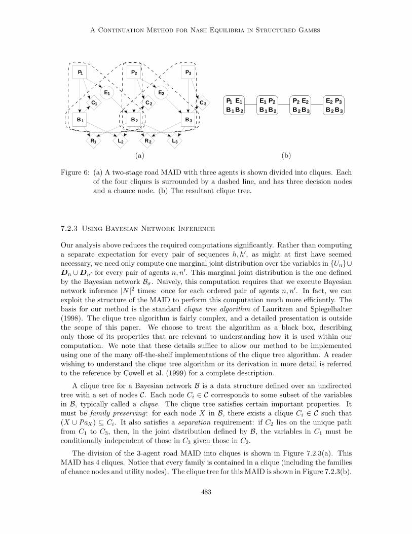
A Continuation Method for Nash Equilibria in Structured Games
B1 B2 B3
P3P2P1
C1
E1 E2
C2 C3
L3L2R1 R2
B1
P1
B2
E1
B1
E1
B2
P2
B2
P2
B3
E2
B2
E2
B3
P3
(a) (b)
Figure 6: (a) A two-stage road MAID with three agents is shown divided into cliques. Eachof the four cliques is surrounded by a dashed line, and has three decision nodesand a chance node. (b) The resultant clique tree.
7.2.3 Using Bayesian Network Inference
Our analysis above reduces the required computations significantly. Rather than computinga separate expectation for every pair of sequences h, h′, as might at first have seemednecessary, we need only compute one marginal joint distribution over the variables in {Un}∪Dn ∪Dn′ for every pair of agents n, n′. This marginal joint distribution is the one definedby the Bayesian network Bσ. Naively, this computation requires that we execute Bayesiannetwork inference |N |2 times: once for each ordered pair of agents n, n′. In fact, we canexploit the structure of the MAID to perform this computation much more efficiently. Thebasis for our method is the standard clique tree algorithm of Lauritzen and Spiegelhalter(1998). The clique tree algorithm is fairly complex, and a detailed presentation is outsidethe scope of this paper. We choose to treat the algorithm as a black box, describingonly those of its properties that are relevant to understanding how it is used within ourcomputation. We note that these details suffice to allow our method to be implementedusing one of the many off-the-shelf implementations of the clique tree algorithm. A readerwishing to understand the clique tree algorithm or its derivation in more detail is referredto the reference by Cowell et al. (1999) for a complete description.
A clique tree for a Bayesian network B is a data structure defined over an undirectedtree with a set of nodes C. Each node Ci ∈ C corresponds to some subset of the variablesin B, typically called a clique. The clique tree satisfies certain important properties. Itmust be family preserving : for each node X in B, there exists a clique Ci ∈ C such that(X ∪ PaX) ⊆ Ci. It also satisfies a separation requirement: if C2 lies on the unique pathfrom C1 to C3, then, in the joint distribution defined by B, the variables in C1 must beconditionally independent of those in C3 given those in C2.
The division of the 3-agent road MAID into cliques is shown in Figure 7.2.3(a). ThisMAID has 4 cliques. Notice that every family is contained in a clique (including the familiesof chance nodes and utility nodes). The clique tree for this MAID is shown in Figure 7.2.3(b).
483

Blum, Shelton, & Koller
Each clique maintains a data structure called a potential, a table with an entry for eachjoint assignment to the variables in the clique. A table of this sort is more generally calleda factor. Inference algorithms typically use two basic operations on factors: factor product,and factor marginalization. If F and G are two factors over the (possibly overlapping) setsof variables X and Y , respectively, then we can define the product FG to be a new factorover X ∪ Y . The entry in FG for a particular assignment to the variables in X ∪ Y is theproduct of the entries in F and G corresponding to the restriction of the assignment to Xand Y , respectively. This notion of multiplication corresponds to the way that conditionalprobability distributions are multiplied. We can also marginalize, or sum, a variable X outof a factor F over X in the same way in which we would sum a variable out of a jointprobability distribution. The result is a factor
∑X F over the variables in X\{X}. The
entry for a particular assignment to the variables in∑
X F is equal to the sum of all entriesin F compatible with that assignment — one for each value of X.
Because a factor has an entry for every joint assignment to its variables, the size ofthe potential for Ci is exponential in |Ci|. The clique tree inference algorithm proceeds bypassing messages, themselves factors, from one clique to another in the tree. The messagesare used to update the potential in the receiving clique by factor multiplication. After aprocess in which messages have been sent in both directions over each edge in the tree, thetree is said to be calibrated ; at this point, the potential of every clique Ci contains preciselythe joint distribution over the variables in Ci according to B (for details, we refer to thereference by Cowell et al., 1999).
We can use the clique tree algorithm to perform inference over Bσ. Consider the finaldecision node for agent n. Due to the perfect recall assumption, all of n’s previous decisionsand all of their parents are also parents of this decision node. The family preservationproperty therefore implies that Dn is fully contained in some clique. It also implies thatthe family of each utility node is contained in a clique. The expectation of Equation (14)thus requires the computation of the joint distribution over three cliques in the tree: the onecontaining PaUn , the one containing Dn, and the one containing Dn′ . We need to computethis joint distribution for every pair of agents n, n′.
The first key insight is that we can reduce this problem to one of computing the joint mar-ginal distribution for all pairs of cliques in the tree. Assume we have computed PB(Ci, Cj)for every pair of cliques Ci, Cj . Now, consider any triple of cliques Ci, Cj , Ck. There are twocases: either one of these cliques is on the path between the other two, or not. In the firstcase, assume without loss of generality that Cj is on the path from Ci to Ck. In this case, bythe separation requirement, we have that PB(Ci, Cj , Ck) = PB(Ci, Cj)PB(Cj , Ck)/PB(Cj).In the second case, there exists a unique clique C∗ that lies on the path between any pairof these cliques. Again, by the separation property, C∗ renders these cliques conditionallyindependent, so we can compute
PB(Ci, Cj , Ck) =∑C∗
PB(Ci, C∗)PB(Cj , C
∗)PB(Ck, C∗)
PB(C∗)2. (15)
Thus, we have reduced the problem to one of computing the marginals over all pairs ofcliques in a calibrated clique-tree. We can use dynamic programming to execute this processefficiently. We construct a table that contains PB(Ci, Cj) for each pair of cliques Ci, Cj . Weconstruct the table in order of length of the path from Ci to Cj . The base case is when Ci and
484

A Continuation Method for Nash Equilibria in Structured Games
Cj are adjacent in the tree. In this case, we have that PB(Ci, Cj) = PB(Ci)PB(Cj)/PB(Ci ∩Cj). The probability expressions in the numerator are simply the clique potentials inthe calibrated tree. The denominator can be obtained by marginalizing either of the twocliques. In fact, this expression is computed as a byproduct of the calibration process, sothe marginalization is not required. For cliques Ci and Cj that are not adjacent, we let Ck
be the node adjacent to Cj on the path from Ci to Cj . The clique Ck is one step closerto Ci, so, by construction, we have already computed P (Ci, Ck). We can now apply theseparation property again:
PB(Ci, Cj) =∑Ck
PB(Ci, Ck)PB(Ck, Cj)PB(Ck)
. (16)
7.2.4 Computational Complexity
Theorem 11. The computation of ∇V G(σ) can be performed in time O(`2d3 + u|N |d4),where ` is the number of cliques in the clique tree for G, d is the size of the largest clique(the number of entries in its potential), |N | is the number of agents, and u is the totalnumber of utility nodes in the game.
Proof. The cost of calibrating the clique tree for Bσ is O(`d). The cost of computingEquation (16) for a single pair of cliques is O(d3), as we must compute a factor over thevariables in three cliques before summing out. We must perform this computation O(`2)times, once for each pair of cliques, for a total cost of O(`2d3). We now compute marginaljoint probabilities over triples of cliques PaU i
n, Dn, Dn′ for every utility node U i
n and everyagent n′ other than n. There are u(|N | − 1) such triples. Computing a factor over thevariables in three cliques may first require computing a factor over the variables in fourcliques, at a cost of O(d4). Given this factor, computing the expected value of the utilitynode takes time O(d3), which does not affect the asymptotic running time. The total cost forcomputing all the marginal joint probabilities and expected utilities is therefore O(u|N |d4),and the total cost for computing ∇V G(σ) is O(`2d3 + u|N |d4).
With this method, we have shown that a single iteration in the continuation methodcan be accomplished in time exponential in the induced width of the graph — the numberof variables in the largest clique in the clique tree. The induced width of the optimal cliquetree — the one with the smallest maximal clique — is called the treewidth of the network.Although finding the optimal clique tree is, itself, an NP-hard problem, good heuristicalgorithms are known (Cowell et al., 1999). In games where interactions between the agentsare highly structured (the road MAID, for example), the size of the largest clique can be aconstant even as the number of agents grows. In this case, the complexity of computing theJacobian grows only quadratically in the number of cliques, and hence also in the numberof agents. Note that the matrix adjoint operation takes time cubic in m, which is at least|N |, so a single step along the path actually has cubic computational cost.
485
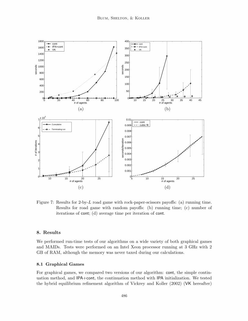
Blum, Shelton, & Koller
0 20 40 60 80 1000
200
400
600
800
1000
1200
1400
1600
1800
# of agents
seco
nds
contIPA+contVK
10 15 20 25 30 35 40 450
50
100
150
200
250
300
350
400
# of agents
seco
nds
cont
IPA+cont
VK
(a) (b)
10 15 20 250
1
2
3
4
5
6
7x 10
4
# of agents
# of
iter
atio
ns
Cumulative
Terminating run
5 10 15 20 250
0.001
0.002
0.003
0.004
0.005
0.006
0.007
0.008
0.009
0.01
# of agents
seco
nds/
itera
tion
contcubic fit
(c) (d)
Figure 7: Results for 2-by-L road game with rock-paper-scissors payoffs: (a) running time.Results for road game with random payoffs: (b) running time; (c) number ofiterations of cont; (d) average time per iteration of cont.
8. Results
We performed run-time tests of our algorithms on a wide variety of both graphical gamesand MAIDs. Tests were performed on an Intel Xeon processor running at 3 GHz with 2GB of RAM, although the memory was never taxed during our calculations.
8.1 Graphical Games
For graphical games, we compared two versions of our algorithm: cont, the simple contin-uation method, and IPA+cont, the continuation method with IPA initialization. We testedthe hybrid equilibrium refinement algorithm of Vickrey and Koller (2002) (VK hereafter)
486

A Continuation Method for Nash Equilibria in Structured Games
5 10 15 20 25 30 35 40 450
100
200
300
400
500
600
# of agents
seco
nds
cont
IPA+cont
VK
5 10 15 20 25 30 35 400
0.5
1
1.5
2
2.5
3
3.5
4
4.5
5x 10
4
# of agents
# of
iter
atio
ns
Cumulative
Terminating run
(a) (b)
5 10 15 20 25 30 350
50
100
150
200
250
# of agents
seco
nds
cont
IPA+cont
VK
10 15 20 250
1
2
3
4
5
6x 10
4
# of agents
# of
iter
atio
nsCumulative
Terminating run
(c) (d)
Figure 8: Results for ring game with random payoffs: (a) running time; (b) number ofiterations of cont. Results for L-by-L grid game with random payoffs: (c) runningtime; (d) number of iterations of cont.
for comparison, with the same parameters that they used. The VK algorithm only returnsε-equilibria; no exact methods exist which are comparable to our own.
Our algorithms were run on two classes of games defined by Vickrey and Koller (2002)and two additional classes. The road game of Example 3, denoting a situation in whichagents must build land plots along a road, is played on a 2-by-L grid; each agent has threeactions, and its payoffs depend only on the actions of its (grid) neighbors. Following VK,we ran our algorithm on road games with additive rock-paper-scissors payoffs: each agent’spayoffs are a sum of payoffs from independent rock-paper-scissors games with each of itsneighbors. This game is, in fact, a polymatrix game, and hence is very easy to solve using ourmethods. In order to test our algorithms on more typical examples, we experimented with
487

Blum, Shelton, & Koller
road games in which the entries of the payoff matrix for each agent were chosen uniformlyat random from [0, 1]. We also experimented with a ring graph with three actions peragent and random payoffs. Finally, in order to test games with increasing treewidth, weexperimented with grid games with random payoffs. These are defined in the same manneras the road games, except that the game graph is an L-by-L grid.
For each class of games, we chose a set of game sizes to run on. For each, we selected(randomly in cases where the payoffs were random) a set of 20 test games to solve. Wethen solved each game using cont, IPA+cont, and VK. For cont, we started with a differentrandom perturbation vector each time and recorded the time and number of iterationsnecessary to reach the first equilibrium. For IPA+cont, we started with a different initialstrategy profile for IPA each time and recorded the total time for both IPA and cont to reachthe first equilibrium.
All equilibria found by our algorithm had error at most 10−12, essentially machineprecision. The hybrid refinement algorithm of VK found ε-equilibria with average error ofabout 10−4 for road games with rock-paper-scissors payoffs, 0.01 for road games and gridgames with random payoffs, and 0.03 for ring games with random payoffs, although theequilibria had error as high as 0.05 for road games and 0.1 for ring games.
For smaller games, the algorithms always converged to an equilibrium. In some largergames, cont or IPA detected that they had entered a cycle and terminated without findingan equilibrium. By maintaining a hash table of support cells they have passed throughalready, both cont and IPA are able to detect when they have entered a support cell for thesecond time. Although this is not a sure sign that they have entered a cycle, it is a strongindicator. When potential cycles were detected, the algorithms were restarted with newrandom initialization values. Note that cycles in the execution of cont can never arise ifthe algorithm does not stray from the path dictated by the theory of GW, so that randomrestarts reflect a failure to follow the path accurately.
When an equilibrium was eventually found, the cumulative time for all the randomrestarts was recorded. The error bars in the running time graphs show the variance due tothe number of random restarts required, the choices of initialization values, and, for randomgames, the choice of game.
Random restarts were required in 29% of the games we tested. On average, 2.2 restartswere necessary for these games. Note that this figure is skewed by the larger games, whichoccasionally required many restarts; the largest games sometimes required 8 or 9 restarts.In a few large graphical games (10 random road games and 8 random ring games), IPA didnot converge after 10 restarts; in these cases we did not record results for IPA+cont. contalways found an equilibrium within 10 restarts. Our results are shown in Figures 7(a,b,c,d)and Figures 8(a,b,c).
For random roads, we also plotted the number of iterations and time per iterationfor cont in Figures 7(c,d). The number of iterations varies based both on the game andperturbation vector chosen. However, the time per iteration is almost exactly cubic, aspredicted. We note that, when IPA was used as a quick-start, cont invariably convergedimmediately (within a second) — all of the time was spent in the IPA algorithm.
In the road games, our methods are more efficient for smaller games, but then be-come more costly. Due to the polymatrix nature of the rock-paper-scissors road games,the IPA+cont algorithm solves them immediately with the Lemke-Howson algorithm, and
488

A Continuation Method for Nash Equilibria in Structured Games
is therefore significantly less expensive than VK. In the random ring games, our algorithmsare more efficient than VK for smaller games (up to 20–30 agents), with IPA+cont per-forming considerably better than cont. However, as with road games, the running time ofour algorithms grows more rapidly than that of VK, so that for larger games, they becomeimpractical. Nevertheless, our algorithms performed well in games with up to 45 agentsand 3 actions per agent, which were previously intractable for exact algorithms. For theL-by-L grid games, our algorithm performed much better than the VK algorithm (see Fig-ures 8(c,d)), with and without IPA quick-start. This reflects the fact that the running-timecomplexity of our algorithms does not depend on the treewidth of the graph.
24
68
10
5
10
15
200
20
40
60
80
# of runs# of players
# of
equ
ilibr
ia
Figure 9: The number of unique equilibria found as a function of the size of the game andthe number of runs of the algorithm, averaged over ten random ring games.
We also examined the number of equilibria found by the IPA+cont algorithm. We ranIPA+cont on the ring graphical game for differing numbers of agents. For each number ofagents, we fixed 10 random games, ran the algorithm 10 times on each game, and recordedthe cumulative number of unique equilibria found. The average number of equilibria foundover the 10 games for each number of agents is plotted in figure 9. For small games (withpresumably a small number of equilibria), the number of equilibria found quickly saturated.For large games, there was an almost linear increase in the number of equilibria found byeach subsequent random restart, implying that each run of the algorithm produced a newset of solutions.
8.2 MAIDs
The previous computational method for MAIDs (Koller & Milch, 2001) stopped at strategicrelevance: each SCC was converted into an equivalent extensive-form game and solved usingstandard methods. Our algorithm takes advantage of further structure once a game has al-ready been decomposed according to strategic relevance. All of our test cases were thereforeselected to have relevance graphs consisting of a single strongly connected component.
489

Blum, Shelton, & Koller
A NB
A B
B CNA
B C
(a)
A B C
(b)
Figure 10: (a) The chain game and (b) its strategic relevance graph for the case of threeagents (A, B, and C).
In order to ascertain how much difference our enhancements made, we compared theresults for our MAID algorithm, MAID cont, to those achieved by converting the game toextensive-form and running both EF cont, the extensive-form version of cont as specified byGW, and Gambit (McKelvey, McLennan, & Turocy, 2004), a standard game theory softwarepackage. The time required for conversion to extensive form is not included in our results.
We ran our algorithms on two classes of games, with varying sizes. The first, to whichwe refer as the chain game, alternates between decision and chance nodes (see Figure 10).Each decision node belongs to a different agent. Each agent has two utility nodes, eachconnected to its own decision node and to a neighbor’s (except for the end agents, who haveone utility node for their single neighbor). There are three actions at each decision node.All probability tables and payoff matrices are chosen at uniformly at random. The secondclass is the two-stage road building game from Example 5, shown in Figure 2(b). In thisclass, we chose payoffs carefully, by hand, to ensure non-trivial mixed strategy equilibria.
We ran on chain games of all sizes between 2 and 21, and road games of all sizes between2 and 9. For each size, we randomly selected 20 perturbation vectors and 20 games (all20 road games were the same, since payoffs were set by hand, and all 20 chain games hadpayoffs randomly assigned). We then tested the algorithms on these games, initialized withthese perturbation vectors, and averaged across test cases. The timing results appear inFigures 11(a,b). The error bars reflect variance due to the choice of game (in the chaingames), the choice of perturbation vector, and the number of random restarts required.
In some cases, as with the graphical game tests, MAID cont failed to find an equilib-rium, terminating early because it detected that it had entered a cycle. In these cases,it was restarted with a new perturbation vector until it successfully terminated. Whenan equilibrium was eventually found, the cumulative time for all the random restarts wasrecorded. Over the course of our test runs, only two chain games required a random restart.Both were of size 7. Our algorithms failed more frequently on road games; the spike forroad games of size 8 reflects the fact that the games of this size required, on average, 1.2
490

A Continuation Method for Nash Equilibria in Structured Games
2 4 6 8 10 12 14 16 18 20 220
20
40
60
80
100
120
140
160
180
200
# of agents
seco
nds
contEF contgambit
2 3 4 5 6 7 8 90
100
200
300
400
500
600
700
800
900
# of agents
seco
nds
contEF contgambit
(a) (b)
2 3 4 5 6 7 8 90
100
200
300
400
500
600
700
800
900
1000
# of agents
# of
iter
atio
ns
2 3 4 5 6 7 8 90
0.05
0.1
0.15
0.2
0.25
0.3
0.35
0.4
# of agents
seco
nds/
itera
tion
contcubic fit
(c) (d)
Figure 11: Results for MAIDs: (a) Running times for the chain MAID. Results for two-stageroad MAID: (b) running time; (c) number of iterations; (d) time per iteration.
random restarts before an equilibrium was found. Strangely, MAID cont was much moresuccessful on the road game of size 9, succeeding without random restarts in all but twocases.
We tested Gambit and EF cont only on smaller games, because the time and memoryrequirements for testing on larger ones were beyond our means. Our results show that, whileEF cont is a faster algorithm than Gambit for extensive-form games, it is inadequate for thelarger MAIDs that we were able to solve with MAID cont. This is not at all surprising; aroad game of size 9 has 26 decision or chance nodes, so the equivalent extensive-form gametree has 226 ≈ 67 million outcome nodes. For MAIDs of this size, the Bayesian networkinference techniques that we have used become necessary.
491

Blum, Shelton, & Koller
For all MAIDs, realization probabilities were constrained to be at least 10−4 (i.e., wefound ε-perfect equilibria with ε = 10−4). The accuracy of these equilibria was within 10−12,or machine precision.
As with graphical games, we recorded the number of iterations until convergence as wellas the time per iteration for MAID cont. The results appear in Figures 11(c,d). The timeper iteration is fit well by a cubic curve, in accordance with our theoretical predictions. Thevariance is primarily due to the execution of the retraction operator, whose running timedepends on the number of strategies in the support.
9. Discussion and Conclusions
We have described here two adaptations of the continuation method algorithms of GW,for the purpose of accelerated execution on structured games. Our results show that thesealgorithms represent significant advances in the state of the art of equilibrium computationfor both graphical games and MAIDs.
9.1 Related Work on Graphical Games
In the last few years, several papers have addressed the issue of finding equilibria in struc-tured games. For graphical games, the exact algorithms proposed so far apply only to gameswhere the interaction structure is an undirected tree, and where each agent has only twopossible actions. Kearns et al. (2001) provide an exponential-time algorithm to computeall exact equilibria in such a game, and Littman et al. (2002) provide a polynomial-timealgorithm to compute a single exact equilibrium. For this very limited set of games, thesealgorithms may be preferable to our own, since they come with running-time guarantees.However, it is yet to be tested whether these algorithms are, in fact, more efficient in prac-tice. Moreover, our methods are applicable to fully general games, and our results indicatethat they perform well.
More effort has been focused on the computation of ε-equilibria in general graphicalgames. A number of algorithms have recently been proposed for this task. Most of theseuse a discretized space of mixed strategies: probabilities must be selected from a gridin the simplex, which can be made arbitrarily fine. For computational reasons, however,this grid must typically be quite coarse, as the number of grid points to consider growsexponentially with the number of actions per agent. Most of these methods (implicitly orexplicitly) define an equilibrium as a set of constraints over the discretized strategy space,and then use some constraint solving method: Kearns et al. (2001) use a tree-propagationalgorithm (KLS); Vickrey and Koller (2002) use standard CSP variable elimination methods(VK1); and Ortiz and Kearns (2003) use arc-consistency constraint propagation followedby search (OK). Vickrey and Koller (2002) also propose a gradient ascent algorithm (VK2),and provide a hybrid refinement method that can, with further computation, reduce theequilibrium error.
As with the exact methods, the KLS algorithm is restricted to tree-structured games,and comes without experimental running time results (although it is guaranteed to run inpolynomial time). Kearns et al. (2001) give a suggestion for working on a non-tree graphby constructing the junction tree and passing messages therein. However, the necessarycomputations are not clear and potentially very expensive.
492

A Continuation Method for Nash Equilibria in Structured Games
The VK1 algorithm is applicable to graphical games of arbitrary topology, with anynumber of actions per agent. It takes time exponential in the treewidth of the graph. Ifthe treewidth is constant, then it scales linearly with the number of agents; however, ourresults show that it very quickly becomes infeasible if the treewidth expands (as in the gridgame).
Both of these methods come with complexity guarantees, which depend on the treewidthof the graph. The others (OK and VK2, as well as our algorithm) are insensitive to treewidth— a single iteration takes time polynomial in the size of the game representation (andhence exponential only in the maximum degree of the graph). However, they all require anunknown number of iterations to converge. Corollary 7 shows that, in general, computationof equilibria with discretized strategies in games with fixed degree is hard. Thus, the lackof complexity guarantees for these methods is not surprising.
Nonetheless, experimental results for OK seem promising — they indicate that, onaverage, relatively few iterations are required for convergence. Results indicate that OKis capable of solving grid games of at least 100 agents (although in these cases ε was aslarge as 0.2, not much better than in a random fully mixed strategy profile). However, norunning time results are provided.
VK2 also exhibits strong experimental results. Vickrey and Koller (2002) have success-fully found ε-equilibria in games of up to 400 agents, with errors of up to 2% of the maximalpayoff.
The main drawback to these algorithms is that they only compute ε-equilibria. An ε-equilibrium may be sufficient for certain applications: if the utility functions are themselvesapproximate, an agent certainly might be satisfied with an ε-best response; and if we makethe assumption that it is slightly costly for agents to change their minds, each agent mightneed an incentive greater than ε to deviate. However, ε-equilibria do bring their own setof problems. The primary one is that there is no guarantee of an exact equilibrium in theneighborhood of an ε-equilibrium. This can make it very difficult to find ε-equilibria withsmall values of ε; attempts to refine a given ε-equilibrium may fail. The lack of a nearbyNash equilibrium also implies a certain instability. If some agent is unsatisfied with theε-equilibrium, play may deviate quite far from it. Finally, ε-equilibria are more numerousthan Nash equilibria (uncountably so, in general). This exacerbates the difficulty an agentfaces in choosing which equilibrium to play.
The algorithms for computing ε-equilibria are frequently faster than our own, especiallywhen the approximations are crude or the games have more than 50 or so agents. However,the exact equilibria found by our algorithms are more satisfying solutions, and our resultsshow that the performance of our algorithm is comparable to that of approximate methodsin most cases. Surprisingly, for many games, running time results show that ours is thefastest available, particularly in the case of games with large treewidth, such as the gridgame in our test cases. Furthermore, since we can use any approximate equilibrium as astarting point for our algorithm, advances in approximate methods complement our ownmethod. The hybrid algorithm of Vickrey and Koller (2002) turns out to be unsuitedto this purpose, as it tends not to remove any pure strategies from the support, but itis interesting to see whether other methods (including those listed above) might be moreeffective. It remains to be seen how small ε must be for our methods to reliably refine anapproximate equilibrium.
493

Blum, Shelton, & Koller
9.2 Related Work on MAIDs
Koller and Milch (2001) (KM) define a notion of dependence between agents’ decisions(s-relevance), and provide an algorithm that can decompose and solve MAIDs based onthis fairly coarse independence structure. Our algorithm is able to exploit finer-grainedstructure, resolving an open problem left by KM. In general, our method will not auto-matically exploit the same structure obtained by decomposing the game into its relevancecomponents, and so our methods are best regarded as a complement to those of KM; af-ter decomposition according to s-relevance, our algorithm can be applied to find equilibriaefficiently in the decomposed problems. Running time results indicate that our methodsare significantly faster than previous standard algorithms for extensive-form games. This isunsurprising, since the game representation of our test cases is exponentially larger in thenumber of players when converted to extensive-form.
Vickrey (2002) proposes an approximate hill-climbing algorithm for MAIDs that takesadvantage of the same sort of fine-grained structure that we do: Bayesian network inferenceis employed to calculate expected utility as one component of the score function for a singleiteration. A constraint-satisfaction approach is also proposed. However, these proposalswere never implemented, so it is hard to determine what quality equilibria they would findor how quickly they would find them.
La Mura (2000) proposes a continuation method for finding one or all equilibria ina G net, a representation that is very similar to MAIDs. This proposal only exploits avery limited set of structural properties (a strict subset of those exploited by KM). Thisproposal was also never implemented, and several issues regarding non-converging pathsseem unresolved.
Our algorithm is therefore the first to be able to exploit the finer-grained structure ofa MAID. Moreover, our algorithm, applied in conjunction with the decomposition methodof KM, is able to take advantage of the full known independence structure in a MAID. Apotential drawback is the requirement that strategies be ε-perturbed. However, decreasingε incurs no additional computational cost, although there are limits imposed by machineprecision. Perfect equilibria — a highly desirable refinement of Nash equilibria, defined tobe the limit of a sequence of ε-perturbed equilibria as ε goes to zero — can therefore becomputed effectively by our algorithm with little or no additional computational cost. Inthis sense, our use of perturbed strategies is advantageous. We have not implemented alocal search algorithm to find an exact perfect equilibrium in the neighborhood of a foundε-perturbed equilibrium, although it should be straightforward to do so.
9.3 Conclusion and Further Work
We have presented two related algorithms for computing exact equilibria in structuredgames. Our algorithms are based on the methods of GW, but perform the key computationalsteps in their methods much more efficiently by exploiting game structure. Our approachyields the first exact algorithm to take advantage of structure in general graphical gamesand the first algorithm to take full advantage of the independence structure of a MAID.These algorithms are capable of computing exact equilibria in games with large numbers ofagents, which were previously intractable for exact methods.
494

A Continuation Method for Nash Equilibria in Structured Games
Our algorithms come without theoretical running time bounds, but we have noticed cer-tain interesting trends. In both the graphical game and the MAID version of our algorithm,each iteration executes in time polynomial in the number of agents, so we have examined thenumber of iterations required for convergence. Our adaptive step size technique decreasesthe number of random restarts required to find an equilibrium, but increases the numberof iterations required to cross a support cell in larger games. When adaptive step size isdisabled, we have noticed that the number of iterations required, averaged across gameswith random payoffs, seems to grow approximately linearly. Intuitively, it makes sense thatthe number of iterations should be at least linear: starting from a pure strategy profile, alinear number of actions (in the number of agents) must enter the support in order for usto reach a general strategy profile. Each support boundary requires at least one iteration ofour algorithm. It is somewhat surprising, however, that the number of iterations requireddoes not grow more quickly. It is an interesting open problem to analyze the number ofiterations required for convergence.
In very large games, the tendency of our algorithm to cycle increases. This phenomenoncan be attributed, partially, to the cumulative effect of “wobbling”: after a great numberof wobbles, it is possible that the path has been altered sufficiently that it does not passthrough an equilibrium. We have noticed that some games seem intrinsically harder thanothers, requiring many random restarts before convergence. For very large games, theoverall running time of our algorithm is therefore quite unpredictable.
Our algorithms might be improved in a number of ways. Most importantly, the con-tinuation method would profit greatly from more sophisticated path-following methods; ina number of cases, cont or MAID cont failed to find an equilibrium because it strayed toofar from the path. Better path-following techniques might greatly increase the reliabilityof our algorithms, particularly if they obviated the need for “wobbles,” which negate GW’stheoretical guarantee of the convergence of the continuation method.
There are also a number of theoretical questions about the algorithms of GW thatremain unresolved. Nothing is known about the worst-case or average-case running timeof IPA, and no theoretical bounds exist on the number of iterations required by cont. It isinteresting to speculate on how the choice of perturbation ray might affect the executionof the algorithm. Can the algorithm be directed toward particular equilibria of interesteither by a careful selection of the perturbation ray or by some change in the continuationmethod? Is there a way of selecting perturbation rays such that all equilibria will be found?Is there a way of selecting the perturbation ray so as to speed up the execution time?
Several improvements might be made to MAID cont. We have not adapted IPA for use inMAIDs, but it should be possible to do so, making use of the generalized Lemke algorithmof Koller, Megiddo, and von Stengel (1996) to solve intermediate linearized MAIDs. Thecomputation of ∇V G might also be accelerated using a variant of the all-pairs clique treealgorithm that only computes the potentials for pairs of sepsets — sets of variables sharedby adjacent cliques — rather than pairs of cliques.
Our work suggests several interesting avenues for further research. In fact, after theinitial publication of these results (Blum, Shelton, & Koller, 2003), at least one furtherapplication of our techniques has already been developed: Bhat and Leyton-Brown (2004)have shown that an adaptation of cont can be used to efficiently solve a new class of struc-tured games called action-graph games (a generalization of local effect games as presented
495

Blum, Shelton, & Koller
in Leyton-Brown & Tennenholtz, 2003). We believe that these games, and other structuredrepresentations, show great promise as enablers of new applications for game theory. Theyhave several advantages over their unstructured counterparts: they are well-suited to gameswith a large number of agents, they are determined by fewer parameters, making it feasiblefor human researchers to fully specify them in a meaningful way, and their built-in structuremakes them a more intuitive medium in which to frame structured, real-world scenarios.However, to avoid the computational intractability of the general problem, each new classof structured games requires a new algorithm for equilibrium computation. We hypothesizethat cont and IPA are an excellent starting point for addressing this need.
Acknowledgments. This work was supported by ONR MURI Grant N00014-00-1-0637,and by Air Force contract F30602-00-2-0598 under DARPA’s TASK program. Specialthanks to Robert Wilson, for kindly taking the time to guide us through the details of hiswork with Srihari Govindan, and to David Vickrey, for aiding us in testing our algorithmsalongside his. We also thank the anonymous referees for their helpful comments.
496

A Continuation Method for Nash Equilibria in Structured Games
Appendix A. Table of Notation
Notation for all gamesN set of agentsσn strategy for agent n
Σn strategy space for agent n
σ strategy profileΣ space of strategy profiles
σ−n strategy profile σ restricted to agents other than n
Σ−n space of strategy profiles for all agents other than n
(σn, σ−n) strategy profile in which agent n plays strategy σn and all other agents actaccording to σ−n
Gn(σ) expected payoff to agent n under strategy profile σ
V G(σ) vector deviation functionR retraction operator mapping points to closest valid strategy profileF continuation method objective functionλ scale factor for perturbation in continuation methodw free variable in continuation method
Notation for normal-form gamesan action for agent n
An set of available actions for agent n
a action profileA set of action profiles
a−n action profile a restricted to agents other than n
A−n space of action profiles for agents other than n
Notation for extensive-form gamesz leaf node in game tree (outcome)Z set of outcomesi information setIn set of information sets for agent n
A(i) set of actions available at information set i
Hn(y) sequence (history) for agent n determined by node y
Zh set of outcomes consistent with sequence (history) h
b(a|i) probability under behavior profile b that agent n will choose action a at i
σn(z) realization probability of outcome z for agent n
Notation for graphical gamesFamn set of agent n and agent n’s parentsΣf−n strategy profiles of agents in Famn other than n
Af−n space of action profiles of agents in Famn other than n
Notation for MAIDsDi
n decision node with index i belonging to agent n
U in utility node with index i belonging to agent n
PaX parents of node X
dom(S) joint domain of variables in set S
497

Blum, Shelton, & Koller
C2 C3C1
a aa
b b b
ccc
Figure 12: Reduction of the 3SAT instance (¬a∨ b∨ c)∧ (a∨¬b∨ c)∧ (¬a∨¬b∨¬c) to agraphical game.
Appendix B. Proof of Theorem 6
Proof. The proof is by reduction from 3SAT. For a given 3SAT instance, we construct agraphical game whose equilibria encode satisfying assignments to all the variables.
Let C = {c1, c2, . . . , cm} be the clauses of the 3SAT instance in question, and let V ={v1,¬v1, v2,¬v2, . . . , vn,¬vn} be the set of literals. If a variable appears in only one clause, itcan immediately be assigned so as to satisfy that clause; therefore, we assume that variablesappear in at least two clauses.
We now construct the (undirected) graphical game. For each clause, ci, we create anagent Ci connected to Ci−1 and Ci+1 (except C1 and Cm, which only have one clauseneighbor). We also create agents V `
i for each literal ` in ci (there are at most 3). If, forexample, ci is the clause (¬v1 ∨ v2), it has agents V ¬v1
i and V v2i . We connect each of these
to Ci. For every variable v, we group all agents V vi and V ¬v
j and connect them in a line,the same way we connected clauses to each other. The order is unimportant.
Clause agents now have at most 5 neighbors (two clauses on either side of them and threeliterals) and literal agents have at most 3 neighbors (two literals on either side of them andone clause). This completely specifies the game topology. As an example, Figure 12 showsthe graphical game corresponding to the 3SAT problem (¬a∨b∨c)∧(a∨¬b∨c)∧(¬a∨¬b∨¬c).
Now we define the actions and payoff structure. Each agent can be interpreted as aBoolean variable, and has two actions, true and false, which correspond to the Booleanvalues true and false. Intuitively, if a clause Ci plays true, it is satisfied. If an agentV v
i plays true, where v is a non-negated variable, then v is assigned to be true. If V ¬vj
plays true, then v is assigned to be false.The payoff matrix for a clause agent Ci is designed to ensure that if one clause is
unsatisfied, the entire 3SAT instance is marked as unsatisfied. It can best be expressed inpseudo-code, as follows:
if any of Ci’s clause neighbors play false then
payoff is{
1 for playing false0 for playing true
else if at least one of Ci’s literals plays true (Ci is satisfied) then
498
A Continuation Method for Nash Equilibria in Structured Games
payoff is{
2 for playing false2 for playing true
else(Ci is unsatisfied)
payoff is{
1 for playing false0 for playing true
end if
The payoff matrix for a literal agent V `i is designed to encourage agreement with the
other literals along the line for the variable v(`) associated with `. It can be described inpseudo-code as follows:
if the parent clause Ci plays false then
payoff is{
1 for playing consistently with a false assignment to v(`)0 for playing the opposite
else if V `i ’s literal neighbors all play consistently with a single assignment to v(`) then
payoff is{
2 for playing consistently with neighbors0 for playing the opposite
else
payoff is{
2 for playing consistently with a false assignment to v(`)0 for playing the opposite
end if
If the formula does have a satisfying assignment, then there is a pure equilibrium inwhich each literal is consistent with the assignment and all clauses play true; in fact, allagents receive higher payoffs in this case than in any other equilibrium, so that satisfyingassignments correspond to equilibria with maximum social welfare.
If the parent clauses all play false, then clearly at equilibrium all non-negated literalsmust play false and all negated literals must play true. This is the trivial equilibrium. Itremains to show that the trivial equilibrium is the only equilibrium for unsatisfiable formu-las, i.e. that any non-trivial equilibrium can be used to construct a satisfying assignment.We first prove two simple claims.
Claim 11.1. In any Nash equilibrium, either all clauses play true with probability one orall clauses play false with probability one.
Proof. In no case is it advantageous for a clause to choose true over false, and if a neighborclause takes the action false, it is in fact disadvantageous to do so. Thus, if any clause has anon-zero probability of playing false at an equilibrium, its neighbors, and consequently allother clauses, must play false with probability one. Therefore, the only possible equilibriahave all clauses playing false or all clauses playing true.
It follows immediately from this claim that every non-trivial equilibrium has all clausesplaying true with probability one.
Claim 11.2. In any non-trivial Nash equilibrium, in a line of literals for the same variablev, all those literals that play pure strategies must choose them consistently with a singleassignment to v.
499

Blum, Shelton, & Koller
Proof. Since the equilibrium is non-trivial, all clauses play true. Suppose that one of theliterals, V `, employs the pure strategy corresponding to a false assignment to v. It sufficesto show that in fact all literals in the line must have pure strategies corresponding to a falseassignment to v. Consider a neighbor V `′ of V `. Either V `′ ’s neighbors (one of which isV `) both play consistently with a false assignment to v, in which case V ` must also playconsistently with a false assignment to v, or its neighbors play inconsistently, in which casethe else clause of V `’s payoff matrix applies and V `′ must, again, play consistently with afalse assignment to v. We may proceed all the way through the line in this manner. Allliterals in the line must therefore have pure strategies consistent with a false assignment tov, so there can be no contradicting literals.
Suppose we have a non-trivial equilibrium. Then by Claim 11.1, all clauses must playtrue with probability 1. If all of the literals have pure strategies, it is clear that theequilibrium corresponds to a satisfying assignment: the literals must all be consistent withan assignment by Claim 11.2, and the clauses must all be satisfied. Some subtleties arisewhen we consider mixed strategy equilibria.
Note first that in each clause, the payoff for choosing true is the same as for choos-ing false in the case of a satisfying assignment to its literals, and is less in the case of anunsatisfying assignment. Therefore, if there is any unsatisfying assignment with non-zeroprobability, the clause must play false.
Consider a single clause Ci, assumed to be choosing true at equilibrium. The mixedstrategies of Ci’s literals induce a distribution over their joint actions. Because Ci plays true,each joint action with non-zero probability must satisfy
∨` V `
i . If a literal V `i has a mixed
strategy, consider what will happen if we change its strategy to either one of the possiblepure strategies (true or false). Some of the joint actions with non-zero probability willbe removed, but the ones that remain will be a subset of the originals, so will still satisfy∨
` V `i . Essentially, the value of ` does not affect the satisfiability of Ci, so it can be assigned
arbitrarily.Thus, if each literal in a line for a certain variable has a mixed strategy, we can assign
the variable to be either true or false (and give each literal in the line the correspondingpure strategy) without making any of the clauses connected to these literals unsatisfied. Infact, we can do this if all literals in a line that have pure strategies are consistent with eachother: if there are indeed literals with pure strategies, we assign the variable according tothem. And by Claim 11.2, this will always be the case.
We observe briefly that this constructed graphical game has only a finite number ofequilibria, even if peculiarities in the 3SAT instance give rise to equilibria with mixedstrategies. If all clauses play false, then there is only one equilibrium. If all clauses play true,then we can remove them from the graph and trim the payoff matrices of the literalsaccordingly. Each line of literals is in this case a generic graphical game, with a finite setof equilibria. The equilibria of the original game must be a subset of the direct product ofthese finite sets.
500

A Continuation Method for Nash Equilibria in Structured Games
References
Bhat, N. A. R., & Leyton-Brown, K. (2004). Computing Nash equilibria of action-graphgames. In Proceedings of the Twentieth International Conference on Uncertainty inArtificial Intelligence.
Blum, B., Shelton, C., & Koller, D. (2003). A continuation method for Nash equilibria instructured games. In Proceedings of the Eighteenth International Joint Conference onArtificial Intelligence, pp. 757–764.
Chu, F., & Halpern, J. (2001). On the np-completeness of finding an optimal strategy ingames with common payoff. International Journal of Game Theory, 30, 99–106.
Codenotti, B., & Stefankovic, D. (2005). On the computational complexity of nash equilibriafor (0,1) bimatrix games. Information Processing Letters, 94, 145–150.
Conitzer, V., & Sandholm, T. (2003). Complexity results about Nash equilibria. In Pro-ceedings of the Eighteenth International Joint Conference on Artificial Intelligence,pp. 765–771.
Cowell, R. G., Dawid, A. P., Lauritzen, S. L., & Spiegelhalter, D. J. (1999). ProbabilisticNetworks and Expert Systems. Springer-Verlag.
Fudenberg, D., & Tirole, J. (1991). Game Theory. The MIT Press.
Gilboa, I., & Zemel, E. (1989). Nash and correlated equilibria: Some complexity consider-ations. Games and Economic Behavior, 1, 80–93.
Govindan, S., & Wilson, R. (2002). Structure theorems for game trees. Proceedings of theNational Academy of Sciences, 99 (13), 9077–9080.
Govindan, S., & Wilson, R. (2003). A global Newton method to compute Nash equilibria.Journal of Economic Theory, 110, 65–86.
Govindan, S., & Wilson, R. (2004). Computing Nash equilibria by iterated polymatrixapproximation. Journal of Economic Dynamics and Control, 28, 1229–1241.
Gul, F., Pearce, D., & Stachetti, E. (1993). A bound on the proportion of pure strategyequilibria in generic games. Mathematics of Operations Research, 18, 548–552.
Howard, R. A., & Matheson, J. E. (1984). Influence diagrams. In Howard, R. A., & Math-eson, J. E. (Eds.), Readings on the Principles and Applications of Decision Analysis,Vol. 2, pp. 719–762. Strategic Decision Group. article dated 1981.
Kearns, M., Littman, M. L., & Singh, S. (2001). Graphical models for game theory. InProceedings of the Seventeenth International Conference on Uncertainty in ArtificialIntelligence, pp. 253–260.
Kohlberg, E., & Mertens, J.-F. (1986). On the strategic stability of equilibria. Econometrica,54 (5), 1003–1038.
Koller, D., & Megiddo, N. (1992). The complexity of two-person zero-sum games in extensiveform. Games and Economic Bahavior, 4, 528–552.
Koller, D., Megiddo, N., & von Stengel, B. (1996). Efficient computation of equilibria forextensive two-person games. Games and Economic Behavior, 14, 247–259.
501

Blum, Shelton, & Koller
Koller, D., & Milch, B. (2001). Multi-agent influence diagrams for representing and solvinggames. In Proceedings of the Seventeenth International Joint Conference on ArtificialIntelligence, pp. 1027–1034.
Kuhn, H. W. (1953). Extensive games and the problem of information. In Contributions tothe Theory of Games II, eds. H. W. Kuhn and A. W. Tucker, Vol. 28, pp. 193–216.Princeton University Press, Princeton, NJ.
La Mura, P. (2000). Game networks. In Proceedings of the Sixteenth International Confer-ence on Uncertainty in Artificial Intelligence, pp. 335–342.
Lauritzen, S. L., & Spiegelhalter, D. J. (1998). Local computations with probabilities ongraphical structures and their application to expert systems. Journal of the RoyalStatistical Society, B 50 (2), 157–224.
Lemke, C. E., & Howson, Jr., J. T. (1964). Equilibrium points in bimatrix games. Journalof the Society of Applied Mathematics, 12 (2), 413–423.
Leyton-Brown, K., & Tennenholtz, M. (2003). Local-effect games. In Proceedings of theEighteenth International Joint Conference on Artificial Intelligence, pp. 772–777.
Littman, M. L., Kearns, M., & Singh, S. (2002). An efficient exact algorithm for singlyconnected graphical games. In Advances in Neural Information Processing Systems14, Vol. 2, pp. 817–823.
McKelvey, R. D., & McLennan, A. (1996). Computation of equilibria in finite games. InHandbook of Computational Economics, Vol. 1, pp. 87–142. Elsevier Science.
McKelvey, R. D., McLennan, A. M., & Turocy, T. L. (2004). Gambit: Software tools forgame theory, version 0.97.07.. http://econweb.tamu.edu/gambit.
Nash, J. (1951). Non-cooperative games. The Annals of Mathematics, 52 (2), 286–295.
Nudelman, E., Wortman, J., Shoham, Y., & Leyton-Brown, K. (2004). Run the GAMUT:A comprehensive approach to evaluating game-theoretic algorithms. In Third Inter-national Conference on Autonomous Agents and Multi-Agent Systems.
Ortiz, L. E., & Kearns, M. (2003). Nash propagation for loopy graphical games. In Advancesin Neural Information Processing Systems 15, Vol. 1, pp. 793–800.
Romanovskii, I. (1962). Reduction of a game with complete memory to a matrix game.Doklady Akademii Nauk, SSSR 144, 62–64. [English translation: Soviet Mathematics3, pages 678–681].
Vickrey, D. (2002). Multiagent algorithms for solving structured games. Undergraduatehonors thesis, Stanford University.
Vickrey, D., & Koller, D. (2002). Multi-agent algorithms for solving graphical games. InProceedings of the Eighteenth National Conference on Artificial Intelligence (AAAI),pp. 345–351.
von Stengel, B. (1996). Efficient computation of behavior strategies. Games and EconomicBehavior, 14, 220–246.
Watson, L. T. (2000). Theory of globally convergent probability-one homotopies for non-linear programming. SIAM Journal on Optimization, 11 (3), 761–780.
502