Nash Implementation of Lindahl Equilibria

Sébastien Rouillon

Journées LAGV, 2007

Economic Model

Let e be an economy with: one private good x and one public good y; n consumers, indexed i, each characterized by

an endowment wi of private good, a consumption set Xi and a preference Ri;

a production set Y = {(x, y); x + y ≤ i wi}.

Economic Allocations

An allocation is a vector ((xi)i, y) in IRn+1, where:

xi = i’s private consumption,

y = public consumption.

It is possible if:

For all i, ((xi)i, y) Xi,

x + y = i wi.

Economic Mechanisms

The institutions of the economy are specified as an economic mechanism D = (M, ), which:

endows each consumer with a message space Mi, with generic elements mi;

associates to any joint message m in M = Xi Mi, an economic allocation (m).

The function (m) is called an outcome function.

Economic Equilibrium…

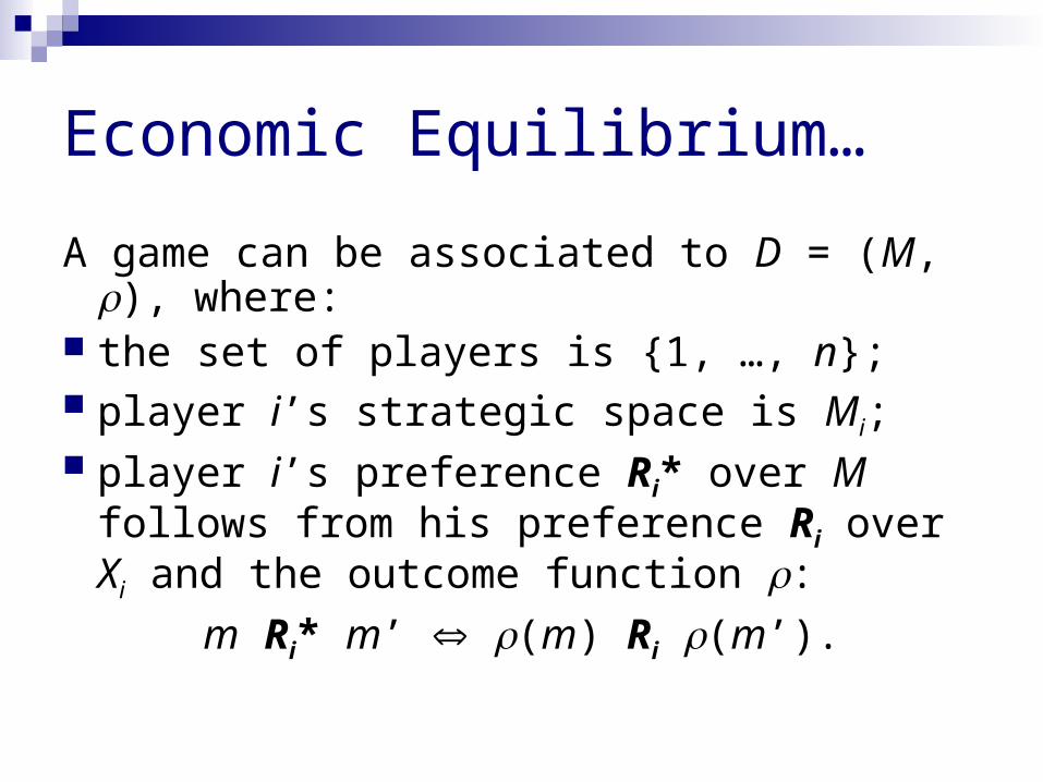
A game can be associated to D = (M, ), where: the set of players is {1, …, n}; player i’s strategic space is Mi; player i’s preference Ri* over M follows from

his preference Ri over Xi and the outcome function :

m Ri* m’ (m) Ri (m’).

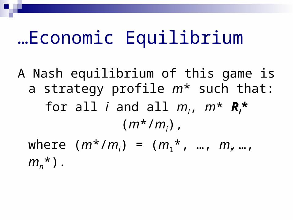
…Economic Equilibrium

A Nash equilibrium of this game is a strategy profile m* such that:

for all i and all mi, m* Ri* (m*/mi),

where (m*/mi) = (m1*, …, mi, …, mn*).

Lindahl Mechanism

Lindahl (1919) defines institutions, where the consumers are:

first given personal tax rates pi, chosen such that i pi = 1 to ensure budget balancing,

and then are asked to tell which amount yi of public goods they demand, knowing that they will pay pi per unit.

Lindahl Equilibrium

Lindahl (1919) forecasts that, endowed with such institutions, the behaviors of the consumers will drive the economy to a Lindahl equilibrium, defined as a list of personal tax rates (pi*)i, with i pi* = 1, and an allocation ((xi*)i, y*), such that, for all i:

(xi*, y*) Ri ((xi)i, y),for all (xi, y) Xi such that xi + pi* y ≤ wi.

The Free-Riding Problem

Samuelson (1966) rejects this forecast, by noting that Lindahl’s definition relies on the belief that each consumer truly thinks that he alone determines the supply of the public good and, thus, demands the amount that maximizes his preference, subject to his budget constraint.

This is unrealistic, for rational consumers should notice that they have an incentive to free-ride.

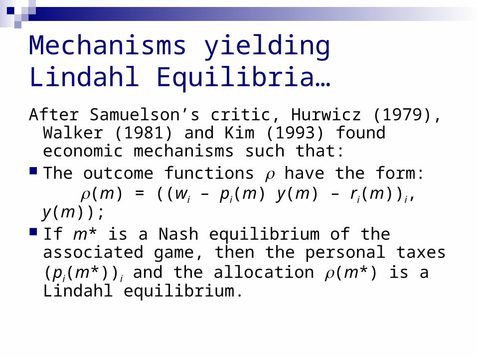
Mechanisms yielding Lindahl Equilibria…

After Samuelson’s critic, Hurwicz (1979), Walker (1981) and Kim (1993) found economic mechanisms such that:

The outcome functions have the form:(m) = ((wi – pi(m) y(m) – ri(m))i, y(m));

If m* is a Nash equilibrium of the associated game, then the personal taxes (pi(m*))i and the allocation (m*) is a Lindahl equilibrium.

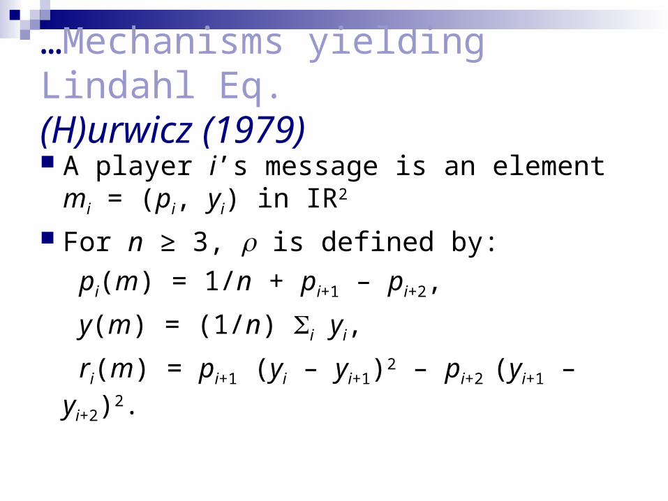
…Mechanisms yielding Lindahl Eq.(H)urwicz (1979)

A player i’s message is an element mi = (pi, yi) in IR2

For n ≥ 3, is defined by:

pi(m) = 1/n + pi+1 – pi+2,

y(m) = (1/n) i yi,

ri(m) = pi+1 (yi – yi+1)2 – pi+2 (yi+1 – yi+2)2.

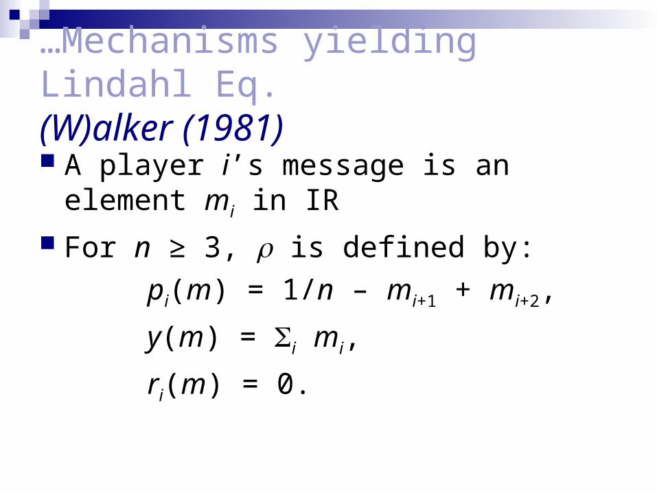
…Mechanisms yielding Lindahl Eq.(W)alker (1981)

A player i’s message is an element mi in IR

For n ≥ 3, is defined by:

pi(m) = 1/n – mi+1 + mi+2,

y(m) = i mi,

ri(m) = 0.

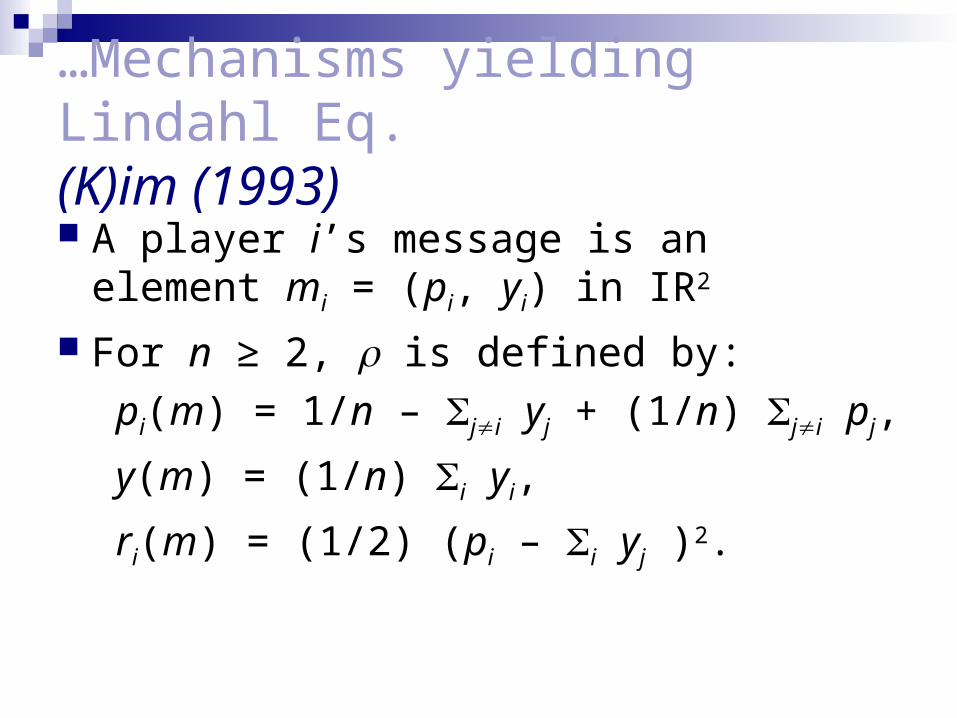
…Mechanisms yielding Lindahl Eq.(K)im (1993)

A player i’s message is an element mi = (pi, yi) in IR2

For n ≥ 2, is defined by:

pi(m) = 1/n – ji yj + (1/n) ji pj,

y(m) = (1/n) i yi,

ri(m) = (1/2) (pi – i yj )2.

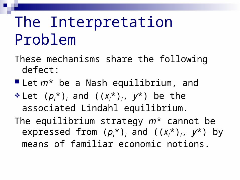
The Interpretation Problem

These mechanisms share the following defect: Let m* be a Nash equilibrium, and Let (pi*)i and ((xi*)i, y*) be the associated

Lindahl equilibrium.

The equilibrium strategy m* cannot be expressed from (pi*)i and ((xi*)i, y*) by means of familiar economic notions.

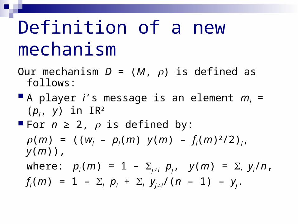
Definition of a new mechanism

Our mechanism D = (M, ) is defined as follows: A player i’s message is an element mi = (pi, y)

in IR2

For n ≥ 2, is defined by:

(m) = ((wi – pi(m) y(m) – fi(m)2/2)i, y(m)),

where: pi(m) = 1 – ji pj, y(m) = i yi/n,

fi(m) = 1 – i pi + i yji/(n – 1) – yj.

Using our mechanism…Avoiding the fines

The term (1/2) fi(m)2 plays the role of a fine.A player i’s goal is to escape it.Therefore, at a Nash equilibrium m*:

fi(m*) = 0, for all i.This implies that, at a Nash equilibrium m*:

pi* = pi(m*) and yi* = y(m*), for all i,

i pi* = 1.

Using our mechanism… Choosing the level of public good

Whatever m–i, a player i can find mi such that: he always pays pi(m) = 1 – ji pj per unit; he freely sets the supply y(m) = (1/n) i yi; he is not fined, i.e. (1/2) fi(m)2 = 0.Therefore, a Nash equilibrium m* will be such

that, for all i, y(m*) maximizes Ri, given pi(m*), and fi(m*) = 0.

Main results

Theorem 1. For an economy e, if the joint strategy m* = (pi*, yi*)i is a Nash equilibrium (of the game associated to D), then:

pi* = pi(m*) and yi* = y(m*), for all i;

the individualized prices (pi(m*))i and the allocation (m*) form a Lindahl equilibrium.

Main results

Theorem 2. For an economy e, if the individualized prices (pi*)i and the allocation ((xi*)i, y*) form a Lindahl equilibrium, then:

The joint strategy m* = (pi*, y*)i is a Nash equilibrium (of the game associated to D);

The mechanism D implements the Lindahl equilibrium, i.e. (m*) = ((xi*)i, y*).

Critic of the Nash equilibrium

The use of the Nash equilibrium concept to solve the game relies on the assumption that the players know both the rules of the game derived from D and the economy e.

This is most of the time unrealistic. In this case, Hurwicz (1972) argues that a Nash equilibrium could nevertheless result as an equilibrium point of a tâtonnement process.

Gradient process…

Let e be economy such that, for all i, the preferences Ri can be represented as a differentiable utility function Ui(xi, y).

If our mechanism D is used, for all m, the utility of i will be equal to:

ui(m) = Ui(wi – pi(m) y(m) – fi(m)2/2, y(m)).

…Gradient process

A gradient process describes the behavior of players who, in continuous time, adjust their strategy mi = (pi, yi), in the direction that maximizes the instantaneous increase of their utility ui(m), taking others’ strategies as given.

It is formalized as a dynamic system:

dmi/dt = dui(m)/dmi, mi(0) = mi0, for all i. (S)

Main results

Theorem 3. Let e be such that, for all i:

Ui(xi, y) = xi – vi(y), vi’(y) > 0 > vi’’(y).

If one exists, a Lindahl equilibrium of e, defined by (pi*)i and ((xi*)i, y*), is unique.

Then, m* = (pi*, y*)i is the unique stationary point of (S) and is globally stable.