Embed Size (px)
Citation preview

A COMPUTATIONAL ANALYSIS
OF OPTIMIZATION MODELS FOR
SUPPORT VECTOR MACHINES
LUCIA PETTERLE
RELATORE: Chiar.mo Prof. Matteo Fischetti
FACOLTA DI INGEGNERIA
CORSO DI LAUREA MAGISTRALE IN INGEGNERIA INFORMATICA
ANNO ACCADEMICO 2012/2013


A mia nonna Sergia.
Al mio papi e alla mia mami.


Abstract
The classification problem, known in the statistic field also as discriminant analysis
or recognition, is a theme of particular importance for problems resolution in the real
world. Possible examples are the medical diagnosis of the benign or malignant nature
of a disease, or the pattern image recognition.
As it is well known in the scientific literature for nearly two decades, a valid
approach to face the binary classification problem is the one represented by Support
Vector Machines. SVMs solve the learning problem by constructing a system which,
based on a subset of pre-categorized data and relative features, is able to classify
with high accuracy new, not already classified, data. From the mathematical point of
view, the SVM approach implies the resolution of a quadratic programming model.
The present thesis work consisted in a computational analysis, conducted via a
proper software implementation, of the mathematic behaviour of the aforesaid op-
timization model (equipped with the so-called Gaussian kernel); in a comparative
evaluation of the efficacy of approaches based on the resolution of alternative math-
ematical models (having in common the intent of reducing overfitting phenomenon);
and in a statistical evaluation of the accuracy superiority of a SVM approach classifi-
cation towards the use of a simpler but much less computationally expensive classifier.
The results we got revealed the intrinsic good nature of Gaussian kernel to be a
proper classifier by itself, a characteristic that limits the possible rooms for improve-
ment of accuracy results. We also found that SVM approach, with Gaussian kernel,
can boast just a 6% accuracy superiority over a simpler classification approach, that
does not require the computationally expensive resolution of a quadratic program-
ming optimization model. This observation, together with an analogous comparative
evaluation of the accuracy superiority of SVM approach using linear kernel, enabled
us to confirm the aforesaid thesis about Gaussian kernel nature. The previously col-
lected results allowed us to understand that the nature of the linear kernel could offer
more degrees of improvement and very preliminary tests seemed to confirm the va-
lidity of our alternative approaches. Eventually, the whole procedure produced lower
accuracies with respect to the SVM approach, so we leave this kind of approach as a
hint for further researches in this area.


Contents
Abstract 5
List of Figures 10
List of Tables 11
1 Introduction 15
1.1 Thesis scope . . . . . . . . . . . . . . . . . . . . . . . . . . . . . . . . . 15
1.2 Work focus . . . . . . . . . . . . . . . . . . . . . . . . . . . . . . . . . 15
1.3 Contents structure . . . . . . . . . . . . . . . . . . . . . . . . . . . . . 16
2 A short introduction to the Classification Problem 17
2.1 Areas of interest . . . . . . . . . . . . . . . . . . . . . . . . . . . . . . 17
2.2 Description of the problem . . . . . . . . . . . . . . . . . . . . . . . . . 17
2.2.1 Discriminations in theme of classification . . . . . . . . . . . . 19
2.3 Classifier . . . . . . . . . . . . . . . . . . . . . . . . . . . . . . . . . . . 20
2.3.1 Steps of the classification problem . . . . . . . . . . . . . . . . 20
2.3.2 K-fold cross validation . . . . . . . . . . . . . . . . . . . . . . . 21
2.3.3 Leave-one-out . . . . . . . . . . . . . . . . . . . . . . . . . . . . 21
2.4 Mathematical formalization of the problem . . . . . . . . . . . . . . . 22
2.4.1 Learning procedure . . . . . . . . . . . . . . . . . . . . . . . . . 22
2.5 Parameters for the evaluation of a classifier . . . . . . . . . . . . . . . 23
2.5.1 Goodness and comparison measurements for binary classifiers . 24
2.5.1.1 Notation . . . . . . . . . . . . . . . . . . . . . . . . . 24
2.5.1.2 Different possible error measurements . . . . . . . . . 24
3 What a SVM is and
how it solves the classification problem 29
3.1 Some history . . . . . . . . . . . . . . . . . . . . . . . . . . . . . . . . 29
3.2 A short description . . . . . . . . . . . . . . . . . . . . . . . . . . . . . 29
3.3 How a SVM solves the classification problem . . . . . . . . . . . . . . 30
3.3.1 Classifier on linearly separable data . . . . . . . . . . . . . . . 31

8 CONTENTS
3.3.2 Classifier on non linearly separable data . . . . . . . . . . . . . 37
3.3.2.1 Linear classifier on non linearly separable data . . . . 38
3.3.2.2 Non linear classifier on non linearly separable data . . 40
4 Alternative training models 47
4.1 Gaussian kernel models . . . . . . . . . . . . . . . . . . . . . . . . . . 47
4.1.1 SVM aINT . . . . . . . . . . . . . . . . . . . . . . . . . . . . . 48
4.1.2 SVM TV . . . . . . . . . . . . . . . . . . . . . . . . . . . . . . 49
4.1.3 SVM TV aINT . . . . . . . . . . . . . . . . . . . . . . . . . . . 49
4.1.4 SVM aAll TV . . . . . . . . . . . . . . . . . . . . . . . . . . . . 50
4.1.5 SVM Mixed . . . . . . . . . . . . . . . . . . . . . . . . . . . . . 50
4.1.6 SVM MixedMu . . . . . . . . . . . . . . . . . . . . . . . . . . . 51
4.2 Linear kernel models . . . . . . . . . . . . . . . . . . . . . . . . . . . . 52
4.2.1 SVM K-lin . . . . . . . . . . . . . . . . . . . . . . . . . . . . . 52
4.2.2 SVM K-lin wINT . . . . . . . . . . . . . . . . . . . . . . . . . . 52
5 Experimental tests and results 55
5.1 Real world datasets . . . . . . . . . . . . . . . . . . . . . . . . . . . . . 55
5.1.1 Preprocessing on raw data . . . . . . . . . . . . . . . . . . . . . 55
5.1.2 Experimental choices for data training . . . . . . . . . . . . . . 58
5.1.3 Availability of the data on the web . . . . . . . . . . . . . . . . 58
5.2 Comparison between
SVM approach and A1B0 approach . . . . . . . . . . . . . . . . . . . . 59
5.2.1 A1B0 approach
59
5.2.2 Parameters setting: γ = 0.1 . . . . . . . . . . . . . . . . . . . . 59
5.2.3 Organization of the tests . . . . . . . . . . . . . . . . . . . . . . 60
5.3 Experimental results for tests described in section 5.2 . . . . . . . . . 61
5.3.1 Statistical significance of the difference between
the two methods . . . . . . . . . . . . . . . . . . . . . . . . . . 61
5.3.2 Some statistical considerations about the comparison of
the two methods . . . . . . . . . . . . . . . . . . . . . . . . . . 62
5.3.2.1 Datasets level . . . . . . . . . . . . . . . . . . . . . . 62
5.3.2.2 Higher global level . . . . . . . . . . . . . . . . . . . . 63
5.4 Experimental results for tests described in chapter 4 . . . . . . . . . . 65
5.4.1 Results with Gaussian kernel . . . . . . . . . . . . . . . . . . . 66
5.4.2 Results with linear kernel . . . . . . . . . . . . . . . . . . . . . 73
5.5 Final comments over the results . . . . . . . . . . . . . . . . . . . . . . 73

CONTENTS 9
6 Software 75
6.1 Used software . . . . . . . . . . . . . . . . . . . . . . . . . . . . . . . . 75
6.1.1 CPLEX . . . . . . . . . . . . . . . . . . . . . . . . . . . . . . . 75
6.1.1.1 Command line code . . . . . . . . . . . . . . . . . . . 76
6.1.1.2 lp file format . . . . . . . . . . . . . . . . . . . . . . . 77
6.1.1.3 .sol file format . . . . . . . . . . . . . . . . . . . . . . 78
6.1.2 SVMlight . . . . . . . . . . . . . . . . . . . . . . . . . . . . . . . 80
6.1.2.1 SVMlight installation and use . . . . . . . . . . . . . . 80
6.1.2.2 SVMlight file format . . . . . . . . . . . . . . . . . . . 82
6.1.3 LIBSVM . . . . . . . . . . . . . . . . . . . . . . . . . . . . . . 83
6.1.3.1 LIBSVM installation and use . . . . . . . . . . . . . . 83
6.1.3.2 LIBSVM file format . . . . . . . . . . . . . . . . . . . 85
6.1.4 R . . . . . . . . . . . . . . . . . . . . . . . . . . . . . . . . . . . 86
6.1.4.1 Command line code . . . . . . . . . . . . . . . . . . . 86
6.2 Implemented software . . . . . . . . . . . . . . . . . . . . . . . . . . . 88
6.2.1 C source code . . . . . . . . . . . . . . . . . . . . . . . . . . . . 88
6.2.2 Scripts . . . . . . . . . . . . . . . . . . . . . . . . . . . . . . . . 94
6.2.3 Hardware specifications . . . . . . . . . . . . . . . . . . . . . . 94
6.3 Instructions for compilation and execution of C source code . . . . . . 95
6.3.1 Directories structure . . . . . . . . . . . . . . . . . . . . . . . . 95
6.3.2 Where to save files . . . . . . . . . . . . . . . . . . . . . . . . . 96
6.3.3 How to make the code work . . . . . . . . . . . . . . . . . . . . 97
6.3.3.1 Prerequisites . . . . . . . . . . . . . . . . . . . . . . . 97
6.3.3.2 Instructions for scripts runs . . . . . . . . . . . . . . . 98
Conclusions and future perspectives 99
A Detailed results for tests described in section 5.2 101
B A statistical tool: Wilcoxon Test 113
B.1 Prerequisites and hypothesis . . . . . . . . . . . . . . . . . . . . . . . . 113
B.2 Procedure . . . . . . . . . . . . . . . . . . . . . . . . . . . . . . . . . . 114
B.3 An example to describe the mathematical steps of the test . . . . . . . 115
C More detailed results 119
D Scripts 127
D.1 Example 1 . . . . . . . . . . . . . . . . . . . . . . . . . . . . . . . . . . 127
D.2 Example 2 . . . . . . . . . . . . . . . . . . . . . . . . . . . . . . . . . . 130

10 CONTENTS
E C Code 133
E.1 Example of Model constructor . . . . . . . . . . . . . . . . . . . . . . 133
F Table of the normal distribution 139
Bibliography 139
Acknowledgements 145
List of Figures
2.1 Multiclass cancer classification scheme. . . . . . . . . . . . . . . . . . . 18
2.2 Learning procedure scheme. . . . . . . . . . . . . . . . . . . . . . . . . 23
2.3 Underfitting and overfitting. . . . . . . . . . . . . . . . . . . . . . . . . 26
2.4 a. It is always possible to linearly separate three points. b. It is not
always possible for four points. So the VC dimension in this case is 3. 26
2.5 Tradeoff of the structural risk minimization. . . . . . . . . . . . . . . . 26
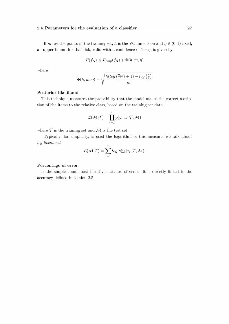
3.1 A generical separating hyperplane. . . . . . . . . . . . . . . . . . . . . 31
3.2 The optimum separating hyperplane. . . . . . . . . . . . . . . . . . . . 32
3.3 Distance point x - hyperplane g(x) = 0. . . . . . . . . . . . . . . . . . 32
3.4 Non linearly separable dataset. . . . . . . . . . . . . . . . . . . . . . . 37
3.5 Non linearly separable dataset with a linear separation. . . . . . . . . 38
3.6 The SVM trick for non linearly separable data. . . . . . . . . . . . . . 41
3.7 Gaussian kernel value vs distance, for the parameter γ = 0.1, 1, 10, 100. 44
3.8 Signals analogy. . . . . . . . . . . . . . . . . . . . . . . . . . . . . . . . 45
6.1 Example of CPLEX LP file. . . . . . . . . . . . . . . . . . . . . . . . . 77
6.2 Example of CPLEX output file. . . . . . . . . . . . . . . . . . . . . . . 78
6.3 Example of use of CPLEX interactive optimizer. . . . . . . . . . . . . 79
6.4 Example of use of the modules svm learn and svm classify of SVMlight . 81
6.5 Pattern line of SVMlight input files. . . . . . . . . . . . . . . . . . . . . 82
6.6 Example line of SVMlight input files. . . . . . . . . . . . . . . . . . . . 82
6.7 Example of use of the LIBSVM Python script. . . . . . . . . . . . . . 84
6.8 Example of a graphical classification representation obtained with LIB-
SVM. . . . . . . . . . . . . . . . . . . . . . . . . . . . . . . . . . . . . 84
6.9 Example of LIBSVM input file. . . . . . . . . . . . . . . . . . . . . . . 87
6.10 Significative output lines from R software for Wilcoxon test. . . . . . . 87
6.11 Scheme flow for our SVM implementation. . . . . . . . . . . . . . . . . 89

12 LIST OF FIGURES

List of Tables
5.1 Datasets: names, number of instances, number of attributes. . . . . . . 56
5.2 p-values for comparison between SVM approach and A1B0 approach. . 61
5.3 Results for each dataset for comparison SVM vs A1B0. . . . . . . . . . 62
5.4 Global results for comparison SVM vs A1B0. . . . . . . . . . . . . . . 64
5.5 Accuracy with SVM approach. . . . . . . . . . . . . . . . . . . . . . . 65
5.6 Global results for comparison SVM vs A1B0 with linear kernel. . . . . 67
5.7 Accuracy with SVM aINT approach. . . . . . . . . . . . . . . . . . . . 68
5.8 Accuracy with SVM TV aINT approach. . . . . . . . . . . . . . . . . . 69
5.9 Accuracy with SVM TV approach. . . . . . . . . . . . . . . . . . . . . 70
5.10 Accuracy with SVM Mixed approach. . . . . . . . . . . . . . . . . . . . 70
5.11 Accuracy with SVM aAll TV approach. . . . . . . . . . . . . . . . . . 71
5.12 Accuracy with SVM MixedMu approach. . . . . . . . . . . . . . . . . . 71
5.13 All obtained accuracies, with Gaussian kernel. . . . . . . . . . . . . . . 72
5.14 Accuracy with SVM K-lin approach. . . . . . . . . . . . . . . . . . . . 73
5.15 Accuracy with SVM K-lin wINT approach. . . . . . . . . . . . . . . . 74
A.1 Comparison table for dataset Adult. . . . . . . . . . . . . . . . . . . . 102
A.2 Comparison table for dataset Australian. . . . . . . . . . . . . . . . . . 103
A.3 Comparison table for dataset Breast Mangasarian and Wolberg. . . . . 104
A.4 Comparison table for dataset Bupa. . . . . . . . . . . . . . . . . . . . 105
A.5 Comparison table for dataset German. . . . . . . . . . . . . . . . . . . 106
A.6 Comparison table for dataset Heart. . . . . . . . . . . . . . . . . . . . 107
A.7 Comparison table for dataset Ionosphere. . . . . . . . . . . . . . . . . 108
A.8 Comparison table for dataset Pima. . . . . . . . . . . . . . . . . . . . 109
A.9 Comparison table for dataset Sonar. . . . . . . . . . . . . . . . . . . . 110
A.10 Comparison table for dataset Wdbc Mangasarian and Wolberg. . . . . 111
A.11 Comparison table for dataset Wpbc Mangasarian and Wolberg. . . . . 112
B.1 Wilcoxon test table for a small sample on Wpbc Mangasarian and
Wolberg dataset. . . . . . . . . . . . . . . . . . . . . . . . . . . . . . . 116

14 LIST OF TABLES
C.1 Accuracies for SVM approach, Gaussian kernel. . . . . . . . . . . . . . 121
C.2 Accuracies for SVM approach, linear kernel. . . . . . . . . . . . . . . . 123
C.3 Detailed accuracies for MIP alternative approach with linear kernel. . 125

Chapter 1
Introduction
1.1 Thesis scope
The context of the present work belongs to that discipline of the Artificial Intelligence
known in the scientific literature as machine learning. And, specifically, it concerns the
so-called classification problem. The classification problem, starting from a historical
set of observations (or points or items), each constituted by a set of elements values,
named features (or attributes), and a relative category, named class, consists in the
assignment of new experimental items to the class considered to be the most correct.
The theme of classification has lots of variants and the one we are interested in is
classification with just two possible classes for each observation: binary classification.
We will concentrate on the approach proposed by Vladimir Vapnik and his colleagues
in the 90s, called Support Vector Machines approach.
1.2 Work focus
Our work focuses on the mathematical background that constitutes the algorithmic
bases of the functionality of Support Vector Machines. Their operational procedure,
that will be described in detail in Chapter 3, refers to the resolution of a quadratic
programming problem, whose formulation is strictly related to the choice of the so-
called kernel function. It is the key idea on which is based the use of Support Vector
Machines as linear classifiers: as a matter of fact, it permits to transform the original
features space, where classification can become very arduous, in an equivalent space,
where classification can be realized through a simple linear classifier.
First of all in our analysis, that required the implementation of the necessary
software and the utilization of appropriated tools for mathematical optimization and
statistical evaluations, we investigated in details the behaviour and the role of the
Gaussian kernel in the classification procedure.
Secondly, analyzing the values assumed by the classification parameters after the

16 Introduction
resolution of the aforesaid quadratic programming problem, we made the hypothesis
that this approach could have the collateral effect of taking the system to an overfitting
behaviour. Therefore, in the aim of reducing the impact of this phenomenon, we
planned, implemented and tested alternative mathematical models.
Afterward we shifted our focus to the analysis of the behaviour of the linear kernel.
We compared the performance of the system equipped with the classical quadratic
model, using linear kernel, with an alternative approach, based on the resolution of a
mixed-integer programming problem, aimed again at the reduction of the overfitting
problem.
Eventually, we treated an evaluation of the superiority, in terms of accuracy, of
the approach adopted by Support Vector Machines that, as previously said, implies
the resolution of a quadratic programming problem, towards a much more simplified
approach, based on the offline setting of the classification parameters, which can be
implemented with an exiguous number of code lines and that requires a very small
computational effort.
1.3 Contents structure
In the following we introduce briefly the global structure and the chapter contents of
this thesis.
In Chapter 2 we face a panoramic introduction, from the theoretical point of view,
of the theme of machine learning and the problem of classification, pointing out the
specific aspects on which our focus will be based.
In Chapter 3 we get a deeper sight in a detailed description, from the mathematical
point of view, of the approach adopted by Support Vector Machines.
In Chapter 4 we present the alternative approaches we propose to the original
SVM approach. We describe the mathematical models tested, motivating the aim of
their formulation.
In Chapter 5 we describe the practical effort and the experimental work performed
in this thesis, motivating the choices also on theoretical basis, and we provide and
analyse the collected experimental results.
In Chapter 6 we treat the characteristics and the modality of use of the software
we implemented to perform the experimental tests, in addition to the software that
was necessary to implement to interface properly to the first one, and to guarantee
an adequate automatization of tests procedures.
In the Appendices we report the experimental results at a larger level of detail,
an exemplificative C source code listing and some scripts that were necessary to
implement in order to automatize the whole experimental procedures.

Chapter 2
A short introduction to theClassification Problem
2.1 Areas of interest
First of all let us identify the proper areas related to the classification problem.
There are several contexts in applications where it is very important to construct
a system which is able to learn how to classify correctly a set of items, using the most
significative parameters that characterize the items themselves.
Examples of those contexts are:
The medical field: a system that, based on a sufficient set of past clinical data,
is able to discover if a patient is affected by a specific disease (those kinds of
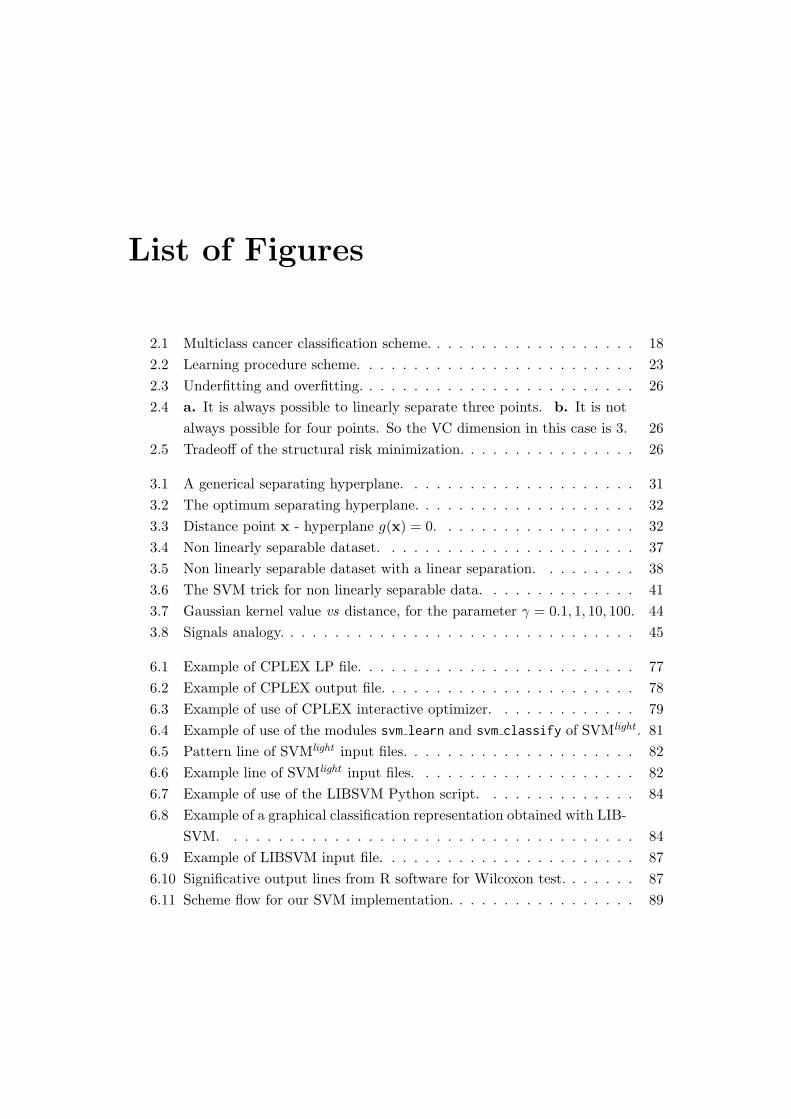
systems are really useful in the diagnosis of cancer – see figure 2.1);
The Information Retrieval field: a system that is able to decide if a text is rele-
vant for a specific topic, based on the terms that appear in it;
The image classification field: a system that, based on a small set of points of a
simple drawn, is able to reconstruct the pattern below it;
The economical field: a system that is able to determinate different typologies of
clients (to produce targeted advertising campaigns).
2.2 Description of the problem
Classification problem is
A process for grouping a set of data into groups so that data within a
group have high similarity and, at the same time, quite high dissimilarity
from data in other groups [2].
18 A short introduction to the Classification Problem
Figure 2.1: Multiclass cancer classification scheme.

2.2 Description of the problem 19
Classification technique is the most commonly used technique to analyze large sets
of data in automatic or semi-automatic way, with the purpose of extracting knowledge
from them.
The ascription of a single item to a specific class is the result of a procedure known
as learning procedure. Typically, a learning procedure is realized by a learning ma-
chine that, observing an already classified training set of data, constructs an operator
that is able to predict the output y for each input x not belonging to the aforesaid
training set.
2.2.1 Discriminations in theme of classification
We can make several distinctions in theme of classification.
Multi class vs binary classification
There are different problems of classification:
� With several possible classes the single item can belong to: multi class classifi-
cation;
� With only two possible classes the single item can belong to: binary classifica-
tion.
For simplicity we consider only problems of the second type, because they are the
problems of interest for our SVM-oriented theoretical overview.
Supervised vs unsupervised classification
This is perhaps the most important distinction in classification problems:
� In supervised classification we know the possible groups and we have data al-
ready classified, being used overall for training. The problem consists in associ-
ating the data in the most appropriate group taking advantage of those already
labeled.
� In unsupervised classification, also-called clustering, possible groups (or clusters)
are not known in advance, and the data available are not classified. The goal
is then to classify in the same cluster the data considered as similar.
We will consider only supervised classification, that is the one used by the SVM
approach.
Generative vs discriminative classification methods
We can distinguish two different approaches:

20 A short introduction to the Classification Problem
� Discriminative methods: building a boundary between the classes, they di-
rectly model the posterior probability P (Z|X); the empirical observations are
explained by the model that describes probabilistically the interaction between
the variables of the problem;
� Generative methods: deducing the a posteriori probability through the Bayes’
Rule, they first model the joint probability distribution P(X,Z); they deal di-
rectly with the problem of finding the criteria that permit to group together
the empirical observations.
The first approach is the one used by Support Vector Machines.
2.3 Classifier
We refer to the algorithm that realizes classification as classification function or clas-
sifier.
The purpose, in the determination of the classifier, is to minimize the classification
error : it occurs when an item x is assigned to a class Ci, but actually it belongs to
another class Cj . We will talk about different kinds of errors to be minimized in
2.5.1.2.
2.3.1 Steps of the classification problem
In the solution of classification problem we can recognize three fundamental phases:
� construction of a model that describes a certain set of classes after the analysis
of some of the multi-dimensional items, through their features: this phase is
also-called learning phase ;
� evaluation of the constructed model on other items;
� use of the aforesaid model to classify new items: this phase is also-called clas-
sification phase .
Given a dataset of points and relative classification, two particular subsets, always
strictly disjoint, are taken from the original dataset to implement the learning proce-
dure:
Training set: it permits to train the system, so that it is possible to find the most
appropriate classification function (it is used during the learning phase);
Test set: it permits to realize an estimation of the accuracy of the classification
function previously defined (it is used during the classification phase).
Some classification methods further divide the training set in k disjoined subsets to
perform the so-called k-fold cross validation.
2.3 Classifier 21
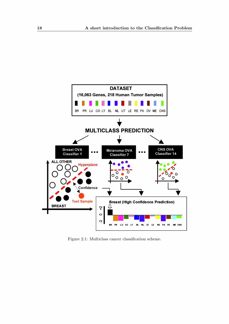
2.3.2 K-fold cross validation
Classification techniques often involve the use of special parameters, that can either
be defined “offline” or chosen, through a trial-and-error procedure, by the algorithm.
Choosing the second possibility, they can be determined before the final training
procedure, during the so-called validation phase , in the most proper way in order
to give the best classification results.
One of the possible ways to choose the optimal parameters setting is to perform
the so-called k-fold cross validation.
Cross-validation is a computer intensive technique, introduced in [4]. It mimics
the use of training and test sets by repeatedly training the algorithm k times with a
fraction 1k of training examples left out for testing purposes.
Analytically, it consists in:
� extracting n·(k−1)k items from the training set (where n is its dimension);
� constructing a classification rule over the extracted items;
� classifying the remaining nk items obtaining the related accuracy;
� re-start again from point 1 the whole procedure, k times.
In our experimentation we used 5-fold cross validation that consists in randomly
dividing the training set into 5 disjoined subsets: in turn, 4 of the 5 aforesaid subsets
assume the role of training set and the remaining subset the role of the so-called
validation set.
Training method is now applied to the previously described training set, and the
classification phase takes place over the validation set. This procedure is repeated 5
times, in turn changing the training-validation role by the different fractions of the
original training set.
After the completion of the 5 phases, the mean value of the accuracies obtained for
each parameter setting is computed: the best mean accuracy obtained identifies the
optimal parameter setting to be used during the subsequent learning and classification
phases. After validation, the learning procedure is applied over the whole training
plus validation set, while classification will take place over the test set.
As terminology can be confusing, let us recap the concepts just explained: vali-
dation technique involves to select randomly a fraction of 45 of the training set and to
call again this portion “training set” during the validation phase, while “validation
set” refers to the complementary portion acting as a fictitious test set.
2.3.3 Leave-one-out
This is a validation technique alternative to the previously described K-fold cross
validation [6].
22 A short introduction to the Classification Problem
The only difference between the two approaches is that leave-one-out extracts just
a single item to be excluded from the training set use during the validation phase.
That is, the validation set in each iteration is composed by a single element.
Leave-one-out is more computationally expensive than K-fold cross validation
because the aforesaid procedure has to be repeated n times (where n is the dimension
of the training set), since each single item of the training set has to be classified
during the validation.
Scientific experimentations affirm that the efficacy of leave-one-out can be com-
pared to that of K-fold cross validation [25].
2.4 Mathematical formalization of the problem
Considering just binary classification (classification problem in presence of only two
possible alternatives), we can formalize the problem as in the following:
Formalization of the classification problem
Let X be a generic set (usually X = Rn).
Let T = {(xi, yi), i = 1, . . . ,m} ⊂ X × {+1,−1} be a set of couples that
we call training set.
We want to determinate a map δ : X −→ {+1,−1}, that implements the
right association between an item x that does not belong to the training
set and the class y it is associated to with highest probability.
So, classification aims at building a decision rule δ:
δ : X −→ {+1,−1}
x 7→ y = δ(x)
2.4.1 Learning procedure
Given a set of pre-classified examples (the training set):
(x1, y1), . . . , (xm, ym)
where xi ∈ Rn and yi ∈ {−1,+1}, a learning machine realizes a class of functions fΛ,
each of that is identified by a set of parameters (the vector Λ).
The learning procedure consists in choosing, between those functions, the one that
is the most appropriate. Obviously the choice of a function is equivalent to the choice
of a set of optimal parameters Λ.
Formally, a learning machine is given by the set of functions:
fΛ : R −→ {−1, 1}
This procedure has the purpose of choosing the fΛ∗ that realizes “the best clas-
sification”.

2.5 Parameters for the evaluation of a classifier 23
Figure 2.2: Learning procedure scheme.
2.5 Parameters for the evaluation of a classifier
Below we itemize some parameters that enable us to evaluate a particular classifier.
� ACCURACY:
Accuracy =truepositiveclass1 + truepositiveclass−1
|class1|+ |class− 1|It represents the percentage of instances correctly classified, whose predicted
class coincides with the real one.
� PRECISION:
Precisionclass1 =truepositiveclass1
truepositiveclass1 + falsepositiveclass1
It is a measure of correctness.
The lower the number of false positives, the higher (the closer to 1) the precision.
� RECALL:
Recallclass1 =truepositiveclass1
truepositiveclass1 + falsenegativeclass1
It is a measure of completeness.
The lower the number of false negatives, the higher (the closer to 1) the recall.
� F-MEASURE:
F −Measureclass1 =2 ·Recallclass1 · Precisionclass1
Recallclass1 + Precisionclass1

24 A short introduction to the Classification Problem
2.5.1 Goodness and comparison measurements for binary classifiers
Up to now we have talked about “the most appropriated class” an item can be assigned
to. It is important to understand on which bases a binary classifier is intended to be
a “good” classifier: to choose between the possible fΛ we mentioned in 2.4.1, we have
to define a quality criterion.
As we can imagine intuitively, the goodness of a classifier is inversely proportional
to the errors it commits (quantitatively and qualitatively).
2.5.1.1 Notation
We will use to talk about classification in an intuitive way: we will consider classifica-
tion as a data mining problem that aims to determinate the membership of different
points to different sets.
We have a set of points (about some hundreds of points) expressed as vectors of
n coordinates in the n-dimensional space.
We have to realize a binary classification for those points. So we have to assign
to each point a value in {+1,−1}, to indicate the membership of the relative item to
a specific set, which we call also class.
2.5.1.2 Different possible error measurements
There are several possibilities in measuring that kinds of errors. We itemize the
possible error measurements and describe more deeply some of them:
� Empirical error minimization;
� Structural risk minimization;
� Posterior likelihood;
� Percentage of error.
Empirical error minimization.
First of all let us define:
Loss function: L(y, fΛ(x)) = L(y,Λ,x)
it measures the gap between the predicted value fΛ(x) and the real one
y.
Examples of loss function for fΛ(x) : Rn −→ {−1, 1} are:
� Misclassification error, first type:
L(y, fΛ(x)) ={
0 fΛ(x) = y1 fΛ(x) = y
2.5 Parameters for the evaluation of a classifier 25
� Misclassification error, second type:
L(y, fΛ(x)) =1
2|fΛ(x)− y|
� Logistic loss:
L(y, fΛ(x)) = ln(1 + e−(y·f(x))
)What we want to minimize is the effective risk or theoretical error, committed on
the different choices of the vector Λ; it can be viewed also as the expected value of
the loss we have choosing a particular function.
R(Λ) = R(fΛ) = E [L(y, fΛ(x)] =∫
L(y, fΛ(x)P (x, y)dxdy
Since the join probability distribution P (x, y) is not known, we are not able to cal-
culate the theoretical error. However we know a set of m empirical observations
(independent and identically distributed – the data of the training set) that permit
us to calculate the empirical error or empirical risk.
Remp(fΛ) =1
m
m∑i=1
L(yi, fΛ(xi))
For the Big Numbers Law we know that
limm→∞
Remp(fΛ) = R(fΛ)
So we can minimize the empirical error instead of the theoretical one.
The function that minimizes the empirical error is not unique. We can decide to
choose functions of different complexities, but the complexity degree is related to two
particular phenomenons:
� Overfitting : when the class of functions fΛ(x) is too complex we will not have
a good approximation of the function on the test set;
� Underfitting : when the class of functions fΛ(x) is too simple we will not have
a good approximation of the function on the training set.
Structural risk minimization.
First of all let us introduce the notion of VC dimension (whose name refers to the
scientists Vapnik and Chervonenkis) [17].
VC dimension (of a binary classifier): is the maximum number of items
of the training that the classifier (with a proper function fΛ(x)) is able
to separate into two classes; informally it can be intended as a sort of
complexity of the classifier.

26 A short introduction to the Classification Problem
Figure 2.3: Underfitting and overfitting.
Figure 2.4: a. It is always possible to linearly separate three points. b. It is notalways possible for four points. So the VC dimension in this case is 3.
Below, in figure 2.4, we can see that the VC dimension of a linear classifier in R2 is
3: in fact we can always separate 3 points with a rect, but no more than 3.
The SVM approach [15] [16] tries to minimize at the same time the empirical error
and the complexity of the classifier: this tradeoff approach is called minimization of
the structural risk, as we can see in figure 2.5.
Figure 2.5: Tradeoff of the structural risk minimization.
2.5 Parameters for the evaluation of a classifier 27
If m are the points in the training set, h is the VC dimension and η ∈ (0, 1) fixed,
an upper bound for that risk, valid with a confidence of 1− η, is given by
R(fΛ) ≤ Remp(fΛ) + Φ(h,m, η)
where
Φ(h,m, η) =
√h(log
(2mh
)+ 1)− log
(η4
)m
Posterior likelihood
This technique measures the probability that the model makes the correct ascrip-
tion of the items to the relative class, based on the training set data.
L(M|T ) =
m∏i=1
p(yi|xi, T ,M)
where T is the training set and M is the test set.
Typically, for simplicity, is used the logarithm of this measure, we talk about
log-likelihood
L(M|T ) =m∑i=1
log[p(yi|xi, T ,M)]
Percentage of error
Is the simplest and most intuitive measure of error. It is directly linked to the
accuracy defined in section 2.5.

28 A short introduction to the Classification Problem

Chapter 3
What a SVM is andhow it solves the classificationproblem
3.1 Some history
Support Vector Machines were introduced by Vladimir Vapnik and colleagues (Boser
and Guyon) in the late 70s.
The earliest mention was in [Vapnik, 1979], but the first main paper seems to be
[Vapnik, 1995].
The theoretical bases were developed from Statistical Learning Theory (Vapnik
and Chervonenkis) since the 60s.
Empirically they immediately showed good performances: successful applications
in many fields (bioinformatics, text, image recognition, . . . ).
3.2 A short description
A Support Vector Machine is defined as
A binary classifier that is able to learn the bound between elements that
belong to two different classes [19].
The SVM approach can be thought as an alternative learning technique to poly-
nomial, radial basis function and multi-layer perceptron classifiers.
SVMs are sets of supervised learning methods whose training technique permits
to represent complex non linear functions. The characteristic parameters of the sys-
tem are determined solving a quadratic convex optimization problem. That SVM
has the “mathematical advantage” of having a global minimum: it ensures that the
resulting parameters are actually the best that can be found for the problem, given
the particular training set.

30What a SVM is and
how it solves the classification problem
The purpose of SVM is to perform a classification by constructing a n-dimensional
hyperplane that optimally separates the data (the points) into two categories.
With reference to the description we will do in 3.3.2.2 about non linear classifiers
on non linearly separable data, SVM were originally defined for the classification in
classes of objects that are linearly separable, but obviously they can be used also to
separate classes of elements non linearly separable, making them really interesting in
the scientific environment.
Summarizing, the functionality of a SVM depends on three factors:
The kernel type specific for a particular problem: it enables the system to classify
properly also non linearly separable data;
The optimization model that works on the training set, but provides robust val-
ues Λ and b parameters, that can be adequate also to the classification of the
test set items;
The setting of parameters γ and C that is realized by a trial-and-error valida-
tion procedure and represents the most difficult part in the use of SVM.
For a mathematical description of SVM approach see section 3.3 [7] [8] [9] [10] [11].
3.3 How a SVM solves the classification problem
Given the training set
T = {(xi, yi) | xi ∈ Rn, yi ∈ {−1,+1}, i = 1, . . . ,m}
and a properly tuned parameter C, the SVM approach solves the following optimiza-
tion problem
minξ,b,w Cm∑i=1
ξi +1
2||w||2
yi(wTxi + b) ≥ 1− ξi i = 1, . . . ,m
ξi ≥ 0 i = 1, . . . ,m
b ∈ R
w ∈ Rn
We will deal with the dual of the problem above, which is
maxλ
l∑i=1
λi −1
2
l∑i,j=1
λiλjyiyjxixj
l∑i=1
λiyi = 0
0 ≤ λi ≤ C i = 1, . . . , l
3.3 How a SVM solves the classification problem 31
To understand the theory the model above is based on, we have to clarify how to
deal with linearly and non linearly separable data.
3.3.1 Classifier on linearly separable data
We want to find the hyperplane H, identified by the parameters (w, b), that separates
the data in the best way: it has to be as far as possible by each point xi to be
separated.
For the training set represented in figures below, figure 3.1 shows one of the infinite
hyperplanes that separate the linearly separable points of the dataset, and figure 3.2
shows the optimum one among them.
Figure 3.1: A generical separating hyperplane.
The distance between a point x and hyperplane (w, b) is:
d(x, (w, b)) =|wT · x+ b|
||w||
Explanation of the result.
Let us explain the result got above, helping with figure 3.3.
We have:
� A hyperplane H, defined by a linear discriminant function:
g(x) = wTx+ b = 0

32What a SVM is and
how it solves the classification problem
Figure 3.2: The optimum separating hyperplane.
Figure 3.3: Distance point x - hyperplane g(x) = 0.
� A point x, defined by a n-dimensional vector, whose distance from
H we want to calculate.

3.3 How a SVM solves the classification problem 33
Using the vectorial sum we can express x as
x = xp + xn
where xp is the component parallel to the hyperplane and xn is the
normal one;
� A unitary norm vector, normal to the hyperplane H
w′ =w
||w||.
The parallel component xp is the orthogonal projection of x on the hy-
perplane H.
We can express the component that is normal to the hyperplane as
xn = r ·w′ = r · w
||w||
Where r is the algebraic distance between x and H.
So we can write
x = xp + r · w
||w||
Using that decomposition of x we find that
g(x) = wTx+ b = wT · (xp + r · w
||w||) + b =
= wTxp + b+ r · wTw
||w||=
= g(xp) + r · wTw
||w||Since the vector g(xp) lies on the hyperplane (and so we have that g(xp) =
0) and since the inner product wTw is equal to ||w||2, we can simplify
the expression above finding that
g(x) = r · ||w||
And so that
r =g(x)
||w||=
wTx+ b
||w||Since a distance is always expressed as a positive value
r =|wTx+ b|
||w||
That is what we wanted to explain.
34What a SVM is and
how it solves the classification problem
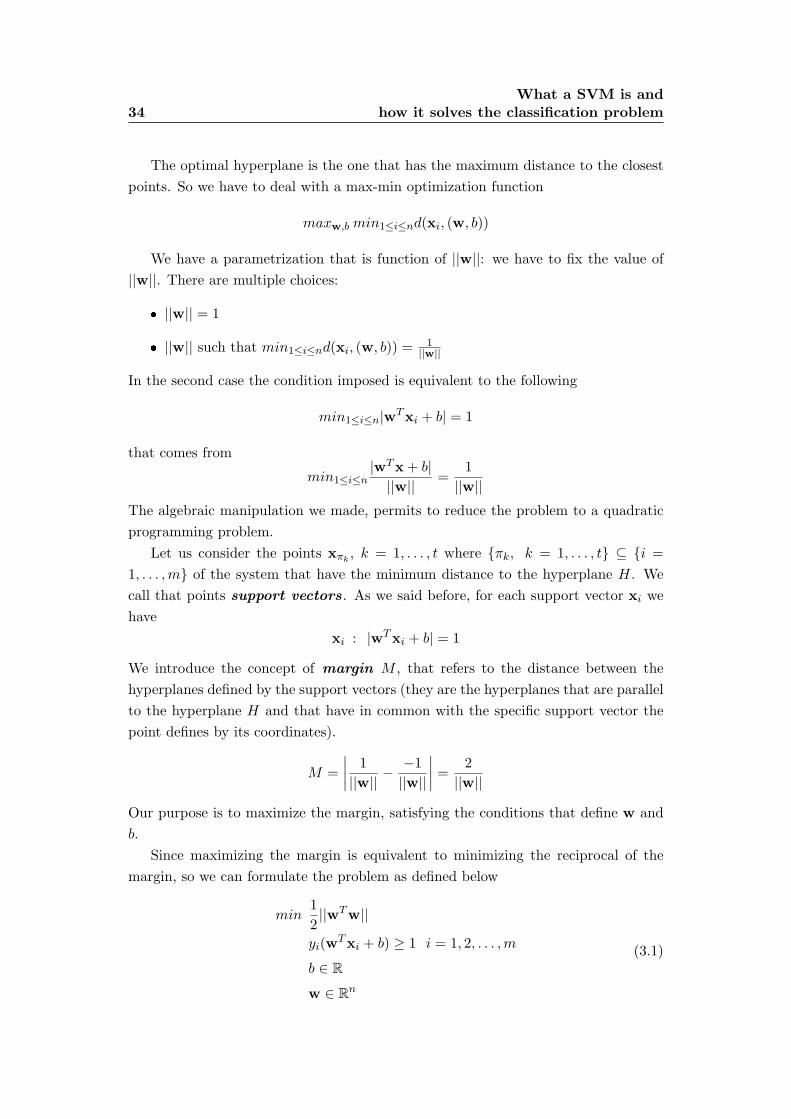
The optimal hyperplane is the one that has the maximum distance to the closest
points. So we have to deal with a max-min optimization function
maxw,b min1≤i≤nd(xi, (w, b))
We have a parametrization that is function of ||w||: we have to fix the value of
||w||. There are multiple choices:
� ||w|| = 1
� ||w|| such that min1≤i≤nd(xi, (w, b)) = 1||w||
In the second case the condition imposed is equivalent to the following
min1≤i≤n|wTxi + b| = 1
that comes from
min1≤i≤n|wTx+ b|
||w||=
1
||w||The algebraic manipulation we made, permits to reduce the problem to a quadratic
programming problem.
Let us consider the points xπk, k = 1, . . . , t where {πk, k = 1, . . . , t} ⊆ {i =
1, . . . ,m} of the system that have the minimum distance to the hyperplane H. We
call that points support vectors. As we said before, for each support vector xi we
have
xi : |wTxi + b| = 1
We introduce the concept of margin M , that refers to the distance between the
hyperplanes defined by the support vectors (they are the hyperplanes that are parallel
to the hyperplane H and that have in common with the specific support vector the
point defines by its coordinates).
M =
∣∣∣∣ 1
||w||− −1
||w||
∣∣∣∣ = 2
||w||
Our purpose is to maximize the margin, satisfying the conditions that define w and
b.
Since maximizing the margin is equivalent to minimizing the reciprocal of the
margin, so we can formulate the problem as defined below
min1
2||wTw||
yi(wTxi + b) ≥ 1 i = 1, 2, . . . ,m
b ∈ R
w ∈ Rn
(3.1)

3.3 How a SVM solves the classification problem 35
The Lagrangian relaxation of the given problem is
min1
2||w||2 −
m∑i=1
λi(yi(wTxi + b)− 1)
b ∈ R
w ∈ Rn
The solution of this relaxation is obtained applying the Karush-Kuhn-Tucker
(KKT) conditions to the problem in (3.1).
We recall them in the following [12]
Theorem [KKT conditions] :
Suppose that the objective function f : Rn → R and the constraint func-
tion gi : Rn → R are continuously differentiable at a point w∗.
Assume w∗ is a regular local minimum of a nonlinear programming prob-
lem.
Then there is a Lagrange multiplier vector Λ such that
∇f(w∗) =m∑i=1
λi∗∇gi(w
∗)
λi∗ ≥ 0 i = 1, . . . ,m
gi(w∗) ≥ 0 i = 1, . . . ,m
λi∗gi(w
∗) = 0 i = 1, . . . ,m
Note that
∇f(w∗) =
m∑i=1
λi∗∇gi(w
∗) ⇐⇒ ∇L(w, b,Λ) = 0
Necessary and sufficient conditions for
∇L(w, b,Λ) = 0
are
w∗ =
m∑i=1
yiλi∗xi
m∑i=1
yiλi∗ = 0

36What a SVM is and
how it solves the classification problem
The complete formulation of the Lagrangian relaxation is
min1
2||w||2 −
m∑i=1
λi(yi(wTxi + b)− 1)
m∑i=1
λiyi = 0
λi ≥ 0 i = 1, . . . ,m
b ∈ R
w ∈ Rn
The objective function can be properly manipulated, using the necessary and
sufficient conditions previously obtained. That is, knowing that the hyperplanes can
be written as linear combinations of the vectors of the training set (w =∑m
i=1 λiyixi)
and using the second condition that implies that∑m
i=1 λiyib = 0.
min
[1
2||w||2 −
m∑i=1
λi(yi(wTxi + b)− 1)
]=
= min
12
m∑i=1
λixiyi
m∑j=1
λjxjyj −m∑i=1
λixiyi
m∑j=1
λjxjyj −m∑i=1
λiyib+
m∑i=1
λi
=
= min
−1
2
m∑i=1
λixiyi
m∑j=1
λjxjyj +
m∑i=1
λi
The Lagrangian relaxation has to be minimized on w and b and to be maximized
on Λ.
So we can formulate the problem as in the following
maxΛ
m∑i=1
λi −1
2
m∑i,j=1
λiλjyiyjxixj
m∑i=1
λiyi = 0
λi ≥ 0 i = 1, . . . ,m
In the model above the bounds on w and b are replaced by bounds on the Lagrangian
multipliers and the training set vectors appear only as inner products between vectors.
Since the equation of the optimal hyperplane can be written as a linear combina-
tion of the vectors of the training set
w∗ =∑i
λ∗i yixi = Λ∗y x
Then
w∗x+ b = Λ∗y x · x+ b
3.3 How a SVM solves the classification problem 37
So the classifier is given by
sign
[m∑i=1
yiλ∗i (x · xi) + b∗
]
where we can find the value of b∗ from the following conditions
λ∗i (yi(w
∗x+ b∗)− 1) = 0 i = 1, . . . ,m
−→ b∗ = yi −w∗ · xi
Eventually, it is possible to demonstrate that [13]
b∗ = −1
2
[maxyi=−1w
∗Txi +minyi=+1w∗Txi
]In the solution, the points that have the correspondent Lagrangian multipliers λi > 0
are the support vectors; the other points of the training set have the correspondent
λi = 0 and so they do not influence the classifier (we could consider just the support
vectors’ points – the whole information about the training set is contained in those
points).
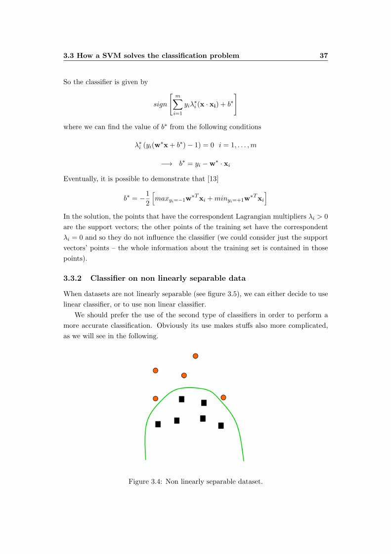
3.3.2 Classifier on non linearly separable data
When datasets are not linearly separable (see figure 3.5), we can either decide to use
linear classifier, or to use non linear classifier.
We should prefer the use of the second type of classifiers in order to perform a
more accurate classification. Obviously its use makes stuffs also more complicated,
as we will see in the following.
Figure 3.4: Non linearly separable dataset.

38What a SVM is and
how it solves the classification problem
3.3.2.1 Linear classifier on non linearly separable data
The linear classifier described above cannot deal with dataset that are non linearly
separable.
However it is possible to use a linear classifier (see figure 3.5) also on this kind of
data: we just have to relax the classification bounds, tolerating a certain number of
errors.
Figure 3.5: Non linearly separable dataset with a linear separation.
The optimum hyperplane is again determined by the support vectors points, but
there are some points that do not satisfy the condition yi(wTxi + b) ≥ 1. A possible
solution is to add some slack variables.
The new bounds are
yi(wTxi + b) ≥ 1− ξi i = 1, . . . ,m
ξi ≥ 0 i = 1, . . . ,m
b ∈ R
w ∈ Rn
where ξi > 1 represents the error that occurs.
We can reformulate the problem with a model that tries at the same time to
minimize ||w|| and minimum number of errors (in the objective function there is a
term∑m
i=1 ξi that represents an upper bound on the number of errors on the training
3.3 How a SVM solves the classification problem 39
data).
min1
2||w||2 + C(
m∑i=1
ξi)k
yi(w · xi + b) ≥ 1− ξi i = 1, . . . ,m
ξi ≥ 0 i = 1, . . . ,m
b ∈ R
w ∈ Rn
where C and k are parameters that are related to the penalty that occurs in case of
an error, and typically is k = 1.
Recalling that w =∑m
i=1 λiyixi, an equivalent formulation of the primal problem
(for k = 1), which we used in our experimentation, is
min1
2
m∑i=1
m∑j=1
λiλjyiyjxixj + Cm∑i=1
ξi
yi
m∑j=1
λjyjxj · xi + b
≥ 1− ξi i = 1, . . . ,m
ξi ≥ 0 i = 1, . . . ,m
λi ≥ 0 i = 1, . . . ,m
b ∈ R
As in 3.3.1, the Lagrangian relaxation of the given problem is
min
[1
2||w||2 + C(
m∑i=1
ξi)k −
m∑i=1
λi(yi(wTxi + b)− 1 + ξi)−
m∑i=1
γiξi
]
Under the following constraint, obtained applying KKT conditions to the problem
formulationm∑i=1
λiyi = 0
and
ξi ≥ 0 i = 1, . . . ,m
λi ≥ 0 i = 1, . . . ,m
b ∈ R
w ∈ Rn
The objective function can be properly manipulated, using the necessary and
sufficient conditions previously obtained. That is, knowing that the hyperplanes can

40What a SVM is and
how it solves the classification problem
be written as linear combinations of the vectors of the training set (w =∑m
i=1 λiyixi)
and using the condition∑m
i=1 λiyi = 0 that implies that∑m
i=1 λiyib = 0.
min
[1
2||w||2 + C(
l∑i=1
ξi)k −
m∑i=1
λi(yi(wTxi + b)− 1 + ξi)−
m∑i=1
γiξi
]=
= min
12
m∑i=1
λixiyi
m∑j=1
λjxjyj + C
m∑i=1
ξi −m∑i=1
λixiyi
m∑j=1
λjxjyj +
m∑i=1
λi −m∑i=1
λiξi +
m∑i=1
γiξi
=
= min
−1
2
m∑i=1
λixiyi
m∑j=1
λjxjyj +
m∑i=1
λi +
m∑i=1
(C − λi − γi)ξi
It is possible to demonstrate that
∑mi=1(C − λi − γi)ξi = 0.
The Lagrangian relaxation has to be minimized on w and b and to be maximized
on λ.
So we can formulate the problem as in the following
maxλ
m∑i=1
λi −1
2
m∑i,j=1
λiλjyiyjxixj
m∑i=1
λiyi = 0
0 ≤ λi ≤ C i = 1, . . . ,m
And, as in 3.3.1, the classifier is given by
sign
[m∑i=1
yiλ∗i (x · xi) + b∗
]
3.3.2.2 Non linear classifier on non linearly separable data
Another possibility to deal with non linearly separable data is to use a non linear
classifier.
The idea behind this approach is to create a sort of “lifting” (using a function Φ)
of the non linearly separable data on a new space (generally having more dimensions
than the previous one) where they are become linearly separable.
Φ : Rn 7→ RN N ≫ n
x 7→ Φ(x)
Through this procedure (known in the literature as kernel trick [14]) we can use once
again a linear classifier in the new space, as seen before.

3.3 How a SVM solves the classification problem 41
Figure 3.6: The SVM trick for non linearly separable data.
The previous equation for the classifier
sign
[m∑i=1
yiλ∗i (x · xi) + b∗
]
is changed in the following equation
sign
[m∑i=1
yiλ∗i (Φ(x) · Φ(xi)) + b∗
]
That model has a limit: the product Φ(x)·Φ(xi) involves high dimensional vectors.
A solution here is to introduce a kernel function of the form
K : Rn × Rn 7→ R
that substitutes the product K(xi,xj) = Φ(xi) · Φ(xj).
The characteristics and properties of the kernel function are defined by
Mercer Theorem :
A symmetric function K(xi,xj) is a kernel
if and only if
for any sample S = {x1, . . . ,xm}, the kernel matrix for S is positive
semi-definite.
Using the definition of the kernel function in the classifier we have
sign
[m∑i=1
yiλ∗iK(x,xi) + b∗
]
42What a SVM is and
how it solves the classification problem
And in the model
max
m∑i=1
λi −1
2
m∑i,j=1
λiλjyiyjK(xi,xj)
m∑i=1
λiyi = 0
0 ≤ λi ≤ C i = 1, . . . ,m
Or equivalently for the primal problem
min1
2
m∑i=1
m∑j=1
λiλjyiyjK(xi,xj) + Cm∑i=1
ξi
yi
m∑j=1
λjyjK(xi,xj) + b
≥ 1− ξi i = 1, . . . ,m
ξi ≥ 0 i = 1, . . . ,m
λi ≥ 0 i = 1, . . . ,m
b ∈ R
How to choose the kernel function?
Kernel methods work:
� mapping items on a different vectorial space;
� looking for linear relationships between items in that space.
Here there are several possibilities for the kernel method:
Linear:
K(xi,xj) =m∑k=1
(xi)k · (xj)k
Polynomial:
K(xi,xj) =
(1 +
m∑k=1
(xi)k · (xj)k
)d
Radial Based function:
K(xi,xj) = e−∑m
k=1((xi)k−(xj)k)2
2σ2
Gaussian:
K(xi,xj) = e−γ[∑m
k=1((xi)k−(xj)k)2] = e−γ||xi−xj ||2

3.3 How a SVM solves the classification problem 43
Multi-Layer Perceptron:
K(xi,xj) = tanh
[b
(m∑k=1
(xi)k(xj)k
)− c
]
However, there are not limits to the choice of the kernel function; necessary and
sufficient condition is that, since that functions have to represent an inner product in
the extended space, kernel functions satisfy the following properties:
1. K(x1,x2) = K(x2,x1)
2. K(x1,x2 + x3) = K(x1,x2) +K(x1,x3)
3. K(x1, αx2) = αK(x1,x2)
The most used kernel is the Gaussian one. It is different from the other types of
kernel because of its meaning: it represents a function whose value, given two points
in input, depends only on the distance between them, without any dependency on
the absolute position of the points in the whole set of points.
To understand the meaning and behaviour of Gaussian kernel, let us consider two
points in the original space: xi and xj .
� If the two points coincide, then d(xi,xj) = 0, then K(xi,xj) = 1;
� If not, the trend of K is strictly decreasing in the amount of distance (the
function trend is given in figure 3.7, where the x-axis represents the distance
and the y-axis the value of K, for Gaussian kernel).
An analogy to figure with Gaussian kernel.
To go deeply inside an intuitive comprehension of the behaviour of Gaussian kernel,
a useful analogy can be given.
Each point x of the training set is like a communication source that transmits a
particular signal f(x) uniquely associated to it, namely the constant signal +1 or −1.
This signal is manipulated externally (this is the contribution of the Gaussian kernel)
so that, after its emission, it is decreased with an exponential law, depending on the
distance (far from the transmitting point, the signal is close to 0, near the point the
signal is close to 1).
When we want to classify a new point x1, not belonging to the training set, we
perform the following actions: standing in x1, we measure the whole perceived signals,
computing the total signed sum: if the result is positive, then x1 is classify as a point
that belongs to class +1, otherwise if the result is negative x1 belongs to −1.

44What a SVM is and
how it solves the classification problem
Figure 3.7: Gaussian kernel value vs distance, for the parameter γ = 0.1, 1, 10, 100.
Clearly, the density of the training set points is strictly related to the determina-
tion of the constant (the value of γ in the exponential Gaussian function) that defines
the decay of the signal with the distance: if points are close together, then signals
can decrease in a less intense way than in the case they are far each from the others
(in this last case, if signals decrease too quickly there is the risk that the points do
not get any signal from the others).

3.3 How a SVM solves the classification problem 45
Figure 3.8: Signals analogy.

46What a SVM is and
how it solves the classification problem

Chapter 4
Alternative training models
4.1 Gaussian kernel models
In this section we will describe the mathematical models we implemented as alter-
native approaches to the classical quadratic programming model used by the SVM
approach, namely:
min1
2
m∑i=1
m∑j=1
λiλjyiyjK(xi,xj) + Cm∑i=1
ξi
yi
(m∑j=1
λjyjK(xi,xj) + b
)≥ 1− ξi i = 1, . . . ,m
ξi ≥ 0 i = 1, . . . ,m
λi ≥ 0 i = 1, . . . ,m
b ∈ R
(4.1)
where K(xj ,xi) is the considered kernel, e.g. the Gaussian one
K(xi,xj) = e−γ||xi−xj ||2
We recall that the resolution of the proper mathematical model enables a SVM
to determinate the optimum Λ and b parameters to be used in phase of classification.
The aforesaid model is structured on the training set points.
About the models that will be proposed in the following, we also recall that
A MIP problem (Mixed Integer Programming) consists in the minimiza-
tion of a linear objective function with a finite number of linear con-
straints, with an additional constraint that requires some/all variables to
be integer [26].
48 Alternative training models
This kind of models have to be solved with proper CPLEX settings. In the .dat file,
where we define the parameters setting to be read by CPLEX before the optimization,
we have the following “rules”:
set mip tolerance integer 0
set mip timelimit 1200
set mip polishaftertime 900
where:
� the first line refers to the tolerance considered by the solver on the constrains;
� the second line sets a timelimit of 20 minutes for the optimization process;
� the third line establishes to start a proper procedure, called polish, after the
passage of 34 of the timelimit interval.
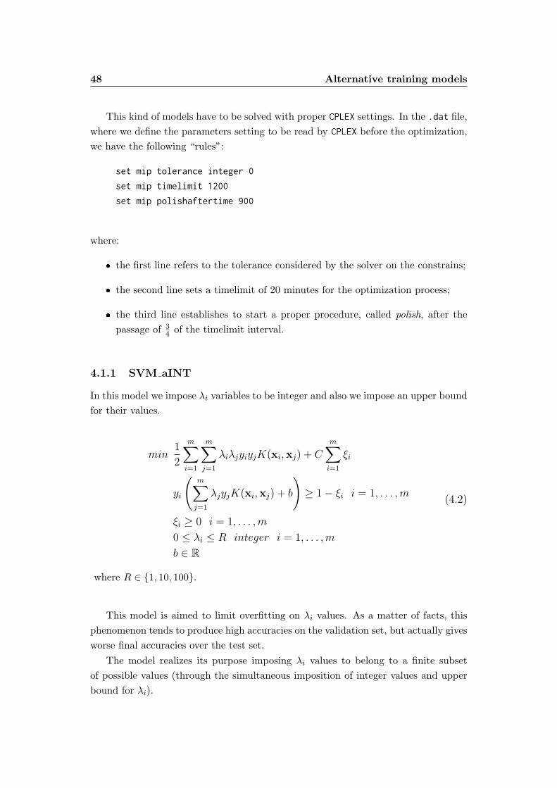
4.1.1 SVM aINT
In this model we impose λi variables to be integer and also we impose an upper bound
for their values.
min1
2
m∑i=1
m∑j=1
λiλjyiyjK(xi,xj) + Cm∑i=1
ξi
yi
(m∑j=1
λjyjK(xi,xj) + b
)≥ 1− ξi i = 1, . . . ,m
ξi ≥ 0 i = 1, . . . ,m
0 ≤ λi ≤ R integer i = 1, . . . ,m
b ∈ R
(4.2)
where R ∈ {1, 10, 100}.
This model is aimed to limit overfitting on λi values. As a matter of facts, this
phenomenon tends to produce high accuracies on the validation set, but actually gives
worse final accuracies over the test set.
The model realizes its purpose imposing λi values to belong to a finite subset
of possible values (through the simultaneous imposition of integer values and upper
bound for λi).
4.1 Gaussian kernel models 49
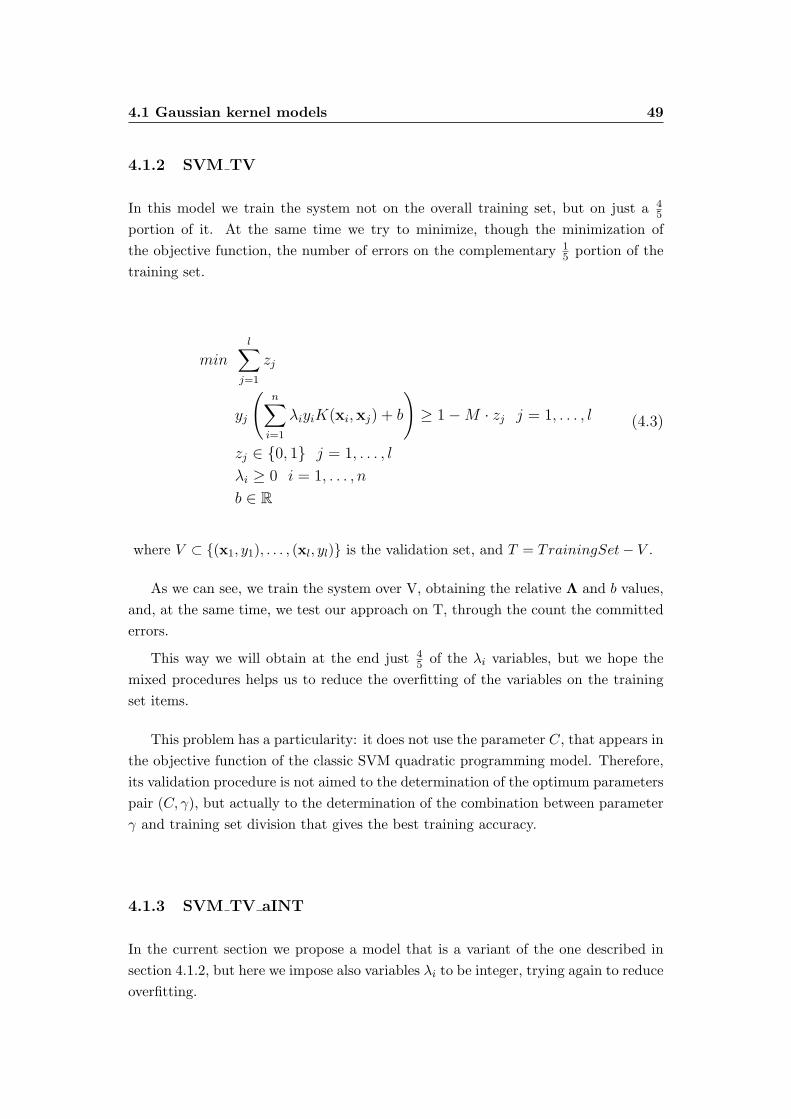
4.1.2 SVM TV
In this model we train the system not on the overall training set, but on just a 45
portion of it. At the same time we try to minimize, though the minimization of
the objective function, the number of errors on the complementary 15 portion of the
training set.
minl∑
j=1
zj
yj
(n∑
i=1
λiyiK(xi,xj) + b
)≥ 1−M · zj j = 1, . . . , l
zj ∈ {0, 1} j = 1, . . . , l
λi ≥ 0 i = 1, . . . , n
b ∈ R
(4.3)
where V ⊂ {(x1, y1), . . . , (xl, yl)} is the validation set, and T = TrainingSet− V .
As we can see, we train the system over V, obtaining the relative Λ and b values,
and, at the same time, we test our approach on T, through the count the committed
errors.
This way we will obtain at the end just 45 of the λi variables, but we hope the
mixed procedures helps us to reduce the overfitting of the variables on the training
set items.
This problem has a particularity: it does not use the parameter C, that appears in
the objective function of the classic SVM quadratic programming model. Therefore,
its validation procedure is not aimed to the determination of the optimum parameters
pair (C, γ), but actually to the determination of the combination between parameter
γ and training set division that gives the best training accuracy.
4.1.3 SVM TV aINT
In the current section we propose a model that is a variant of the one described in
section 4.1.2, but here we impose also variables λi to be integer, trying again to reduce
overfitting.

50 Alternative training models
minm∑j=1
zj
yj
(n∑
i=1
λiyiK(xi,xj) + b
)≥ 1−M · zj j = 1, . . . ,m
zj ∈ {0, 1} j = 1, . . . ,m
0 ≤ λi ≤ R integer i = 1, . . . ,m
b ∈ R
(4.4)
The same consideration made previously for the characteristics of SVM TV model
are valid also for this model. In addiction, the restricted possible values imposed for
variables λi represent a further attempt to the reduction of overfitting.
4.1.4 SVM aAll TV
This is the same model as in section 4.1.2, but, in this case, we use all the variables
λk in the final classifier, integrating the missing λj (those that were not determined
by the resolution of the model) with the mean value calculated on the given λi.
With this model we want to improve the performances of SVM TV using more
variables than those used by the aforesaid model.
4.1.5 SVM Mixed
In this model we accept to incur in a number of errors during the classification of the
training items that is at most equal to a certain percentage of the total number of
training items themselves.
min1
2
m∑i=1
m∑j=1
λiλjyiyjK(xi,xj)
yi
(m∑j=1
λjyjK(xj,xi)
)≥ 1−M · zi i = 1, . . . ,m
m∑i=1
zi ≤ C ·m
zi ∈ {0, 1} i = 1, . . . ,m
λi ≥ 0 i = 1, . . . ,m
(4.5)
where C ∈ {1, 10}.
4.1 Gaussian kernel models 51
With this model we want again to reduce the overfitting phenomenon on the
training set. We aim to do that through the action of the constraint that enables the
system to commit a number of errors that is even higher than the number commit-
ted by the classic SVM approach model. This action reduces the accuracies on the
validation set, that is it makes the variables less fitting to the validation set itself.
Besides, another interesting observation is that we try to minimize the total mis-
classification not through the minimization of the sum of ξi variables, but yet through
the minimization of the number of misclassified points (represented by zi variables).
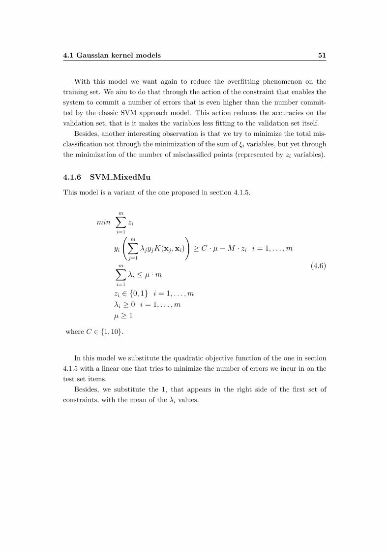
4.1.6 SVM MixedMu
This model is a variant of the one proposed in section 4.1.5.
min
m∑i=1
zi
yi
(m∑j=1
λjyjK(xj,xi)
)≥ C · µ−M · zi i = 1, . . . ,m
m∑i=1
λi ≤ µ ·m
zi ∈ {0, 1} i = 1, . . . ,m
λi ≥ 0 i = 1, . . . ,m
µ ≥ 1
(4.6)
where C ∈ {1, 10}.
In this model we substitute the quadratic objective function of the one in section
4.1.5 with a linear one that tries to minimize the number of errors we incur in on the
test set items.
Besides, we substitute the 1, that appears in the right side of the first set of
constraints, with the mean of the λi values.

52 Alternative training models
4.2 Linear kernel models
In this section we will describe models that are intended to use the linear kernel.
Hence, they are expressed in terms of (w, b), instead of Λ and b.
4.2.1 SVM K-lin
This is the classical quadratic programming problem, using linear kernel.
min1
2||w||2 +
m∑i=1
ξi
yi(wTxi + b) ≥ 1− ξi i = 1, . . . ,m
ξi ≥ 0 i = 1, . . . ,m
w ∈ Rn
b ∈ R
(4.7)
As we can see, the kernel function does not appear in the usual formulationK(xi,xj), where
K(xi,xj) =
m∑k=1
(xi)k · (xj)k
but instead, it is intrinsic in the use of the hyperplane formulation
w =
m∑i=1
λiyixi
4.2.2 SVM K-lin wINT
This model is similar to the one proposed in section 4.2.1, but here we also impose
w to be an integer vector.
min1
2 · S2||w||2 +
m∑i=1
ξi
yi(1
SwTxi + b) ≥ 1− ξi i = 1, . . . ,m
ξi ≥ 0 i = 1, . . . ,m
w ∈ Zn
b ∈ R
(4.8)
where S ∈ {1, 10, 100, 1000} is a scaling factor.

4.2 Linear kernel models 53
With this model we want to limit the possible values to be assumed by w vector’s
components.
Our guess here is that we risk much more overfitting permitting w to belong to
Rn instead of imposing w (or 10w, or 100w, or 1000w) to belong to Zn.

54 Alternative training models

Chapter 5
Experimental tests and results
5.1 Real world datasets
All the datasets used in our experimentation were downloaded from UCI Machine
Learning Repository [21].
The UCI Machine Learning Repository is a collection of databases, domain the-
ories, and data generators that are used by the machine learning community for the
empirical analysis of machine learning algorithms. The archive was created as an ftp
archive in 1987 by David Aha and fellow graduate students at UC Irvine. Since then,
it has been widely used by students, educators, and researchers all over the world as
a primary source of machine learning data sets.
We decided to test our approaches on eleven datasets, the same ones that also
J.P. Brooks used in his work about classification [22].
The chosen datasets contain numerical (real or integer) and categorical (numerical
and literal) attributes, and just two possible classes for each item. In other words
they are perfectly suitable for binary classification through SVM and other similar
approaches.
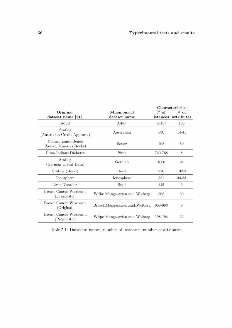
In table 5.1 we have a summary description of the datasets used in the experi-
mental tests: their name from the repository, their label (used by Brooks), number
of instances, and number of features.
5.1.1 Preprocessing on raw data
Data from UCI Repository is not immediately suitable for testing our classification
methods.
As Brooks suggests, before their use data has to be properly preprocessed and
normalized.
1Before-after preprocessing and normalization of the dataset.
56 Experimental tests and results
Characteristics1
Original Mnemonical # of # ofdataset name [21] dataset name istances attributes
Adult Adult 30157 105
StatlogAustralian 690 14-41
(Australian Credit Approval)
Connectionist BenchSonar 208 60
(Sonar, Mines vs Rocks)
Pima Indians Diabetes Pima 769-768 8
StatlogGerman 1000 24
(German Credit Data)
Statlog (Heart) Heart 270 13-23
Ionosphere Ionosphere 351 34-33
Liver Disorders Bupa 345 6
Breast Cancer WisconsinWdbc Mangasarian and Wolberg 568 30
(Diagnostic)
Breast Cancer WisconsinBreast Mangasarian and Wolberg 699-683 9
(Original)
Breast Cancer WisconsinWdpc Mangasarian and Wolberg 198-194 33
(Prognostic)
Table 5.1: Datasets: names, number of instances, number of attributes.

5.1 Real world datasets 57
In the following we describe the procedure to be performed on raw data to prepare
the input to our classification procedures.
Removing missing values
If there are items with one or more missing values, those items are removed from
the relative dataset.
Most of the times, missing attributes are indicated, in the UCI Repository, with
a ’?’, or a ’-’.
Converting categorical attributes
If an attribute is of categorical type, that can assume k possible values, it is replaced
by k attributes which can attain just 2 possible values (generally 0 or 1).
Example:
If there is an attribute size, that has values ∈ {small,medium, large}, itis replaced by 3 attributes: size 1, size 2 and size 3 that have all values
∈ {0, 1}.
size ∈ {small,medium, large}
. . . size . . .
. . . large . . .
. . . . . . . . .
. . . size1 size2 size3 . . .
. . . 0 0 1 . . .
. . . . . . . . . . . . . . .
Converting literal attributes
If an attribute is a literal one, that can attain literal values within a finite set of
words of cardinality k, it is conceptually treated as a categorical attribute, so it is
replaced by k binary attributes.
Calculating mean value and standard deviation
For each attribute in the dataset, mean value and standard deviation are computed
on the training set.
Normalizing the dataset values
First of all, attributes that have standard deviation that is zero are removed from
the relative datasets.
Secondly, each attribute value is normalized by subtracting the mean value and
dividing by the standard deviation, both calculated, as seen above, on the training
set items only.
58 Experimental tests and results
5.1.2 Experimental choices for data training
In order to perform our experiments, each dataset is randomly partitioned in such
a way that the 70% of the items belong to the training set, and the remaining 30%
to the test set. This last part of the dataset is taken away at the beginning, and is
never used during the whole training procedure: it is used just at the end, during the
computation of the final accuracy (the accuracy on the test set) that permits us to
evaluate the goodness of the considered approach.
The training part of the dataset is, in turn, divided into 5 parts to perform 5-fold
cross validation. This procedure is necessary to choose the optimal parameters to
train the system and use the classifier on the test set.
Since our experimental tests require the subsequent resolution of several optimiza-
tion problems, some of them require a resolution time of about twenty minutes, we
decided to restrict in most cases out analysis to nine of the eleven datasets that have
less then 800 items. So, for the experimentations described in section 4, we excluded
the use of “Adult” and “German” datasets.
5.1.3 Availability of the data on the web
As we said previously, the datasets used, which where taken from the UCI Machine
Learning Repository, contain raw data that are inhomogeneous.
Since the programming effort to create a proper parser for each dataset, in order
to extract the ordered non zero features and the classes, was not trivial, we thought
that it could be useful to make available on the web the postprocessed datasets.
The format we chose is the SVMlight format, described in 6.1.2.2, for not nor-
malized dataset items, with categorical and literal attributes converted to numerical
ones.
The eleven datasets used can be found at the link
www.dei.unipd.it/˜fisch/datasetSVM.tar.gz
altogether in a single compressed folder.

5.2 Comparison betweenSVM approach and A1B0 approach 59
5.2 Comparison betweenSVM approach and A1B0 approach
In the following we report an analysis about the advantage, in term of accuracy, of a
classification based on the classic SVM approach (with Gaussian kernel) without any
kind of training procedure, just applying the final classifier (sign[∑m
i=1 yiλiK(x, xi)+
b] – with λi = 1 ∀i, and b = 0).
5.2.1 A1B0 approach
This approach just sets
λi = 1 ∀i = 1, . . . ,m
b = 0
so that the classifier becomes:
sign
[m∑i=1
yiK(xi, xj)
](5.1)
where
K(xi,xj) = e−γ||xi−xj ||2
We want to remark the fact that the use of A1B0 approach allows to realize a
classification without performing any kind of training procedure on data. For this
reason, A1B0 approach is much less computationally expensive than SVM approach,
and also not subject to overtuning.
5.2.2 Parameters setting: γ = 0.1
SVM approach
In the comparison in analysis only one parameter is free and can be set offline.
Namely parameter γ in the Gaussian kernel.
In our experimentation, according to [22], we performed our tests on just few
values of γ, i.e.
γ ∈ {0.1, 1, 10, 100, 1000}
As we could experiment in the very numerous tests, in more than the 90% of the
cases, the highest accuracies are obtained using γ = 0.1.
That is the reason why we decided to restrict the interest of this comparison to
the use of this value for γ.
For the value of parameter C, we decided to leave the choice to the software used
for the computation of the 50 accuracies of SVM approach, that is to SVMlight .

60 Experimental tests and results
The default value used is [20]
C = [avg. x · x]−1
that is, the reciprocal of the average of the feature vectors inner products is the value
assigned to C.
5.2.3 Organization of the tests
First of all we have to sample randomly each datasets, in order to obtain what we
call an instance of a dataset.
A single instance of a dataset consists in the random division of the dataset itself
in training set (portion of 710 of the dataset) and complementary test set.
We produce 50 different instances for each dataset.
Then, in parallel, we obtain, for each of the aforesaid instances:
� The accuracy with SVM approach;
� The accuracy with A1B0 approach.
We produced 50 couples of accuracies, where the first element of the couple is
obtained with SVM approach and the second with A1B0 approach.
We can consider each couple as a couple of “measurements” produced by two dif-
ferent “instruments” on the same data – in our case the instrument is the classification
procedure used.
We want to:
� Understand, with a rigorous analysis, if the two instruments have a statistically
significative difference, or if they are statistically comparable.
� Perform a statistical analysis and comparison of the two methods.
The first evaluation can be done through the use of a statistical method known
as Wilcoxon test, described in detail in Appendix B.
The second aim can be reached by computing some statistical indicators like
mean and standard deviation of the accuracies given by SVM approach and by A1B0
approach, percentage of SVM approach and A1B0 approach wins, mean and standard
deviation of Λ parameters sparsity for SVM approach. These indicators enable us to
understand if the use of a SVM is really always useful and advantageous in place of
the use of a much simpler and computationally inexpensive method like the classifier
in equation (5.1).

5.3 Experimental results for tests described in section 5.2 61
5.3 Experimental results for tests described in section5.2
In this section we will give a global evaluation of the results of the tests described in
section 5.2.
5.3.1 Statistical significance of the difference betweenthe two methods
As previously said, we used Wilcoxon test (presented and described in Appendix B,
to evaluate if there is a statistically significative difference between SVM approach
and A1B0 approach for the classification of the same test set items.
We perform the test using the statistical software R; for details about its installa-
tion and use see 6.1.4.
In the following the evaluation of the results and some considerations about them.
Dataset p-valueAdult < 0.001
Australian 0.0051Breast Mangasarian and Wolberg < 0.001
Bupa < 0.001German < 0.001Heart < 0.001
Ionosphere < 0.001Pima < 0.001Sonar < 0.001
Wdbc Mansagarian and Wolberg < 0.001Wpbc Mangasarian and Wolberg 0.0038
Table 5.2: p-values for comparison between SVM approach and A1B0 approach.
In table 5.3.1 we can see the p-values obtained comparing, through the use of
Wilcoxon test technique, 50 couples of measurements, computed respectively with
SVM approach and A1B0 approach.
As we can see, for all the eleven datasets used in our experimentation, we have
p− value < 0.01
That is, we can state that:
SVM approach is statistically different from A1B0 approach with a level
of confidence greater than the 99%.
This result could not seem to be very interesting. Considering all the theory
and the scientific research about all the possible settings (parameters settings, kernel

62 Experimental tests and results
choices, . . . ) of Support Vector Machines, we could imagine that SVM approach
would be always preferable, in terms of accuracy gain, to A1B0 approach.
But the results of a statistical analysis and comparison between the two ap-
proaches are rather surprising.
5.3.2 Some statistical considerations about the comparison ofthe two methods
In the following we will evaluate the results for the tests in analysis at two different
levels:
� At the level of each single dataset;
� At a high global level comprehensive of all the used datasets.
For the results in detail, at the level of each of the 50 instances taken from each
of the eleven datasets, we refer to Appendix A.
5.3.2.1 Datasets level
A global vision of those results at the level of each dataset is given in table 5.32.
Dataset µSVM µA1B0 σSVM σA1B0 SVM> A1B0> µspars σsparsAdult 81.79 75.11 0.39 0.38 100.00 0.00 35.99 0.28
Australian 82.78 83.69 2.74 2.51 30.00 70.00 15.51 0.42
Breast Mangasarian and Wolberg 96.84 90.27 0.91 1.97 100.00 0.00 85.15 1.08
Bupa 70.52 58.73 3.90 4.11 98.00 0.00 20.51 2.25
German 72.03 70.03 2.48 2.36 100.00 0.00 23.03 1.56
Heart 79.80 81.78 3.67 4.04 28.00 62.00 21.52 2.12
Ionosphere 93.96 73.28 2.14 4.59 100.00 0.00 41.12 1.99
Pima 75.80 65.83 2.20 3.13 100.00 0.00 42.82 1.86
Sonar 59.59 83.49 7.06 5.15 0.00 100.00 0.61 0.50
Wdbc Mangasarian and Wolberg 95.49 92.68 1.88 2.51 86.00 12.00 55.09 1.04
Wpbc Mangasarian and Wolberg 75.09 75.93 5.06 5.04 16.00 48.00 9.65 2.44
Table 5.3: Results for each dataset for comparison SVM vs A1B0.
Where:
� µSVM is the mean calculated on the accuracies obtained from SVM approach;
� µA1B0 is the mean calculated on the accuracies obtained from A1B0 approach;
� σSVM is the standard deviation calculated on the accuracies obtained from SVM
approach;
2In yellow we marked where the SVM approach wins, in green where the A1B0 approach wins.

5.3 Experimental results for tests described in section 5.2 63
� σA1B0 is the standard deviation calculated on the accuracies obtained from
A1B0 approach;
� SVM> is the percentage of wins of SVM approach (percentage of times theaccuracy obtained with SVM approach is strictly greater than the one obtainedwith A1B0 approach on the same instance);
� A1B0> is the percentage of wins of A1B0 approach (percentage of times theaccuracy obtained with A1B0 approach is strictly greater than the one obtainedwith SVM approach on the same instance);
� µspars is the average sparsity (number of zero component of the vector Λ) ofSVM approach;
� σspars is the sparsity standard deviation of SVM approach.
As we can see, differently from our expectations, the SVM approach does not lead
always to produce higher accuracies than A1B0 approach. Actually, in four cases out
of eleven, the simpler and computationally inexpensive A1B0 approach gives better
accuracies than the competitor.
Another interesting observation concerns the values computed for the sparsity of
SVM approach. The claim of SVM theory is that its approach enables to determine Λ
vectors characterized by a high sparsity. This property is quite important and useful
because it ensures to decrease the overfitting effect in classification: sparse Λ vectors
permits to identify a few points (the so-called support vectors) of the training set that
really give useful information for the classification of new points (those belonging
to the test set), while removing all the other points that, in the final process of
classification, could give a misleading information (for example, because they are
outliers in the training points system).
Recalling that our analysis is restricted to the use of the Gaussian kernel, with pa-
rameter γ = 0.1, we can observe that actually, except for dataset Breast Mangasarian
and Wolberg, sparsity of SVM approach is not so relevant.
Furthermore, we can observe that, even in the rare cases where the mean sparsity
reaches the 50%, this does not have a relevant impact that enables to realize a con-
siderable gain in term of accuracy. In addiction, that these values for sparsity do not
affect the use of the SVM with a really sensible reduction of memory use and overall
speed of the SVM computations.
5.3.2.2 Higher global level
For an overview of the results at a higher level, we can consider altogether the eleven
datasets; the related indicators are given in table 5.4.
where, ad before:

64 Experimental tests and results
µSVM µA1B0 σSVM σA1B0 SVM> A1B0> µspars σspars
83.24 77.35 2.95 3.25 68.91 26.55 31.9 1.41
Table 5.4: Global results for comparison SVM vs A1B0.
� µSVM is the mean calculated on the accuracies obtained from SVM approach;
� µA1B0 is the mean calculated on the accuracies obtained from A1B0 approach;
� σSVM is the standard deviation calculated on the accuracies obtained from SVM
approach;
� σA1B0 is the standard deviation calculated on the accuracies obtained from
A1B0 approach;
� SVM> is the percentage of wins of SVM approach (percentage of times theaccuracy obtained with SVM approach is strictly greater than the one obtainedwith A1B0 approach on the same instance);
� A1B0> is the percentage of wins of A1B0 approach (percentage of times theaccuracy obtained with A1B0 approach is strictly greater than the one obtainedwith SVM approach on the same instance);
� µspars is the mean calculated on the sparsity (number of zero component of thevector Λ) of SVM approach;
� σspars is the sparsity standard deviation of SVM approach.
Before any analysis of those data, it is fundamental to make an important con-
sideration. The percentage results in table 5.4 are much less significative than the
results in table 5.3, because the first give overall statistical information about data
whose nature is “clustered”. As a matter of fact, considering altogether the eleven
datasets, we deal with data showing a quite high similarity within a single dataset,
and a quite high dissimilarity between a dataset and another one. In other words, in
this case, data are highly inhomogeneous.
However, as we can see, using SVM approach (that implies to solve a computa-
tionally expensive quadratic programming model), we can get an accuracy advantage
just of the 5.9% over the use of a much simpler approach based on the classifier in
equation (5.1).
Furthermore, the simpler approach is not always worse than the first one: about
27% times A1B0 approach wins giving higher accuracies, and 4-5% times it matches
the SVM one.
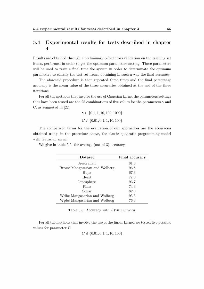
5.4 Experimental results for tests described in chapter 4 65
5.4 Experimental results for tests described in chapter4
Results are obtained through a preliminary 5-fold cross validation on the training set
items, performed in order to get the optimum parameters setting. These parameters
will be used to train a final time the system in order to determinate the optimum
parameters to classify the test set items, obtaining in such a way the final accuracy.
The aforesaid procedure is then repeated three times and the final percentage
accuracy is the mean value of the three accuracies obtained at the end of the three
iterations.
For all the methods that involve the use of Gaussian kernel the parameters settings
that have been tested are the 25 combinations of five values for the parameters γ and
C, as suggested in [22]
γ ∈ {0.1, 1, 10, 100, 1000}
C ∈ {0.01, 0.1, 1, 10, 100}
The comparison terms for the evaluation of our approaches are the accuracies
obtained using, in the procedure above, the classic quadratic programming model
with Gaussian kernel.
We give in table 5.5, the average (out of 3) accuracy.
Dataset Final accuracy
Australian 81.8Breast Mangasarian and Wolberg 96.8
Bupa 67.3Heart 77.0
Ionosphere 93.7Pima 74.3Sonar 82.0
Wdbc Mangasarian and Wolberg 95.5Wpbc Mangasarian and Wolberg 76.3
Table 5.5: Accuracy with SVM approach.
For all the methods that involve the use of the linear kernel, we tested five possible
values for parameter C
C ∈ {0.01, 0.1, 1, 10, 100}

66 Experimental tests and results
5.4.1 Results with Gaussian kernel
In the following we report the results we got training the system with classifiers ob-
tained by the alternative mathematical models previously described, all using Gaus-
sian kernel. We recall that the results in tables 5.7, 5.8, 5.9, 5.10, 5.11 and 5.12 have
to be compared with the ones in table 5.5.
Preliminary considerations
� Small values of γ, in general, give the highest accuracies (in our tests, optimum
parameters couples involve, in the 90% of the cases, by the value γ = 0.1). In
other words, high values of γ give scarce accuracies. Recalling the signal analogy
explained in figure 3.8, we have that the kernel function can be conceptually
associated to the power shape of the signal irradiated by each point in the space
around. A big value of γ implies that the kernel function acts like an impulse:
it is strong near the item point and much lower in the immediate vicinity of
the point itself. In this respect, a kernel function similar to an impulse (Dirac
delta), is associated to a classifier that is particularly able to categorize with
high accuracy a known point, that is, a point of the training set, instead of a
new and unknown point belonging to the test set.
� The values assumed by λi’s parameters, that we obtained from the resolution of
the classical quadratic programming problem with Gaussian kernel, differently
from what we imagined, have lots of decimal places, that is, tend to be very
fitting to items set in training set.
� Accuracies estimated during the repeated procedure of validation, as we could
imagine, are higher than the ones got during the final classification.
The analysis of the behaviour of the system confirm the overfitting phenomenon plays
a central role in the procedure.
The above considerations prompted us to plan, implement and test new alterna-
tive approaches that try to answer to the question “how can we try to contrast the
overfitting effect?”
We undertook the following possibilities:
� Trying to impose the choice of variables λi’s and b that have less degrees of
freedom than in the case of the classical problem – SVM aINT model ;
� Trying to impose that, during the validation phase, also a test procedure is
realized, in such a way to choose Λ and b parameters whose validity is already
tested on a items subset different from the training one – SVM TV models;

5.4 Experimental results for tests described in chapter 4 67
� Allowing the system for a certain number of misclassifications in the training
set, hoping that this makes the model less fitting to the specific training set
and produce more appropriated variables to be used by the final classifier –
SVM Mixed and MixedMu models.
Final considerations
The goodness of a classifier depends on:
1. The type of the chosen kernel;
2. The validity of the training model;
3. The validation procedure.
Now, we understood that the Gaussian kernel is a good and complete classifier by
itself, that is: it provides reasonable accuracies also without taking care to the other
two factors just enumerated.
Our claim is that the use of Gaussian kernel reduces the importance of the op-
timization problem, or makes it even counter-productive in some cases (because of
overfitting).
To further prove this thesis about the role of Gaussian kernel, we performed the
same tests for the evaluation of the superiority, in terms of accuracy, of SVM approach
towards A1B0 approach (see section 5.3), but this time using linear kernel. This way,
we could evaluate the behaviour of the linear kernel as a classifier by itself, compared
to the behaviour of the overall SVM approach that uses the same linear kernel to
perform the final classification over the test set.
We observed that linear kernel is not a so good classifier by itself as Gaussian
kernel is. Overall results, for tests performed on 50 instances for each of the eleven
datasets, are given in table 5.6. As we can see, the superiority of SVM approach
towards A1B0 approach, that for Gaussian kernel is 5.9%, for linear kernel increases
to 7.4%.
µSVM µA1B0 σSVM σA1B0 SVM> A1B0> µspars σspars
82.18 74.80 1.19 3.12 79.45 12.38 30.80 1.52
Table 5.6: Global results for comparison SVM vs A1B0 with linear kernel.

68 Experimental tests and results
SVM aINT
Dataset value of R Final accuracy
Australian1 81.510 79.7100 77.6
Breast Mangasarian and Wolberg1 96.910 96.2100 96.2
Bupa1 68.910 67.6100 67.0
Heart1 78.610 77.4100 76.7
Ionosphere1 94.010 93.4100 93.7
Pima1 73.010 74.3100 73.7
Sonar1 78.310 79.4100 81.5
Wdbc Mangasarian and Wolberg1 97.510 96.3100 96.3
Wpbc Mangasarian and Wolberg1 76.310 76.8100 76.8
Table 5.7: Accuracy with SVM aINT approach.

5.4 Experimental results for tests described in chapter 4 69
SVM TV aINT
Dataset value of R Final accuracy
Australian
1 77.010 77.6100 77.01000 77.6
Breast Mangasarian and Wolberg
1 97.110 96.7100 96.11000 96.7
Bupa
1 60.010 60.2100 60.21000 58.8
Heart
1 74.110 77.0100 76.71000 74.1
Ionosphere
1 92.810 92.8100 94.01000 90.7
Pima
1 67.610 68.4100 69.01000 68.4
Sonar
1 77.310 76.7100 77.31000 80.4
Wdbc Mangasarian and Wolberg
1 93.410 92.8100 93.41000 93.6
Wpbc Mangasarian and Wolberg
1 76.810 73.6100 73.61000 73.6
Table 5.8: Accuracy with SVM TV aINT approach.

70 Experimental tests and results
SVM TV
Dataset Final accuracy
Australian 79.9Breast Mangasarian and Wolberg 96.1
Bupa 66.4Heart 74.9
Ionosphere 93.1Pima 71.7Sonar 80.4
Wdbc Mangasarian and Wolberg 92.2Wpbc Mangasarian and Wolberg 76.8
Table 5.9: Accuracy with SVM TV approach.
SVM Mixed
Dataset C Final accuracy
Australian1 79.810 80.5
Breast Mangasarian and Wolberg - n.d.3
Bupa1 63.810 64.1
Heart1 76.710 77.0
Ionosphere1 87.710 87.7
Pima1 66.210 65.8
Sonar1 83.610 85.7
Wdbc Mangasarian and Wolberg1 97.510 97.5
Wpbc Mangasarian and Wolberg1 77.410 76.7
Table 5.10: Accuracy with SVM Mixed approach.
3CPLEX error in solving: Q matrix non semi-definite positive because of numericalissues.
4CPLEX error in solving: Q matrix non semi-definite positive because of numericalissues.

5.4 Experimental results for tests described in chapter 4 71
SVM aAll
Dataset Final accuracy
Australian 80.7Breast Mangasarian and Wolberg 94.6
Bupa 67.7Heart 78.2
Ionosphere 94.3Pima 70.6Sonar 83.1
Wdbc Mangasarian and Wolberg 94.3Wpbc Mangasarian and Wolberg 77.4
Table 5.11: Accuracy with SVM aAll TV approach.
SVM MixedMu
Dataset C Final accuracy
Australian1 78.410 78.4
Breast Mangasarian and Wolberg - n.d.4
Bupa1 63.810 64.4
Heart1 76.310 75.9
Ionosphere1 82.410 80.7
Pima1 71.610 72.9
Sonar1 82.010 82.0
Wdbc Mangasarian and Wolberg1 94.210 91.7
Wpbc Mangasarian and Wolberg1 76.310 76.7
Table 5.12: Accuracy with SVM MixedMu approach.
In table 5.13 we have the unified vision of all the results obtained with Gaussian
kernel.

72 Experimental tests and results
Globalresu
lts
Data
set
SVM
SVM
aIN
TSVM
TV
SVM
TV
aIN
TSVM
aAll
TV
SVM
Mixed
SVM
MixedM
uA1B0
Austra
lian
81.881.5
79.9
77.080.7
80.578.4
83.7
Bre
ast
96.896.9
96.1
97.194.6
––
90.3
Bupa
67.368.9
66.4
66.067.7
64.163.8
58.7
Heart
77.078.6
74.9
74.178.2
77.076.3
81.8
Ionosp
here
93.794.0
93.1
92.894.3
87.882.4
73.3
Pim
a74.3
73.0
71.1
67.670.6
65.871.6
65.8
Sonar
82.078.3
80.4
77.383.1
85.782.0
83.5
Wdbc
95.597.5
92.2
93.494.3
97.594.2
92.7
Wpbc
76.376.8
76.8
76.777.4
76.776.3
75.9
Table
5.13:Allob
tained
accu
racies,
with
Gaussian
kern
el.
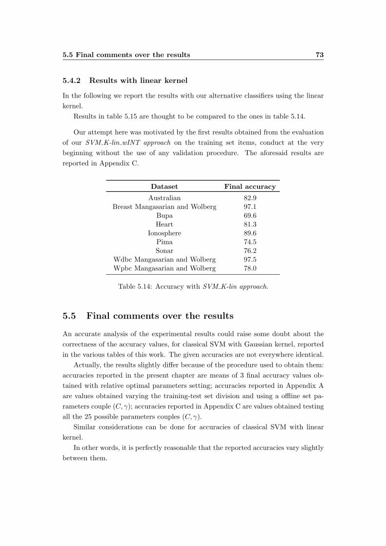
5.5 Final comments over the results 73
5.4.2 Results with linear kernel
In the following we report the results with our alternative classifiers using the linear
kernel.
Results in table 5.15 are thought to be compared to the ones in table 5.14.
Our attempt here was motivated by the first results obtained from the evaluation
of our SVM K-lin wINT approach on the training set items, conduct at the very
beginning without the use of any validation procedure. The aforesaid results are
reported in Appendix C.
Dataset Final accuracy
Australian 82.9Breast Mangasarian and Wolberg 97.1
Bupa 69.6Heart 81.3
Ionosphere 89.6Pima 74.5Sonar 76.2
Wdbc Mangasarian and Wolberg 97.5Wpbc Mangasarian and Wolberg 78.0
Table 5.14: Accuracy with SVM K-lin approach.
5.5 Final comments over the results
An accurate analysis of the experimental results could raise some doubt about the
correctness of the accuracy values, for classical SVM with Gaussian kernel, reported
in the various tables of this work. The given accuracies are not everywhere identical.
Actually, the results slightly differ because of the procedure used to obtain them:
accuracies reported in the present chapter are means of 3 final accuracy values ob-
tained with relative optimal parameters setting; accuracies reported in Appendix A
are values obtained varying the training-test set division and using a offline set pa-
rameters couple (C, γ); accuracies reported in Appendix C are values obtained testing
all the 25 possible parameters couples (C, γ).
Similar considerations can be done for accuracies of classical SVM with linear
kernel.
In other words, it is perfectly reasonable that the reported accuracies vary slightly
between them.
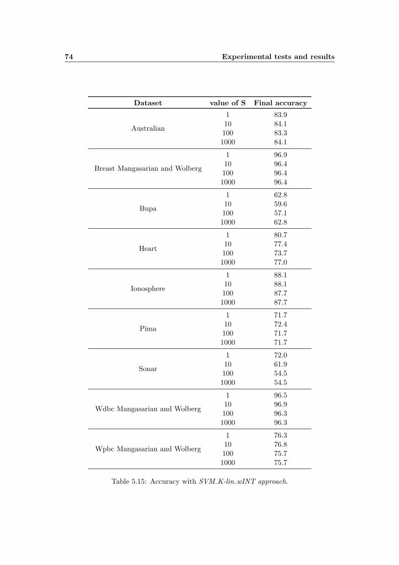
74 Experimental tests and results
Dataset value of S Final accuracy
Australian
1 83.910 84.1100 83.31000 84.1
Breast Mangasarian and Wolberg
1 96.910 96.4100 96.41000 96.4
Bupa
1 62.810 59.6100 57.11000 62.8
Heart
1 80.710 77.4100 73.71000 77.0
Ionosphere
1 88.110 88.1100 87.71000 87.7
Pima
1 71.710 72.4100 71.71000 71.7
Sonar
1 72.010 61.9100 54.51000 54.5
Wdbc Mangasarian and Wolberg
1 96.510 96.9100 96.31000 96.3
Wpbc Mangasarian and Wolberg
1 76.310 76.8100 75.71000 75.7
Table 5.15: Accuracy with SVM K-lin wINT approach.

Chapter 6
Software
6.1 Used software
6.1.1 CPLEX
IBM ILOG CPLEX Optimization Studio (often informally referred to simply as
CPLEX) is an optimization software package.
The CPLEX Optimizer was named after the simplex method as implemented
in the C programming language, although today it provides additional methods for
mathematical programming and offers interfaces other than just C. It was originally
developed by Robert E. Bixby and was offered commercially starting in 1988 by
CPLEX Optimization Inc., which was acquired by ILOG in 1997; ILOG was subse-
quently acquired by IBM in January 2009. CPLEX continues to be actively developed
under IBM [3].
CPLEX represents one of the most efficient software application, among those we
can find nowadays, created to solve LP and mixed-integer problems.
Precisely, this software enables the user to:
� Solve linear programming problems, even with thousands of variables and con-
straints, through the simplex algorithm (using either primal or dual variants)
and the barrier method;
� Solve integer programming problems, through procedures based on implicit enu-
meration (i.e. branch and bound);
� Solve quadratic (mixed-integer) problems.
There are two possible ways to interact with CPLEX:
� Writing a linear (integer) programming model in a text file, in the so-called LP
format, directly by the user or through a proper software (i.e. GAMS, AMPL,
OPL), that is then passed to the solver;

76 Software
� Using the API of the solver, implementing an interface through source code.
We choose the first alternative, that allows for a better check and debug of the
misclassification.
6.1.1.1 Command line code
Since we use the interactive mode, we have to deal with some instructions that enable
us to run properly the solver software giving the CPLEX LP file as input (this file
format will be described in section 6.1.1.2).
First of all, from the command prompt on a UNIX/Linux system, we have to
move to the parent directory that contains the executable file of cplex. The run of
the program through the command
cplex
enables us to enter a CPLEX command prompt : the bash shell should change to
CPLEX>
We are now ready to submit the .lp file which contains the PL/PLI problem to be
optimized. In the following we will see the basic commands to obtain the optimized
solution we need (see [3] for all the other options about the use of the system).
With
read filemodel.lp
we let the system read the problem.
With
opt
we let the system start the branch-and-bound/branch-and-cut optimization of the
problem.
With
write filesolution.sol
we let the system write the solution file into the same directory where the program
is installed.
With
quit
we let CPLEX quit and return to the operating mode.
In figure 6.3, an example of interaction with CPLEX from the command shell is
given.

6.1 Used software 77
Some additional settings
During the optimization phase of CPLEX, some parameters or optimization options
can be set.
We will give all the relative details when talking about specific optimization runs
for the each specific problem.
6.1.1.2 lp file format
This file format is one of those accepted in input by CPLEX software.
CPLEX LP format is intended for coding LP/MIP problem data. It is a row-
oriented format that assumes the usual formulation of LP/MIP problem.
CPLEX LP file is a plain text file coded using the CPLEX LP format.
Figure 6.1: Example of CPLEX LP file.
The fundamental components of a CPLEX LP file are
Objective function definition (mandatory): it must appear at the be-
ginning of the file and must be introduced by the keyword
MINIMIZE
or
MAXIMIZE
followed by the function to be optimized;
Constraints section (mandatory): it is introduced by the keywords
SUBJECT TO
followed by a constraint in one or more rows, where the constant
term appears to the right;
Bounds section (optional, when not specified we intend every variable
to be nonnegative): it is introduced by the keyword
BOUNDS
followed by a bound specification for each variable on a new row;
Variables specification section (optional): it is introduced by the key-
word
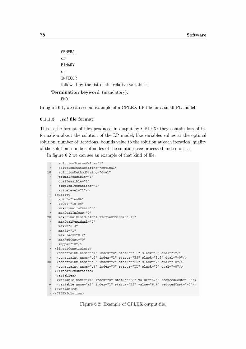
78 Software
GENERAL
or
BINARY
or
INTEGER
followed by the list of the relative variables;
Termination keyword (mandatory):
END.
In figure 6.1, we can see an example of a CPLEX LP file for a small PL model.
6.1.1.3 .sol file format
This is the format of files produced in output by CPLEX: they contain lots of in-
formation about the solution of the LP model, like variables values at the optimal
solution, number of iterations, bounds value to the solution at each iteration, quality
of the solution, number of nodes of the solution tree processed and so on . . .
In figure 6.2 we can see an example of that kind of file.
Figure 6.2: Example of CPLEX output file.

6.1 Used software 79
Figure 6.3: Example of use of CPLEX interactive optimizer.

80 Software
6.1.2 SVMlight
SVMlight is an implementation of Support Vector Machines in C code, developed by
Thorsten Joachims [5].
The main features we are interested in, for this thesis work, are the following:
� fast optimization algorithm
– working set selection based on steepest feasible descent
– caching of kernel evaluations
– use of folding in the linear case
� classification problems resolution
� support for standard kernel functions
SVMlight is an implementation of Vapnik’s Support Vector Machine for the problem
of pattern recognition, for the problem of regression, and for the problem of learning
a ranking function. The optimization algorithms used in SVMlight are described in
[Joachims, 2002a].
SVMlight consists of a learning module, called svm learn, and a classification mod-
ule, called svm classify. The classification module can be used to apply the learning
module to new examples.
For the running of the cited modules see section 6.1.2.1.
6.1.2.1 SVMlight installation and use
There are several ways of using SVMlight . They are all described in [20].
One of those possibilities is to download, in a UNIX/Linux environment, the
binary code for both the modules that compose SVMlight .
Opening a terminal shell and moving to the directory where we saved the binaries
and the input files, we just have to run first the learning module typing
svm learn [options] filetrain filemodel
For the whole list of available options see [5].
The options we used in our work are:
[-t] integer (kernel type selector – 0:default-linear, 1:polynomial, 2:Gaus-
sian)
[-g] float (value of gamma parameter for Gaussian kernel)
[-c] float (value of C parameter for quadratic optimization model)
[-a] string (file with λ values to be written)

6.1 Used software 81
The input file filetrain contains the training examples.
The result of svm learn is the model which is learned from the training data in
filetrain. The model is written to filemodel. To make predictions on test examples,
svm classify reads this file.
We can run the classification module typing
svm classify [options] filetest filemodel filesolution
For the whole list of available options see [5].
The test examples in filetest are given in the same format as the training ex-
amples.
For all test examples in filetest the predicted values are written to filesolution.
There is one line per test example in filesolution containing the value of the de-
cision function on that example. This value represents the signed sum computed by
the classifier
sign
[m∑i=1
yiλ∗iK(x,xi) + b∗
]
with the parameters values and the kernel values obtained though the run of svm learn
module.
The related class for each test item is the signed of the associate value stored in
filesolution.
In figure 6.4, an example of interaction with SVMlight from the command shell.
Figure 6.4: Example of use of the modules svm learn and svm classify of SVMlight .

82 Software
6.1.2.2 SVMlight file format
This file format is the one that is accepted in input by SVMlight software.
Each of the lines in input files represents one training example and is of the format
in figure 6.5:
Figure 6.5: Pattern line of SVMlight input files.
Where:
� target represents the class the item belongs to
� feature represents the ordered index number of the relative feature whose value
is given by
� value pairs (feature:value) where value = 0 can be skipped
Below in figure 6.6 we can see an example of such a line.
Figure 6.6: Example line of SVMlight input files.

6.1 Used software 83
6.1.3 LIBSVM
In this work we decided also to use another software, that can be directly downloaded
from the internet: LIBSVM.
Despite of the fact that we have already used SVMlight to realize classification, we
decided to have another comparison term, to test the correctness of our results.
We choose LIBSVM for its use simplicity, as we will see in the following.
LIBSVM is an integrated software for support vector classification, (C-SVC, nu-
SVC), regression (epsilon-SVR, nu-SVR) and distribution estimation (one-class SVM)
developed by Chih-Chung Chang and Chih-Jen Lin [23].
LIBSVM can be simply used through a Python script that makes everything
automatic, from data scaling to parameter selection.
LIBSVM provides a simple interface where users can easily link it with their own
programs. Some of the features of LIBSVM we are interested in include:
� Cross validation for model selection
� Probability estimates
� Various kernels (including precomputed kernel matrix)
6.1.3.1 LIBSVM installation and use
There are several ways of using LIBSVM. They are all described in [23].
One of those possibilities is to download, in a UNIX/Linux environment, the
Python script and the C++ source code that permits to realize classification.
To use this script, it is mandatory to install, always in a UNIX/Linux environment,
Python and gnuplot.
Opening a terminal shell and moving to the directory where we saved the Python
script, we just have to run it:
./easy filetrain [filetest]
For the whole list of available options see [23].
The options we used in our work are:
[-t] integer (kernel type selector – 0:default-linear, 1:polynomial, 2:gaus-
sian)
[-g] float (value of gamma parameter for gaussian kernel)
[-c] float (value of C parameter for quadratic optimization model)
[-a] string (file with λ values to be written)
The input file filetrain contains the training examples. The input file filetest
contains the test examples.

84 Software
Figure 6.7: Example of use of the LIBSVM Python script.
In figure 6.7, an example of interaction with LIBSVM from the command shell.
The outputs produced are the accuracies on the testset, in a file named filetrainoutput.txt,
.log files and a graphical interpretation of classification at the variation of the used
parameters (an example in figure 6.8).
Figure 6.8: Example of a graphical classification representation obtained with LIB-SVM.

6.1 Used software 85
6.1.3.2 LIBSVM file format
This file format is the one that is accepted in input by LIBSVM software.
This data format is exactly the same accepted in input by SVMlight software, so
see 6.1.2.2.
86 Software
6.1.4 R
The most-widely known and used software to perform Wilcoxon test is R.
R is a language and environment for statistical computing and graphics. It is a
GNU project which is similar to the S language and environment which was developed
at Bell Laboratories (formerly AT&T, now Lucent Technologies) by John Chambers
and colleagues.
R provides a wide variety of statistical (linear and nonlinear modelling, classical
statistical tests, time-series analysis, classification, clustering, . . . ) and graphical
techniques, and is highly extensible.
One of R’s strengths is the ease with which well-designed publication-quality plots
can be produced, including mathematical symbols and formulas where needed. Great
care has been taken over the defaults for the minor design choices in graphics, but
the user retains full control.
R is available as Free Software under the terms of the Free Software Founda-
tion’s GNU General Public License in source code form. It compiles and runs on a
wide variety of UNIX platforms and similar systems (including FreeBSD and Linux),
Windows and MacOS.
There are two possible ways of using R:
� as a programming language, that has its own libraries to be linked;
� in interactive way.
6.1.4.1 Command line code
Since we use the interactive alternative, we have to deal with some instructions that
enable us to run properly the software to realize the statistical computations we need.
The run of the program through the command
R
enables us to enter a R command prompt : the bash shell should change to
R>
We are now ready to type three simple commands that perform the Wilcoxon
test.
With
a = c(x1,x2,...,xn)
We submit the first array of percentage accuracies.
With

6.1 Used software 87
b = c(y1,y2,...,yn)
We submit the second array of percentage accuracies.
With
wilcox.test (a,b, paired=TRUE)
We let the system performs the test – defining that the null hypothesis is that the
methods compared are equal.
Since R provides also the commands for redirect input and output, we chose this
quick alternative.
The previously described commands are written, one for line, in a .txt file, for
example the accur for Wilcoxon.txt in figure 6.9.
Figure 6.9: Example of LIBSVM input file.
If we want the result of the performed test to be written in a file name, for example,
result Wilcoxon.txt, we just have to type:
R < accur for Wilcoxon.txt --no-save > result Wilcoxon.txt
Where --no-save is the default argument (that nevertheless must be declared) that
specifies not to save the R workspace at exit.
The output produced contains the lines in figure 6.10.
Figure 6.10: Significative output lines from R software for Wilcoxon test.

88 Software
6.2 Implemented software
In the following an overview about the software we needed to implement and execute
for our tests.
6.2.1 C source code
As we saw in section 6.1, we used software directly downloaded from the web.
The use of that software required the implementation of several programs, written
in C code, that enabled us to realize an adequate interface to the software itself.
In figure 6.11, we schematically take a vision of the whole procedure (that inte-
grates the use of implemented and downloaded software) which permits us to simulate
the overall operating process of the Support Vector Machines. And also, with some
proper changes, of other numerous variants, implemented in this thesis work, of the
classical problem.
The starting point of the whole procedure is represented by the dataset file,
that is the file containing the specific dataset directly downloaded from the UCI
Repository [21].
Dataset stored in the aforesaid repository have not got a predefined structure: in
general everyone has items and features saved in a different format.
Some have just numerical attributes, but however they can be stored in different
ways: an item for each line, with attributes separated by commas, or by hyphens,
or by tabs, or dots, and so on. Some other datasets have also categorical attributes:
they have to be converted in binary attributes as seen in 5.1. Other datasets contain
even literal attributes, that first of all have to be converted in categorical attributes
and then to numerical ones.
Parser 1
Parser 1 is an executable that “extracts” the dataset from its original format and
structures it in a particular format that is the same for all the datasets.
Between all the possible formats we chose the one that is accepted in input either
by SVMlight and by LIBSVM (see 6.1.2.2 for details). That way, we could also have
the possibility of making a debug of our code in the first phases of our experimentation
and also of comparing the final accuracies produced by our approaches with the ones
produced by these well known and reliable software.
Beside the formatting of the dataset, Parser 1, receiving in input a seed for the C
method srand(), produce also the random division of the dataset in the 710 training
and the 310 test set.

6.2 Implemented software 89
Figure 6.11: Scheme flow for our SVM implementation.

90 Software
Pseudocode 6.1: Pseudocode for the extraction of n train different indexes between 0 andn train-1.
1 init seed s2 init array of different indexes el[n_train]3 r = rand() % n_train4 t_e = 0 // number of taken elements5
6 whilewhilewhile (t_e < n_train)7 found = false8 forforfor (i from 0 to t_e -1)9 ififif (el[i] == r)
10 found = true11 breakbreakbreak12 ififif (found == false)13 el[t_e] = r14 t_e++15 r = rand() % n_train
Random indexes produced with the procedure in listing 6.1, are placed in ascend-
ing order. Then the lines with the corresponding number equal to each index are
extracted from the original dataset file and printed in a new file that represents the
training set, as described in listing 6.2.
Complementary indexes, at the same time, allow to extract the remaining dataset
items, which will form the test set.
Pseudocode 6.2: Pseudocode for the extraction of the training set from the dataset.
1 init training matrix t_m[n_train ][# feature]2 c_r = 0 // number of the currently read row of the dataset3 sc = 0 // index for scanning the array of random ordered indexes4 line = read() //read a line of the dataset5
6 whilewhilewhile (c_r < n_dataset)7 ififif (c_r = el[sc])8 forforfor (each feature k)9 t_m[c_r][k] = feature k of line #c_r
10 c_r++11 sc++12 elseelseelse13 c_r++14 line = read()
Parser 1, according to [22], realizes also the normalization of the dataset items,
subtracting the mean and dividing by the standard deviation, both calculated on the
training set items.
Pseudocode 6.3: Pseudocode for the calculation of mean and standard deviation and forthe normalization of the training set.
1 init array of mean values of the attributes mean[# features]2
3 forforfor (i from 0 to #features -1)

6.2 Implemented software 91
4 forforfor (j from 0 to #n_train -1)5 mean[i] = mean[i] + t_m[j][i]6 mean[i] = mean[i]/ n_train7
8 init array of standard deviations stdr_dev [# features]9
10 forforfor (i from 0 to #features -1)11 forforfor (j from 0 to #n_train -1)12 stdr_dev[i] = stdr_dev[i] + (t_m[j][i] - mean[i])ˆ213 stdr_dev[i] = sqrt(stdr_dev[i]/( n_train -1))14
15 forforfor (i from 0 to #features -1)16 forforfor (j from 0 to #n_train -1)17 t_m[i][j] = (t_m[i][j] - mean[i])/ stdr_dev[i]
In progress, during the experimentations, Parser 1 has been further complicated
in order to realize also the division of the training set in the 5 folds to be used during
5-fold cross validation (the procedure is similar to the one described in pseudocode
6.1 and 6.2).
ModelConstructor
ModelConstructor is the executable that constructs the mathematical model in .lp
file format, the one accepted in input by CPLEX (for details see 6.1.1.2).
Obviously lots of model constructors have been implemented because each differ-
ent mathematical model we tested is formatted by a different code.
The constructor, in order:
� Reads the training set;
� Constructs the relative kernel matrix (pseudocode in listing 6.4);
� Computes the coefficients of the objective function and the bounds;
� Formats the relative .lp model (pseudocode in listing 6.5).
Pseudocode 6.4: Pseudocode for the computation of the kernel matrix.
1 init kernel matrix k[n_train ][ n_train]2 init gamma // parameter of Gaussian kernel3
4 forforfor (i from 0 to n_train -1)5 forforfor (j from 0 to n_train -1)6 sum = 07 forforfor (k from 0 to #features -1)8 sum = sum + (t_m[j][k] - t[i][k])ˆ29 sum = - sum * gamma
10 k[i][j] = exp(sum)
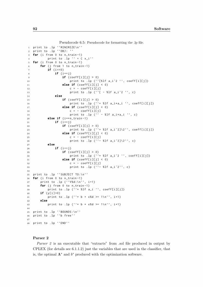
92 Software
Pseudocode 6.5: Pseudocode for formatting the .lp file.
1 print to .lp ’’MINIMIZE\n’’2 print to .lp ’’OBJ: ’’3 forforfor (i from 0 to n_train -1)4 print to .lp ’’ + C x_i’’5 forforfor (i from 0 to n_train -1)6 forforfor (j from 1 to n_train -1)7 ififif (i==0)8 ififif (i==j)9 ififif (coeff[i][j] > 0)
10 print to .lp (’’[%lf a_iˆ2 ’’, coeff[i][j])11 elseelseelse ififif (coeff[i][j] < 0)12 c = - coeff[i][j]13 print to .lp (’’[ - %lf a_iˆ2 ’’, c)14 elseelseelse15 ififif (coeff[i][j] > 0)16 print to .lp (’’+ %lf a_i*a_i ’’, coeff[i][j])17 elseelseelse ififif (coeff[i][j] < 0)18 c = - coeff[i][j]19 print to .lp (’’ - %lf a_i*a_i ’’, c)20 elseelseelse ififif (i==n_train -1)21 ififif (i==j)22 ififif (coeff[i][j] > 0)23 print to .lp (’’+ %lf a_i ˆ2]\2’’, coeff[i][j])24 elseelseelse ififif (coeff[i][j] < 0)25 c = - coeff[i][j]26 print to .lp (’’- %lf a_i ˆ2]\2’’, c)27 elseelseelse28 ififif (i==j)29 ififif (coeff[i][j] > 0)30 print to .lp (’’+ %lf a_iˆ2 ’’, coeff[i][j])31 elseelseelse ififif (coeff[i][j] < 0)32 c = - coeff[i][j]33 print to .lp (’’- %lf a_iˆ2’’, c)34
35 print to .lp ’’SUBJECT TO:\n’’36 forforfor (i from 0 to n_train -1)37 print to .lp (’’V%d:\n’’, i+1)38 forforfor (j from 0 to n_train -1)39 print to .lp (’’+ %lf a_i ’’, coeff[i][j])40 ififif (y[i]>0)41 print to .lp (’’+ b + x%d >= 1\n’’, i+1)42 elseelseelse43 print to .lp (’’+ b + x%d >= 1\n’’, i+1)44
45 print to .lp ’’BOUNDS :\n’’46 print to .lp ’’b free’’47
48 print to .lp ’’END’’
Parser 2
Parser 2 is an executable that “extracts” from .sol file produced in output by
CPLEX (for details see 6.1.1.2) just the variables that are used in the classifier, that
is, the optimal Λ∗ and b∗ produced with the optimization software.
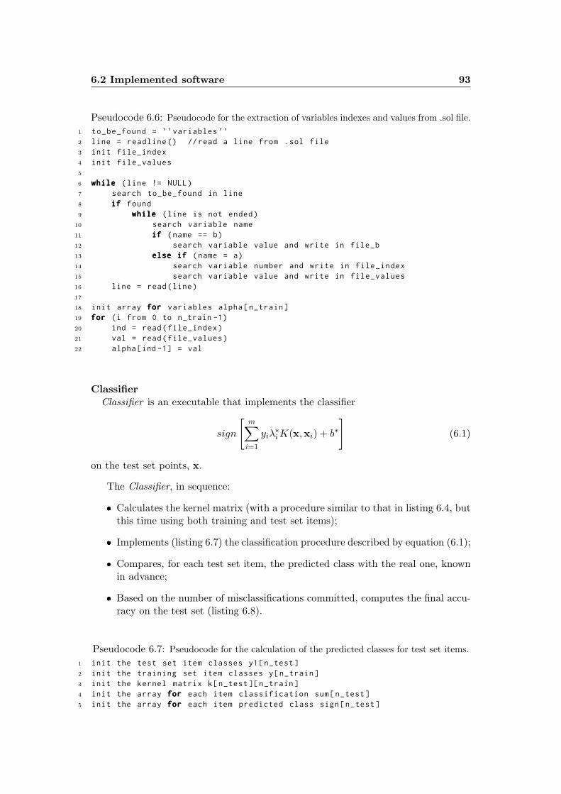
6.2 Implemented software 93
Pseudocode 6.6: Pseudocode for the extraction of variables indexes and values from .sol file.
1 to_be_found = ’’variables ’’2 line = readline () //read a line from .sol file3 init file_index4 init file_values5
6 whilewhilewhile (line != NULL)7 search to_be_found in line8 ififif found9 whilewhilewhile (line is not ended)
10 search variable name11 ififif (name == b)12 search variable value and write in file_b13 elseelseelse ififif (name = a)14 search variable number and write in file_index15 search variable value and write in file_values16 line = read(line)17
18 init array forforfor variables alpha[n_train]19 forforfor (i from 0 to n_train -1)20 ind = read(file_index)21 val = read(file_values)22 alpha[ind -1] = val
ClassifierClassifier is an executable that implements the classifier
sign
[m∑i=1
yiλ∗iK(x,xi) + b∗
](6.1)
on the test set points, x.
The Classifier, in sequence:
� Calculates the kernel matrix (with a procedure similar to that in listing 6.4, butthis time using both training and test set items);
� Implements (listing 6.7) the classification procedure described by equation (6.1);
� Compares, for each test set item, the predicted class with the real one, knownin advance;
� Based on the number of misclassifications committed, computes the final accu-racy on the test set (listing 6.8).
Pseudocode 6.7: Pseudocode for the calculation of the predicted classes for test set items.
1 init the test set item classes y1[n_test]2 init the training set item classes y[n_train]3 init the kernel matrix k[n_test ][ n_train]4 init the array forforfor each item classification sum[n_test]5 init the array forforfor each item predicted class sign[n_test]

94 Software
6
7 forforfor (i from 0 to n_test -1)8 sum[i] = 09 forforfor (j from 0 to n_train -1)
10 sum[i] = sum[i] + k[i][j]*alpha[j]*y[j]11 sum[i] = sum[i] + b12 ififif (sum > 0)13 sum[i] = 114 elseelseelse15 sum[i] = -1
Pseudocode 6.8: Pseudocode for the computation of the accuracy.
1 init the test set item classes y1[n_test]2 acc = 03
4 forforfor (i from 0 to n_test -1)5 ififif (y1[i] == sign[i])6 acc++7
8 final_accuracy = (acc/n_test )*100
6.2.2 Scripts
The tests performed in our experimentation require to repeat the whole procedure
several times.
As a matter of fact, we have to remember that every single accuracy obtained
in our experimentation is the mean value of three accuracies derived from a whole
procedure of 5-fold cross validation (5 iterations per parameters setting, the most of
the times we worked combining the simultaneous try of two parameters in a set of 5
values – that is, for each cross validation there are 25 executions, for a total of 125
sequential executions).
What we want to say is that it was necessary to implement proper scripts that
enable us to start just a single time the whole procedure and not to lose time compiling
and executing several times our codes.
Two examples of scripts, respectively for the realization of the SVM approach and
for the comparison between SVM approach and A1B0 approach on the dataset Heart
are given in Appendix D.
6.2.3 Hardware specifications
Tests have been performed on a machine Intel(R) Core(TM) i7-2670QM CPU @
2.20GHz, and 4GB RAM.

6.3 Instructions for compilation and execution of C source code 95
6.3 Instructions for compilation and execution of C sourcecode
First of all we will describe the structure of directories and subdirectories for saving,
compiling and executing all the source code implemented in this thesis project.
Secondly we will give some instructions for the use of the source code.
6.3.1 Directories structure
To compile and execute properly the source code implemented in our work, the fol-
lowing directories structure has to be created:
> CODES/
> File txt/
> Accuracy/
> Alpha/
> Dataset/
> PerSVMlight/
> SCRIPTS/
> 50 A1B0/
> 50 SVMlight/
> SVM aINT/
> SVM aAll TV/
> SVM K-gauss/
> SVM K-lin/
> SVM K-lin wINT/
> SVM Mixed/
> SVM MixedMu/
> SVM TV/
> SVM TV aINT/
> OUTPUT/
Where
� 50 A1B0/: refers to the realization of A1B0 approach;
� 50 SVMlight/: refers to the realization of SVM approach;

96 Software
� SVM aINT/: refers to the realization of classification using a INT model ;
� SVM aAll TV/: refers to the realization of classification using aAll TV model ;
� SVM K-gauss/: refers to the realization of classification using K-gauss model ;
� SVM K-lin/: refers to the realization of classification using K-lin model ;
� SVM K-lin wINT/: refers to the realization of classification using K-lin wINT
model ;
� SVM Mixed/: refers to the realization of classification using Mixed model ;
� SVM MixedMu/: refers to the realization of classification using MixedMu model ;
� SVM TV/: refers to the realization of classification using TV model ;
� SVM TV aINT/: refers to the realization of classification using TV a INT model ;
6.3.2 Where to save files
All the datasets, in the original format from UCI Repository, has to be saved in the
directory Dataset/ as
dataset <DATASET NAME>.txt
In the directory CODES/ have to be saved:
� C source codes: *.c files
� parameters for CPLEX: *.dat files
The directory containing the scripts, as we can see, is articulated in a set of
subdirectories, one for each of the mathematical models we tested.
There is a specific script, with proper parameters, for each dataset and for each
model to be tested1.
If the script subdirectory is, for example, SVM K-lin/, scripts named
throws<DATASET NAME> SVM K-lin.sh
have to be saved inside it.
If the subdirectory is SVM TV/, scripts named
throws<DATASET NAME> SVM TV.sh
have to be saved inside it.
And so forth for all the other scripts to be saved in all the other subdirectories of
directory SCRIPTS.
1A further work to be done could be to unify all the scripts for a model in a single script.
6.3 Instructions for compilation and execution of C source code 97
6.3.3 How to make the code work
Source code has been implemented and executed on a Linux environment, so correct-
ness and efficacy of the following instructions for the code execution is guaranteed
only for this type of platform.
6.3.3.1 Prerequisites
CPLEX
All the scripts, except the ones in directory 50 SVMlight/ and in directory 50 A1B0/,
requires the previous installation of the interactive CPLEX optimization solver (for
details see 6.1.1).
Notice that, reading a script, we can see that CPLEX is called typing
cplex
instead of
./cplex
That means that the execute permission for CPLEX has to be previously extended
to all.
This can be done typing, by the command prompt after moved to the directory
containing its executable
chmod a+x cplex
SVMlight
All the scripts in directory 50 SVMlight/ requires the previous installation of SVMlight
software (for details see 6.1.2).
Notice that, reading a script, we can see that module svm learn is called typing
svm learn
instead of
./svm learn
That means that the execute permission for svm learn has to be previously extended
to all.
This can be done typing, by the command prompt after have moved to the direc-
tory containing its executable
chmod a+x svm learn
The same considerations and consequent procedure above apply to module svm classify.
98 Software
6.3.3.2 Instructions for scripts runs
The organization of the source code has been thought with the aim of reducing the
number of programs to be used, trying to adopt a modular approach in the imple-
mentation of the code itself.
Conversely, the organization of the scripts is probably redundant, but permits to
have the total control over the specific codes execution.
In the following an example to clarify the use of the scripts.
First of all we have to make all the scripts executable. This can be done, from a
command prompt, moving to the directories where we can find the scripts and typing
chmod +x <SCRIPT NAME>
If we want to know the final mean accuracy for Ionosphere dataset, produced by
the classification approach based on the so-called TV model, we just have to move
with the command prompt to SCRIPTS/SVM TV/ directory and type
. ./throwsIONOSPHERE SVM TV validation.sh > outputfile.txt
This way, all the outputs produced by the optimization of CPLEX and eventually by
the execution of codes are redirected to an output file that can be use for controls
and debugs.
The final accuracy will be printed in a file named
Accuracy.txt
in directory OUTPUT/.

Conclusions and futureperspectives
This thesis work involved a particularly intense effort and dedication. It represented
for the student a challenge in the use and the acquisition of familiarity with new
software tools and new programming procedures.
We started our analysis from documentation about the theoretical foundations of
the functionality of Support Vector Machines. And we faced a practical experience
with SVM software tools like SVMlight and LIBSVM.
Afterwards, we first provided the global software implementation (comprehensive
of C programs, bash scripts and the use of CPLEX as interactive optimizer) that
allowed us to emulate a classic SVM, either with Gaussian or linear kernel. Starting
from its use we could perform a detailed investigation (that required several tests) of
the behaviour of its variables, which are determined by the resolution of an optimiza-
tion method and realize the final classification. That enabled us to confirm that the
behaviour of the system could suffer for the overfitting phenomenon. Knowing that,
we planned and implemented several alternative approaches, all aimed at ensuring a
functionality with less overfitting.
We observed, first of all, that the proposed approaches, which are alternative to
the classic SVM approach with Gaussian kernel, globally guarantee performances that
are equivalent, in terms of accuracy, to the ones produced by SVM approach itself.
Secondly, we understood that the performances of the overall functionality of a
SVM depends on three factors: the optimization model, the kernel type and the trial-
and-error validation of the parameters setting. In this context our analysis pointed
out that the Gaussian kernel tends to act like a good classifier by itself, characteristic
that considerably limits the rooms for improvement that we could think to achieve
acting on the remaining two factors.
Then we evaluated the entity of the superiority, in terms of accuracy, of the SVM
approach towards the one based just on the use of the final SVM classifier. In the
last one the variables values are fixed a priori in such a way to consider each point
in the system to give the same information for the classification of new items. This
evaluation allowed us to validate our thesis about the good nature of the Gaussian

100 Software
kernel as a classifier by itself: we observed an overall loss lower than the 6% of the
simplified approach towards the SVM one; besides, we noticed a bigger loss when
replicating the same comparison with the use of linear kernel.
Eventually, we terminated our analysis with the investigation of the behaviour of
linear kernel. The information collected during the previous experimentations tells us
that the use of this type of kernel surely permits more rooms for improvement. The
tests on linear kernel, aimed again to the reduction of overfitting, were performed at
the end of this thesis work. That was actually just a first attempt, that we could not
deepen for reasons of time.
At the end of our work some hints for future researches can be given: we think
that the same experimental tests conducted for Gaussian kernel, using alternative
mathematical models, can be replicated also for linear kernel with hopeful improve-
ments of the global performances. We suggest also to act with further modifications
on the simplified approach based on the use of the classifier without any kind of op-
timization and validation procedures: with the proper adaptations it could become a
valid alternative to the computationally expensive SVM approach, with comparable
accuracy but much less computational effort.

Appendix A
Detailed results for testsdescribed in section 5.2
In the following we report the detailed results obtained, for each dataset instance,
for the comparison of SVM approach towards A1B0 approach with Gaussian kernel.
The description of the tests is given in section 5.2.
For SVM approach, sparsity is defined as the number of zero component of the
vector Λ; its value is always 0% for A1B0.

102 Detailed results for tests described in section 5.2
AdultSeed SVM approach A1B0 approach SVM sparsity1 81.70 74.64 35.922 81.72 75.35 36.043 81.64 75.43 36.094 81.32 74.99 36.245 81.35 74.59 36.546 81.66 74.82 36.047 82.65 76.02 35.608 81.73 74.65 35.839 81.18 74.75 36.1610 81.28 75.69 35.5311 81.91 75.41 35.3912 81.22 74.72 36.0413 82.66 75.98 35.7014 82.24 75.38 35.8715 82.38 75.08 35.4816 81.61 74.90 36.0717 82.06 75.25 35.7318 81.91 75.25 36.2819 81.69 75.32 35.8120 82.23 75.72 35.5421 81.85 74.92 36.3822 81.69 75.08 36.2623 81.50 74.46 35.9524 81.87 75.04 36.3225 81.39 75.23 36.2526 81.94 75.20 36.1627 81.62 74.66 35.9728 80.99 74.35 36.6529 81.69 75.00 36.2830 81.47 74.71 36.3231 82.21 75.32 35.9232 81.98 74.89 35.6433 82.05 74.82 36.0034 81.98 74.89 35.5435 82.17 75.17 35.7436 81.86 75.86 36.0537 81.61 75.06 36.3538 82.56 75.41 35.6939 81.68 75.64 36.0240 81.65 75.36 36.0541 81.43 75.27 35.9542 81.64 74.67 35.9843 81.26 75.15 36.2344 81.55 74.83 36.2445 81.44 74.64 36.2446 82.23 75.30 36.1647 81.63 74.83 36.1948 82.07 75.15 35.6249 81.63 75.35 35.9350 82.54 75.40 35.79µ 81.79 75.11 35.99σ 0.39 0.38 0.28
Table A.1: Comparison table for dataset Adult.

103
AustralianSeed SVM approach A1B0 approach SVM sparsity1 77.78 76.33 16.772 83.09 85.99 17.393 83.57 79.71 16.774 78.26 81.64 16.155 82.61 85.02 17.186 83.57 84.54 17.607 79.71 82.61 16.368 85.51 84.54 14.299 85.51 81.64 16.9810 83.57 86.47 14.4911 78.26 84.06 15.9412 85.02 86.47 15.1113 81.16 85.99 12.2214 85.51 83.57 16.1515 82.61 84.06 13.0416 83.09 85.02 15.9417 82.13 83.57 15.1118 81.16 82.61 16.5619 85.02 85.99 15.7220 76.81 81.64 15.9421 84.06 85.02 15.3222 84.54 85.02 15.3223 80.68 80.19 16.7724 81.64 83.09 16.9825 81.64 83.09 15.9426 81.64 83.57 12.4227 78.74 82.13 13.8728 85.02 81.64 14.9129 85.02 84.06 16.1530 80.19 78.74 17.3931 79.71 82.13 15.9432 79.23 79.71 14.9133 82.13 82.61 16.5634 84.06 85.99 12.4235 85.99 85.51 15.5336 85.51 86.96 14.2937 87.44 88.41 15.1138 76.81 82.61 16.9839 84.54 85.02 13.0440 80.19 82.13 14.2941 85.99 87.44 16.7742 81.16 79.23 16.3643 82.13 83.57 12.6344 84.06 82.61 15.1145 85.51 86.47 16.1546 85.02 88.41 13.8747 84.54 83.09 16.1548 86.47 83.57 16.9849 85.51 84.54 15.7350 85.99 86.47 16.14µ 82.78 83.69 15.51σ 2.74 2.51 0.42
Table A.2: Comparison table for dataset Australian.

104 Detailed results for tests described in section 5.2
Breast Mangasarian and WolbergSeed SVM approach A1B0 approach SVM sparsity1 97.07 91.22 85.152 97.07 89.76 86.403 97.56 93.66 84.104 98.05 90.73 84.735 96.10 87.80 86.826 96.59 88.29 86.197 96.59 90.24 84.948 97.56 87.80 84.949 97.56 89.27 85.7810 98.05 92.68 82.4311 96.59 89.27 86.6112 95.61 86.34 86.4013 98.05 90.24 83.8914 97.56 89.76 84.1015 96.59 89.76 85.9816 96.59 85.37 85.7717 97.07 90.24 85.9818 99.02 93.17 82.2219 95.61 92.20 86.8220 97.56 93.66 84.7321 96.10 91.22 85.7722 96.59 91.71 85.9823 97.56 92.20 83.6824 97.07 88.29 85.3625 97.07 92.68 84.7326 97.07 89.76 85.9827 96.10 92.68 84.5228 96.59 87.80 85.7729 95.61 89.76 86.6130 95.61 87.32 85.9831 97.56 89.27 83.6832 97.56 90.24 84.9433 96.59 88.29 85.7734 97.56 89.76 85.3635 96.10 90.24 85.3636 94.63 90.24 85.1537 96.10 92.68 85.7738 98.05 89.27 83.8939 97.56 92.20 84.3140 95.61 89.27 87.0341 98.54 92.20 84.3142 96.59 94.15 85.7743 96.10 92.20 84.9444 97.07 86.83 85.3645 96.10 89.76 84.5246 97.07 90.24 85.1547 95.61 90.24 85.9848 96.10 90.24 84.1049 95.61 91.22 84.1050 98.05 90.24 83.89µ 96.84 90.27 85.15σ 0.91 1.97 1.08
Table A.3: Comparison table for dataset Breast Mangasarian and Wolberg.

105
BupaSeed SVM approach A1B0 approach SVM sparsity1 67.31 53.85 22.412 67.31 52.88 23.243 73.08 61.54 19.924 63.46 54.81 22.825 75.00 62.50 20.336 64.42 56.73 22.827 67.31 50.00 21.168 70.19 55.77 19.509 72.12 59.62 19.5010 73.08 54.81 18.6711 67.31 57.69 22.8212 74.04 59.62 16.1813 75.00 60.58 18.6714 66.35 59.62 22.4015 70.19 66.35 19.5016 72.12 58.65 18.6717 72.12 60.58 20.3318 69.23 53.85 18.2619 68.27 58.65 21.1620 71.15 63.46 21.1621 68.27 58.65 19.0922 74.04 61.54 19.9223 68.27 67.31 21.1624 72.12 61.54 22.8225 74.04 60.58 19.5026 72.12 61.54 17.0127 68.27 60.58 21.5828 72.12 56.73 20.7529 62.50 62.50 24.0730 67.31 58.65 22.4131 75.00 54.81 16.6032 73.08 51.92 19.0933 75.96 56.73 19.9234 76.92 58.65 19.5035 69.23 54.81 23.2436 59.62 48.08 25.3137 67.31 56.73 23.6538 71.15 58.65 21.1639 72.12 62.50 22.4140 68.27 62.50 22.8241 64.42 52.88 24.0742 76.92 59.62 16.6043 76.92 63.46 17.4344 67.31 54.81 22.4145 75.00 64.42 16.6046 71.15 56.73 20.3347 70.19 59.62 20.3348 73.08 61.54 19.9249 72.12 64.42 19.9250 72.12 62.50 16.60µ 70.52 58.73 20.51σ 3.90 4.11 2.25
Table A.4: Comparison table for dataset Bupa.
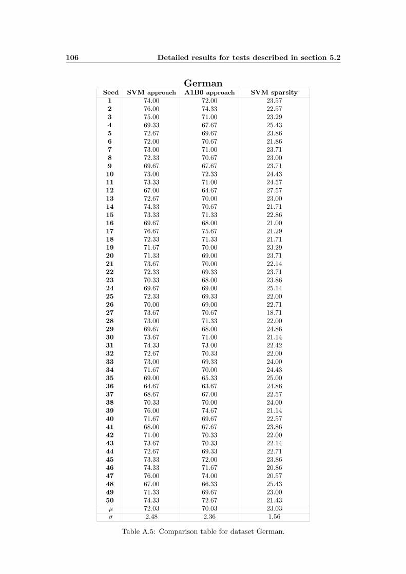
106 Detailed results for tests described in section 5.2
GermanSeed SVM approach A1B0 approach SVM sparsity1 74.00 72.00 23.572 76.00 74.33 22.573 75.00 71.00 23.294 69.33 67.67 25.435 72.67 69.67 23.866 72.00 70.67 21.867 73.00 71.00 23.718 72.33 70.67 23.009 69.67 67.67 23.7110 73.00 72.33 24.4311 73.33 71.00 24.5712 67.00 64.67 27.5713 72.67 70.00 23.0014 74.33 70.67 21.7115 73.33 71.33 22.8616 69.67 68.00 21.0017 76.67 75.67 21.2918 72.33 71.33 21.7119 71.67 70.00 23.2920 71.33 69.00 23.7121 73.67 70.00 22.1422 72.33 69.33 23.7123 70.33 68.00 23.8624 69.67 69.00 25.1425 72.33 69.33 22.0026 70.00 69.00 22.7127 73.67 70.67 18.7128 73.00 71.33 22.0029 69.67 68.00 24.8630 73.67 71.00 21.1431 74.33 73.00 22.4232 72.67 70.33 22.0033 73.00 69.33 24.0034 71.67 70.00 24.4335 69.00 65.33 25.0036 64.67 63.67 24.8637 68.67 67.00 22.5738 70.33 70.00 24.0039 76.00 74.67 21.1440 71.67 69.67 22.5741 68.00 67.67 23.8642 71.00 70.33 22.0043 73.67 70.33 22.1444 72.67 69.33 22.7145 73.33 72.00 23.8646 74.33 71.67 20.8647 76.00 74.00 20.5748 67.00 66.33 25.4349 71.33 69.67 23.0050 74.33 72.67 21.43µ 72.03 70.03 23.03σ 2.48 2.36 1.56
Table A.5: Comparison table for dataset German.

107
HeartSeed SVM approach A1B0 approach SVM sparsity1 76.54 81.48 20.112 79.01 80.25 21.163 72.84 76.54 22.224 85.19 87.65 19.055 79.01 83.95 20.636 79.01 82.72 20.117 79.01 81.48 18.528 81.48 80.25 18.529 75.31 79.01 20.6310 75.31 77.78 22.7511 77.78 88.89 19.0512 86.42 86.42 20.1113 82.72 82.72 22.7514 80.25 83.95 23.8115 75.31 76.54 20.6316 83.95 90.12 21.1617 79.01 85.19 20.6318 82.72 82.72 19.0519 80.25 76.54 21.1620 82.72 81.48 19.0521 77.78 77.78 22.2222 79.01 77.78 22.2223 79.01 80.25 23.8124 82.72 81.48 23.8125 85.19 86.42 17.9926 70.37 77.78 25.9327 80.25 87.65 18.5228 83.95 85.19 21.6929 77.78 80.25 20.6330 82.72 86.42 23.2831 76.54 76.54 25.9332 76.54 80.25 20.1133 76.54 74.07 23.2834 76.54 77.78 25.4035 76.54 79.01 21.6936 77.78 82.72 21.6937 82.72 81.48 22.7538 80.25 79.01 21.6939 81.48 85.19 22.7540 85.19 81.48 21.6941 83.95 86.42 20.1142 87.65 90.12 19.0543 79.01 81.48 21.1644 76.54 74.07 23.2845 77.78 81.48 21.6946 80.25 82.72 22.2247 86.42 88.89 16.9348 76.54 79.01 24.3449 81.48 80.25 23.8150 77.78 80.25 25.40µ 79.80 81.78 21.52σ 3.67 4.04 2.12
Table A.6: Comparison table for dataset Heart.

108 Detailed results for tests described in section 5.2
IonosphereSeed SVM approach A1B0 approach SVM sparsity1 92.45 80.19 38.782 91.51 69.81 40.413 96.23 67.92 40.824 94.34 71.70 42.455 93.40 73.58 41.636 90.57 65.09 44.497 96.23 79.25 37.558 97.17 80.19 40.419 96.23 73.58 39.1810 94.34 72.64 41.6311 94.34 77.36 40.8212 98.11 69.81 38.7813 95.28 65.09 42.4514 93.40 75.47 40.4115 92.45 66.98 44.9016 92.45 72.64 41.6317 92.45 67.92 46.1218 96.23 78.30 37.5519 96.23 74.53 42.6320 95.28 75.47 41.6321 93.40 76.42 42.4522 89.62 76.42 42.4523 89.62 74.53 41.6324 96.23 77.36 42.0425 95.28 72.64 38.3726 94.34 71.70 39.5927 92.45 80.19 40.8228 92.45 70.75 43.6729 94.34 75.47 41.2230 92.45 66.98 43.6731 94.34 74.53 42.0432 95.28 69.81 40.0033 94.34 78.30 41.6334 94.34 76.42 38.7835 93.40 71.70 40.8236 95.28 74.53 37.9637 96.23 72.64 42.0438 92.45 67.92 42.0439 92.45 80.19 39.5940 96.23 71.70 40.4141 95.28 71.70 41.6342 92.45 76.42 42.4543 90.57 78.30 37.9644 95.28 75.47 41.6345 98.11 73.58 38.3746 96.23 82.08 39.1847 90.57 68.87 44.9048 94.34 70.75 39.5949 90.57 61.32 42.0450 91.51 67.92 42.86µ 93.96 73.28 41.12σ 2.14 4.59 1.99
Table A.7: Comparison table for dataset Ionosphere.

109
PimaSeed SVM approach A1B0 approach SVM sparsity1 74.46 67.97 46.182 72.73 69.26 44.133 75.32 65.37 43.764 77.49 68.83 41.345 75.32 66.23 42.276 76.62 64.07 44.697 74.03 64.94 45.448 76.19 64.94 45.079 76.19 67.10 42.8310 73.59 61.90 44.5111 76.19 72.29 40.4112 80.09 68.40 40.4113 76.62 70.56 42.6414 78.35 64.94 42.2715 76.19 68.40 43.2016 74.03 60.61 43.0217 75.32 65.80 42.2718 71.43 56.28 48.6019 75.32 67.10 43.9520 73.16 66.67 40.9721 72.73 66.23 43.3922 76.19 67.53 43.2023 76.19 64.07 40.7824 78.35 68.83 40.2225 73.16 62.34 44.3226 78.35 65.80 42.4627 74.89 64.50 41.1528 74.89 59.31 45.4429 78.35 67.53 41.1530 76.62 64.50 42.4631 74.46 62.77 43.5832 75.32 67.97 42.8333 78.35 66.23 40.7834 78.35 70.13 40.4135 74.89 66.23 43.9536 78.79 71.86 40.2237 75.76 64.07 41.1538 77.92 64.50 43.7639 78.35 65.80 41.7140 79.22 64.50 40.6041 77.92 67.97 43.2042 74.46 65.37 42.8343 75.76 71.86 40.6044 74.89 63.20 44.3245 76.62 61.90 41.7146 77.49 65.80 42.2747 68.40 61.90 47.1148 76.62 64.94 41.9049 74.46 66.67 42.0950 73.59 65.37 43.58µ 75.80 65.83 42.82σ 2.20 3.13 1.86
Table A.8: Comparison table for dataset Pima.
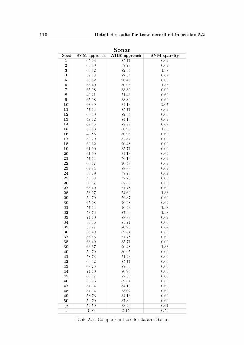
110 Detailed results for tests described in section 5.2
SonarSeed SVM approach A1B0 approach SVM sparsity1 65.08 85.71 0.692 63.49 77.78 0.693 60.32 82.54 1.384 58.73 82.54 0.695 60.32 90.48 0.006 63.49 80.95 1.387 65.08 88.89 0.008 49.21 71.43 0.699 65.08 88.89 0.6910 63.49 84.13 2.0711 57.14 85.71 0.6912 63.49 82.54 0.0013 47.62 84.13 0.6914 68.25 88.89 0.6915 52.38 80.95 1.3816 42.86 80.95 0.6917 50.79 82.54 0.0018 60.32 90.48 0.0019 61.90 85.71 0.0020 61.90 84.13 0.6921 57.14 76.19 0.6922 66.67 90.48 0.6923 69.84 88.89 0.6924 50.79 77.78 0.6925 46.03 77.78 0.0026 66.67 87.30 0.6927 63.49 77.78 0.6928 53.97 74.60 1.3829 50.79 79.37 0.6930 65.08 90.48 0.6931 57.14 90.48 1.3832 58.73 87.30 1.3833 74.60 88.89 0.6934 55.56 85.71 0.0035 53.97 80.95 0.6936 63.49 82.54 0.6937 55.56 77.78 0.6938 63.49 85.71 0.0039 66.67 90.48 1.3840 50.79 80.95 0.0041 58.73 71.43 0.0042 60.32 85.71 0.0043 68.25 87.30 0.0044 74.60 80.95 0.0045 66.67 87.30 0.0046 55.56 82.54 0.6947 57.14 84.13 0.6948 57.14 73.02 0.6949 58.73 84.13 0.6950 50.79 87.30 0.69µ 59.59 83.49 0.61σ 7.06 5.15 0.50
Table A.9: Comparison table for dataset Sonar.
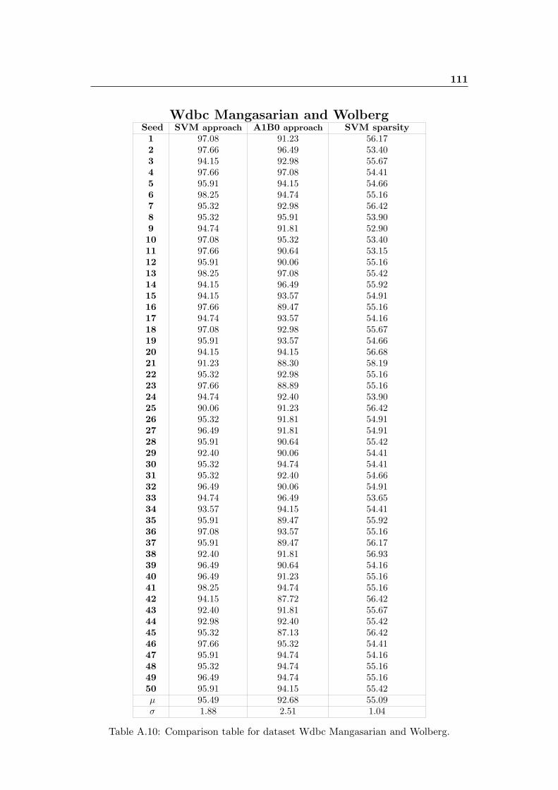
111
Wdbc Mangasarian and WolbergSeed SVM approach A1B0 approach SVM sparsity1 97.08 91.23 56.172 97.66 96.49 53.403 94.15 92.98 55.674 97.66 97.08 54.415 95.91 94.15 54.666 98.25 94.74 55.167 95.32 92.98 56.428 95.32 95.91 53.909 94.74 91.81 52.9010 97.08 95.32 53.4011 97.66 90.64 53.1512 95.91 90.06 55.1613 98.25 97.08 55.4214 94.15 96.49 55.9215 94.15 93.57 54.9116 97.66 89.47 55.1617 94.74 93.57 54.1618 97.08 92.98 55.6719 95.91 93.57 54.6620 94.15 94.15 56.6821 91.23 88.30 58.1922 95.32 92.98 55.1623 97.66 88.89 55.1624 94.74 92.40 53.9025 90.06 91.23 56.4226 95.32 91.81 54.9127 96.49 91.81 54.9128 95.91 90.64 55.4229 92.40 90.06 54.4130 95.32 94.74 54.4131 95.32 92.40 54.6632 96.49 90.06 54.9133 94.74 96.49 53.6534 93.57 94.15 54.4135 95.91 89.47 55.9236 97.08 93.57 55.1637 95.91 89.47 56.1738 92.40 91.81 56.9339 96.49 90.64 54.1640 96.49 91.23 55.1641 98.25 94.74 55.1642 94.15 87.72 56.4243 92.40 91.81 55.6744 92.98 92.40 55.4245 95.32 87.13 56.4246 97.66 95.32 54.4147 95.91 94.74 54.1648 95.32 94.74 55.1649 96.49 94.74 55.1650 95.91 94.15 55.42µ 95.49 92.68 55.09σ 1.88 2.51 1.04
Table A.10: Comparison table for dataset Wdbc Mangasarian and Wolberg.
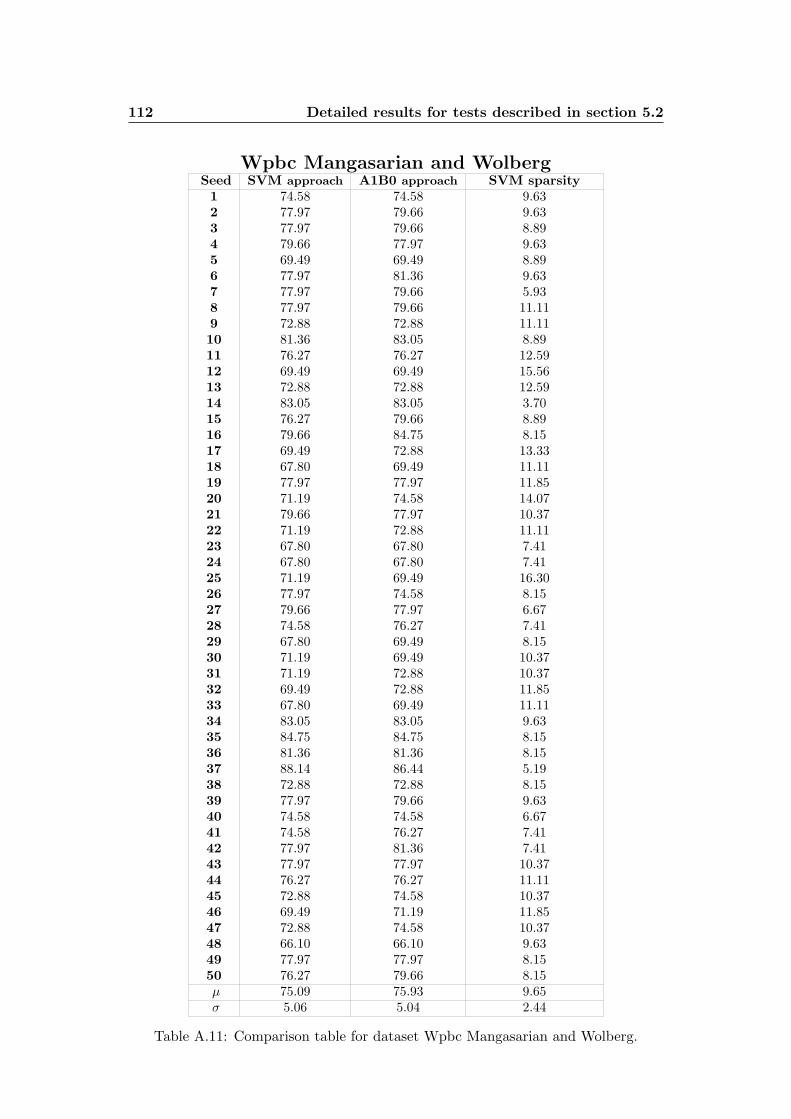
112 Detailed results for tests described in section 5.2
Wpbc Mangasarian and WolbergSeed SVM approach A1B0 approach SVM sparsity1 74.58 74.58 9.632 77.97 79.66 9.633 77.97 79.66 8.894 79.66 77.97 9.635 69.49 69.49 8.896 77.97 81.36 9.637 77.97 79.66 5.938 77.97 79.66 11.119 72.88 72.88 11.1110 81.36 83.05 8.8911 76.27 76.27 12.5912 69.49 69.49 15.5613 72.88 72.88 12.5914 83.05 83.05 3.7015 76.27 79.66 8.8916 79.66 84.75 8.1517 69.49 72.88 13.3318 67.80 69.49 11.1119 77.97 77.97 11.8520 71.19 74.58 14.0721 79.66 77.97 10.3722 71.19 72.88 11.1123 67.80 67.80 7.4124 67.80 67.80 7.4125 71.19 69.49 16.3026 77.97 74.58 8.1527 79.66 77.97 6.6728 74.58 76.27 7.4129 67.80 69.49 8.1530 71.19 69.49 10.3731 71.19 72.88 10.3732 69.49 72.88 11.8533 67.80 69.49 11.1134 83.05 83.05 9.6335 84.75 84.75 8.1536 81.36 81.36 8.1537 88.14 86.44 5.1938 72.88 72.88 8.1539 77.97 79.66 9.6340 74.58 74.58 6.6741 74.58 76.27 7.4142 77.97 81.36 7.4143 77.97 77.97 10.3744 76.27 76.27 11.1145 72.88 74.58 10.3746 69.49 71.19 11.8547 72.88 74.58 10.3748 66.10 66.10 9.6349 77.97 77.97 8.1550 76.27 79.66 8.15µ 75.09 75.93 9.65σ 5.06 5.04 2.44
Table A.11: Comparison table for dataset Wpbc Mangasarian and Wolberg.

Appendix B
A statistical tool: Wilcoxon Test
Wilcoxon Test is a nonparametric test used to compare two different series of measures
obtained on the same items. With that test we can compare two different instruments
or analytical procedure or operators.
There are tree different types of what is known in the scientific literature as
Wilcoxon test :
� Wilcoxon Two Sample Test;
� Wilcoxon Matched-Pairs Test;
� Wilcoxon Signed Rank Sum Test.
The test we will describe, that is the one we used, is the last one. Wilcoxon
Paired Signed Rank test is a nonparametric evaluation of paired differences. Pairs of
measurements forms the raw data, and the difference between the two members of
the pair is used to calculate the statistics. Wilcoxon is therefore the nonparametric
equivalent of the paired t test.
B.1 Prerequisites and hypothesis
Input data distribution. The test can be used on data that have a Gaussian dis-
tribution or on data that represent ordinal variables (recalling, from the theory,
that an ordinal variable is a variable whose value set V is a linearly ordered
set);
Measures on the same data. It is necessary that the items, on which the meth-
ods we are comparing are used, form exactly the same instances set for the
application of both the measurements;
Null hypothesis. We state that:
H0 : the first instances set is equal to the second one.

114 A statistical tool: Wilcoxon Test
That is: there is not a statistically significative difference between the use of
the first or the second method on the items.
Number of measurements. It is necessary to have more than a certain number of
measurements: usually between a few dozen and the Student threshold.
B.2 Procedure
To perform the test, the following steps have to be done:
� The test begins with the transformation of each couple of values (measure1 =
X1i, measure2 = X2i) into the absolute value of the difference between them:
|X1i −X2i| ∀i
� Couples that produces null differences do not give any kind of information in
the test, so they can be eliminated
if |X1i −X2i| then entryi isremoved
� The obtained differences are ordered for increasing absolute values. And then
a rank (unsigned quantity) is assigned to each of them, through a special pro-
cedure
|X1i −X2i| : Ri
� A sign is reassigned to each rank, depending on whether X1i−X2i was originally
positive or negative
ifX1i −X2i > 0 then R′i = Ri
ifX1i −X2i < 0 then R′i = −Ri
� The Wilcoxon test statistic value W is computed as the sum of the signed ranks
W =∑i
R′i
It can be demonstrated that, for samples with ndiff > 20, the test statistic W is
approximately normally distributed with mean µW and standard deviation σW .
The mean value of W is given by
µW =ndiff (ndiff + 1)
4
and its standard deviation by
σW =
√ndiff (ndiff + 1)(2ndiff + 1)
24

B.3 An example to describe the mathematical steps of the test 115
It is now possible to normalized the W distribution
Z =W − ndiff (ndiff+1)
4√ndiff (ndiff+1)(2ndiff+1)
24
Then, knowing the value of a certain occurrence of W , the relative value of Z can
be computed.
Recalling the concept of Rejection Region:
The rejection region is used in hypothesis testing. Let T be a test statis-
tic. Possible values of T can be divided into two regions: the acceptance
region and the rejection region. If the value of T comes out to be in the
acceptance region, the null hypothesis (the one being tested) is accepted,
or at any rate not rejected. If T falls in the rejection region, the null
hypothesis is rejected.
Thus, null hypothesis is rejected if the computed Z falls in the rejection region.
E.g., referring to the standard Gaussian distribution1 and assuming to accept a state-
ment with a statistical significativeness greater of equal to 95%, the decision rule states
that:
H0 is rejected if Z > 1.96 or Z < −1.96
otherwise H0 is accepted.
B.3 An example to describe the mathematical steps ofthe test
To make more clear the whole procedure, we extracted a small sample of measure-
ments we actually compared in our work. We have 20 couples of measurements of
accuracy calculated on as many dataset instances of Wpbc Mangasarian and Wolberg,
obtained randomly.
In table B.1 we have:
� Id or seed, it represents the identifier of the specific instance randomly defined
on the dataset;
� X1, it represents the first accuracy measurement, the one made with classic
SVM approach;
� X2, it represents the second accuracy measurement, the one made using just
the simple classifier, without solving mathematical models;
1In Appendix F the normal standard distribution table.

116 A statistical tool: Wilcoxon Test
id X1 X2 X1 −X2 |X1 −X2| rank signed rank1 74.58 74.58 0 0 - -
2 79.66 77.97 1.69 1.69 1/7 1/7
3 79.66 77.97 1.69 1.69 1/7 1/7
4 77.97 79.66 -1.69 1.69 1/7 -1/7
5 69.49 69.49 0 0 - -
6 81.36 77.97 3.39 3.39 1.25 1.25
7 79.66 77.97 1.69 1.69 1/7 1/7
8 79.66 77.97 1.69 1.69 1/7 1/7
9 72.88 72.88 0 0 - -
10 81.36 83.05 -1.69 1.69 1/7 -1/7
11 76.27 76.27 0 0 - -12 69.49 69.49 0 0 - -13 72.88 72.88 0 0 - -14 83.05 83.05 0 0 - -
15 79.66 76.27 3.39 3.39 1.25 1.25
16 79.66 84.75 -5.09 5.09 3 -3
17 72.88 69.49 3.39 3.39 1.25 1.25
18 67.80 69.49 -1.69 1.69 1/7 -1/7
19 77.97 77.97 0 0 - -
20 71.19 74.58 -3.39 3.39 1.25 -1.25
Table B.1: Wilcoxon test table for a small sample on Wpbc Mangasarian and Wolbergdataset.
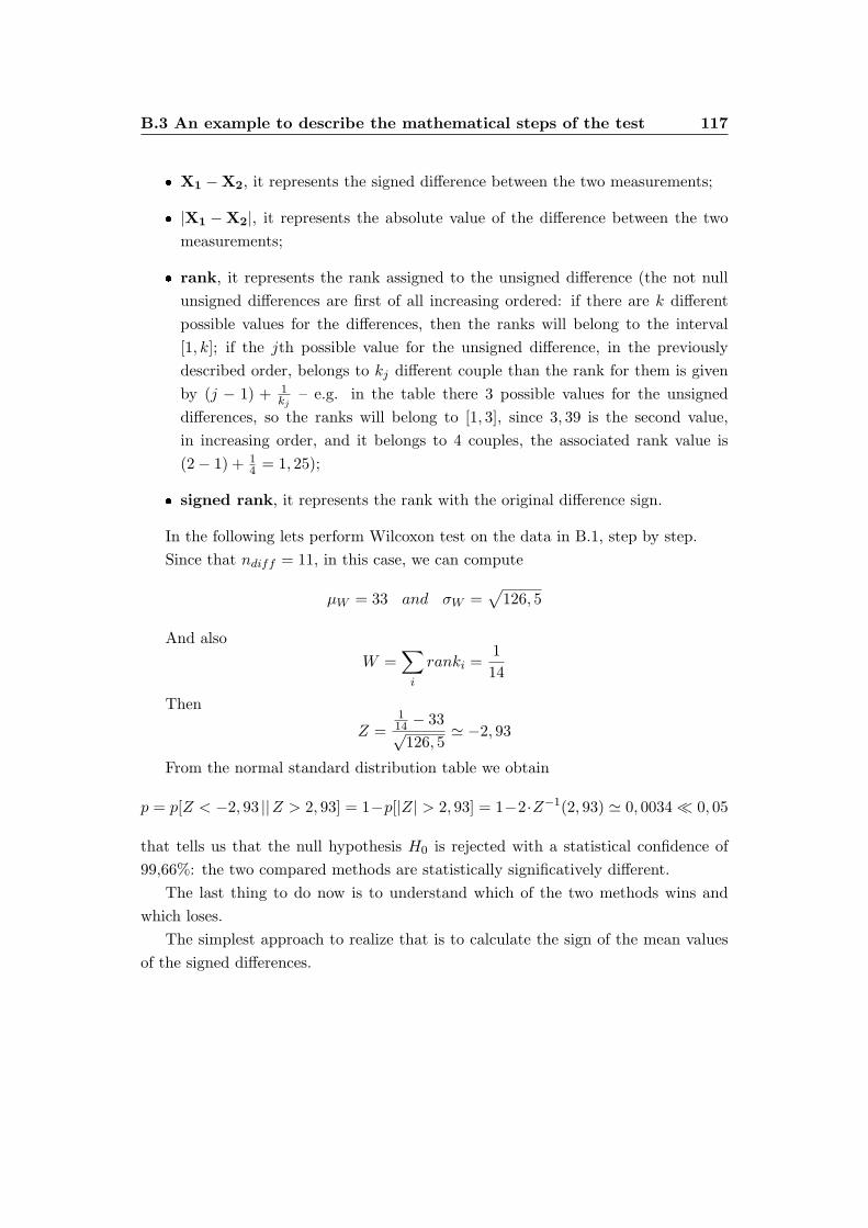
B.3 An example to describe the mathematical steps of the test 117
� X1 −X2, it represents the signed difference between the two measurements;
� |X1 −X2|, it represents the absolute value of the difference between the two
measurements;
� rank, it represents the rank assigned to the unsigned difference (the not null
unsigned differences are first of all increasing ordered: if there are k different
possible values for the differences, then the ranks will belong to the interval
[1, k]; if the jth possible value for the unsigned difference, in the previously
described order, belongs to kj different couple than the rank for them is given
by (j − 1) + 1kj
– e.g. in the table there 3 possible values for the unsigned
differences, so the ranks will belong to [1, 3], since 3, 39 is the second value,
in increasing order, and it belongs to 4 couples, the associated rank value is
(2− 1) + 14 = 1, 25);
� signed rank, it represents the rank with the original difference sign.
In the following lets perform Wilcoxon test on the data in B.1, step by step.
Since that ndiff = 11, in this case, we can compute
µW = 33 and σW =√
126, 5
And also
W =∑i
ranki =1
14
Then
Z =114 − 33√126, 5
≃ −2, 93
From the normal standard distribution table we obtain
p = p[Z < −2, 93 ||Z > 2, 93] = 1−p[|Z| > 2, 93] = 1−2·Z−1(2, 93) ≃ 0, 0034 ≪ 0, 05
that tells us that the null hypothesis H0 is rejected with a statistical confidence of
99,66%: the two compared methods are statistically significatively different.
The last thing to do now is to understand which of the two methods wins and
which loses.
The simplest approach to realize that is to calculate the sign of the mean values
of the signed differences.

118 A statistical tool: Wilcoxon Test

Appendix C
More detailed results
In the following we report some detailed results obtained during our several experi-
mental tests.
In table C.1 we can find the detailed accuracies obtained for each couple of pa-
rameters (C, γ), with the classic SVM approach, equipped with Gaussian kernel. The
values have been obtained without performing any kind of cross validation, just solv-
ing the classic quadratic model for the training procedure on the training set and
classifying, with the computed parameters, the test set items. As previously noticed,
the value of parameter γ that generally gives the best accuracies on our normalized
is γ = 0.1.
In table C.2 we can find the accuracies obtained at the variation of parameter C,
with the classic SVM approach, equipped with linear kernel. The values have been
obtained without performing any kind of cross validation, just solving the classic
quadratic model for the training procedure on the training set and classifying, with
the computed parameters, the test set items.
In table C.3 we report the detailed results obtained, for each dataset, for the
first evaluation of the use of a MIP model in SVM approach with linear kernel. The
description and the purposes of these last tests are given in section 4.2.2.
AustralianPPPPPPPPPC
γγγ0.1 1 10 100 1000
0.01 54.59 54.59 54.59 54.59 54.59
0.1 54.59 54.59 54.59 54.59 54.59
1 84.06 57.00 54.11 54.59 54.59
10 81.64 56.52 54.59 54.11 54.59
100 76.81 57.00 54.59 54.11 54.59

120 More detailed results
Breast Mangasarian and WolbergPPPPPPPPPC
γγγ0.1 1 10 100 1000
0.01 95.61 62.44 62.44 62.44 62.44
0.1 96.10 93.17 62.44 62.44 62.44
1 97.07 95.61 84.39 71.71 71.71
10 95.61 97.07 86.83 71.71 71.71
100 94.63 97.07 86.83 71.71 71.71
BupaPPPPPPPPPC
γγγ0.1 1 10 100 1000
0.01 52.88 52.88 52.88 52.88 52.88
0.1 52.88 52.88 52.88 52.88 52.88
1 64.42 65.38 53.85 53.85 53.85
10 64.42 65.38 56.73 53.85 53.85
100 62.50 62.54 56.73 53.85 53.85
HeartPPPPPPPPPC
γγγ0.1 1 10 100 1000
0.01 62.96 62.96 62.96 62.96 62.96
0.1 76.54 62.96 62.96 62.96 62.96
1 79.01 64.20 62.96 62.96 62.96
10 75.31 64.20 62.96 62.96 62.96
100 75.31 64.20 62.96 62.96 62.96
IonospherePPPPPPPPPC
γγγ0.1 1 10 100 1000
0.01 63.21 63.21 63.21 63.21 63.21
0.1 65.09 63.21 63.21 63.21 63.21
1 93.40 66.04 63.21 63.21 63.21
10 92.45 66.04 63.21 63.21 63.21
100 90.57 66.04 63.21 63.21 63.21
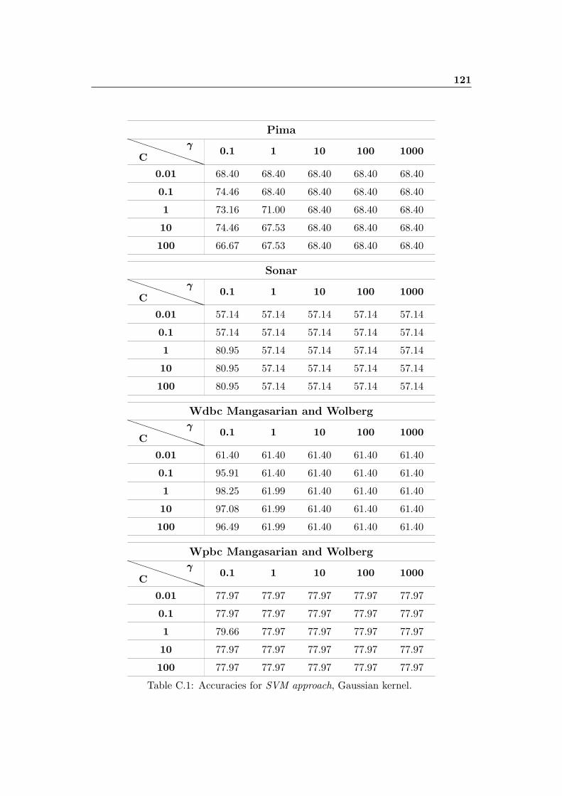
121
PimaPPPPPPPPPC
γγγ0.1 1 10 100 1000
0.01 68.40 68.40 68.40 68.40 68.40
0.1 74.46 68.40 68.40 68.40 68.40
1 73.16 71.00 68.40 68.40 68.40
10 74.46 67.53 68.40 68.40 68.40
100 66.67 67.53 68.40 68.40 68.40
SonarPPPPPPPPPC
γγγ0.1 1 10 100 1000
0.01 57.14 57.14 57.14 57.14 57.14
0.1 57.14 57.14 57.14 57.14 57.14
1 80.95 57.14 57.14 57.14 57.14
10 80.95 57.14 57.14 57.14 57.14
100 80.95 57.14 57.14 57.14 57.14
Wdbc Mangasarian and WolbergPPPPPPPPPC
γγγ0.1 1 10 100 1000
0.01 61.40 61.40 61.40 61.40 61.40
0.1 95.91 61.40 61.40 61.40 61.40
1 98.25 61.99 61.40 61.40 61.40
10 97.08 61.99 61.40 61.40 61.40
100 96.49 61.99 61.40 61.40 61.40
Wpbc Mangasarian and WolbergPPPPPPPPPC
γγγ0.1 1 10 100 1000
0.01 77.97 77.97 77.97 77.97 77.97
0.1 77.97 77.97 77.97 77.97 77.97
1 79.66 77.97 77.97 77.97 77.97
10 77.97 77.97 77.97 77.97 77.97
100 77.97 77.97 77.97 77.97 77.97
Table C.1: Accuracies for SVM approach, Gaussian kernel.

122 More detailed results
Australian
C 0.01 0.1 1 10 100
Accuracy 82.61 80.68 79.23 80.19 79.19
Breast Mangasarian and Wolberg
C 0.01 0.1 1 10 100
Accuracy 97.07 96.10 96.59 96.59 96.10
Bupa
C 0.01 0.1 1 10 100
Accuracy 53.85 59.62 66.35 66.35 66.35
Heart
C 0.01 0.1 1 10 100
Accuracy 80.25 80.25 81.48 79.01 81.48
Ionosphere
C 0.01 0.1 1 10 100
Accuracy 90.57 91.51 91.51 89.62 89.62
Pima
C 0.01 0.1 1 10 100
Accuracy 74.46 71.43 71.00 71.00 71.00
Sonar
C 0.01 0.1 1 10 100
Accuracy 84.13 80.95 76.19 76.19 76.19
Wdbc Mangasarian and Wolberg
C 0.01 0.1 1 10 100
Accuracy 95.32 97.08 97.08 95.91 95.91
Wpbc Mangasarian and Wolberg
C 0.01 0.1 1 10 100
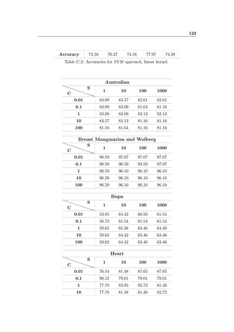
123
Accuracy 74.58 76.27 74.58 77.97 74.58
Table C.2: Accuracies for SVM approach, linear kernel.
AustralianPPPPPPPPPC
S1 10 100 1000
0.01 83.09 83.57 82.61 82.61
0.1 83.09 83.09 81.64 81.16
1 83.09 83.09 82.13 82.13
10 83.57 82.13 81.16 81.16
100 81.16 81.64 81.16 81.16
Breast Mangasarian and WolbergPPPPPPPPPC
S1 10 100 1000
0.01 96.59 97.07 97.07 97.07
0.1 96.59 96.59 93.59 97.07
1 96.59 96.10 96.10 96.10
10 96.59 96.10 96.10 96.10
100 96.59 96.10 96.10 96.10
BupaPPPPPPPPPC
S1 10 100 1000
0.01 53.85 64.42 60.58 61.54
0.1 56.73 61.54 61.54 61.54
1 59.62 65.38 63.46 64.46
10 59.62 64.42 63.46 63.46
100 59.62 64.42 63.46 63.46
HeartPPPPPPPPPC
S1 10 100 1000
0.01 76.54 81.48 87.65 87.65
0.1 90.12 79.01 79.01 79.01
1 77.78 83.95 92.72 81.48
10 77.78 81.48 81.48 82.72

124 More detailed results
100 77.78 81.48 81.48 81.48
IonospherePPPPPPPPPC
S1 10 100 1000
0.01 78.30 88.86 88.68 88.68
0.1 89.62 90.57 92.45 92.45
1 89.62 91.51 91.51 91.51
10 92.45 90.57 91.51 91.51
100 89.62 91.51 89.62 89.62
PimaPPPPPPPPPC
S1 10 100 1000
0.01 70.13 71.43 70.56 69.70
0.1 70.13 71.00 71.00 71.00
1 72.73 71.86 71.00 71.00
10 72.73 71.86 71.00 71.00
100 72.73 71.86 71.00 71.00
SonarPPPPPPPPPC
S1 10 100 1000
0.01 52.38 82.54 82.54 82.54
0.1 74.60 80.95 82.54 82.54
1 77.78 74.60 76.19 76.19
10 79.37 74.60 74.60 74.60
100 77.78 76.19 74.60 74.60
Wdbc Mangasarian and WolbergPPPPPPPPPC
S1 10 100 1000
0.01 94.15 96.49 97.08 97.08
0.1 97.08 97.66 97.08 97.08
1 96.49 97.08 97.08 97.08
10 97.66 96.49 96.49 96.49
100 95.32 95.91 95.91 95.91
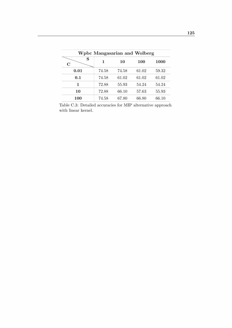
125
Wpbc Mangasarian and WolbergPPPPPPPPPC
S1 10 100 1000
0.01 74.58 74.58 61.02 59.32
0.1 74.58 61.02 61.02 61.02
1 72.88 55.93 54.24 54.24
10 72.88 66.10 57.63 55.93
100 74.58 67.80 66.80 66.10
Table C.3: Detailed accuracies for MIP alternative approachwith linear kernel.

126 More detailed results

Appendix D
Scripts
D.1 Example 1
In this section we report an example of a script for the simulation of the SVM approachon dataset Heart.
Script D.1: Script for SVM approach with 5-fold cross validation.
1 #!/bin/bash2 cdcdcd ..3 cdcdcd ..4 cdcdcd CODICI/5 gamma =(0.1 1 10 100 1000)6 C=(0.01 0.1 1 10 100)7 filedimensione=’’n_feature.txt ’’8 n_item =2709 forforfor (( r=1; r<=3; r++ ))
10 dododo11 file3accuracy=’’accuracy_finale_ ’’$r$ ’’.txt ’’12 gcc Parser1_HEART.c -o Parser1_HEART -lm13 ./ Parser1_HEART $r14 filetrainingFIN=’’File_txt/PerSVMlight/input_TrS_SVM_HEART_norm.txt
’’15 filetestFIN=’’File_txt/PerSVMlight/input_TeS_SVM_HEART_norm.txt ’’16 forforfor (( l=1; l<=5; l++ ))17 dododo18 forforfor (( j=0; j <=${#gamma [*]} -1; j++ ))19 dododo20 forforfor (( k=0; k <=${#C[*]} -1; k++ ))21 dododo22 fileaccuracy=’’File_txt/Accuracy/accuracy ’’${
gamma[j]}$’’_’’${C[k]}$’’_’’$l$ ’’.txt ’’23 filetraining=’’File_txt/PerSVMlight/
tutti_meno_ ’’$l$ ’’.txt ’’24 filetest=’’File_txt/PerSVMlight/’’$l$ ’’.txt ’’25 filenumelementi=’’File_txt/PerSVMlight/
num_elementi ’’$l$ ’’.txt ’’26 echoechoecho ’’esecuzione gamma ’’ ’’${gamma[j]}, ’’ ’’
C’’ ’’${C[k]}’’27 gcc ModelConstructor_SVM.c -o
ModelConstructor_SVM -lm

128 Scripts
28 ./ ModelConstructor_SVM ${gamma[j]} ${C[k]}$filetraining $filenumelementi$filedimensione
29 cplex < inputcpx.dat30 gcc Parser2.c -o Parser2 -lm31 ./ Parser2 $filenumelementi $filedimensione
$filetraining $filetest ${gamma[j]}$fileaccuracy
32 cdcdcd File_txt/33 DAESCLUDERE=dataset_HEART.txt34
35 forforfor i in $( ls );36 dododo37 ififif [[ $i == *.txt ]]38 thenthenthen39 ififif [[ $i != $DAESCLUDERE ]]40 thenthenthen41 rm $i42 fififi43 fififi44 ififif [[ $i == *.lp ]]45 thenthenthen46 rm $i47 fififi48 ififif [[ $i == *.sol ]]49 thenthenthen50 rm $i51 fififi52 donedonedone53
54 cdcdcd ..55 rm ModelConstructor_SVM56 rm Parser257
58 donedonedone59 donedonedone60 donedonedone61 gcc MaxCouple.c -o MaxCouple -lm62 ./ MaxCouple63 gcc ModelConstructorFIN_SVM.c -o ModelConstructorFIN_SVM -lm64 ./ ModelConstructorFIN_SVM $filetrainingFIN $filedimensione $n_item65 cplex < inputcpx.dat66 gcc Parser2FIN.c -o Parser2FIN -lm67 ./ Parser2FIN $filedimensione $filetrainingFIN $filetestFIN
$file3accuracy $n_item68
69 cdcdcd File_txt/70 DAESCLUDERE=dataset_HEART.txt71 forforfor i in $( ls );72 dododo73 ififif [[ $i == *.txt ]]74 thenthenthen75 ififif [[ $i != $DAESCLUDERE ]]76 thenthenthen77 rm $i78 fififi79 fififi

D.1 Example 1 129
80 ififif [[ $i == *.lp ]]81 thenthenthen82 rm $i83 fififi84 ififif [[ $i == *.sol ]]85 thenthenthen86 rm $i87 fififi88 donedonedone89 cdcdcd PerSVMlight/90 forforfor i in $( ls );91 dododo92 ififif [[ $i == *.txt ]]93 thenthenthen94 rm $i95 fififi96 donedonedone97 cdcdcd ..98 cdcdcd Accuracy/99 forforfor i in $( ls );
100 dododo101 ififif [[ $i == *.txt ]]102 thenthenthen103 rm $i104 fififi105 donedonedone106 cdcdcd ..107 cdcdcd ..108
109 rm Parser1_HEART110 rm MaxCouple111 rm ModelConstructorFIN_SVM112 rm Parser2FIN113 donedonedone114
115 gcc MeanFinalAccuracy.c -o MeanFinalAccuracy -lm116 ./ MeanFinalAccuracy117
118 rm accuracy_finale_1.txt119 rm accuracy_finale_2.txt120 rm accuracy_finale_3.txt121 rm MeanFinalAccuracy122 rm param_max_acc.txt123 rm n_feature.txt124 rm *.log125
126 cdcdcd ..127 cdcdcd X_SCRIPT
We can see that the execution of the code involves 4 for cycles:
� forforfor (( r=1; r <=3; r++ ))
enables us to repeat the whole procedure of classification, including the 5-fold
cross validation, 3 times, to compute the final mean accuracy;

130 Scripts
� forforfor (( l=1; l <=5; l++ ))
enables us to realize 5-fold cross validation (lines 22-25 rename properly at each
iteration training and validation sets in order to change them correctly);
� forforfor (( j=0; j <=${#gamma [*]} -1; j++ ))
enables us to try all the values of γ, defined at line 5;
� forforfor (( k=0; k <=${#C[*]} -1; k++ ))
enables us to try all the values of C, defined at line 6.
Scripts for all the other mathematical models used in out tests in general differs
from this one for the model constructor called at lines 27-28 and 63-64.
At lines 29 and 65 we can see a call of the optimization solver CPLEX, with a
redirection of the input from the file inputcpx.dat.
An example of that file can be as the one in listing D.2 (actually, since it contains
MIP settings, this .dat refers to the resolution of a MIP model).
Listing D.2: File with CPLEX settings.
1 set mip int tol 02 set timelimit 12003 set mip pol time 9004 r ModelSVM_HEART.lp5 opt6 w Sol_ModelSVM_HEART.sol7 disp pro var a* > Alpha\a.txt8 quit
It contains some settings used for the optimizer and the instructions for read,
optimize and write in a .sol file the got solution.
Lines 35-52 and 71-105 permit to remove all the files produced during the com-
putation, including occupying space .log files or .txt files written for debugging but
also, and it is a fundamental action, to remove the .sol file just finished to use. This
is important because CPLEX asks the user if he/she wants to overwrite a solution
file, and the software considers “no” to be the default answer. Since in our iterations
we re-use the same input.dat file, we need to remove the previous .sol file in the
working directory.
D.2 Example 2
In this section an example of a script for the fifty executions of the SVM approach in
parallel with A1B0 approach on fifty different instances of dataset HEART, without
the validation procedure.

D.2 Example 2 131
Script D.3: Script for the determination of the accurariesby SVM approach and A1B0 approach.
1 #!/bin/bash2 cdcdcd ..3 cdcdcd ..4 cdcdcd CODICI5 n_item =2706 n_feature=’’n_feature.txt ’’7 forforfor (( r=1; r <=50; r++ ))8 dododo9 echoechoecho ’’seed ’’ $r
10 gcc Parser1_HEART.c -o Parser1_HEART -lm11 ./ Parser1_HEART $r12 filetrainingset=’’File_txt/PerSVMlight/input_TrS_SVM_HEART_norm.txt
’’13 filetestset=’’File_txt/PerSVMlight/input_TeS_SVM_HEART_norm.txt ’’14 gcc Parser2_A1B0.c -o Parser2_A1B0 -lm15 ./ Parser2_A1B0 $n_item $n_feature $filetrainingset $filetestset16 donedonedone17
18 cdcdcd File_txt19 forforfor i in $( ls );20 dododo21 ififif [[ $i == *.txt ]]22 thenthenthen23 rm $i24 fififi25 donedonedone26 cdcdcd PerSVMlight27 forforfor i in $( ls );28 dododo29 ififif [[ $i == *.txt ]]30 thenthenthen31 rm $i32 fififi33 donedonedone34 cdcdcd ..35 cdcdcd ..36 cdcdcd ..37 cdcdcd X_SCRIPT

132 Scripts

Appendix E
C Code
In the following we report a listing of C code. It enables us to format the .lp file
that contains the model to be sent in input to CPLEX optimizer.
E.1 Example of Model constructor
Code E.1: Code for formatting .lp model.
1 #include <stdlib.h>2 #include <stdio.h>3 #include <math.h>4
5 int main( int argc , char *argv []){6
7 int i, j, elemento1;8 double elemento;9 char car;
10
11 //number of da tase t e lements12 int n_elementi = atoi(argv [3]);13 int n_train = (n_elementi *7) /10;14
15 //number of a t t r i b u t e s ( a f t e r preprocess ing )16 int n_dimensione;17 FILE *file_dim = fopen(argv[2], ’’r’’);18 fscanf(file_dim , ’’%d’’, &elemento1);19 n_dimensione = elemento1;20 fclose(file_dim);21
22 // optimal couple (\gamma, C) from va l i d a t i on procedure23 FILE *file_param = fopen(’’param_max_acc.txt’’, ’’r’’);24 fscanf(file_param , ’’%lf’’, &elemento);25 double gamma = elemento;26 fscanf(file_param , ’’%lf’’, &elemento);27 double C = elemento;28 fclose(file_param);29
30 // t ra in ing s e t31 FILE *file_trainingset;32 file_trainingset = fopen(argv[1], ’’r’’);

134 C Code
33
34 /* reading and saving t ra in ing s e t items */35
36 double **x;37 x = (double**) malloc(n_train * sizeof (double) );38 for(i=0; i<n_train; i++)39 x[i] = (double*) malloc(n_dimensione * sizeof (double) );40
41 int *y;42 y = ( int *) malloc(n_train * sizeof ( int));43
44 for (i = 0; i < n_train; i++){45 fscanf(file_trainingset , ’’%d’’, &elemento1);46 y[i] = elemento1;47 for (j = 0; j < n_dimensione; j++){48 fscanf(file_trainingset , ’’%d’’, &elemento1);49 fscanf(file_trainingset , ’’%c’’, &car);50 fscanf(file_trainingset , ’’%lf’’, &elemento);51 x[i][j] = elemento;52 }53 }54
55 fclose(file_trainingset);56
57 /* computing kerne l matrix */58
59 double ** kernel;60 kernel = (double**) malloc(n_train * sizeof (double) );61 for(i=0; i<n_train; i++)62 kernel[i] = (double*) malloc(n_train * sizeof (double) );63
64 int indice , l;65
66 for(i = 0; i < n_train; i++){67 for (j = 0; j < n_train; j++){68 kernel[i][j] = 0;69 }70 }71
72 for (indice =0; indice < n_train; indice ++){73 for(j = 0; j < n_train; j++){74 double somma = 0;;75 for(i = 0; i < n_dimensione; i++){76 somma = somma + (x[indice ][i] - x[j][i])*(
x[indice ][i] - x[j][i]);77 }78 kernel[indice ][j] = - somma*gamma;79 kernel[indice ][j] = exp(kernel[indice ][j]);80 }81 }82
83 /* computing model c o e f f i c i e n t s */84
85 double ** coeff;86 coeff = (double**) malloc(n_train * sizeof (double) );87 for(i=0; i<n_train; i++)88 coeff[i] = (double*) malloc(n_train * sizeof (double) );
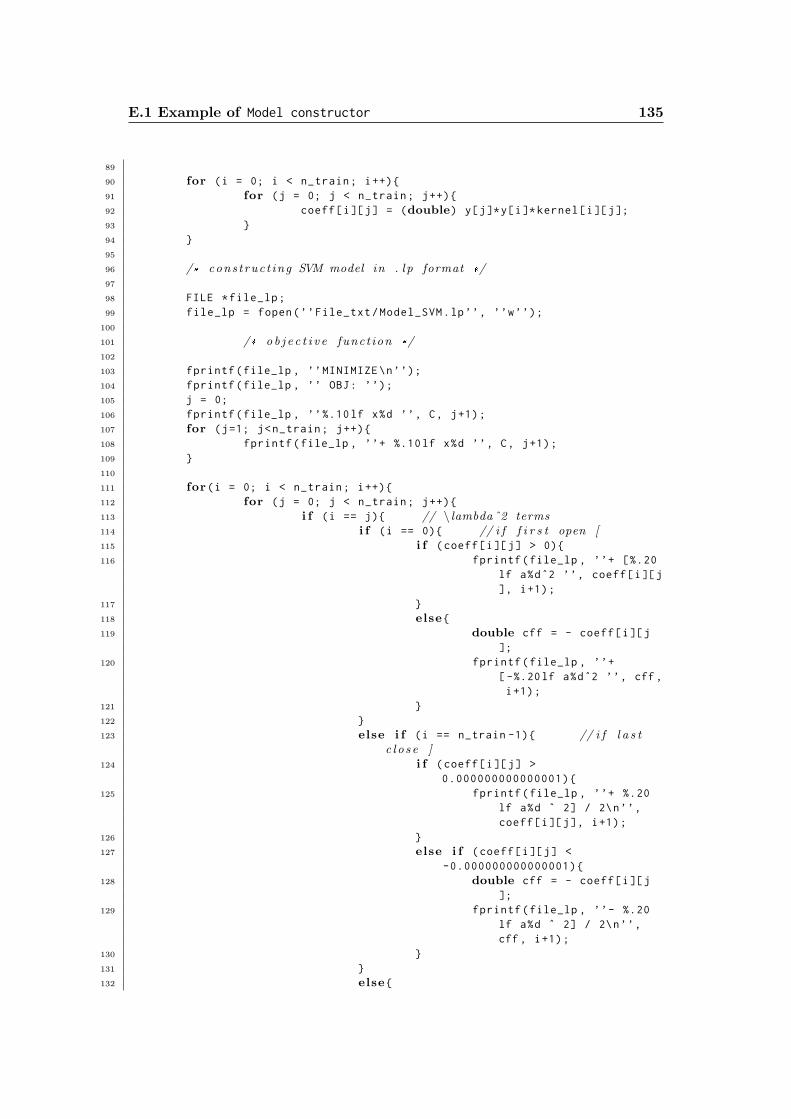
E.1 Example of Model constructor 135
89
90 for (i = 0; i < n_train; i++){91 for (j = 0; j < n_train; j++){92 coeff[i][j] = (double) y[j]*y[i]* kernel[i][j];93 }94 }95
96 /* cons t ruc t ing SVM model in . l p format */97
98 FILE *file_lp;99 file_lp = fopen(’’File_txt/Model_SVM.lp’’, ’’w’’);
100
101 /* o b j e c t i v e funct ion */102
103 fprintf(file_lp , ’’MINIMIZE\n’’);104 fprintf(file_lp , ’’ OBJ: ’’);105 j = 0;106 fprintf(file_lp , ’’%.10lf x%d ’’, C, j+1);107 for (j=1; j<n_train; j++){108 fprintf(file_lp , ’’+ %.10lf x%d ’’, C, j+1);109 }110
111 for(i = 0; i < n_train; i++){112 for (j = 0; j < n_train; j++){113 i f (i == j){ // \ lambdaˆ2 terms114 i f (i == 0){ // i f f i r s t open [115 i f (coeff[i][j] > 0){116 fprintf(file_lp , ’’+ [%.20
lf a%dˆ2 ’’, coeff[i][j], i+1);
117 }118 else {119 double cff = - coeff[i][j
];120 fprintf(file_lp , ’’+
[-%.20lf a%dˆ2 ’’, cff ,i+1);
121 }122 }123 else i f (i == n_train -1){ // i f l a s t
c l o s e ]124 i f (coeff[i][j] >
0.000000000000001){125 fprintf(file_lp , ’’+ %.20
lf a%d ˆ 2] / 2\n’’,coeff[i][j], i+1);
126 }127 else i f (coeff[i][j] <
-0.000000000000001){128 double cff = - coeff[i][j
];129 fprintf(file_lp , ’’- %.20
lf a%d ˆ 2] / 2\n’’,cff , i+1);
130 }131 }132 else {

136 C Code
133 i f (coeff[i][j] >0.000000000000001){
134 fprintf(file_lp , ’’+ %.20lf a%d ˆ 2 ’’, coeff[i][j], i+1);
135 }136 else i f (coeff[i][j] <
-0.000000000000001){137 double cff = - coeff[i][j
];138 fprintf(file_lp , ’’- %.20
lf a%d ˆ 2 ’’, cff , i+1);
139 }140 }141 }142 else { // \ lambda i *\ lambda j i<>j terms143 i f (coeff[i][j] > 0.000000000000001){144 fprintf(file_lp , ’’+ %.20lf a%d *
a%d ’’, coeff[i][j], i+1, j+1);145 }146 else i f (coeff[i][j] < -0.000000000000001)
{147 double cff = - coeff[i][j];148 fprintf(file_lp , ’’- %.20lf a%d *
a%d ’’, cff , i+1, j+1);149 }150 }151 }152 }153
154 /* bounds */155
156 fprintf(file_lp , ’’SUBJECT TO\n’’);157 for(i = 0; i < n_train; i++){158 int k = i+1;159 fprintf(file_lp , ’’ V%d: ’’, k);160 for (j = 0; j < n_train; j++){161 int h = j+1;162 i f (coeff[i][j] > 0.000000000000001){ //non
nega t i ve c o e f f i c i e n t163 i f (j == 0){ // i f f i r s t wi thout s ign164 fprintf(file_lp , ’’%.20lf a%d ’’,
coeff[i][j], h);165 }166 else { // i f not with s ign167 fprintf(file_lp , ’’+ %.20lf a%d ’’
, coeff[i][j], h);168 }169 }170 else i f (coeff[i][j] < -0.000000000000001){ //
nega t i ve c o e f f i c i e n t171 i f (j == 0){172 fprintf(file_lp , ’’%.20lf a%d ’’,
coeff[i][j], h);173 }174 else {

E.1 Example of Model constructor 137
175 double cff = coeff[i][j]*(-1);176 fprintf(file_lp , ’’- %.20lf a%d ’’
, cff , h);177 }178 }179 }180 i f (y[i] > 0)181 fprintf(file_lp , ’’+ b + x%d >= 1\n’’, i+1);182 else183 fprintf(file_lp , ’’- b + x%d >= 1\n’’, i+1);184 }185
186 /* v a r i a b l e s */187
188 fprintf(file_lp , ’’BOUNDS\n’’);189 for(i = 0; i < n_train; i++){190 int k = i+1;191 fprintf(file_lp , ’’ a%d >= 0\n’’, k);192 }193 fprintf(file_lp , ’’ - infinity <= b <= + infinity \n’’);194
195 for(i = 0; i < n_train; i++){196 int k = i+1;197 fprintf(file_lp , ’’ x%d >= 0\n’’, k);198 }199
200 /* c lo sure tag */201
202 fprintf(file_lp , ’’END\n’’);203
204 fclose(file_lp);205
206 return 0;207 }

138 C Code

Appendix F
Table of the normal distribution
z 0.00 0.01 0.02 0.03 0.04 0.05 0.06 0.07 0.08 0.090.0 .00000 .00399 .00792 .01197 .01595 .01994 .02392 .02790 .03188 .035860.1 .03983 .04380 .04776 .05172 .05567 .05962 .06356 .06749 .07142 .075350.2 .07926 .08317 .08706 .09095 .09483 .09871 .10257 .10642 .11026 .114090.3 .11791 .12172 .12552 .12930 .13307 .13683 .14058 .14431 .14803 .151730.4 .15542 .15910 .16276 .16640 .17003 .17364 .17724 .18082 .18439 .187930.5 .19146 .19497 .19847 .20194 .20540 .20884 .21226 .21566 .21904 .222400.6 .22575 .22907 .23237 .23565 .23891 .24215 .24537 .24857 .25175 .254900.7 .25804 .26115 .26424 .26730 .27035 .27337 .27637 .27935 .28230 .285240.8 .28814 .29103 .29389 .29673 .29955 .30234 .30511 .30785 .31057 .313270.9 .31594 .31859 .32121 .32381 .32639 .32794 .33147 .33398 .33646 .338911.0 .34134 .34375 .34614 .34849 .35083 .35314 .35543 .35769 .35993 .362141.1 .36433 .36650 .36864 .37076 .37286 .37493 .37698 .37900 .38100 .382981.2 .38493 .38686 .38877 .39065 .39251 .39435 .39617 .39796 .39973 .401471.3 .40320 .40490 .40658 .40824 .40988 .41149 .41309 .41466 .41621 .417741.4 .41924 .42073 .42220 .42364 .42507 .42647 .42786 .42922 .43056 .431891.5 .43319 .43448 .43574 .43699 .43822 .43943 .44062 .44179 .44295 .444081.6 .44520 .44630 .44738 .44845 .44950 .45053 .45154 .45254 .45352 .454491.7 .45543 .45637 .45728 .45818 .45907 .45994 .46080 .46164 .46246 .463271.8 .46407 .46485 .46562 .46637 .46712 .46784 .46856 .46926 .46995 .470621.9 .47128 .47193 .47257 .47320 .47381 .47441 .47500 .47558 .47615 .476702.0 .47725 .47778 .47831 .47882 .47932 .47982 .48030 .48077 .48124 .481692.1 .48214 .48257 .48300 .48341 .48382 .48422 .48461 .48500 .48537 .485742.2 .48610 .48645 .48679 .48713 .48745 .48778 .48809 .48840 .48870 .488992.3 .48928 .48956 .48983 .49010 .49036 .49061 .49086 .49111 .49134 .491582.4 .49180 .49202 .49224 .49245 .49266 .49286 .49305 .49324 .49343 .493612.5 .49379 .49396 .49413 .49430 .49446 .49461 .49477 .49492 .49506 .495202.6 .49534 .49547 .49560 .49573 .49585 .49598 .49609 .49621 .49632 .496432.7 .49653 .49664 .49674 .49683 .49693 .49702 .49711 .49720 .49728 .497362.8 .49745 .49752 .49760 .49767 .49774 .49781 .49788 .49795 .49801 .498072.9 .49813 .49819 .49825 .49831 .49836 .49841 .49846 .49851 .49856 .498613.0 .49865 .49869 .49874 .49878 .49882 .49886 .49889 .49893 .49897 .499003.1 .49903 .49906 .49910 .49913 .49916 .49918 .49921 .49924 .49926 .499293.2 .49931 .49934 .49936 .49938 .49940 .49942 .49944 .49946 .49948 .499503.3 .49952 .49953 .49955 .49957 .49958 .49960 .49961 .49962 .49964 .499653.4 .49966 .49968 .49969 .49970 .49971 .49972 .49973 .49974 .49975 .499763.5 .49977 .49978 .49978 .49979 .49980 .49981 .49981 .49982 .49983 .499833.6 .49984 .49985 .49985 .49986 .49986 .49987 .49987 .49988 .49988 .499893.7 .49989 .49990 .49990 .49990 .49991 .49991 .49991 .49992 .49992 .499923.8 .49993 .49993 .49993 .49994 .49994 .49994 .49994 .49995 .49995 .499953.9 .49995 .49995 .49995 .49996 .49996 .49996 .49996 .49996 .49997 .49997

140 Table of the normal distribution

Bibliography
[1] F. Poloni, Diversi approcci al problema della classificazione.Online documentation.http://fph.altervista.org/study/files/svm.pdf
[2] M. Sassi, A. Grissa, Clustering large data sets based on data compression techniqueand weighted quality measures.Proceedings of the 18th international conference on Fuzzy Systems, pagg 396-402,2009.
[3] IBM website.http://www-01.ibm.com/software/integration/optimization/cplex-optimizer/
[4] M. Stone Cross-validatory choice and assessment of statistical predictions.Journal of the Royal Statistical Society, B, 36(1), pagg 111-147, 1974.
[5] T. Joachims SVMlight Support Vector Machine.Online documentation.http://svmlight.joachims.org/
[6] G.C. Cawley, N.L.C. Talbot, Efficient leave-one-out cross-validation of kernelFisher discriminant classifiers.The journal of the Pattern Recognition Security, 36, pagg 2585-2592, 2003.
[7] T.S.Furey, N. Cristianini, N. Duffy, D.W. Bednarski, M. Schummer, D.Haussler,Support vector machine classification and validation of cancer tissue samples usingmicroarray expression data.Bioinformatics6(10), pagg 906-914, 2000.
[8] N. Stanevski, D. Tsvetkov, Using Support Vector Machine as a Binary Classifier.International Conference on Computer Systems and Technologies, pagg 1-14,2005.
[9] S. Tong, D. Koller, Support Vector Machine Active Learning with Applications toText ClassicationJournal of Machine Learning Research, pagg 45-66, 2001.
[10] N. Cristianini, J. Shawe-Taylor, An introduction to Support Vector Machines andother kernel-based learning methods.Cambridge University Press, 2000.

142 BIBLIOGRAPHY
[11] I. Guyon, J. Weston, S. Barnhill, Gene Selection for Cancer Classification usingSupport Vector MachinesMachine Learning, 46, pagg 389-422, 2002.
[12] D. Du, L. Qi, R.S. Womersley, Recent Advances in Nonsmooth OptimizationWorld Scientific, pag 99, 1995.
[13] B. Scholkopf, A.J. Smola, Learning with Kernels, Support Vector Machines, Reg-ularization, Optimization, and Beyond.Library of Congress Cataloging-in-Publication Data, 2002.
[14] E. Carrizosa, D. Romero Morales, Supervised classication and mathematical op-timization.Computers & Operations Research, pagg 1-16, 2012.
[15] C.J.C. Burges, A Tutorial on Support Vector Machines for Pattern Recognition.Data Mining and Knowledge Discovery, 2, pagg 121-167, 1998.
[16] R. Herbrich, J. Weston Adaptive Margin Support Vector Machines for Classifi-cation.In Proceedings of the Ninth International Conference on Articial Neural Networks,pagg 8805, 1999.
[17] A. Moschitti, R. Basili, VC-dimension.Academic material.http://www.uniroma2.it/didattica/WmIR/deposito/005_vc-dim.pdf
[18] E. Torrenti, Riconoscimento di facce in immagini generiche.Academic material.
[19] E. Ottaviani Tecniche di riconoscimento statistico. Academic material.
[20] SVMlight website.http://svmlight.joachims.org/
[21] UCI Learning Machine Repository website.http://archive.ics.uci.edu/ml/
[22] J.P. Brooks Support Vector Machines with the Ramp Loss and the Hard MarginLossOperation Research, pagg 1-13, 2011.
[23] LIBSVM website.http://www.csie.ntu.edu.tw/˜cjlin/libsvm/
[24] R website.http://www.r-project.org/
[25] A. Azzalini, B. Scarpa, Analisi dei dati e data mining.Springer, 2004.

BIBLIOGRAPHY 143
[26] D. Salvagnin, Cenni di Programmazione Lineare Intera.Academic material.
[27] L. Lamport, LaTeX, A Document Preparation System.Addison-Wesley Publishing Company, 1985.
[28] M. Goossens, S. Rahtz, F. Mittelbach, The LaTeX Graphics Companion.Addison-Wesley Publishing Company, 1997.
[29] Ubuntu website.http://www.ubuntu.com/
[30] Debianizzati website.http://guide.debianizzati.org/index.php/Guida_ai_comandi_da_terminale

144 BIBLIOGRAPHY

Acknowledgements
Inizio i miei sinceri ringraziamenti dal mio relatore, prof. Matteo Fischetti.
Estremamente disponibile e gentile, ha saputo sopportare le mie mille mail, senza
spazientirsi di fronte ai miei innumerevoli scoraggiamenti, ma, anzi, sapendomi sot-
tilmente e costantemente motivare.
Grazie per la fiducia ripostami, spero di non avere deluso le sue aspettative.
Grazie innanzitutto alla mia famiglia, che c’e sempre stata, c’e sempre e ci sara
sempre. Se sono vicina o se sono lontana. Se sono felice o se sono triste.
Grazie al mio papi preferito: sai coccolarmi senza viziarmi e, con un abbraccio e
poche parole, mi fai sentire capita e protetta come nessun altro.
Grazie alla mia mami : nonostante tutto mi sei sempre accanto ed esprimi per
me, con piu speranza di ogni altra persona, il desiderio piu importante: la mia felicita.
Grazie a mia sorella Anna : finalmente, crescendo, ti ho riscoperta e tu, spero,
hai riscoperto me. Ti voglio bene.
Grazie ai miei amici. Non mostro spesso quanto siate importanti per me, pertanto
voglio cogliere questa occasione per ricordarvelo.
Grazie ad Ale, per tutto quello (tanto) che abbiamo condiviso, dalle vacanze alle
gite all’orto botanico, dai weekend a casa tua post erasmus alle serate “in scatola” a
casa mia, dai miei costanti tentativi di distrarti a lezione alla tua pazienza nel farmi
compagnia in stazione a Mestre mentre attendevo la coincidenza. Sono felice che tu
ci sia nella mia vita.
Grazie ad Alvi, per la tua immensa pazienza e disponibilita, perche sei una delle
poche persone che ha accettato tante delle mie fragilita, per le quali provvedi a ras-
sicurarmi costantemente. Sei una gran persona, che si fa fatica a scoprire, ma per la
quale quella fatica vale proprio la pena. E “Ace” per un certo disegnino di pag 45 :)
Grazie ad Ari, per i tuoi consigli e la tua saggezza, ma soprattutto perche ogni
chiacchierata dopo tanto tempo e sempre ugualmente speciale.
Grazie a Bea, per le bilaterali confidenze.
Grazie a Bedo, perche sei il tipico amico che e presente nella vita di una persona

nelle dosi perfette, non troppo cozzo, non troppo distante, ti interessi a me ma non sei
invadente (a parte quando ti sogno durante gli incubi oppure quando vuoi infilarmi
un obiettivo in un occhio!).
Grazie a Daniele, per aver sopportato le mie mille domande su Ubuntu e i miei
innumerevoli sfoghi, e perche.... a sminuire sono bravi tutti! :P
Grazie a Davide, per credere in me.
Grazie a Dile, per essere la mia criminale preferita (che sa dirmi precisamente
che reato stiamo commettendo e qual e la relativa pena, in giorni ed euro) e per
essere sempre cosı felice di sentirmi e vedermi, come lo sono io di sentire e vedere te
d’altronde!
Grazie a Fede, perche mi vuoi bene senza dover necessariamente stare al centro del
palco, e perche sei saggia per due, sia per te che per me! Anche noi abbiamo condiviso
tanto, ci siamo fatte spalla a vicenda, abbiamo riso assieme e pianto assieme (tu un
bel po’ meno di me pero ;) ). Spero con il cuore che continueremo a spartire una
fettina di vita, perche adoro svegliarmi con un bradipo accanto la mattina.
Grazie a Fra, perche c’e sempre e vede sempre il buono in tutto; per i messaggi
che mi ricordano di non scordare che mi pensa sempre e mi augura in ogni momento
un sorriso.
Grazie a Giulia, per le sue chiamate “ma ciao!” tanto inaspettate quanto gradite.
Grazie a Giulio, perche al tuo posto non so come avrei fatto, e per fortuna tu ci
sei riuscito.
Grazie a Lorenzo, per aver accettato la sfida: mo’ so’ c***i tuoi!
Grazie a Lory, perche ai miei avvenimenti importanti tu non manchi mai, e non
immagini quanto sia bello per me che tu ci sia.
Grazie a Marco, perche ci provi SEMPRE e la cosa mi fa divertire da matti (a
te un po’ meno, I know).
Grazie a Marti, per i numerosi consigli che hai sfornato per me, assieme ad un
gregge di coccinelle! (ps: il Marco di prima non e il tuo)
Grazie a Miki, per la perseveranza nello starmi vicino. E per essere incapponita-
mente testardo come me.
Grazie a Nicole, perche sei a-d-o-r-a-b-i-l-e.
Grazie ad Oriez, per le belle montagne passate assieme, sperando di replicare.
Grazie a Ross, perche, anche se spesso tu ed io non siamo compatibili, sappiamo
comunque riconciliarci e volerci un gran bene a prescindere.
Grazie a Seba, perche nonostante tu sia burbero e lunatico, e io sia precisina
e paranoica, in fondo siamo una bella coppia di amici e sappiamo equilibratamente
capirci ed apprezzarci, sfotterci e mandarci a quel paese. Ridendo sempre un sacco :)
Grazie a Silvia, per essere un serbatoio di malizia.
Grazie a Teo, per chiamarmi con tutti quei nomignoli carini che mi sanno ringal-

luzzire l’autostima, per dedicare spesso il tuo tempo a rendermi partecipe della tua
vita quotidiana, facendomi sentire come una gradita e importante ospite del tuo spet-
tacolo, per volermi sempre sempre bene e non dimenticare mai di ricordarmelo.
Grazie poi a Dario, Andrea e Manu per le serate in scatola.
Grazie a Bob perche tieni molto a me.
Grazie a NM, per tutto il lavoro fatto in questi anni, anche se tanto temo le resti
da fare, perche non sa usare il computer -anche se ha un MAC- e perche si mette la
crema per le mani “da fighetta”.
Grazie a Paola, per aver mantenuto i rapporti dopo il liceo e perche ora posso
darti del tu.
Grazie ad Annalisa, perche e sempre bello vederti.
Grazie a Mat, per essere un cugino tanto introverso e timido quanto caro.
Varie ed eventuali....
Grazie a quell’essere peloso, scodinzolante, puzzolente, testardo e ronfante che
gira per la casa e mi fa compagnia mentre lavoro. Pronta per Camilla? ;)
Padova, 10 dicembre 2012.
Luci

.