European Journal of Operational Research 203 (2010) 673–683

Contents lists available at ScienceDirect

European Journal of Operational Research

journal homepage: www.elsevier .com/locate /e jor

Decision Support

A comprehensive analytical approach for policy analysis of system dynamics models

Mohamed Saleh a,1, Rogelio Oliva b,*, Christian Erik Kampmann c,2, Pål I. Davidsen d,3

a Decision Support Department, Faculty of Computers and Information, Cairo University, 5 Ahmed-Zwail Street, Orman–Giza, P.O. Box 12613, Egyptb Mays Business School, Texas A&M University, 301C Wehner – TAMU 4217, College Station, TX 77843, USAc Department of Innovation and Organizational Economics, Copenhagen Business School, Kilevej 14A-B, Room 3.82, DK-2000 Frederiksberg, Denmarkd System Dynamics Group, Department of Geography, University of Bergen, P.O. Box 7800, 5020 Bergen, Norway

a r t i c l e i n f o

Article history:Received 24 April 2008Accepted 15 September 2009Available online 20 September 2009

Keywords:System dynamicsLinear model analysisEigenvalue analysisLeverage points

0377-2217/$ - see front matter � 2009 Elsevier B.V. Adoi:10.1016/j.ejor.2009.09.016

* Corresponding author. Tel.: +1 979 862 3744; faxE-mail addresses: saleh@salehsite.info (M. Saleh),

1 Tel.: +20 2 33350 178; fax: +20 2 33350 109.2 Tel.: +45 4083 8444; fax: +45 3815 2540.3 Tel.: +47 55 58 41 34; fax +47 55 58 30 99.

a b s t r a c t

Formal tools to link system dynamics model’s structure to the system modes of behavior have recentlybecome available. In this paper, we aim to expand the use of these tools to perform the model’s policyanalysis in a more structured and formal way than the exhaustive exploratory approaches used to date.We consider how a policy intervention (a parameter change) affects a particular behavior mode by affect-ing the gains of particular feedback loops as well as how it affects the presence of that mode in the var-iable of interest. The paper demonstrates the utility of considering both of these aspects since the analysisprovides an assessment of the overall impact of a policy on a variable and explains why the impact occursin terms of structural changes in the model. Particularly in the context of larger models, this methodenables a much more efficient search for leverage policies, by ranking the influence of each model param-eter without the need for multiple simulation experiments.

� 2009 Elsevier B.V. All rights reserved.

1. Introduction

The purpose of a system dynamics (SD) intervention is to identify how structure and decision policies generate system behavior iden-tified as problematic, so that structural and policy oriented solutions can be identified and implemented (Forrester, 1961; Sterman, 2000).The approach relies on formal simulation models to capture the detailed complexity of the problem situation and to make reliable behav-ioral inferences. The field has devoted a great deal of attention to model validation and the kinds of explicit tests a model needs to pass (e.g.,Barlas, 1989; Barlas and Carpenter, 1990; Forrester and Senge, 1980; Oliva, 2003; Sterman, 2000). However, since SD modeling is problemdriven, the discipline also takes a functional perspective: validation is considered an iterative process of gradually building confidence inthe model as a ‘‘useful” representation of the problem at hand and the theoretical assumptions taken (van Horn, 1971). (See also Gass,1983; Miser, 1993; Mitroff, 1972; Roy, 1993; Smith, 1993, for evidence of this shift of validation in the OR/OM community).

Once confidence in the model has been attained, the generation of policy solutions is based on experimentation driven by the modelers’expertise (Forrester, 1961), or exhaustive what-if scenario analysis (Morecroft, 1988). These approaches rely on trial-and-error simulation,changing parameter values or switching individual links and feedback loops on and off, to discover important system elements and derivepolicy recommendations. The intuition guiding this effort relies on simple feedback systems with one or a few state variables, where thebehavior is fully understood. A third approach relies on automated optimization software and an explicit objective function to explore themodel’s parameter space (Kleijnen, 1995). (See Lane and Oliva, 1998, for a description of the SD method and its assumptions).

However, each of these approaches suffers from inherent limitations, both in the model development and the policy analysis phase.Automatic optimization methods do not readily offer an intuitive interpretation of the results, hence there is a risk that the model is treatedas a black box. This is a limitation in light of the emphasis in the field on using models as learning and communication tools. Conversely, theintuitive approaches have limitations in large scale models with perhaps hundreds of state variables. In practice, model building and anal-ysis is often done using a ‘nested’ partial model testing approach where one goes from the level of small pieces of structure to entire sub-systems of the model, with frequent re-use of known formulations and partial models (e.g., Homer, 1983; Oliva, 2003). Although this

ll rights reserved.

: +1 979 845 5653.roliva@tamu.edu (R. Oliva), cek.ino@cbs.dk (C.E. Kampmann), pal.davidsen@geog.uib.no (P.I. Davidsen).

Linearization

LEEA

BDWA

Policy interpretation

Policy analysis

Original model

Linearized model

Link gains

Policy parameters

Loop gains

DDW (mode weights)

Eigenvalues (modes)

Eigenvectors, Reference point

System Behavior

Model testing

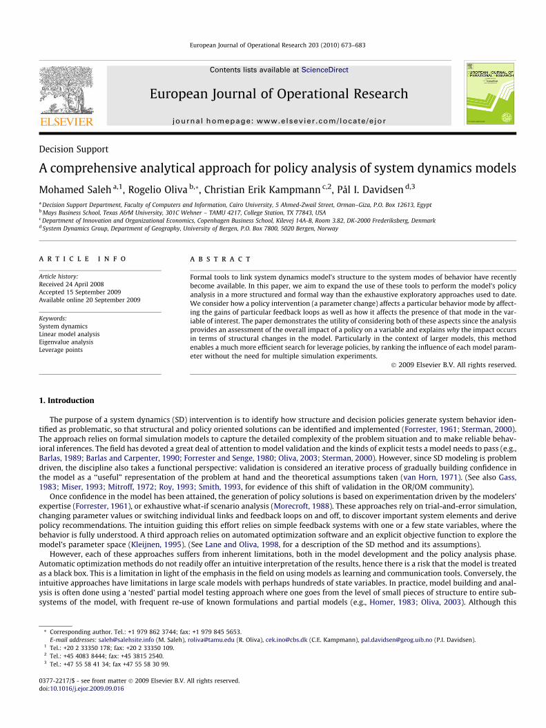
Fig. 1. Schematic representation of analytical process.

674 M. Saleh et al. / European Journal of Operational Research 203 (2010) 673–683

approach does carry a long way, it can be very difficult to discover feedback mechanisms that transcend model substructures in ways notanticipated by the modeler in the original dynamic hypothesis. In addition to being time consuming, the approach therefore carries thedanger that observed behavior is falsely attributed to certain feedback mechanisms when in fact another set of feedbacks is driving theoutcome, and the derived policy recommendations might be counterproductive. Clearly, a more rigorous theory for the link between feed-back structure and behavior in general large-scale systems would be of great value.

Recently, formal tools to articulate precise theories in SD models have become available (see Kampmann and Oliva, 2008, 2009, for areview of this literature). This work has focused on linking model structure to the system modes of behavior, expressed as the eigenvaluesof the linearized model.4 In particular, in what has been dubbed loop eigenvalue elasticity analysis (LEEA), the work has shown that there is aclose relationship between behavior modes and the strength of feedback loops, so that one may decompose the effects of structural changes interms of individual feedback loop contributions (see Kampmann, 1996; Kampmann and Oliva, 2006).

In this paper, we aim to expand the use of these formal tools to perform structured policy analysis. So far, little effort has been devotedto exploring the use of these tools for policy design. In part, this may be due to the computational intensity required to perform the analysisand the lack of integration of the method into mainstream modeling tools. Beyond these technical challenges, however, it has been difficultto interpret the results because eigenvalues define the characteristics of the system’s behavior modes (e.g., exponential growth, exponen-tial decay, expanding oscillations, damped oscillations), but these behavior modes are not equally manifested in the time path of a partic-ular model variable, making it difficult to link the eigenvalue analysis directly to the observed simulated behavior (Kampmann and Oliva,2006). We argue that for policy analysis, it is also necessary to consider this latter aspect.

Linear systems theory demonstrates how the behavior of a given variable can be expressed as a weighted sum of all the system behaviormodes. The weights, which we have dubbed dynamic decomposition weights (DDW), determine the manifestation of a particular behaviormode in the variable of interest and are related to the system eigenvectors and the current state of the model. Note that the term ‘‘dynamic”refers to the fact that the value of a weight changes as the state of the model changes. This is a manifestation of the fact that, even in linearmodels, in the transient phase, the contributions of the various modes of behavior to the total behavior evolve with time.

A number of SD scholars have indeed begun to consider the relative weights of behavior modes in specific system variables (see, e.g.,Gonçalves, 2009; Güneralp, 2006; Saleh, 2002; Saleh et al., 2005). The innovation of the present paper is twofold. First, we demonstratehow the dynamic decomposition weights analysis (DDWA) and the LEEA in a way are complements to each other. While LEEA is concernedwith changing the eigenvalues, DDWA is concerned with enhancing or suppressing the behavior modes for particular system variables.Second, we explicitly link the enhancement (or suppression) of behavior modes in system variables to policy design. We explore the policydesign space by assessing the elasticity of the presence behavior modes to changes in system parameters.

The paper is structured as follows. In Section 2, we outline the analytical framework, with most emphasis on the DDW analysis (sinceLEEA is well documented in previous work) and the link to policy analysis and model testing. In Section 3 we explore how the methodapplies to a simple inventory-workforce model (Sterman, 2000), which aims to provide an endogenous explanation of inventory and pro-duction oscillations in a manufacturing setting, beginning with a discussion of the significance of oscillation as a general problem phenom-enon and the ways one might formalize policy criteria for improvement. The analysis not only shows the impact of parameter changes onbehavior modes and weights, but it also shows how the LEEA/DDWA methods can aid an understanding of why the policy changes have theeffect they do. We conclude the paper with reflections on the general utility of the method. The mathematical results underlying the ap-proach are either documented in previous work or they are standard results from linear systems theory. The reader is referred to the on-line Appendix listed at the end of the paper for details of the derivations.

2. Analytical framework

A schematic representation of the analytical framework is provided in Fig. 1. The aim of the analysis is to provide an understanding ofthe link between three elements: the model structure, the policy parameters in the model, and the resulting time behavior of key systemvariables of interest (the three oval items in Fig. 1). As the figure further indicates, the method involves three analytical components: lin-earization of the model, LEE analysis, and DDW analysis. These three components complement each other and provide the basis for a cir-cular process of model testing, policy analysis, and policy interpretation for implementation.

4 In the following, we shall be somewhat informal in using the terms behavior mode and eigenvalue interchangeably. Strictly speaking, though, the eigenvalue k corresponds tothe behavior mode ekt .

M. Saleh et al. / European Journal of Operational Research 203 (2010) 673–683 675

2.1. Linearization

Mathematically, a system dynamics model is a set of nonlinear ordinary differential equations. One may approximate the model arounda particular point in time t0 by a set of time-invariant linear differential equations

_xðtÞ ¼ GxðtÞ þ BuðtÞ þ bxðt0Þ ¼ x0;

ð1Þ

where x; u are column vectors of the n state variables (levels), and p exogenous variables, respectively, _x is the vector of first time derivatives(rates), t is the simulated time, G and B are constant matrices, and b a constant vector of the appropriate dimension (see, e.g., Diallo and Rahn,1990). The LEE and DDW analyses are both based upon this linearized system. Since the main aim of our analysis is initially concerned withthe endogenous response of the system, we focus here on the endogenous dynamics by assuming that the exogenous variables are zero orconstant ðuðtÞ ¼ 0Þ. (See Kampmann and Oliva, 2006, for a discussion of when such an approximation is appropriate and useful).

In the absence of changes in exogenous inputs, the resulting behavior of any given state variable xðtÞ can be written as a weighted sumof a set of behavior modes,

xðtÞ ¼ w0 þw1ek1t þ � � � þwneknt; ð2Þ

where the ks are the eigenvalues of the system Jacobian matrix G, expressed by the characteristic polynomial PðkÞ ¼ detðkI� GÞ ¼ 0, and theweights w are a function of the eigenvectors of G and the vector b in (1) (Chen, 1970). For real eigenvalues, the behavior mode ekt amounts toan exponential growth ðk > 0Þ or adjustment ðk < 0Þ. Complex eigenvalues appear in conjugate pairs d� ix, leading to terms of the formedt sinðxt þ hÞ, corresponding to expanding or damped oscillations (if d > 0 or d < 0, respectively). The weights w determine how much eachof these modes is expressed in a particular system variable.

2.2. Loop eigenvalue elasticity analysis

The Loop Eigenvalue Elasticity Analysis, LEEA, is concerned with what happens to an eigenvalue k when one changes individual ele-ments g of the matrix G in (1), often measured as the eigenvalue elasticity, e ¼ ð@k=@gÞðg=kÞ. A theorem known as Mason’s Rule showshow the coefficients of PðkÞ can be interpreted as gains of feedback loops (measured as the product of the gains of the links constitutingthe loops), i.e., there is a one-to-one correspondence between loop gains and eigenvalues. In particular, changes in relationships in themodel that are not part of a feedback loop will have no effect upon the system eigenvalues. Kampmann (1996) pointed out a problemin this interpretation: that a given system may potentially contain very large number of feedback loops. Using graph theory, he showedhow one can focus on a much smaller subset of independent feedback loops that still capture the full feedback complexity of the systemand support a computation of the loop eigenvalue elasticity. The analysis, therefore, supports an interpretation of the relative importanceof particular feedback loops in generating a particular mode of behavior, where loops with large elasticities are considered importantfor the behavior mode in question. Oliva (2004) and Oliva and Mojtahedzadeh (2004) showed how choosing the shortest independent loopsets allows for relatively more intuitive interpretation of the loops.

2.3. Dynamic decomposition weight analysis

The Dynamic Decomposition Weight Analysis, DDWA, is concerned with what happens to the weights w in (2) when changes aremade to the system elements. In contrast to LEEA, all the links in the model are potentially relevant in DDWA. Furthermore, the weightsare specific to each output variable of interest as well as the current state of the system (the reference point from which the lineariza-tion is made).

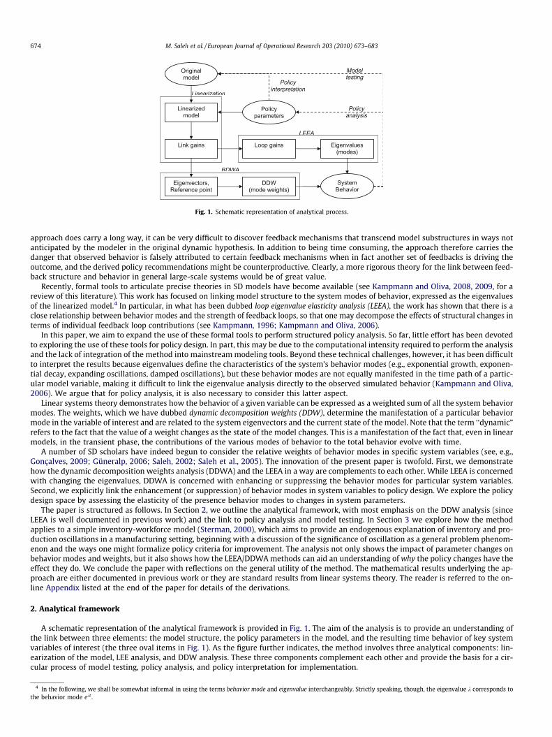
The pseudo-code for the DDW algorithm is listed in Fig. 2. The algorithm consists of two loops. The outer loop traverses the time horizonof the study with a time step s – that is, the computations are performed at regular intervals of length s. First, the values of the state vari-ables are obtained from the simulation data and then the Weights function is called to generate the base values for the eigenvalue vector k�

and the weights matrix W�. These values are derived from the values of the elements of G, which in turn are computed from the currentvalues of the state variables and parameters, and b. Once the base values are computed, in the inner loop each parameter in p (one at atime) is slightly perturbed to numerically compute the eigenvalue and weight elasticities, by comparing the new values to the base case.Once the computations have been performed, the analysis is based on the manipulation and interpretation of the output variables Ek andEw. Depending upon the degree of nonlinearity in the model, the analysis should be performed at several points along the simulated tra-jectory of the model. (Kampmann and Oliva (2006) discuss the merits of using linear analysis in nonlinear models).

2.3.1. Behavior decompositionAs a first step, it is possible to assess the projection of each of the reference modes in each state variable by expressing the time trajec-

tory of the state variables in the form of Eq. (2). This representation immediately reveals the duration and intensity of the projection of eacheigenvalue in the overall behavior of the state variable. This representation helps focus the analysis to the behavior patterns that need to beaddressed – either to increase or decrease their projection depending on whether the behavior pattern is desirable or not.

2.3.2. Policy (parameter) analysisThe method then proceeds to policy analysis by considering how specific interventions (parameter changes) in the model affect the sys-

tem’s response. An exploration of the policy design space can be achieved by assessing the influence of model parameters on the dynamicdecomposition weights. By focusing on the weights of the behavior modes for the variable of interest we can identify leverage points toincrease or decrease the influence of a behavior mode on the variable. While changes to model parameters might influence several statevariables simultaneously, parameters reflect policies and various ‘‘physical” realities in the system and as such represent intuitive inter-vention points. By assessing the parameter influence, Ew, in the DDWs, it is possible to quickly identify scaling parameters (parameters

[Eλ, Ew] ←← DDW(G, p, b, SimData, ts, te, τ, δ) t ← ts initialize time tracker to start-time while t ≤ te while time tracker less or equal than end-time x ← SimData tes}t{ x to state of system at time t [λ*, W*] ← Weights(G(x, p), b) function call to obtain base eigenvalues and weights for j=1:length(p) for every parameter in p pr ← p initialize pr to p pr{j} ← (1+δ) p{j} modify parameter j by δ [λ, W] ← Weights(G(x, pr), b) function call to obtain eigenvalues and weights Eλ{j, t} ← δ-1(λ-λ*)./λ* store eigenvalue elasticity to parameter j at time t Ew{j, t} ← δ-1(W-W*)./W* store weight elasticity to parameter j at time t

end )rof(dnet ← t + τ increment time tracker by τ

end end (while) end

[λ, W] ← Weights (J, b)λ ← Eigenvalue(J etaluclac) eigenvalues

R ← Eigenvector(J) calculate right eigenvector matrix a ← R-1b calculate projection on the right eigenvectors

W ← (a./λ)*R calculate dynamic weight matrix end

where G(x, p) is a symbolic representation of the system’s Jacobian in terms of state variables x and parameters p; b is a constant vector associated with the linearized model; SimData is a matrix containing the simulated values of the n state variables across time; and δ is the perturbation parameter. λ and λ* are vectors of length n, and W and W* are matrices of dimension nxn. Elasticity matrices Eλ and Ew have two additional dimensions to store elasticities by parameter and time. * denotes the base case values; the symbol ./ indicates element-by-element division.

Fig. 2. Pseudo-code for DDWA algorithm (see online Appendix for details).

676 M. Saleh et al. / European Journal of Operational Research 203 (2010) 673–683

that affect the scale but not the behavior mode of state variables) and the parameters with high leverage on the desired (or undesired)reference modes.

Changes in parameters, however, not only impact the dynamic decomposition weights, but also change the eigenvalues themselves (ex-pressed by the measure Ek). This dual impact of parameter changes introduces a challenge in developing policy recommendations sincechanges not only affect the way a behavior mode is projected in the trajectory of a state variable, but also changes the behavior mode itself.

After completing the analysis for all state variables and time instants of interest, it is possible to generate a set of recommendations forthe policymaker in terms of changes in parameter values and explain the effects of these parameter changes by analyzing their roles inchanging the feedback structure with the help from the LEEA results. By referring back to the original model, the analyst is afforded a dee-per understanding of why the particular policy interventions work the way they do, which can be the basis of real-world interpretation andexplanation and model validation and testing.

Both the LEEA and DDWA methods have been implemented in Mathematica� routines and are available online (Oliva, 2009), along withthe example models in Vensim� and text parsing routines that generate the appropriate Mathematica� files from a Vensim� model file.

3. Analysis of a simple inventory-workforce model

In this section we apply the analytical framework to a simple system dynamics model of oscillations in a manufacturing system. Pro-duction and inventory oscillations and minimization of inventory carrying costs as well as adjustment costs in changing output are fre-quently studied in the OR/OM literature (e.g., Chandra and Grabis, 2005; Hoberg et al., 2007; Iglehart, 1963; Sterman, 1989). Thebenefit of an SD model to address this issue is the articulation of an endogenous explanation for these oscillations, i.e., an explanationin terms of variables that are under management control. The formal analysis of the model that we propose here provides a rigorousand direct identification of the levers that are more significant for management purposes. Before proceeding to the analysis, we briefly dis-cuss criteria for successful policy changes.

3.1. Oscillation and policy criteria

Forrester (1982) discusses different measures of stabilizing policies and their possible tradeoffs. This issue, however, is difficult to treatin general, since the policy criteria are linked to the purpose of the model and the problem definition, which may involve transient behav-iors like overshoot and collapse – e.g., in the World model (Forrester, 1971) – or the settlement in the system to undesirable end states –e.g., in the Urban Dynamics model (Forrester, 1969). In this paper, we focus on policies that reduce the oscillatory tendencies of the system,since the model presented is designed to address this issue, and since, as was demonstrated by Kampmann and Oliva (2006), it appears tobe one of areas where the eigenvalue analysis shows the most promise.

As mentioned above, eigenvalues associated with oscillations appear as complex conjugate pairs d� ix. In the context of unwantedinstabilities (oscillations), effective policies are often defined as those that either increase the damping of oscillatory behavior modes bymaking the real part d more negative (the settling time criterion) or, when adjustment costs are significant, decrease the (damped) fre-quency of oscillation x (the frequency criterion). More general measures are based upon more sophisticated objective functions relatingto the ability of the system to absorb exogenous disturbances. Examples include the variance of a specific system variable or the fre-quency response of the variable. A summary of criteria is provided in Table 1. Since all of these measures are ultimately related tothe system eigenvalues and the DDW, we have chosen in this work to focus on these directly and relegate other measures to subsequentwork.

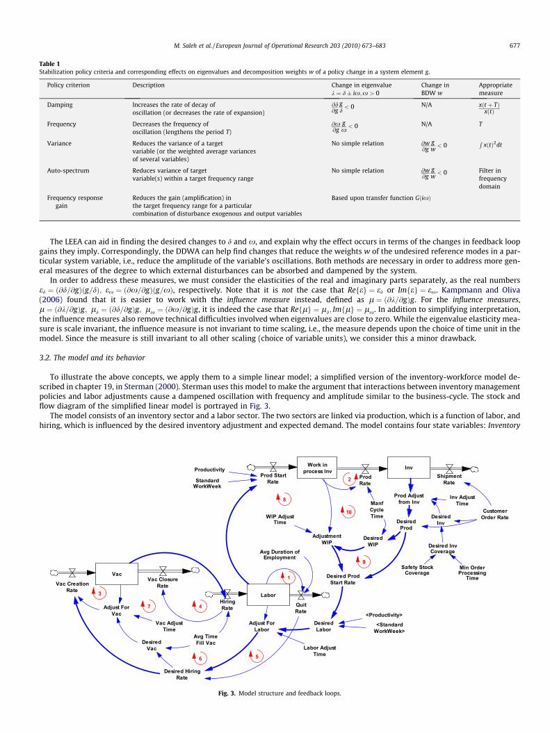
Table 1Stabilization policy criteria and corresponding effects on eigenvalues and decomposition weights w of a policy change in a system element g.

Policy criterion Description Change in eigenvaluek ¼ d� ix;x > 0

Change inBDW w

Appropriatemeasure

Damping Increases the rate of decay ofoscillation (or decreases the rate of expansion)

@d@g

gd< 0 N/A xðt þ TÞ

xðtÞ

Frequency Decreases the frequency ofoscillation (lengthens the period T)

@x@g

gx < 0 N/A T

Variance Reduces the variance of a targetvariable (or the weighted average variancesof several variables)

No simple relation @w@g

gw< 0

RxðtÞ2dt

Auto-spectrum Reduces variance of targetvariable(s) within a target frequency range

No simple relation @w@g

gw< 0 Filter in

frequencydomain

Frequency responsegain

Reduces the gain (amplification) inthe target frequency range for a particularcombination of disturbance exogenous and output variables

Based upon transfer function GðixÞ

M. Saleh et al. / European Journal of Operational Research 203 (2010) 673–683 677

The LEEA can aid in finding the desired changes to d and x, and explain why the effect occurs in terms of the changes in feedback loopgains they imply. Correspondingly, the DDWA can help find changes that reduce the weights w of the undesired reference modes in a par-ticular system variable, i.e., reduce the amplitude of the variable’s oscillations. Both methods are necessary in order to address more gen-eral measures of the degree to which external disturbances can be absorbed and dampened by the system.

In order to address these measures, we must consider the elasticities of the real and imaginary parts separately, as the real numbersed ¼ ð@d=@gÞðg=dÞ; ex ¼ ð@x=@gÞðg=xÞ, respectively. Note that it is not the case that Refeg ¼ ed or Imfeg ¼ ex. Kampmann and Oliva(2006) found that it is easier to work with the influence measure instead, defined as l ¼ ð@k=@gÞg. For the influence measures,l ¼ ð@k=@gÞg; ld ¼ ð@d=@gÞg; lx ¼ ð@x=@gÞg, it is indeed the case that Reflg ¼ ld; Imflg ¼ lx. In addition to simplifying interpretation,the influence measures also remove technical difficulties involved when eigenvalues are close to zero. While the eigenvalue elasticity mea-sure is scale invariant, the influence measure is not invariant to time scaling, i.e., the measure depends upon the choice of time unit in themodel. Since the measure is still invariant to all other scaling (choice of variable units), we consider this a minor drawback.

3.2. The model and its behavior

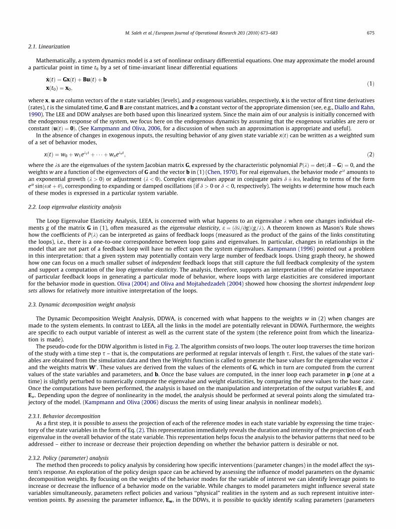
To illustrate the above concepts, we apply them to a simple linear model; a simplified version of the inventory-workforce model de-scribed in chapter 19, in Sterman (2000). Sterman uses this model to make the argument that interactions between inventory managementpolicies and labor adjustments cause a dampened oscillation with frequency and amplitude similar to the business-cycle. The stock andflow diagram of the simplified linear model is portrayed in Fig. 3.

The model consists of an inventory sector and a labor sector. The two sectors are linked via production, which is a function of labor, andhiring, which is influenced by the desired inventory adjustment and expected demand. The model contains four state variables: Inventory

Work inprocess Inv

Prod StartRate

ProdRate

InvShipment

Rate

Productivity

AdjustmentWIP

Desired ProdStart Rate

DesiredProd

CustomerOrder RateDesired

Inv

Desired InvCoverage

Min OrderProcessing

Time

Safety StockCoverage

ManfCycleTime

DesiredWIP

WIP AdjustTime

Inv AdjustTime

Prod Adjustfrom Inv

StandardWorkWeek

2

8

9

10

Vac

Labor

Vac CreationRate

Vac ClosureRate

HiringRate Quit

Rate

Avg Duration ofEmployment

Adjust ForLabor

Labor AdjustTime

Desired HiringRate

DesiredLabor

Adjust ForVac

Vac AdjustTime

DesiredVac

Avg TimeFill Vac

<StandardWorkWeek>

<Productivity>

1

3

4

56

7

Fig. 3. Model structure and feedback loops.

-0.04

-0.03

-0.02

-0.01

0.00

0.01

0.02

0.00 0.01 0.02 0.03 0.04

Re[

μ]

Abs[μ]

1

9

5

10

4

2

8

3,7

6

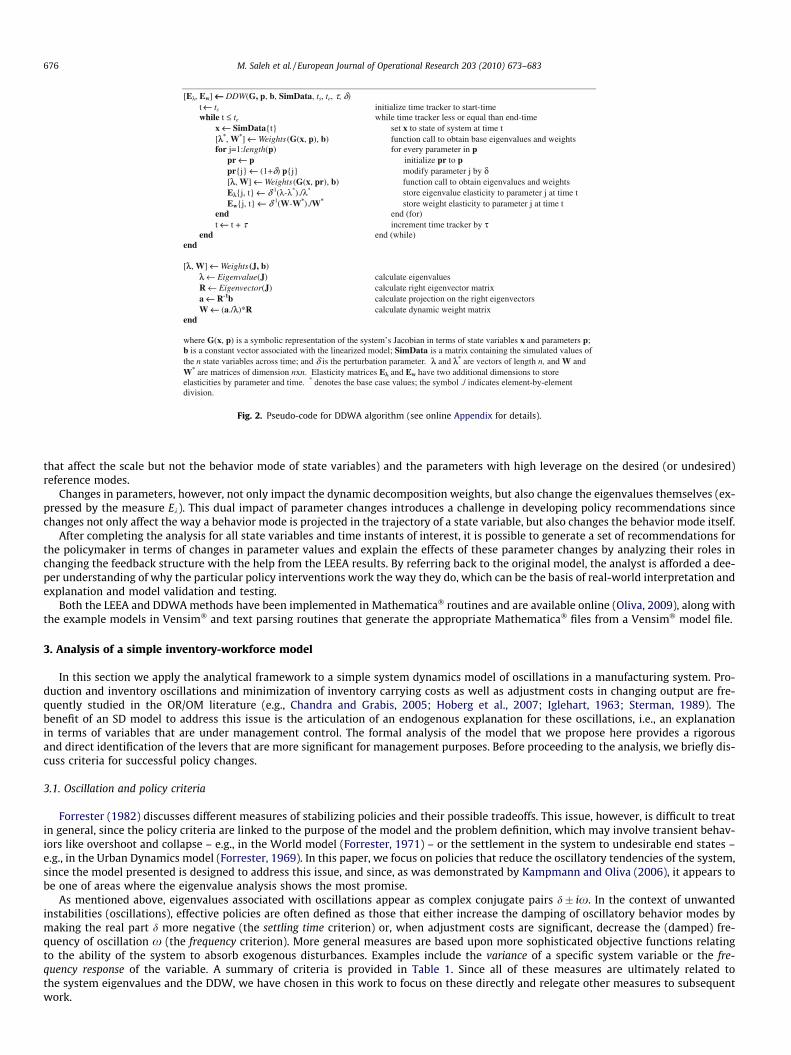
Fig. 4. Loop influence on the oscillatory behavior mode.

Fig. 5. State variable behavior decomposition.

678 M. Saleh et al. / European Journal of Operational Research 203 (2010) 673–683

(Inv), Labor, Vacancies (Vac), and Work in Process Inventory (WIP). The behavior of these state variables is illustrated in Fig. 5 (bold lines),showing a 200 week simulation of the model which is initialized out of equilibrium but is otherwise undisturbed by exogenous variables.The most salient behavior is an oscillation with a period of approximately 65 months (see also the Base run in Fig. 6).

The causal explanation of the oscillation is well known from elementary SD. The key factor leading to oscillation is the delay involved inadjusting production by hiring or firing labor. For instance, if there is excess inventory, production must be reduced below shipments tobring down inventory, i.e., labor must be brought below its equilibrium value. However, as inventory falls and reaches its equilibrium va-lue, the policies implemented in the model imply that the labor stock is now too low. Thus inventory continues to fall below the equilib-rium level, leading to net hiring of labor, which, after a delay, reverses the cycle (see Sterman, 2000, Chapter 19).

The four state variables give rise to four eigenvalues or behavior modes, listed in Table 2. Because the model is linear, the eigenvalues donot change over time. Two of the eigenvalues are real, corresponding to exponential adjustment behavior modes with an adjustment timeof approximately 3 weeks and 7 weeks, respectively. The two remaining eigenvalues form a complex conjugate pair, leading to a dampedoscillatory mode with an adjustment time of about 106 weeks and a period of about 64 weeks. As is evident from Fig. 5, the oscillatory

Table 2Behavior modes k of Inventory (Inv).

Mode k Unit k1 k2 k3; k4

Real part Refkg 1/week �0.353 �0.138 �0.0095Imaginary part Imfkg 1/week 0.000 0.000 0.0988Exp. adj. time s ¼ 1=Refkg weeks �2.832 �7.246 �105.236Oscillation period T ¼ 2p=Imfkg weeks � � 63.595

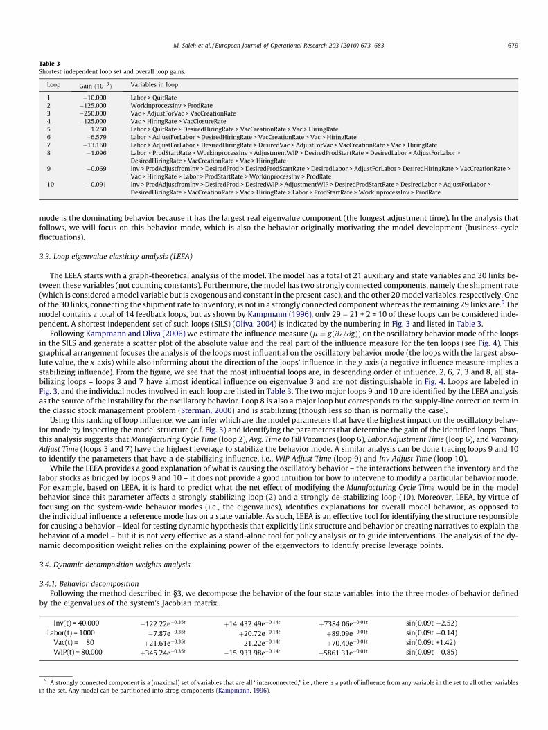
Table 3Shortest independent loop set and overall loop gains.

Loop Gain ð10�3Þ Variables in loop

1 �10.000 Labor > QuitRate2 �125.000 WorkinprocessInv > ProdRate3 �250.000 Vac > AdjustForVac > VacCreationRate4 �125.000 Vac > HiringRate > VacClosureRate5 1.250 Labor > QuitRate > DesiredHiringRate > VacCreationRate > Vac > HiringRate6 �6.579 Labor > AdjustForLabor > DesiredHiringRate > VacCreationRate > Vac > HiringRate7 �13.160 Labor > AdjustForLabor > DesiredHiringRate > DesiredVac > AdjustForVac > VacCreationRate > Vac > HiringRate8 �1.096 Labor > ProdStartRate > WorkinprocessInv > AdjustmentWIP > DesiredProdStartRate > DesiredLabor > AdjustForLabor >

DesiredHiringRate > VacCreationRate > Vac > HiringRate9 �0.069 Inv > ProdAdjustfromInv > DesiredProd > DesiredProdStartRate > DesiredLabor > AdjustForLabor > DesiredHiringRate > VacCreationRate >

Vac > HiringRate > Labor > ProdStartRate > WorkinprocessInv > ProdRate10 �0.091 Inv > ProdAdjustfromInv > DesiredProd > DesiredWIP > AdjustmentWIP > DesiredProdStartRate > DesiredLabor > AdjustForLabor >

DesiredHiringRate > VacCreationRate > Vac > HiringRate > Labor > ProdStartRate > WorkinprocessInv > ProdRate

M. Saleh et al. / European Journal of Operational Research 203 (2010) 673–683 679

mode is the dominating behavior because it has the largest real eigenvalue component (the longest adjustment time). In the analysis thatfollows, we will focus on this behavior mode, which is also the behavior originally motivating the model development (business-cyclefluctuations).

3.3. Loop eigenvalue elasticity analysis (LEEA)

The LEEA starts with a graph-theoretical analysis of the model. The model has a total of 21 auxiliary and state variables and 30 links be-tween these variables (not counting constants). Furthermore, the model has two strongly connected components, namely the shipment rate(which is considered a model variable but is exogenous and constant in the present case), and the other 20 model variables, respectively. Oneof the 30 links, connecting the shipment rate to inventory, is not in a strongly connected component whereas the remaining 29 links are.5 Themodel contains a total of 14 feedback loops, but as shown by Kampmann (1996), only 29 � 21 + 2 = 10 of these loops can be considered inde-pendent. A shortest independent set of such loops (SILS) (Oliva, 2004) is indicated by the numbering in Fig. 3 and listed in Table 3.

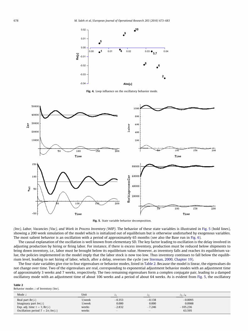
Following Kampmann and Oliva (2006) we estimate the influence measure ðl ¼ gð@k=@gÞÞ on the oscillatory behavior mode of the loopsin the SILS and generate a scatter plot of the absolute value and the real part of the influence measure for the ten loops (see Fig. 4). Thisgraphical arrangement focuses the analysis of the loops most influential on the oscillatory behavior mode (the loops with the largest abso-lute value, the x-axis) while also informing about the direction of the loops’ influence in the y-axis (a negative influence measure implies astabilizing influence). From the figure, we see that the most influential loops are, in descending order of influence, 2, 6, 7, 3 and 8, all sta-bilizing loops – loops 3 and 7 have almost identical influence on eigenvalue 3 and are not distinguishable in Fig. 4. Loops are labeled inFig. 3, and the individual nodes involved in each loop are listed in Table 3. The two major loops 9 and 10 are identified by the LEEA analysisas the source of the instability for the oscillatory behavior. Loop 8 is also a major loop but corresponds to the supply-line correction term inthe classic stock management problem (Sterman, 2000) and is stabilizing (though less so than is normally the case).

Using this ranking of loop influence, we can infer which are the model parameters that have the highest impact on the oscillatory behav-ior mode by inspecting the model structure (c.f. Fig. 3) and identifying the parameters that determine the gain of the identified loops. Thus,this analysis suggests that Manufacturing Cycle Time (loop 2), Avg. Time to Fill Vacancies (loop 6), Labor Adjustment Time (loop 6), and VacancyAdjust Time (loops 3 and 7) have the highest leverage to stabilize the behavior mode. A similar analysis can be done tracing loops 9 and 10to identify the parameters that have a de-stabilizing influence, i.e., WIP Adjust Time (loop 9) and Inv Adjust Time (loop 10).

While the LEEA provides a good explanation of what is causing the oscillatory behavior – the interactions between the inventory and thelabor stocks as bridged by loops 9 and 10 – it does not provide a good intuition for how to intervene to modify a particular behavior mode.For example, based on LEEA, it is hard to predict what the net effect of modifying the Manufacturing Cycle Time would be in the modelbehavior since this parameter affects a strongly stabilizing loop (2) and a strongly de-stabilizing loop (10). Moreover, LEEA, by virtue offocusing on the system-wide behavior modes (i.e., the eigenvalues), identifies explanations for overall model behavior, as opposed tothe individual influence a reference mode has on a state variable. As such, LEEA is an effective tool for identifying the structure responsiblefor causing a behavior – ideal for testing dynamic hypothesis that explicitly link structure and behavior or creating narratives to explain thebehavior of a model – but it is not very effective as a stand-alone tool for policy analysis or to guide interventions. The analysis of the dy-namic decomposition weight relies on the explaining power of the eigenvectors to identify precise leverage points.

3.4. Dynamic decomposition weights analysis

3.4.1. Behavior decompositionFollowing the method described in §3, we decompose the behavior of the four state variables into the three modes of behavior defined

by the eigenvalues of the system’s Jacobian matrix.

in

Inv(t) = 40,000

5 A strongly connected componentthe set. Any model can be partitio

�122:22e�0:35t

is a (maximal) set of variablesned into strog components (K

þ14;432:49e�0:14t

that are all ‘‘interconnected,” i.e., thampmann, 1996).

þ7384:06e�0:01t

ere is a path of influence from a

sin(0.09t �2.52)

Labor(t) = 1000 �7:87e�0:35t þ20:72e�0:14t þ89:09e�0:01t sin(0.09t �0.14)

Vac(t) = 80

þ21:61e�0:35t �21:22e�0:14t þ70:40e�0:01t sin(0.09t +1.42) WIP(t) = 80,000 þ345:24e�0:35t �15;933:98e�0:14t þ5861:31e�0:01t sin(0.09t �0.85)

ny variable in the set to all other variables

Table 4Behavior decomposition weights for the four state variables xiðtÞ ¼ ui þw1 expðk1tÞ þw2 expðk2tÞ þw3 expðRe½k3 �tÞ sinðIm½k3 �t þ hiÞ.

Variable xðtÞ Inv Labor Vac WIP

Constant u 40,000 1000 80 80,000Weight w1 �122.22 �7.87 21.61 345.24Weight w2 14,432.49 20.72 �21.22 �15,933.98Weight w3 7384.06 89.09 70.40 5861.31h �2.52 �0.14 1.42 �0.85w1=u �0.003 �0.007 0.270 0.004w2=u 0.361 0.021 �0.265 �0.199w3=u 0.185 0.089 0.880 �0.073

680 M. Saleh et al. / European Journal of Operational Research 203 (2010) 673–683

Table 4 presents the decomposition weights in a matrix format and also shows the phase lag expressed in radians as well as the weightsnormalized by the constant term. The decomposition of the behavior of the state variables can be observed in Fig. 5. In each panel of thefigure, the four components of behavior (three behavior modes plus the steady-state constant) have been plotted with a thin line and theoverall behavior of the variable – the addition of the four components – with a broader line. With the exception of Vacancies, the compo-nent from behavior mode 1 is hardly visible in these plots, which is confirmed by normalizing the decomposition equations with the stea-dy-state constant, c.f. Table 4.

From the scaled weights and the corresponding plots in Fig. 5, it is relatively easy to perform a set of diagnostics. First, modes one andtwo represent rapid adjustments at the beginning of the simulation. Note that those two modes have little or no impact on those variablesthat started the simulation close to their steady-state value, e.g., labor. Relatively quickly, these modes die out and the variable behavior iscontrolled by the damped oscillation of mode three. Second, all variables are oscillating with the same frequency, corresponding to mode 3,i.e., with a period of around 63 weeks, but with different phasing; h values (measured in radians) range from �2.52 to 1.42, representing a225� phase lag between inventory and vacancies.

Focusing on inventory, for example, we see that w2 (the weight of the second eigenvalue) is much larger than the other two weights oninventory. Indeed, Fig. 5 reveals that, while significant, the second behavior mode is only active during the first 25 simulation periods. Afterperiod 25, the whole behavior of the inventory variable is dominated by the third behavior mode.

3.4.2. Parameter analysisThe parameter analysis assesses the influence of model parameters on the dynamic decomposition weights. By focusing on the weights

of the behavior modes on the variable of interest it is possible to identify policy levers that will have the desired impact on the systembehavior. The Weight elasticity column in Table 5 reports the parameter elasticity of w3 (the weight of eigenvalue 3, the oscillatory behaviormode) on Inventory ðe ¼ ð@w=@pÞðp=wÞÞ. The magnitude of the elasticity quantifies the impact that changes in the parameter value have onthe weight of the oscillatory behavior mode on Inventory. To facilitate the analysis, the table is sorted in descending order of absolute valueof elasticity.

A positive weight elasticity measure in Table 5 indicates that an increase in the parameter value will increase the weight of the oscil-latory behavior mode in the trajectory of the Inventory state variable. Alternatively, a negative influence measure means that increasing theparameter value will reduce the projection of the oscillatory behavior mode on the behavior of Inventory. Fig. 6 illustrates the impact onInventory of a 5% increase in the values of the Customer Order Rate and Productivity. Note that relative to the base case, increasing the Cus-tomer Order Rate increases the projection of the oscillatory mode on Inventory, i.e., Inventory shows a greater amplitude – as expected fromthe large positive influence measure reported for that parameter in Table 5 – but it does not affect the period and damping ratio of theoscillation. Consistent with a negative influence and of smaller magnitude (c.f. Table 4), a 5% increase in the Productivity parameter reducesamplitude of the Inventory oscillations while maintaining the frequency and settling time of the oscillatory mode.

To facilitate assessing the dual impact of parameter changes discussed above (impact on the dynamic decomposition weights and theeigenvalues), the last two columns of Table 5 report the influence on the eigenvalue (real and imaginary part) for each parameter. Thesemeasures of influence should be interpreted in a similar way as the weight elasticities.

Note in Table 5 that several model parameters (Customer Order Rate, Productivity, Standard Work Week, Safety Stock Coverage, and Min-imum Order Processing Time) have no influence on the oscillatory behavior mode. Three of these parameters (Customer Order Rate, SafetyStock Coverage, and Minimum Order Processing Time) are not affecting directly any of the links within the system’s feedback loops and, whilechanges in these parameters will have an impact on the weights on the state variables, they do not affect the relative underlying oscillatory

Table 5Elasticity to parameters of weight of eigenvalue 3 on Inventory and influence of parameters on eigenvalue 3.

Parameter w3 on Inv elasticity Influence on Re[k3] Influence on Im½k3�

Customer order rate 16.271 0.000 0.000Manufacturing cycle time 7.558 0.019 0.010Productivity �2.997 0.000 0.000Standard work week �2.997 0.000 0.000Safety stock coverage 2.280 0.000 0.000Min order processing time 2.280 0.000 0.000Inventory adjustment time 0.978 �0.034 �0.025Labor adjustment time 0.214 0.011 �0.049Vacancy adjustment time �0.077 0.009 0.000WIP adjustment time �0.063 0.000 �0.035Avg time to fill vacancies �0.032 0.004 0.000Avg duration of employment �0.012 0.000 0.001

30.000

35.000

40.000

45.000

50.000

55.000

60.000

0 50 100 150 200In

ven

tory

Months

Base

5% increase onProductivity

5% increase onCustomer Order Rate

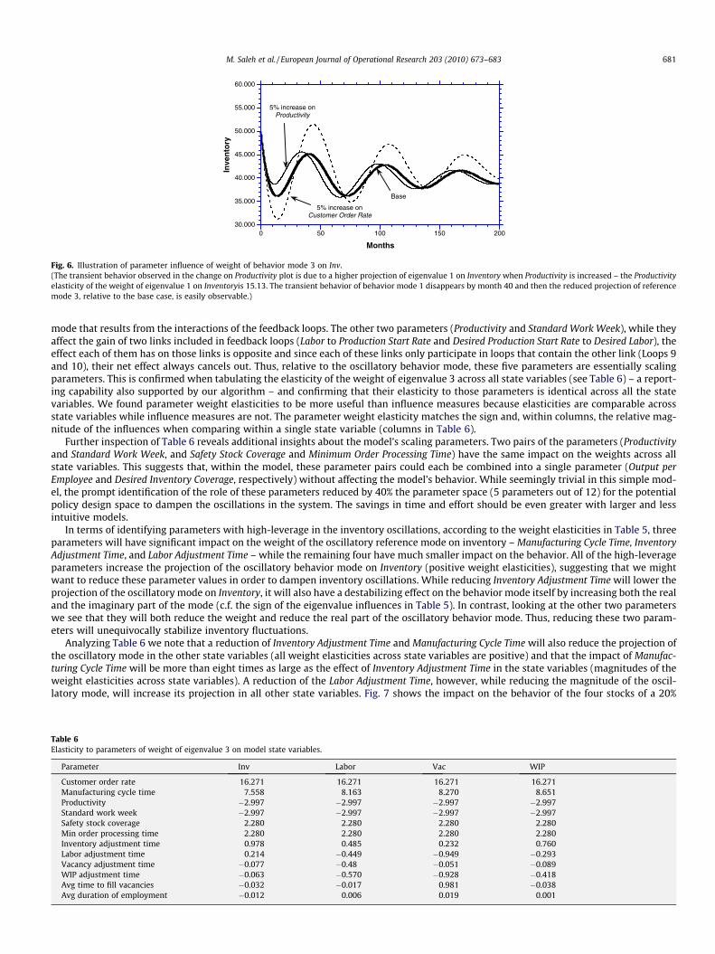
Fig. 6. Illustration of parameter influence of weight of behavior mode 3 on Inv.(The transient behavior observed in the change on Productivity plot is due to a higher projection of eigenvalue 1 on Inventory when Productivity is increased – the Productivityelasticity of the weight of eigenvalue 1 on Inventoryis 15.13. The transient behavior of behavior mode 1 disappears by month 40 and then the reduced projection of referencemode 3, relative to the base case, is easily observable.)

M. Saleh et al. / European Journal of Operational Research 203 (2010) 673–683 681

mode that results from the interactions of the feedback loops. The other two parameters (Productivity and Standard Work Week), while theyaffect the gain of two links included in feedback loops (Labor to Production Start Rate and Desired Production Start Rate to Desired Labor), theeffect each of them has on those links is opposite and since each of these links only participate in loops that contain the other link (Loops 9and 10), their net effect always cancels out. Thus, relative to the oscillatory behavior mode, these five parameters are essentially scalingparameters. This is confirmed when tabulating the elasticity of the weight of eigenvalue 3 across all state variables (see Table 6) – a report-ing capability also supported by our algorithm – and confirming that their elasticity to those parameters is identical across all the statevariables. We found parameter weight elasticities to be more useful than influence measures because elasticities are comparable acrossstate variables while influence measures are not. The parameter weight elasticity matches the sign and, within columns, the relative mag-nitude of the influences when comparing within a single state variable (columns in Table 6).

Further inspection of Table 6 reveals additional insights about the model’s scaling parameters. Two pairs of the parameters (Productivityand Standard Work Week, and Safety Stock Coverage and Minimum Order Processing Time) have the same impact on the weights across allstate variables. This suggests that, within the model, these parameter pairs could each be combined into a single parameter (Output perEmployee and Desired Inventory Coverage, respectively) without affecting the model’s behavior. While seemingly trivial in this simple mod-el, the prompt identification of the role of these parameters reduced by 40% the parameter space (5 parameters out of 12) for the potentialpolicy design space to dampen the oscillations in the system. The savings in time and effort should be even greater with larger and lessintuitive models.

In terms of identifying parameters with high-leverage in the inventory oscillations, according to the weight elasticities in Table 5, threeparameters will have significant impact on the weight of the oscillatory reference mode on inventory – Manufacturing Cycle Time, InventoryAdjustment Time, and Labor Adjustment Time – while the remaining four have much smaller impact on the behavior. All of the high-leverageparameters increase the projection of the oscillatory behavior mode on Inventory (positive weight elasticities), suggesting that we mightwant to reduce these parameter values in order to dampen inventory oscillations. While reducing Inventory Adjustment Time will lower theprojection of the oscillatory mode on Inventory, it will also have a destabilizing effect on the behavior mode itself by increasing both the realand the imaginary part of the mode (c.f. the sign of the eigenvalue influences in Table 5). In contrast, looking at the other two parameterswe see that they will both reduce the weight and reduce the real part of the oscillatory behavior mode. Thus, reducing these two param-eters will unequivocally stabilize inventory fluctuations.

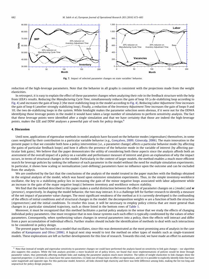
Analyzing Table 6 we note that a reduction of Inventory Adjustment Time and Manufacturing Cycle Time will also reduce the projection ofthe oscillatory mode in the other state variables (all weight elasticities across state variables are positive) and that the impact of Manufac-turing Cycle Time will be more than eight times as large as the effect of Inventory Adjustment Time in the state variables (magnitudes of theweight elasticities across state variables). A reduction of the Labor Adjustment Time, however, while reducing the magnitude of the oscil-latory mode, will increase its projection in all other state variables. Fig. 7 shows the impact on the behavior of the four stocks of a 20%

Table 6Elasticity to parameters of weight of eigenvalue 3 on model state variables.

Parameter Inv Labor Vac WIP

Customer order rate 16.271 16.271 16.271 16.271Manufacturing cycle time 7.558 8.163 8.270 8.651Productivity �2.997 �2.997 �2.997 �2.997Standard work week �2.997 �2.997 �2.997 �2.997Safety stock coverage 2.280 2.280 2.280 2.280Min order processing time 2.280 2.280 2.280 2.280Inventory adjustment time 0.978 0.485 0.232 0.760Labor adjustment time 0.214 �0.449 �0.949 �0.293Vacancy adjustment time �0.077 �0.48 �0.051 �0.089WIP adjustment time �0.063 �0.570 �0.928 �0.418Avg time to fill vacancies �0.032 �0.017 0.981 �0.038Avg duration of employment �0.012 0.006 0.019 0.001

30.000

40.000

50.000

60.000

70.000

80.000

90.000

0 50 100 150 200

Units

Month

WIP

Inventory

20% reducion onManufacturing Cycle Time

Base

20% reducion onInventory Adjustment Time

0

200

400

600

800

1.000

1.200

0 50 100 150 200

Employees

Month

Labor

Vacancies

20% reducion onManufacturing Cycle Time

Base20% reducion onInventory Adjustment Time

Fig. 7. Impact of selected parameter changes on state variables’ behavior.

682 M. Saleh et al. / European Journal of Operational Research 203 (2010) 673–683

reduction of the high-leverage parameters. Note that the behavior in all graphs is consistent with the projections made from the weightelasticities.

In retrospect, it is easy to explain the effect of these parameter changes when analyzing their role in the feedback structure with the helpfrom LEEA’s results. Reducing the Manufacturing Cycle Time, simultaneously reduces the gain of loop 10 (a de-stabilizing loop according toFig. 4) and increases the gain of loop 2 (the most stabilizing loop in the model according to Fig. 4). Reducing Labor Adjustment Time increasesthe gain of loop 6 (another strongly stabilizing loop). Finally, a reduction of the Inventory Adjustment Time increases the gain of loops 9 and10; the two de-stabilizing loops in the system. While hindsight makes the parameter selection seem obvious, if it were not for the DDWAidentifying those leverage points in the model it would have taken a large number of simulations to perform sensitivity analysis. The factthat these leverage points were identified after a single simulation and that we have certainty that those are indeed the high-leveragepoints, makes the LEE and DDW analyses a powerful pair of tools for policy design.6

4. Discussion

Until now, applications of eigenvalue methods in model analysis have focused on the behavior modes (eigenvalues) themselves, in somecases weighted by their contribution to a particular variable behavior (e.g., Gonçalves, 2009; Güneralp, 2006). The main innovation in thepresent paper is that we consider both how a policy intervention (i.e., a parameter change) affects a particular behavior mode (by affectingthe gains of particular feedback loops) and how it affects the presence of the behavior mode in the variable of interest (by affecting par-ticular link gains). We believe that the paper demonstrates the utility of considering both these aspects since the analysis affords both anassessment of the overall impact of a policy on a variable and performance measure of interest and gives an explanation of why the impactoccurs, in terms of structural changes in the model. Particularly in the context of larger models, the method enables a much more efficientsearch for leverage policies by ranking the influence of each parameter in the model without the need for multiple simulation experiments.In particular, it shows how scaling or normalization (unit-defining) parameters have no influence upon the outcome and can be excludedfrom the analysis.

We are comforted by the fact that the conclusions of the analysis of the model treated in the paper matches with the findings obtainedin the original analysis of the model, which was based upon extensive simulation experiments. Thus, in the simple inventory-workforceoscillator, the key to a stabilizing policy lies in increasing the gain of the minor negative loops associated with labor adjustment whilean increase in the gain of the major negative loop(s) between inventory and workforce reduces stability.

We find that the method described in this paper makes a useful distinction between the effect of parameter changes on k (modes) and w(presence), respectively. In shaping the model behavior, the two may interact. It is a challenge left for further research to identify a measureof the net impact of parameter value changes. The most significant weakness of the method as it is currently developed is the confoundingof the effects of initial conditions and of structural changes in the model: the decomposition weights w are a function of both the structure(eigenvectors) and the initial conditions. To resolve this issue, it will be necessary to employ policy criteria that are more general thanchanges in a particular simulated trajectory, such as those listed in the bottom rows of Table 1.

Moreover, it must be recognized that this method facilitates a partial policy analysis in the sense that we study the effects of changingindividual policy parameters. One must recognize that in non-linear systems each such effect is typically conditioned by the values of otherparameters. Consequently, when synthesizing values changes in several parameters into a policy, then the effects will interact and differfrom a pure accumulation of individual effects. Further studies should include the identification of methods to deal with such interactionsto be considered in policy design.

The present paper has focused on a model that oscillates, since this was demonstrated as the most promising area of analysis in the casestudies of Kampmann and Oliva (2006). A logical next step would to test the method on other types of models such as single-transientmodels. These explorations are left as further developments for this line of research. Towards this end, we have made an effort to automate

6 Note that instead of weight and eigenvalue sensitivity to parameter changes we could have performed the analysis based on sensitivity to link gain changes – our algorithmalso supports this analysis. While the link analysis provides a more localized set of policy levers, we found that most implementations of policies would be done throughparameter values, thus potentially affecting multiple links and making the parameter analysis much more intuitive. The tables of weight elasticities to link changes show theexpected properties: (i) all links in a chain have the same elasticities, (ii) links out of loops have no effect on eigenvalues, and (iii) it is possible to explicitly identify links that havesame magnitude and opposite sign. For this particular model, however, all links showed high elasticity and there was little difference among links, making the list too long andunpractical for policy design purposes.

M. Saleh et al. / European Journal of Operational Research 203 (2010) 673–683 683

and carefully document the procedures used in the analysis and made them freely available for download in the hope that other research-ers will pick up the tools and experiment with them.

Appendix A. Supplementary data

Mathematical derivations associated with this article can be found, in the online version, at doi:10.1016/j.ejor.2009.09.016.

References

Barlas, Y., 1989. Multiple tests for validation of system dynamics type of simulation models. European Journal of Operational Research 42 (1), 59–87.Barlas, Y., Carpenter, S., 1990. Philosophical roots of model validation: Two paradigms. System Dynamics Review 6 (2), 148–166.Chandra, C., Grabis, J., 2005. Application of multi-steps forecasting for restraining the bullwhip effect and improving inventory performance under autoregressive demand.

European Journal of Operational Research 166 (2), 337–350.Chen, C.T., 1970. Introduction to Linear System Theory. Holt, Rinehart and Winston, New York.Diallo, A., Rahn, R.J., 1990. Direct linearization of system dynamics models. System Dynamics Review 6 (2), 214–218.Forrester, J.W., 1961. Industrial Dynamics. Productivity Press, Cambridge, MA.Forrester, J.W., 1969. Urban Dynamics. Productivity Press, Cambridge, MA.Forrester, J.W., 1971. World Dynamics. Productivity Press, Cambridge.Forrester, J.W., Senge, P.M., 1980. Tests for building confidence in system dynamics models. TIMS Studies in Management Science 14, 209–228.Forrester, N.A., 1982. Dynamic synthesis of basic macroeconomic policy: Implications for stabilization policy analysis. Ph.D. Thesis, Sloan School of Management, Mass. Inst. of

Technology, Cambridge, MA.Gass, S.I., 1983. Decision-aiding models: Validation, assessment and related issues for policy analysis. Operations Research 31 (4), 603–631.Gonçalves, P., 2009. Eigenvalue and eigenvector analysis of dynamic systems. System Dynamics Review 25 (1), 35–62.Güneralp, B., 2006. Towards coherent loop dominance analysis: Progress in eigenvalue elasticity analysis. System Dynamics Review 22 (3), 263–289.Hoberg, K., Bradley, J.R., Thonemann, U.W., 2007. Analyzing the effect of the inventory policy on order and inventory variability with linear control theory. European Journal of

Operational Research 176 (3), 1620–1642.Homer, J.B., 1983. Partial-model testing as a validation tool for system dynamics. In: Proceedings of the Int. System Dynamics Conference, System Dynamics Society: Chestnut

Hill, MA, pp. 920–932.Iglehart, D.L., 1963. Optimality of (s, s) policies in the infinite horizon dynamic inventory problem. Management Science 9 (2), 259–267.Kampmann, C.E., 1996. Feedback loop gains and system behavior (unpublished manuscript). In: Proceedings of the Int. System Dynamics Conference, System Dynamics

Society: Cambridge, MA, pp. 260–263 (summarized).Kampmann, C.E., Oliva, R., 2006. Loop eigenvalue elasticity analysis: Three case studies. System Dynamics Review 22 (2), 146–162.Kampmann, C.E., Oliva, R., 2008. Structural dominance analysis and theory building in system dynamics. Systems Research and Behavioral Science 25 (4), 505–519.Kampmann, C.E., Oliva, R., 2009. Analytical methods for structural dominance analysis in system dynamics. In: Meyers, R. (Ed.), Encyclopedia of Complexity and Systems

Science. Springer, New York, pp. 8948–8967.Kleijnen, J.P.C., 1995. Sensitivity analysis and optimization of system dynamics models: Regression analysis and statistical design of experiments. System Dynamics Review 11

(4), 275–288.Lane, D.C., Oliva, R., 1998. The greater whole: Towards a synthesis of system dynamics and soft systems methodology. European Journal of Operational Research 107 (1), 214–

235.Miser, H.J., 1993. A foundational concept of science appropriate for validation in operational research. European Journal of Operational Research 66 (2), 204–234.Mitroff, I., 1972. The myth of objectivity or why science needs a new psychology of science? Management Science 18 (10), B613–B618.Morecroft, J.D.W., 1988. System dynamics and microworlds for policymakers. European Journal of Operational Research 59 (1), 9–27.Oliva, R., 2003. Model calibration as a testing strategy for system dynamics models. European Journal of Operational Research 151 (3), 552–568.Oliva, R., 2004. Model structure analysis through graph theory: Partition heuristics and feedback structure decomposition. System Dynamics Review 20 (4), 313–336.Oliva, R., 2009. System dynamics resource page. <http://iops.tamu.edu/faculty/roliva/research/sd/>.Oliva, R., Mojtahedzadeh, M., 2004. Keep it simple: Dominance assessment of short feedback loops. In: Proceedings of the Int. System Dynamics Conference, System Dynamics

Society, Oxford, UK.Roy, B., 1993. Decision science or decision-aid science? European Journal of Operational Research 66 (2), 184–203.Saleh, M., 2002. The characterization of model behavior and its causal foundation. Ph.D. Thesis, Dept. of Information Science, University of Bergen, Bergen, Norway.Saleh, M.M., Davidsen, P.I., Bayoumi, K.A.H., 2005. A comprehensive eigenvalue analysis of system dynamics models. In: Proceedings of the Int. System Dynamics Conference,

The System Dynamics Society, Boston, p. 130.Smith, J.H., 1993. Modeling muddles: Validation beyond the numbers. European Journal of Operational Research 66 (2), 235–249.Sterman, J.D., 1989. Modeling managerial behavior: Misperceptions of feedback in a dynamic decision making experiment. Management Science 35 (3), 321–339.Sterman, J.D., 2000. Business dynamics: Systems thinking and modeling for a complex world. Irwin McGraw-Hill, Boston.van Horn, R.L., 1971. Validation of simulation results. Management Science 17 (5), 247–258.