A COMPARISON STUDY OF GRACE-BASED GROUNDWATER …

A COMPARISON STUDY OF GRACE-BASED GROUNDWATER MODELING FOR

DATA-RICH AND DATA-POOR REGIONS

A THESIS IN

Environmental and Urban Geosciences

Presented to the Faculty of the University of

Missouri-Kansas City in partial fulfillment of

the requirements for the degree

MASTER OF SCIENCE

By

ALLA SKASKEVYCH

B.S., Computer Environmental and Economic Monitoring

Sevastopol National University of Nuclear Energy and Industry, 2009

Kansas City, Missouri

2014

© 2014

ALLA SKASKEVYCH

ALL RIGHTS RESERVED

iii

A COMPARISON STUDY OF GRACE-BASED GROUNDWATER MODELING FOR

DATA-RICH AND DATA-POOR REGIONS

Alla Skaskevych, Candidate for the Master of Science Degree

University of Missouri-Kansas City, 2014

ABSTRACT

Gravity Recovery and Climate Experiment (GRACE) modeling in water resources is

an emerging field in hydrology. Investigation of groundwater change using remote sensing

data helps overcome data limitation at a regional scale. We present a GRACE modeling

approach to estimate the variations of groundwater for two case studies, the Upper

Mississippi Basin in the US as a relatively data-rich region and the Ngadda catchment of the

Lake Chad Basin in Africa as a data-poor region. It is critical to understand whether GRACE

data is capable of analyzing groundwater change in data-poor regions as much as in data-rich

regions.

The GRACE data is applied first to analyze groundwater changes at the Upper

Mississippi Basin, and compare it with ground truth data. The modeling conditions that affect

the model accuracy are soil moisture models, groundwater fluctuations in the monitoring

well, and the matter of the aquifer. The most successful GRACE modeling approach

determined the effect of soil moisture model and aquifer. The strong correlation of 86.1%

iv

and 73.4%, respectively, verifies a good match between GRACE-based and ground truth

time series.

After the successful modeling approach is verified for the data-rich region, the

technique was employed for the Ngadda Catchment of the Lake Chad Basin, as a data-poor

region, to analyze groundwater changes. We investigated the effect of soil moisture models,

scales, groundwater fluctuations in the individual cell, and the coverage area parameters in

the GRACE modeling for the data-poor region. The most successful GRACE modeling

approach determined the effect of soil moisture model.

v

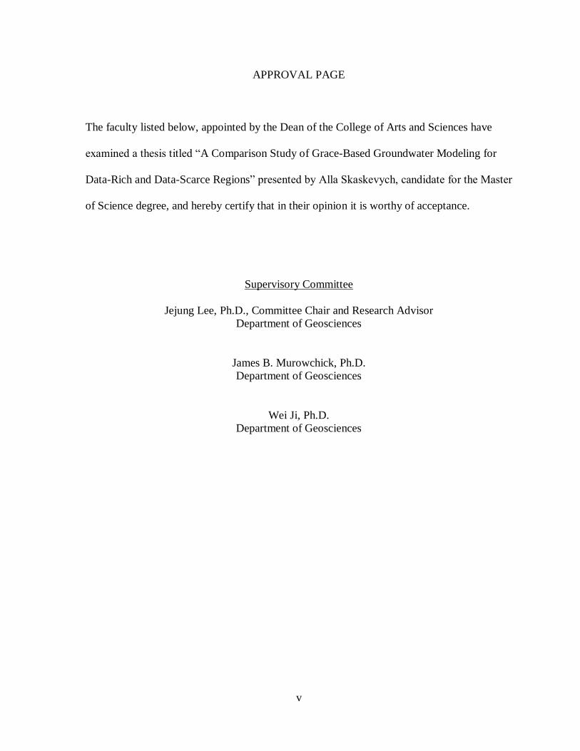
APPROVAL PAGE

The faculty listed below, appointed by the Dean of the College of Arts and Sciences have

examined a thesis titled “A Comparison Study of Grace-Based Groundwater Modeling for

Data-Rich and Data-Scarce Regions” presented by Alla Skaskevych, candidate for the Master

of Science degree, and hereby certify that in their opinion it is worthy of acceptance.

Supervisory Committee

Jejung Lee, Ph.D., Committee Chair and Research Advisor

Department of Geosciences

James B. Murowchick, Ph.D.


Wei Ji, Ph.D.


vi

CONTENTS

ABSTRACT ....................................................................................................................... .iii

ILLUSTRATIONS ............................................................................................................ viii

TABLES ............................................................................................................................ xi

ACKNOWLEDGEMENTS ............................................................................................... xii

Chapter

1. INTRODUCTION .......................................................................................................1

1.1 Statement of Problems .........................................................................................1

1.2 GRACE in General. .............................................................................................4

1.3 Lake Chad Basin ..................................................................................................6

1.4 Objectives .......................................................................................................... 10

2. LITERATURE REVIEW ........................................................................................... 12

2.1 Groundwater and Remote Sensing Studies for the Lake Chad Basin ................... 12

2.2 GRACE Modeling Studies for Groundwater ...................................................... 15

3. METHODOLOGY .................................................................................................... 18

3.1 Basic Theory of GRACE .................................................................................... 18

3.2 GLDAS in General ............................................................................................ 21

3.3 Implementation .................................................................................................. 24

3.3.1 Implementation of GRACE ....................................................................... 25

3.3.2 Implementation of GLDAS ....................................................................... 28

3.3.3 Groundwater Anomalies from the Ground-Truth Data ............................... 29

3.4 Statistical Analysis ............................................................................................. 30

4. RESULTS AND DISCUSSION ................................................................................. 33

4.1 Data-rich Region: Upper Mississippi Basin ........................................................ 33

vii

4.1.1 Effect of Soil Moisture Models .................................................................. 37

4.1.2 Effect of Groundwater Fluctuations ........................................................... 46

4.1.3 Effect of Aquifer ....................................................................................... 54

4.2 Data-Poor Region: Lake Chad Ngadda Catchment ............................................. 59

4.2.1 Ground Truth Data for the Lake Chad Region ........................................... 59

4.2.2 Effect of Soil Moisture Models .................................................................. 62

4.2.3 Effect of Scales ......................................................................................... 63

4.2.4 Effect of Individual Cell ............................................................................ 63

4.2.5 Effect of Coverage Area ............................................................................ 64

5. CONCLUSION ......................................................................................................... 70

APPENDIX ......................................................................................................................... 74

REFERENCES.................................................................................................................... 89

VITA................................................................................................................................... 94

viii

ILLUSTRATIONS

Figure Page

1.1. The Lake Chad Basin and approximate location of Lake Chad. . .....................................3

1.2. The twin GRACE satellites with ranging link between the two crafts. .............................6

1.3. Hydrogeological cross section of Lake Chad...................................................................8

1.4. Sampling area and boundaries of the study area. ........................................................... 10

3.1. A flowchart to estimate the groundwater storage anomalies. ......................................... 21

3.2. The example case of the Upper Mississippi Basin boundary. ........................................ 27

3.3. Downscaling of ΔGW using 1º GRACE and 0.25º GLDAS data. .................................. 29

4.1. The Upper Mississippi Basin boundaries. ..................................................................... 35

4.2. The Upper Mississippi Basin inputs (Rodell et al., 2007). ............................................. 36

4.3. The Upper Mississippi Basin inputs. ............................................................................. 36

4.4. The Upper Mississippi Basin outputs (Rodell et al., 2007). ........................................... 37

4.5. Soil moisture anomalies. ............................................................................................... 38

4.6a. Effect of three soil moisture models average on groundwater storage anomalies. ........ 39

4.6b. Correlation between GW anomalies from GRACE with three soil moisture models

average and from well observations. .................................................................................... 40

4.7a. Effect of CLM soil moisture model on GW storage anomalies. ................................... 41

4.7b. Correlation between GW anomalies from GRACE and CLM soil moisture model and

from well observations. ....................................................................................................... 42

4.8a. Effect of Noah soil moisture model on GW storage anomalies. ................................... 43

4.8b. Correlation between GW anomalies from GRACE and Noah soil moisture model and


ix

4.9a. Effect of Mosaic soil moisture model on GW storage anomalies. ................................ 45

4.9b. Correlation between GW anomalies from GRACE and Mosaic soil moisture model and


4.10. Location of groundwater wells. ................................................................................... 48

4.11. Effect of GW fluctuations. .......................................................................................... 49

4.12. Effect of groundwater fluctuations: Thiessen Polygon distribution. ............................. 50

4.13. Effect of GW fluctuations: GW storage estimates. ...................................................... 51

4.14. Correlation between GW anomalies from GRACE and fluctuations from well

observations. ....................................................................................................................... 53

4.15. Effect of aquifer. ......................................................................................................... 55

4.16. Effect of aquifer: GW storage anomalies from monitoring wells. ................................ 56

4.17. Correlation between GW Anomalies from GRACE with three soil moisture models

average and well observations. ............................................................................................ 58

4.18. Site map with GRACE domain. .................................................................................. 60

4.19. Groundwater table in 1960’s and location of Bornu piezometric depression. ............... 60

4.20. Kriging of groundwater depths and sampling data. ...................................................... 61

4.21. Effect of soil moisture models..................................................................................... 65

4.22. Effect of scales. .......................................................................................................... 66

4.23. Division of 2x2 area into 1º individual cells. ............................................................... 66

4.24. Effect of individual cell of 2x2 area. ........................................................................... 67

4.25. The coverage area of the Lake Chad Ngadda Catchment using a sub-basin area

boundary and 2º by 2º area. ................................................................................................. 68

4.26. Effect of coverage area: sub-basin area boundary and 2x2 area. .................................. 69

x

5.1. Effect of CLM and 11 groundwater monitoring wells. .................................................. 71

5.2. Correlation between groundwater anomalies from GRACE and CLM soil moisture

model and from 11 well observations. ................................................................................. 72

xi

TABLES

Table Page

3.1. Vertical layering structure of three LSM models. .......................................................... 24

3.2. TWS and SM data description. ..................................................................................... 25

4.1. Monitoring well observations........................................................................................ 47

xii

ACKNOWLEDGEMENTS

First and foremost, I am thankful to God for the wisdom and perseverance he has

been giving me during this research journey. Indeed, I can do everything through him who

gives me strength. In particular, God helps me through different people, and without their

contribution this research would not be possible.

My deepest gratitude is to my advisor and mentor, Dr. Jejung Lee who continuously

supports me in my study and research. His patience, motivation, enthusiasm, and immense

knowledge helped me overcome many difficulties and finish this thesis. His time and effort

have been crucial in the development of this thesis.

Besides my advisor, I am also indebted to Professors James Murowchick and Wei Ji

for serving in my Supervisory Committee, spending time reading this thesis and encouraging

me throughout my coursework.

I am also grateful to John Bolten and Ebo from the NASA’s Goddard Space Flight

Center in Maryland for giving me their valuable time, numerous advices and a research

opportunity to learn about GRACE. During my one-week visit, I have been trained to analyze

GRACE data for groundwater storage monitoring. This knowledge has become a basis for

this research.

I am thankful to Ken Kieffer, an expert in Python programming language, for

assisting me in my entry-level programming skills. I appreciate his willingness to find time

for helping me with coding and be there when I needed.

I sincerely acknowledge my fellow labmate, Rakiya Baba-maaji for her assistance in

our Hydro Lab and valuable discussions on the Lake Chad that helped me understand my

xiii

research area better. Also, I am grateful to my friend Jenya for her support and help

throughout these years. Thank you, girls, for a true friendship.

Most importantly, I am heartily thankful to my two families. I would like to express

endless gratitude to my American family, Bill and Mary Beard for their generosity and care.

Finally, I am most grateful to my parents whom this thesis is dedicated to. Despite the

geographical challenges, they have always financially and emotionally supported me and

helped me achieve the high standards I set for myself in all aspects of life.

1

CHAPTER 1

INTRODUCTION

1.1 Statement of Problems

Freshwater is the most vital resource for the healthy life of all ecosystems today.

While nearly 70% of the world is covered by water, only 2.5% of it is fresh. The rest is saline

and unsuitable for human consumption. Less than 1% out of 2.5% the world’s freshwater is

accessible for direct human uses at the land surface as rivers, lakes, and reservoirs. The land

surface water is regularly renewed by rain and snowfall, and is therefore available on a

sustainable basis. Less than about two-thirds of all freshwater on earth is stored as ice caps

and glaciers, and almost a third is stored in deep underground aquifers as groundwater.

However, groundwater is a non-renewable resource and is distributed extremely unevenly

both in space and time around the globe. For instance, in the mid-latitude and semi-arid

regions, groundwater is the primary source of freshwater which people exploit for domestic,

agricultural and industrial uses. By this fact, more and more regions around the world are

facing water stress and scarcity by their population and overuse growth, and climate change.

Since groundwater reservoir are experiencing increasing demands, a better

monitoring system is critical to understanding proper management of these resources.

However, in many parts of the world, data is complicated by sparsely distributed and

spatially inconsistent monitoring wells, by temporal data gaps, and limitation in access to

data by political boundaries. Especially analysis of groundwater variability requires a

continuous time series data. For instance, the Lake Chad used to be one of the largest

freshwater lakes in Africa. The Lake has been dramatically shrinking to about 1/20 of its

original size since the 1960’s and its own ecosystem is at risk. The shrinkage of Lake Chad

2

has been caused by natural and anthropogenic impacts (Fortnam and Oguntola, 2004).

Anthropogenic activities such as fisheries, agriculture, animal farming, fuel wood provision,

and wetland economic services suffer from the lack of main water resources. As Lake Chad

has been used mainly for irrigation purposes, groundwater became the predominant source of

potable water supply for domestic livestock consumption. Therefore, the demand on

freshwater sources has been increasing for decades, and so groundwater consumption and

abstraction rates have been increasing as well.

Besides the political instability of the surrounding countries of Lake Chad (Figure

1.1), there are other challenges and limitations for its data-poor conditions. The majority of

the wells in the region are hand-dug, unlined or concrete-lined open wells with a diameter of

about 1 m. The wells are mostly located in local villages, therefore wells distribution is

clustered and hard to approach and maintain in time. Consequently, there is no continuous

monthly groundwater station data available in the region. To overcome such limitations,

computational modeling is a necessary step. Specifically, remote sensing offers free access

datasets that can help further investigations of groundwater change. Groundwater hydrology

is one of the last areas in the study of remote sensing. The most recent approach of remote

sensing is to estimate the variations of groundwater by using Gravity Recovery and Climate

Experiment (GRACE) data. Due to the limited accessibility to the Basin and lack of ground-

truth data, the use of a GRACE-derived model would help understand the change of

groundwater over certain periods of time.

3

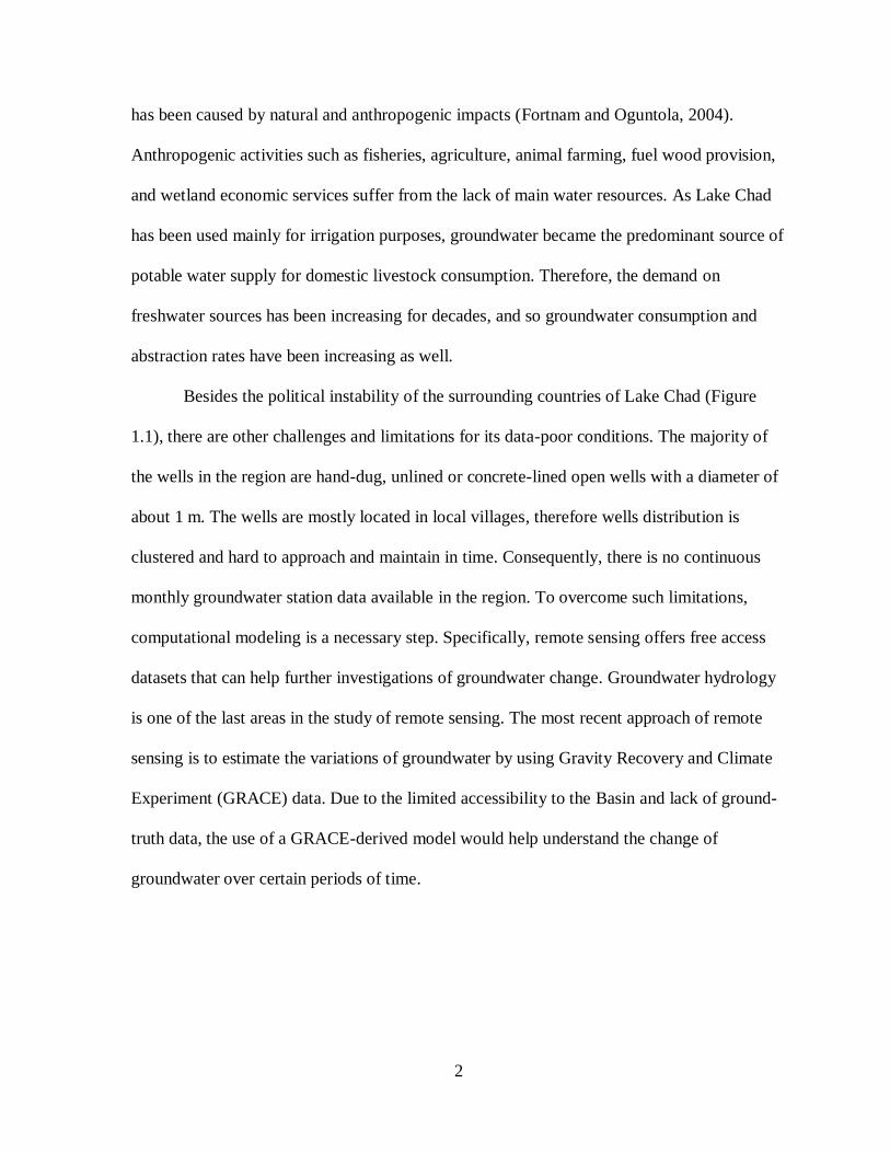
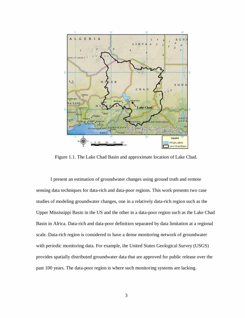
Figure 1.1. The Lake Chad Basin and approximate location of Lake Chad.

I present an estimation of groundwater changes using ground truth and remote

sensing data techniques for data-rich and data-poor regions. This work presents two case

studies of modeling groundwater changes, one in a relatively data-rich region such as the

Upper Mississippi Basin in the US and the other in a data-poor region such as the Lake Chad

Basin in Africa. Data-rich and data-poor definition separated by data limitation at a regional

scale. Data-rich region is considered to have a dense monitoring network of groundwater

with periodic monitoring data. For example, the United States Geological Survey (USGS)

provides spatially distributed groundwater data that are approved for public release over the

past 100 years. The data-poor region is where such monitoring systems are lacking.

Lake Chad

4

In the present study, I compare ground truth and GRACE-based data on the Upper

Mississippi Basin to verify the accuracy of GRACE modeling and understand how modeling

conditions would affect the model accuracy. After finding the most accurate GRACE

modeling setup, I apply the same setup by only using GRACE data to the Ngadda catchment,

a sub-basin of the Lake Chad Basin. My goal is to understand the spatial and temporal

variability of groundwater near the Lake Chad since there is no ground-based monitoring

effort. Consequently, I would be able to answer how the GRACE modeling can help

investigate groundwater at the data poor regions. In addition, I discuss the challenges of

using ground truth and remote sensing data with their advantages and disadvantages.

1.2 GRACE in General.

GRACE is a twin-satellite mission launched by the National Aeronautics and Space

Administration (NASA) and the German Aerospace Center (DLR) in March 17th 2002, to

make detailed measurements of Earth’s gravity field and investigate Earth’s water reservoirs,

over land, ice and oceans. In addition, the mission has several partners for design,

construction and launch, such as Jet Propulsion Laboratory (JPL), the University of Texas

Center for Space Research (CSR), the German Research Centre for Geosciences (GFZ), as

well as Astrium GmBH, Space System Loral (SS/L), Onera and Eurocke GmBH.

The basic concept of GRACE is based on gravity and its proportional relationship

with earth density. Gravity is a force that pulls two masses together, while density is defined

as mass in a given volume. Isaac Newton first discovered the law of gravity, and correlated

gravity and density. If the object is denser, its mass increases, then the exerted gravitational

force increases as well. The Earth’s surface is not uniform as it includes objects with

different density, such as mountains, valleys, oceans, and ice caps. Therefore, the density

5

varies from place to place on the Earth’s surface. Consequently, these variations in density

make slight variations in the gravitational field. As a result, GRACE is the only mission to

detect those changes from space.

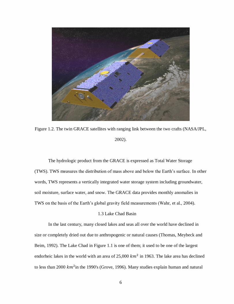
In Figure 1.2, the two satellites stay apart at a distance of about 220 km (137 miles),

and the orbit altitude is about 500 km (311 miles). These satellites spin around the Earth 16

times a day, and produces global coverage every 30 days (a month) from a single source or

position in space. The satellites detect minute variations in the Earth’s surface mass below as

well as variations in the Earth’s gravitational force. When the satellites travel 500 km above

the earth in space, the front satellite captures the area with higher gravity; it is slightly pulled

toward the area with higher density and speeds up. As soon as the front satellite passed over

the area of higher gravity, it slows down, but the trailing satellite speeds up. The distance

between two satellites changes again. As the trailing satellite passes the region of higher

density it slows down as well which does not affect the front satellite in the same time. These

minute expansions and contractions of the distance between satellites are measured using the

microwave K-band ranging instrument, thus are able to map the gravitational field of the

Earth surface. In any one place of the measurement, the data is exactly positioned from

Global Positioning System (GPS) receivers. The main advantage of the GRACE mission is

the high-precision of GPS receiver, which helps precisely map Earth’s gravity field within 1

micron (or the width of a human hair). Consequently, high-resolution maps allow looking at

the Earth’s gravitational field from the large scale to finer-scale over both land and sea.

6

Figure 1.2. The twin GRACE satellites with ranging link between the two crafts (NASA/JPL,

2002).

The hydrologic product from the GRACE is expressed as Total Water Storage

(TWS). TWS measures the distribution of mass above and below the Earth’s surface. In other

words, TWS represents a vertically integrated water storage system including groundwater,

soil moisture, surface water, and snow. The GRACE data provides monthly anomalies in

TWS on the basis of the Earth’s global gravity field measurements (Wahr, et al., 2004).

1.3 Lake Chad Basin

In the last century, many closed lakes and seas all over the world have declined in

size or completely dried out due to anthropogenic or natural causes (Thomas, Meybeck and

Beim, 1992). The Lake Chad in Figure 1.1 is one of them; it used to be one of the largest

endorheic lakes in the world with an area of 25,000 𝑘𝑚2 in 1963. The lake area has declined

to less than 2000 𝑘𝑚2in the 1990's (Grove, 1996). Many studies explain human and natural

7

impacts on the water resources of the Lake Chad, such as: two severe droughts that occurred

in the periods 1972-1974 and 1983-1987 (Kimmage and Adams, 1992); desertification

(Intergovernmental Panel on Climate Change (IPCC), 2001); overgrazing (Food and

Agriculture Organization (FAO), 2009); irrigation activities (Isiorho and Njock-Libii, 1996);

vegetation removal and modification (Keith & Plowers, 1997); deforestation (Neiland and

Verinumbe, 1990); along with population increase (UN Population Division, 2002).

Although the Lake Chad shrinkage has been studied broadly, understanding of groundwater

variations remains poor in the region due to lack of data and challenges to direct access in the

region.

Since Lake Chad is a closed lake, its surface water completely depends on its inflow.

The largest sub-system feeding the lake is the Chari-Logone River system (650,000 𝑘𝑚2

basin area) which supplies 95% of total inflow to the lake (FAO, 2009). The Chari River

flows from the Central African Republic in the south-southeast from the lake, and reaches the

southern pool of the Lake. The second important sub-system is Komadugu-Yobe River

(148,000 𝑘𝑚2 basin area) which flows in from northern Nigeria and Niger. Although the

river contributes only about 2.5% of the total inflow to the Lake, it is the only persistent river

flowing into the northern pool of the Lake.

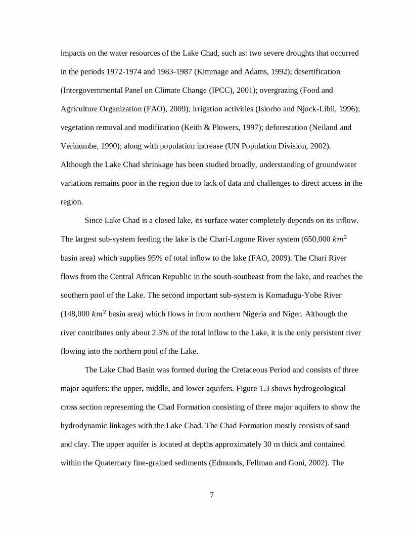
The Lake Chad Basin was formed during the Cretaceous Period and consists of three

major aquifers: the upper, middle, and lower aquifers. Figure 1.3 shows hydrogeological

cross section representing the Chad Formation consisting of three major aquifers to show the

hydrodynamic linkages with the Lake Chad. The Chad Formation mostly consists of sand

and clay. The upper aquifer is located at depths approximately 30 m thick and contained

within the Quaternary fine-grained sediments (Edmunds, Fellman and Goni, 2002). The

8

aquifer is hydrologically connected to the Lake Chad. Groundwater at this aquifer is suitable

mainly for domestic use through wells and boreholes (Odada, Oyebande and Oguntola,

2006). While the upper aquifer is unconfined, the middle aquifer is a confined aquifer

consisting of fine sands and clays between 450 and 620 m depths from the surface (Kindler,

et al. 1990). The water from middle aquifer is mainly used for domestic and livestock use.

Finally, lower aquifer is also a confined aquifer consisting mostly of sand and clayey sand

deposited in the Cretaceous period. The lower aquifer is hardly explored as the approximate

depth to the aquifer is more than 700 meters from the ground surface. The city Maiduguri

heavily drilled boreholes in and around the city for water and gas exploration, which

provides most of the information about the lithology, geometry and hydrogeology of the

aquifers (Bumba, Kida and Bunu, 1985).

Figure 1.3. Hydrogeological cross section of Lake Chad (Source: Schneider, 1991).

9

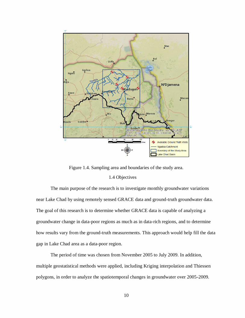
As a case study, the present study focuses on the Ngadda River system (14,400 𝑘𝑚2

catchment area) as shown in Figure 1.4. The area of study is about 48,633 km2. The climate

is semiarid with a long dry season and a short rainy season lasting generally between May

and September. The main city in the area is Maiduguri with a population of 1,197,497 by

2009. The Ngadda River system originates in the Mandara Hills (Northern Cameroon) and

passes through the city of Maiduguri before entering the lake. There is an 80 𝑘𝑚2 swamp

further downstream of the Ngadda Catchment (Nigeria side) which is formed from where the

river does not provide a consistent water supply to the Lake (FAO 1997). However, the

Ngadda River makes a very negligible contribution to the Lake’s inflow in the wet season

since it loses most of its water in a 7 km wide flood plain and swamps in its northwestern

flow. In addition, the system includes the Alau Dam (162 million m3 reservoir), which is

located in the southeast of Maiduguri. After its construction, the Alau reservoir had never

filled to its expected level (Olofin, 1997).

10

Figure 1.4. Sampling area and boundaries of the study area.

1.4 Objectives

The main purpose of the research is to investigate monthly groundwater variations

near Lake Chad by using remotely sensed GRACE data and ground-truth groundwater data.

The goal of this research is to determine whether GRACE data is capable of analyzing a

groundwater change in data-poor regions as much as in data-rich regions, and to determine

how results vary from the ground-truth measurements. This approach would help fill the data

gap in Lake Chad area as a data-poor region.

The period of time was chosen from November 2005 to July 2009. In addition,

multiple geostatistical methods were applied, including Kriging interpolation and Thiessen

polygons, in order to analyze the spatiotemporal changes in groundwater over 2005-2009.

11

In order to assure that GRACE data is applicable to the analysis of groundwater

changes and compare it with ground-truth data, the GRACE modelling was applied to the

Upper Mississippi Basin as an example of a data rich region. After the verification of a

successful modeling approach, the technique was employed to Lake Chad as a data poor

region. The specific objectives of the research are as follows:

To evaluate applicability and accuracy of GRACE satellite data for

monitoring of groundwater in a data-poor region,

To investigate the effects of physical parameters and model parameters in the

GRACE modeling for data rich and data poor regions,

To understand advantages and disadvantages of GRACE modeling for

groundwater monitoring in the Lake Chad Basin as a data poor region.

12

CHAPTER 2

LITERATURE REVIEW

2.1 Groundwater and Remote Sensing Studies for the Lake Chad Basin

Groundwater in the Lake Chad Basin is the predominant source of potable water

supply for domestic livestock consumption while surface water of the Lake Chad is used

mainly for irrigation purposes. Overall, water balance assumes that decrease in rainfall

amount causes decreasing in surface runoff and stream discharge equally well. As a

consequence, groundwater levels have had moderate declines due to a decrease in aquifer

recharge and the increased sinking of boreholes (Fortnam and Oguntola, 2004). Some

specific groundwater reserves decreased due to overexploitation. For instance, Isiorho,

Oguntola and Olojoba (2000) confirmed groundwater drawdowns of several tens of meters in

the Maiduguri area of Nigeria due to groundwater overexploitation. Isiorho et al. (2000)

stated that about 537 wash boreholes were drilled between 1985 and 1989 after droughts of

the 1980s. The quality of the drilling work was unsatisfactory since the contractors did not

use hydro-geological data when locating wells. Additionally, local people leave them

uncapped for their own use. As a result, most of these boreholes are opened and free flowing.

Consequently, this free flow is inefficient and results loss of a great amounts of water with

high evaporation rates in the region (Isiohro, et al., 2000).

On the other hand, some catchment areas showed an increase in runoff and discharge,

and following increase of groundwater. For example, Niger River and the Nakambe River in

the West Africa had increasing discharge and runoff over a severe drought period between

1968 and 1995 (Descroix, et al., 2009). During the same drought period, there was an

increase of groundwater at Niamey in Niger. Albergel (1987) called this phenomena as a

13

‘Sahelian Paradox’ which might happen as a result of deforestation by irrigation, biomass

burning, and soil compaction. Favreau et al. (2002) discovered a rise of groundwater near the

Niger River as a result of increased runoff and recharge through topographic depression

zones. Luxereau, Genthon and Karimou (2012) found out that the discharge was almost

constant in the last five decades at Diffa in the downstream of the Yobe River in spite of a

rainfall decline. Therefore, another assumption is that when runoff increases, discharge into

the River increases as well due to deforestation or cultivation since the 1950s (Mahe’ and

Paturel, 2009; Luxereau, et al., 2012).

The Quaternary aquifer of the Lake Chad has large natural piezometric depressions,

which are found in the southeast of Niger, central Chad, and northeastern Nigeria (Leblanc,

et al., 2007). Schneider (1966) and Lake Chad Basin Commission (LCBC) (1969) first

reported the piezometric depressions, but the origins of the depressions are not yet well

understood. The piezometric depressions might occur due to recharge changes, aquifer

characteristics, land cover and vegetation changes, interactions with surface water, and

overexploitation. Arad and Kafri (1975) made a hypothesis of a perched “hollow” aquifer

existence. They believed that a perched aquifer consists of discontinuous semi-pervious

aquicludes, which provides a form of a hydrological sink with its separation. However, this

theory has not been proved due to lack of subsurface information. The area of the present

study includes one of those depressions named as Bornu piezometric depression. It is

certainly important to understand the behavior of the piezometric depression and the

sensitivity of the aquifer to related climate changes, but the investigation is challenged due to

lack of data.

14

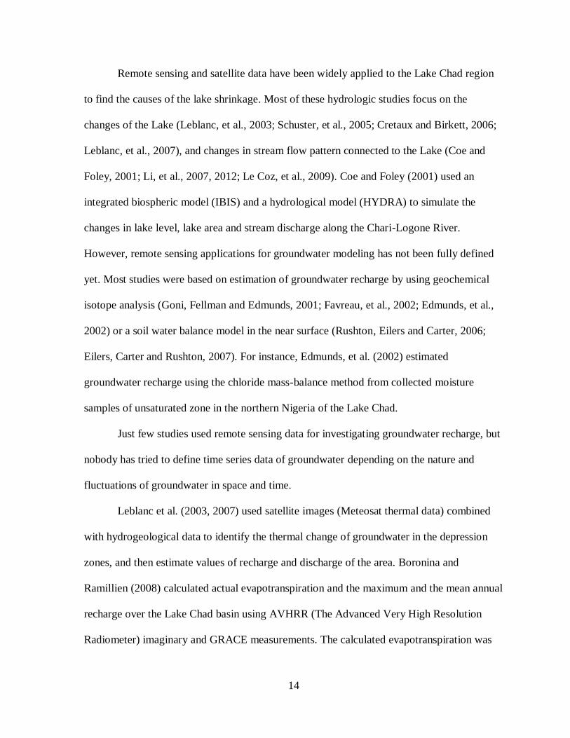
Remote sensing and satellite data have been widely applied to the Lake Chad region

to find the causes of the lake shrinkage. Most of these hydrologic studies focus on the

changes of the Lake (Leblanc, et al., 2003; Schuster, et al., 2005; Cretaux and Birkett, 2006;

Leblanc, et al., 2007), and changes in stream flow pattern connected to the Lake (Coe and

Foley, 2001; Li, et al., 2007, 2012; Le Coz, et al., 2009). Coe and Foley (2001) used an

integrated biospheric model (IBIS) and a hydrological model (HYDRA) to simulate the

changes in lake level, lake area and stream discharge along the Chari-Logone River.

However, remote sensing applications for groundwater modeling has not been fully defined

yet. Most studies were based on estimation of groundwater recharge by using geochemical

isotope analysis (Goni, Fellman and Edmunds, 2001; Favreau, et al., 2002; Edmunds, et al.,

2002) or a soil water balance model in the near surface (Rushton, Eilers and Carter, 2006;

Eilers, Carter and Rushton, 2007). For instance, Edmunds, et al. (2002) estimated

groundwater recharge using the chloride mass-balance method from collected moisture

samples of unsaturated zone in the northern Nigeria of the Lake Chad.

Just few studies used remote sensing data for investigating groundwater recharge, but

nobody has tried to define time series data of groundwater depending on the nature and

fluctuations of groundwater in space and time.

Leblanc et al. (2003, 2007) used satellite images (Meteosat thermal data) combined

with hydrogeological data to identify the thermal change of groundwater in the depression

zones, and then estimate values of recharge and discharge of the area. Boronina and

Ramillien (2008) calculated actual evapotranspiration and the maximum and the mean annual

recharge over the Lake Chad basin using AVHRR (The Advanced Very High Resolution

Radiometer) imaginary and GRACE measurements. The calculated evapotranspiration was

15

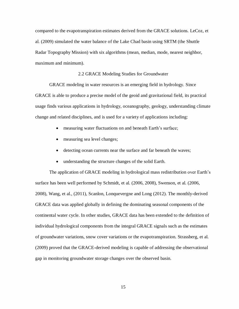
compared to the evapotranspiration estimates derived from the GRACE solutions. LeCoz, et

al. (2009) simulated the water balance of the Lake Chad basin using SRTM (the Shuttle

Radar Topography Mission) with six algorithms (mean, median, mode, nearest neighbor,

maximum and minimum).

2.2 GRACE Modeling Studies for Groundwater

GRACE modeling in water resources is an emerging field in hydrology. Since

GRACE is able to produce a precise model of the geoid and gravitational field, its practical

usage finds various applications in hydrology, oceanography, geology, understanding climate

change and related disciplines, and is used for a variety of applications including:

measuring water fluctuations on and beneath Earth’s surface;

measuring sea level changes;

detecting ocean currents near the surface and far beneath the waves;

understanding the structure changes of the solid Earth.

The application of GRACE modeling in hydrological mass redistribution over Earth’s

surface has been well performed by Schmidt, et al. (2006, 2008), Swenson, et al. (2006,

2008), Wang, et al., (2011), Scanlon, Lonquevergne and Long (2012). The monthly-derived

GRACE data was applied globally in defining the dominating seasonal components of the

continental water cycle. In other studies, GRACE data has been extended to the definition of

individual hydrological components from the integral GRACE signals such as the estimates

of groundwater variations, snow cover variations or the evapotranspiration. Strassberg, et al.

(2009) proved that the GRACE-derived modeling is capable of addressing the observational

gap in monitoring groundwater storage changes over the observed basin.

16

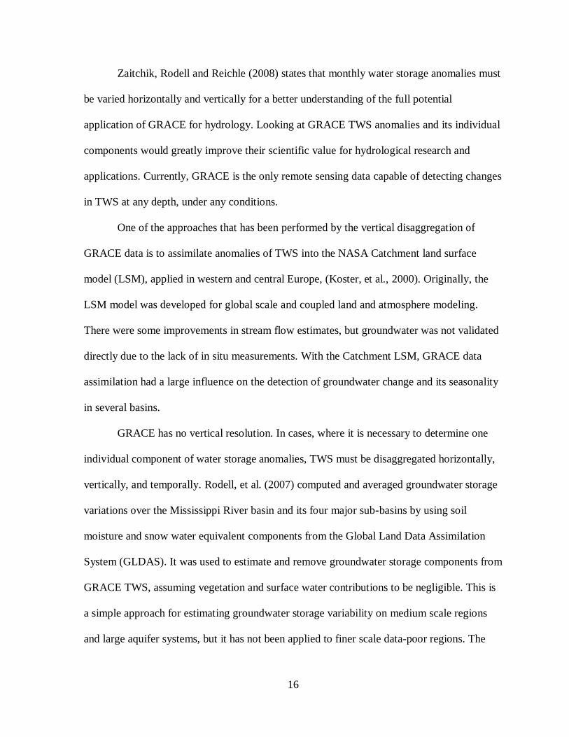
Zaitchik, Rodell and Reichle (2008) states that monthly water storage anomalies must

be varied horizontally and vertically for a better understanding of the full potential

application of GRACE for hydrology. Looking at GRACE TWS anomalies and its individual

components would greatly improve their scientific value for hydrological research and

applications. Currently, GRACE is the only remote sensing data capable of detecting changes

in TWS at any depth, under any conditions.

One of the approaches that has been performed by the vertical disaggregation of

GRACE data is to assimilate anomalies of TWS into the NASA Catchment land surface

model (LSM), applied in western and central Europe, (Koster, et al., 2000). Originally, the

LSM model was developed for global scale and coupled land and atmosphere modeling.

There were some improvements in stream flow estimates, but groundwater was not validated

directly due to the lack of in situ measurements. With the Catchment LSM, GRACE data

assimilation had a large influence on the detection of groundwater change and its seasonality

in several basins.

GRACE has no vertical resolution. In cases, where it is necessary to determine one

individual component of water storage anomalies, TWS must be disaggregated horizontally,

vertically, and temporally. Rodell, et al. (2007) computed and averaged groundwater storage

variations over the Mississippi River basin and its four major sub-basins by using soil

moisture and snow water equivalent components from the Global Land Data Assimilation

System (GLDAS). It was used to estimate and remove groundwater storage components from

GRACE TWS, assuming vegetation and surface water contributions to be negligible. This is

a simple approach for estimating groundwater storage variability on medium scale regions

and large aquifer systems, but it has not been applied to finer scale data-poor regions. The

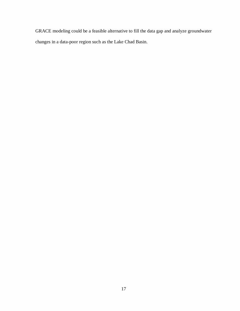
17

GRACE modeling could be a feasible alternative to fill the data gap and analyze groundwater

changes in a data-poor region such as the Lake Chad Basin.

18

CHAPTER 3

METHODOLOGY

3.1 Basic Theory of GRACE

Wolf (1969) presented the first realization of the satellite-to-satellite tracking concept

in the low-low mode. The basics of this concept was to trace the spatio-temporal gravity field

with an increased sensitivity by means of micrometer-precise inter-satellite observation of

two co-planar orbiting satellites. Onboard GPS receivers determine the position of each

spacecraft in a geocentric reference frame, while onboard accelerometers detect the non-

gravitational acceleration. As soon as the residuals infer the gravitational acceleration, the

gravity field is mapped. The desired inter-satellite distance should be smaller than the

altitude; otherwise data will be lost or distorted. Also, since satellites are in such low orbit,

the gravity field determines orders of magnitude more accurately. Relative motion between

satellites is proportional to the integrated differences of the gravity accelerations at its

individual position. The differences are correlated with conservative (gravitational force,

elastic spring force, electric force) and non-conservative forces (tension, air resistance,

normal force).

The dynamic approach for the recovery of global gravity models is based on

Newtonian formulation of the satellites’ equation of motion. Isaak Newton expressed the

interaction force between two masses by the Universal Law of Gravitation:

𝐹 = 𝐺𝑀×𝑚

𝑅2 (1)

where F [N] is the gravitational force,

M and m [kg] are two masses,

R [m] is the distance between two masses,

19

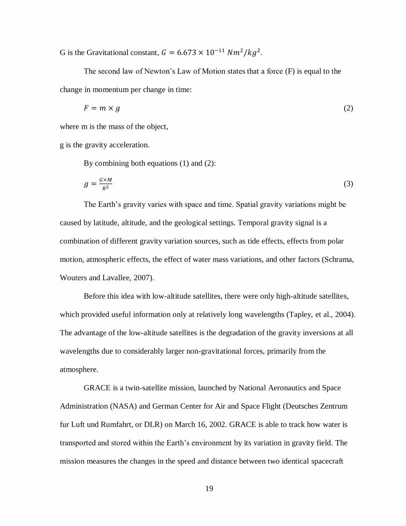
G is the Gravitational constant, 𝐺 = 6.673 × 10−11 𝑁𝑚2/𝑘𝑔2.

The second law of Newton’s Law of Motion states that a force (F) is equal to the

change in momentum per change in time:

𝐹 = 𝑚 × 𝑔 (2)

where m is the mass of the object,

g is the gravity acceleration.

By combining both equations (1) and (2):

𝑔 =𝐺×𝑀

𝑅2 (3)

The Earth’s gravity varies with space and time. Spatial gravity variations might be

caused by latitude, altitude, and the geological settings. Temporal gravity signal is a

combination of different gravity variation sources, such as tide effects, effects from polar

motion, atmospheric effects, the effect of water mass variations, and other factors (Schrama,

Wouters and Lavallee, 2007).

Before this idea with low-altitude satellites, there were only high-altitude satellites,

which provided useful information only at relatively long wavelengths (Tapley, et al., 2004).

The advantage of the low-altitude satellites is the degradation of the gravity inversions at all

wavelengths due to considerably larger non-gravitational forces, primarily from the

atmosphere.

GRACE is a twin-satellite mission, launched by National Aeronautics and Space

Administration (NASA) and German Center for Air and Space Flight (Deutsches Zentrum

fur Luft und Rumfahrt, or DLR) on March 16, 2002. GRACE is able to track how water is

transported and stored within the Earth’s environment by its variation in gravity field. The

mission measures the changes in the speed and distance between two identical spacecraft

20

named GRACE-A and GRACE-B in a polar orbit about 220 kilometers apart and altitude of

500 kilometers.

There are three levels GRACE data produce:

1. Level 1 (Level-1A): the raw data to be calibrated and time-tagged in a non-

destructive sense. Level-1A data products are not distributed to public.

2. Level 2 (Level-1B): the processed products to generate the monthly gravity

field estimates in form of spherical harmonic coefficients.

3. Level 3: the processed data for users who are not familiar with the concept of

spherical harmonics and prefer to access GRACE data products as mass anomalies (Sources:

GRACE Tellus and ICEGM).

The present study adopted the Level 3 data for monthly changes in terrestrial water

storage (TWS) on the basis of the Earth’s global gravity field measurements (Wahr, et al.,

2004). TWS represents a vertically integrated water storage including groundwater, soil

moisture, surface water, snow, and biomass (Strassberg, et al., 2009). To estimate the monthly

groundwater storage variations using GRACE, we adopted a water storage anomalies equation

(Scanlon, et al., 2012):

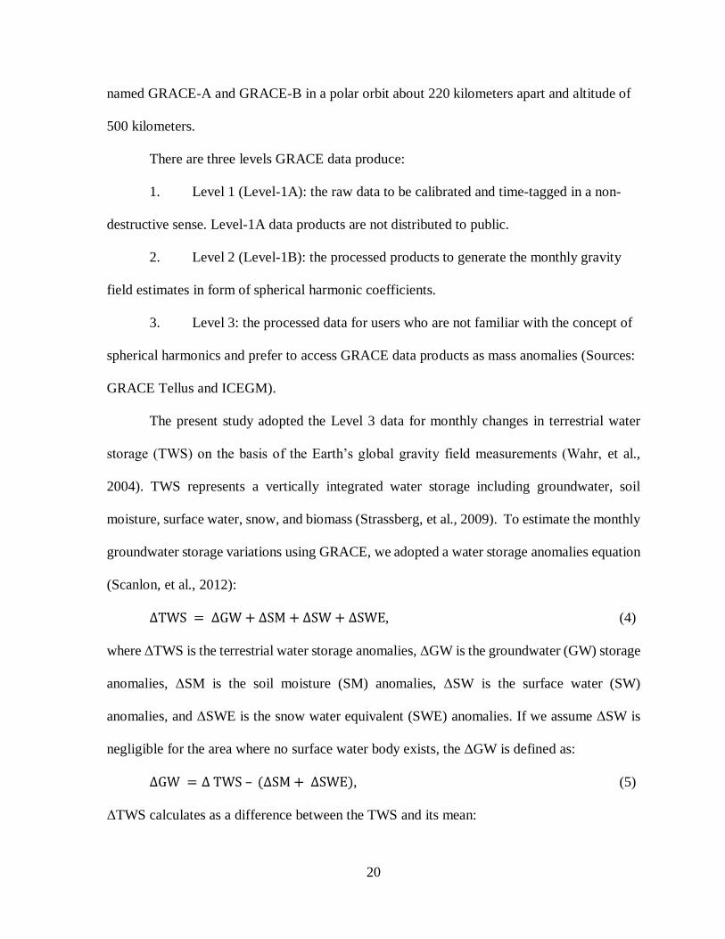
ΔTWS = ΔGW + ΔSM + ΔSW + ΔSWE, (4)

where ΔTWS is the terrestrial water storage anomalies, ΔGW is the groundwater (GW) storage

anomalies, ΔSM is the soil moisture (SM) anomalies, ΔSW is the surface water (SW)

anomalies, and ΔSWE is the snow water equivalent (SWE) anomalies. If we assume ΔSW is

negligible for the area where no surface water body exists, the ΔGW is defined as:

ΔGW = Δ TWS – (ΔSM + ΔSWE), (5)

ΔTWS calculates as a difference between the TWS and its mean:

21

∆𝑇𝑊𝑆𝑖,𝑗,𝑘 = 𝑇𝑊𝑆𝑖,𝑗,𝑘 − ∑ 𝑇𝑊𝑆𝑖,𝑗,𝑘/𝑛𝑛𝑘=1 (6)

Similarily, ΔSM calculates as a difference between the SM and its mean:

∆𝑆𝑀𝑖,𝑗,𝑘 = 𝑆𝑀𝑖,𝑗,𝑘 − ∑ 𝑆𝑀𝑖,𝑗,𝑘/𝑛𝑛𝑘=1 (7)

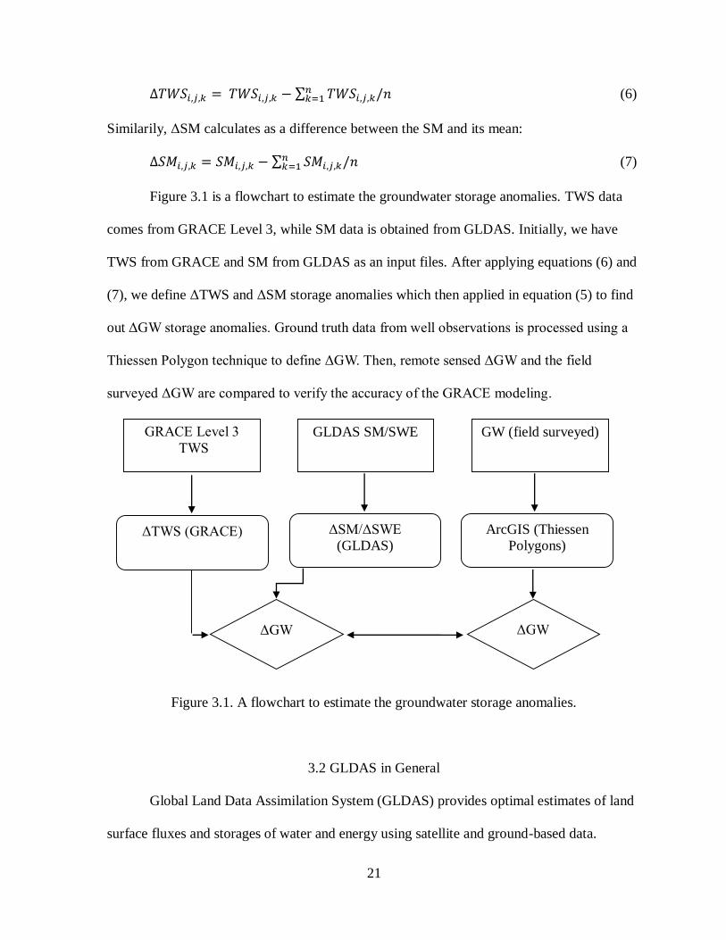
Figure 3.1 is a flowchart to estimate the groundwater storage anomalies. TWS data

comes from GRACE Level 3, while SM data is obtained from GLDAS. Initially, we have

TWS from GRACE and SM from GLDAS as an input files. After applying equations (6) and

(7), we define ΔTWS and ΔSM storage anomalies which then applied in equation (5) to find

out ΔGW storage anomalies. Ground truth data from well observations is processed using a

Thiessen Polygon technique to define ΔGW. Then, remote sensed ΔGW and the field

surveyed ΔGW are compared to verify the accuracy of the GRACE modeling.

Figure 3.1. A flowchart to estimate the groundwater storage anomalies.

3.2 GLDAS in General

Global Land Data Assimilation System (GLDAS) provides optimal estimates of land

surface fluxes and storages of water and energy using satellite and ground-based data.

ΔTWS (GRACE) ΔSM/ΔSWE

(GLDAS)

ArcGIS (Thiessen

Polygons)

GRACE Level 3

TWS

GLDAS SM/SWE GW (field surveyed)

ΔGW

ΔGW

22

GLDAS derives land surface state (soil moisture, surface temperature), and flux

(evaporation, sensible heat flux) parameters. As a land surface component of the hydrological

cycle, soil moisture is the most critical to link the atmospheric and climate processes to the

terrestrial water processes.

GLDAS consists of two versions, GLDAS Version 1 (GLDAS-1) and GLDAS

Version 2 (GLDAS-2). GLDAS-1 includes high quality observational precipitation and solar

radiation input datasets for the period 1979 to present. Specifically, GLDAS-1 is a

combination of NOAA/GDAS fields, NOAA Climate Prediction Center Merged Analysis of

Precipitation (CMAP) (Xie and Arkin, 1997), and the Air Force Weather Agency (AFWA).

In comparison, GLDAS-2 uses reanalyzed meteorological input datasets that have been

corrected using ground-based products for the period 1948-2010. Consequently, GLDAS-2 is

more applicable for a long-term analysis that requires consistency over a long period of time.

In the present study we used GLDAS-1 since we were interested in the recent period, roughly

2002 to present, and the data is updated to within 1-2 months of time.

Currently, GLDAS runs four land surface models (LSMs):

1. The Common Land Model (CLM) is the land model for the Community Earth System

Model (CESM) and Community Atmosphere Model (CAM). It is a collaborative project

between scientists in the Terrestrial Science Section (TSS) and the Climate and Global

Dynamics Division (CGD) at the National Center for Atmospheric Research (NCAR) and the

CESM Land Surface Model (LSM) Working Group. CLM can be run as a stand-alone one-

dimensional model in a coupled and uncoupled to the atmosphere (offline) mode. The soil

model is divided into 10 horizontal layers (Table 1). Thus, CLM model has more dynamic

23

soil moisture with a smaller depth range, which tends to produce higher runoff and lower

evapotranspiration under wet conditions (Zaitchik, Rodell and Olivera, 2010).

2. The National Centers for Environmental Prediction (NCEP)/Oregon State

University/Air Force/Hydrologic Research Lab Model (Noah) was developed by a

collaboration of public and private institutions with the leadership of the NCEP. Like CLM,

Noah is a stand-alone, uncoupled and coupled one-dimensional model. Noah simulates soil

temperature and moisture (both liquid and frozen) for all soil layers (four in this model),

snowpack depth, snowpack water equivalent (one layer model), canopy water content, and

the energy flux and water flux of the surface energy and water balance.

3. The Mosaic model originally was developed for the NASA global climate change.

Like CLM and Noah, Mosaic is a stand-alone, one-dimensional model that can be run both

uncoupled and coupled to the atmospheric models. The model is based on one of the simple

biosphere model with its physics and surface flux calculations. The Mosaic model consists of

three soil layers and a simple one layer snow model.

4. The Variable Infiltration Capacity (VIC) Model was developed, maintained and

upgraded by the University of Washington. Unlike the other three models, VIC is an

uncoupled, calibrated hydrology model, but can be adjusted as a coupled with climate

models. Currently, VIC is running only in a water balance mode, and applied at the

continental and global scales. Therefore, this model is not considered in this study.

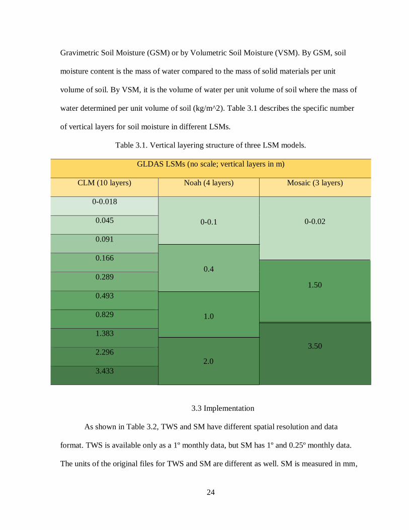
The present study considers only two water balance parameters of GLDAS-1 version:

average layer soil moisture and snow water equivalent from CLM, Noah, and Mosaic LSMs

respectively. The average layer soil moisture is the depth-averaged amount of water in a

specific soil layer beneath the surface. The soil moisture content can be measured by

24

0-0.1

0-0.02

1.50

3.50

0.4

1.0

2.0

Gravimetric Soil Moisture (GSM) or by Volumetric Soil Moisture (VSM). By GSM, soil

moisture content is the mass of water compared to the mass of solid materials per unit

volume of soil. By VSM, it is the volume of water per unit volume of soil where the mass of

water determined per unit volume of soil (kg/m^2). Table 3.1 describes the specific number

of vertical layers for soil moisture in different LSMs.

Table 3.1. Vertical layering structure of three LSM models.

GLDAS LSMs (no scale; vertical layers in m)

CLM (10 layers) Noah (4 layers) Mosaic (3 layers)

0-0.018

0.045

0.091

0.166

0.289

0.493

0.829

1.383

2.296

3.433

3.3 Implementation

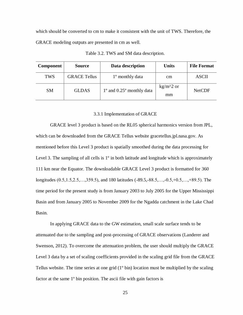
As shown in Table 3.2, TWS and SM have different spatial resolution and data

format. TWS is available only as a 1º monthly data, but SM has 1º and 0.25º monthly data.

The units of the original files for TWS and SM are different as well. SM is measured in mm,

25

which should be converted to cm to make it consistent with the unit of TWS. Therefore, the

GRACE modeling outputs are presented in cm as well.

Table 3.2. TWS and SM data description.

Component Source Data description Units File Format

TWS GRACE Tellus 1º monthly data cm ASCII

SM GLDAS 1º and 0.25º monthly data kg/m^2 or

mm NetCDF

3.3.1 Implementation of GRACE

GRACE level 3 product is based on the RL05 spherical harmonics version from JPL,

which can be downloaded from the GRACE Tellus website gracetellus.jpl.nasa.gov. As

mentioned before this Level 3 product is spatially smoothed during the data processing for

Level 3. The sampling of all cells is 1º in both latitude and longitude which is approximately

111 km near the Equator. The downloadable GRACE Level 3 product is formatted for 360

longitudes (0.5,1.5,2.5,…,359.5), and 180 latitudes (-89.5,-88.5,…,-0.5,+0.5,…,+89.5). The

time period for the present study is from January 2003 to July 2005 for the Upper Mississippi

Basin and from January 2005 to November 2009 for the Ngadda catchment in the Lake Chad

Basin.

In applying GRACE data to the GW estimation, small scale surface tends to be

attenuated due to the sampling and post-processing of GRACE observations (Landerer and

Swenson, 2012). To overcome the attenuation problem, the user should multiply the GRACE

Level 3 data by a set of scaling coefficients provided in the scaling grid file from the GRACE

Tellus website. The time series at one grid (1º bin) location must be multiplied by the scaling

factor at the same 1º bin position. The ascii file with gain factors is

26

CLM4.SCALE_FACTOR.DS.G300KM.asc stored in the ascii directory of GRACE Tellus

website.

After scaling GRACE input data, we created a Python program to estimate the GW

anomalies. The program is coded in Python 2.7 version. The full program code is available in

Appendix A.

Below is a procedure for the GW calculations:

Step 1. Create a separate folder for monthly GRACE data files in a Python directory.

Step 2. Set the boundaries of the study area in GRACE files. One month GRACE file

consists of 1 degree grid resolution file (360 x 180 degrees) for the entire globe. To specify

exact boundaries of the interested area, we need to open GRACE ascii file in ArcGIS and

overlap it with a map of the basin boundaries. Using the ‘Identify’ tool in ArcGIS, we define

the GRACE values over the basin. Then, we open the GRACE file in Microsoft Excel and

define the boundaries of the area by known values. Then, in the program code, we isolate the

rows and columns of the data of interest.

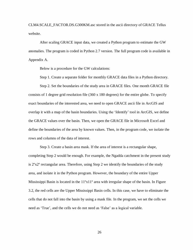
Step 3. Create a basin area mask. If the area of interest is a rectangular shape,

completing Step 2 would be enough. For example, the Ngadda catchment in the present study

is 2ºx2º rectangular area. Therefore, using Step 2 we identify the boundaries of the study

area, and isolate it in the Python program. However, the boundary of the entire Upper

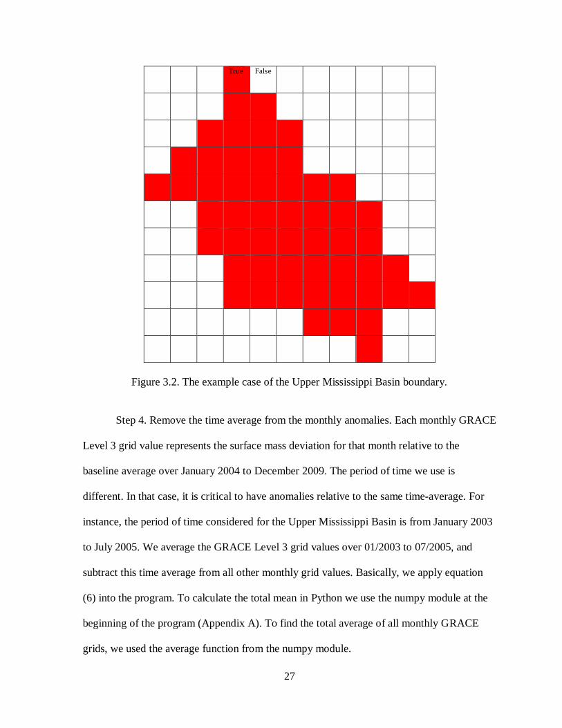
Mississippi Basin is located in the 11ºx11º area with irregular shape of the basin. In Figure

3.2, the red cells are the Upper Mississippi Basin cells. In this case, we have to eliminate the

cells that do not fall into the basin by using a mask file. In the program, we set the cells we

need as ‘True’, and the cells we do not need as ‘False’ as a logical variable.

27

True False

Figure 3.2. The example case of the Upper Mississippi Basin boundary.

Step 4. Remove the time average from the monthly anomalies. Each monthly GRACE

Level 3 grid value represents the surface mass deviation for that month relative to the

baseline average over January 2004 to December 2009. The period of time we use is

different. In that case, it is critical to have anomalies relative to the same time-average. For

instance, the period of time considered for the Upper Mississippi Basin is from January 2003

to July 2005. We average the GRACE Level 3 grid values over 01/2003 to 07/2005, and

subtract this time average from all other monthly grid values. Basically, we apply equation

(6) into the program. To calculate the total mean in Python we use the numpy module at the

beginning of the program (Appendix A). To find the total average of all monthly GRACE

grids, we used the average function from the numpy module.

28

3.3.2 Implementation of GLDAS

GLDAS can be downloaded from the GES GISC website

http://disc.sci.gsfc.nasa.gov/ hydrology/data-holdings. The data was downloaded using

search for data with Mirador database. Mirador is an earth science data search tool developed

at the GES DIS. This database allows selection of the area by latitude and longitude, so we

do not have to download an entire world map as we do in the acquisition of the GRACE data.

All three LSMs with 1º and 0.25º resolution are available on the website. The period of time

is the same as in the GRACE.

The implementation of the GLDAS data into the GW calculations is:

Step 1. Create a separate folder for monthly GLDAS data files in a Python directory.

Step 2. GLDAS data has NetCDF format. NetCDF is a file format for storing

multidimensional scientific data (variables) such as temperature, pressure, wind speed, etc. In

our case, we downloaded NetCDF files with two parameters: soil moisture and snow water

equivalent (for the Upper Mississippi Basin). The NetCDF file can be opened in ArcGIS and

verified the values using the ‘Identify’ tool in ArcGIS. GLDAS data does not require setting

up basin boundaries since this procedure was performed during downloading.

Step 3. Average the GLDAS values over the target period of time, and subtract this

average value from all other monthly grid values. Basically, we apply equation (7) into the

program. If we use all three LSMs, we need to find an average of each model value.

Step 4. Convert GLDAS data from mm to cm by diving by 10.

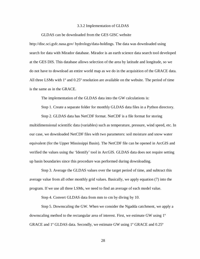
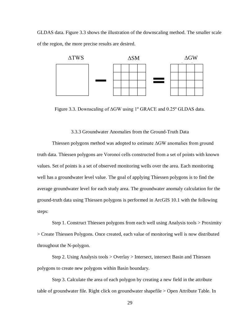
Step 5. Downscaling the GW. When we consider the Ngadda catchment, we apply a

downscaling method to the rectangular area of interest. First, we estimate GW using 1º

GRACE and 1º GLDAS data. Secondly, we estimate GW using 1º GRACE and 0.25º

29

GLDAS data. Figure 3.3 shows the illustration of the downscaling method. The smaller scale

of the region, the more precise results are desired.

Figure 3.3. Downscaling of ΔGW using 1º GRACE and 0.25º GLDAS data.

3.3.3 Groundwater Anomalies from the Ground-Truth Data

Thiessen polygons method was adopted to estimate ΔGW anomalies from ground

truth data. Thiessen polygons are Voronoi cells constructed from a set of points with known

values. Set of points is a set of observed monitoring wells over the area. Each monitoring

well has a groundwater level value. The goal of applying Thiessen polygons is to find the

average groundwater level for each study area. The groundwater anomaly calculation for the

ground-truth data using Thiessen polygons is performed in ArcGIS 10.1 with the following

steps:

Step 1. Construct Thiessen polygons from each well using Analysis tools > Proximity

> Create Thiessen Polygons. Once created, each value of monitoring well is now distributed

throughout the N-polygon.

Step 2. Using Analysis tools > Overlay > Intersect, intersect Basin and Thiessen

polygons to create new polygons within Basin boundary.

Step 3. Calculate the area of each polygon by creating a new field in the attribute

table of groundwater file. Right click on groundwater shapefile > Open Attribute Table. In

ΔTWS ΔSM ΔGW

30

the Table Options select Add Field. In the Add Field window Name the field; Type select

Double > OK. When the new field is added to the attribute table, right click the new field >

Calculate Geometry. Before calculating geometry, verify that the right coordinate system and

display units are chosen.

Step 4. Calculate a percent area for each polygon that represents a portion of the

entire basin. We need to create a new field to calculate this proportion > Field Calculator

from the right click on the new field. The percent area can be defined as:

Percent Area = Intersecting Thiessen Polygon Area / Total Area of a basin.

Step 5. Create a new field and multiply the percent for each Thiessen polygon by

groundwater level value for the polygon it spatially corresponds with. This gives the

weighted groundwater level for each polygon.

Step 6. Sum all the values generated in the previous step to find the weighted average

groundwater level over the basin using Thiessen polygons.

3.4 Statistical Analysis

In this work, trend and linear regression analysis performed to discuss the results. Trend

analysis method of time series data involves comparison of monthly groundwater storage

anomalies from satellite and field measurements over the long period of time to detect general

pattern of a relationship between groundwater storage variables. Linear regression calculates

an equation that minimizes the distance between the fitted line and all of data points. In general,

a model fits the data well if the difference between the observed values and the model’s

predicted values are small and unbiased. Linear regression analysis consists of linear

correlation coefficient and coefficient of determination.

31

The linear correlation coefficient (𝑟) is a measure of the degree of linear relationship

between two variables. The value of 𝑟 varies -1≤ 𝑟 ≤+1. The 𝑟 value of exactly +1 indicates a

perfect positive fit. Positive correlation means that as the value of one variable increases, the

value of the other variable increases, as one decreases the other decreases. The 𝑟 value of

exactly -1 indicates a perfect negative fit. Negative correlation means that as one variable

increases, the other decreases, and vice versa. The value of 𝑟 close to zero means that there is

a random, nonlinear relationship between two variables. A correlation greater than 0.8 is

generally describes as strong, whereas a correlation less than 0.5 is generally described as

weak.

The coefficient of determination or R-squared value (𝑟2) is a statistical measure of how

close the data are to the fitted regression line. If the regression line passes through every point

on the scatter plot, it would be able to explain all of the variation. The farther the line is away

from the points, the less it is able to explain. R-squared value varies 0≤ 𝑟2≤1 or between 0 and

100%, and represents the percent of the data that is the closest to the line of best fit. 0%

indicates that the model explains none of the variability of the response data around its mean.

100% indicates that the model explains all the variability of the response data around its mean.

However, in some applications low R-squared value indicates a good model, or a high R-

squared value indicates a model that does not fit the data well. Therefore, R-squared values

should be always evaluated in conjunction with residual plots and correlation coefficient

where 𝑟 is the square root of 𝑟2.

The Root Mean Square (RMS) deviation is a measure of the difference between values

predicted by a model and the values actually observed from the environment that is being

32

modelled. The difference between values occur due to randomness or inaccurate estimation.

The RMS of a model prediction is defined as the square root of the mean squared error:

𝑅𝑀𝑆 = √∑ (𝑋𝑜𝑏𝑠,𝑖−𝑋𝑚𝑜𝑑𝑒𝑙,𝑖)2𝑛

𝑖=1

𝑛 (8)

where 𝑋𝑜𝑏𝑠 is observed values

𝑋𝑚𝑜𝑑𝑒𝑙 is modelled values at time/place i.

Standard Deviation (STD) provides an understanding of how much variation there is

from mean. In other words, the standard deviation measures how concentrated the data are

around the mean; the more concentrated, the smaller the standard deviation. A large standard

deviation indicated that data values are far from the mean.

33

CHAPTER 4

RESULTS AND DISCUSSION

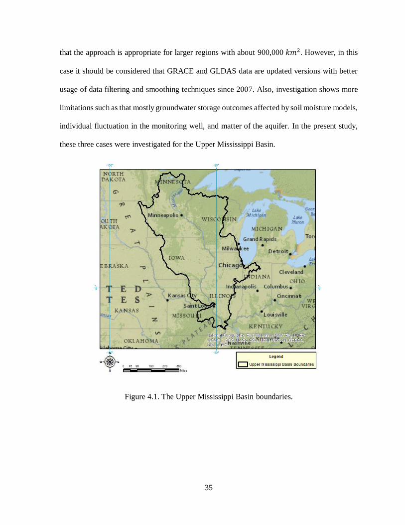
4.1 Data-rich Region: Upper Mississippi Basin

The data-rich region is represented by the Upper Mississippi Basin, one of the four

major sub-basins of the Mississippi River Basin, which stretches from northwest to southeast

of the Upper Midwest of the United States (Figure 4.1). The Upper Mississippi Basin drains

approximately 491,756km2, including a large area of the states of Illinois, Iowa, Minnesota,

Missouri, and Wisconsin. Small portions of Indiana, Michigan, and South Dakota are also

within the basin.

Natural and human factors affect surface and groundwater hydrology over the

Mississippi River Basin as well as its quality, aquatic life in rivers and streams (Stark, et al.,

1999). Besides GRACE satellite-based data, investigation of groundwater changes over the

Upper Mississippi Basin is possible using ground truth data from the USGS Groundwater

Watch Data. The USGS maintains the network of groundwater wells with daily, monthly, or

seasonal observations to monitor the effects of droughts and other climate variability on

groundwater levels. Monitoring groundwater level changes over the Upper Mississippi Basin

is a good case study to find capability of GRACE modeling since there is enough time-series

data. However, many of the groundwater well records have missing daily or monthly values.

To overcome such a limitation, continuous time series for each monitoring station was first

generated using linear interpolation.

Therefore, the methodology of GRACE modeling was applied to the Upper Mississippi

Basin for verification of GRACE efficiency. In the present study, I used a case study of Rodell,

at el. (2007). They estimated groundwater storage anomalies from GRACE water storage data

34

and average GLDAS soil moisture and snow data for the entire Mississippi River Basin

(3,247,804 𝑘𝑚2), and its separate four sub-basins: the Missouri (1,323,998 𝑘𝑚2), Arkansas-

Red-White-Lower Mississippi (903,918 𝑘𝑚2), Ohio-Tennessee (528,132 𝑘𝑚2), and Upper

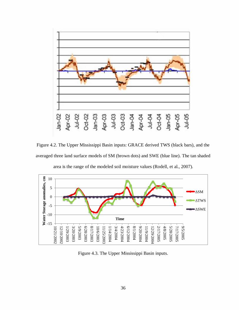
Mississippi (491,756 𝑘𝑚2) using equation (5). Figures 4.2 and 4.3 show the inputs to equation

(5) for the Upper Mississippi Basin from Rodell et al. (2007) and this thesis work. TWS from

GRACE and the average SM and SWE from the three GLDAS land surface models are

anomalies or deviations from the time series mean. The effect of SWE to terrestrial water

storage is almost negligible compared to that of soil moisture.

Then, they evaluated results using groundwater level of 58 well observations in the

unconfined or semi-confined aquifer evenly distributed over the Upper Mississippi basin.

Groundwater levels were converted to regional average groundwater storage variations.

Specific yield estimates were determined over the basin from USGS available metadata and

reports. The Rodell’s work considers specific yield value depending on the sub-basin to be in

the range from 0.02 to 0.32, and its mean of 0.14. I considered specific yield depending only

on the Upper Mississippi Basin as its mean value 0.14. Thiessen polygons were then created

from a set of groundwater levels over the basin to find average groundwater anomalies for each

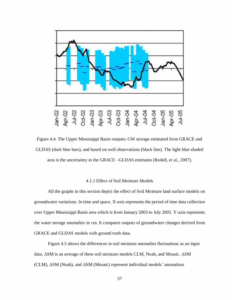
basin. Figure 4.4 represents the groundwater storage estimated from GRACE-GLDAS, and

monitoring well observations. Rodell, et al. (2007) found out that groundwater anomalies

estimates for smaller sub-basins have larger seasonal amplitudes which makes results poorer

in comparison with larger sub-basins since there is little similarity with monitoring well

observation based results. Rodell and Famiglietti (1999) confirmed that the minimum region

area in which GRACE can resolve water mass changes should be no less than 500,000 𝑘𝑚2.

Based on the results for the Mississippi River basin and its four sub-basins, they confirmed

35

that the approach is appropriate for larger regions with about 900,000 𝑘𝑚2. However, in this

case it should be considered that GRACE and GLDAS data are updated versions with better

usage of data filtering and smoothing techniques since 2007. Also, investigation shows more

limitations such as that mostly groundwater storage outcomes affected by soil moisture models,

individual fluctuation in the monitoring well, and matter of the aquifer. In the present study,

these three cases were investigated for the Upper Mississippi Basin.

Figure 4.1. The Upper Mississippi Basin boundaries.

36

Figure 4.2. The Upper Mississippi Basin inputs: GRACE derived TWS (black bars), and the

averaged three land surface models of SM (brown dots) and SWE (blue line). The tan shaded

area is the range of the modeled soil moisture values (Rodell, et al., 2007).

Figure 4.3. The Upper Mississippi Basin inputs.

-15

-10

-5

0

5

10

10

/21

/2002

12

/10

/2002

1/2

9/2

003

3/2

0/2

003

5/9

/20

03

6/2

8/2

003

8/1

7/2

00

3

10

/6/2

00

3

11

/25

/2003

1/1

4/2

004

3/4

/20

04

4/2

3/2

004

6/1

2/2

004

8/1

/20

04

9/2

0/2

004

11

/9/2

004

12

/29

/2004

2/1

7/2

00

5

4/8

/20

05

5/2

8/2

005

7/1

7/2

005

9/5

/20

05

Wate

r S

tora

ge a

nom

ali

es,

cm

Time

ΔSM

ΔTWS

ΔSWE

37

Figure 4.4. The Upper Mississippi Basin outputs: GW storage estimated from GRACE and

GLDAS (dark blue bars), and based on well observations (black line). The light blue shaded

area is the uncertainty in the GRACE –GLDAS estimates (Rodell, et al., 2007).

4.1.1 Effect of Soil Moisture Models

All the graphs in this section depict the effect of Soil Moisture land surface models on

groundwater variations. In time and space, X-axis represents the period of time data collection

over Upper Mississippi Basin area which is from January 2003 to July 2005. Y-axis represents

the water storage anomalies in cm. It compares outputs of groundwater changes derived from

GRACE and GLDAS models with ground truth data.

Figure 4.5 shows the differences in soil moisture anomalies fluctuations as an input

data. ΔSM is an average of three soil moisture models CLM, Noah, and Mosaic. ΔSM

(CLM), ΔSM (Noah), and ΔSM (Mosaic) represent individual models’ anomalous

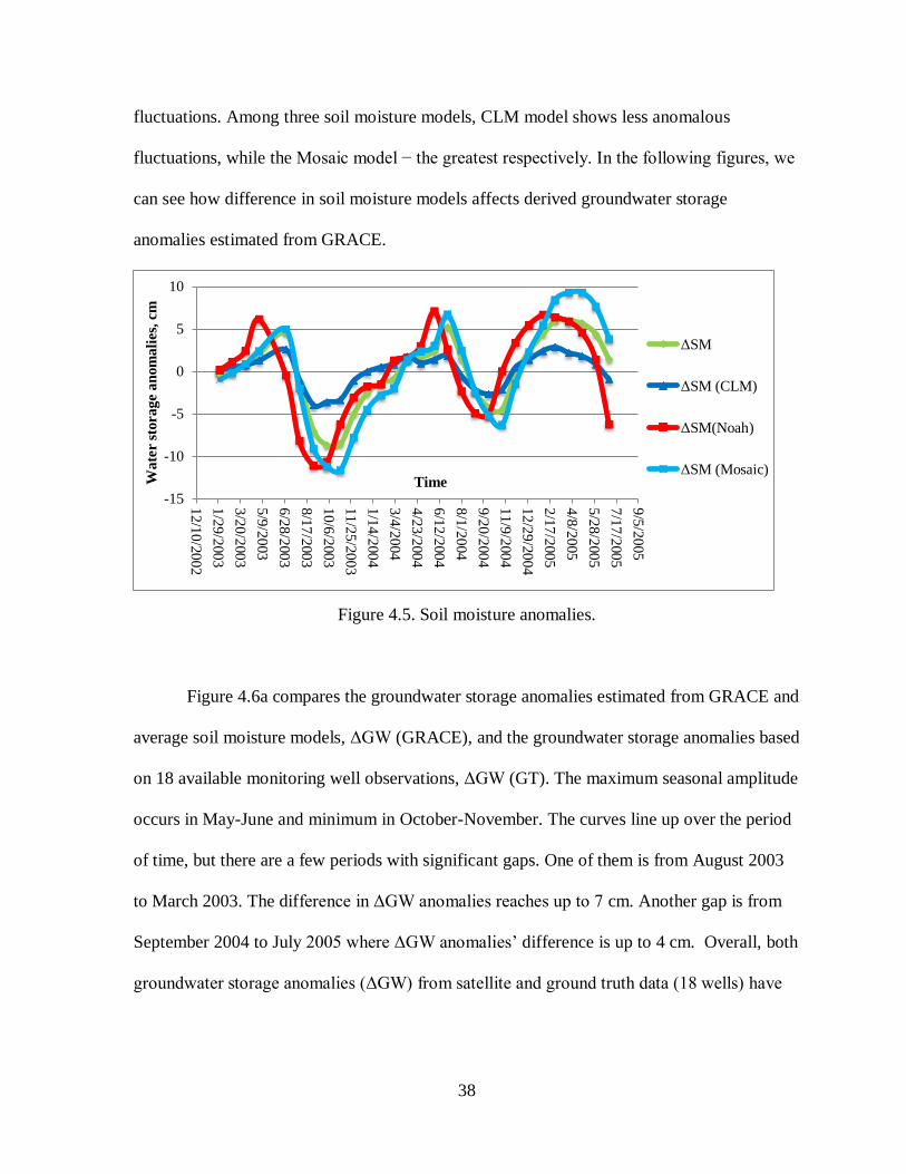
38

fluctuations. Among three soil moisture models, CLM model shows less anomalous

fluctuations, while the Mosaic model − the greatest respectively. In the following figures, we

can see how difference in soil moisture models affects derived groundwater storage

anomalies estimated from GRACE.

Figure 4.5. Soil moisture anomalies.

Figure 4.6a compares the groundwater storage anomalies estimated from GRACE and

average soil moisture models, ΔGW (GRACE), and the groundwater storage anomalies based

on 18 available monitoring well observations, ΔGW (GT). The maximum seasonal amplitude

occurs in May-June and minimum in October-November. The curves line up over the period

of time, but there are a few periods with significant gaps. One of them is from August 2003

to March 2003. The difference in ΔGW anomalies reaches up to 7 cm. Another gap is from

September 2004 to July 2005 where ΔGW anomalies’ difference is up to 4 cm. Overall, both

groundwater storage anomalies (ΔGW) from satellite and ground truth data (18 wells) have

-15

-10

-5

0

5

10

12

/10

/20

02

1/2

9/2

00

3

3/2

0/2

00

3

5/9

/20

03

6/2

8/2

00

3

8/1

7/2

00

3

10

/6/2

00

3

11

/25

/20

03

1/1

4/2

00

4

3/4

/20

04

4/2

3/2

00

4

6/1

2/2

00

4

8/1

/20

04

9/2

0/2

00

4

11

/9/2

00

4

12

/29

/20

04

2/1

7/2

00

5

4/8

/20

05

5/2

8/2

00

5

7/1

7/2

00

5

9/5

/20

05

Wa

ter s

tora

ge a

nom

ali

es,

cm

Time

ΔSM

ΔSM (CLM)

ΔSM(Noah)

ΔSM (Mosaic)

39

increasing trend from January 2003 to July 2005. ΔGW (GRACE) has a positive slope of

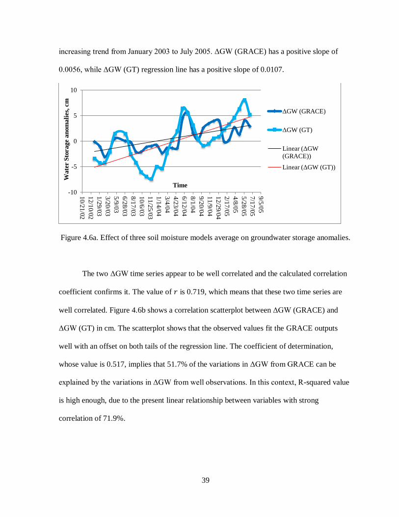
0.0056, while ΔGW (GT) regression line has a positive slope of 0.0107.

Figure 4.6a. Effect of three soil moisture models average on groundwater storage anomalies.

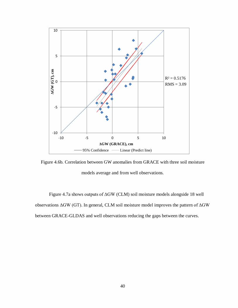
The two ΔGW time series appear to be well correlated and the calculated correlation

coefficient confirms it. The value of 𝑟 is 0.719, which means that these two time series are

well correlated. Figure 4.6b shows a correlation scatterplot between ΔGW (GRACE) and

ΔGW (GT) in cm. The scatterplot shows that the observed values fit the GRACE outputs

well with an offset on both tails of the regression line. The coefficient of determination,

whose value is 0.517, implies that 51.7% of the variations in ΔGW from GRACE can be

explained by the variations in ΔGW from well observations. In this context, R-squared value

is high enough, due to the present linear relationship between variables with strong

correlation of 71.9%.

-10

-5

0

5

10

10

/21

/02

12

/10

/02

1/2

9/0

3

3/2

0/0

3

5/9

/03

6/2

8/0

3

8/1

7/0

3

10

/6/0

3

11

/25

/03

1/1

4/0

4

3/4

/04

4/2

3/0

4

6/1

2/0

4

8/1

/04

9/2

0/0

4

11

/9/0

4

12

/29

/04

2/1

7/0

5

4/8

/05

5/2

8/0

5

7/1

7/0

5

9/5

/05

Wate

r S

tora

ge a

nom

ali

es,

cm

Time

ΔGW (GRACE)

ΔGW (GT)

Linear (ΔGW

(GRACE))

Linear (ΔGW (GT))

40

Figure 4.6b. Correlation between GW anomalies from GRACE with three soil moisture

models average and from well observations.

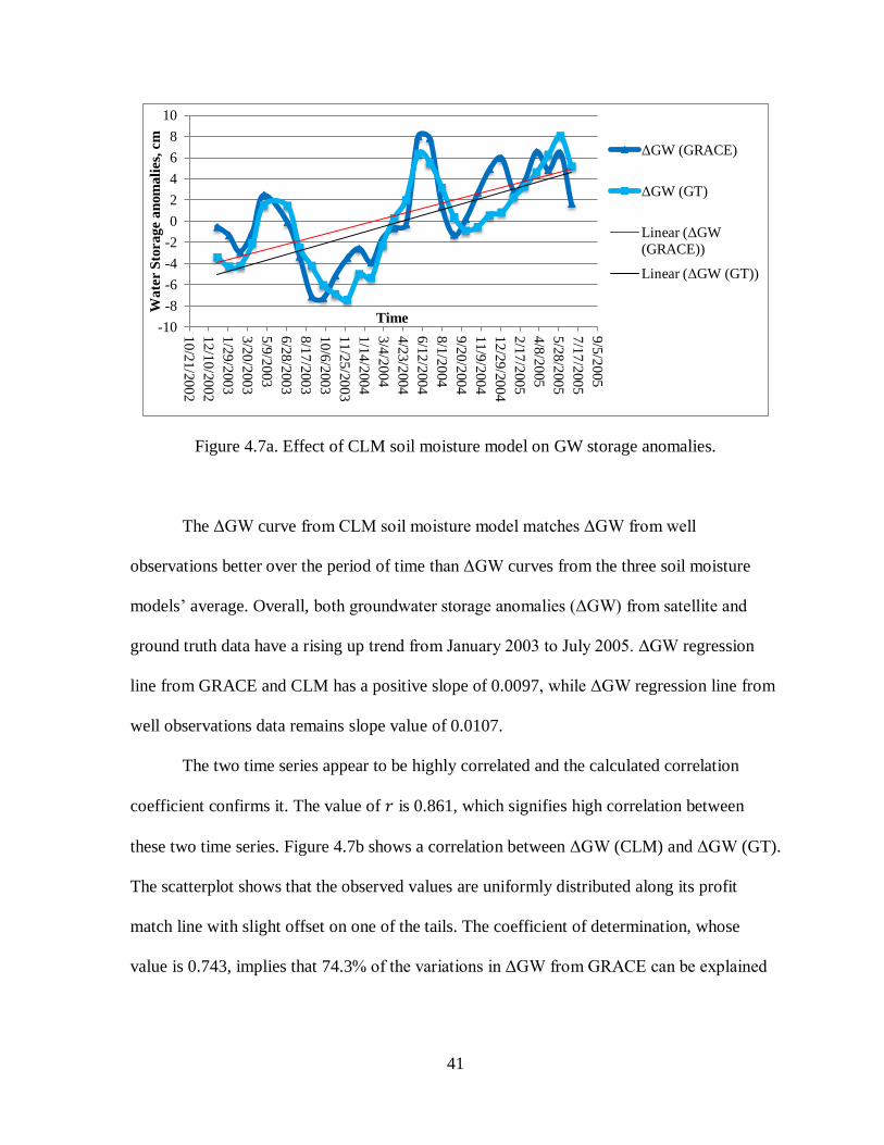
Figure 4.7a shows outputs of ΔGW (CLM) soil moisture models alongside 18 well

observations ΔGW (GT). In general, CLM soil moisture model improves the pattern of ΔGW

between GRACE-GLDAS and well observations reducing the gaps between the curves.

R² = 0.5176

-10

-5

0

5

10

-10 -5 0 5 10

ΔG

W (

GT

), c

m

ΔGW (GRACE), cm

95% Confidence Linear (Predict line)

RMS = 3.09

41

Figure 4.7a. Effect of CLM soil moisture model on GW storage anomalies.

The ΔGW curve from CLM soil moisture model matches ΔGW from well

observations better over the period of time than ΔGW curves from the three soil moisture

models’ average. Overall, both groundwater storage anomalies (ΔGW) from satellite and

ground truth data have a rising up trend from January 2003 to July 2005. ΔGW regression

line from GRACE and CLM has a positive slope of 0.0097, while ΔGW regression line from

well observations data remains slope value of 0.0107.

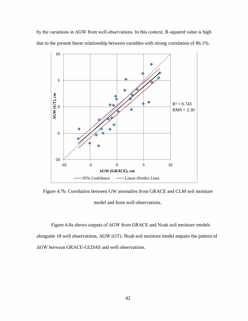
The two time series appear to be highly correlated and the calculated correlation

coefficient confirms it. The value of 𝑟 is 0.861, which signifies high correlation between

these two time series. Figure 4.7b shows a correlation between ΔGW (CLM) and ΔGW (GT).

The scatterplot shows that the observed values are uniformly distributed along its profit

match line with slight offset on one of the tails. The coefficient of determination, whose

value is 0.743, implies that 74.3% of the variations in ΔGW from GRACE can be explained

-10

-8

-6

-4

-2

0

2

4

6

8

10

10/2

1/2

002

12/1

0/2

002

1/2

9/2

003

3/2

0/2

003

5/9

/2003

6/2

8/2

003

8/1

7/2

003

10/6

/2003

11/2

5/2

003

1/1

4/2

004

3/4

/2004

4/2

3/2

004

6/1

2/2

004

8/1

/20

04

9/2

0/2

004

11/9

/2004

12

/29

/20

04

2/1

7/2

005

4/8

/2005

5/2

8/2

005

7/1

7/2

005

9/5

/2005

Wate

r S

torage a

nom

ali

es,

cm

Time

ΔGW (GRACE)

ΔGW (GT)

Linear (ΔGW

(GRACE))

Linear (ΔGW (GT))

42

by the variations in ΔGW from well observations. In this context, R-squared value is high

due to the present linear relationship between variables with strong correlation of 86.1%.

Figure 4.7b. Correlation between GW anomalies from GRACE and CLM soil moisture

model and from well observations.

Figure 4.8a shows outputs of ΔGW from GRACE and Noah soil moisture models

alongside 18 well observations, ΔGW (GT). Noah soil moisture model impairs the pattern of

ΔGW between GRACE-GLDAS and well observations.

R² = 0.743

-10

-5

0

5

10

-10 -5 0 5 10

ΔG

W (

GT

), c

m

ΔGW (GRACE), cm

95% Confidence Linear (Predict Line)

RMS = 2.30

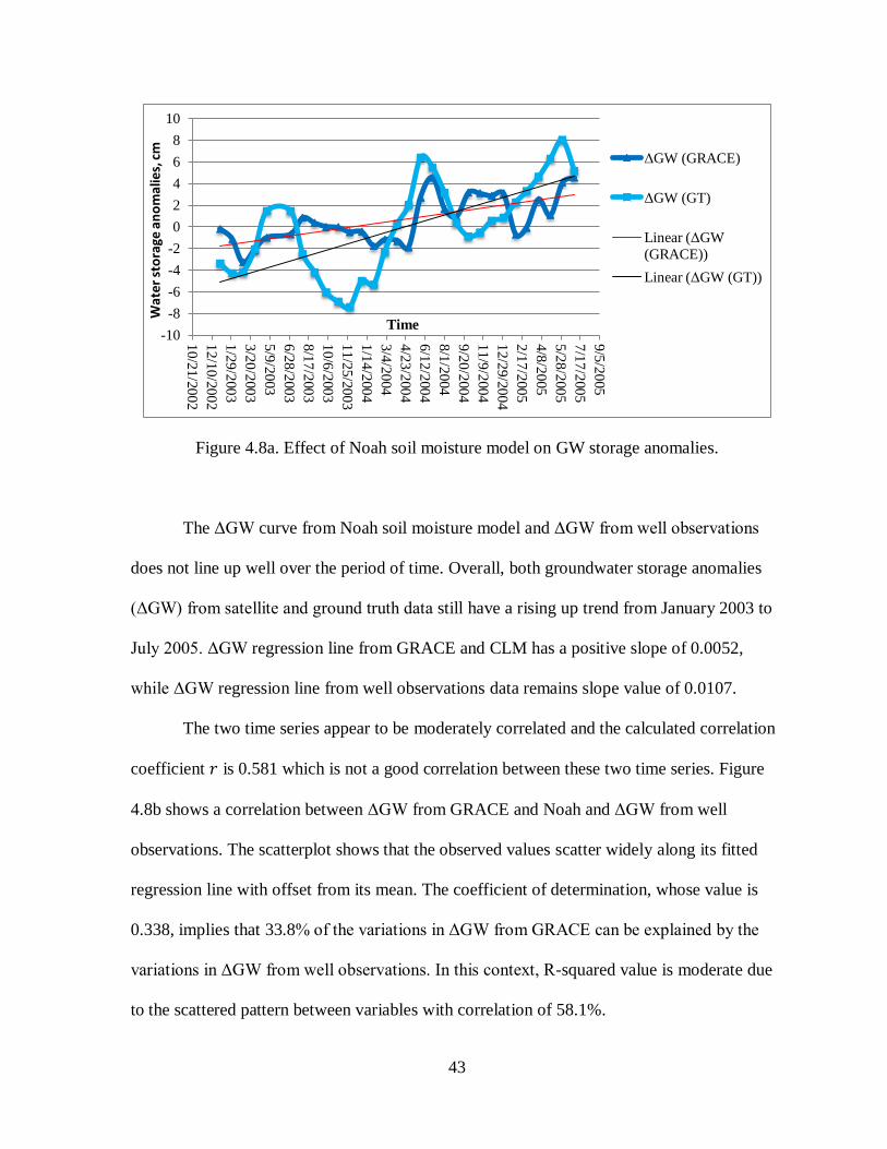
43

Figure 4.8a. Effect of Noah soil moisture model on GW storage anomalies.

The ΔGW curve from Noah soil moisture model and ΔGW from well observations

does not line up well over the period of time. Overall, both groundwater storage anomalies

(ΔGW) from satellite and ground truth data still have a rising up trend from January 2003 to

July 2005. ΔGW regression line from GRACE and CLM has a positive slope of 0.0052,

while ΔGW regression line from well observations data remains slope value of 0.0107.

The two time series appear to be moderately correlated and the calculated correlation

coefficient 𝑟 is 0.581 which is not a good correlation between these two time series. Figure

4.8b shows a correlation between ΔGW from GRACE and Noah and ΔGW from well

observations. The scatterplot shows that the observed values scatter widely along its fitted

regression line with offset from its mean. The coefficient of determination, whose value is

0.338, implies that 33.8% of the variations in ΔGW from GRACE can be explained by the

variations in ΔGW from well observations. In this context, R-squared value is moderate due

to the scattered pattern between variables with correlation of 58.1%.

-10

-8

-6

-4

-2

0

2

4

6

8

10

10/2

1/2

002

12/1

0/2

002

1/2

9/2

003

3/2

0/2

003

5/9

/20

03

6/2

8/2

00

3

8/1

7/2

003

10/6

/2003

11/2

5/2

003

1/1

4/2

004

3/4

/2004

4/2

3/2

004

6/1

2/2

004

8/1

/2004

9/2

0/2

004

11/9

/2004

12

/29

/20

04

2/1

7/2

005

4/8

/2005

5/2

8/2

005

7/1

7/2

005

9/5

/2005

Wat

er s

tora

ge a

no

mal

ies,

cm

Time

ΔGW (GRACE)

ΔGW (GT)

Linear (ΔGW

(GRACE))

Linear (ΔGW (GT))

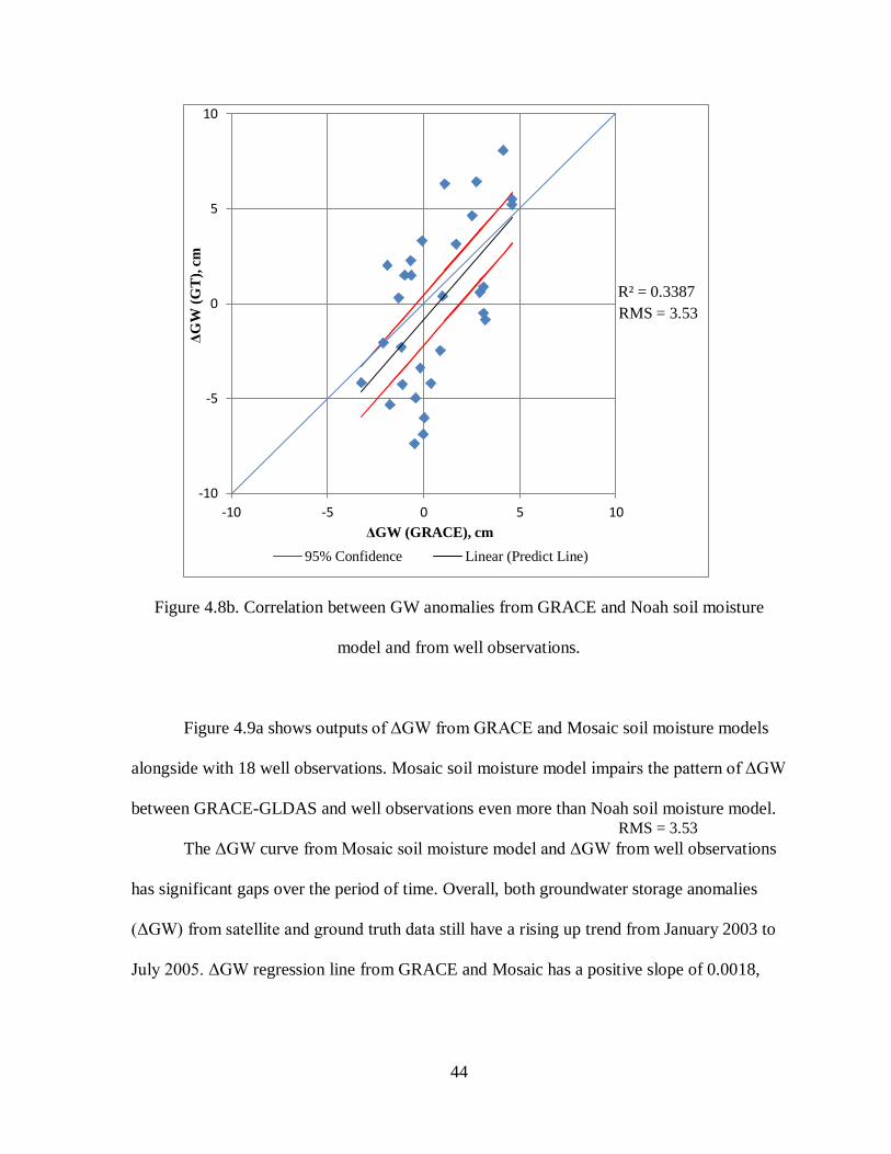
44

Figure 4.8b. Correlation between GW anomalies from GRACE and Noah soil moisture


Figure 4.9a shows outputs of ΔGW from GRACE and Mosaic soil moisture models

alongside with 18 well observations. Mosaic soil moisture model impairs the pattern of ΔGW

between GRACE-GLDAS and well observations even more than Noah soil moisture model.

The ΔGW curve from Mosaic soil moisture model and ΔGW from well observations

has significant gaps over the period of time. Overall, both groundwater storage anomalies

(ΔGW) from satellite and ground truth data still have a rising up trend from January 2003 to

July 2005. ΔGW regression line from GRACE and Mosaic has a positive slope of 0.0018,

R² = 0.3387

-10

-5

0

5

10

-10 -5 0 5 10

ΔG

W (

GT

), c

m

ΔGW (GRACE), cm


RMS = 3.53

RMS = 3.53

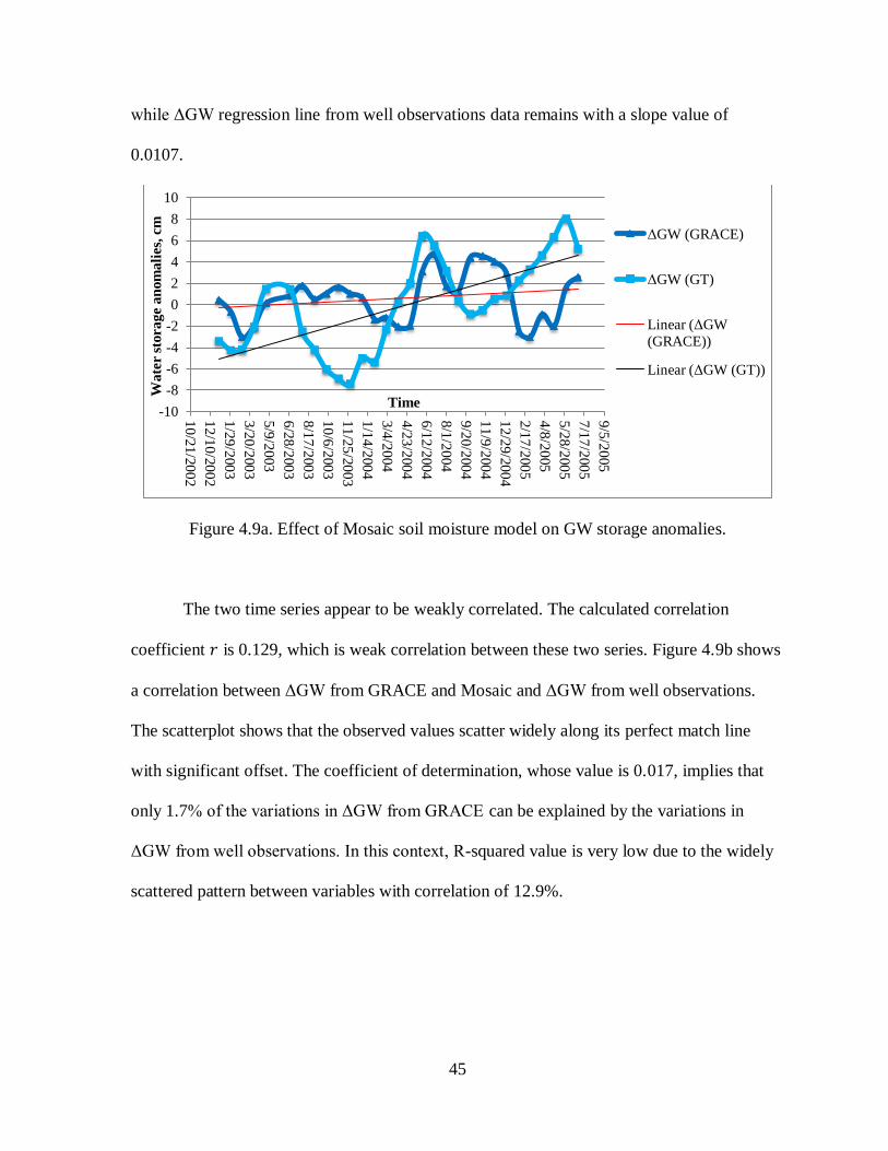
45

while ΔGW regression line from well observations data remains with a slope value of

0.0107.

Figure 4.9a. Effect of Mosaic soil moisture model on GW storage anomalies.

The two time series appear to be weakly correlated. The calculated correlation

coefficient 𝑟 is 0.129, which is weak correlation between these two series. Figure 4.9b shows

a correlation between ΔGW from GRACE and Mosaic and ΔGW from well observations.

The scatterplot shows that the observed values scatter widely along its perfect match line

with significant offset. The coefficient of determination, whose value is 0.017, implies that

only 1.7% of the variations in ΔGW from GRACE can be explained by the variations in

ΔGW from well observations. In this context, R-squared value is very low due to the widely

scattered pattern between variables with correlation of 12.9%.

-10

-8

-6

-4

-2

0

2

4

6

8

10

10

/21

/20

02

12

/10

/20

02

1/2

9/2

00

3

3/2

0/2

00

3

5/9

/20

03

6/2

8/2

00

3

8/1

7/2

00

3

10

/6/2

00

3

11

/25

/20

03

1/1

4/2

00

4

3/4

/20

04

4/2

3/2

00

4

6/1

2/2

00

4

8/1

/20

04

9/2

0/2

00

4

11

/9/2

00

4

12

/29

/20

04

2/1

7/2

00

5

4/8

/20

05

5/2

8/2

00

5

7/1

7/2

00

5

9/5

/20

05

Wate

r s

torage a

nom

ali

es,

cm

Time

ΔGW (GRACE)

ΔGW (GT)

Linear (ΔGW

(GRACE))

Linear (ΔGW (GT))

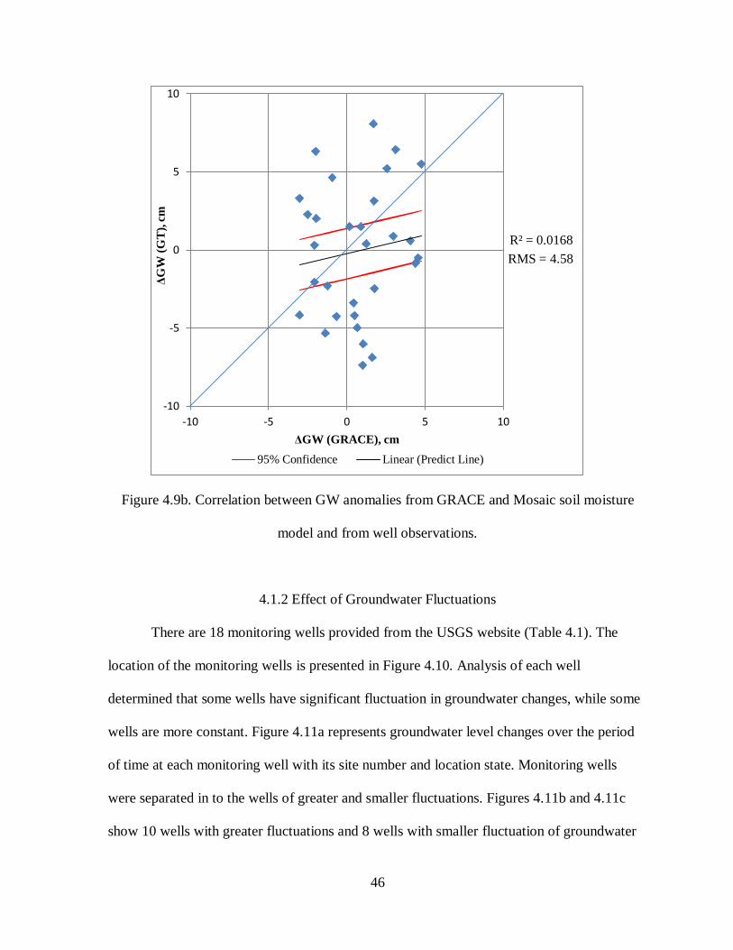
46

Figure 4.9b. Correlation between GW anomalies from GRACE and Mosaic soil moisture


4.1.2 Effect of Groundwater Fluctuations

There are 18 monitoring wells provided from the USGS website (Table 4.1). The

location of the monitoring wells is presented in Figure 4.10. Analysis of each well

determined that some wells have significant fluctuation in groundwater changes, while some

wells are more constant. Figure 4.11a represents groundwater level changes over the period

of time at each monitoring well with its site number and location state. Monitoring wells

were separated in to the wells of greater and smaller fluctuations. Figures 4.11b and 4.11c

show 10 wells with greater fluctuations and 8 wells with smaller fluctuation of groundwater

R² = 0.0168

-10

-5

0

5

10

-10 -5 0 5 10

ΔG

W (

GT

), c

m

ΔGW (GRACE), cm


RMS = 4.58

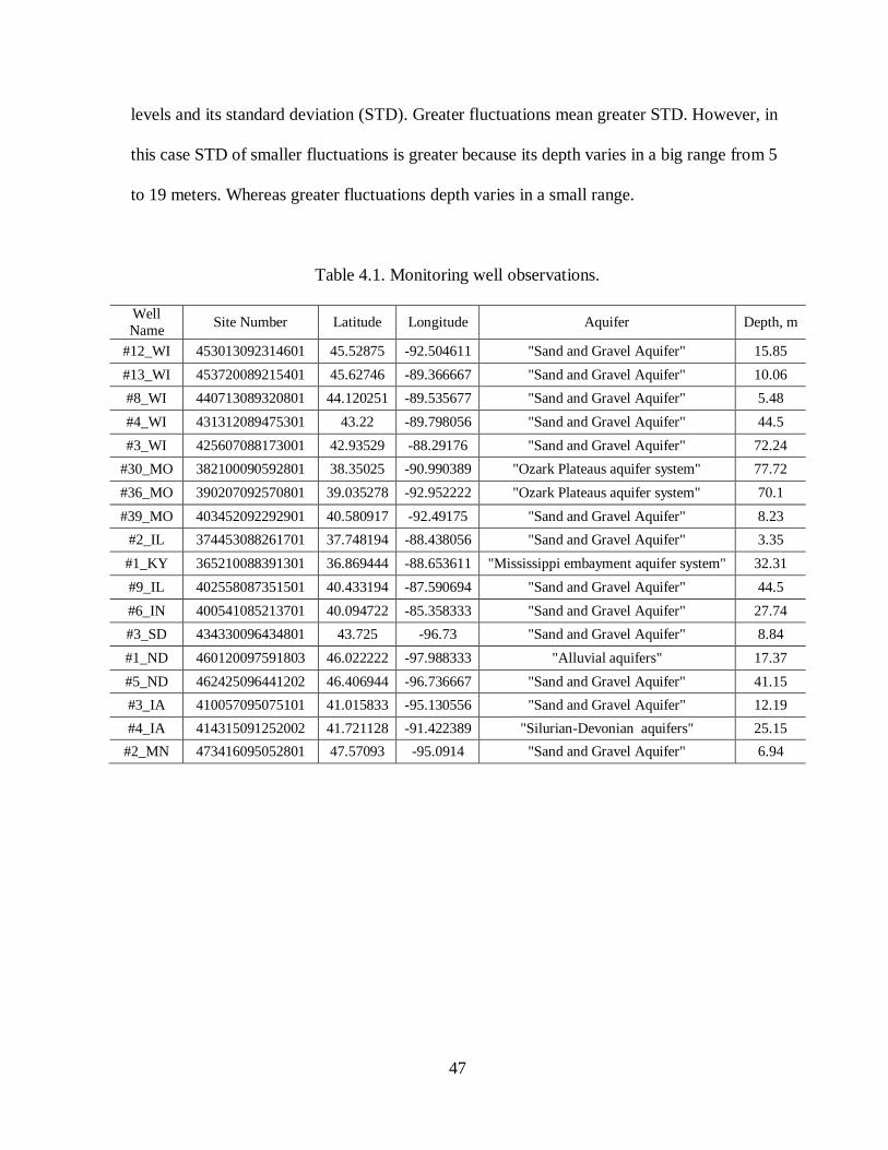
47

levels and its standard deviation (STD). Greater fluctuations mean greater STD. However, in

this case STD of smaller fluctuations is greater because its depth varies in a big range from 5

to 19 meters. Whereas greater fluctuations depth varies in a small range.

Table 4.1. Monitoring well observations.

Well

Name Site Number Latitude Longitude Aquifer Depth, m

#12_WI 453013092314601 45.52875 -92.504611 "Sand and Gravel Aquifer" 15.85





#30_MO 382100090592801 38.35025 -90.990389 "Ozark Plateaus aquifer system" 77.72

#36_MO 390207092570801 39.035278 -92.952222 "Ozark Plateaus aquifer system" 70.1

#39_MO 403452092292901 40.580917 -92.49175 "Sand and Gravel Aquifer" 8.23

#2_IL 374453088261701 37.748194 -88.438056 "Sand and Gravel Aquifer" 3.35

#1_KY 365210088391301 36.869444 -88.653611 "Mississippi embayment aquifer system" 32.31

#9_IL 402558087351501 40.433194 -87.590694 "Sand and Gravel Aquifer" 44.5

#6_IN 400541085213701 40.094722 -85.358333 "Sand and Gravel Aquifer" 27.74

#3_SD 434330096434801 43.725 -96.73 "Sand and Gravel Aquifer" 8.84

#1_ND 460120097591803 46.022222 -97.988333 "Alluvial aquifers" 17.37

#5_ND 462425096441202 46.406944 -96.736667 "Sand and Gravel Aquifer" 41.15

#3_IA 410057095075101 41.015833 -95.130556 "Sand and Gravel Aquifer" 12.19

#4_IA 414315091252002 41.721128 -91.422389 "Silurian-Devonian aquifers" 25.15

#2_MN 473416095052801 47.57093 -95.0914 "Sand and Gravel Aquifer" 6.94

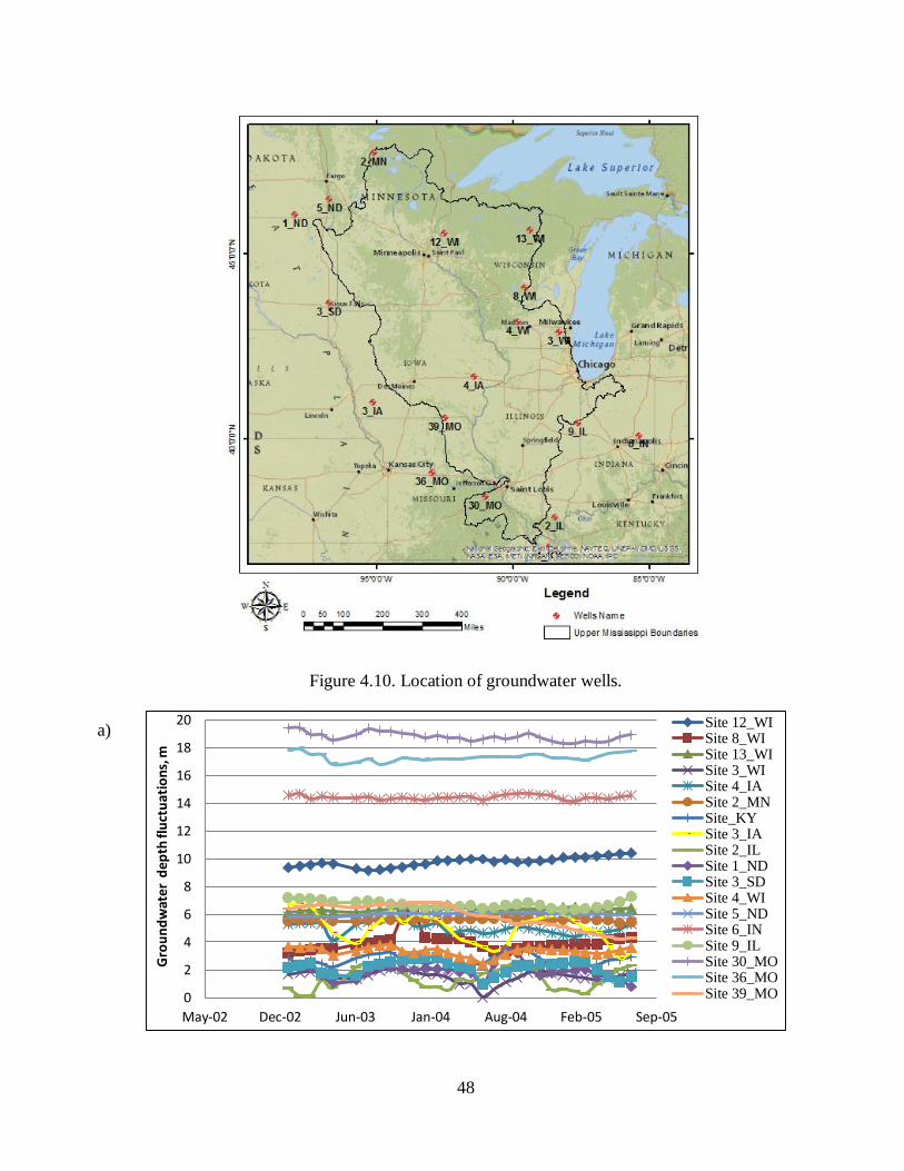
48

Figure 4.10. Location of groundwater wells.

0

2

4

6

8

10

12

14

16

18

20

May-02 Dec-02 Jun-03 Jan-04 Aug-04 Feb-05 Sep-05

Gro

un

dw

ater

dep

th fl

uct

uat

ion

s, m

Site 12_WISite 8_WISite 13_WISite 3_WISite 4_IASite 2_MNSite_KYSite 3_IASite 2_ILSite 1_NDSite 3_SDSite 4_WISite 5_NDSite 6_INSite 9_ILSite 30_MOSite 36_MOSite 39_MO

a)

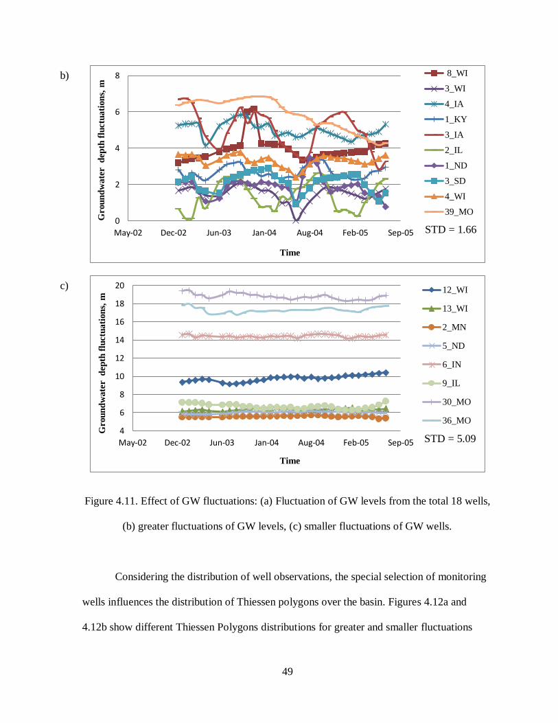
49

Figure 4.11. Effect of GW fluctuations: (a) Fluctuation of GW levels from the total 18 wells,

(b) greater fluctuations of GW levels, (c) smaller fluctuations of GW wells.

Considering the distribution of well observations, the special selection of monitoring

wells influences the distribution of Thiessen polygons over the basin. Figures 4.12a and

4.12b show different Thiessen Polygons distributions for greater and smaller fluctuations

0

2

4

6

8


Grou

nd

wate

r d

ep

th f

luctu

ati

on

s, m

Time

8_WI

3_WI

4_IA

1_KY

3_IA

2_IL

1_ND

3_SD

4_WI

39_MO

4

6

8

10

12

14

16

18

20


Grou

nd

wa

ter d

ep

th f

luctu

ati

on

s, m

Time

12_WI

13_WI

2_MN

5_ND

6_IN

9_IL

30_MO

36_MO

b)

c)

STD = 1.66

STD = 5.09

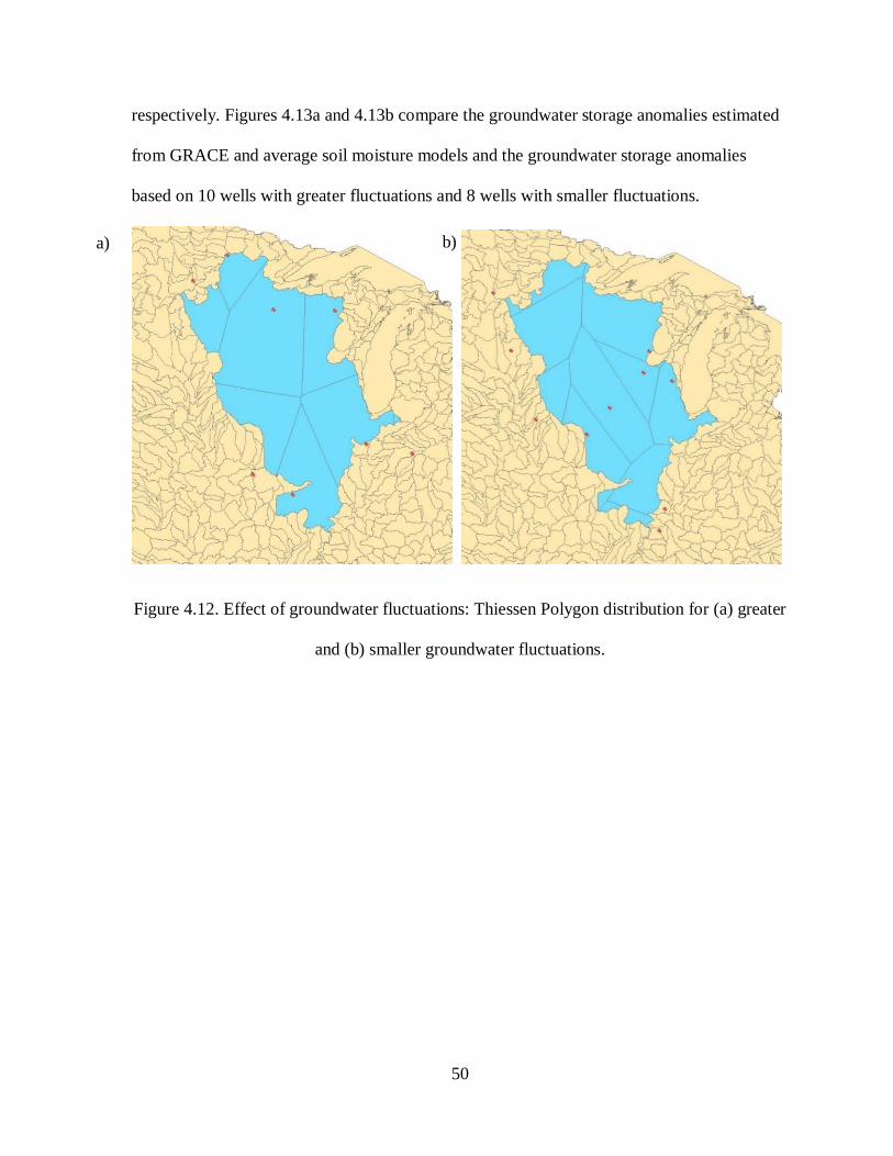
50

respectively. Figures 4.13a and 4.13b compare the groundwater storage anomalies estimated

from GRACE and average soil moisture models and the groundwater storage anomalies

based on 10 wells with greater fluctuations and 8 wells with smaller fluctuations.

Figure 4.12. Effect of groundwater fluctuations: Thiessen Polygon distribution for (a) greater

and (b) smaller groundwater fluctuations.

b) a)

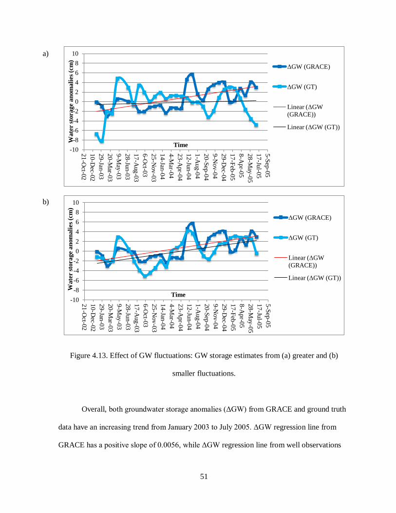
51

Figure 4.13. Effect of GW fluctuations: GW storage estimates from (a) greater and (b)

smaller fluctuations.

Overall, both groundwater storage anomalies (ΔGW) from GRACE and ground truth

data have an increasing trend from January 2003 to July 2005. ΔGW regression line from

GRACE has a positive slope of 0.0056, while ΔGW regression line from well observations

-10

-8

-6

-4

-2

0

2

4

6

8

10

21

-Oct-0

2

10-D

ec-02

29-Jan

-03

20-M

ar-03

9-M

ay-0

3

28

-Jun-0

3

17-A

ug-0

3

6-O

ct-03

25-N

ov-0

3

14-Jan

-04

4-M

ar-04

23-A

pr-0

4

12-Ju

n-0

4

1-A

ug-0

4

20

-Sep

-04

9-N

ov-0

4

29-D

ec-04

17-F

eb-0

5

8-A

pr-0

5

28-M

ay-0

5

17-Ju

l-05

5-S

ep-0

5

Wate

r s

torage a

nom

ali

es

(cm

)

Time

ΔGW (GRACE)

ΔGW (GT)

Linear (ΔGW

(GRACE))

Linear (ΔGW (GT))

-10

-8

-6

-4

-2

0

2

4

6

8

10

21

-Oct-0

2

10

-Dec-0

2

29

-Jan-0

3

20

-Mar-0

3

9-M

ay-0

3

28

-Jun-0

3

17

-Aug

-03

6-O

ct-03

25

-Nov

-03

14

-Jan-0

4

4-M

ar-04

23

-Apr-0

4

12

-Jun-0

4

1-A

ug-0

4

20

-Sep

-04

9-N

ov-0

4

29

-Dec-0

4

17

-Feb

-05

8-A

pr-0

5

28

-May

-05

17

-Jul-0

5

5-S

ep-0

5

Wa

ter s

tora

ge a

nom

ali

es

(cm

)

Time

ΔGW (GRACE)

ΔGW (GT)

Linear (ΔGW

(GRACE))

Linear (ΔGW (GT))

a)

b)

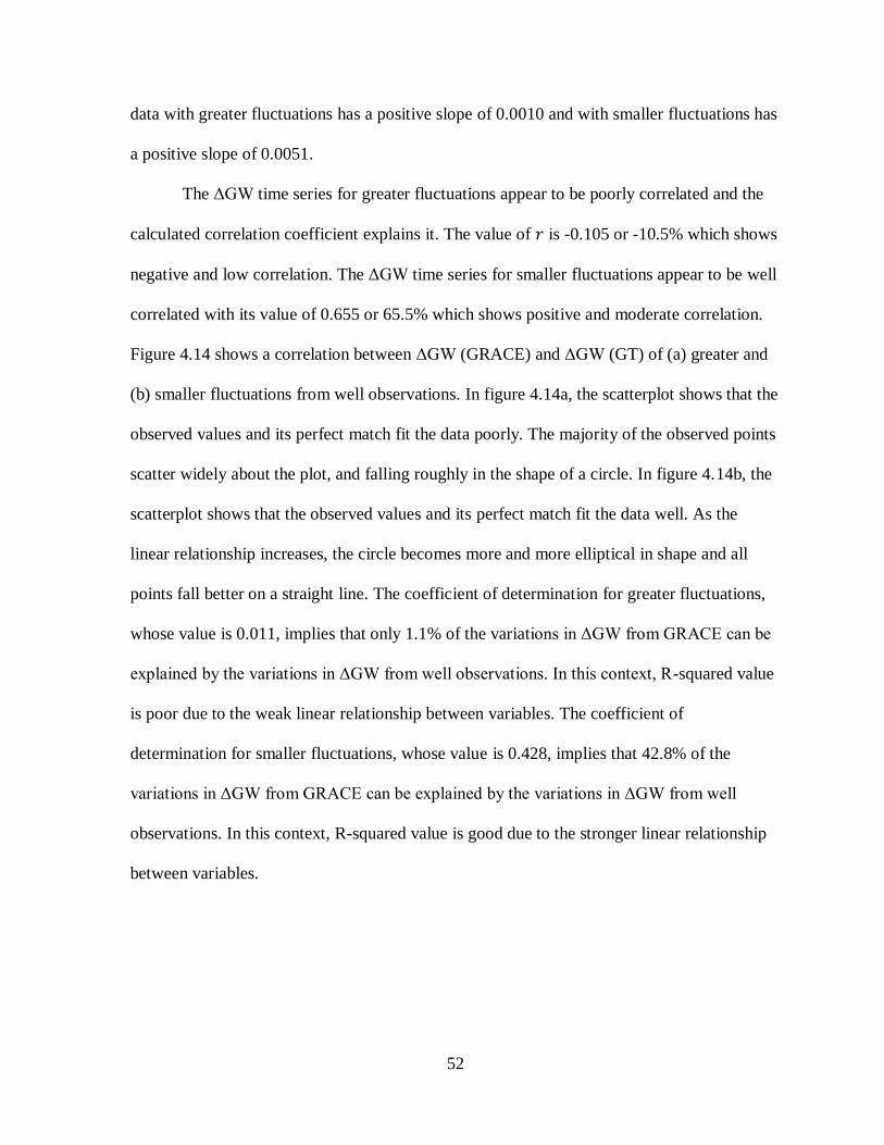
52

data with greater fluctuations has a positive slope of 0.0010 and with smaller fluctuations has

a positive slope of 0.0051.

The ΔGW time series for greater fluctuations appear to be poorly correlated and the

calculated correlation coefficient explains it. The value of 𝑟 is -0.105 or -10.5% which shows

negative and low correlation. The ΔGW time series for smaller fluctuations appear to be well

correlated with its value of 0.655 or 65.5% which shows positive and moderate correlation.

Figure 4.14 shows a correlation between ΔGW (GRACE) and ΔGW (GT) of (a) greater and

(b) smaller fluctuations from well observations. In figure 4.14a, the scatterplot shows that the

observed values and its perfect match fit the data poorly. The majority of the observed points

scatter widely about the plot, and falling roughly in the shape of a circle. In figure 4.14b, the

scatterplot shows that the observed values and its perfect match fit the data well. As the

linear relationship increases, the circle becomes more and more elliptical in shape and all

points fall better on a straight line. The coefficient of determination for greater fluctuations,

whose value is 0.011, implies that only 1.1% of the variations in ΔGW from GRACE can be

explained by the variations in ΔGW from well observations. In this context, R-squared value

is poor due to the weak linear relationship between variables. The coefficient of

determination for smaller fluctuations, whose value is 0.428, implies that 42.8% of the

variations in ΔGW from GRACE can be explained by the variations in ΔGW from well

observations. In this context, R-squared value is good due to the stronger linear relationship

between variables.

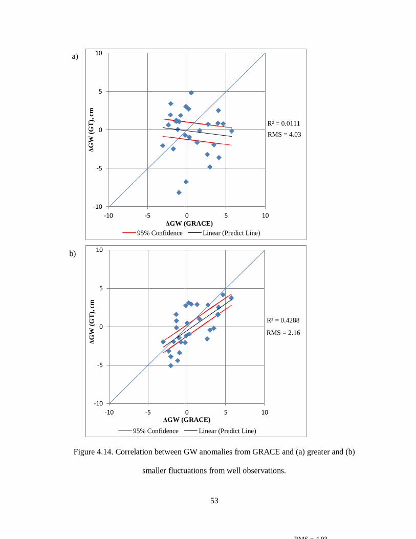
53

Figure 4.14. Correlation between GW anomalies from GRACE and (a) greater and (b)

smaller fluctuations from well observations.

R² = 0.0111

-10

-5

0

5

10

-10 -5 0 5 10

ΔG

W (

GT

), c

m

ΔGW (GRACE)


RMS = 4.03

R² = 0.4288

-10

-5

0

5

10

-10 -5 0 5 10

ΔG

W (

GT

), c

m

ΔGW (GRACE)


RMS = 2.16

a)

b)

RMS = 4.03

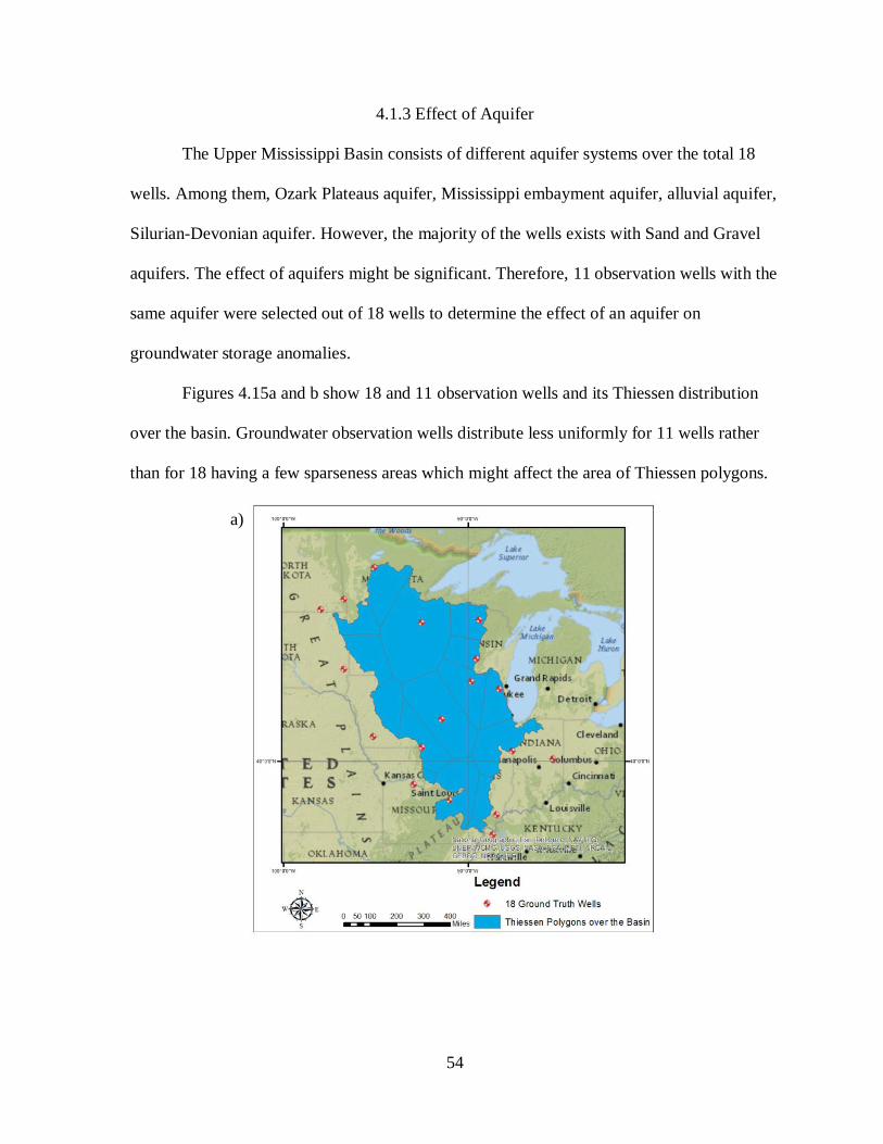
54

4.1.3 Effect of Aquifer

The Upper Mississippi Basin consists of different aquifer systems over the total 18

wells. Among them, Ozark Plateaus aquifer, Mississippi embayment aquifer, alluvial aquifer,

Silurian-Devonian aquifer. However, the majority of the wells exists with Sand and Gravel

aquifers. The effect of aquifers might be significant. Therefore, 11 observation wells with the

same aquifer were selected out of 18 wells to determine the effect of an aquifer on

groundwater storage anomalies.

Figures 4.15a and b show 18 and 11 observation wells and its Thiessen distribution

over the basin. Groundwater observation wells distribute less uniformly for 11 wells rather

than for 18 having a few sparseness areas which might affect the area of Thiessen polygons.

a)

55

Figure 4.15. Effect of aquifer: Thiessen Polygon area distribution for (a) 18 and (b) 11 wells.

Figures 4.16a and b compare the groundwater storage anomalies estimated from

GRACE and average soil moisture models, ΔGW (GRACE), and the groundwater storage

anomalies, ΔGW (GT) based on 18 available and 11 selected monitoring well observations.

Overall, both groundwater storage anomalies (ΔGW) from satellite and ground truth data (18

and 11 wells) have increasing trend from January 2003 to July 2005. ΔGW regression line

from GRACE has a positive slope of 0.0056 in both figures 4.16a and b. ΔGW regression

line from 18 well observations data has a positive slope of 0.0107, but ΔGW regression line

from 11 well observations data has a positive slope of 0.0056 which matches ΔGW

regression line from GRACE.

b)

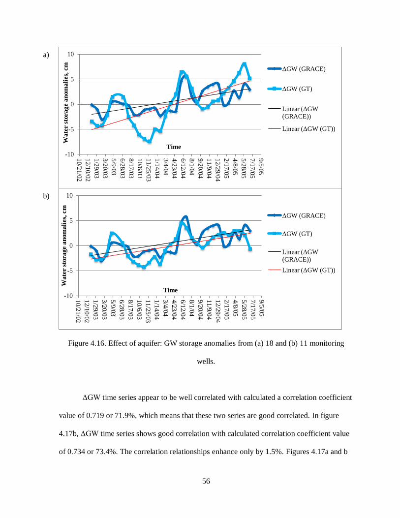
56

Figure 4.16. Effect of aquifer: GW storage anomalies from (a) 18 and (b) 11 monitoring

wells.

ΔGW time series appear to be well correlated with calculated a correlation coefficient

value of 0.719 or 71.9%, which means that these two series are good correlated. In figure

4.17b, ΔGW time series shows good correlation with calculated correlation coefficient value

of 0.734 or 73.4%. The correlation relationships enhance only by 1.5%. Figures 4.17a and b

-10

-5

0

5

10

10

/21

/02

12

/10

/02

1/2

9/0

3

3/2

0/0

3

5/9

/03

6/2

8/0

3

8/1

7/0

3

10

/6/0

3

11

/25

/03

1/1

4/0

4

3/4

/04

4/2

3/0

4

6/1

2/0

4

8/1

/04

9/2

0/0

4

11

/9/0

4

12

/29

/04

2/1

7/0

5

4/8

/05

5/2

8/0

5

7/1

7/0

5

9/5

/05

Wate

r s

tora

ge a

nom

ali

es,

cm

Time

ΔGW (GRACE)

ΔGW (GT)

Linear (ΔGW

(GRACE))

Linear (ΔGW (GT))

-10

-5

0

5

10

10

/21

/02

12

/10

/02

1/2

9/0

3

3/2

0/0

3

5/9

/03

6/2

8/0

3

8/1

7/0

3

10

/6/0

3

11

/25

/03

1/1

4/0

4

3/4

/04

4/2

3/0

4

6/1

2/0

4

8/1

/04

9/2

0/0

4

11

/9/0

4

12

/29

/04

2/1

7/0

5

4/8

/05

5/2

8/0

5

7/1

7/0

5

9/5

/05

Wa

ter s

tora

ge a

nom

ali

es,

cm

Time

ΔGW (GRACE)

ΔGW (GT)

Linear (ΔGW

(GRACE))

Linear (ΔGW (GT))

a)

b)

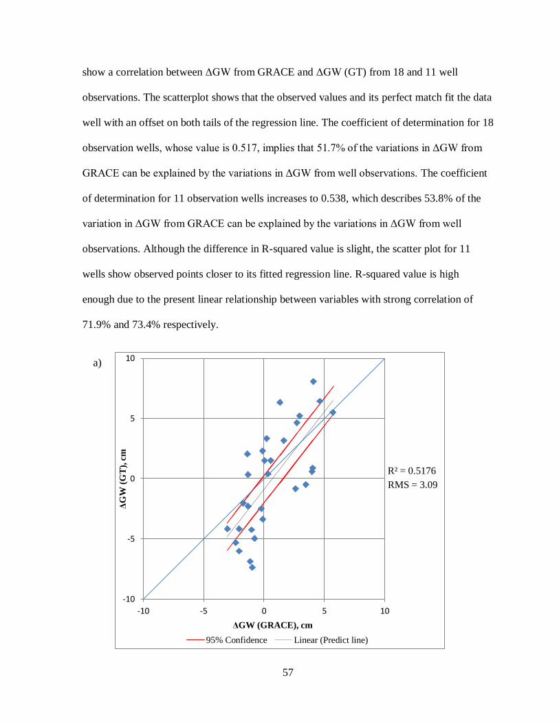
57

show a correlation between ΔGW from GRACE and ΔGW (GT) from 18 and 11 well

observations. The scatterplot shows that the observed values and its perfect match fit the data

well with an offset on both tails of the regression line. The coefficient of determination for 18

observation wells, whose value is 0.517, implies that 51.7% of the variations in ΔGW from

GRACE can be explained by the variations in ΔGW from well observations. The coefficient

of determination for 11 observation wells increases to 0.538, which describes 53.8% of the

variation in ΔGW from GRACE can be explained by the variations in ΔGW from well

observations. Although the difference in R-squared value is slight, the scatter plot for 11

wells show observed points closer to its fitted regression line. R-squared value is high

enough due to the present linear relationship between variables with strong correlation of

71.9% and 73.4% respectively.

R² = 0.5176

-10

-5

0

5

10

-10 -5 0 5 10

ΔG

W (

GT

), c

m

ΔGW (GRACE), cm

95% Confidence Linear (Predict line)

RMS = 3.09

a)

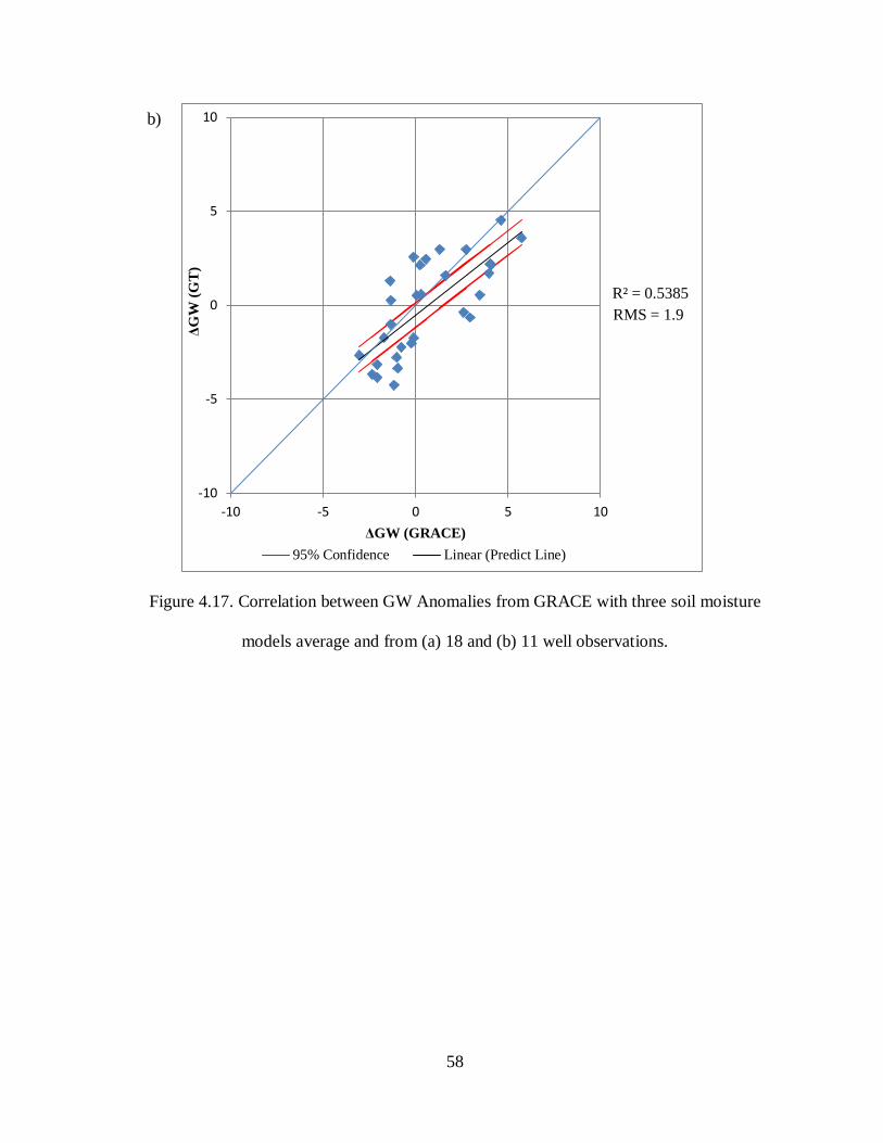
58

Figure 4.17. Correlation between GW Anomalies from GRACE with three soil moisture

models average and from (a) 18 and (b) 11 well observations.

R² = 0.5385

-10

-5

0

5

10

-10 -5 0 5 10

ΔG

W (

GT

)

ΔGW (GRACE)


RMS = 1.9

b)

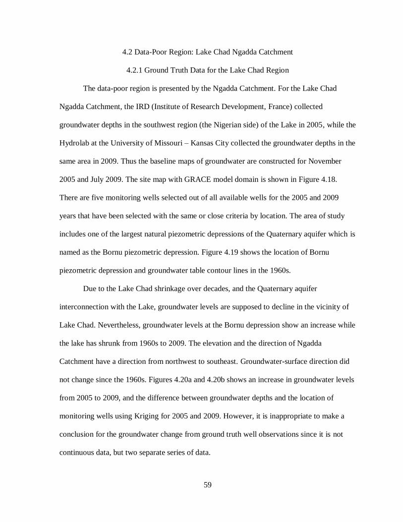
59

4.2 Data-Poor Region: Lake Chad Ngadda Catchment

4.2.1 Ground Truth Data for the Lake Chad Region

The data-poor region is presented by the Ngadda Catchment. For the Lake Chad

Ngadda Catchment, the IRD (Institute of Research Development, France) collected

groundwater depths in the southwest region (the Nigerian side) of the Lake in 2005, while the

Hydrolab at the University of Missouri – Kansas City collected the groundwater depths in the

same area in 2009. Thus the baseline maps of groundwater are constructed for November

2005 and July 2009. The site map with GRACE model domain is shown in Figure 4.18.

There are five monitoring wells selected out of all available wells for the 2005 and 2009

years that have been selected with the same or close criteria by location. The area of study

includes one of the largest natural piezometric depressions of the Quaternary aquifer which is

named as the Bornu piezometric depression. Figure 4.19 shows the location of Bornu

piezometric depression and groundwater table contour lines in the 1960s.

Due to the Lake Chad shrinkage over decades, and the Quaternary aquifer

interconnection with the Lake, groundwater levels are supposed to decline in the vicinity of

Lake Chad. Nevertheless, groundwater levels at the Bornu depression show an increase while

the lake has shrunk from 1960s to 2009. The elevation and the direction of Ngadda

Catchment have a direction from northwest to southeast. Groundwater-surface direction did

not change since the 1960s. Figures 4.20a and 4.20b shows an increase in groundwater levels

from 2005 to 2009, and the difference between groundwater depths and the location of

monitoring wells using Kriging for 2005 and 2009. However, it is inappropriate to make a

conclusion for the groundwater change from ground truth well observations since it is not

continuous data, but two separate series of data.

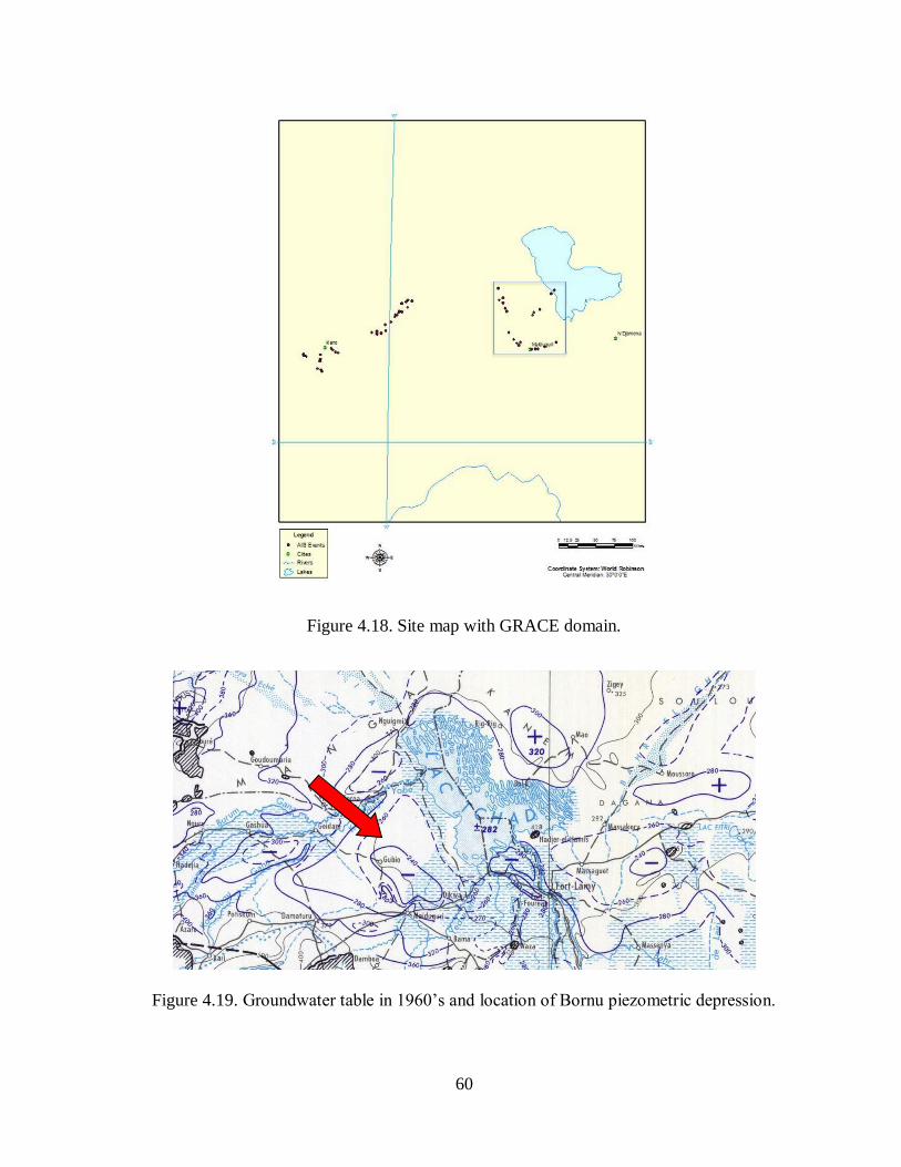
60

Figure 4.18. Site map with GRACE domain.

Figure 4.19. Groundwater table in 1960’s and location of Bornu piezometric depression.

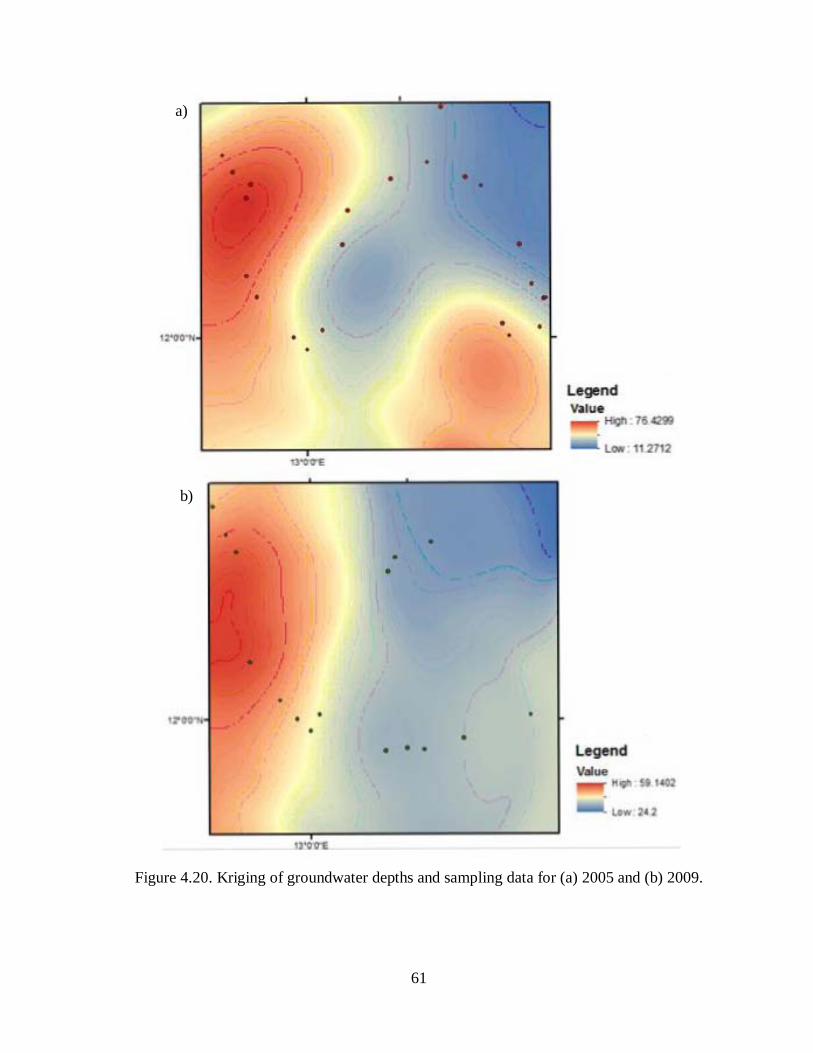
61

Figure 4.20. Kriging of groundwater depths and sampling data for (a) 2005 and (b) 2009.

a)

b)

• •

•

•

• •

• • • • • - ... • 'OIl

62

4.2.2 Effect of Soil Moisture Models

Figure 4.21 depicts the effect of Soil Moisture land surface models on groundwater

variations. In time and space, the period of time is from November 2005 to July 2009 and

over the Lake Chad Ngadda Catchment area. It compares outputs of groundwater changes

derived from GRACE and GLDAS models. Figure 4.21a shows inputs of ΔTWS and ΔSM

and the groundwater storage anomalies ΔGW estimated from GRACE and GLDAS average

soil moisture models. The high picks of seasonal amplitudes occur around September

through November which is a wet season in the region, while low picks represents dry season

from March to May. The seasonal variations of ΔTWS and ΔSM are up to 10 cm. The

seasonal amplitudes reach up to 6 cm for ΔGW estimates. Figures 4.21b, 4.21c, and 4.21d

show inputs of ΔTWS and ΔSM, and ΔGW from GRACE and individual soil moisture

models (CLM, Noah, and Mosaic). CLM soil moisture model shows greater and more stable

fluctuations of groundwater storage anomalies’ ΔGW. High picks fluctuates up to 10 cm.

Mosaic and Noah soil moisture models show similar pattern of groundwater storage changes.

High picks of Mosaic and Noah models almost do not exceed 5 cm. Seasonal amplitudes

fluctuate more often in compare with constant seasonal change of CLM model.

Out of three land surface models, the one with the greatest effect and reasonable

result is the CLM model. The results from CLM model provide the most realistic simulations

of mean annual runoff since the model has a small dynamic range of soil moisture in it.

Mosaic and Noah models show greater soil moisture changes; consequently, groundwater

storage fluctuation would be smaller.

63

4.2.3 Effect of Scales

TWS data derived from GRACE is available only as 1º resolution. However, GLDAS

provides 1º and 0.25º resolution for LSMs. Figure 4.22a shows the groundwater storage

changes computed from 1º TWS and 1º SM, while figure 4.22b shows groundwater storage

changes computed from 1º TWS and 0.25º SM. The pattern of both GRACE-GLDAS

groundwater storage estimates is almost identical with its seasonal amplitudes in wet and dry

seasons. However, groundwater storage anomalies from 0.25º SM gives more detailed

variations.

4.2.4 Effect of Individual Cell

The Lake Chad Ngadda Catchment covers 2º by 2º area of GRACE and GLDAS

spatial resolution. The GRACE approach appears to be appropriate for regions equal or larger

than 5º by 5º area. However, the area cannot be expanded due to the lack of well monitoring

observations. Also, the Lake Chad Ngadda Catchment region covers Bornu piezometric

depression. Therefore, it would be appropriate to look at each individual cell effect. In figure

4.23, a 2º by 2º area is divided into four separate 1º cells for better understanding of each cell

impact. Southeastern and southwestern cells approximately cover the Bornu piezometric

depression. Figures 4.24c and 4.24d show the inputs of GRACE and GLDAS estimates and

output groundwater storage anomalies for southeastern and southwestern cells. The

fluctuations are significantly great in those two cells. Seasonal amplitudes in the wet season

can reach up to 10 cm of groundwater storage anomalies. Figure 4.24a and 4.24b show the

inputs of GRACE and GLDAS estimates and output groundwater storage anomalies for

northeastern and northwestern cells. The fluctuations of groundwater storage changes are half

the size of those in figures 4.24c and 4.24d. Seasonal amplitudes in the wet season reach no

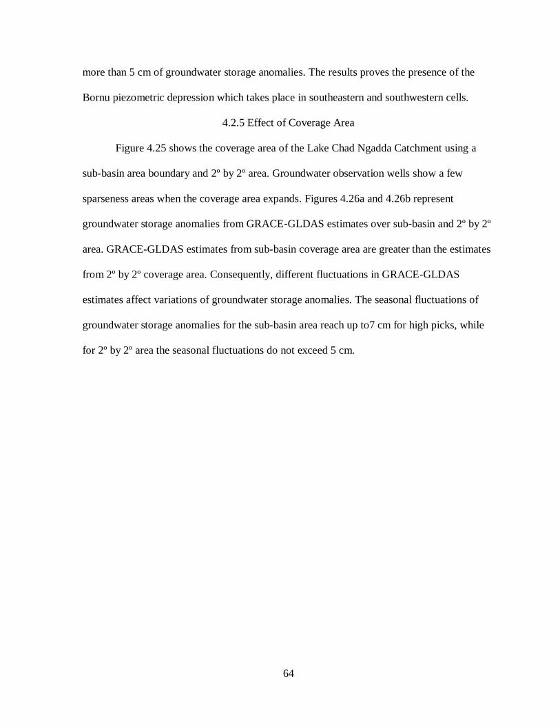
64

more than 5 cm of groundwater storage anomalies. The results proves the presence of the

Bornu piezometric depression which takes place in southeastern and southwestern cells.

4.2.5 Effect of Coverage Area

Figure 4.25 shows the coverage area of the Lake Chad Ngadda Catchment using a

sub-basin area boundary and 2º by 2º area. Groundwater observation wells show a few

sparseness areas when the coverage area expands. Figures 4.26a and 4.26b represent

groundwater storage anomalies from GRACE-GLDAS estimates over sub-basin and 2º by 2º

area. GRACE-GLDAS estimates from sub-basin coverage area are greater than the estimates

from 2º by 2º coverage area. Consequently, different fluctuations in GRACE-GLDAS

estimates affect variations of groundwater storage anomalies. The seasonal fluctuations of

groundwater storage anomalies for the sub-basin area reach up to7 cm for high picks, while

for 2º by 2º area the seasonal fluctuations do not exceed 5 cm.

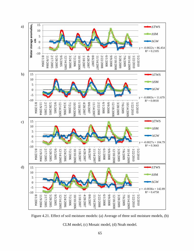
65

Figure 4.21. Effect of soil moisture models: (a) Average of three soil moisture models, (b)

CLM model, (c) Mosaic model, (d) Noah model.

y = -0.0022x + 86.454R² = 0.2105

-10

-5

0

5

10

15

8/1

/20

04

11/9

/2004

2/1

7/2

005

5/2

8/2

00

5

9/5

/2005

12/1

4/2

005

3/2

4/2

006

7/2

/2006

10/1

0/2

006

1/1

8/2

007

4/2

8/2

007

8/6

/2007

11/1

4/2

007

2/2

2/2

008

6/1

/2008

9/9

/2008

12/1

8/2

008

3/2

8/2

009

7/6

/2009

10/1

4/2

009

1/2

2/2

010

5/2

/2010

Wat

er

sto

rage

an

om

alie

s,

cm

ΔTWS

ΔSM

ΔGW

y = -0.0003x + 11.679R² = 0.0018-10

-5

0

5

10

15

8/1

/20

04

11

/9/2

00

4

2/1

7/2

00

5

5/2

8/2

00

5

9/5

/20

05

12

/14

/20

05

3/2

4/2

00

6

7/2

/20

06

10

/10

/20

06

1/1

8/2

00

7

4/2

8/2

00

7

8/6

/20

07

11

/14

/20

07

2/2

2/2

00

8

6/1

/20

08

9/9

/20

08

12

/18

/20

08

3/2

8/2

00

9

7/6

/20

09

10

/14

/20

09

1/2

2/2

01

0

5/2

/20

10

ΔTWS

ΔSM

ΔGW

y = -0.0027x + 104.79R² = 0.3643-10

-5

0

5

10

15

8/1

/20

04

11

/9/2

00

4

2/1

7/2

00

5

5/2

8/2

00

5

9/5

/20

05

12

/14

/20

05

3/2

4/2

00

6

7/2

/20

06

10

/10

/20

06

1/1

8/2

00

7

4/2

8/2

00

7

8/6

/20

07

11

/14

/20

07

2/2

2/2

00

8

6/1

/20

08

9/9

/20

08

12

/18

/20

08

3/2

8/2

00

9

7/6

/20

09

10

/14

/20

09

1/2

2/2

01

0

5/2

/20

10

ΔTWS

ΔSM

ΔGW

y = -0.0036x + 142.89R² = 0.4758-10

-5

0

5

10

15

8/1

/20

04

11

/9/2

004

2/1

7/2

00

5

5/2

8/2

005

9/5

/20

05

12

/14

/2005

3/2

4/2

00

6

7/2

/20

06

10

/10

/2006

1/1

8/2

007

4/2

8/2

00

7

8/6

/20

07

11

/14

/2007

2/2

2/2

008

6/1

/20

08

9/9

/20

08

12

/18

/2008

3/2

8/2

009

7/6

/20

09

10

/14

/2009

1/2

2/2

010

5/2

/20

10

ΔTWS

ΔSM

ΔGW

c)

d)

b)

a)

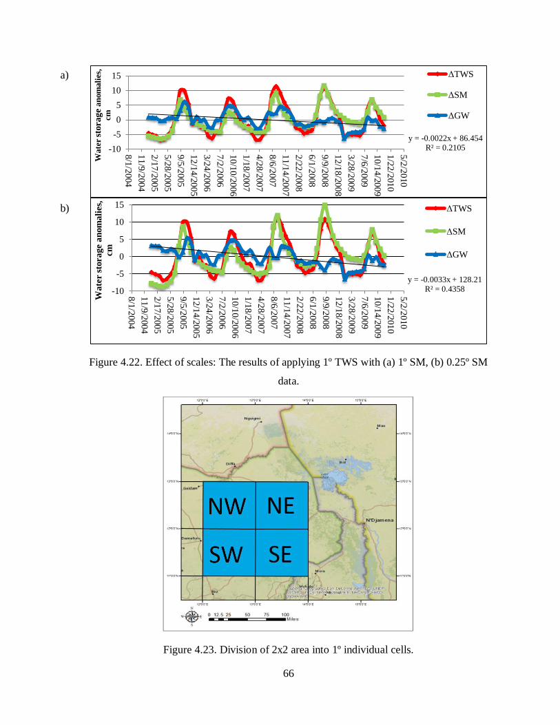
66

Figure 4.22. Effect of scales: The results of applying 1º TWS with (a) 1º SM, (b) 0.25º SM

data.

Figure 4.23. Division of 2x2 area into 1º individual cells.

y = -0.0022x + 86.454R² = 0.2105-10

-5

0

5

10

15

8/1

/2004

11/9

/2004

2/1

7/2

005

5/2

8/2

005

9/5

/2005

12/1

4/2

005

3/2

4/2

006

7/2

/20

06

10/1

0/2

006

1/1

8/2

007

4/2

8/2

007

8/6

/2007

11/1

4/2

007

2/2

2/2

008

6/1

/2008

9/9

/2008

12/1

8/2

008

3/2

8/2

009

7/6

/20

09

10

/14

/20

09

1/2

2/2

010

5/2

/2010

Wate

r s

tora

ge

an

om

ali

es,

cm

ΔTWS

ΔSM

ΔGW

y = -0.0033x + 128.21R² = 0.4358-10

-5

0

5

10

15

8/1

/20

04

11

/9/2

00

4

2/1

7/2

00

5

5/2

8/2

00

5

9/5

/20

05

12

/14

/20

05

3/2

4/2

00

6

7/2

/20

06

10

/10

/20

06

1/1

8/2

00

7

4/2

8/2

00

7

8/6

/20

07

11

/14

/20

07

2/2

2/2

00

8

6/1

/20

08

9/9

/20

08

12

/18

/20

08

3/2

8/2

00

9

7/6

/20

09

10

/14

/20

09

1/2

2/2

01

0

5/2

/20

10

Wa

ter s

torage a

nom

ali

es,

cm

ΔTWS

ΔSM

ΔGW

a)

b)

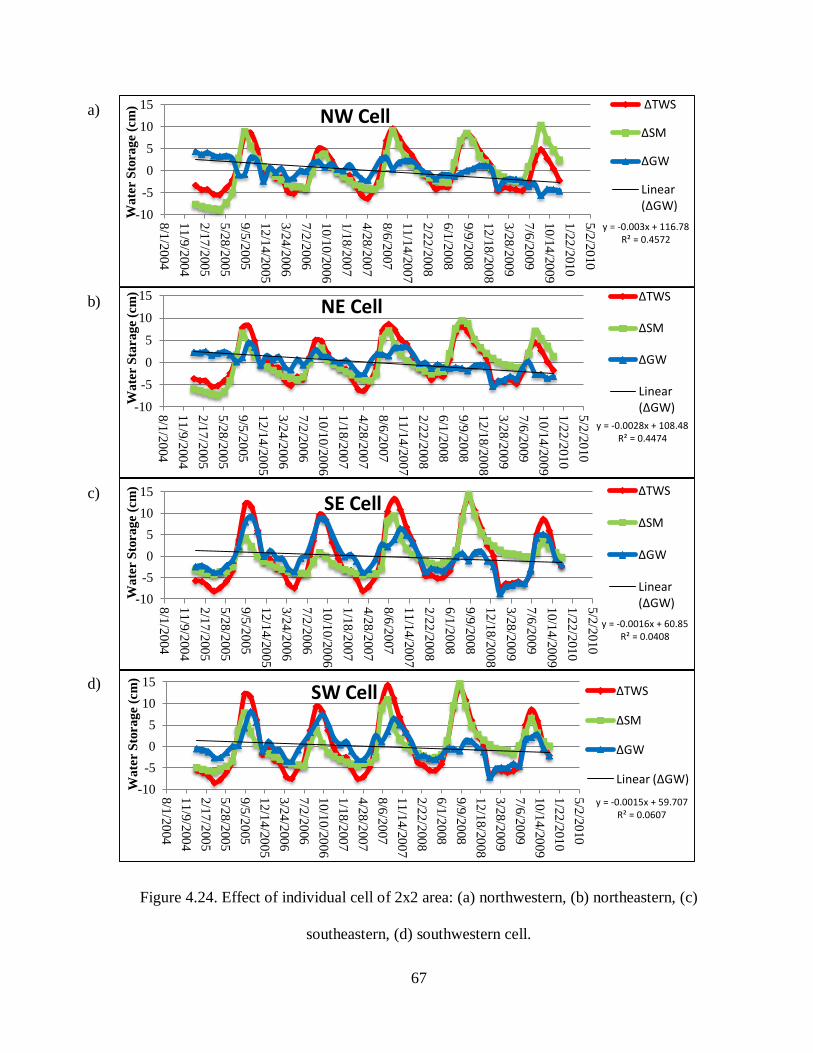
67

Figure 4.24. Effect of individual cell of 2x2 area: (a) northwestern, (b) northeastern, (c)

southeastern, (d) southwestern cell.

y = -0.003x + 116.78R² = 0.4572

-10

-5

0

5

10

15

8/1

/2004

11/9

/2004

2/1

7/2

005

5/2

8/2

00

5

9/5

/2005

12/1

4/2

005

3/2

4/2

006

7/2

/2006

10/1

0/2

006

1/1

8/2

007

4/2

8/2

007

8/6

/2007

11

/14

/20

07

2/2

2/2

008

6/1

/2008

9/9

/2008

12/1

8/2

008

3/2

8/2

009

7/6

/2009

10/1

4/2

009

1/2

2/2

010

5/2

/20

10

Wate

r S

torage (

cm

)NW Cell

ΔTWS

ΔSM

ΔGW

Linear (ΔGW)

y = -0.0028x + 108.48R² = 0.4474

-10

-5

0

5

10

15

8/1

/20

04

11

/9/2

00

4

2/1

7/2

00

5

5/2

8/2

00

5

9/5

/20

05

12

/14

/20

05

3/2

4/2

00

6

7/2

/20

06

10

/10

/20

06

1/1

8/2

00

7

4/2

8/2

00

7

8/6

/20

07

11

/14

/20

07

2/2

2/2

00

8

6/1

/20

08

9/9

/20

08

12

/18

/20

08

3/2

8/2

00

9

7/6

/20

09

10

/14

/20

09

1/2

2/2

01

0

5/2

/20

10

Wa

ter S

tarage (

cm

)

NE CellΔTWS

ΔSM

ΔGW

Linear (ΔGW)

y = -0.0016x + 60.85R² = 0.0408

-10

-5

0

5

10

15

8/1

/20

04

11

/9/2

00

4

2/1

7/2

00

5

5/2

8/2

00

5

9/5

/20

05

12

/14

/20

05

3/2

4/2

00

6

7/2

/20

06

10

/10

/20

06

1/1

8/2

00

7

4/2

8/2

00

7

8/6

/20

07

11

/14

/20

07

2/2

2/2

00

8

6/1

/20

08

9/9

/20

08

12

/18

/20

08

3/2

8/2

00

9

7/6

/20

09

10

/14

/20

09

1/2

2/2

01

0

5/2

/20

10

Wa

ter S

tora

ge (

cm

)

SE CellΔTWS

ΔSM

ΔGW

Linear (ΔGW)

y = -0.0015x + 59.707R² = 0.0607

-10

-5

0

5

10

15

8/1

/20

04

11

/9/2

004

2/1

7/2

00

5

5/2

8/2

005

9/5

/20

05

12

/14

/200

5

3/2

4/2

006

7/2

/20

06

10

/10

/200

6

1/1

8/2

00

7

4/2

8/2

007

8/6

/20

07

11

/14

/200

7

2/2

2/2

008

6/1

/20

08

9/9

/20

08

12

/18

/200

8

3/2

8/2

009

7/6

/20

09

10

/14

/200

9

1/2

2/2

010

5/2

/20

10

Wate

r S

torage (

cm

)

SW Cell ΔTWS

ΔSM

ΔGW

Linear (ΔGW)

b)

a)

c)

d)

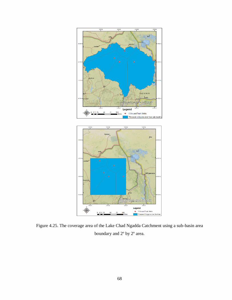
68

Figure 4.25. The coverage area of the Lake Chad Ngadda Catchment using a sub-basin area

boundary and 2º by 2º area.

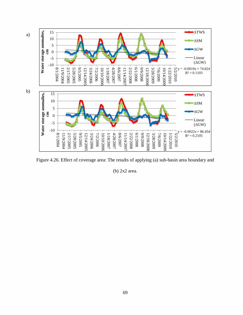
69

Figure 4.26. Effect of coverage area: The results of applying (a) sub-basin area boundary and

(b) 2x2 area.

y = -0.0019x + 74.824R² = 0.1103

-10

-5

0

5

10

15

8/1

/2004

11/9

/2004

2/1

7/2

005

5/2

8/2

00

5

9/5

/2005

12/1

4/2

005

3/2

4/2

006

7/2

/2006

10/1

0/2

006

1/1

8/2

00

7

4/2

8/2

007

8/6

/2007

11/1

4/2

007

2/2

2/2

008

6/1

/2008

9/9

/20

08

12/1

8/2

008

3/2

8/2

009

7/6

/2009

10/1

4/2

009

1/2

2/2

010

5/2

/20

10

Wate

r s

tora

ge a

nom

ali

es,

cm

ΔTWS

ΔSM

ΔGW

Linear

(ΔGW)

y = -0.0022x + 86.454R² = 0.2105

-10

-5

0

5

10

15

8/1

/20

04

11

/9/2

00

4

2/1

7/2

00

5

5/2

8/2

00

5

9/5

/20

05

12

/14

/20

05

3/2

4/2

00

6

7/2

/20

06

10

/10

/20

06

1/1

8/2

00

7

4/2

8/2

00

7

8/6

/20

07

11

/14

/20

07

2/2

2/2

00

8

6/1

/20

08

9/9

/20

08

12

/18

/20

08

3/2

8/2

00

9

7/6

/20

09

10

/14

/20

09

1/2

2/2

01

0

5/2

/20

10

Wa

ter s

tora

ge a

nom

ali

es,

cm

ΔTWS

ΔSM

ΔGW

Linear

(ΔGW)

a)

b)

70

CHAPTER 5

CONCLUSION

We conducted a study to estimate the variations of groundwater using remotely

sensed Gravity Recovery and Climate Experiment and ground truth data. We presented two

case studies of modeling groundwater variations, one in a data-rich region and the other in a

data-poor region. The advantage of using GRACE modeling is that it allows us to determine

groundwater change over a continuous period of time in the region with limited accessibility

to the Basin and a lack of ground truth data.

The Upper Mississippi Basin, as a data-rich region, verified the GRACE efficiency

and accuracy in groundwater change estimations. The simulated results considered the effect

of soil moisture models, groundwater fluctuations in the monitoring well, and the matter of

the aquifer. The most accurate GRACE modeling setup determined the effect of soil moisture

model and aquifer. The results showed that the best fit soil moisture model is CLM. The

calculated correlation coefficient is 86.1%, which signifies strong correlation between remote

sensed and ground truth time series. Also, the results showed that the best selection of well

observations is from a homogeneous aquifer. The results showed that the best fit model is 11

well observations from the same sand and gravel aquifer with strong correlation of 73.4%. I

would like to combine these two well correlated conditions in one case to find the best match

of the data. Figure 5.1 performs the analysis using CLM soil moisture model and selecting 11

well observations from the same aquifer.

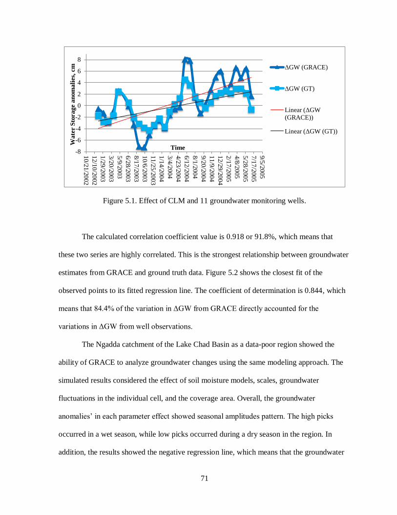
71

Figure 5.1. Effect of CLM and 11 groundwater monitoring wells.

The calculated correlation coefficient value is 0.918 or 91.8%, which means that

these two series are highly correlated. This is the strongest relationship between groundwater

estimates from GRACE and ground truth data. Figure 5.2 shows the closest fit of the

observed points to its fitted regression line. The coefficient of determination is 0.844, which

means that 84.4% of the variation in ΔGW from GRACE directly accounted for the

variations in ΔGW from well observations.

The Ngadda catchment of the Lake Chad Basin as a data-poor region showed the

ability of GRACE to analyze groundwater changes using the same modeling approach. The

simulated results considered the effect of soil moisture models, scales, groundwater

fluctuations in the individual cell, and the coverage area. Overall, the groundwater

anomalies’ in each parameter effect showed seasonal amplitudes pattern. The high picks

occurred in a wet season, while low picks occurred during a dry season in the region. In

addition, the results showed the negative regression line, which means that the groundwater

-8

-6

-4

-2

0

2

4

6

8

10/2

1/2

00

2

12/1

0/2

00

2

1/2

9/2

003

3/2

0/2

003

5/9

/2003

6/2

8/2

003

8/1

7/2

003

10/6

/2003

11/2

5/2

00

3

1/1

4/2

004

3/4

/2004

4/2

3/2

004

6/1

2/2

004

8/1

/2004

9/2

0/2

004

11/9

/2004

12/2

9/2

00

4

2/1

7/2

005

4/8

/2005

5/2

8/2

00

5

7/1

7/2

00

5

9/5

/20

05

Wate

r S

torage a

nom

ali

es,

cm

Time

ΔGW (GRACE)

ΔGW (GT)

Linear (ΔGW

(GRACE))

Linear (ΔGW (GT))

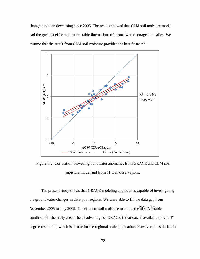
72

change has been decreasing since 2005. The results showed that CLM soil moisture model

had the greatest effect and more stable fluctuations of groundwater storage anomalies. We

assume that the result from CLM soil moisture provides the best fit match.

Figure 5.2. Correlation between groundwater anomalies from GRACE and CLM soil

moisture model and from 11 well observations.

The present study shows that GRACE modeling approach is capable of investigating

the groundwater changes in data-poor regions. We were able to fill the data gap from

November 2005 to July 2009. The effect of soil moisture model is the most valuable

condition for the study area. The disadvantage of GRACE is that data is available only in 1º

degree resolution, which is coarse for the regional scale application. However, the solution in

R² = 0.8443

-10

-5

0

5

10

-10 -5 0 5 10

ΔG

W (

GT

), c

m

ΔGW (GRACE), cm


RMS = 2.2

RMS = 2.2

73

this case would be to use 0.25º degree soil moisture data and downscale it as in the Ngadda

catchment example.

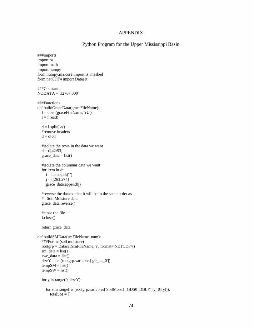
74

APPENDIX

Python Program for the Upper Mississippi Basin

###imports

import os

import math

import numpy

from numpy.ma.core import is_masked

from netCDF4 import Dataset

###Constants

NODATA = '32767.000'

###Functions

def buildGraceData(graceFileName):

f = open(graceFileName, 'rU')

l = f.read()

d = l.split('\n')

#remove headers d = d[6:]

#isolate the rows in the data we want

d = d[42:53]

grace_data = list()

#isolate the columnar data we want

for item in d:

i = item.split(' ')

j = i[263:274]

grace_data.append(j)

#reverse the data so that it will be in the same order as

# Soil Moisture data

grace_data.reverse()

#close the file

f.close()

return grace_data

def buildSMData(smFileName, num):

###For nc (soil moisture) rootgrp = Dataset(smFileName, 'r', format='NETCDF4')

sm_data = list()

swe_data = list()

sizeY = len(rootgrp.variables['g0_lat_0'])

tempSM = list()

tempSW = list()

for y in range(0, sizeY):

for z in range(len(rootgrp.variables['SoilMoist1_GDS0_DBLY'][:][0][y])):

totalSM = []

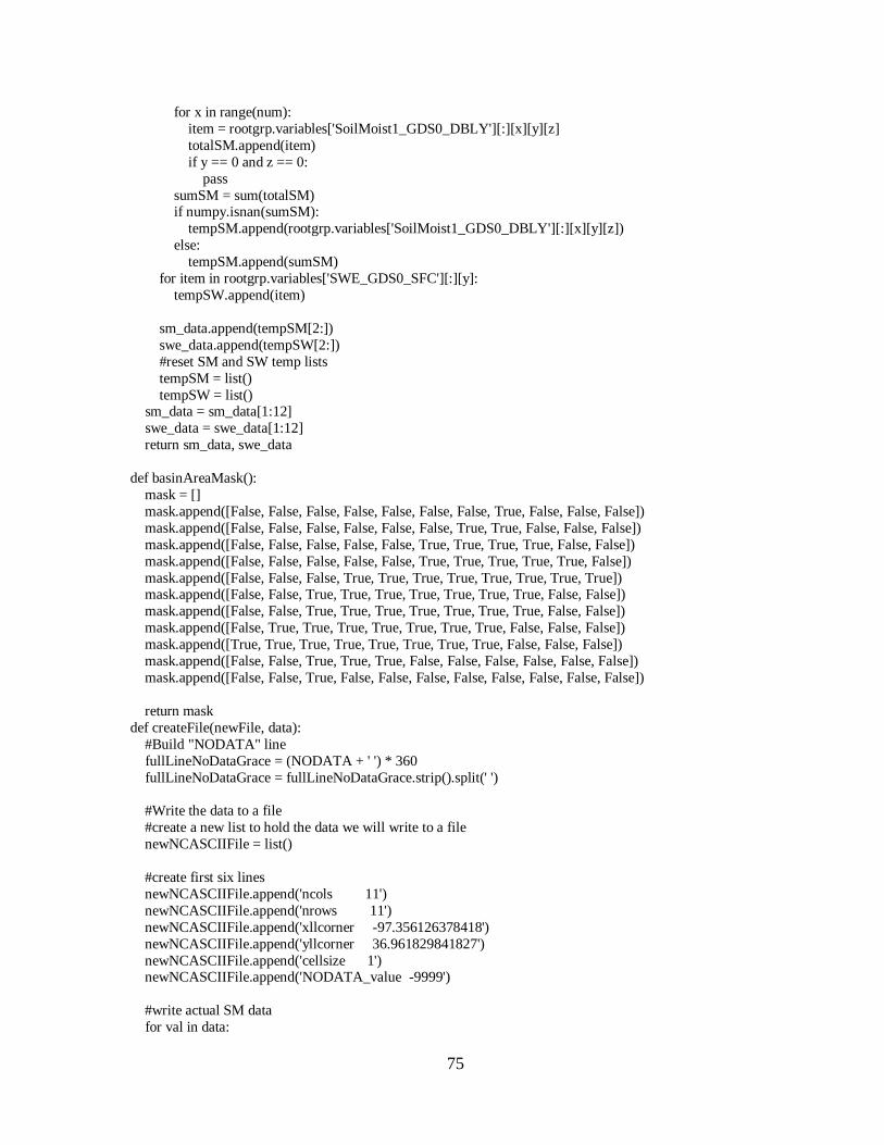
75

for x in range(num):

item = rootgrp.variables['SoilMoist1_GDS0_DBLY'][:][x][y][z]

totalSM.append(item)

if y == 0 and z == 0:

pass

sumSM = sum(totalSM) if numpy.isnan(sumSM):

tempSM.append(rootgrp.variables['SoilMoist1_GDS0_DBLY'][:][x][y][z])

else:

tempSM.append(sumSM)

for item in rootgrp.variables['SWE_GDS0_SFC'][:][y]:

tempSW.append(item)

sm_data.append(tempSM[2:])

swe_data.append(tempSW[2:])

#reset SM and SW temp lists

tempSM = list()

tempSW = list() sm_data = sm_data[1:12]

swe_data = swe_data[1:12]

return sm_data, swe_data

def basinAreaMask():

mask = []

mask.append([False, False, False, False, False, False, False, True, False, False, False])

mask.append([False, False, False, False, False, False, True, True, False, False, False])

mask.append([False, False, False, False, False, True, True, True, True, False, False])

mask.append([False, False, False, False, False, True, True, True, True, True, False])

mask.append([False, False, False, True, True, True, True, True, True, True, True]) mask.append([False, False, True, True, True, True, True, True, True, False, False])

mask.append([False, False, True, True, True, True, True, True, True, False, False])

mask.append([False, True, True, True, True, True, True, True, False, False, False])

mask.append([True, True, True, True, True, True, True, True, False, False, False])

mask.append([False, False, True, True, True, False, False, False, False, False, False])

mask.append([False, False, True, False, False, False, False, False, False, False, False])

return mask

def createFile(newFile, data):

#Build "NODATA" line

fullLineNoDataGrace = (NODATA + ' ') * 360

fullLineNoDataGrace = fullLineNoDataGrace.strip().split(' ')

#Write the data to a file

#create a new list to hold the data we will write to a file

newNCASCIIFile = list()

#create first six lines

newNCASCIIFile.append('ncols 11')

newNCASCIIFile.append('nrows 11')

newNCASCIIFile.append('xllcorner -97.356126378418')

newNCASCIIFile.append('yllcorner 36.961829841827')

newNCASCIIFile.append('cellsize 1') newNCASCIIFile.append('NODATA_value -9999')

#write actual SM data

for val in data:

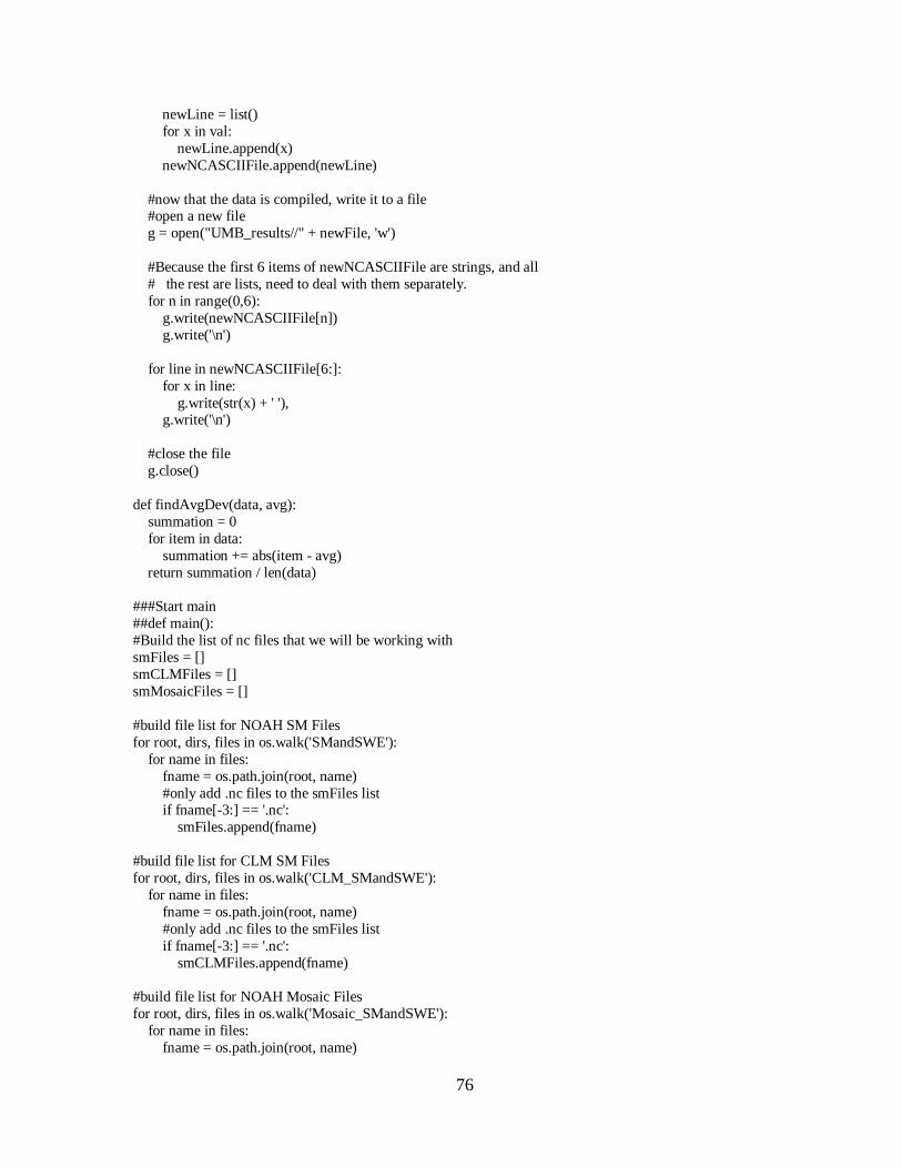
76

newLine = list()

for x in val:

newLine.append(x)

newNCASCIIFile.append(newLine)

#now that the data is compiled, write it to a file #open a new file

g = open("UMB_results//" + newFile, 'w')

#Because the first 6 items of newNCASCIIFile are strings, and all

# the rest are lists, need to deal with them separately.

for n in range(0,6):

g.write(newNCASCIIFile[n])

g.write('\n')

for line in newNCASCIIFile[6:]:

for x in line:

g.write(str(x) + ' '), g.write('\n')

#close the file

g.close()

def findAvgDev(data, avg):

summation = 0

for item in data:

summation += abs(item - avg)

return summation / len(data)

###Start main

##def main():

#Build the list of nc files that we will be working with

smFiles = []

smCLMFiles = []

smMosaicFiles = []

#build file list for NOAH SM Files

for root, dirs, files in os.walk('SMandSWE'):

for name in files:

fname = os.path.join(root, name)

#only add .nc files to the smFiles list if fname[-3:] == '.nc':

smFiles.append(fname)

#build file list for CLM SM Files

for root, dirs, files in os.walk('CLM_SMandSWE'):

for name in files:


#only add .nc files to the smFiles list

if fname[-3:] == '.nc':

smCLMFiles.append(fname)

#build file list for NOAH Mosaic Files

for root, dirs, files in os.walk('Mosaic_SMandSWE'):

for name in files:


77


if fname[-3:] == '.nc':

smMosaicFiles.append(fname)

#Build the list of GRACE data files that we will be working with

graceFiles = []

for root, dirs, files in os.walk('GRACE_data'):

for name in files:


if 'CSR' in fname:

graceFiles.append(fname)

#determine boundaries of data

rootgrp = Dataset(smFiles[0], 'r', format='NETCDF4')

sizeX = 11

sizeY = 11




#Create the ground water "sum" data list

groundWaterData = list()

z = 0


lineList = []

for x in range(0, sizeX):

lineList.append(z) groundWaterData.append(lineList)

#create structures to hold the mean and the average deviation

smAvgDict = {}

swAvgDict = {}

grAvgDict = {}

gwAvgDict = {}

smSTDDict = {}

swSTDDict = {}

grSTDDict = {}

gwSTDDict = {}

smNOAASumDict = {}

smCLMSumDict = {}

smMOSAICSumDict = {}

#create mask file

mask = basinAreaMask()

#process each set of grace and sm files

for smF in smFiles:

smAvg = []

swAvg = []

grAvg = []

gwAvg = []

#determine the year/month of the file from the filename

x = smF.find('_M.A')

tmpDate = smF[x+4:x+10]

78

#find the corresponding grace file, if it exists

for graceF in graceFiles:

if tmpDate in graceF:

#if found, remove it from the graceFiles list so we don't

# have to look at it on the next search

graceFiles.remove(graceF) #once found, stop looking through the graceFiles list

break

for CLMF in smCLMFiles:

if tmpDate in CLMF:

#if found, remove it from the smCLMFiles list so we don't


smCLMFiles.remove(CLMF)

#once found, stop looking through the smCLMFiles list

break

for mosaicF in smMosaicFiles:

if tmpDate in mosaicF: #if found, remove it from the smMosaicFiles list so we don't


#once found, stop looking through the smMosaicFiles list

break

#extract the sm, sw and grace data from the files (the integer is the number of sublayers)

sm, sw = buildSMData(smF, 4)

sm2, sw2 = buildSMData(CLMF, 10)

sm3, sw3 = buildSMData(mosaicF, 3)

##sum up all valid values smTotal = 0

for line in sm:

lineTotal = 0

for item in line:

if not is_masked(item):

lineTotal += item

smTotal += lineTotal

smNOAASumDict[tmpDate] = smTotal

smTotal = 0

for line in sm2:

lineTotal = 0

for item in line: if not is_masked(item):

lineTotal += item


smCLMSumDict[tmpDate] = smTotal

smTotal = 0

for line in sm3:

lineTotal = 0

for item in line:


lineTotal += item

smTotal += lineTotal smMOSAICSumDict[tmpDate] = smTotal

grace = buildGraceData(graceF)

yVals = list()

79


xVals = list()


if mask[y][x]:

#calculate

grAvg.append(float(grace[y][x]))

if is_masked(sm[y][x]):

xVals.append(NODATA)

groundWaterData[y][x] = NODATA

else:

smAvg.append((sm[y][x] + sm2[y][x] + sm3[y][x]) /3 / 10)

calc = float(grace[y][x]) - (((sm[y][x] + sm2[y][x] + sm3[y][x]) /3

+ (sw[y][x] + sw2[y][x] + sw3[y][x])/3) /10.0)

gwAvg.append(calc) xVals.append(calc)

groundWaterData[y][x]+= calc

if not is_masked(sw[y][x]):

swAvg.append((sw[y][x] + sw2[y][x] + sw3[y][x]) /3 /10)

else:

xVals.append(-9999)

yVals.append(xVals)

#calculate and store the average

smAvgDict[tmpDate] = numpy.average(smAvg) swAvgDict[tmpDate] = numpy.average(swAvg)

grAvgDict[tmpDate] = numpy.average(grAvg)

if tmpDate == '200301':

print grAvg

gwAvgDict[tmpDate] = numpy.average(gwAvg)

#calculate and store the average deviation

smSTDDict[tmpDate] = numpy.std(smAvg)

swSTDDict[tmpDate] = numpy.std(swAvg)

grSTDDict[tmpDate] = numpy.std(grAvg)

gwSTDDict[tmpDate] = numpy.std(gwAvg)

#reverse the data so that it will be written to the file in # the correct order

yVals.reverse()

#write data to a file

createFile(tmpDate + '.asc', yVals)

#convert from double-value in groundWaterData to single-value

groundWaterData.reverse()

createFile("ground_water_sum_data.asc", groundWaterData)

#calculate the total average based on all monthly averages for sm and sw totalMeansm = numpy.average(smAvgDict.values())

totalMeansw = numpy.average(swAvgDict.values())

totalMeangw = numpy.average(gwAvgDict.values())

80

keys = smAvgDict.keys()

smDeviation = {}

smDeviation1 = {}

for k in keys:

D = totalMeansm - smAvgDict[k]

D1 = smAvgDict[k] - totalMeansm smDeviation[k] = D

smDeviation1[k] = D1

keys = swAvgDict.keys()

swDeviation = {}

swDeviation1 = {}

for k in keys:

D = totalMeansw - swAvgDict[k]

D1 = swAvgDict[k] - totalMeansw

swDeviation[k] = D

swDeviation1[k] = D1

keys = gwAvgDict.keys()

gwDeviation = {}

gwDeviation1 = {}

for k in keys:

D = totalMeangw - gwAvgDict[k]

D1 = gwAvgDict[k] - totalMeangw

gwDeviation[k] = D

gwDeviation1[k] = D1

#create a file with the averges of all types

f = open('UMB_results//avg.csv', 'w') k = smAvgDict.keys()

k.sort()

#write header row

f.write('Date' + ',' + 'Soil Moisture Avg' + ',' + 'Snow Water Avg' + ',' + 'Grace Avg' +

',' + 'Ground Water Avg' + ',' + 'SM STD' + ',' + 'SW STD' + ',' +

'Grace STD' + ',' + 'GW STD' + ','+ 'SM Total M-Month M' + ',' +

'SW Total m-Month M' + ',' + 'GW Total M-Month M' + ',' +

'SM Month M-Total M' + ',' +'SW Month M-Total M' + ',' + 'GW Month M-Total M' +

',' + 'NOAA SM Sum' + ',' + 'CLM SM Sum' + ',' + 'MOSAIC SM Sum\n')

#write the average (mean) and the average deviation for key in k:

f.write(key[0:4] + '-' + key[4:] + '-' + '01' + ',' + str(smAvgDict[key]) +

',' + str(swAvgDict[key]) + ',' + str(grAvgDict[key]) + ',' + str(gwAvgDict[key]) +

',' + str(smSTDDict[key]) + ',' + str(swSTDDict[key]) + ',' + str(grSTDDict[key]) +

',' + str(gwSTDDict[key]) + ',' + str (smDeviation[key])+

',' + str (swDeviation[key])+ ',' + str (gwDeviation[key]) +

',' + str (smDeviation1[key])+ ',' + str (swDeviation1[key])+

',' + str (gwDeviation1[key]) + ',' + str(smNOAASumDict[key]) + ',' +

str(smCLMSumDict[key]) + ',' + str(smMOSAICSumDict[key]) + '\n')

f.close()

### this is the boilerplate portion

##if __name__ == '__main__':

## main()

81

Python Program for the Ngadda Catchment of the Lake Chad Basin

###imports

import os

import math

import numpy

from numpy.ma.core import is_masked

from netCDF4 import Dataset

###Constants

NODATA = '32767.000'

###Functions

def buildGraceData(graceFileName):

f = open(graceFileName, 'rU')

l = f.read()

d = l.split('\n')

#remove headers

d = d[6:]

#isolate the rows in the data we want

d = d[76:79]

grace_data = list()

#isolate the columnar data we want

for item in d:

i = item.split(' ')

j = i[12:14]

grace_data.append(j)

#reverse the data so that it will be in the same order as

# Soil Moisture data

grace_data.reverse()

#close the file

f.close()

return grace_data

def buildSMData(smFileName, num): ###For nc (soil moisture)

rootgrp = Dataset(smFileName, 'r', format='NETCDF4')

sm_data = list()

swe_data = list()

sizeY = len(rootgrp.variables['g0_lat_0'])

tempSM = list()

tempSW = list()

for y in range(1, sizeY-1):

for z in range(1, len(rootgrp.variables['SoilMoist1_GDS0_DBLY'][:][0][y])-1):

totalSM = []

for x in range(num): item = rootgrp.variables['SoilMoist1_GDS0_DBLY'][:][x][y][z]

82

totalSM.append(item)

if y == 0 and z == 0:

pass

#print item, totalSM

sumSM = sum(totalSM)

if numpy.isnan(sumSM): tempSM.append(rootgrp.variables['SoilMoist1_GDS0_DBLY'][:][x][y][z])

else:

tempSM.append(sumSM)

for item in rootgrp.variables['SWE_GDS0_SFC'][:][y]:

tempSW.append(item)

if item > 0:

print "Snow Water > 0 Detected!"

sm_data.append(tempSM)

swe_data.append(tempSW)

#reset SM and SW temp lists

tempSM = list() tempSW = list()

return sm_data, swe_data

def basinAreaMask():

mask = []

mask.append([True, True])

mask.append([True, True])

mask.append([False, False])

return mask

def createFile(newFile, data):




#Write the data to a file

#create a new list to hold the data we will write to a file

newNCASCIIFile = list()

#create first six lines

newNCASCIIFile.append('ncols 8') newNCASCIIFile.append('nrows 8')

newNCASCIIFile.append('xllcorner 12')

newNCASCIIFile.append('yllcorner 11')

newNCASCIIFile.append('cellsize 0.25')

newNCASCIIFile.append('NODATA_value -9999')

## #create next 41 lines of NODATA

## for n in range(41):

## newNCASCIIFile.append(fullLineNoDataGrace)

#write actual SM data for val in data:

newLine = list()

for x in val:

newLine.append(x)

83

newNCASCIIFile.append(newLine)

#now that the data is compiled, write it to a file

#open a new file

g = open("LCB_results_025//" + newFile, 'w')

#Because the first 6 items of newNCASCIIFile are strings, and all

# the rest are lists, need to deal with them separately.

for n in range(0,6):

g.write(newNCASCIIFile[n])

g.write('\n')

for line in newNCASCIIFile[6:]:

for x in line:

g.write(str(x) + ' '),

g.write('\n')

#close the file g.close()

def findAvgDev(data, avg):

summation = 0

for item in data:

summation += abs(item - avg)

return summation / len(data)

def createGraceCellAvg(fileList):

grace = buildGraceData(fileList[0])

y = len(grace) x = len(grace[0])

avgList = list()

for z in range(y):

tmpList = list()

for w in range(x):

tmpList.append(0)

avgList.append(tmpList)

for f in fileList:

grace = buildGraceData(f)

for z in range(y):

for w in range(x): avgList[z][w] += float(grace[z][w])

numFiles = len(fileList)

for z in range(y):

for w in range(x):

avg = avgList[z][w] / numFiles

avgList[z][w] = avg

print 'grace avg = ', avgList

return avgList

def createSMCellAvg(fileList, numLayers):

sm, sw = buildSMData(fileList[0], numLayers)

y = len(sm)

84

x = len(sm[0])

avgList = list()

for z in range(y):

tmpList = list()

for w in range(x): tmpList.append(0)

avgList.append(tmpList)

for f in fileList:

sm, sw = buildSMData(f, numLayers)

for z in range(y):

for w in range(x):

avgList[z][w] += sm[z][w]

numFiles = len(fileList) for z in range(y):

for w in range(x):

avg = avgList[z][w] / numFiles

avgList[z][w] = avg

print 'avg = ', avgList

print numFiles

return avgList

###Start main

##def main(): #Build the list of nc files that we will be working with

smFiles = []

smCLMFiles = []

smMosaicFiles = []

#build file list for NOAH 0.25 degree SM Files

for root, dirs, files in os.walk('LCB_NOAH_025deg'):

for name in files:



if fname[-3:] == '.nc':

smFiles.append(fname)

#Build the list of GRACE data files that we will be working with

graceFiles = []

for root, dirs, files in os.walk('GRACE_data_LCB'):

for name in files:


if 'CSR' in fname:

graceFiles.append(fname)

graceAvgCellList = createGraceCellAvg(graceFiles)

smAvgCellList = createSMCellAvg(smFiles, 4)

#determine boundaries of data

85

rootgrp = Dataset(smFiles[0], 'r', format='NETCDF4')

sizeX = 8

sizeY = 8

#Create the ground water "sum" data list

groundWaterData = list() z = 0


lineList = []


lineList.append(z)

groundWaterData.append(lineList)

#create structures to hold the mean and the average deviation

smAvgDict = {}

swAvgDict = {}

grAvgDict = {}

gwAvgDict = {} smSTDDict = {}

swSTDDict = {}

grSTDDict = {}

gwSTDDict = {}

smNOAASumDict = {}

#create mask file

mask = basinAreaMask()

#process each set of grace and sm files

for smF in smFiles:

smAvg = []

swAvg = []

grAvg = []

gwAvg = []

#determine the year/month of the file from the filename

x = smF.find('_M.A')

tmpDate = smF[x+4:x+10]

#find the corresponding grace file, if it exists

for graceF in graceFiles: if tmpDate in graceF:

#if found, remove it from the graceFiles list so we don't


graceFiles.remove(graceF)

#once found, stop looking through the graceFiles list

break

#extract the sm, sw and grace data from the files (the integer is the number of sublayers)

sm, sw = buildSMData(smF, 4)

##sum up all valid values

smTotal = 0

for line in sm:

lineTotal = 0

86

for item in line:


lineTotal += item


smNOAASumDict[tmpDate] = smTotal

w = 0

z = 0

grace = buildGraceData(graceF)

yVals = list()


#check if we need to move grace data z position (w,z)

if y == 4:

z+=1

xVals = list()


#check if we need to move grace data w position (w,z) if x == 4:

w+=1

if mask[z][w]:

#calculate

grAvg.append(float(grace[z][w]))

if is_masked(sm[y][x]):

xVals.append(NODATA)

groundWaterData[y][x] = NODATA

else:

smAvg.append((sm[y][x] ) / 10) calc = (float(grace[z][w]) - graceAvgCellList[z][w]) - (((sm[y][x] - smAvgCellList[y][x])

+ sw[y][x]) / 10.0)

gwAvg.append(calc)

xVals.append(calc)

groundWaterData[y][x]+= calc

if not is_masked(sw[y][x]):

swAvg.append(sw[y][x] /10)

else:

xVals.append(-9999) w = 0

yVals.append(xVals)

#calculate and store the average

smAvgDict[tmpDate] = numpy.average(smAvg)

swAvgDict[tmpDate] = numpy.average(swAvg)

grAvgDict[tmpDate] = numpy.average(grAvg)

if tmpDate == '200501':

print '200501 = ', smAvg

gwAvgDict[tmpDate] = numpy.average(gwAvg)

#calculate and store the average deviation

smSTDDict[tmpDate] = numpy.std(smAvg) swSTDDict[tmpDate] = numpy.std(swAvg)

grSTDDict[tmpDate] = numpy.std(grAvg)

gwSTDDict[tmpDate] = numpy.std(gwAvg)

87

#reverse the data so that it will be written to the file in

# the correct order

yVals.reverse()

#write data to a file

createFile(tmpDate + '.asc', yVals) #convert from double-value in groundWaterData to single-value

groundWaterData.reverse()

createFile("ground_water_sum_data.asc", groundWaterData)

#calculate the total average based on all monthly averages for sm and sw

totalMeansm = numpy.average(smAvgDict.values())

totalMeansw = numpy.average(swAvgDict.values())

totalMeangw = numpy.average(gwAvgDict.values())

totalMeangr = numpy.average(grAvgDict.values())

keys = smAvgDict.keys()

smDeviation = {}

smDeviation1 = {}

for k in keys:

D = totalMeansm - smAvgDict[k]

D1 = smAvgDict[k] - totalMeansm

smDeviation[k] = D

smDeviation1[k] = D1

keys = swAvgDict.keys()

swDeviation = {} swDeviation1 = {}

for k in keys:

D = totalMeansw - swAvgDict[k]

D1 = swAvgDict[k] - totalMeansw

swDeviation[k] = D

swDeviation1[k] = D1

keys = gwAvgDict.keys()

gwDeviation = {}

gwDeviation1 = {}

for k in keys:

D = totalMeangw - gwAvgDict[k] D1 = gwAvgDict[k] - totalMeangw

gwDeviation[k] = D

gwDeviation1[k] = D1

keys = grAvgDict.keys()

grDeviation = {}

grDeviation1 = {}

for k in keys:

D = totalMeangr - grAvgDict[k]

D1 = grAvgDict[k] - totalMeangr

grDeviation[k] = D grDeviation1[k] = D1

#create a file with the averges of all types

f = open('LCB_results_025//avg.csv', 'w')

88

k = smAvgDict.keys()

k.sort()

#write header row

f.write('Date' + ',' + 'Soil Moisture Avg' + ',' + 'Snow Water Avg' + ',' + 'Grace Month-M' +

',' + 'Ground Water Avg' + ',' + 'SM STD' + ',' + 'SW STD' + ',' + 'Grace STD' + ',' + 'GW STD' + ','+ 'SM Total M-Month M' + ',' +

'SW Total m-Month M' + ',' + 'GW Total M-Month M' + ',' +

'SM Month M-Total M' + ',' +'SW Month M-Total M' + ',' + 'GW Month M-Total M' +

',' + 'NOAA SM Sum\n')

#write the average (mean) and the average deviation

for key in k:

f.write(key[0:4] + '-' + key[4:] + '-' + '01' + ',' + str(smAvgDict[key]) +

',' + str(swAvgDict[key]) + ',' + str(grDeviation1[key]) + ',' + str(gwAvgDict[key]) +

',' + str(smSTDDict[key]) + ',' + str(swSTDDict[key]) + ',' + str(grSTDDict[key]) +

',' + str(gwSTDDict[key]) + ',' + str (smDeviation[key])+

',' + str (swDeviation[key])+ ',' + str (gwDeviation[key]) + ',' + str (smDeviation1[key])+ ',' + str (swDeviation1[key])+

',' + str (gwDeviation1[key]) + ',' + str(smNOAASumDict[key]) + '\n')

f.close()

### this is the boilerplate portion

##if __name__ == '__main__':

## main()

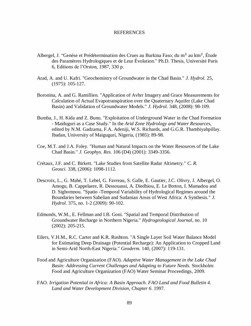
89

REFERENCES

Albergel, J. “Genèse et Prédétermination des Crues au Burkina Faso; du m2 au km2, Étude

des Paramètres Hydrologiques et de Leur Évolution." Ph.D. Thesis, Université Paris

6, Editions de l’Orston, 1987, 330 p.

Arad, A. and U. Kafri. "Geochemistry of Groundwater in the Chad Basin." J. Hydrol. 25,

(1975): 105-127.

Boronina, A. and G. Ramillien. "Application of Avhrr Imagery and Grace Measurements for

Calculation of Actual Evapotranspiration over the Quaternary Aquifer (Lake Chad

Basin) and Validation of Groundwater Models." J. Hydrol. 348, (2008): 98-109.

Bumba, J., H. Kida and Z. Bunu. "Exploitation of Underground Water in the Chad Formation

- Maiduguri as a Case Study." In the Arid Zone Hydrology and Water Resources,

edited by N.M. Gadzama, F.A. Adeniji, W.S. Richards, and G.G.R. Thambiyahpillay.

Ibadan, University of Maiguguri, Nigeria, (1985): 89-98.

Coe, M.T. and J.A. Foley. "Human and Natural Impacts on the Water Resources of the Lake

Chad Basin." J. Geophys. Res. 106 (D4) (2001): 3349-3356.

Crétaux, J.F. and C. Birkett. "Lake Studies from Satellite Radar Altimetry." C. R.

Geosci. 338, (2006): 1098-1112.

Descroix, L., G. Mahé, T. Lebel, G. Favreau, S. Galle, E. Gautier, J.C. Olivry, J. Albergel, O.

Amogu, B. Cappelaere, R. Dessouassi, A. Diedhiou, E. Le Breton, I. Mamadou and

D. Sighomnou. "Spatio -Temporal Variability of Hydrological Regimes around the

Boundaries between Sahelian and Sudanian Areas of West Africa: A Synthesis." J.

Hydrol. 375, no. 1-2 (2009): 90-102.

Edmunds, W.M., E. Fellman and I.B. Goni. "Spatial and Temporal Distribution of

Groundwater Recharge in Northern Nigeria." Hydrogeological Journal, no. 10

(2002): 205-215.

Eilers, V.H.M., R.C. Carter and K.R. Rushton. "A Single Layer Soil Water Balance Model

for Estimating Deep Drainage (Potential Recharge): An Application to Cropped Land

in Semi-Arid North-East Nigeria." Geoderm. 140, (2007): 119-131.

Food and Agriculture Organization (FAO). Adaptive Water Management in the Lake Chad

Basin: Addressing Current Challenges and Adapting to Future Needs. Stockholm:

Food and Agriculture Organization (FAO) Water Seminar Proceedings, 2009.

FAO. Irrigation Potential in Africa: A Basin Approach. FAO Land and Food Bulletin 4.

Land and Water Development Division, Chapter 6. 1997.

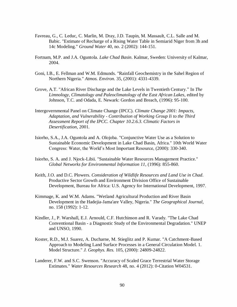
90

Favreau, G., C. Leduc, C. Marlin, M. Dray, J.D. Taupin, M. Massault, C.L. Salle and M.

Babic. "Estimate of Recharge of a Rising Water Table in Semiarid Niger from 3h and

14c Modeling." Ground Water 40, no. 2 (2002): 144-151.

Fortnam, M.P. and J.A. Oguntola. Lake Chad Basin. Kalmar, Sweden: University of Kalmar,

2004.

Goni, I.B., E. Fellman and W.M. Edmunds. "Rainfall Geochemistry in the Sahel Region of

Northern Nigeria." Atmos. Environ. 35, (2001): 4331-4339.

Grove, A.T. "African River Discharge and the Lake Levels in Twentieth Century.” In The

Limnology, Climatology and Paleoclimatology of the East African Lakes, edited by

Johnson, T.C. and Odada, E. Newark: Gordon and Breach, (1996): 95-100.

Intergovernmental Panel on Climate Change (IPCC). Climate Change 2001: Impacts,

Adaptation, and Vulnerability - Contribution of Working Group Ii to the Third

Assessment Report of the IPCC. Chapter 10.2.6.3. Climatic Factors in

Desertification, 2001.

Isiorho, S.A., J.A. Oguntola and A. Olojoba. "Conjunctive Water Use as a Solution to

Sustainable Economic Development in Lake Chad Basin, Africa." 10th World Water

Congress: Water, the World’s Most Important Resource, (2000): 330-340.

Isiorho, S. A. and J. Njock-Libii. "Sustainable Water Resources Management Practice."

Global Networks for Environmental Information 11, (1996): 855-860.

Keith, J.O. and D.C. Plowers. Consideration of Wildlife Resources and Land Use in Chad.

Productive Sector Growth and Environment Division Office of Sustainable

Development, Bureau for Africa: U.S. Agency for International Development, 1997.

Kimmage, K. and W.M. Adams. "Wetland Agricultural Production and River Basin

Development in the Hadejia-Jama'are Valley, Nigeria." The Geographical Journal,

no. 158 (1992): 1-12.

Kindler, J., P. Warshall, E.J. Arnould, C.F. Hutchinson and R. Varady. "The Lake Chad

Conventional Basin - a Diagnostic Study of the Environmental Degradation." UNEP

and UNSO, 1990.

Koster, R.D., M.J. Suarez, A. Ducharne, M. Stieglitz and P. Kumar. "A Catchment-Based

Approach to Modeling Land Surface Processes in a General Circulation Model. 1.

Model Structure." J. Geophys. Res. 105, (2000): 24809-24822.

Landerer, F.W. and S.C. Swenson. "Accuracy of Scaled Grace Terrestrial Water Storage

Estimates." Water Resources Research 48, no. 4 (2012): 0-Citation W04531.

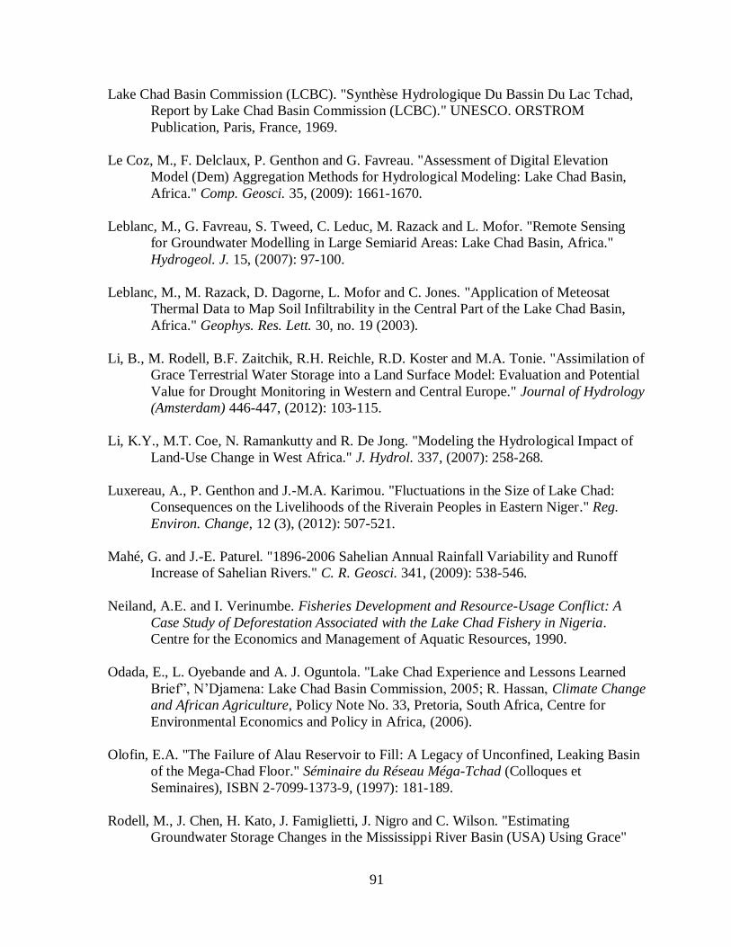
91

Lake Chad Basin Commission (LCBC). "Synthèse Hydrologique Du Bassin Du Lac Tchad,

Report by Lake Chad Basin Commission (LCBC)." UNESCO. ORSTROM

Publication, Paris, France, 1969.

Le Coz, M., F. Delclaux, P. Genthon and G. Favreau. "Assessment of Digital Elevation

Model (Dem) Aggregation Methods for Hydrological Modeling: Lake Chad Basin,

Africa." Comp. Geosci. 35, (2009): 1661-1670.

Leblanc, M., G. Favreau, S. Tweed, C. Leduc, M. Razack and L. Mofor. "Remote Sensing

for Groundwater Modelling in Large Semiarid Areas: Lake Chad Basin, Africa."

Hydrogeol. J. 15, (2007): 97-100.

Leblanc, M., M. Razack, D. Dagorne, L. Mofor and C. Jones. "Application of Meteosat

Thermal Data to Map Soil Infiltrability in the Central Part of the Lake Chad Basin,

Africa." Geophys. Res. Lett. 30, no. 19 (2003).

Li, B., M. Rodell, B.F. Zaitchik, R.H. Reichle, R.D. Koster and M.A. Tonie. "Assimilation of

Grace Terrestrial Water Storage into a Land Surface Model: Evaluation and Potential

Value for Drought Monitoring in Western and Central Europe." Journal of Hydrology

(Amsterdam) 446-447, (2012): 103-115.

Li, K.Y., M.T. Coe, N. Ramankutty and R. De Jong. "Modeling the Hydrological Impact of

Land-Use Change in West Africa." J. Hydrol. 337, (2007): 258-268.

Luxereau, A., P. Genthon and J.-M.A. Karimou. "Fluctuations in the Size of Lake Chad:

Consequences on the Livelihoods of the Riverain Peoples in Eastern Niger." Reg.

Environ. Change, 12 (3), (2012): 507-521.

Mahé, G. and J.-E. Paturel. "1896-2006 Sahelian Annual Rainfall Variability and Runoff

Increase of Sahelian Rivers." C. R. Geosci. 341, (2009): 538-546.

Neiland, A.E. and I. Verinumbe. Fisheries Development and Resource-Usage Conflict: A

Case Study of Deforestation Associated with the Lake Chad Fishery in Nigeria.

Centre for the Economics and Management of Aquatic Resources, 1990.

Odada, E., L. Oyebande and A. J. Oguntola. "Lake Chad Experience and Lessons Learned

Brief”, N’Djamena: Lake Chad Basin Commission, 2005; R. Hassan, Climate Change

and African Agriculture, Policy Note No. 33, Pretoria, South Africa, Centre for

Environmental Economics and Policy in Africa, (2006).

Olofin, E.A. "The Failure of Alau Reservoir to Fill: A Legacy of Unconfined, Leaking Basin

of the Mega-Chad Floor." Séminaire du Réseau Méga-Tchad (Colloques et

Seminaires), ISBN 2-7099-1373-9, (1997): 181-189.

Rodell, M., J. Chen, H. Kato, J. Famiglietti, J. Nigro and C. Wilson. "Estimating

Groundwater Storage Changes in the Mississippi River Basin (USA) Using Grace"

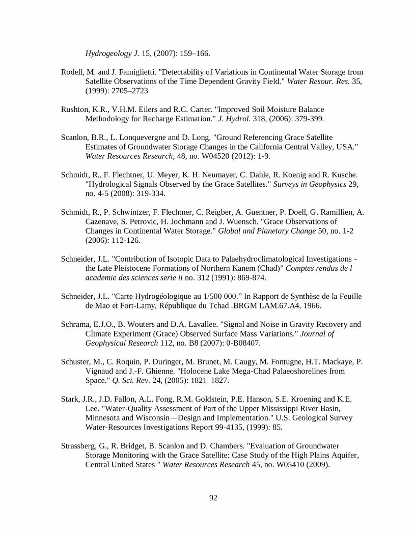
92

Hydrogeology J. 15, (2007): 159–166.

Rodell, M. and J. Famiglietti. "Detectability of Variations in Continental Water Storage from

Satellite Observations of the Time Dependent Gravity Field." Water Resour. Res. 35,

(1999): 2705–2723

Rushton, K.R., V.H.M. Eilers and R.C. Carter. "Improved Soil Moisture Balance

Methodology for Recharge Estimation." J. Hydrol. 318, (2006): 379-399.

Scanlon, B.R., L. Lonquevergne and D. Long. "Ground Referencing Grace Satellite

Estimates of Groundwater Storage Changes in the California Central Valley, USA."

Water Resources Research, 48, no. W04520 (2012): 1-9.

Schmidt, R., F. Flechtner, U. Meyer, K. H. Neumayer, C. Dahle, R. Koenig and R. Kusche.

"Hydrological Signals Observed by the Grace Satellites." Surveys in Geophysics 29,

no. 4-5 (2008): 319-334.

Schmidt, R., P. Schwintzer, F. Flechtner, C. Reigber, A. Guentner, P. Doell, G. Ramillien, A.

Cazenave, S. Petrovic, H. Jochmann and J. Wuensch. "Grace Observations of

Changes in Continental Water Storage." Global and Planetary Change 50, no. 1-2

(2006): 112-126.

Schneider, J.L. "Contribution of Isotopic Data to Palaehydroclimatological Investigations -

the Late Pleistocene Formations of Northern Kanem (Chad)" Comptes rendus de l

academie des sciences serie ii no. 312 (1991): 869-874.

Schneider, J.L. "Carte Hydrogéologique au 1/500 000.” In Rapport de Synthèse de la Feuille

de Mao et Fort-Lamy, République du Tchad .BRGM LAM.67.A4, 1966.

Schrama, E.J.O., B. Wouters and D.A. Lavallee. "Signal and Noise in Gravity Recovery and

Climate Experiment (Grace) Observed Surface Mass Variations." Journal of

Geophysical Research 112, no. B8 (2007): 0-B08407.

Schuster, M., C. Roquin, P. Duringer, M. Brunet, M. Caugy, M. Fontugne, H.T. Mackaye, P.

Vignaud and J.-F. Ghienne. "Holocene Lake Mega-Chad Palaeoshorelines from

Space." Q. Sci. Rev. 24, (2005): 1821–1827.

Stark, J.R., J.D. Fallon, A.L. Fong, R.M. Goldstein, P.E. Hanson, S.E. Kroening and K.E.

Lee. "Water-Quality Assessment of Part of the Upper Mississippi River Basin,

Minnesota and Wisconsin—Design and Implementation." U.S. Geological Survey

Water-Resources Investigations Report 99-4135, (1999): 85.

Strassberg, G., R. Bridget, B. Scanlon and D. Chambers. "Evaluation of Groundwater

Storage Monitoring with the Grace Satellite: Case Study of the High Plains Aquifer,

Central United States " Water Resources Research 45, no. W05410 (2009).

93

Swenson, S., J. Famiglietti, J. Basara and J. Wahr. "Estimating Profile Soil Moisture and

Groundwater Variations Using Grace and Oklahoma Mesonet Soil Moisture Data."

Water Resour. Res. 44, no. W01413, doi: 10.1029/2007WR006057, (2008).

Swenson, S., P. J.-F. Yeh, J. Wahr and J. Famiglietti. "A Comparison of Terrestrial Water

Storage Variations from Grace with in Situ Measurements from Illinois." Geophys.

Res. Lett. 33, no. L16401, doi: 10.1029/2006GL026962, (2006).

Tapley, B.D., S. Bettadpur, J.C. Ries, P.F. Thompson and M.M. Watkins. "Grace

Measurements of Mass Variability in the Earth System." Science 305, (2004): 503–

505.

Thomas, R., M. Meybeck and A. Beim. "Water Quality Assessments - a Guide to Use of

Biota, Sediments and Water in Environmental Monitoring." Chapter 7 – Lakes, edited

by D. Chapman (1992): 325-370.

UN Population Division. "World Populations Prospects: The 2002 Revision Population

Database." Available at: http:// esa.un.org/unpp, (2002).

Wahr, J., S. Swenson, V. Zlotnicki and I. Velicogna. "Time-Variable Gravity from Grace:

First Results." Geophys. Res. Lett. 31, no. L11501, doi: 10.1029/2004GL019779,

(2004).

Wang, X., C. Linage, J. Famiglietti and S.A. Charles. "Gravity Recovery and Climate

Experiment (Grace) Detection of Water Storage Changes in the Three Gorges

Reservoir of China and Comparison with in Situ Measurements." Water Resources

Research 47, no. W12502, doi; 10.1029/2011WR010534, (2011).

Wolf, M. "Direct Measurement of the Earth's Gravitational Potential Using a Satellite Pair."

J. Geophys. Res. 74, no. 22 (1969): 5295-5300.

Xie, P. and P. Arkin. "Global Precipitation: A 17-Year Monthly Analysis Based on Gauge

Observations, Satellite Estimates and Numerical Model Outputs." Bull Am Meteorol.

Soc. 78, (1997): 2539–2558

Zaitchik, B.F., M. Rodell and F. Olivera. "Evaluation of the Global Land Data Assimilation

System Using Global River Discharge Data and a Source-to-Sink Routing Scheme."

Water Resources Research 46, no. W06507, doi: 10.1029/2009WR007811, (2010).

Zaitchik, B. F., M. Rodell and R.H. Reichle. "Assimilation of Grace Terrestrial Water

Storage Data into a Land Surface Model: Results for the Mississippi River Basin."

Journal of Hydrometeorology 9, no. 3 (2008): 535-548.

94

VITA

Alla Skaskevych was born on January 25, 1988 in Pervomaysk, Ukraine. In 2009, she

earned a Bachelor of Science Degree in Computer Environmental and Economic Monitoring

at the Sevastopol National University of Nuclear Energy and Industry, Ukraine. She began

work toward her Master Degree in Environmental and Urban Geosciences at the University

of Missouri-Kansas City, in the fall of 2011. During her research at the University of

Missouri-Kansas City, she participated in the Lake Chad project “Interactions and feedbacks

between biomass burning and water cycle dynamics across the Northern Sub-Saharan

African (NSSA) region” funded by NASA and NSF as a research assistant. Her duty was

conducting groundwater level analysis and geospatial analysis for groundwater, topography,

and land use/land cover. Ms. Alla was awarded the Women Council scholarship in 2014. She

may be reached at [email protected].

Documents

A COMPARISON STUDY OF GRACE-BASED GROUNDWATER …