Embed Size (px)
Citation preview
A COMPARISON OF WAVELET AND SIMPLICITY-BASED HEART SOUND AND
MURMUR SEGMENTATION METHODS
A Thesis
presented to
the Faculty of California Polytechnic State University,
San Luis Obispo
In Partial Fulfillment
of the Requirements for the Degree
Master of Science in Electrical Engineering
by
Joshua David Korven
September 2016

ii
© 2016
Joshua David Korven
ALL RIGHTS RESERVED

iii
COMMITTEE MEMBERSHIP
TITLE: A Comparison of Wavelet and Simplicity-Based
Heart Sound and Murmur Segmentation Methods
AUTHOR: Joshua David Korven
DATE SUBMITTED: September 2016
COMMITTEE CHAIR: Wayne Pilkington, Ph.D.
Associate Professor of Electrical Engineering
COMMITTEE MEMBER: Jane Zhang, Ph.D.
Professor of Electrical Engineering
COMMITTEE MEMBER: John A. Saghri, Ph.D.
Professor of Electrical Engineering

iv
ABSTRACT
A Comparison of Wavelet and Simplicity-Based Heart Sound and Murmur Segmentation
Methods
Joshua David Korven
Stethoscopes are the most commonly used medical devices for diagnosing heart
conditions because they are inexpensive, noninvasive, and light enough to be carried
around by a clinician. Auscultation with a stethoscope requires considerable skill and
experience, but the introduction of digital stethoscopes allows for the automation of this
task. Auscultation waveform segmentation, which is the process of determining the
boundaries of heart sound and murmur segments, is the primary challenge in automating
the diagnosis of various heart conditions. The purpose of this thesis is to improve the
accuracy and efficiency of established techniques for detecting, segmenting, and
classifying heart sounds and murmurs in digitized phonocardiogram audio files. Two
separate segmentation techniques based on the discrete wavelet transform (DWT) and
the simplicity transform are integrated into a MATLAB software system that is capable of
automatically detecting and classifying sound segments.
The performance of the two segmentation methods for recognizing normal heart
sounds and several different heart murmurs is compared by quantifying the results with
clinical and technical metrics. The two clinical metrics are the false negative detection rate
(FNDR) and the false positive detection rate (FPDR), which count heart cycles rather than
sound segments. The wavelet and simplicity methods have a 4% and 9% respective
FNDR, so it is unlikely that either method would not detect a heart condition. However, the
22% and 0% respective FPDR signifies that the wavelet method is likely to detect false
heart conditions, while the simplicity method is not. The two technical metrics are the true

v
murmur detection rate (TMDR) and the false murmur detection rate (FMDR), which count
sound segments rather than heart cycles. Both methods are equally likely to detect true
murmurs given their 83% TMDR. However, the 13% and 0% respective FMDR implies
that the wavelet method is susceptible to detecting false murmurs, while the simplicity
method is not. Simplicity-based segmentation, therefore, demonstrates superior
performance to wavelet-based segmentation, as both are equally likely to detect true
murmurs, but only the simplicity method has no chance of detecting false murmurs.
Keywords: Phonocardiogram, PCG, Stethoscope, Segmentation, Discrete Wavelet
Transform, DWT, Simplicity Transform, Beamforming
vi
TABLE OF CONTENTS
Page
LIST OF TABLES .......................................................................................................... xii
LIST OF FIGURES ....................................................................................................... xiv
CHAPTER
1 INTRODUCTION ........................................................................................................ 1
1.1 Cardiac Structure and Function ............................................................................ 1
1.2 Cardiac Cycle ...................................................................................................... 3
1.3 Auscultation, Heart Sounds, & Murmurs .............................................................. 4
1.4 Heart Sound and Murmur Segmentation Goals .................................................... 9
1.5 Literature Review ............................................................................................... 10
1.6 Proposed Modifications to the Established Methods .......................................... 12
2 VIABILITY OF USING A STETHOSCOPE ARRAY FOR IMPROVED HEART
SOUND DETECTION ............................................................................................... 14
2.1 Introduction ........................................................................................................ 14
2.2 Multiple Input Stethoscope ................................................................................. 14
2.3 Beamforming ..................................................................................................... 15
2.4 Acoustic Aperture............................................................................................... 16
2.5 Directivity Pattern ............................................................................................... 18
2.6 Aperture Array ................................................................................................... 19
2.7 Beamforming ..................................................................................................... 20
2.8 Simulation Results ............................................................................................. 22
2.9 Discussion ......................................................................................................... 30
3 SEGMENTATION ALGORITHMS AND CONCEPTS ................................................ 31
3.1 Frequency Domain Filtering ............................................................................... 31

vii
3.2 Wavelet Transform ............................................................................................. 35
3.2.1 Continuous Wavelet Transform ................................................................ 35
3.2.2 Discrete Wavelet Transform ..................................................................... 36
3.3 Simplicity Transform .......................................................................................... 37
3.3.1 Complexity and Simplicity ........................................................................ 37
3.3.2 Dynamical Systems ................................................................................. 39
3.3.3 The Method of Delays .............................................................................. 40
3.3.4 Eigenvalue Decomposition and the Singular Spectrum ............................ 43
3.3.5 Shannon Entropy ..................................................................................... 44
3.4 Piecewise Constant Denoising ........................................................................... 47
3.5 Potts Functional ................................................................................................. 53
4 SEGMENTATION SYSTEM IMPLEMENTATION ..................................................... 56
4.1 System Overview ............................................................................................... 56
4.1.1 Introduction .............................................................................................. 56
4.1.2 Properties and Methods ........................................................................... 56
4.1.3 PCG Retrieval .......................................................................................... 61
4.1.4 Wavelet filtering ....................................................................................... 62
4.1.5 Segmentation .......................................................................................... 65
4.1.6 Storing and summarizing results .............................................................. 67
4.1.7 Displaying results ..................................................................................... 69
4.2 Wavelet-based Segmentation ............................................................................ 71
4.2.1 Heart Sound Segmentation ...................................................................... 71
4.2.2 Removing Murmurs from Heart Sound Segments .................................... 76
4.2.3 Separating Split Heart Sounds ................................................................. 79
4.2.4 Heart Cycle Segmentation ....................................................................... 81
4.2.5 Murmur Segmentation ............................................................................. 83
viii
4.2.6 Heart Sound and Murmur Classification ................................................... 84
4.3 Simplicity-based Segmentation .......................................................................... 87
4.3.1 Simplicity Waveform Filtering ................................................................... 87
4.3.2 Piecewise Constant Approximation .......................................................... 88
4.3.3 Heart Sound and Murmur Segmentation .................................................. 91
4.3.4 Split Sound Detection, Heart Cycle Segmentation, and Sound
Segment Classification ............................................................................ 92
5 SEGMENTATION RESULTS .................................................................................... 94
5.1 Introduction ........................................................................................................ 94
5.1.1 Sound File Datasets ................................................................................ 94
5.1.2 Segmentation Errors and Detection Rates ............................................... 94
5.1.3 False Negative and False Positive Detection Rates ................................. 96
5.2 Wavelet-Based Segmentation ............................................................................ 99
5.2.1 Wavelet Constants ................................................................................... 99
5.2.2 Wavelet Errors ....................................................................................... 100
5.2.3 Wavelet Results ..................................................................................... 114
5.3 Simplicity-Based Segmentation ........................................................................ 117
5.3.1 Simplicity Constants............................................................................... 117
5.3.2 Simplicity Errors ..................................................................................... 117
5.3.3 Simplicity Error Tables ........................................................................... 126
5.4 Comparison of Segmentation Error Performance for the Two Methods ............ 129
6 CONCLUSIONS AND FUTURE WORK .................................................................. 133
REFERENCES ............................................................................................................ 135
APPENDICES
A. Scripts ............................................................................................................. 140
A.1 Examples ............................................................................................... 140
ix
A.1.1 chp4_seg.m .................................................................................... 140
A.1.2 energy_functions.m ........................................................................ 140
A.1.3 heart_sounds.m .............................................................................. 141
A.1.4 PCG_FFT.m ................................................................................... 142
A.1.5 PCG_simpl.m ................................................................................. 143
A.1.6 rect_sinc.m ..................................................................................... 143
A.1.7 singular_spectra.m ......................................................................... 144
A.2 Results .................................................................................................. 145
A.2.1 batch.m .......................................................................................... 145
A.2.2 beamforming.m .............................................................................. 146
A.2.3 dwt_michigan.m ............................................................................. 147
A.2.4 dwt_littmann.m ............................................................................... 147
A.2.5 simpl_michigan.m ........................................................................... 148
A.2.6 simpl_littmann.m ............................................................................ 149
B. Functions ......................................................................................................... 151
B.1 Beamforming ......................................................................................... 151
B.1.1 beam_pattern.m ............................................................................. 151
B.1.2 beamform.m ................................................................................... 152
B.1.3 dist_mat.m ...................................................................................... 153
B.1.4 isAliased.m ..................................................................................... 153
B.2 DWT ...................................................................................................... 154
B.2.1 coef_plot.m ..................................................................................... 154
B.2.2 coef_rng.m ..................................................................................... 155
B.3 Main ....................................................................................................... 155
B.3.1 batch_segment.m ........................................................................... 155
B.3.2 find_heart_cycles.m ....................................................................... 156

x
B.3.3 katz_fd.m ........................................................................................ 158
B.3.4 lbl_sounds.m .................................................................................. 159
B.3.5 levels2seg.m .................................................................................. 162
B.3.6 limit_HS.m ...................................................................................... 163
B.3.7 load_PCG.m ................................................................................... 164
B.3.8 peak_peel.m ................................................................................... 166
B.3.9 split_HS.m ...................................................................................... 167
B.3.10 st.m .............................................................................................. 169
B.4 Miscellaneous ........................................................................................ 170
B.4.1 closest.m ........................................................................................ 170
B.4.2 energy.m ........................................................................................ 171
B.4.3 env.m ............................................................................................. 171
B.4.4 nfft.m .............................................................................................. 171
B.4.5 normalize.m .................................................................................... 172
B.4.6 pcg_descr.m ................................................................................... 172
B.4.7 rect.m ............................................................................................. 172
B.4.8 shannon_energy.m ......................................................................... 172
B.4.9 smooth.m ....................................................................................... 173
B.4.10 time.m .......................................................................................... 174
B.5 Plotting .................................................................................................. 174
B.5.1 fmt_line_arg.m................................................................................ 174
B.5.2 horiz_line.m .................................................................................... 175
B.5.3 plot_style.m .................................................................................... 175
B.5.4 vert_line.m ...................................................................................... 175
C. Class Definitions and Methods ......................................................................... 176
C.1 @segment ............................................................................................. 176

xi
C.1.1 combine.m ..................................................................................... 176
C.1.2 find.m ............................................................................................. 176
C.1.3 levels.m .......................................................................................... 177
C.1.4 mask.m .......................................................................................... 177
C.1.5 segment.m ..................................................................................... 177
C.1.6 signal.m.......................................................................................... 178
C.1.7 split.m ............................................................................................ 179
C.2 @stethoscope ........................................................................................ 179
C.2.1 cmp_PCG.m .................................................................................. 179
C.2.2 dwt_filt.m ........................................................................................ 180
C.2.3 dwt_segment.m .............................................................................. 180
C.2.4 plot.m ............................................................................................. 185
C.2.5 print.m ............................................................................................ 187
C.2.6 simpl_segment.m ........................................................................... 188
C.2.7 stethoscope.m ................................................................................ 192
C.2.8 title.m ............................................................................................. 196

xii
LIST OF TABLES
Table Page
Table 4-1: stethoscope.m constant properties (SetAccess = immutable). ...................... 60
Table 4-2: stethoscope.m constant properties (SetAccess = public). ............................. 60
Table 4-3: stethoscope.m data properties (SetAccess = private). .................................. 61
Table 4-4: Set of all possible keys for conditions. .......................................................... 68
Table 4-5: Example keys and values for sscope.conditions. .......................................... 68
Table 4-6: Heart sound and murmur segment color codes for plot(sscope). .................. 70
Table 5-1: False negatives (Michigan). .......................................................................... 97
Table 5-2: False positives (Michigan). ........................................................................... 97
Table 5-3: False negatives (Littmann). ........................................................................... 98
Table 5-4: False positives (Littmann). ............................................................................ 98
Table 5-5: False negative detection rates (FNDR). ........................................................ 99
Table 5-6: False positive detection rates (FPDR). ......................................................... 99
Table 5-7: FNDR and FPDR comparison for wavelet and simplicity-based
segmentation. ................................................................................................................ 99
Table 5-8: Wavelet constants. ..................................................................................... 100
Table 5-9: Wavelet-based segmentation error labels and descriptions. ....................... 114
Table 5-10: Wavelet-based segmentation results (Michigan). ...................................... 115
Table 5-11: Wavelet-based segmentation results (Littmann). ...................................... 116
Table 5-12: Wavelet-based segmentation true murmur detection rate (TMDR). .......... 116
Table 5-13: Wavelet-based segmentation false murmur detection rate (FMDR). ......... 116
Table 5-14: Simplicity-based segmentation constants. ................................................ 117
Table 5-15: Simplicity-based segmentation error labels and descriptions. ................... 126
Table 5-16: Simplicity-based segmentation results (Michigan). ................................... 127

xiii
Table 5-17: Simplicity-based segmentation results (Littmann). .................................... 128
Table 5-18: Simplicity true murmur detection rate (TMDR). ......................................... 128
Table 5-19: Simplicity false murmur detection rate (FMDR). ........................................ 128
Table 5-20: Wavelet and simplicity-based segmentation performance
comparison. ................................................................................................................. 129
Table 5-21: Wavelet and simplicity-based segmentation error comparisons
(Michigan). .................................................................................................................. 131
Table 5-22: Wavelet and simplicity-based segmentation error comparisons
(Littmann) .................................................................................................................... 132

xiv
LIST OF FIGURES
Figure Page
Figure 1-1: Blood flow through the heart (oxygen-poor blood is blue, oxygen-rich
blood is red). Adapted from [2]......................................................................................... 1
Figure 1-2: The heart’s chambers, veins, arteries, and valves [2]. ................................... 2
Figure 1-3: Diastole and systole [4]. ................................................................................ 4
Figure 1-4: Labeled stethoscope [5]. ............................................................................... 5
Figure 1-5: Phonocardiogram of a healthy heart [heart_sounds.m]. ................................. 6
Figure 1-6: PCG with a split S2 [heart_sounds.m]. .......................................................... 7
Figure 1-7: PCG with an S3 [heart_sounds.m]. ................................................................ 8
Figure 1-8: PCG with an S4 [heart_sounds.m]. ................................................................ 9
Figure 2-1: Precordial landmarks: Aortic (A), Pulmonic (P), Erb’s point (E),
Tricuspid (T), and Mitral (M) [6]. ..................................................................................... 14
Figure 2-2: Spherical coordinate system [23]. ................................................................ 18
Figure 2-3: Stethoscope positions in the apparatus [beamforming.m]. ........................... 22
Figure 2-4: Steering Φ between 0 and π (f = 500 Hz, no spatial aliasing). ..................... 25
Figure 2-5: Steering Φ between 0 and π (f = 7 kHz, no spatial aliasing). ....................... 27
Figure 2-6: Steering Φ between 0 and π (f = 20 kHz, spatial aliasing). .......................... 29
Figure 3-1: PCG spectrum [PCG_FFT.m]. ..................................................................... 34
Figure 3-2: Fourier transform of the sinc function [rect_sinc.m]. .................................... 38
Figure 3-3: Singular spectra comparison [singular_spectra.m]. ..................................... 44
Figure 3-4: Raw simplicity waveform [PCG_simpl.m]. .................................................... 48
Figure 3-5: Low pass filtering a rectangle causes ripple. The signal at the right
was filtered with a higher order LPF than the signal at the left [31]. ............................... 49

xv
Figure 4-1: A range of approximation coefficients (left subplots) and detail
coefficients (right subplots) are used to determine which approximation
coefficient is optimal for PCG reconstruction [chp4_seg.m]. .......................................... 64
Figure 4-2: The original PCG (top subplot) has very little noise, so the filtered
PCG (bottom subplot) appears similar to the original PCG [chp4_seg.m]. ..................... 65
Figure 4-3: Graphical segmentation results for a PCG with systolic murmurs and
split S2 [chp4_seg.m]. ................................................................................................... 70
Figure 4-4: Shannon energy vs squared energy [energy_functions.m]. ......................... 72
Figure 4-5: Two peak peeling iterations. Subplot-1 separates the input signal into
the peak signal (blue) and the rejected signal (red). Subplot-2 displays the
current output signal, which is a sum of the peaks from the current and previous
iterations [chp4_seg.m]. ................................................................................................ 74
Figure 4-6: PCG (subplot-1), wavelet reconstructed PCG (subplot-2), and peak
peeled Shannon energy with overlaid constant threshold (subplot-3)
[chp4_seg.m]. ................................................................................................................ 76
Figure 4-7: Final heart cycle and heart sound segment boundaries overlaid on
the original PCG (subplot-1), troughs and thresholds for removing murmur
samples from heart sound segments (subplot-2), murmur samples removed from
heart sound segments (subplot-3), and segmented murmurs (subplot-4)
[chp4_seg.m]. ................................................................................................................ 78
Figure 4-8: A heart sound segment containing split heart sounds is separated
into its component segments (subplot-3) [chp4_seg.m]. ................................................ 80
Figure 4-9: The heart cycle boundary locations are approximated from spikes in
the autocorrelation of the PCG’s envelope (subplot-1). Afterwards, the cycle
boundaries are shifted right and aligned with the nearest heart sound segment
start indices (subplot-2) [chp4_seg.m]. .......................................................................... 83
xvi
Figure 4-10: The peak peeled fractal dimension extracts the sound peaks from
the background noise (subplot-2), which are used to zero the non-sound
segments in the raw simplicity waveform (subplot-4) [chp4_seg.m]. .............................. 90
Figure 4-11: Threshold the normal heart sounds, extra heart sounds, and murmur
segments by their simplicity levels (subplot-2) [chp4_seg.m]. ........................................ 92
Figure 5-1: The first S1 is mistaken for a murmur because its maximum energy is
less than the energy threshold (subplot-3) [dwt_michigan.m]. ..................................... 102
Figure 5-2: The first S1 segment is misidentified as a murmur, but the second S1
segment is properly identified (subplot-4). As a result, the first heart cycle’s start
boundary is moved from S1 to the nearest S2 (subplot-1) [dwt_michigan.m]. .............. 103
Figure 5-3: The first S4 is misidentified as a murmur because its maximum
energy is less than the energy threshold (subplot-3) [dwt_littmann.m]. ........................ 105
Figure 5-4: The first S4 is misidentified as a murmur, but the second S4 is
acceptably misidentified as a split sound component (subplot-4). The cycle
boundary locations are correct because S1 and S2 are properly identified
(subplot-1) [dwt_littmann.m]. ....................................................................................... 106
Figure 5-5: The diastolic murmur is misidentified as a heart sound because its
maximum energy is greater than the threshold (subplot-3) [dwt_littmann.m]................ 108
Figure 5-6: The S4 peaks are below the segment thresholds (subplot-2) and are
therefore misidentified as murmurs (subplot-4) [dwt_michigan.m]. .............................. 110
Figure 5-7: The opening snap murmur is misidentified as a split S2 component
because the murmur’s peak is above the threshold (subplot-2). Also, the right
boundary of S1 is repositioned despite the lack of a systolic murmur, and the
remaining piece is misidentified as a murmur [dwt_michigan.m]. ................................. 112
Figure 5-8: The cycle durations are too short because a peak near zero lag is
misidentified as a heart cycle boundary [“AP.mp3”, dwt_littmann.m]. .......................... 113
xvii
Figure 5-9: The diastolic murmur is misidentified as a heart sound because its
simplicity levels are greater than the HS threshold (subplot-2) [simpl_littmann.m]. ...... 119
Figure 5-10: No heart sounds are detected because all segment levels are less
than the HS threshold (subplot-5) [simpl_littmann.m]. .................................................. 121
Figure 5-11: The low amplitude diastolic murmurs (not visible) are undetected
because they were zeroed while peak peeling the fractal dimension (subplot-2).
The corresponding simplicity values are zeroed (subplot-4), so the murmurs are
not segmented (subplot-5) [simpl_michigan.m]. ........................................................... 123
Figure 5-12: The summation gallops are misidentified as split sound components
because their simplicity levels are less than the extra HS threshold (subplot-2).
This causes systole and diastole, and therefore S1 and S2, to be switched
(subplot-1) [simpl_littmann.m]. ..................................................................................... 125

1
1 Introduction
1.1 Cardiac Structure and Function
The purpose of the heart is to circulate blood throughout the body and supply the vital
organs with oxygen, route the blood flow through the lungs to enrich the blood with oxygen,
and dispose of the CO2 waste collected from the body. The most basic functional
breakdown of the heart is to separate it into a right and a left side. Right and left are relative
to the observer’s own frame of reference, so the orientation is reversed when the heart is
presented on a diagram. The right side receives CO2-laden, oxygen-poor blood from the
body and sends it to the lungs for CO2 removal and oxygen enrichment. Conversely, the
left side receives oxygen-rich blood from the lungs and sends it to the rest of the body for
oxygen distribution and CO2 waste collection. This process is synchronous because the
left and right sides send and receive blood in unison [1]. The flow of blood through both
sides of the heart is illustrated in Figure 1-1.
Figure 1-1: Blood flow through the heart (oxygen-poor blood is blue, oxygen-rich blood is red).
Adapted from [2].

2
The two sides of the heart are separated by a muscular wall called the septum. Each
side of the heart is further subdivided into two chambers, of which there are two types:
atria and ventricles. The atria are the upper chambers that collect blood, and the ventricles
are the lower chambers that pump blood. The heart has four chambers in total because
each side has an atrium and a ventricle [1].
Blood enters the heart through veins and exits through arteries. The right atrium
collects CO2-laden waste blood from the body through the venae cavae, where blood from
the upper body flows through the superior vena cava, and blood from the lower body flows
through the inferior vena cava. The right ventricle then sends the waste blood to the lungs
through the pulmonary artery. At the same time, the left atrium collects oxygen-rich blood
from the lungs through the pulmonary vein and sends the oxygen-rich blood to the body
through the aorta. The heart’s chambers, veins, and arteries are labeled in Figure 1-2.
Figure 1-2: The heart’s chambers, veins, arteries, and valves [2].

3
The heart is able to pump blood because valves separate the chambers and enable
pressure gradients to form. Valves are passive structures made of connective tissue rather
than muscle and are shaped like leaflets. The leaflet structure allows pressure differences
alone to open or close valves, and it ensures that blood flows in a single direction without
backflow into a previous chamber. A valve with leaflets pointing into a chamber will snap
shut when the chamber’s pressure exceeds the surrounding environment. Likewise, a
valve with leaflets protruding from a chamber will open when the chamber’s pressure
exceeds the surrounding environment.
The atria and ventricles are separated by the atrioventricular valves: the tricuspid
valve separates the right atrium and right ventricle, while the mitral valve (bicuspid valve)
separates the left atrium and left ventricle. Likewise, the ventricles and arteries are
separated by the semilunar valves: the pulmonary valve separates the right ventricle and
pulmonary artery, while the aortic valve separates the left ventricle and aorta. The four
valves are labeled in Figure 1-2.
1.2 Cardiac Cycle
The cardiac cycle is divided into two distinct phases: diastole and systole. Diastole
occurs when the ventricles relax and blood fills the atria (filling phase), while systole occurs
when the ventricles contract and pump blood into the arteries (ejection phase) [3].
Diastole begins after the ventricles expel blood into the arteries, and the semilunar
valves snap shut due to the arterial pressure exceeding ventricular pressure. At the same
time, atrial pressure exceeds ventricular pressure, so blood returning from the body flows
through the atrioventricular valves and fills the ventricles. The majority of the blood
reaches the ventricles passively, but the atria eventually contract and force any remaining
blood into the ventricles.
4
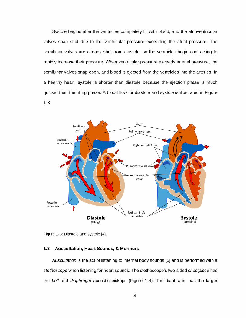
Systole begins after the ventricles completely fill with blood, and the atrioventricular
valves snap shut due to the ventricular pressure exceeding the atrial pressure. The
semilunar valves are already shut from diastole, so the ventricles begin contracting to
rapidly increase their pressure. When ventricular pressure exceeds arterial pressure, the
semilunar valves snap open, and blood is ejected from the ventricles into the arteries. In
a healthy heart, systole is shorter than diastole because the ejection phase is much
quicker than the filling phase. A blood flow for diastole and systole is illustrated in Figure
1-3.
Figure 1-3: Diastole and systole [4].
1.3 Auscultation, Heart Sounds, & Murmurs
Auscultation is the act of listening to internal body sounds [5] and is performed with a
stethoscope when listening for heart sounds. The stethoscope’s two-sided chestpiece has
the bell and diaphragm acoustic pickups (Figure 1-4). The diaphragm has the larger

5
circumference and is used for listening to higher pitched sounds, while the bell has the
smaller circumference and is used for listening to lower pitched sounds [5]. However,
modern stethoscopes often have a tunable diaphragm, instead of a bell, which can be
adjusted for both low and high pitched sounds.
Figure 1-4: Labeled stethoscope [5].
Normal heart sounds associated with systole and diastole are audible during
auscultation when closing heart valves vibrate against the chambers of the heart and
radiate sound throughout the chest (opening valves are inaudible) [1]. The first normal
heart sound, S1, occurs at the beginning of systole when the atrioventricular valves snap
shut; and the second normal heart sound, S2, occurs at the beginning of diastole when
the semilunar valves snap shut. In addition to the normal heart sounds, extra heart sounds
may occur during diastole. If blood strikes a non-compliant left ventricle during passive
filling, then an extra S3 sound occurs shortly after the normal S2; and if the blood ejected
by the left atrium at the end of diastole also strikes a non-compliant left ventricle, then an
extra S4 sound occurs shortly before the S1 that starts the next systole phase.
Unlike heart sounds, murmurs are sounds that are caused by the disruption of laminar
blood flow rather than the closing of heart valves, and are induced through four primary

6
means: narrowing of valves (stenosis), backflow through bad valves (valve insufficiency
or “regurgitation”), irregular flow between chambers (septal defect), and high volume flow
[6]. Murmurs are typically named after the heart valve or chamber where the defect occurs,
for example: aortic stenosis (AS), mitral regurgitation (MR), atrial septal defect (ASD), etc.
For this thesis, describing the murmurs as either systolic or diastolic is sufficient.
A phonocardiogram (PCG) is a recording of a heart sound’s intensity over time [7],
which is illustrated in Figure 1-5 for a healthy heart. A PCG makes it possible to
algorithmically detect and classify the heart sounds and murmurs.
Figure 1-5: Phonocardiogram of a healthy heart [heart_sounds.m].
In a phonocardiogram, S1 is typically louder (higher amplitude) than S2 due to the
higher pressure on the left side of the heart. However, the relative intensities are
sometimes switched, particularly in the elderly, so this feature cannot be used to reliably
distinguish S1 from S2. Instead, systole and diastole are determined by comparing the
distances between unidentified heart sounds, where systole is shorter than diastole
because blood ejects from the ventricles more rapidly than it fills the ventricles. Since S1
7
is the beginning of systole, and S2 is the beginning of diastole, S1 and S2 can therefore
be identified by their temporal locations and spacing rather than by their intensities.
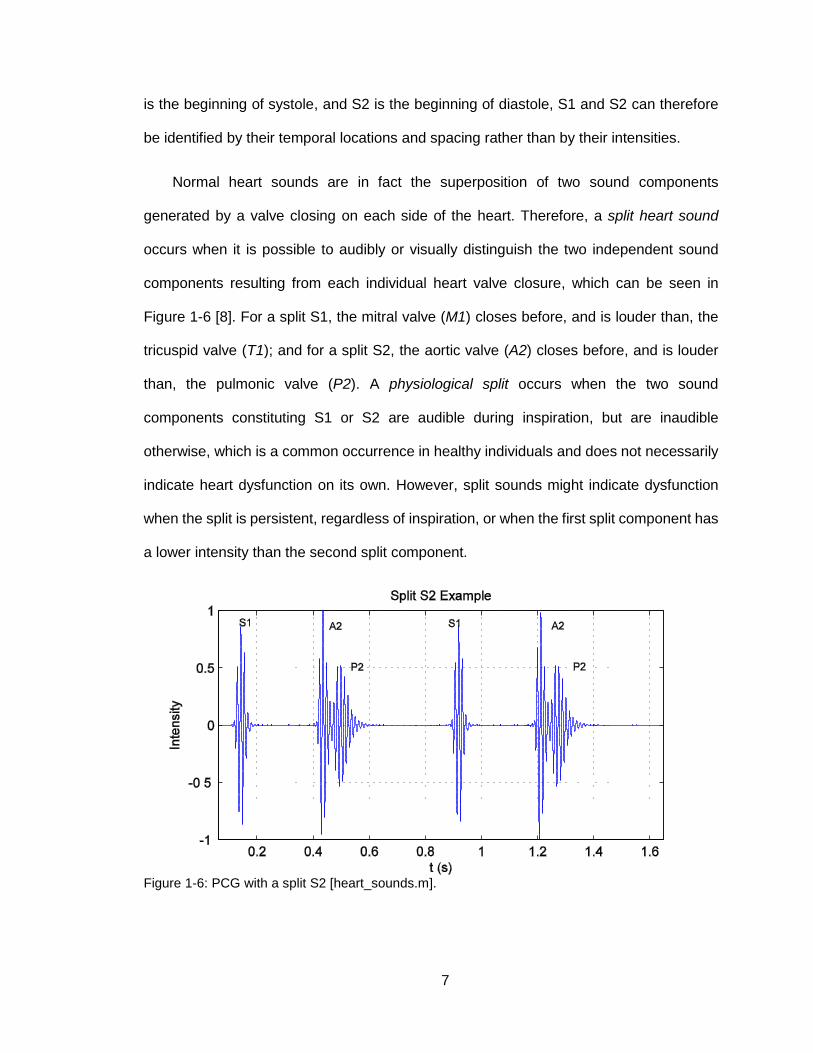
Normal heart sounds are in fact the superposition of two sound components
generated by a valve closing on each side of the heart. Therefore, a split heart sound
occurs when it is possible to audibly or visually distinguish the two independent sound
components resulting from each individual heart valve closure, which can be seen in
Figure 1-6 [8]. For a split S1, the mitral valve (M1) closes before, and is louder than, the
tricuspid valve (T1); and for a split S2, the aortic valve (A2) closes before, and is louder
than, the pulmonic valve (P2). A physiological split occurs when the two sound
components constituting S1 or S2 are audible during inspiration, but are inaudible
otherwise, which is a common occurrence in healthy individuals and does not necessarily
indicate heart dysfunction on its own. However, split sounds might indicate dysfunction
when the split is persistent, regardless of inspiration, or when the first split component has
a lower intensity than the second split component.
Figure 1-6: PCG with a split S2 [heart_sounds.m].

8
Since S3 occurs shortly after S2, and S4 occurs shortly before S1, it is often difficult
to distinguish S3 and S4 from split sound components. However, both of these sounds
typically have lower frequencies and lower intensities than S1 and S2, so it is possible to
identify them through careful auscultation or visual analysis of the PCG. S3 can be seen
in Figure 1-7, and S4 can be seen in Figure 1-8. It is also important to note that S3 and
S4 are ignored when determining S1 and S2 by comparing the distances between
unidentified normal heart sounds.
Figure 1-7: PCG with an S3 [heart_sounds.m].

9
Figure 1-8: PCG with an S4 [heart_sounds.m].
Murmurs are distinguishable from heart sounds because they have higher pitches
and are irregularly shaped compared to heart sounds. If murmurs are present, they exist
in the time periods between S1 and S2, and are therefore classified as either systolic or
diastolic. They are further categorized by their relative durations and locations within
systole or diastole as either early, mid, late, or holo-systolic/diastolic murmurs (“holo”
murmurs occupy the entire systole or diastole).
1.4 Heart Sound and Murmur Segmentation Goals
The primary purpose of this thesis is to improve the accuracy and efficiency of
established techniques for detecting and segmenting heart sounds and murmurs. Since
the sounds are nonstationary events, the first challenge is distinguishing sound segments
from background noise, which is accomplished through a process known as peak peeling.
In general, the peaks extracted through peak peeling do not necessarily represent a single
sound segment since heart sounds and murmurs are often merged into a single peak. For
example, ejection murmurs are initiated shortly after S1, and holosystolic murmurs span
the entirety of systole, so both of these murmurs blur the boundaries between heart

10
sounds and murmurs. Also, split heart sounds with multiple peaks are sometimes difficult
to detect through peak peeling alone. As a result, additional techniques must be developed
for accurately segmenting heart sounds and murmurs, irrespective of their proximities to
other sounds.
In addition to locating the segment boundaries, this thesis attempts to classify the
specific type of each sound segment. Central to this objective is using the normal heart
sounds S1 and S2 as markers for locating the heart cycle boundaries and distinguishing
systole from diastole. In particular, the heart cycle boundaries are located by cross
correlating the signal with itself (autocorrelation) [9] and then aligning the boundaries with
the nearest S1 or S2 segment for greater accuracy. Isolating the heart cycles allows for
systole and diastole, and hence S1 and S2, to be identified on a cycle-by-cycle basis.
Finally, the murmurs can be located within systole or diastole and classified accordingly.
1.5 Literature Review
Various methods have been established for detecting heart sounds and murmurs, but
this thesis in particular extends established wavelet and simplicity-based segmentation
techniques.
The peak peeling algorithm introduced by Hadjileontiadis and Rekanos [10] [11] was
developed for the purpose of extracting explosive lung and bowel sound segments from
the background noise. It is most effective at detecting these transient sound peaks when
applied to the fractal dimension of the PCG, which is a positive-valued signal that is a
measure of time domain complexity. In particular, the fractal dimension attenuates noise
significantly (including noise that is typically unfilterable through standard linear
processing techniques) but transforms the actual sounds into prominent peaks. Peak
peeling is sufficient for accurately segmenting explosive lung and bowel sound peaks due
to their characteristic crescendo-decrescendo shape, which tends to produce distinct start

11
and stop boundaries. When multiple sounds are merged into a single peak, a second peak
peeling iteration is typically sufficient for separating the sounds, as the crescendo-
decrescendo shape tends to produce a deep, distinct trough, even between merged
peaks. Peak peeling is likewise effective at segmenting normal heart sounds given their
similar morphology to explosive lung and bowel sounds. However, it is ineffective at
detecting merged heart sounds and murmurs because murmurs that begin immediately
after S1 or S2 do not produce a deep enough trough for a second iteration to reliably
separate the peaks.
A rudimentary wavelet-based segmentation technique is proposed by Atanasov and
Ning [12]. The purpose of the discrete wavelet transform (DWT) here is to attenuate the
higher frequency murmurs but not the lower frequency heart sounds. The peaks are then
analyzed in the filtered PCG’s energy waveform, where the non-attenuated peaks are
identified as heart sound segments. In practice, the attenuated murmurs will have a small,
but non-zero, energy value, so a threshold is used to distinguish peaks from non-peaks.
After segmenting the heart sounds, the unfiltered PCG’s energy waveform is used to
segment the murmurs. This straightforward approach is acceptable as long as the
murmurs are attenuated sufficiently, which is the case here because the demonstrated
murmurs exhibit ideal attenuation.
The simplicity transform detailed by Nigam and Priemer [13] forms the basis of an
amplitude and energy-invariant segmentation technique that is implemented by Kumar et
al [14]. The simplicity is an inverse measure of signal complexity that is obtained by
embedding the time domain signal into a higher dimensional state space representation,
so that the state space dimension can be used to estimate signal complexity. Unlike the
fractal dimension, each sound segment has an approximately constant simplicity value,
or level, which allows for accurate identification of segment boundaries and sound type.

12
In particular, simplicity-based segmentation can distinguish between heart sounds,
murmurs, and noise because heart sounds have higher simplicity levels than murmurs,
while noise has the lowest possible simplicity level.
1.6 Proposed Modifications to the Established Methods
The wavelet-based segmentation method proposed by Atanasov and Ning is
problematic because it assumes that all murmurs are sufficiently attenuated after filtering,
so that each peak encompasses a single heart sound segment. However, some of the
murmurs examined in this thesis are only partially attenuated after filtering, so certain
peaks may only contain murmurs, while others may contain both heart sounds and
murmurs. Therefore, three improvements are proposed for wavelet-based segmentation.
The first applies a threshold to the filtered energy waveform to remove any partially
attenuated, low energy murmur peaks. The second searches the remaining peaks for
troughs that might indicate merged heart sounds and murmurs, and if found, removes the
murmurs. The third uses peak peeling to detect the heart sound and murmur segment
boundaries with greater accuracy. In particular, the heart sounds are segmented by
peeling the filtered energy waveform, while the murmurs are segmented by peeling the
fractal dimension of the original PCG.
The simplicity-based segmentation method proposed by Kumar et al, despite offering
a marked performance improvement over wavelet-based segmentation, is also
problematic in certain regards. This is primarily a result of the simplicity waveform’s
imperfect resemblance to a piecewise constant function, where the simplicity values in
each segment do not form a constant level, and the transitions between levels are not
instantaneous. This is acceptable when the sound segments are disconnected, as each
segment’s level can be approximated by its average simplicity value, but is ineffective
when heart sounds and murmurs are merged into a single peak. Instead, the simplicity

13
waveform’s piecewise constant approximation can be determined through a process
known as piecewise constant denoising, the theory of which is detailed by Little and Jones
[15]. The particular denoising algorithm used in this thesis is implemented in the MATLAB
toolbox Pottslab by Storath et al [16] [17] [18]. Another drawback of simplicity-based
segmentation is the computational cost incurred by embedding the time domain signal into
state space, which involves multiplying matrices that are proportional in size to number of
samples in the analyzing window. Since the sound segments are only intermittent events,
calculating the simplicity for all samples in the PCG is inefficient. In this thesis, the sound
peaks are first extracted from the background noise by peak peeling, so that the simplicity
only has to be calculated within sound segment boundaries.

14
2 Viability of Using a Stethoscope Array for Improved Heart Sound Detection
2.1 Introduction
A stethoscope is a single element passive acoustic sensor that receives sound waves
from the body. Heart sounds and murmurs are best heard when the chestpiece of the
stethoscope is placed on one of five precordial landmarks on the chest (Figure 2-1). The
aortic (A), pulmonic (P), tricuspid (T), and mitral (M) landmarks are the optimal listening
locations for their associated valves. Thus, S1 is best heard at the tricuspid and mitral
areas, while S2 is best heard at the aortic and pulmonic areas. The fifth landmark, Erb’s
point (E), evenly splits the sound between S1 and S2 [19].
Figure 2-1: Precordial landmarks: Aortic (A), Pulmonic (P), Erb’s point (E), Tricuspid (T), and
Mitral (M) [6].
The five precordial landmarks are optimized for auscultating certain murmurs but are
nonetheless corrupted by sounds from other locations in the heart and the rest of the body.
2.2 Multiple Input Stethoscope
A multiple input stethoscope is proposed by Wong in [20] to improve the signal to
noise ratio (SNR) of a PCG. Of interest here is whether or not such a multi-sensor
configuration could provide an improved PCG waveform for segmentation and heart sound

15
detection by applying beamforming techniques to focus the stethoscope’s acoustic
sensitivity on a smaller region within the heart from which murmur sounds originate.
Beamforming, focusing, and steering of a detector’s sensitivity requires multiple sensors,
and its feasibility depends on the number, size, and physical arrangement of the sensors;
as well as the frequency and location of the sound source, and the physical properties of
the medium between the source and the sensors.
In the proposed multiple input stethoscope array, each stethoscope diaphragm is
secured to a supportive apparatus so that the sensors contact all five landmarks when the
fixture is secured to the patient’s chest. Straps are used to secure the apparatus to the
patient since manually holding the device corrupts the signal with noise.
After collecting the data, a cross correlation is performed over all possible pairs of
input signals (32 total) to align heart sound features in each of the five signals. Cross
correlation is a procedure whereby two signals, offset in time relative to each other, are
multiplied together sample-by-sample and then summed. The process continues until both
signals are correlated at every possible offset, where one signal is fixed in time while the
other advances by a single sample per correlation. The five signals are then aligned where
the correlation is the greatest, and summing the aligned signals averages out the noise
and improves the PCG’s SNR.
2.3 Beamforming
The acoustic pickup of a stethoscope receives sound waves incident from many
directions. The elements of the stethoscope array are situated closest to the five listening
locations, but nonetheless receive unwanted sounds from other areas of the body. The
coherent averaging technique is an effective solution to reduce noise and enhance the
quality of heart sounds in a PCG; however, data collection and processing occur
independently—the sensors are only synchronized to start and stop together but otherwise
16
operate independently until the data is collected. An improved method, namely, beam
steering or beamforming, uses the relative locations of the five sensors and the wave
speed to electronically “steer” the beam pattern towards the sound source.
A useful tool to understand wave reception is the beam pattern or directivity pattern.
The directivity pattern is a spherical plot that displays a field’s intensity as a function of
incident angle. When sound propagates from multiple locations, the wave fronts produce
a field pattern of peaks and troughs caused by constructive and destructive interference.
Knowing this, a sensor array can alter its directivity pattern by applying a phase offset to
each element to either constructively or destructively align the beam pattern in a particular
direction. This allows heart signals originating from different directions to be collected and
analyzed separately, rather than averaged together.
2.4 Acoustic Aperture
An aperture is a region in space that transmits or receives propagating waves [21, p.
3]. A digital stethoscope is a passive aperture that only receives acoustic waves as
opposed to an ultrasound machine, which is an array of active apertures that both sends
and receives acoustic waves to image the internal organs [22]. Thus, only passive
apertures are considered for this thesis. A propagating acoustic wave is described by its
intensity, or sound pressure, 𝑥(𝑡, 𝐫) as a function of time and position; alternatively, the
wave can be described by its Fourier transformed intensity 𝑋(𝑓, 𝐫) as a function of
frequency and position. The aperture function, or sensitivity function, 𝐴(𝑓, 𝐫) relates the
wave intensity incident on the aperture, 𝑋(𝑓, 𝐫), to the wave intensity received by the
aperture, 𝑋𝑅(𝑓, 𝐫) [21, p. 3]:
𝑋𝑅(𝑓, 𝐫) = 𝐴(𝑓, 𝐫)𝑋(𝑓, 𝐫)
where the position vector 𝐫 = [𝑥 𝑦 𝑧]T is relative to the sound source location.

17
The wave equation is a general formula that describes the propagation of acoustic
and electromagnetic waves, among other types of waves [21, p. 2]:
∇2𝑥(𝑡, 𝐫) −1
𝑐2𝛿2
𝛿𝑡2𝑥(𝑡, 𝐫) = 0
An acoustic wave resembles a spherical wave front in the near field, which is close to the
origin of transmission [21, p. 6]. As the wave propagates into the far field, the profile
flattens and approximates a planar wave front. The distinction between the near field and
far field is dependent upon wavelength, aperture shape, and distance from the source to
the aperture. The wave equation has both near field (planar) and far field (spherical)
solutions [21, p. 2]:
𝑥(𝑡, 𝐫) = 𝐴𝑒𝑗(𝜔𝑡−𝐤⋅𝐫) (planar)
𝑥(𝑡, 𝐫) = −𝐴
4𝜋𝑟𝑒𝑗(𝜔𝑡−𝐤⋅𝐫) (spherical)
where the wavenumber:
𝐤 =2𝜋
𝜆[𝑠𝑖𝑛𝜃𝑐𝑜𝑠𝜙 𝑠𝑖𝑛𝜃𝑠𝑖𝑛𝜙 𝑐𝑜𝑠𝜃]
is a vector relative to the sound source location that is oriented along the direction of wave
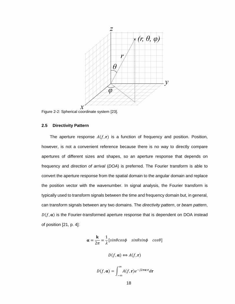
propagation and that measures the spatial wave density [21, p. 2]. The direction is
specified as an angle, so each element in the vector is shown as a conversion from
spherical to rectangular coordinates. Spherical coordinates are comprised of the (𝑟, 𝜃, 𝜙)
dimensions, where 𝑟 is the magnitude, 𝜃 is the polar angle, and 𝜙 is the azimuthal angle,
as shown in Figure 2-2. The phase shift given by the dot product 𝐤 ⋅ 𝐫 is maximized when
the position vector is aligned with the direction of wave propagation.
18
Figure 2-2: Spherical coordinate system [23].
2.5 Directivity Pattern
The aperture response 𝐴(𝑓, 𝐫) is a function of frequency and position. Position,
however, is not a convenient reference because there is no way to directly compare
apertures of different sizes and shapes, so an aperture response that depends on
frequency and direction of arrival (DOA) is preferred. The Fourier transform is able to
convert the aperture response from the spatial domain to the angular domain and replace
the position vector with the wavenumber. In signal analysis, the Fourier transform is
typically used to transform signals between the time and frequency domain but, in general,
can transform signals between any two domains. The directivity pattern, or beam pattern,
𝐷(𝑓, 𝛂) is the Fourier-transformed aperture response that is dependent on DOA instead
of position [21, p. 4]:
𝛂 =𝐤
2𝜋=1
𝜆[𝑠𝑖𝑛𝜃𝑐𝑜𝑠𝜙 𝑠𝑖𝑛𝜃𝑠𝑖𝑛𝜙 𝑐𝑜𝑠𝜃]
𝐷(𝑓, 𝛂) ⟺ 𝐴(𝑓, 𝐫)
𝐷(𝑓, 𝛂) = ∫ 𝐴(𝑓, 𝐫)𝑒−𝑗2𝜋𝛂⋅𝐫𝑑𝐫∞
−∞
19
In practice, the directivity pattern is presented as a two dimensional slice of a three
dimensional pattern, where the frequency and one angle are held constant to demonstrate
how the sensitivity varies over the other angle.
2.6 Aperture Array
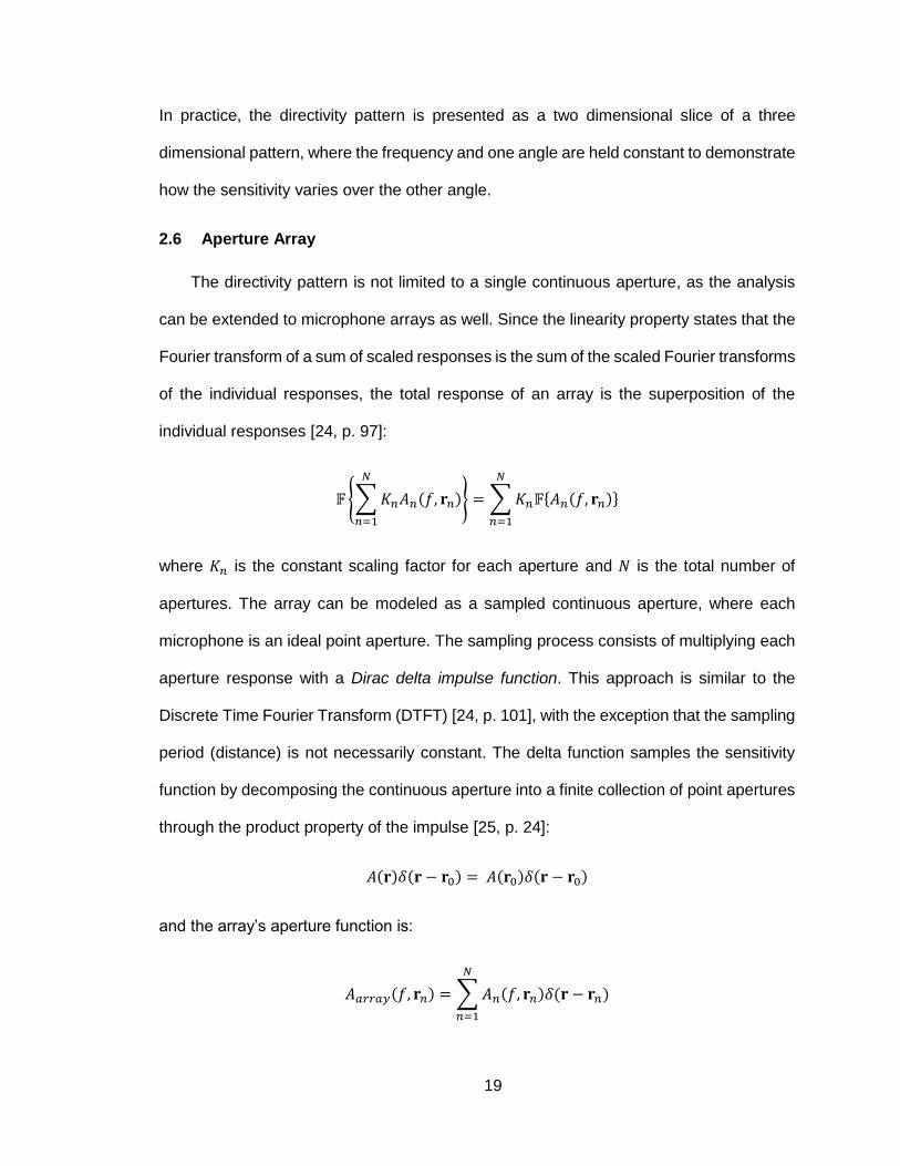
The directivity pattern is not limited to a single continuous aperture, as the analysis
can be extended to microphone arrays as well. Since the linearity property states that the
Fourier transform of a sum of scaled responses is the sum of the scaled Fourier transforms
of the individual responses, the total response of an array is the superposition of the
individual responses [24, p. 97]:
𝔽 {∑𝐾𝑛𝐴𝑛(𝑓, 𝐫𝑛)
𝑁
𝑛=1
} = ∑𝐾𝑛𝔽{𝐴𝑛(𝑓, 𝐫𝑛)}
𝑁
𝑛=1
where 𝐾𝑛 is the constant scaling factor for each aperture and 𝑁 is the total number of
apertures. The array can be modeled as a sampled continuous aperture, where each
microphone is an ideal point aperture. The sampling process consists of multiplying each
aperture response with a Dirac delta impulse function. This approach is similar to the
Discrete Time Fourier Transform (DTFT) [24, p. 101], with the exception that the sampling
period (distance) is not necessarily constant. The delta function samples the sensitivity
function by decomposing the continuous aperture into a finite collection of point apertures
through the product property of the impulse [25, p. 24]:
𝐴(𝐫)𝛿(𝐫 − 𝐫0) = 𝐴(𝐫0)𝛿(𝐫 − 𝐫0)
and the array’s aperture function is:
𝐴𝑎𝑟𝑟𝑎𝑦(𝑓, 𝐫𝑛) = ∑𝐴𝑛(𝑓, 𝐫𝑛)𝛿(𝐫 − 𝐫𝑛)
𝑁
𝑛=1

20
The Fourier transform of a scaled, spatially offset impulse function applies a phase shift
to each aperture but does not alter the magnitude response [24, p. 96]:
𝐴(𝐫0)𝛿(𝐫 − 𝐫0) ⟺ 𝐴(𝐫0)𝑒−𝑗2𝜋𝛂⋅𝐫0
Thus, each sensitivity function is treated as a constant in the Fourier transformed
response, so the array’s directivity pattern is [21, p. 8]:
𝐷𝑎𝑟𝑟𝑎𝑦(𝑓, 𝛂) = ∑𝐴𝑛(𝑓)𝑒−𝑗2𝜋𝛂⋅𝐫𝑛
𝑁
𝑛=1
2.7 Beamforming
The primary advantage of a microphone array, as opposed to a single aperture, is the
ability to electronically steer the directivity pattern. This is accomplished by applying a
complex exponential weight to each microphone [21, p. 19]:
𝑤𝑛(𝑓) = 𝑎𝑛(𝑓)𝑒𝑗𝜑𝑛(𝑓)
where the amplitude 𝑎𝑛(𝑓) alters the shape of the directivity pattern, and the phase 𝜑𝑛(𝑓)
shifts or steers the pattern [21, p. 19]. This is because the inverse Fourier transform of a
complex exponential produces a time delay, which phase aligns the wave fronts arriving
at different elements in the array. Beamforming is the process of determining the weights
in order to steer and focus the beam pattern towards the sound source for maximum
reception [21, p. 19]. The simplest beamforming method is filter-sum beamforming, which
applies a frequency dependent magnitude and phase weight to each element in the array
[21, p. 23]:
𝐷𝑎𝑟𝑟𝑎𝑦(𝑓, 𝛂) = ∑𝑤𝑛(𝑓)𝐴𝑛(𝑓)𝑒−𝑗2𝜋𝛂⋅𝐫𝑛
𝑁
𝑛=1

21
= ∑𝑎𝑛(𝑓)𝐴𝑛(𝑓)𝑒−𝑗2𝜋𝛂⋅𝐫𝑛𝑒𝑗𝜑𝑛(𝑓)
𝑁
𝑛=1
Delay-sum beamforming is a variation of filter-sum beamforming that applies a frequency
dependent phase weight to steer the main lobe and a frequency independent, constant
amplitude weight to normalize the maximum intensity [21, p. 22]:
𝑎𝑛(𝑓) =1
𝑁, 𝜑𝑛(𝑓) = 2𝜋𝛂
′ ⋅ 𝐫𝑛
𝐷𝑎𝑟𝑟𝑎𝑦′ (𝑓, 𝛂) = ∑
1
𝑁𝐴𝑛(𝑓)𝑒
−𝑗2𝜋𝛂⋅𝐫𝑛𝑒𝑗2𝜋𝛂′⋅𝐫𝑛
𝑁
𝑛=1
=1
𝑁∑𝐴𝑛(𝑓)𝑒
−𝑗2𝜋(𝛂−𝛂′)⋅𝐫𝑛
𝑁
𝑛=1
The normalized wavenumber 𝛂 depends on both the DOA and wavelength. In
practice, the speed of sound through human tissue and the frequency of interest are
known while the wavelength is not, so it is convenient to replace wavelength with both
wave speed and frequency using the relationship:
𝜆𝑓 = 𝜈 ⟶ 𝜆 =𝜈
𝑓
Furthermore, the normalized wavenumber can be expressed as the direction vector 𝛃:
𝛂 =𝛃
λ⟶ 𝛃 = [𝑠𝑖𝑛𝜃𝑐𝑜𝑠𝜙 𝑠𝑖𝑛𝜃𝑠𝑖𝑛𝜙 𝑐𝑜𝑠𝜃]
Thus, the final beam steering formula separates environmental assumptions (frequency
and velocity) from the desired beam direction (𝛃 ∝ θ,ϕ) [21, p. 19]:
𝐷𝑎𝑟𝑟𝑎𝑦′ (𝑓, 𝛃) =
1
𝑁∑𝐴𝑛(𝑓)𝑒
−𝑗2𝜋𝜆(𝛃−𝛃′)⋅𝐫𝑛
𝑁
𝑛=1
=1
𝑁∑𝐴𝑛(𝑓)𝑒
−𝑗2𝜋𝑓𝜈(𝛃−𝛃′)⋅𝐫𝑛
𝑁
𝑛=1

22
The directivity pattern, being a Fourier-transformed function, is susceptible to aliasing.
Spatial aliasing is avoided when the spacing between any two sensors is less than half
the wavelength. When the sensor spacing exceeds this limit, directionality is lost because
the directivity pattern’s main lobe is replicated in the side lobes [21, pp. 13-14].
2.8 Simulation Results
The five element stethoscope array constructed in [20] is simulated in MATLAB with
the stethoscope positions in Figure 2-3.
Figure 2-3: Stethoscope positions in the apparatus [beamforming.m].
The stethoscopes are situated so that they lay over the precordial landmarks when the
apparatus is strapped onto the patient’s chest. The stethoscopes comfortably conform to
the chest since each one is placed in a PVC pipe with foam backing. This arrangement
creates a slight z-plane offset which is difficult to measure and varies between patients,
so it is ignored in the simulation.

23
The simulation is run with the script beamforming.m, where the wave velocity is set
to 1,540 meters/sec, which is the average speed of sound through human tissue [26]. The
target azimuthal angle 𝜙 iterates by 𝜋
6 radians through the range 0 to π, and the directivity
pattern is computed for three different frequencies.

24
The first simulation is performed at a frequency of 500 Hz, which is within the typical
murmur range of 125 to 800 Hz but less than the threshold for spatial aliasing. The results
are displayed in Figure 2-4.

25
Figure 2-4: Steering Φ between 0 and π (f = 500 Hz, no spatial aliasing).

26
The second simulation is performed at a frequency of 7 kHz, which is greater than the
typical murmur range but still less than the threshold for spatial aliasing. The results are
displayed in Figure 2-5.

27
Figure 2-5: Steering Φ between 0 and π (f = 7 kHz, no spatial aliasing).
28
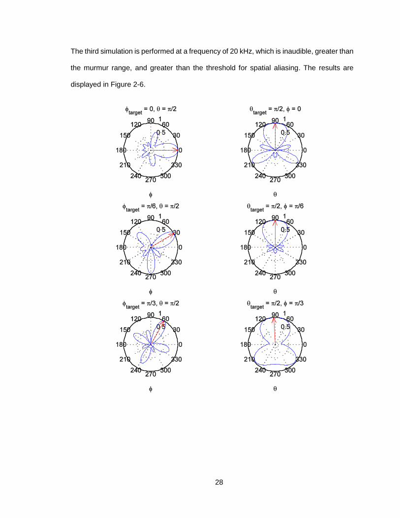
The third simulation is performed at a frequency of 20 kHz, which is inaudible, greater than
the murmur range, and greater than the threshold for spatial aliasing. The results are
displayed in Figure 2-6.

29
Figure 2-6: Steering Φ between 0 and π (f = 20 kHz, spatial aliasing).

30
2.9 Discussion
The simulation at 7 kHz is the most effective of the three frequencies for beamforming
applications. The main lobe (red arrow) is sufficiently narrow and effectively tracks the
target angle, and the wavelength is large enough compared to the sensor spacing to
prevent spatial aliasing. Unfortunately, the frequency is too large for the murmur spectral
range.
The simulation at 20 kHz has the narrowest main lobe at the expense of spatial
aliasing, which duplicates the main lobe at the side lobes. The main lobe nonetheless
accurately tracks the target angle, but like the 7 kHz simulation, the frequency range
exceeds that of the murmur, and is therefore unsuitable for the stethoscope array.
The simulation at 500 Hz has the least directionality of the three simulations. The
directivity pattern is roughly a sphere without a distinguishable main lobe. The maximum
intensity (red arrow) is only slightly greater than the rest of the pattern’s intensity, but it
does manage to track the target angle nonetheless. Additionally, the wavelength is large
enough compared to the sensor spacing that spatial aliasing does not exist. Unfortunately,
the uniformity of the directivity pattern makes this frequency unsuitable for effective beam
steering.
These three simulations show that the main lobe’s width is inversely proportional to
the frequency. However, it is also known that sensor density is inversely proportional to
the main lobe width. Adding more stethoscopes to the array could possibly make
beamforming feasible in the murmur’s frequency range, but the size and constrained
locations of the stethoscopes makes it impractical to add more. Therefore, beamforming
is not a suitable technique for the five element stethoscope array since the frequencies in
the heart murmur range do not produce a narrow enough main lobe to steer the beam
pattern.

31
3 Segmentation Algorithms and Concepts
3.1 Frequency Domain Filtering
The Fourier series maps a periodic, continuous signal to the discrete Fourier
coefficients 𝑐𝑘 located at integer multiples of the fundamental frequency 𝜔0 [24, p. 84]:
𝑐𝑘 =1
𝑇0∫ 𝑥(𝑡)𝑒−𝑗𝑘𝜔0𝑡𝑑𝑡
𝑇0
The Fourier transform 𝔽 maps an aperiodic, continuous signal to the continuous frequency
spectrum 𝑋(𝜔) by evaluating the limit of the Fourier series coefficients as the period
approaches infinity [24, p. 91]:
lim𝑇0→∞
2𝜋
𝑇0= 𝑑𝜔
𝜔0=2𝜋
𝑇0→ lim
𝑇0→∞𝑘𝜔0 = 𝑘𝑑𝜔 = 𝜔
𝑐𝑘∞ = lim𝑇0→∞
1
2𝜋
2𝜋
𝑇0∫ 𝑥(𝑡)𝑒−𝑗𝑘𝜔0𝑡𝑑𝑡
𝑇0
=1
2𝜋[∫ 𝑥(𝑡)𝑒−𝑗𝜔𝑡𝑑𝑡
∞
−∞
] 𝑑𝜔 =1
2𝜋𝑋(𝜔)𝑑𝜔
𝔽{𝑥(𝑡)} ≡ 𝑋(𝜔) = ∫ 𝑥(𝑡)𝑒−𝑗𝜔𝑡𝑑𝑡∞
−∞
The shared connection between the Fourier series and the Fourier transform is that both
use a periodic basis function to quantify the frequency distribution. In practice, it is simpler
to use the Fourier transform for both periodic and aperiodic signals. Instead of integrating
for the Fourier series, periodic signals can be truncated to a single period and transformed
using tables of common transform pairs and properties. Thus, the concepts presented
here apply equally to the Fourier transform and the Fourier series.

32
The utility of the complex exponential basis function is obscured by its notation.
Euler’s identity reveals that the complex exponential is fundamentally sinusoidal [24, p.
84]:
𝑒−𝑗𝜔𝑡 = cos(𝜔𝑡) − 𝑗 sin(𝜔𝑡)
The symbol 𝑗 denotes that the real and imaginary components are separate stores of
information. In fact, sine and cosine are orthogonal functions [24, p. 83]:
∫ cos(𝜔𝑡) sin(𝜔𝑡) 𝑑𝑡 = 0
2𝜋
0
because they are completely uncorrelated, despite only differing by a phase offset. Since
sine and cosine both exist in ℝ2, and addition or subtraction would only superimpose the
two sinusoids, they are instead represented as orthogonal vectors in the complex plane
or ℂ2. Thus, their vector sum is the complex exponential, so that the cosine component
lies on the real axis, the sine component lies on the imaginary axis, and the locus of all
points is the unit circle.
Applying Euler’s identity to the complex exponential demonstrates that the Fourier
transform is a correlation between the input signal and two orthogonal sinusoids [24, p.
603]:
𝑋(𝜔) = ∫ 𝑥(𝑡) cos(𝜔𝑡) 𝑑𝑡∞
−∞
− 𝑗∫ 𝑥(𝑡) sin(𝜔𝑡) 𝑑𝑡∞
−∞
In general, both integrals are necessary for determining the spectrum of any continuous,
physically realizable signal. For example, the sine and cosine Fourier transform pairs are
given as [24, p. 96]:
cos(𝜔0𝑡) ⟷ 𝜋[𝛿(𝜔 − 𝜔0) + 𝛿(𝜔 + 𝜔0)]

33
sin(𝜔0𝑡) ⟷ −𝑗𝜋[𝛿(𝜔 − 𝜔0) − 𝛿(𝜔 + 𝜔0)]
where the Dirac delta function, 𝛿(𝜔 − 𝜔0), is an infinite-magnitude, infinitesimal duration
pulse located at the sinusoid’s frequency 𝜔0. The cosine spectrum is purely real whereas
the sine spectrum is purely imaginary, but a time delayed cosine has both real and
imaginary spectral components [24, pp. 96-97]:
cos(𝜔0𝑡 − 𝑡0) ⟷ 𝜋[𝛿(𝜔 − 𝜔0) + 𝛿(𝜔 + 𝜔0)]𝑒−𝑗𝜔𝑡0
= cos(𝜔𝑡) [𝛿(𝜔 − 𝜔0) + 𝛿(𝜔 + 𝜔0)] − 𝑗 sin(𝜔𝑡) [𝛿(𝜔 − 𝜔0) + 𝛿(𝜔 + 𝜔0)]
Thus, the delayed cosine correlates with both sine and cosine in the time domain.
Ultimately, there are some signals that only require one of the integrals in the Fourier
transform, but in general, continuous signals require both the sine and cosine integrals.
Just as a spectrum can be obtained through Fourier analysis, a signal can be
constructed from a spectrum. Any periodic signal can be represented with its Fourier
series coefficients as [24, p. 84]:
𝑥(𝑡) = ∑ 𝑐𝑘𝑒𝑗𝑘𝜔0𝑡
∞
𝑘=−∞
= 𝑐0 +∑2|𝑐𝑘|cos (𝑘𝜔0𝑡 + 𝜃𝑘)
∞
𝑘=1
The last expression is the combined trigonometric form or polar form of the Fourier series,
and it demonstrates how a periodic signal can be theoretically generated from a
superposition of amplitude weighted and phase shifted sinusoids. This principle can be
extended to aperiodic signals through the inverse Fourier transform 𝔽−1 [24, p. 91]:
𝑐𝑘∞ =1
2𝜋𝑋(𝜔)𝑑𝜔
𝑥(𝑡) = ∑ 𝑐𝑘∞𝑒𝑗𝑘𝜔0𝑡
∞
𝑘=−∞
= ∑ [1
2𝜋𝑋(𝜔)𝑑𝜔] 𝑒𝑗𝑘𝜔0𝑡
∞
𝑘=−∞
=1
2𝜋∑ 𝑋(𝜔)𝑒𝑗𝑘𝜔0𝑡𝑑𝜔
∞
𝑘=−∞

34
𝔽−1{𝑋(𝜔)} ≡ 𝑥(𝑡) =1
2𝜋∫ 𝑋(𝜔)𝑒𝑗𝜔𝑡𝑑𝜔
∞
−∞
Knowing this, it is possible to attenuate undesirable bands of frequencies, such as
murmurs, and then reconstruct a new signal. However, this is only possible when the heart
sound and murmur frequencies do not overlap in the spectrum, but this is not always the
case as can be seen in Figure 3-1. Since the Fourier transform uses a periodic basis
function, it is assumed that the frequencies exist for all time, but PCG’s are non-stationary
signals because the frequency content varies over time.
Figure 3-1: PCG spectrum [PCG_FFT.m].
The Short-Term Fourier Transform (STFT) is a proposed solution because it adds
time resolution to the spectrum by dividing the signal into segments and performing a
separate Fourier transform on each segment [24, p. 606]:
35
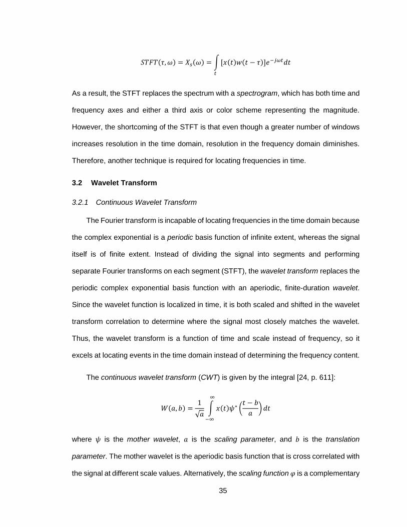
𝑆𝑇𝐹𝑇(𝜏, 𝜔) = 𝑋𝑠(𝜔) = ∫[𝑥(𝑡)𝑤(𝑡 − 𝜏)]𝑒−𝑗𝜔𝑡𝑑𝑡
𝑡
As a result, the STFT replaces the spectrum with a spectrogram, which has both time and
frequency axes and either a third axis or color scheme representing the magnitude.
However, the shortcoming of the STFT is that even though a greater number of windows
increases resolution in the time domain, resolution in the frequency domain diminishes.
Therefore, another technique is required for locating frequencies in time.
3.2 Wavelet Transform
3.2.1 Continuous Wavelet Transform
The Fourier transform is incapable of locating frequencies in the time domain because
the complex exponential is a periodic basis function of infinite extent, whereas the signal
itself is of finite extent. Instead of dividing the signal into segments and performing
separate Fourier transforms on each segment (STFT), the wavelet transform replaces the
periodic complex exponential basis function with an aperiodic, finite-duration wavelet.
Since the wavelet function is localized in time, it is both scaled and shifted in the wavelet
transform correlation to determine where the signal most closely matches the wavelet.
Thus, the wavelet transform is a function of time and scale instead of frequency, so it
excels at locating events in the time domain instead of determining the frequency content.
The continuous wavelet transform (CWT) is given by the integral [24, p. 611]:
𝑊(𝑎, 𝑏) =1
√𝑎∫ 𝑥(𝑡)𝜓∗ (
𝑡 − 𝑏
𝑎)𝑑𝑡
∞
−∞
where 𝜓 is the mother wavelet, 𝑎 is the scaling parameter, and 𝑏 is the translation
parameter. The mother wavelet is the aperiodic basis function that is cross correlated with
the signal at different scale values. Alternatively, the scaling function 𝜑 is a complementary
36
function that can be substituted for the mother wavelet in the integral [24, p. 611]. In fact,
the mother wavelet and the scaling function are equivalent to high-pass and low-pass
filters.
The wavelet transform is typically applied to discrete time signals, which limits the
translation parameter to integer values but does not restrict the scaling parameter.
Therefore, the continuous wavelet transform is so named because the scaling parameter
is continuous, even for discrete time inputs [24, p. 606].
3.2.2 Discrete Wavelet Transform
In contrast to the CWT, the discrete wavelet transform (DWT) does away with the
scaling, translation, and correlation operations and replaces them with the equivalent, but
more efficient, dyadic down sampling and convolution. The mother wavelet and scaling
functions are the same functions from before, except that they are now treated as impulse
responses that are convolved with the signal rather than correlated. As a result, the mother
wavelet is the high pass decomposition filter, and the scaling function is the low pass
decomposition filter.
The high pass decomposition filter is used to transform the input into the detail
coefficients, while the low pass decomposition is used to transform the input into the
approximation coefficients. The approximation and detail coefficients demonstrate how
the time domain features change at different frequency bands or decomposition levels.
The coefficients for the first level are acquired by separately convolving the PCG with the
low pass and high pass decomposition filters and then down sampling each result by a
factor of two to generate the approximation coefficient CA1 (low pass) and the detail
coefficient CD1 (high pass). Down sampling restricts the first level’s frequency range to
half the sampling rate of the PCG. In particular, CA1 represents the lower half of this
frequency range and CD1 represents the upper half of this frequency range. Each

37
additional level is decomposed by repeating this procedure on the current level’s
approximation coefficient so that the final set of coefficients for N levels, ordered from the
lowest to highest frequency range, is CAN followed by CDN through CD1. The
approximation and detail coefficients can then be modified and reconstructed with the high
pass and low pass reconstruction filters, and the two reconstructed waveforms are
combined to generate the filtered output signal.
For heart sound segmentation, the DWT is used to attenuate murmurs so that the
heart sounds can be segmented. This is achieved by determining the appropriate level
(frequency band) where the heart sounds are concentrated, and then applying the low
pass decomposition filter at this level to generate its approximation coefficient.
Reconstructing just the approximation coefficient will generate an output waveform with
attenuated murmurs. After the heart sounds are segmented, the original PCG is used to
segment and classify the murmurs.
3.3 Simplicity Transform
Given that the discrete wavelet transform’s purpose is to attenuate the murmurs
without otherwise altering the PCG, the heart sounds and murmurs require separate
waveforms for segmentation. Therefore, an alternative segmentation technique is
proposed, one which transforms the PCG into a waveform that can be used to segment
both the heart sounds and murmurs. The underlying algorithm is known as the simplicity
transform because the PCG is transformed into a waveform where the values quantify the
simplicity of short segments in the PCG.
3.3.1 Complexity and Simplicity
The Fourier transform produces its sparsest spectrum when the signal is either a
constant or a sinusoid. The transform pair for the constant is:

38
𝐴 ⟷ 2𝜋𝐴𝛿(𝜔)
Likewise, the transform of a sinusoid is a pair of delta functions (from before). Thus, these
are the “simplest” signals because the spectrum only contains a single frequency.
Alternatively, the Fourier transform of the rectangle function is a sine cardinal or sinc
function (Figure 3-2):
rect(t) ⟺ sinc(𝑓) =sin(𝑓)
𝑓
This is the most “complex” signal because its spectrum spans all frequencies.
Consequently, sinusoids and rectangles are not physically realizable because real signals
can neither persist for all time nor span all frequencies. However, both of these limiting
cases demonstrate that “simple” signals have compact spectral ranges while “complex”
signals have broad spectral ranges.
Figure 3-2: Fourier transform of the sinc function [rect_sinc.m].
39
Compared to the irregular shape of murmurs and background noise, heart sound
segments (S1/S2 or S3/S4) resemble simple wavelet packets. Furthermore, auscultation
reveals that murmurs resemble rumbles, clicks, or snaps while heart sounds are simple
beats. Intuitively, heart sounds are “simple” while murmurs and noise are “complex”. Thus,
one way to separate heart sound segments from murmur segments is to calculate the
signal’s simplicity. Since heart sounds are the “simplest” segments in a PCG, the
segments with simplicities greater than a threshold are classified as heart sounds, while
the segments with simplicities less than the threshold are classified as either murmurs or
noise. The inverse of simplicity is the complexity, so depending on the context, either term
may be used to describe a signal. In general, Fourier analysis is unsuitable for quantifying
simplicity, so the preferred method for calculating the simplicity is singular spectrum
analysis.
3.3.2 Dynamical Systems
Dynamical systems theory is the study of how a system’s state changes over time.
The state is represented with state variables, which are elements of the N-dimensional
state vector:
𝐲(𝑡) = [𝑦1, 𝑦2, … , 𝑦𝑛−1, 𝑦𝑛]𝑇
The orbit or trajectory is the time evolution of the state vector in N-dimensional state space
or phase space. The dynamics of the system are the rules that specify a future state from
an initial state, which are specified by the state transition function 𝜙:
𝐲(𝑡) = 𝜙(𝑡, 𝐲(0))
The initial state is time independent, so it can be placed at any position on the trajectory.
Differentiating the state transition function produces a vector field in state space that
assigns a “velocity” to every point on the trajectory [27]:

40
𝑑𝐲(𝑡)
𝑑𝑡= 𝐅(𝐲(𝑡))
An illustrative state space example is the orbit of a planet around the sun. The state
variables are the planet’s position and velocity relative to the Earth, and the state transition
function is Newton’s Law of Gravitation. Prior to discovering solar system dynamics,
namely, the heliocentric model, Kepler’s elliptical orbit theory, and Newton’s Laws, the
planetary positions were geometrically tracked with epicycles [28]. Epicycles accurately
predicted the locations of planets in the sky, but the state variables were hidden because
it was assumed that the sun and the planets orbited Earth; and the state transition function
was unknown because the Law of Gravitation was not yet discovered. Likewise,
auscultation is used to accurately diagnose heart conditions without requiring complete
knowledge of the heart’s state or its underlying dynamics; but unlike epicycles,
auscultation is still the most commonly used form of diagnosis because it is convenient,
inexpensive, and nonintrusive.
3.3.3 The Method of Delays
In general, a measurement can be modeled as a function of a hidden state vector
[13]:
𝑥(𝑡) = ℎ(𝐲(𝑡)) + 𝑤(𝑡)
Here the functional ℎ(𝐲(𝑡)) maps the state vector to a scalar, and 𝑤(𝑡) represents white
noise. Although it is impossible to recover the state vector from a single measurement,
Takens’ embedding theorem states that it is possible to reconstruct the state space
trajectory from a sufficient number of noiseless measurements. The M-dimensional delay
vector [13, p. 1008]:
𝐱𝑖(𝑡) = [𝑥(𝑡), 𝑥(𝑡 − 𝜏),⋯ , 𝑥(𝑡 − (𝑚 − 1)𝜏)]𝑇 (𝑚 > 2𝑛 + 1)

41
is an embedding, or one-to-one mapping, from N-dimensional to M-dimensional state
space [29]. Takens’ theorem proves that the delay vector and the state vector follow similar
dynamics in different state spaces [13, p. 1008]:
𝐱𝑖(𝑡) → 𝐱𝑖(𝑡 + 𝑇) ⟺ 𝐲(𝑡) → 𝐲(𝑡 + 𝑇)
Since a PCG (phonocardiogram) is a discrete time series, the delay 𝜏 is chosen to be the
sampling period so that the delay vector simply contains consecutive samples.
In practice, Takens’ theorem is impractical for reconstructing the signal’s exact
trajectory because measurements are always corrupted with noise. However, signal
complexity is proportional to the dimension, rather than the trajectory, in state space, so
estimating the dimension is sufficient. The “method of delays” is an extension of Takens’
theorem for real signals, but instead of using a single delay vector to reconstruct the
trajectory, it uses the complete set of delay vectors to estimate the dimension. The delay
vector 𝐱𝑖(𝑡) acts as a sliding window that is iteratively stored in a new row of the trajectory
matrix 𝐗 until the window reaches the end of the signal [13, pp. 1008-1009]:
𝐗 =1
√𝑃 [ 𝐱1𝑇
𝐱2𝑇
⋮𝐱𝑃𝑇]
=1
√𝑃 [𝐱𝐼 𝐱𝐼𝐼⋯𝐱𝑀]
=1
√𝑃 [
𝑥(𝑡) 𝑥(𝑡 − 𝜏) ⋯ 𝑥(𝑡 − (𝑚 − 1)𝜏)𝑥(𝑡 − 𝜏) 𝑥(𝑡 − 2𝜏) ⋯ 𝑥(𝑡 − 𝑚𝜏)
⋮ ⋮ ⋱ ⋮𝑥(𝑡 − (𝑝 − 1)𝜏) 𝑥(𝑡 − 𝑝𝜏) ⋯ 𝑥(𝑡 − (𝑝 − 1)𝜏 − (𝑚 − 1)𝜏)
]
The trajectory matrix can be interpreted as either containing P rows of M-dimensional
delay vectors or M columns of P-dimensional delay vectors. The subscripts represent the
number of samples minus one that the delay vector is offset; in particular, the M-
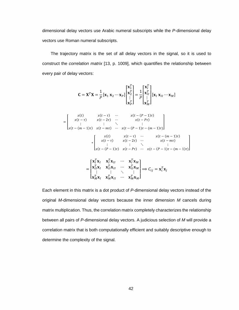
42
dimensional delay vectors use Arabic numeral subscripts while the P-dimensional delay
vectors use Roman numeral subscripts.
The trajectory matrix is the set of all delay vectors in the signal, so it is used to
construct the correlation matrix [13, p. 1009], which quantifies the relationship between
every pair of delay vectors:
𝐂 = 𝐗𝑇𝐗 =1
𝑃[𝐱1 𝐱2⋯𝐱𝑃]
[ 𝐱1𝑇
𝐱2𝑇
⋮𝐱𝑃𝑇]
=1
𝑃[ 𝐱𝐼𝑇
𝐱𝐼𝐼𝑇
⋮𝐱𝑀𝑇 ] [𝐱𝐼 𝐱𝐼𝐼⋯𝐱𝑀]
= [
𝑥(𝑡) 𝑥(𝑡 − 𝜏) ⋯ 𝑥(𝑡 − (𝑃 − 1)𝜏)
𝑥(𝑡 − 𝜏) 𝑥(𝑡 − 2𝜏) ⋯ 𝑥(𝑡 − 𝑃𝜏)
⋮ ⋮ ⋱ ⋮𝑥(𝑡 − (𝑚 − 1)𝜏) 𝑥(𝑡 − 𝑚𝜏) ⋯ 𝑥(𝑡 − (𝑃 − 1)𝜏 − (𝑚 − 1)𝜏)
]
∗ [
𝑥(𝑡) 𝑥(𝑡 − 𝜏) ⋯ 𝑥(𝑡 − (𝑚 − 1)𝜏)
𝑥(𝑡 − 𝜏) 𝑥(𝑡 − 2𝜏) ⋯ 𝑥(𝑡 −𝑚𝜏)
⋮ ⋮ ⋱ ⋮𝑥(𝑡 − (𝑃 − 1)𝜏) 𝑥(𝑡 − 𝑃𝜏) ⋯ 𝑥(𝑡 − (𝑃 − 1)𝜏 − (𝑚 − 1)𝜏)
]
=
[ 𝐱𝐼𝑇𝐱𝐼 𝐱𝐼
𝑇𝐱𝐼𝐼 ⋯ 𝐱𝐼𝑇𝐱𝑀
𝐱𝐼𝐼𝑇 𝐱𝐼 𝐱𝐼𝐼
𝑇 𝐱𝐼𝐼 ⋯ 𝐱𝐼𝐼𝑇 𝐱𝑀
⋮ ⋮ ⋱ ⋮𝐱𝑀𝑇 𝐱𝐼 𝐱𝑀
𝑇 𝐱𝐼𝐼 ⋯ 𝐱𝑀𝑇 𝐱𝑀]
⟹ 𝐶𝑖𝑗 = 𝐱𝑖𝑇𝐱𝑗
Each element in this matrix is a dot product of P-dimensional delay vectors instead of the
original M-dimensional delay vectors because the inner dimension M cancels during
matrix multiplication. Thus, the correlation matrix completely characterizes the relationship
between all pairs of P-dimensional delay vectors. A judicious selection of M will provide a
correlation matrix that is both computationally efficient and suitably descriptive enough to
determine the complexity of the signal.

43
3.3.4 Eigenvalue Decomposition and the Singular Spectrum
In order to determine system complexity, the correlation matrix must be decomposed
into its eigenvalues. The eigenvalues and eigenvectors are given in the equation [13, p.
1009]:
𝐂𝐯 = 𝜆𝐯
where 𝐯 is an eigenvector and 𝜆 is an eigenvalue. The correlation matrix 𝐂 represents a
linear transformation, which can be visualized in three dimensional Euclidean space as a
rotation, reflection, scaling, or shearing. Eigenvectors, by definition, are mutually
orthogonal to each other and maintain the same orientation in space after the linear
transformation. Thus, applying the transformation to an eigenvector is equivalent to
scaling the eigenvector by its eigenvalue. The eigenvalues are found by rearranging the
original equation into the characteristic equation and solving for the roots:
det(𝐂 − 𝜆𝐯) = 0
where the maximum number of eigenvalues is the dimension M of the correlation matrix.
The singular spectrum is the set of eigenvalues stored in a diagonal matrix, ranked by
magnitude in descending order:
𝜆1 > 𝜆2 > ⋯𝜆𝑀⟹ 𝐃 = [
𝜆1 0 0 00 𝜆2 0 00 0 ⋱ 00 0 0 𝜆𝑀
]
A system’s complexity is quantified by the relative magnitude, and total number, of
eigenvalues. A “simple” system contains only a few large-magnitude eigenvalues while a
“complex” system contains many small-magnitude eigenvalues. For example, Figure 3-3
compares the singular spectrum of the sinc function to that of white Gaussian noise
(WGN). WGN is maximally complex, so its spectrum contains the maximum number of

44
eigenvalues with small, comparable magnitudes. However, the sinc function is simple, so
its first eigenvalue’s magnitude is nearly maximized while the few other eigenvalues’
magnitudes are nearly zero.
Figure 3-3: Singular spectra comparison [singular_spectra.m].
3.3.5 Shannon Entropy
The relationship between the singular spectrum and signal complexity mirrors the
relationship between the probability mass function (pmf) of a random experiment and the
uncertainty of the experiment’s outcome. The information content 𝐼 is the number of
symbols required to represent an outcome given a symbol set of size 𝑏 and a sample
space with 𝐾 outcomes. For example, one bit is sufficient to represent the outcome of a
coin flip but not the outcome of a six-sided die roll. The first bit distinguishes two
equiprobable events, such as sides 1-3 and 4-6. A second bit distinguishes side 1 from

45
sides 2-3 and side 4 from sides 5-6. If the roll’s outcome is neither side 1 nor 4, then a
third bit distinguishes side 2 from 3 and side 5 from 6. Thus, the information content is
either two or three bits, depending upon the outcome of the roll.
For an experiment with a uniform probability distribution, the average information
content is determined from the probability of a single outcome:
𝑏𝐼 = 𝐾 =1
𝑃
𝐼 = log𝑏1
𝑃= − log𝑏 𝑃
In general, the minimum entropy 𝐻𝑋 is the expected value of the information content of a
random variable 𝑋 [30, pp. 202-203]:
𝐻𝑋 = 𝐸[(𝐼(𝑋)] = ∑𝑃[𝑋 = 𝑘]𝐼(𝑋 = 𝑘)
𝐾
𝑘=1
= −∑𝑃[𝑋 = 𝑘] log𝑏 𝑃[𝑋 = 𝑘]
𝐾
𝑘=1
In other words, it represents the minimum average number of symbols required to
represent an outcome of the random variable [30, p. 209]. For example, imagine picking
a letter from a random word. The probability of a letter occurring is not the same for every
letter, so assume the probability is 10% for each vowel, 2.5% for each consonant other
than X or Z, and 1.25% for X and 1.25% for Z. Instead of using the first bit to divide the
alphabet into two events of thirteen letters each, it is more informationally efficient to
separate the letters into two equiprobable events. Thus, the first bit distinguishes vowels
from consonants because the probability of picking a vowel is 50% and the probability of
picking a consonant is 50%. Likewise, the second bit divides the vowels and consonants.
The probability of choosing the first ten consonants is 25%, and the probability of choosing
the last eleven consonants is also 25% (owing to the lower probability of X and Z).
However, the five vowels cannot be grouped equiprobably, so the average entropy is

46
greater than the minimum average entropy. This process of subdividing the events
continues until the decision tree ends in the outcomes (letters). The minimum entropy of
the experiment with non-uniform letter probabilities is:
𝐻 = 𝑃𝑉𝐼𝑉 + 𝑃𝐶𝐼𝐶 + 𝑃𝑋𝑍𝐼𝑋𝑍
= −5(0.1) log2(0.1) − 19(0.025) log2(0.025) − 2(0.0125) log2(0.0125) = 4.35 bits
In comparison, the minimum entropy of the same experiment with uniform letter
probabilities is:
𝐻 = − log2(26) = 4.70 bits
Thus, for a given random variable, a uniform pmf indicates maximum entropy while a non-
uniform pmf indicates lower entropy. Likewise, for a given trajectory matrix, a uniform
singular spectrum indicates maximum complexity while a non-uniform singular spectrum
indicates lower complexity. In order to quantify complexity, the eigenvalues are normalized
so that they sum to one and are then substituted for probabilities:
𝑃𝑘[𝑀 = 𝑖] = �̂�𝑖(𝑘) =𝜆𝑖(𝑘)
∑ 𝜆𝑖(𝑘)𝑖
where 𝑘 is the sample location of the window and 𝑀 is the eigenvalue index (the “random
variable”). The eigenvalues are used to calculate the entropy of each window:
𝐻𝑀(𝑘) = −∑𝑃𝑘[𝑀 = 𝑖] log2 𝑃𝑘[𝑀 = 𝑖]
𝑖
= −∑�̂�𝑖(𝑘) log2 �̂�𝑖(𝑘)
𝑖
and the entropy is used to determine the complexity Ω(𝑘), which is the average number
of hidden states in the dynamical system:

47
𝐻𝑀(𝑘) = log2Ω(𝑘) → Ω(𝑘) = 2𝐻𝑀(𝑘)
Finally, the simplicity is the inverse of complexity:
simpl(𝑘) =1
Ω(𝑘)
3.4 Piecewise Constant Denoising
The nonlinear simplicity transform is a fundamental algorithm for the comprehensive
PCG segmentation system implemented and tested in this study. Even though the
simplicity transform is more computationally demanding than conventional linear filters,
such as those that use the Fast Fourier Transform (FFT), it can more effectively separate
different sound signatures.
Ideally, each different sound segment in the simplicity-transformed PCG (S1, S2, etc.)
would be represented by a unique, constant simplicity value or level. Instantaneous
transitions between simplicity levels would then occur at the boundaries between different
sound segments at easily identified jump locations. The transformed PCG would then
resemble a piecewise constant (PWC) or jump sparse signal, composed of only a few
unique constant levels [15, p. 7]. The stratification of the PCG simplicity into distinct levels
in this way enables sound segmentation and classification of the more complex murmurs
and sounds by simple thresholding. However, since the raw simplicity values do not
provide an ideal piecewise constant representation (as seen in Figure 3-4), it is necessary
to first filter the noise in the raw simplicity values before attempting sound segmentation
on the waveform.
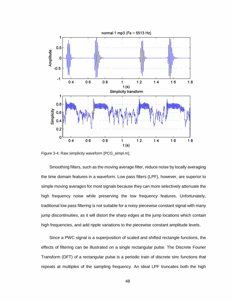
48
Figure 3-4: Raw simplicity waveform [PCG_simpl.m].
Smoothing filters, such as the moving average filter, reduce noise by locally averaging
the time domain features in a waveform. Low pass filters (LPF), however, are superior to
simple moving averages for most signals because they can more selectively attenuate the
high frequency noise while preserving the low frequency features. Unfortunately,
traditional low pass filtering is not suitable for a noisy piecewise constant signal with many
jump discontinuities, as it will distort the sharp edges at the jump locations which contain
high frequencies, and add ripple variations to the piecewise constant amplitude levels.
Since a PWC signal is a superposition of scaled and shifted rectangle functions, the
effects of filtering can be illustrated on a single rectangular pulse. The Discrete Fourier
Transform (DFT) of a rectangular pulse is a periodic train of discrete sinc functions that
repeats at multiples of the sampling frequency. An ideal LPF truncates both the high

49
frequency noise and the high frequency side lobes of the sinc function. After applying the
inverse DFT to the filtered frequency domain representation, the output resembles a PWC
signal, but with ripple throughout, ringing on the edges, and smoothed jumps. This is
similar to the Gibbs phenomenon from the Fourier series, as shown in Figure 3-5. Thus, it
is impossible to recover a noiseless PWC signal using linear frequency domain filtering,
so other noise reduction techniques are required.
Figure 3-5: Low pass filtering a rectangle causes ripple. The signal at the right was filtered with a
higher order LPF than the signal at the left [31].
Piecewise constant denoising or jump sparse reconstruction is the process of
recovering a noisy signal’s optimal PWC representation. It is performed using either level-
set recovery or PWC smoothing algorithms, depending upon the expected number of
unique levels in the recovered signal [15, p. 5]. Level-set recovery uses clustering
algorithms such as K-means or mean shift to separate the sample values into a limited
number of levels, so that the jump locations are found only after the levels are determined
[15, p. 6]. This technique excels at detecting rapid fluctuations between levels, but it is not
suitable for PCG segmentation because heart sound and murmur segments are
associated with a multitude of simplicity levels. PWC smoothing, however, iteratively
estimates a set of jump locations and levels until the output is an optimal PWC
approximation of the original signal [15, p. 6] . Being constrained by both jump locations
and sample values incurs an additional, but justified, computational cost for PWC
smoothing because it enables detection of a greater number of unique levels with greater
accuracy than level-set recovery. For example, the simplicity of an extra heart sound

50
(S3/S4) is only slightly greater than the simplicity of a normal heart sound (S1/S2), and
the simplicity of a murmur is significantly less than that of any heart sound. Since neither
extra heart sounds nor murmurs are guaranteed to exist, the algorithm must determine
the number of levels automatically. However, when the simplicity variance is small, as in
the case of normal and extra heart sounds, samples that should be placed in separate
levels might be combined into one level. Thus, level-set recovery is inadequate for the
segmentation and classification of heart sounds and murmurs.
Solvers are algorithms that minimize functionals [15, p. 7]. A functional transforms a
vector input, which is an element of a vector space, into a scalar output. For jump sparse
reconstruction, the solver minimizes the functional by choosing the optimal set of jump
locations and level values. A multitude of solvers exist for both PWC smoothing and level-
set recovery, but all are special cases of a generalized functional. An illustrative example
of functional minimization is determining the shortest path between two points in Euclidean
space. The path can be represented by an infinite number of curves, but the shortest path
is uniquely represented by a line. The vector field is the set of all possible paths, the vector
input is a single path, and the scalar output is length of the shortest path between the two
points. In general, a functional minimizer is not unique, but the most common PWC solvers
produce a convex set of functional outputs, such that each iteration of the solver
approaches the absolute minimum of the functional.
The simplicity transform of a PCG can be represented as a PWC signal corrupted
with additive noise:
𝐱 = 𝐦+ 𝐞
where 𝑥 is the raw simplicity, 𝑚 is the PWC simplicity, and 𝑒 is the noise. The discrete
functional equation for jump sparse reconstruction is given as:

51
𝐻[𝐦] =∑∑Λ(𝑥𝑖 −𝑚𝑗, 𝑚𝑖 −𝑚𝑗, 𝑥𝑖 − 𝑥𝑗, 𝑖 − 𝑗)
𝑁
𝑗=1
𝑁
𝑖=1
where 𝑥 is the input signal and 𝑚 is the output signal for the current iteration of the solver,
so that the first iteration’s input 𝑥0 is the original signal, the last iteration’s output 𝑚𝑘 is the
final PWC approximation, and all other iterations’ inputs and outputs are intermediate
PWC approximations. The solver iterates until 𝐻[𝑚] reaches an absolute minimum, which
is the only minimum if the functional is convex. The inputs to Λ are the differences:
𝑑 = {
𝑥𝑖 −𝑚𝑗𝑚𝑖 −𝑚𝑗𝑥𝑖 − 𝑥𝑗𝑖 − 𝑗
The first three are value differences because they only apply to sample values while the
last is a sequence difference because it only applies to indices. The two types of functions
in Λ are losses and kernels, both of which are non-negative functions of absolute
difference or distance. Loss functions are typically of the form:
𝐿𝑝(𝑑) = |𝑑|𝑝
where 𝑝 ∈ ℝ. For the specific case 𝑝 = 0, the loss reduces to:
𝐿0(𝑑) = |𝑑|0 = {
1 (𝑑 ≠ 0)
0 (𝑑 = 0)
Kernels are non-negative functions of loss and are classified as either value kernels or
sequence kernels. Value kernels operate on value distances while sequence kernels
operate on sequence distances. Hard kernels restrict the loss to a maximum distance
while soft kernels modify the loss over distance. The hard kernel:
𝐾𝑊1,𝑊2,𝑝(𝑑) = 𝐼(𝑊1 ≤ 𝐿𝑝(𝑑) ≤ 𝑊2) = {1, (T)0, (F)

52
uses the indicator function 𝐼(⋅) to set a hard limit on the acceptable range of losses.
Conversely, the soft kernel uses a non-zero, continuous function to modify the loss:
𝐾𝑝(𝑑) = 𝑓 (𝐿𝑝(𝑑)) ≥ 0
Typically, the soft kernel diminishes in value as the loss increases. The decaying
exponential is a commonly used soft kernel because the loss is relatively unchanged over
a short distance but rapidly approaches zero thereafter:
𝐾𝑝(𝑑) = exp (−𝛽𝐿𝑝(𝑑))
Kernels are further classified as either local (at least one sample value is non-unity) or
global (all sample values are unity).
All terms in Λ are the product of a kernel and a loss. The loss directly contributes to
the functional sum while the kernel modifies or restricts the loss:
Λ = 𝐿𝑝(𝑑)𝐾𝑝(𝑑)
A functional that only contains the regularization term:
Λ =|𝑚𝑖 −𝑚𝑗|
𝑝
𝑝
is minimized when all samples in the output 𝐦 are identical because the global kernel
does not modify or restrict the distance between sample values. Conversely, a functional
that only contains the likelihood term:
Λ =|𝑥𝑖 −𝑚𝑗|
𝑝
𝑝𝐼(𝑖 − 𝑗 = 0) =
|𝑥𝑖 −𝑚𝑖|𝑝
𝑝
is minimized when the final output 𝐦1 is identical to the original input 𝐱0 because the
sequence kernel restricts the input and output samples to identical indices. Neither the
53
regularization nor the likelihood term alone is sufficient for producing a PWC signal, but
the combination of the two terms produces a PWC output:
Λ =|𝑥𝑖 −𝑚𝑖|
𝑝
𝑝+ 𝛾
|𝑚𝑖 −𝑚𝑗|𝑝
𝑝
The regularization parameter 𝛾 balances the tradeoff between data-fidelity (likelihood) and
sparsity (regularization). Sparsity is maximized when the sample values are the same and
minimized when the sample values are unique. Conversely, data-fidelity is maximized
when the output matches the input. The likelihood and regularization terms oppositely
influence the shape of the output, so the solver has to balance both requirements to
minimize the functional and produce an optimal PWC representation.
When 𝛾 is zero, the solver does not attempt to minimize the distance between sample
values. As 𝛾 increases, the regularization term increases its contribution to the functional
sum, which forces the solver to minimize the distance between output value samples. As
𝛾 approaches infinity, all output sample values approach the same value. The constant
value that minimizes the functional, then, is the average value of the original signal:
lim𝛾→∞
Λ =|𝑥𝑖 − 𝑐|
𝑝
𝑝
A judicious choice of 𝛾 will balance the influence of both the likelihood and regularization
terms so that the optimal PWC signal has the appropriate balance of sparsity and data-
fidelity.
3.5 Potts Functional
The Potts functional is suitable for jump sparse reconstruction of the simplicity
waveform because it models the input as a blurred PWC signal corrupted with additive
noise [17, p. 3654]:

54
𝐱 = 𝐚 ∗𝐦 + 𝐞
Like before, 𝐱 is the raw simplicity, 𝐦 is the PWC signal, and 𝐞 is the additive noise. The
blurring is modeled as the convolution of the blur kernel 𝐚 with the PWC signal. The blur
kernel is not typically known a priori but is commonly assumed to be Gaussian:
𝐺(𝑥) =1
√2𝜋𝜎2𝑒−𝑥2
2𝜎2
where 𝜎 is the standard deviation. Alternatively, convolution can be reformulated with
matrix multiplication:
𝐱 = 𝐀𝐦+ 𝐞
Here the blur kernel 𝐚 is converted to the blur matrix 𝐀, which takes the form of a Toeplitz
matrix:
𝐀 =
[ 𝑎0 𝑎−1 𝑎−2 ⋯ ⋯ 𝑎−(𝑛−1)
𝑎1 𝑎0 𝑎−1 ⋱ ⋮𝑎2 𝑎1 ⋱ ⋱ ⋱ ⋮⋮ ⋱ ⋱ ⋱ 𝑎−1 𝑎−2⋮ ⋱ 𝑎1 𝑎0 𝑎−1
𝑎𝑛−1 ⋯ ⋯ 𝑎2 𝑎1 𝑎0 ]
The sums in the original discrete functional equation can removed when the losses and
kernels are expressed as vector operations. The loss function takes the form of a p-norm:
𝐿𝑝≠0(𝐝) = ‖𝐝‖𝑝 = (∑|𝑑𝑖|𝑝
𝑛
𝑖=1
)
1𝑝
𝐿0(𝐝) = ‖𝐝‖0 =∑|𝑑𝑖|0
𝑛
𝑖=1
= |{𝑖: 𝑑𝑖 ≠ 0}|
The 0-norm counts the number of non-zero distances, which is represented by the
cardinality operator (absolute value bars) applied to the set {𝑖: 𝑑𝑖 ≠ 0}.
55
Inverse Potts Minimization (iPotts) is the process of solving the Potts functional to
recover an optimal PWC representation. The Potts functional is given as [17, p. 3654]:
𝐻[𝐦] = 𝛾‖∇𝐱‖0 + ‖𝐀𝐦− 𝐱‖𝑝𝑝
The regularization term’s 0-norm counts the total number of jumps:
∇𝑥 = 𝑥𝑖+1 − 𝑥𝑖
‖∇𝐱‖0 = ∑|𝑥𝑖+1 − 𝑥𝑖|0
𝑁−1
𝑖=1
= |{𝑖: 𝑥𝑖 ≠ 𝑥𝑖+1}|
Instead of penalizing the height of each jump, the 0-norm penalizes all jumps equally so
that the final PWC output is less likely to merge two levels separated by only a small jump
height. The likelihood term reduces to:
‖𝐀𝐦− 𝐱‖𝑝𝑝= ‖𝐛 − 𝐱‖𝑝
𝑝=∑|𝑏𝑖 − 𝑥𝑖|
𝑝
𝑁
𝑖=1
Each iteration attempts to construct an improved PWC approximation 𝐦 of the input 𝐱 by
minimizing the noise, which is the distance between aligned samples of the blurred PWC
approximation and the input.
The MATLAB toolbox Pottslab [32] is used for jump sparse reconstruction in the
segmentation system because it implements an efficient iPotts solver. Furthermore,
Pottslab can solve univariate and multivariate signals, it allows the user to choose the
likelihood term’s p-norm, and it is robust enough to handle signals that have missing
samples. This toolbox’s primary benefit for PCG simplicity denoising is the choice of the
p-norm, since the p-norm determines the noise model.

56
4 Segmentation System Implementation
4.1 System Overview
4.1.1 Introduction
The algorithms and concepts introduced in Chapter 3 are combined in various ways
to create a comprehensive heart sound and murmur segmentation system that is able to
detect and classify normal heart sounds (S1/S2), split heart sounds (M1/T1, A2/P2), extra
heart sounds (S3/S4, summation gallops), and murmurs (systolic/diastolic) from a raw
PCG. The system is implemented in MATLAB (R2013b) for its seamless vector operations
and data visualization, extensive signal processing toolboxes, and object oriented
programming (OOP) support.
The first operation is to load the PCG from the file system and remove any noise with
a wavelet filter. Next, the heart sounds and murmurs are segmented using techniques
specific to the particular segmentation function. The heart sound segments are then
searched for split sound components and are consequently split into two segments are
found. As a prerequisite to heart sound and murmur classification, the heart cycles are
segmented by using the PCG’s autocorrelation waveform to locate the cycle boundaries.
The sound sounds in each heart cycle are then classified and stored in specific arrays
such as S1, S2, systolic murmur, diastolic murmur, etc. Custom data types are provided
for quickly determining the detected conditions and the heart cycles in which they are
located. In addition, the segment arrays can be saved to the filesystem or plotted as color
coded segments according to their sound type on the PCG.
4.1.2 Properties and Methods
Object oriented designs encapsulate, or combine, properties (data) and the methods
(functions) that operate on those properties into a class. In MATLAB, each class has a

57
single class definition file that is stored in the directory @classname. At a minimum, this
file declares all properties and methods but may also set default property values and
define methods. Any methods not fully defined in the class definition file must be
implemented in separate files within the class directory. An object is an instance of a class
and contains property values that define its state. The class constructor method initializes
objects by assigning properties their default values or, for undefined properties, an empty
double array. If additional functionality and arguments are required during object
initialization, a custom constructor can be defined as:
obj = classname(args)
The software system for this project supports two distinct segmentation techniques
that, while unique in implementation, retrieve the PCG waveform file in the same manner,
depend on common parameters, store the results in the same format, and summarize and
display the results identically. In addition, both techniques must be able to save the results
to the file system and define default behaviors after reloading the results into the
workspace. Thus, it is beneficial to encapsulate the system’s functions and data in the
class definition file stethoscope.m, where objects of this class are initialized as:
sscope = stethoscope(folder, file, varargin)
In a class definition file, properties are declared in blocks delimited by the properties
end keywords, and functions are declared in blocks delimited by the methods end
keywords. Attributes, contained in parentheses after the properties or methods keywords,
modify how properties are accessed, altered, and stored, and how functions are accessed:
properties (Attribute1 = value1, Attribute2 = value2, ...) prop1 prop2 ... end

58
methods (Attribute1 = value1, Attribute2 = value2, ...) func1 func2 ... end
The attribute Access is common to both properties and methods. For methods, the
default value public allows any function to call those methods, while the value private only
allows class methods (methods within the class) to call those methods. For properties,
Access is just a shortcut that sets the GetAccess and SetAccess attributes to the same
value, where GetAccess controls which functions can query the property values, and
SetAccess controls which functions can modify the property values i.e. change the object’s
state. The default value for both is public so that any function can read and write property
values. This is not always desirable, as it is often necessary to restrict the ability to change
state, so SetAccess=private only allows class methods to modify property values.
Furthermore, GetAccess=private only allows class methods to query property values, but
this attribute-value pair is not applied to any properties in this system because there is no
requirement for hidden data. Finally, SetAccess=immutable only allows the class
constructor to modify property values so that the values are permanent after object
initialization.
By default, properties are stored in memory when an object is in the workspace and
stored in a file when the object is saved. The attributes Transient and Dependent modify
how properties are stored in both these cases. Transient properties are stored in memory
but are not stored in the filesystem when the object is saved, and Dependent properties
are never stored but instead calculated when accessed because they depend on the
values of other properties. These attributes’ values are logical, so they can either accept
a Boolean value of true or false or are implicitly true when listed without a value.

59
Methods are distinguished from functions by the manner in which they are called and
their type of arguments. Since methods operate on objects, the first and only required
argument to a method is an object of the method’s class. However, static methods, or
methods with the Static attribute, do not require this argument, as they are auxiliary
methods that do not operate on an object of their class and are called as:
class_name.static_method(args)
The static method loadobj() loads object data from a file into an object in the workspace.
Like the class constructor, loadobj() can be optionally defined for custom behavior, but
unlike the constructor, loadobj() cannot be called directly.
The properties in stethoscope.m are classified as either constants or data. Constants
are not literal constant data types, as their values can be changed, but are so named
because the PCG retrieval, wavelet pre-filtering, and segmentation methods reference,
rather than modify, their values. The constants file and folder are required arguments to
the class constructor since they are empty by default, but even constants with non-empty
default values can be changed through additional constructor arguments, namely, optional
arguments and parameters. Optional arguments, if passed, are listed in a predefined order
after the required arguments so that each value is assigned to the correct property.
Parameters, however, may be listed in any order after the required and optional arguments
since they are passed as name-value pairs in the format (‘prop’,val). The constants listed
in Table 4-1 can only be set during initialization (SetAccess = immutable) whereas those
listed in Table 4-2 can be set during and after initialization (SetAccess = public) using the
dot notation sscope.prop=val. In both tables, the constants are grouped and labeled in
accordance with the methods that reference them.

60
In contrast to constant properties, data properties cannot be set directly because they
contain the results generated from class methods (SetAccess = private). These are listed
in Table 4-3, where the properties that contain raw segmentation data are labeled as
Segmentation Data, and the properties that contain data produced from other class
methods or derived from the raw segmentation data are labeled in accordance with their
attributes (either Dependent or Transient).
Table 4-1: stethoscope.m constant properties (SetAccess = immutable).
Properties Type Argument Default Range
PC
G R
etr
ieval
folder char vector required empty NA
file char vector required empty NA
path char vector no empty NA
max_PCG_dur double scalar parameter 5 positive reals
min_PCG_dur double scalar parameter 0 [0,max_PCG_dur)
Fs_min double scalar parameter 4 kHz positive reals
ds_type char vector parameter ‘dyadic’ ‘dyadic’ ‘integer’ ‘none’
Table 4-2: stethoscope.m constant properties (SetAccess = public).
Properties Type Argument Default Range
DW
T
show_filt logical scalar parameter false true, false
wavef char vector parameter ‘db6’ NA
lvl double scalar optional 0 nonnegative integers
Se
gm
en
tati
on
show_results logical scalar parameter false true, false
max_HS_dur double scalar parameter 0.5 s positive reals
min_HS_dur double scalar parameter 20 ms positive reals
min_syst_dur double scalar parameter 100 ms positive reals
min_murm_dur double scalar parameter 20 ms positive reals
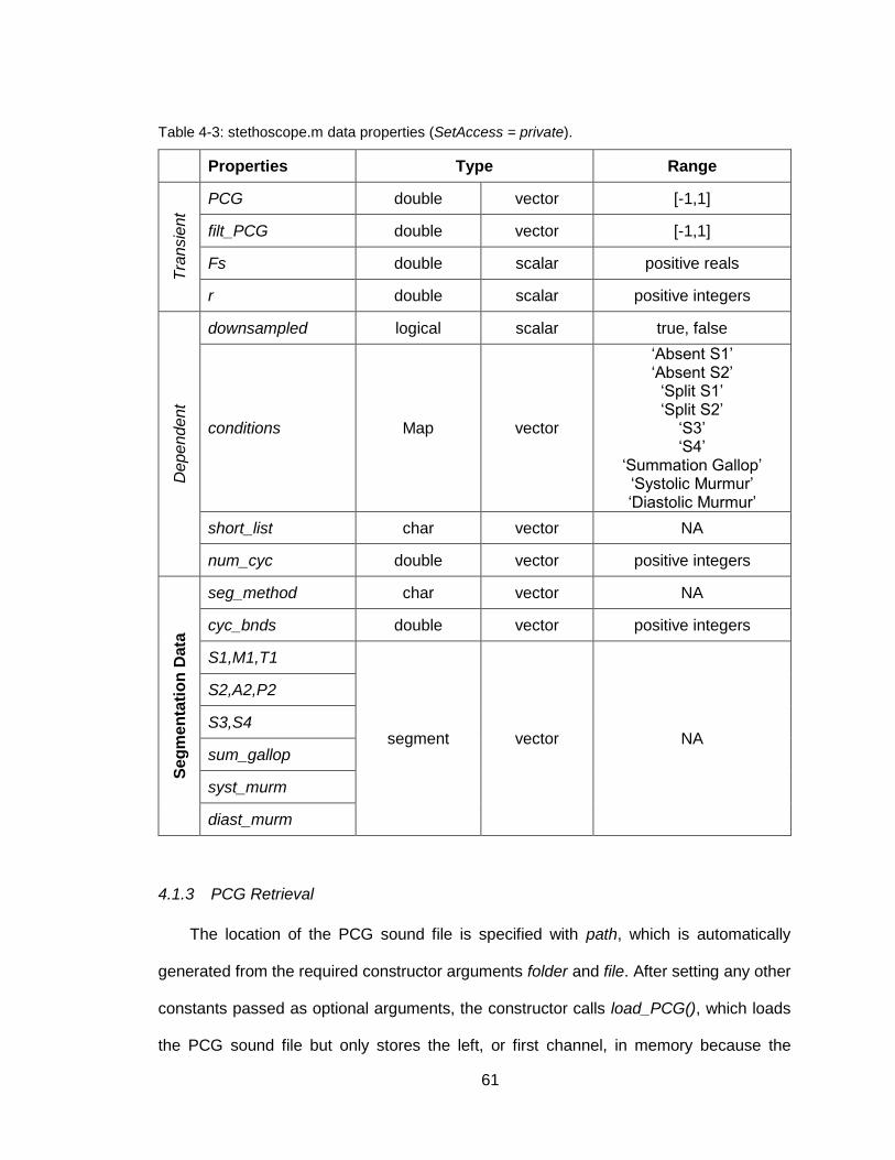
61
Table 4-3: stethoscope.m data properties (SetAccess = private).
Properties Type Range T
ran
sie
nt
PCG double vector [-1,1]
filt_PCG double vector [-1,1]
Fs double scalar positive reals
r double scalar positive integers
De
pe
nd
en
t
downsampled logical scalar true, false
conditions Map vector
‘Absent S1’ ‘Absent S2’
‘Split S1’ ‘Split S2’
‘S3’ ‘S4’
‘Summation Gallop’ ‘Systolic Murmur’ ‘Diastolic Murmur’
short_list char vector NA
num_cyc double vector positive integers
Se
gm
en
tati
on
Data
seg_method char vector NA
cyc_bnds double vector positive integers
S1,M1,T1
segment vector NA
S2,A2,P2
S3,S4
sum_gallop
syst_murm
diast_murm
4.1.3 PCG Retrieval
The location of the PCG sound file is specified with path, which is automatically
generated from the required constructor arguments folder and file. After setting any other
constants passed as optional arguments, the constructor calls load_PCG(), which loads
the PCG sound file but only stores the left, or first channel, in memory because the
62
segmentation functions require a single channel. The min_PCG_dur and max_PCG_dur
constants specify the lower and upper limits, respectively, of the PCG’s duration in
seconds, so the PCG is rejected if its duration is less than the minimum but is simply
truncated if its duration exceeds the maximum. The PCG is also rejected if its sampling
frequency is less than the minimum given by Fs_min. If ds_type (down sampling type) is
either ‘dyadic’ or ‘integer’, load_PCG() calculates a down sampling factor r such that the
down sampled frequency is as close to, but not less than, Fs_min. The default value
‘dyadic’ restricts r to positive powers of two for efficiency while ‘integer’ restricts r to
positive integers. Thus, if r is greater than one, the sampling frequency is reduced by
removing every rth sample. If down sampling is unnecessary, it can be disabled by setting
ds_type to ‘none’.
The results of load_PCG() are stored in PCG, Fs, and r, all of which are Transient
because it is inefficient to save the PCG samples when saving the object to the file system.
Instead, the PCG can be reloaded exactly as before using load_PCG() since the constants
that affect PCG retrieval are immutable and unchanged for the life of the object. Thus,
load_PCG() is the first statement executed upon loading the object from the filesystem
using the custom loadobj().
4.1.4 Wavelet filtering
The Discrete Wavelet Transform (DWT) is used to remove sharp edges and noise
from the PCG before segmentation. The properties wavef and lvl specify the wavelet
function and decomposition level, respectively, to be used during wavelet filtering. The
default wavelet function is ‘db6’ (Daubechies wavelet) because it closely resembles the
morphology of S1 and S2, but the default level is zero so that the system does not attempt
to filter the PCG unless the level is explicitly set. When the level is set to a positive integer,
the function dwt_filt() is called immediately after load_PCG() in the class constructor. The

63
PCG is then “low pass” filtered by convolving the approximation coefficient at level lvl with
the low pass reconstruction filter and storing the result in filt_PCG. Thus, the high
frequency features found in detail coefficients at current or lower levels are not included
in the filtered PCG.
The process of choosing the approximation coefficient for reconstruction is
demonstrated in Figure 4-1. CD1 can be removed because it is almost pure noise and
does not contain any discernible heart sound signatures. The heart sounds begin to
appear in CD2 because the lower end of the CD2 frequency range is 689 Hz. Nonetheless,
CD2 can also be removed because its maximum amplitude is three order of magnitude
less than that of CA2, and the noise is still prevalent. The frequency band for CD3 is within
the range of heart sounds and murmurs, the amplitude is only two orders of magnitude
less than that of CD2, and the noise is small compared to the signal. Thus, the PCG is
reconstructed from CA2 alone, so CD2 and CD1 are removed, and frequencies greater than
689 Hz are excluded from the reconstructed the signal. The original and wavelet filtered
PCG’s are compared in Figure 4-2. This particular PCG contains little noise, but the filter
at least smooths sharp edges, which is a necessary prerequisite for the segmentation
functions.
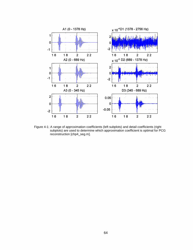
64
Figure 4-1: A range of approximation coefficients (left subplots) and detail coefficients (right
subplots) are used to determine which approximation coefficient is optimal for PCG reconstruction [chp4_seg.m].

65
Figure 4-2: The original PCG (top subplot) has very little noise, so the filtered PCG (bottom
subplot) appears similar to the original PCG [chp4_seg.m].
4.1.5 Segmentation
The segmentation functions require a special class, segment.m, for referencing and
manipulating heart sound and murmur segments. In particular, this class stores the
segment boundaries and provides methods for common segment operations. Objects of
this class are initialized as:
seg = segment(strt, stop, mag)
where the required arguments strt and stop are the segment’s integer start and stop
indices, respectively; and the optional argument mag is a non-zero magnitude assigned
to the segment, which has a default value of one. The constructor verifies that strt does
not exceed stop and that both are positive integers since they reference array indices. In
66
addition to storing segment boundaries, an object of this class can dynamically calculate
the segment’s duration in samples, seg.dur, and generate a vector of the segment’s
indices, seg.rng.
The first group of methods includes those that manipulate segments. The method:
seg = combine(seg, max_dur)
combines adjacent segments within max_dur samples of each other, where max_dur is
an optional argument that has a default value of zero. Additionally, the method:
seg = split(seg, loc)
splits segments apart at the sample locations given in the array loc such that the split
segments are separated by one sample.
The second group of methods includes those that generate a signal from segments.
The method:
sig = mask(seg, sz)
creates a vector of dimension sz that has a value of one for samples within the segment
boundaries and a value of zero for samples outside of the segment boundaries. The
method:
sig = levels(seg, sz)
does the same, except samples within the segment boundaries have a value of seg.mag.
Finally, the method:
sig = signal(seg, ref, zero)
creates a copy of the reference signal ref, but sets samples outside of the segment
boundaries to the value zero. This method is typically used to generate segment layers

67
for a plot, where zero = NaN so that samples between segments do not appear on the
plot.
4.1.6 Storing and summarizing results
The segmentation results are stored in the sscope object in separate arrays named
for the heart sound and murmur types. Six segment arrays are created for the normal
heart sounds (S1, M1, T1, S2, A2, P2) and three for the extra heart sounds (S3, S4,
sum_gallop), where each array has the same number of elements as the number of
detected heart cycles and contains at most one segment per heart cycle. Thus, the
location of non-empty segments in an array indicate which heart cycles contain those
segments, while the locations of empty segments in an array indicate which heart cycles
do not contain those segments. The systolic and diastolic murmur segments are stored in
two cell arrays (syst_murm, diast_murm) of the same length as the heart sound arrays,
and each cell contains a variable length segment array since there can be more than one
murmur segment in either systole or diastole.
Since it is difficult to determine which conditions are detected and in what heart cycle
they are located from the raw heart sound and murmur arrays, stethoscope.m provides
two Dependent properties, sscope.conditions and sscope.short_list, for consolidating and
displaying these results, as well as the class method:
print(sscope)
The first dependent property, conditions, is a map object that extracts the most
relevant information from the arrays. A map links each key in a keyset to a unique value.
In MATLAB, the keys are strings, and the values are objects of a uniform type that are
accessed using the keys as indices:
map_obj(‘key’) = value

68
For conditions, the keys represent the detected heart conditions (Table 4-4), and the
values are numeric arrays that list the number of segments in each heart cycle.
Table 4-4: Set of all possible keys for conditions.
Conditions Keys
Absent S1 as1
Absent S2 as2
Split S1 ss1
Split S2 ss2
S3 s3
S4 s4
Summation Gallop sg
Systolic Murmur sm
Diastolic Murmur dm
The conditions keyset is empty when S1 and S2 are present in each heart cycle because
this is the expected result for a healthy heart. As a result, ‘as1’ or ‘as2’ is only added to
the keyset if an S1 or S2 segment is absent from at least one cycle. Also, ‘ss1’ denotes
the presence of M1 and T1 segments, while ‘ss2’ denotes the presence of A2 and P2
segments. As an example, consider a PCG with four heart cycles and detected absent
S2, split S1, and systolic murmur conditions. The keys and values are listed in Table 4-5.
Table 4-5: Example keys and values for sscope.conditions.
Keys Values
‘as2’ [0 0 0 1]
‘ss1’ [1 1 1 1]
‘sm’ [1 2 2 2]
Here, only the last cycle lacks an S2 segment, all cycles contain one M1 and one T1
segment, and the first cycle contains one systolic murmur while the other three cycles
each contain two systolic murmur segments. Thus, conditions reduces nine segment
arrays and two cell arrays, each of which typically contains many empty elements, into a
single object that specifies the type, quantity, and heart cycle locations of all segments,
which is adequate for diagnosing heart health.
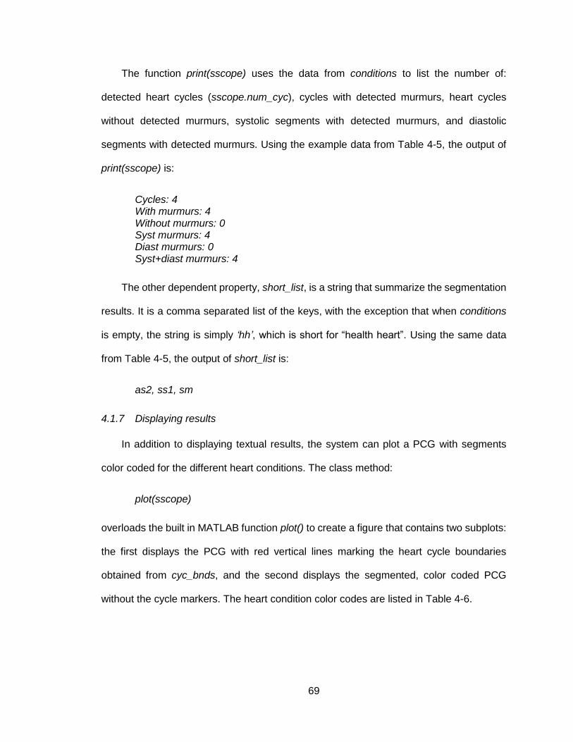
69
The function print(sscope) uses the data from conditions to list the number of:
detected heart cycles (sscope.num_cyc), cycles with detected murmurs, heart cycles
without detected murmurs, systolic segments with detected murmurs, and diastolic
segments with detected murmurs. Using the example data from Table 4-5, the output of
print(sscope) is:
Cycles: 4 With murmurs: 4 Without murmurs: 0 Syst murmurs: 4 Diast murmurs: 0 Syst+diast murmurs: 4
The other dependent property, short_list, is a string that summarize the segmentation
results. It is a comma separated list of the keys, with the exception that when conditions
is empty, the string is simply ‘hh’, which is short for “health heart”. Using the same data
from Table 4-5, the output of short_list is:
as2, ss1, sm
4.1.7 Displaying results
In addition to displaying textual results, the system can plot a PCG with segments
color coded for the different heart conditions. The class method:
plot(sscope)
overloads the built in MATLAB function plot() to create a figure that contains two subplots:
the first displays the PCG with red vertical lines marking the heart cycle boundaries
obtained from cyc_bnds, and the second displays the segmented, color coded PCG
without the cycle markers. The heart condition color codes are listed in Table 4-6.

70
Table 4-6: Heart sound and murmur segment color codes for plot(sscope).
Segments Colors
S1 Blue
S2 Red
S3 Purple
S4 Green
Summation Gallop Black
Systolic Murmur Magenta
Diastolic Murmur Magenta
As an example, a figure with both systolic murmur and split S2 segments can be seen in
Figure 4-3.
Figure 4-3: Graphical segmentation results for a PCG with systolic murmurs and split S2
[chp4_seg.m].

71
4.2 Wavelet-based Segmentation
4.2.1 Heart Sound Segmentation
The two segmentation functions developed for this project are differentiated by the
specific algorithms used to distinguish heart sounds and murmurs, as this is the most
fundamental operation for PCG segmentation. The function:
sscope = dwt_segment(sscope, lvl, varargin)
attenuates the murmur samples using the discrete wavelet transform (DWT), so that the
heart sounds can be segmented. As can be seen in Figure 3-1, the DWT is used in place
of a frequency domain filter because the heart sounds and murmurs often overlap in
frequency but have different time domain morphologies. This function’s wavelet filter, like
the stethoscope object’s wavelet pre-filter, reconstructs a copy of sscope.PCG from its
approximation coefficient at the decomposition level given by lvl. Since heart sounds and
murmurs have lower frequencies than noise and sharp edges, and higher levels represent
lower frequency bands, lvl must be greater than the pre-filter’s level given by sscope.lvl.
The wavelet filter imperfectly attenuates the murmur samples, so any low amplitude
samples must be zeroed through simple thresholding prior to heart sound segmentation.
Since the PCG waveform oscillates between positive and negative values, the threshold
is instead applied to the positive-valued energy waveform, which is typically calculated
using the squared energy function. However, the squared energy function is unsuitable
for thresholding here because it increases the energy separation between medium and
high amplitude inputs significantly since its slope is directly proportional to amplitude. In
contrast, the Shannon energy (SE) is minimized at small and large amplitudes but
maximized at medium amplitudes:
𝑆𝐸(𝑥) = 𝑥2 log 𝑥2

72
This is optimal for thresholding because the medium amplitude heart sounds are
compressed into a smaller energy range, but not attenuated, while the low amplitude
murmurs are assigned a low energy value. This creates an adequate separation between
heart sounds and attenuated murmurs for simple thresholding. The Shannon energy and
squared energy curves are compared in Figure 4-4 to demonstrate how the Shannon
energy is maximized near the medium amplitudes while the squared energy continuously
increases throughout the amplitude range.
Figure 4-4: Shannon energy vs squared energy [energy_functions.m].
In order to prevent high amplitudes from being assigned low energy values less than
the threshold, the Shannon energy waveform is obtained through a sliding window
operation. The window averages the energy over a range of samples to reduce the effect
of large-amplitude spikes in heart sound segments, and it “slides” or advances by one
sample at a time to produce a large overlap that smooths the resulting energy waveform.

73
Two separate thresholding operations are applied to the energy signal to zero the
murmur samples. The first is the peak peeling algorithm adapted from [10], which zeroes
the low energy samples between groups of contiguous higher energy samples, or peaks,
through an iterative thresholding process demonstrated in Figure 4-5. The peak peeling
function:
peaks = peak_peel(x, STC, show, Fs)
begins by applying a standard deviation threshold to the input signal x, and then stores
the results in the peak signal and the rejected signal. The peak signal is a copy of the input
except that sample values less than or equal to the threshold are zeroed (the blue portion
of the waveform in subplot-1). After each iteration, the peak signal is added to a global
output, in which the final output is a sum of all iterations’ peaks (subplot-2). In contrast,
the rejected signal is a copy of the input signal except that sample values greater than the
threshold are zeroed (the red portion of the waveform in subplot-1). The rejected signal,
as its name implies, is not added to the output like the peak signal but is instead the next
iteration’s input. The process only advances to the next iteration if the error, or absolute
difference, between the mean square of the rejected signal and the mean square of the
input signal is greater than the stopping condition given by STC (typically much less than
one). Since the next iteration’s input is always smaller than the current iteration’s input,
the error is reduced after each iteration and approaches the stopping condition. Thus,
peak peeling adaptively determines an appropriate threshold for removing low energy
samples.

74
Figure 4-5: Two peak peeling iterations. Subplot-1 separates the input signal into the peak signal
(blue) and the rejected signal (red). Subplot-2 displays the current output signal, which is a sum of the peaks from the current and previous iterations [chp4_seg.m].

75
The second threshold is a constant rather than an iterative algorithm and, unlike peak
peeling, is applied to the maximum energy of each segment rather than the individual
samples. Thus, the peaks acquired from peak peeling are segmented, and the segments
with maximum energies less than the constant threshold are removed. The murmur
attenuation operations are shown in Figure 4-6, which includes subplots for the PCG,
wavelet reconstructed PCG, and peak peeled Shannon energy. In subplot-3, the segment
that has a maximum energy less than the threshold is removed but nonetheless displayed
on the plot to demonstrate the inadequacies of peak peeling and the necessity of the
constant threshold. In addition to removing low energy segments, segments narrower than
the minimum heart sound segment duration specified by sscope.min_HS_dur are also
removed. The procedure for segmenting heart sounds is summarized in the list below:
1. Calculate the PCG’s Shannon energy waveform
2. Peak peel the Shannon energy
3. Segment the Shannon energy peaks
4. Remove low energy segments
5. Remove short duration segments

76
Figure 4-6: PCG (subplot-1), wavelet reconstructed PCG (subplot-2), and peak peeled Shannon
energy with overlaid constant threshold (subplot-3) [chp4_seg.m].
4.2.2 Removing Murmurs from Heart Sound Segments
As can be seen in subplot-3 of Figure 4-6, incomplete murmur attenuation is
problematic when murmur segments are connected to heart sound segments after peak
peeling. However, there is typically a trough between the connected segments that can
77
be used to reposition the segment boundaries and remove any murmur samples from the
heart sound segments. The local function:
[new_HS, TR_LOC, thresh_lines] = trim_HS(HS, env, rel_thresh)
uses the PCG’s envelope, env, to attempt to find the first trough to the left and to the right
of the heart sound peak within each segment, and then it “trims” the HS segment
boundaries at these trough locations. A heart sound peak is identified because its
amplitude exceeds its containing segment’s threshold given by rel_thresh, which is
specified as a fraction of the segment’s maximum amplitude. For segments containing
multiple heart sound peaks, such as split heart sounds, only the envelope to the left of the
leftmost peak and to the right of the rightmost peak is searched for troughs, so that troughs
between heart sounds are not inadvertently marked. Within trim_HS(), the troughs are
found using the function findpeaks() from the MATLAB signal processing toolbox. The
modified segments are stored in new_HS, the trough locations are stored in TR_LOC, and
information that can be used to plot the threshold lines is stored in thresh_lines.
The segment trimming process is illustrated in subplot-2 of Figure 4-7, where the heart
sound segment boundaries obtained from peak peeling and constant thresholding are
overlaid on the smoothed PCG envelope. The red vertical lines are placed on the segment
boundaries, the horizontal magenta lines represent the peak threshold, and the yellow
markers are placed on the detected trough locations. There are at most two troughs per
segment, but each segment in Figure 4-7 only contains one because the attached
murmurs are located to the right of the heart sounds.
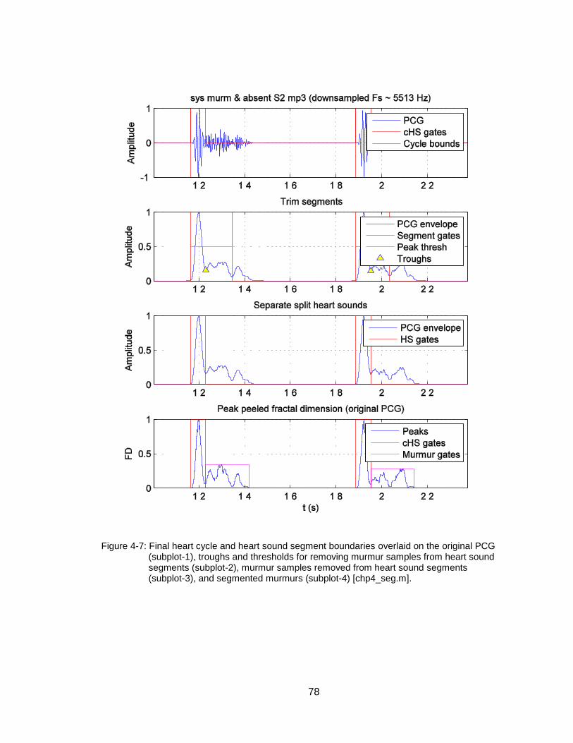
78
Figure 4-7: Final heart cycle and heart sound segment boundaries overlaid on the original PCG
(subplot-1), troughs and thresholds for removing murmur samples from heart sound segments (subplot-2), murmur samples removed from heart sound segments (subplot-3), and segmented murmurs (subplot-4) [chp4_seg.m].
79
4.2.3 Separating Split Heart Sounds
After the heart sound segment boundaries are repositioned so as not to include any
murmur samples, the heart sound segments containing split sounds must be divided into
their split sound components. Split heart sounds are identified when the PCG envelope
has two peaks of a sufficient height within a single heart sound segment. The function:
[HS, TR_LOC, PK_LOC] = split_HS(HS, env, min_dist, min_height)
uses the PCG envelope, env, to find the two largest peaks in each heart sound segment
that are separated by at least min_dist samples (typically set to sscope.min_HS_dur) and
that exceed the magnitude min_height. After the peaks are located, the deepest trough
between the two peaks is located, which is where the heart sound segment is split.
In subplot-2 of Figure 4-8, the split sound components are not marked by trim_HS()
because they lie between two heart sound peaks. For split_HS() In subplot-3, the
horizontal magenta line represents the trough threshold, red markers are placed on the
peaks, yellow markers are placed on the troughs between the peaks, and red vertical lines
denote the new segment boundaries.

80
Figure 4-8: A heart sound segment containing split heart sounds is separated into its component
segments (subplot-3) [chp4_seg.m].
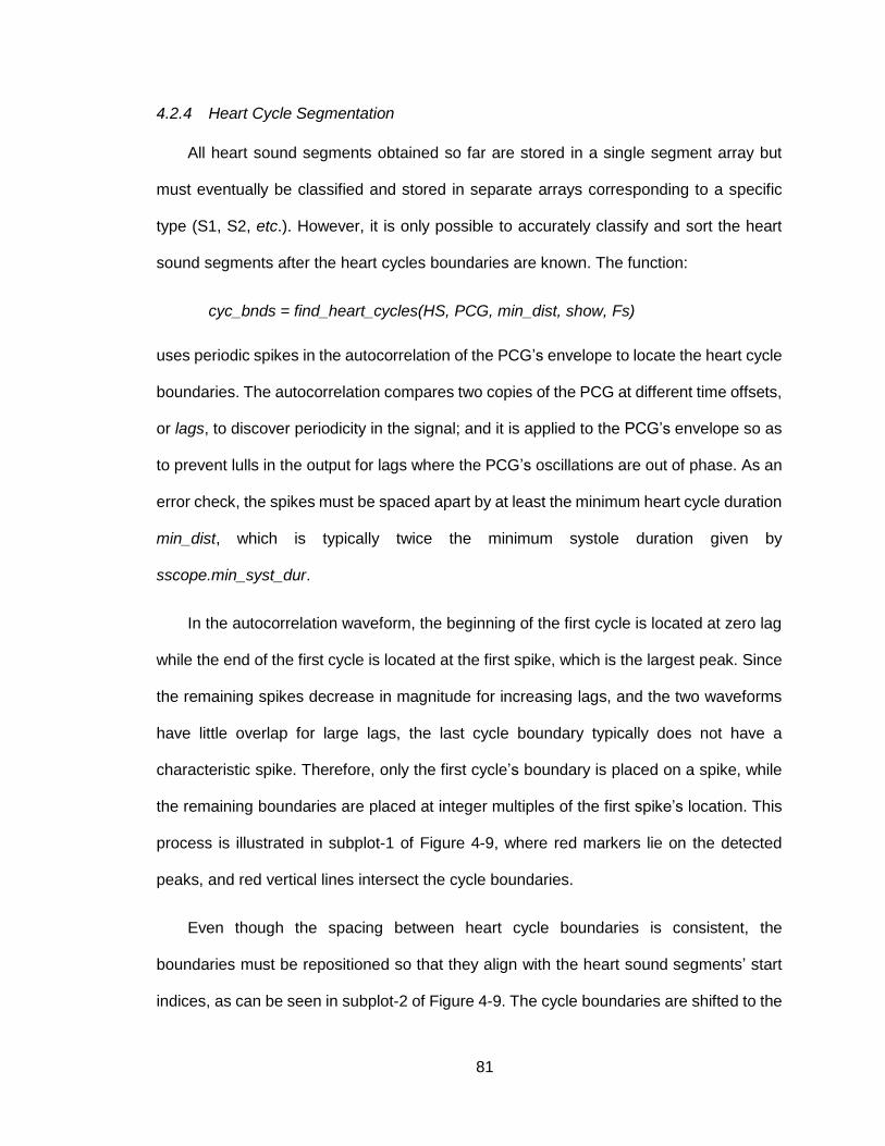
81
4.2.4 Heart Cycle Segmentation
All heart sound segments obtained so far are stored in a single segment array but
must eventually be classified and stored in separate arrays corresponding to a specific
type (S1, S2, etc.). However, it is only possible to accurately classify and sort the heart
sound segments after the heart cycles boundaries are known. The function:
cyc_bnds = find_heart_cycles(HS, PCG, min_dist, show, Fs)
uses periodic spikes in the autocorrelation of the PCG’s envelope to locate the heart cycle
boundaries. The autocorrelation compares two copies of the PCG at different time offsets,
or lags, to discover periodicity in the signal; and it is applied to the PCG’s envelope so as
to prevent lulls in the output for lags where the PCG’s oscillations are out of phase. As an
error check, the spikes must be spaced apart by at least the minimum heart cycle duration
min_dist, which is typically twice the minimum systole duration given by
sscope.min_syst_dur.
In the autocorrelation waveform, the beginning of the first cycle is located at zero lag
while the end of the first cycle is located at the first spike, which is the largest peak. Since
the remaining spikes decrease in magnitude for increasing lags, and the two waveforms
have little overlap for large lags, the last cycle boundary typically does not have a
characteristic spike. Therefore, only the first cycle’s boundary is placed on a spike, while
the remaining boundaries are placed at integer multiples of the first spike’s location. This
process is illustrated in subplot-1 of Figure 4-9, where red markers lie on the detected
peaks, and red vertical lines intersect the cycle boundaries.
Even though the spacing between heart cycle boundaries is consistent, the
boundaries must be repositioned so that they align with the heart sound segments’ start
indices, as can be seen in subplot-2 of Figure 4-9. The cycle boundaries are shifted to the

82
right by a duration equal to the offset of the first heart sound segment because the
autocorrelation waveform only provides information about the relative, rather than the
absolute, cycle boundaries. This shift places the first boundary on the first heart sound
segment’s start index, but the other boundaries do not necessarily lie on heart sound
segment start indices. As a result, these boundaries are moved to the closest segment
start index, and any boundaries shifted beyond the limits of the PCG are removed. To
prevent cycle boundaries from being placed between split heart sound segments,
segments spaced within min_dist samples of each other should be combined prior to
calling find_heart_cycles().

83
Figure 4-9: The heart cycle boundary locations are approximated from spikes in the
autocorrelation of the PCG’s envelope (subplot-1). Afterwards, the cycle boundaries are shifted right and aligned with the nearest heart sound segment start indices (subplot-2) [chp4_seg.m].
4.2.5 Murmur Segmentation
Since the heart sounds serve as the boundaries between which murmurs are
detected, murmurs must be segmented after heart sounds. Murmur segmentation is
similar to heart sound segmentation because a positive-valued waveform is peak peeled
to detect the segment boundaries. However, the fractal dimension of the original PCG,
rather than the energy waveform of the filtered PCG, is peak peeled because the fractal

84
dimension attenuates noise to a greater extent. Thus, subplot-3 in Figure 4-6 is analogous
to subplot-4 in Figure 4-7, as both contain a peak peeled waveform that is used to segment
certain sounds. As with heart sounds, peak peeling is necessary to zero the low intensity
samples in order to extract the sound segment boundaries, but the constant threshold is
unnecessary here because murmurs do not have a minimum required amplitude or
energy. After peeling, the murmur peaks are segmented, and any segments with durations
less than sscope.min_murm_dur are removed.
4.2.6 Heart Sound and Murmur Classification
Only after segmenting the heart sounds, murmurs, and heart cycle boundaries is it
possible to classify and store the segments in separate arrays corresponding to specific
sound types. However, sound segment classification requires that no more than two
normal heart sound segments representing S1 and S2 are present in each heart cycle.
This total does not include split sound segments, as adjacent segments separated by less
than the minimum systole duration (sscope.min_syst_dur) are considered split sound
components and grouped together for the purpose of identifying S1 and S2 segments.
Thus, no more than two normal heart sound segments, or two groups of combined split
sound segments, separated by at least the minimum systole duration may exist in a single
cycle. The function:
[HS, cHS, cyc_bnds] = limit_HS(HS, cHS, cyc_bnds, E)
discards any normal heart sound segments other than the two in each cycle that have the
greatest maximum energy by referencing the energy waveform E. The HS segment array
may contain split sounds since those are combined in the cHS array. Also, if the start index
of a discarded segment lied on a heart cycle boundary, this function will shift the cycle
boundary to the next segment’s start index. Limiting each heart cycle to no more than two
normal heart sound segments is essential for identifying systole and diastole, which are

85
used to classify systolic and diastolic murmurs as well as the extra heart sounds S3, S4,
and summation gallops.
After removing the excess heart sound segments, the function:
[S1, M1, T1, … S2, A2, P2, … S3, S4, sum_gallop, … syst_murm, diast_murm] = lbl_sounds(HS, cHS, cyc_bnds, extra_HS, murm)
classifies the normal heart sounds, extra heart sounds, and murmurs; and transfers
segments from the input arrays HS, extra_HS, and murm to the output arrays that
correspond to specific sounds. Classification operates on a single heart cycle at a time
because the process is dependent on the total number of normal heart sound segments
in each heart cycle. When a cycle contains two normal heart sound segments, the duration
between the stop index of the first segment and start index of the second segment is
compared to the duration between the stop index of the second segment and the end of
the heart cycle. Since these two durations represent either systole or diastole, the shorter
duration is systole and the longer duration is diastole. If both durations are the same, the
first is assumed to be systole and the second is assumed to be diastole. The normal heart
sound segments can therefore be identified because S1 precedes systole and S2
precedes diastole. When a cycle only contains one normal heart sound segment, the
segment is assumed to be S1, and the duration between the S1 stop index and the end
of the heart cycle is assumed to be diastole.
After identifying the S1 and S2 segments, the local function:
[C1, C2] = lbl_split(HS, S)
searches for split sound segments within the boundaries of a heart sound segment (S). If
two segments are found, then the first is stored in C1 and the second is stored in C2; if S

86
does not contain two segments, then C1 and C2 are uninitialized segments. This function
searches S1 for M1 and T1 and S2 for A2 and P2:
[M1, T1] = lbl_split(HS, S1) [A2, P2] = lbl_split(HS, S2)
The systole and diastole segments are then used to classify the murmur segments.
The local function:
murm_type = lbl_murm(murm, sil)
searches for murmur segments within the boundaries of a silent segment (sil), and
recovered murmur segments are stored in the variable length segment array murm_type.
This function searches for both systolic and diastolic murmurs:
syst_murm = lbl_murm(murm, syst) diast_murm = lbl_murm(murm, diast)
Finally, the extra heart sound segments are classified by their locations in diastole.
The local function:
[S3, S4, sum_gallop] = lbl_extra(extra, diast)
searches for extra heart sound segments within the boundaries of a diastole segment
(diast). The murmur segments are classified by their locations relative to the center of
diastole; in particular, S3 segments are located to the left of center, and S4 segments are
located to the right of center. Summation gallops, being the superposition of S3 and S4,
contain the center of diastole within their segment boundaries. In order to prevent
erroneous detection, the number of segments in diastole limits sound classification
behavior. When one segment is present in diastole, it may be classified as either an S3,
an S4, or a summation gallop. When two segments are present, the first segment is S3,
and the second segment is S4. If neither of these configurations are detected, an empty
array is returned rather than an error.

87
Unfortunately, dwt_segment() does not possess the ability to distinguish normal heart
sounds from extra heart sounds, so the extra segment array passed to lbl_sounds() will
be empty. Nonetheless, lbl_extra() is described here because it is a general technique
that is also used in simplicity-based segmentation, as its inputs are segment arrays and
cycle boundaries instead of implementation-specific waveforms
4.3 Simplicity-based Segmentation
The function:
sscope = simpl_segment(sscope, varargin)
utilizes the simplicity transform to segment heart sounds and murmurs as an alternative
to wavelet-based segmentation. Many of the methods and concepts from wavelet-based
segmentation are reused, but new techniques are developed as well. However, the
primary factor that distinguishes simplicity from wavelet-based segmentation is that the
heart sounds and murmurs are segmented in a single operation, which reduces overall
complexity and improves the accuracy of the segment boundaries.
4.3.1 Simplicity Waveform Filtering
An ideal piecewise constant (PWC) function is composed of a series of constant levels
separated by instantaneous transitions at the jump locations. For the simplicity waveform,
the segment boundaries are located at the jump locations, and the value of each
segment’s constant simplicity level distinguishes heart sounds from murmurs.
Unfortunately, the raw simplicity waveform acquired from sscope.filt_PCG is only an
approximate PWC function that must be modified before it can be segmented in this way.
This non-ideal behavior is primarily due to the intrinsic simplicity variation within sound
segments but is also a result of the ripple generated from the sliding window that is used
to obtain the waveform. Furthermore, the raw simplicity values in the silent segments or

88
non-sound segments is often comparable to, or greater than, the simplicity values in the
heart sound and murmur segments. This is a result of sscope.filt_PCG being
reconstructed from a high level approximation coefficient (low frequency band), which has
the effect of both attenuating and smoothing high frequency noise. Since the silent
segments do not contain discernible sounds, the attenuated noise is the primary
determinant of the simplicity in these segments. Even though the smoothing effect on the
noise is hardly noticeable after filtering, the simplicity within the silent segments is
nonetheless high because simplicity is amplitude-invariant (subplot-3 of Figure 4-10).
Therefore, the simplicity within the non-sound segments is set to zero by peak peeling the
PCG’s fractal dimension and then zeroing the same samples in the simplicity waveform
that are zero in the peak peeled fractal dimension (subplot-4 of Figure 4-10). This is similar
to wavelet-based segmentation except that a second, constant threshold for removing low
energy segments is unnecessary here. For efficiency, it is possible to avoid the zeroing
operation (and therefore subplot-3) by only computing the simplicity waveform within the
boundaries of the peaks acquired from peak peeling. The only reason this is not
implemented here is to illustrate the non-ideal behavior of the simplicity waveform outside
of the sound segments.
4.3.2 Piecewise Constant Approximation
After zeroing the silent segments’ simplicity, the simplicity waveform must be
converted to an ideal PWC function. For segments that only contain one sound, the
average simplicity is sufficient for determining the simplicity level; but for segments that
contain multiple sounds, a PWC approximation is required to determine the optimal jump
locations and levels for each sound. Since this is a computationally intensive operation,
and the non-sound segments have zero-value levels, a separate PWC approximation is
performed on each segment rather than the entire waveform (subplot-5 of Figure 4-10).

89
The L2 Potts minimization function from the MATLAB Pottslab toolbox is used to
determine the optimal PWC approximation:
PWC = minL2Potts(signal, gamma)
The gamma constant here is proportional to the output’s coarseness, where a small
gamma closely tracks the input signal, and a large gamma ignores small deviations. The
simplicity waveform’s PWC approximation can be seen in subplot-5 of Figure 4-10, where
the S1, S2, and the holosystolic murmurs that were merged in a single segment even after
peak peeling (subplot-2) can now be individually segmented using the levels and jump
locations in the PWC approximation. The steps required for transforming the raw simplicity
waveform into an ideal PWC function are summarized below:
1. Calculate the PCG’s fractal dimension
2. Peak peel the fractal dimension
3. Calculate the PCG’s simplicity
4. Zero the simplicity in the silent segments
5. PWC approximate the simplicity within each segment

90
Figure 4-10: The peak peeled fractal dimension extracts the sound peaks from the background
noise (subplot-2), which are used to zero the non-sound segments in the raw simplicity waveform (subplot-4) [chp4_seg.m].

91
4.3.3 Heart Sound and Murmur Segmentation
After obtaining the simplicity waveform’s optimal PWC representation, the function:
seg = levels2seg(PWC)
generates a segment for each constant level situated between two jump locations, so that
normal heart sounds, extra heart sounds, and murmurs can be identified by simple
thresholding. The first threshold separates murmurs and heart sounds because murmurs
have lower simplicity due to their complex and irregular shape, whereas heart sounds
have higher simplicity due to their sinusoidal shape. Thus, unlike wavelet-based
segmentation, heart sounds and murmurs are segmented here with a single waveform;
and since the jump locations are the optimal segment boundaries, trim_HS() is not needed
for removing murmur pieces from heart sounds. The second threshold separates normal
and extra heart sounds, which is typically difficult through auscultation alone because both
of these sound types are similar. Furthermore, extra heart sounds are often soft enough
to be inaudible. As a result, the simplicity allows for the extra heart sounds S3, S4, and
summation gallops to be properly identified when their simplicity levels are greater than
those of normal heart sounds (including split sounds). In contrast, wavelet-based
segmentation is incapable of distinguishing normal and extra heart sounds. Both
thresholding operations can be seen in subplot-2 of Figure 4-11.
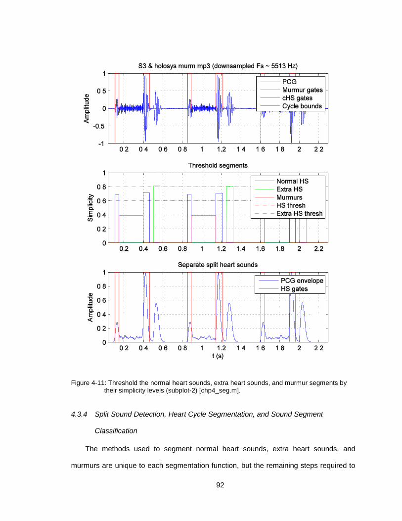
92
Figure 4-11: Threshold the normal heart sounds, extra heart sounds, and murmur segments by
their simplicity levels (subplot-2) [chp4_seg.m].
4.3.4 Split Sound Detection, Heart Cycle Segmentation, and Sound Segment
Classification
The methods used to segment normal heart sounds, extra heart sounds, and
murmurs are unique to each segmentation function, but the remaining steps required to

93
fully classify the segments are nearly identical regardless of the chosen technique. The
first of these is separating heart sound segments that contain split sounds by applying
split_HS() to the PCG’s envelope. The heart cycle boundaries are then obtained with
find_heart_cycles(), and the normal heart sound segments (excluding split sounds) are
restricted to two segments per cycle with limit_HS(). Finally, the normal heart sounds,
extra heart sounds, and murmurs are classified and stored in segments arrays
corresponding to specific sound types with lbl_sounds().

94
5 Segmentation Results
5.1 Introduction
5.1.1 Sound File Datasets
The sound files used for testing the segmentation functions are taken from two
common auscultation training datasets: the Littmann [33] and the University of Michigan
[34] heart sound libraries.
5.1.2 Segmentation Errors and Detection Rates
The primary purpose of PCG segmentation is to detect murmurs because their
presence indicates an unhealthy heart. Normal heart sounds must also be detected
because they are used to locate the heart cycle boundaries and to classify the sound
segment types within each heart cycle. Thus, faulty segmentation is primarily caused by
the incorrect detection of normal heart sounds and murmurs. In particular, this can occur
when heart sounds are misidentified as murmurs and vice versa, or when heart sounds
and murmurs are not detected at all. The detection of split heart sounds and extra heart
sounds is also desirable but not an absolute requirement for diagnosing heart health, as
it is often challenging even through auscultation to distinguish extra sounds from split
sound components. Therefore, successful segmentation here only requires the proper
detection of normal heart sounds and murmurs.
The performance of the wavelet and simplicity-based segmentation methods, as it
relates to medical diagnosis, is evaluated with the false negative detection rate (FNDR)
and the false positive detection rate (FPDR). A false negative occurs when no murmurs
are detected in a murmur-containing heart cycle, which is typically caused by murmurs
being misidentified as heart sounds (false heart sounds). Conversely, a false positive
occurs when a murmur is detected in a murmur-free heart cycle, which is caused by a

95
heart sound being misidentified as a murmur (false murmur). The false negative and false
positive detection rates are defined below:
FNDR = # of murmur-containing heart cycles without detected murmurs / total # of
murmur-containing heart cycles
FPDR = # of murmur-free heart cycles with detected false murmurs / total # of
murmur-free heart cycles
These two metrics indicate the effectiveness of murmur detection by the two
segmentation methods when considering a complete heart sound cycle (composed of one
systole and one diastole segment) as the fundamental unit in which murmurs should be
detected if present. This is similar to when a medical clinician evaluates heart function
during auscultation, as the primary focus is on determining whether or not a murmur is
detected in each heart cycle.
The FNDR and FPDR are sufficient statistics for clinicians, but the true murmur
detection rate (TMDR) and false murmur detection rate (FMDR) are also necessary to fully
evaluate the performance of the two methods. These rates are defined below:
TMDR = # of detected true murmurs / total # of murmurs
FMDR = # of heart cycles with detected false murmurs / total # of heart cycles
For the TMDR, the murmurs are defined as either murmur-containing systole or diastole
segments, so even multiple murmur segments within a systole or diastole segment are
counted as a single murmur. Therefore, the true murmurs are defined as the number of
properly detected and classified murmur-containing systole or diastole segments rather
than individual murmur segments. For the FMDR, the heart cycles include both the

96
murmur-free and murmur-containing heart cycles, so it is a more general rate than the
FPDR, which only considers the murmur-free heart cycles.
Even though the TMDR and FNDR have different evaluative purposes, they are
inversely related. This is because an increase in the number of detected true murmurs
tends to decrease the number of false negative heart cycles. For example, if each heart
cycle contains a systolic murmur, then each additional detected systolic murmur increases
the TMDR and decreases the FNDR.
The underlying causes for the false positives, false negatives, and false murmurs are
discussed and illustrated with examples in sections 5.2 and 5.3.
5.1.3 False Negative and False Positive Detection Rates
The dataset sound files are separated into those that do and do not contain murmurs.
Since false negatives can only occur in murmur-containing cycles, and false positives can
only occur in murmur-free cycles, the FNDR only applies to the sound files that contain
murmurs, and the FPDR only applies to the sound files that do not contain murmurs.
For both wavelet and simplicity-based segmentation, the false negatives are
enumerated in Table 5-1 (Michigan) and Table 5-3 (Littmann), and the false positives are
enumerated in Table 5-2 (Michigan) and Table 5-4 (Littmann). All heart cycles in the false
negative tables contain murmurs, while none of the heart cycles in the false positive tables
contain murmurs. The false negative and false positive data is then used to determine the
FNDR in Table 5-5 and the FPDR in Table 5-6, and both of these detection rates are
compared in Table 5-7.
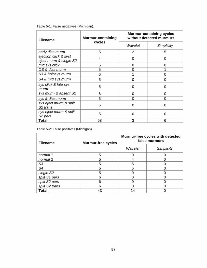
97
Table 5-1: False negatives (Michigan).
Filename Murmur-containing
cycles
Murmur-containing cycles without detected murmurs
Wavelet Simplicity
early dias murm 5 2 5
ejection click & syst eject murm & single S2
4 0 0
mid sys click 5 0 0
OS & dias murm 5 0 1
S3 & holosys murm 6 1 0
S4 & mid sys murm 5 0 0
sys click & late sys murm
5 0 0
sys murm & absent S2 6 0 0
sys & dias murm 6 0 0
sys eject murm & split S2 trans
6 0 0
sys eject murm & split S2 pers
5 0 0
Total 58 3 6
Table 5-2: False positives (Michigan).
Filename Murmur-free cycles
Murmur-free cycles with detected false murmurs
Wavelet Simplicity
normal 1 5 0 0
normal 2 5 4 0
S3 5 5 0
S4 5 5 0
single S2 5 0 0
split S1 pers 6 0 0
split S2 pers 6 0 0
split S2 trans 6 0 0
Total 43 14 0

98
Table 5-3: False negatives (Littmann).
File Name Murmur-containing
cycles
Murmur-containing cycles without detected murmurs
Wavelet Simplicity
AP 0 0 0
AR 4 0 0
AS 3 0 0
ASD 2 0 0
COA 2 0 0
EA 3 0 0
eject click 2 0 0
eject click & AS moderate & AR mild
2 0 0
innocent murmur 2 0 0
late sys click 4 0 0
mid sys click 3 0 0
MR severe 2 0 0
MS moderate 3 1 3
MVP 4 0 0
OS 2 0 0
PDA 2 0 0
S4 & AS severe 2 0 0
TR severe 2 0 0
VSD 2 0 0
Total 46 1 3
Table 5-4: False positives (Littmann).
Filename Murmur-free cycles
Murmur-free cycles with detected false murmurs
Wavelet Simplicity
normal 2 0 0
S3 & S4 3 0 0
S3 abnormal 3 0 0
S3 physio 2 0 0
S4 2 0 0
sum gallop 6 2 0
split S2 fixed 4 0 0
split S2 physio 4 0 0
split S1 4 0 0
Total 30 2 0

99
Table 5-5: False negative detection rates (FNDR).
Dataset Murmur-
containing cycles
Murmur-containing cycles without
detected murmurs FNDR
Wavelet Simplicity Wavelet Simplicity
Michigan 58 3 6 5% 10%
Littmann 46 1 3 2% 7%
Total 104 4 9 4% 9%
Table 5-6: False positive detection rates (FPDR).
Dataset Murmur-free
Cycles
Murmur-free cycles with detected false
murmurs FPDR
Wavelet Simplicity Wavelet Simplicity
Michigan 43 14 0 33% 0%
Littmann 30 2 0 7% 0%
Total 73 16 0 22% 0%
Table 5-7: FNDR and FPDR comparison for wavelet and simplicity-based segmentation.
Technique FNDR FPDR
Wavelet 4% 22%
Simplicity 9% 0%
5.2 Wavelet-Based Segmentation
5.2.1 Wavelet Constants
The constants for wavelet-based segmentation, which consist of window lengths,
peak peeling stopping conditions, thresholds, and wavelet filter-specific values, are listed
in Table 5-8. All constants can be changed from their defaults using name-value pair
arguments passed to dwt_segment() (except for lvl, which is an optional positional
argument). Also, the HS_thresh constant has two values listed for each dataset: 0.1 for
the Michigan dataset (default value) and 0.05 for the Littmann dataset.
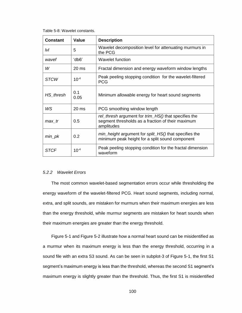
100
Table 5-8: Wavelet constants.
Constant Value Description
lvl 5 Wavelet decomposition level for attenuating murmurs in the PCG
wavef ‘db6’ Wavelet function
W 20 ms Fractal dimension and energy waveform window lengths
STCW 10-4 Peak peeling stopping condition for the wavelet-filtered PCG
HS_thresh 0.1 0.05
Minimum allowable energy for heart sound segments
WS 20 ms PCG smoothing window length
max_tr 0.5 rel_thresh argument for trim_HS() that specifies the segment thresholds as a fraction of their maximum amplitudes
min_pk 0.2 min_height argument for split_HS() that specifies the minimum peak height for a split sound component
STCF 10-4 Peak peeling stopping condition for the fractal dimension waveform
5.2.2 Wavelet Errors
The most common wavelet-based segmentation errors occur while thresholding the
energy waveform of the wavelet-filtered PCG. Heart sound segments, including normal,
extra, and split sounds, are mistaken for murmurs when their maximum energies are less
than the energy threshold, while murmur segments are mistaken for heart sounds when
their maximum energies are greater than the energy threshold.
Figure 5-1 and Figure 5-2 illustrate how a normal heart sound can be misidentified as
a murmur when its maximum energy is less than the energy threshold, occurring in a
sound file with an extra S3 sound. As can be seen in subplot-3 of Figure 5-1, the first S1
segment’s maximum energy is less than the threshold, whereas the second S1 segment’s
maximum energy is slightly greater than the threshold. Thus, the first S1 is misidentified

101
as a murmur, but the second S1 is properly identified (subplot-4 of Figure 5-2). As a result,
the first heart cycle’s start boundary is placed on the start index of the S2 instead of the
S1 segment, which shortens the heart cycle’s duration, removes the systolic murmur from
the heart cycle, and causes S2 to be erroneously classified as S1 (subplot-1 of Figure
5-2). In addition, the S2 and S3 segments in both cycles are misidentified as split
components due to their close proximities and the lack of extra heart sound discrimination
for wavelet-based segmentation. In particular, the S2 and S3 segments in the first cycle
are considered split S1 components, but the S2 and S3 segments in the second cycle are
more appropriately considered split S2 components. Classifying extra heart sounds as
split components is not considered an error per se because the extra sounds resemble
split sounds and are typically located near S1 or S2. Therefore, only a split S2 is detected
in the first cycle as opposed to the S1, systolic murmur, and split S2 detected in the second
cycle.

102
Figure 5-1: The first S1 is mistaken for a murmur because its maximum energy is less than the
energy threshold (subplot-3) [dwt_michigan.m].

103
Figure 5-2: The first S1 segment is misidentified as a murmur, but the second S1 segment is
properly identified (subplot-4). As a result, the first heart cycle’s start boundary is moved from S1 to the nearest S2 (subplot-1) [dwt_michigan.m].

104
Figure 5-3 and Figure 5-4 illustrate how an S4 segment can be misidentified as a
murmur when its maximum energy is less than the heart sound threshold. As can be seen
in subplot-3 of Figure 5-3, similar to the previous example, the first S4 segment’s maximum
energy is less than the threshold, while the second S4 segment’s maximum energy is
greater than the threshold. As a result, the first S4 is misidentified as a murmur, but the
second S4 is acceptably classified as a split S1 component give its proximity to S1
(subplot-4 of Figure 5-4). However, unlike the previous example, the cycle boundaries
here are correctly located since neither S1 nor S2 is removed during segmentation
(subplot-1 of Figure 5-4).

105
Figure 5-3: The first S4 is misidentified as a murmur because its maximum energy is less than the
energy threshold (subplot-3) [dwt_littmann.m].

106
Figure 5-4: The first S4 is misidentified as a murmur, but the second S4 is acceptably
misidentified as a split sound component (subplot-4). The cycle boundary locations are correct because S1 and S2 are properly identified (subplot-1) [dwt_littmann.m].

107
Figure 5-5 illustrates how a murmur can be misidentified as a heart sound when its
maximum energy is greater than the heart sound threshold. The first heart cycle in this
example contains both a systolic and a diastolic murmur (subplot-1). The high-frequency
systolic murmurs in the first and second cycles are attenuated sufficiently after wavelet
filtering, but the diastolic murmur in the first cycle is largely unaffected by filtering due to
its low frequency content and its resemblance of a heart sound (subplot-2). As a result,
the diastolic murmur is misidentified as a heart sound because its maximum energy is
greater than the threshold (subplot-3).

108
Figure 5-5: The diastolic murmur is misidentified as a heart sound because its maximum energy
is greater than the threshold (subplot-3) [dwt_littmann.m].

109
The function trim_HS() is a common source of errors for wavelet-based segmentation
due to its reliance on thresholding the PCG’s envelope to remove murmur samples from
the heart sound segments. Erroneous results are caused by three situations in particular.
The first error occurs when two heart sounds reside in a single segment, and trim_HS()
repositions the segment boundaries to remove one of the sounds because its peak is
below the segment’s threshold. As a result, the heart sound is misidentified as a murmur.
The second error occurs when a murmur and a heart sound reside in the same segment,
but the murmur is not removed because its peak is above the segment’s threshold. As a
result, the murmur is misidentified as a split sound component. Finally, the third error
occurs when a heart sound segment’s boundaries are repositioned by trim_HS() despite
the lack of murmurs in the segment. This is typically caused by a disturbance in the heart
sound that manifests as a small trough in the PCG’s envelope, which is mistaken for a
junction between a heart sound and a murmur.
Figure 5-6 illustrates the first type of error caused by trim_HS(). Here, each S4 and
S1 pair resides in a single heart sound segment because they were not separated during
peak peeling. Since the S4 peaks are below their respective segment thresholds,
trim_HS() removes S4 from the heart sound segments (subplot-2). After the segment
boundaries are repositioned, the S4 are misidentified as murmurs (subplot-4).
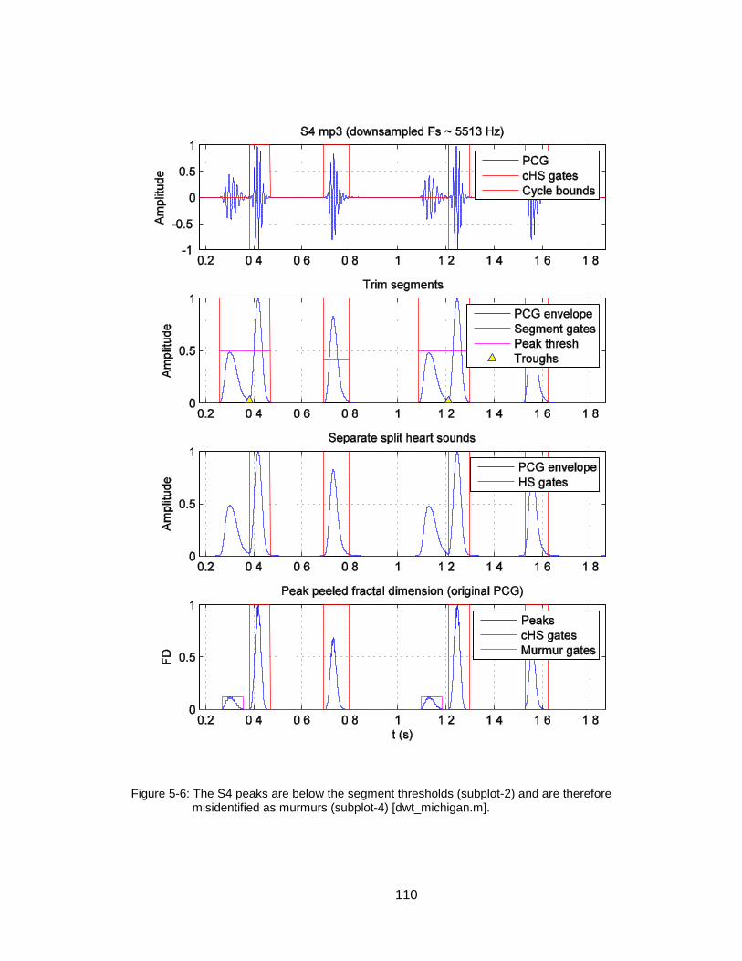
110
Figure 5-6: The S4 peaks are below the segment thresholds (subplot-2) and are therefore
misidentified as murmurs (subplot-4) [dwt_michigan.m].
111
Figure 5-7 illustrates the second and third type of error caused by trim_HS(). In the
first segment of the first heart cycle, which contains an S2 and an opening snap murmur,
the murmur is exempt from removal because its peak is above the threshold (subplot-2).
As a result, the murmur is misidentified as a split S2 component (subplot-3). In the second
segment of the first cycle, which contains an S1 and a late diastolic murmur, the murmur
is successfully removed because trim_HS() repositions the segment’s left boundary
(subplot-2). However, the segment’s right boundary is also repositioned even though a
systolic murmur does not exist within that segment. As a result, the portion of S1 that is
removed is misidentified as a murmur (subplot-4).

112
Figure 5-7: The opening snap murmur is misidentified as a split S2 component because the
murmur’s peak is above the threshold (subplot-2). Also, the right boundary of S1 is repositioned despite the lack of a systolic murmur, and the remaining piece is misidentified as a murmur [dwt_michigan.m].

113
Figure 5-8 illustrates an error that is unrelated to either energy thresholding or the
trim_HS() function. Here, find_heart_cycles() determines an incorrect distance between
cycle boundaries (subplot-1). This is because the PCG has a large amount of activity, so
the autocorrelation waveform is jagged, and a peak is detected near zero lag. This peak’s
magnitude is greater than the first spike located at a lag of one second, so it is misidentified
as the first heart cycle boundary. Segmentation therefore fails because the cycle durations
are too short.
Figure 5-8: The cycle durations are too short because a peak near zero lag is misidentified as a
heart cycle boundary [“AP.mp3”, dwt_littmann.m].

114
5.2.3 Wavelet Results
The wavelet-based segmentation errors described in the previous section are labeled
and summarized in Table 5-9. All of the murmur-containing sound files, as well as the
murmur-free sound files with detected errors, are listed in Table 5-10 (Michigan) and Table
5-11 (Littmann). For each sound file, the number of actual murmurs, detected true
murmurs, and heart cycles with detected false murmurs are listed; and the sound files are
labeled with their detected errors. This data is used to determine the TMDR in Table 5-12
and the FMDR in Table 5-13. Most of the sound files with detected errors either lower the
TMDR or increase the FMDR, or both, but certain sound files with detected errors do not
actually result in undetected true murmurs or detected false murmurs and therefore do not
affect those rates.
Table 5-9: Wavelet-based segmentation error labels and descriptions.
Error Process Description
E1-A
Energy thresholding
S1/S2 < HS threshold
E1-B S3/S4 < HS threshold
E1-C Murmur > HS threshold
E2-A
trim_HS()
HS peak < segment threshold
E2-B Murmur peak > segment threshold
E2-C Trough is identified as a junction between HS and murmur
E3 find_heart_cycles() Incorrect peak detected in the autocorrelation signal

115
Table 5-10: Wavelet-based segmentation results (Michigan).
Filename Error Total
Murmurs Detected true
murmurs
Heart cycles with detected false
murmurs
early dias murm E1-A 5 0 3
ejection click & syst eject murm & single S2
4 4 0
mid sys click 5 5 0
OS & dias murm E2-B E2-C
5 5 1
S3 & holosys murm E1-A 6 5 2
S4 & mid sys murm 5 5 0
sys click & late sys murm
5 5 0
sys murm & absent S2 6 6 0
sys & dias murm 6 6 0
sys eject murm & split S2 trans
E1-B 6 6 1
sys eject murm & split S2 pers
5 5 0
normal 2 E1-A 0 0 4
S3 E2-A 0 0 5
S4 E2-A 0 0 5
Total 58 52 21

116
Table 5-11: Wavelet-based segmentation results (Littmann).
Filename Errors Total
Murmurs Detected true
murmurs
Heart cycles with detected false murmurs
AP E3 4 0 0
AR 4 4 0
AS 3 3 0
ASD E1-C 4 2 0
COA 4 4 0
EA 6 6 0
eject click 2 2 0
eject click & AS moderate & AR mild
E2-B 4 4 0
innocent murmur 2 2 0
late sys click 4 4 0
mid sys click 3 3 0
MR severe E1-C 4 0 0
MS moderate E1-C 3 2 0
MVP 4 4 0
OS 2 2 0
PDA E1-A 4 2 0
S4 & AS severe 2 2 0
TR severe 4 4 0
VSD E1-C 4 2 0
S4 E1-B 0 0 0
sum gallop E1-B 0 0 2
Total 67 52 2
Table 5-12: Wavelet-based segmentation true murmur detection rate (TMDR).
Dataset Murmurs Detected true murmurs TMDR
Michigan 58 52 90%
Littmann 67 52 78%
Total 125 104 83%
Table 5-13: Wavelet-based segmentation false murmur detection rate (FMDR).
Dataset Heart
Cycles Heart cycles with
detected false murmurs FMDR
Michigan 101 21 21%
Littmann 76 2 3%
Total 177 23 13%

117
5.3 Simplicity-Based Segmentation
5.3.1 Simplicity Constants
The constants for simplicity-based segmentation, which consist of window lengths,
the peak peeling stopping condition, thresholds, and simplicity-specific values, are listed
in Table 5-14. All constants can be changed from their defaults using name-value pair
arguments passed to simpl_segment().
Table 5-14: Simplicity-based segmentation constants.
Constant Value Description
W 20 ms Fractal dimension and energy waveform window lengths
STC 10-4 Peak peeling stopping condition
N 10 ms Simplicity window length
m 2 ms Simplicity delay vector length
gamma 0.8 Coarseness of the PWC simplicity waveform
HS_thresh 0.6 Simplicity heart sound threshold
extra_HS_thresh 0.8 Simplicity extra heart sound threshold
WS 20 ms PCG smoothing window length
min_pk 0.2 min_height argument for split_HS() that specifies the minimum peak height for a split sound component
5.3.2 Simplicity Errors
Simplicity thresholding for simplicity-based segmentation is the functional equivalent
of energy thresholding for wavelet-based segmentation, except that the heart sound and
murmur segments are identified by their levels simplicity rather than their maximum
energies. As such, heart sound segments are misidentified as murmurs when their levels

118
are less than the heart sound threshold, and murmur segments are misidentified as heart
sounds when their levels are greater than the heart sound threshold.
Figure 5-9 illustrates how murmur segments can be misidentified as heart sounds
when their simplicity levels are greater than the normal heart sound threshold. This is the
same example used in Figure 5-5 for wavelet-based segmentation, so like before, the two
high-frequency systolic murmurs resemble typical murmurs, whereas the diastolic murmur
has low frequency content and resembles a heart sound (subplot-1). As a result, both of
the systolic murmurs are properly identified because their levels are less than the
threshold, but the diastolic murmur pieces are misidentified as heart sounds because their
levels are greater than the threshold (subplot-2).

119
Figure 5-9: The diastolic murmur is misidentified as a heart sound because its simplicity levels
are greater than the HS threshold (subplot-2) [simpl_littmann.m].

120
Figure 5-10 illustrates how at least one heart sound segment is required for
segmentation. Since all the segments’ levels are less than the normal heart sound
threshold, no heart sounds are detected (subplot-5). This is the same example used in
Figure 5-8 for wavelet-based segmentation, except that the error here occurs prior to
find_heart_cycles(), as heart cycle segmentation requires at least one heart sound
segment. Therefore, even though the segment levels are less than the threshold, the heart
sounds are not misidentified as murmurs because segmentation fails before sound
classification can occur.

121
Figure 5-10: No heart sounds are detected because all segment levels are less than the HS
threshold (subplot-5) [simpl_littmann.m].

122
The purpose of peak peeling for segmentation is to zero the low-amplitude noise
within the silent segments, so that the heart sounds and murmurs can be segmented.
Unfortunately, low amplitude murmurs may be inadvertently zeroed as well. In subplot-1
of Figure 5-11, a very low intensity diastolic murmur is not visible on the plot but can be
heard as a soft “wooshing” sound with headphones. Further proof of the murmur’s
existence can be seen in the simplicity waveform in subplot-3. The high simplicity values
in systole are typical of the attenuated and smoothed noise in the silent segments, but the
moderate simplicity values in diastole, which are lower than those in S1 and S2, are
characteristic of murmurs. Since the murmurs here are so soft, their time-domain values
are not transformed into fractal values of sufficient amplitude, so they are zeroed during
peak peeling (subplot-2). The zero-valued samples in the peak peeled fractal dimension
are then used to zero the corresponding samples in the simplicity waveform (subplot-4).
As a result, the murmurs cannot be segmented because their simplicity levels are set to
zero. This is a rare error because most heart sounds are loud enough to be transformed
into a suitable fractal value (and to also be visible on the plot) and are therefore not
removed during peak peeling. Nonetheless, this example demonstrates how the
amplitude-invariant simplicity transform can be limited by the fractal dimension.

123
Figure 5-11: The low amplitude diastolic murmurs (not visible) are undetected because they were
zeroed while peak peeling the fractal dimension (subplot-2). The corresponding simplicity values are zeroed (subplot-4), so the murmurs are not segmented (subplot-5) [simpl_michigan.m].

124
Even though distinguishing extra heart sounds from split sound components is not a
requirement for successful segmentation, misidentifying extra heart sounds can affect the
segmentation of normal heart sounds in certain scenarios. This is illustrated in Figure 5-12,
where the simplicity levels of the summation gallops are greater than the S1 and S2 levels
but are nonetheless less than the extra heart sound threshold. As a result, the summation
gallops are misidentified as normal heart sounds (subplot-2), and since S2 and the
summation gallop are separated by less than sscope.min_syst_dur samples, they are
further misidentified as split sound components. Unfortunately, the distance separating
the “split” sounds from S1 is less than the distance separating S1 from S2, so systole and
diastole, and therefore S1 and S2, are switched.

125
Figure 5-12: The summation gallops are misidentified as split sound components because their
simplicity levels are less than the extra HS threshold (subplot-2). This causes systole and diastole, and therefore S1 and S2, to be switched (subplot-1) [simpl_littmann.m].

126
5.3.3 Simplicity Error Tables
The simplicity-based segmentation errors described in the previous section are
labeled and summarized in Table 5-15. All the murmur-containing sound files, as well as
the murmur-free sound files with detected errors, are listed in Table 5-16 (Michigan) and
Table 5-17 (Littmann). For each sound file, the number of actual murmurs, detected true
murmurs, and cycles with detected false murmurs are listed; and the sound files are
labeled with their detected errors. This data is used to determine the TMDR in Table 5-18
and the FMDR in Table 5-19. Most sound files with detected errors either lower the TMDR
or increase the FMDR, or both, but certain sound files with detected errors do not actually
cause undetected true murmurs or detected false murmurs and therefore do not affect
those rates at all.
Table 5-15: Simplicity-based segmentation error labels and descriptions.
Error Process Description
E1-A
Simplicity thresholding
S1/S2 < normal HS threshold
E1-B Murmur > normal HS threshold
E1-C S3/S4 < extra HS threshold
E2 Peak peeling Soft murmurs are removed

127
Table 5-16: Simplicity-based segmentation results (Michigan).
Filename Errors Murmurs Detected true
murmurs
Cycles with detected false
murmurs
early dias murm E2 5 0 0
ejection click & syst eject murm & single S2
4 4 0
mid sys click 5 5 0
OS & dias murm E1-B 5 4 0
S3 & holosys murm 6 6 0
S4 & mid sys murm 5 5 0
sys click & late sys murm
5 5 0
sys murm & absent S2
6 6 0
sys & dias murm 6 6 0
sys eject murm & split S2 trans
6 6 0
sys eject murm & split S2 pers
5 5 0
Total 58 52 0

128
Table 5-17: Simplicity-based segmentation results (Littmann).
Filename Errors Murmurs Detected
true murmurs
Cycles with detected false
murmurs
AP E1-A 4 0 0
AR 4 4 0
AS 3 3 0
ASD E1-B 4 2 0
COA 4 4 0
EA 6 6 0
eject click 2 2 0
eject click & AS moderate & AR mild
4 4 0
innocent murmur 2 2 0
late sys click 4 4 0
mid sys click 3 3 0
MR severe E1-B 4 2 0
MS moderate E1-B 3 0 0
MVP 4 4 0
OS 2 2 0
PDA E1-A 4 2 0
S4 & AS severe 2 2 0
TR severe 4 4 0
VSD E1-B 4 2 0
sum gallop E1-C 0 0 0
Total 67 52 0
Table 5-18: Simplicity true murmur detection rate (TMDR).
Dataset Murmurs Detected true
murmurs TMDR
Michigan 58 52 90%
Littmann 67 52 78%
Total 125 104 83%
Table 5-19: Simplicity false murmur detection rate (FMDR).
Dataset Cycles Cycles with detected
false murmurs FMDR
Michigan 101 0 0%
Littmann 76 0 0%
Total 177 0 0%
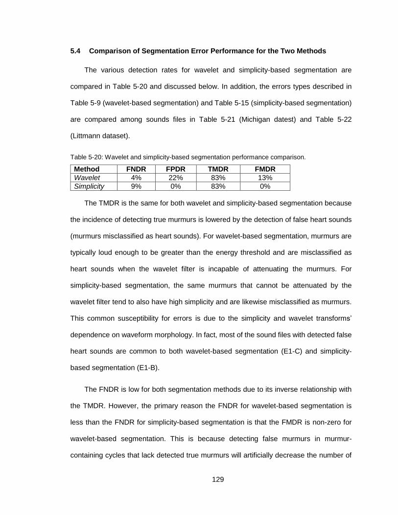
129
5.4 Comparison of Segmentation Error Performance for the Two Methods
The various detection rates for wavelet and simplicity-based segmentation are
compared in Table 5-20 and discussed below. In addition, the errors types described in
Table 5-9 (wavelet-based segmentation) and Table 5-15 (simplicity-based segmentation)
are compared among sounds files in Table 5-21 (Michigan datest) and Table 5-22
(Littmann dataset).
Table 5-20: Wavelet and simplicity-based segmentation performance comparison.
Method FNDR FPDR TMDR FMDR
Wavelet 4% 22% 83% 13%
Simplicity 9% 0% 83% 0%
The TMDR is the same for both wavelet and simplicity-based segmentation because
the incidence of detecting true murmurs is lowered by the detection of false heart sounds
(murmurs misclassified as heart sounds). For wavelet-based segmentation, murmurs are
typically loud enough to be greater than the energy threshold and are misclassified as
heart sounds when the wavelet filter is incapable of attenuating the murmurs. For
simplicity-based segmentation, the same murmurs that cannot be attenuated by the
wavelet filter tend to also have high simplicity and are likewise misclassified as murmurs.
This common susceptibility for errors is due to the simplicity and wavelet transforms’
dependence on waveform morphology. In fact, most of the sound files with detected false
heart sounds are common to both wavelet-based segmentation (E1-C) and simplicity-
based segmentation (E1-B).
The FNDR is low for both segmentation methods due to its inverse relationship with
the TMDR. However, the primary reason the FNDR for wavelet-based segmentation is
less than the FNDR for simplicity-based segmentation is that the FMDR is non-zero for
wavelet-based segmentation. This is because detecting false murmurs in murmur-
containing cycles that lack detected true murmurs will artificially decrease the number of

130
false negative cycles. This is aptly demonstrated in the sound file early dias murm from
the Michigan dataset. For simplicity-based segmentation, all five cycles are false
negatives because the soft murmurs were zeroed through peak peeling (E2). For wavelet-
based segmentation, the same murmurs were also zeroed through peak peeling; however,
only two of the cycles are false negatives because false murmurs were detected in the
other three cycles. Therefore, the FNDR is suitable for clinical evaluations, but a full
performance evaluation of the two methods can only be achieved by comparing the TMDR
and FMDR. As a result, simplicity-based segmentation, despite having the same TMDR
as wavelet-based segmentation, is superior in this regard because its FMDR is zero.
The FMDR is non-zero for wavelet-based segmentation because heart sounds are
often soft enough to be less than the heart sound energy threshold and therefore
misclassified as murmurs (E1-A and E1-B). Furthermore, trim_HS() is prone to splitting
heart sound segments and creating unnecessary murmurs (E2-A and E2-C). In contrast,
the FMDR is zero for simplicity-based segmentation because the simplicity waveform is
amplitude invariant. Since heart sounds have relatively high simplicity, it is rare for them
to be misclassified as murmurs or noise (low simplicity). In addition, the gamma constant
for the L2 Potts minimization function is the equivalent of trim_HS() for simplicity-based
segmentation because both are used to determine the optimal boundaries between
merged heart sounds and murmurs. Nonetheless, the two are hardly equivalent in
outcome because locating the segment boundaries using the piecewise constant
approximation function on the simplicity waveform is a far more accurate and less error
prone method than is using energy thresholding and trim_HS().
The FPDR, as a subset of the FMDR, is likewise non-zero for wavelet-based
segmentation but zero for simplicity-based segmentation. The only reason the FPDR is

131
greater than the FMDR, at least for these datasets, is that a higher proportion of false
murmurs are detected in the murmur-free cycles than are detected in all cycles.
Table 5-21: Wavelet and simplicity-based segmentation error comparisons (Michigan).
Filename Wavelet Simplicity
early dias murm E1-A E2
ejection click & syst eject murm & single S2
mid sys click
OS & dias murm E2-B E2-C
E1-B
S3 & holosys murm E1-A
S4 & mid sys murm
sys click & late sys murm E2
sys murm & absent S2
sys & dias murm
sys eject murm & split S2 trans
E1-B
sys eject murm & split S2 pers
normal 1
normal 2 E1-A
S3 E2-A
S4 E2-A
single S2
split S1 pers
split S2 pers
split S2 trans

132
Table 5-22: Wavelet and simplicity-based segmentation error comparisons (Littmann)
File Name Wavelet Simplicity
AP E3 E1-A
AR
AS
ASD E1-C E1-B
COA
EA
eject click
eject click & AS moderate & AR mild
E2-B
innocent murmur
late sys click
mid sys click
MR severe E1-C E1-B
MS moderate E1-C E1-B
MVP
OS
PDA E1-A E1-A
S4 & AS severe
TR severe
VSD E1-C E1-B
normal
S3 & S4
S3 abnormal
S3 physio
S4 E1-B
sum gallop E1-B E1-C
split S2 fixed
split S2 physio
split S1
133
6 Conclusions and Future Work
The results from Chapter 5 demonstrate how simplicity-based segmentation is
superior to wavelet-based segmentation. This is because the simplicity transform is
amplitude invariant and, in combination with Pottslab’s piecewise constant denoising
algorithm, is able to determine each sound segment’s optimal boundaries, assign a single
simplicity value to each segment, and then classify the sound segments according to their
simplicity levels. This is in contrast to wavelet-based segmentation, which must attenuate
the murmurs to segment the heart sounds, remove non-attenuated or partially attenuated
murmur segments by energy thresholding, and use the PCG waveform to remove any
murmurs merged with heart sounds. As a result, the incidence of false murmurs, and
therefore false positives, is significant. Despite the comparable false negative and true
murmur detection rates for both methods, simplicity-based segmentation is ultimately
preferable due to its zero false positive and false murmur detection rates.
Even though both segmentation methods are adequate for detecting and classifying
murmurs, certain aspects of the system could be improved. One improvement could be
applied to the heart cycle segmentation function, find_heart_cycles(). This function
determines the heart cycle boundaries by locating the largest peak in the autocorrelation
waveform, which should resemble a spike and be located on the first heart cycle’s stop
boundary, and then places the remaining heart cycle boundaries at integer multiples of
the first peak’s location. Unfortunately, this function is currently incapable of verifying
whether or not the largest peak is a prominent spike rather than a small fluctuation. This
could be improved by setting a minimum acceptable peak prominence, or height relative
to surrounding troughs, by using the ‘MinPeakProminence’ option for findpeaks(), which
is only available in MATLAB 2015.

134
Another suggested improvement would replace the simple thresholds used during
simplicity-based segmentation with a clustering algorithm. Rather than manually choosing
an optimal threshold, sound segment features such as pitch, location, shape, and duration
could be placed in a feature vector, and the algorithm would use these features to classify
each sound segment as either a normal heart sound, extra heart sound, or murmur.
Finally, even though the purpose of this system is to detect and classify murmurs as either
systolic or diastolic, it is also desirable to further categorize the murmurs by their specific
types, such as aortic stenosis, mitral regurgitation, atrial septal defect, etc. This could be
achieved by reusing the feature vector from the clustering operation as an input to an
artificial neural network. This would require training the network with a select dataset of
PCG’s, so that murmur segments from clinical PCG’s could be completely and accurately
classified.

135
REFERENCES
[1] J. Doohan, "The Circulatory System," Santa Barbara City College, 17 September
1999. [Online]. Available: http://www.biosbcc.net/doohan/sample/htm/heart.htm.
[Accessed 18 February 2016].
[2] Wapcaplet, Diagram of the Human Heart (Cropped), Wikimedia Commons.
[3] R. Klabunde, "Cardiac Cycle," 2 January 2011. [Online]. Available:
http://www.cvphysiology.com/Heart%20Disease/HD002.htm. [Accessed 19
February 2016].
[4] M. R. Villarreal, Human Heart during Systole and Diastole, Wikimedia Commons,
2008.
[5] P. Kubin, "The Stethoscope and How to Use It," 4 November 2012. [Online].
Available: http://www.mypatraining.com/stethoscope-and-how-to-use-it. [Accessed
20 April 2015].
[6] S. Lome, "Heart Murmurs," Healio, [Online]. Available:
http://www.healio.com/cardiology/learn-the-heart/cardiology-review/heart-murmurs.
[Accessed 20 April 2015].
[7] "Phonocardiography," Encyclopaedia Britannica., 2016. [Online]. Available:
http://www.britannica.com/science/phonocardiography. [Accessed 27 February
2016].
[8] S. Lome, "Heart Sounds," [Online]. Available:
http://www.learntheheart.com/cardiology-review/heart-sounds/. [Accessed 20 April
2015].

136
[9] A. Kumar and T. V. Ananthapadmanabha, "Heart Rate Variability using Shannon
Energy," SASTech, vol. V, no. 2, pp. 23-26, 2006.
[10] L. J. Hadjileontiadis and I. T. Rekanos, "Detection of Explosive Lung and Bowel
Sounds by Means of Fractal Dimension," IEEE Signal Processing Letters, vol. 10,
no. 10, pp. 311-314, 2003.
[11] L. J. Hadjileontiadis, "Wavelet-Based Enhancement of Lung and Bowel Sounds
Using Fractal Dimension Thresholding—Part I: Methodology," IEEE Transactions
on Biomedical Engineering, vol. 52, no. 6, pp. 1143-1148, 2005.
[12] N. A. a. T. Ning, "Isolation of Systolic Heart Murmurs Using Wavelet Transform and
Energy Index," in Congress on Image and Signal Processing, 2008.
[13] V. Nigam and R. Priemer, "Accessing heart dynamics to estimate durations of heart
sounds," Institute of Physics Publishing, vol. 26, pp. 1005-1018, 2005.
[14] D. Kumar, P. Carvalho, M. Antunes, J. Henriques, M. Maldonado, R. Schmidt and
J. Habetha, "Wavelet Transform and Simplicity Based Heart Murmur
Segmentation," Computers in Cardiology, vol. 33, pp. 173-176, 2006.
[15] M. A. Little and N. S. Jones, "Generalized Methods and Solvers for Noise Removal
from Piecewise Constant Signals. I. Background Theory.," Proceedings of the
Royal Society, vol. 471, no. 2177, 8 June 2011.
[16] A. Weinmann, M. Storath and L. Demaret, "The L1-Potts Functional for Robust
Jump-Sparse Reconstruction," arXiv:1207.4642, 2012.
[17] M. Storath, A. Weinmann and L. Demaret, "Jump-Sparse and Sparse Recovery
Using Potts Functionals," IEEE Transactions on Signal Processing, vol. 62, no. 14,
pp. 3654-3666, 2014.

137
[18] M. Storath and A. Weinmann, "Fast Partitioning of Vector-Valued Images," SIAM
Journal on Imaging Sciences, vol. 7, no. 3, pp. 1826-1852, 2014.
[19] Assessment Technologies Institute, "Cardiac Examination," Assessment
Technologies Institute, [Online]. Available:
http://atitesting.com/ati_next_gen/skillsmodules/content/physical-assessment-
adult/equipment/cardiac.html. [Accessed 28 February 2016].
[20] S. G. Wong, "Design, Characterization, and Application of a Multiple Input
Stethoscope Apparatus," California Polytechnic State University, San Luis Obispo,
2014.
[21] I. McCowan, Microphone Arrays: A Tutorial, 2001.
[22] J. Scampini, "Overview of Ultrasound Imaging Systems and the Electrical
Components Required for Main Subfunctions," Maxim Integrated, 10 May 2010.
[Online]. Available: https://www.maximintegrated.com/en/app-
notes/index.mvp/id/4696. [Accessed 14 Feb 2016].
[23] Andeggs, Artist, 3D spherical coordinates. [Art]. Wikimedia Commons, 2009.
[24] D. Blanford and J. Parr, Introduction to Digital Signal Processing, Upper Saddle
River: Pearson, 2013.
[25] A. Ambardar, Analog and Digital Signal Processing, Pacific Grove: Brooks/Cole,
1999.
[26] B. Stern, "The Basic Concepts of Diagnostic Ultrasound1," Yale-New Haven
Teachers Institute, [Online]. Available:
http://www.yale.edu/ynhti/curriculum/units/1983/7/83.07.05.x.html. [Accessed 15 7
2016].
138
[27] J. Meiss, "Dynamical Systems," Scholarpedia, 2007. [Online]. Available:
http://www.scholarpedia.org/article/Dynamical_system. [Accessed 8 May 2016].
[28] "The Ptolemaic Model," Iowa State University, 2001. [Online]. Available:
http://www.polaris.iastate.edu/EveningStar/Unit2/unit2_sub1.htm. [Accessed 6 May
2016].
[29] T. D. Sauer, "Attractor Reconstruction," Scholarpedia, 2006. [Online]. Available:
http://www.scholarpedia.org/article/Attractor_reconstruction. [Accessed 8 May
2016].
[30] A. Leon-Garcia, Probability, Statistics, and Random Processes for Electrical
Engineering, Upper Saddle River: Pearson Prentice Hall, 2008.
[31] J. Rossel, Artist, Functional approximatin of square wave using 5 harmonics. [Art].
Wikimedia Commons, 2010.
[32] A. W. Martin Storath, "Pottslab," [Online]. Available: http://pottslab.de/. [Accessed
15 July 2016].
[33] "Heart and Lung Sounds," 3M, [Online]. Available:
http://www.3m.com/healthcare/littmann/mmm-library.html. [Accessed 16 7 2016].
[34] M. Rajesh S. Mangrulkar and M. Richard D. Judge, "Heart Sound and Murmur
Library," University of Michigan Medical School, Ann Arbor. [Online].

139
APPENDICES

140
A. Scripts
A.1 Examples
A.1.1 chp4_seg.m
clear; clc; close all lvl1 = 2; lvl2 = 5; %% Split S2 (persistent) close all stethoscope('michigan', 'split S2 pers.mp3', lvl1, 'show_filt', true); %% Systolic ejection murmur & split S2 (persistent) close all sscope = stethoscope('michigan', 'sys eject murm & split S2 pers.mp3', lvl1); sscope = dwt_segment(sscope, lvl2, 'show', 'seg'); plot(sscope) %% Systolic murmur & absent S2 close all sscope = stethoscope('michigan', 'sys murm & absent S2.mp3', lvl1); dwt_segment(sscope, lvl2, 'show', { 'seg'%, ... % 'peak_peel', ... % 'find_cyc' }); %% Split S2 (fixed) close all sscope = stethoscope('littmann', 'split S2 fixed.mp3', lvl1); dwt_segment(sscope, lvl2, 'show', 'seg'); %% S3 & holosystolic murmur close all sscope = stethoscope('michigan', 'S3 & holosys murm.mp3', lvl1); simpl_segment(sscope, 'show', 'seg');
A.1.2 energy_functions.m
% Shannon energy vs squared energy curves clear; close all; clc x = linspace(0, 1, 101); shannon = x.^2 .* log(x.^2); squared = x.^2; figure('color','w') hold on plot(x, squared) plot(x, -shannon, 'm') grid on

141
box on ylabel('E(x)') xlabel('x') legend('Squared energy - x^2', 'Shannon energy - x^2log(x^2)', ... 'Location', 'northwest') title('Energy functions')
A.1.3 heart_sounds.m
clear; clc; close all folder = fullfile('PCG', 'michigan'); max_dur = 3; ds = 'dyadic'; Fs_min = 4e3; yl = [-1, 1]; xlbl = 't (s)'; ylbl = 'Amplitude'; %% Split S2 close all path = fullfile(folder, 'split S2 pers.mp3'); [split_S2, Fs] = load_PCG(path, max_dur, ds, Fs_min); t = time(split_S2, Fs); figure plot(t, split_S2) ylim(yl) xlabel(xlbl) ylabel(ylbl) title('Split S2 Example') plot_style(gca) %% S3 close all path = fullfile(folder, 'S3.mp3'); [S3, Fs] = load_PCG(path, max_dur, ds, Fs_min); t = time(S3, Fs); figure plot(t, S3) ylim(yl) xlabel(xlbl) ylabel(ylbl) title('S3 Example') plot_style(gca) %% S4 close all path = fullfile(folder, 'S4.mp3'); [S4, Fs] = load_PCG(path, max_dur, ds, Fs_min); t = time(S4, Fs); figure plot(t, S4)

142
ylim(yl) xlabel(xlbl) ylabel(ylbl) title('S4 Example') plot_style(gca) %% Normal close all path = fullfile(folder, 'normal 2.mp3'); [normal, Fs] = load_PCG(path, max_dur, ds, Fs_min); t = time(normal, Fs); figure plot(t, normal) ylim(yl) xlabel(xlbl) ylabel(ylbl) title('Normal Heart Sound Example') plot_style(gca)
A.1.4 PCG_FFT.m
% Compare the spectra of S1, S2, and murmur. clc; close all; clear % Load the PCG file = 'sys eject murm & split S2 pers.mp3'; path = fullfile('PCG', 'michigan', file); lim = [1.9, 2.6]; [PCG, Fs, offset] = load_PCG(path, lim, 4e3, 'dyadic'); % Set segment boundaries bnds = [1.98, 2.06, 2.3, 2.38, 2.49]*Fs - offset + 1; S1 = segment(bnds(1), bnds(2)); murm = segment(S1.stop+1, bnds(3)); A2 = segment(murm.stop+1, bnds(4)); P2 = segment(A2.stop+1, bnds(5)); % FFT [S1_resp, S1_freq] = nfft(PCG(S1.rng)); [murm_resp, murm_freq] = nfft(PCG(murm.rng)); [A2_resp, A2_freq] = nfft(PCG(A2.rng)); [P2_resp, P2_freq] = nfft(PCG(P2.rng)); % Plot figure [t, xl] = time(PCG, Fs, lim(1)); ax(1) = subplot(211); plot(t, PCG) xlim(xl) xlabel('t (s)') ylabel('Amplitude') title(pcg_descr(file, Fs)) ax(2) = subplot(212);

143
hold on plot(S1_freq*Fs, abs(S1_resp), 'b') plot(A2_freq*Fs, abs(A2_resp), 'r') plot(P2_freq*Fs, abs(P2_resp), 'm') plot(murm_freq*Fs, abs(murm_resp), 'g') xlim([0, 500]) legend('S1', 'A2', 'P2', 'Murmur') xlabel('f (Hz)') ylabel('Magnitude') title('FFT - Magnitude Response') plot_style(ax)
A.1.5 PCG_simpl.m
% Demonstrate the simplicity transform of a PCG. clear; clc; close all % Load the PCG file = 'normal 1.mp3'; path = fullfile('PCG', 'michigan', file); lim = [0.3, 1.8]; [PCG, Fs] = load_PCG(path, lim, 4e3, 'dyadic'); % Simplicity N = 10e-3*Fs; m = 2e-3*Fs; simpl = st(PCG, m, N); % Plot figure [t, xl] = time(PCG, Fs, lim(1)); ax(1) = subplot(211); plot(t, PCG) xlabel('t (s)') ylabel('Amplitude') title(pcg_descr(file, Fs)) ax(2) = subplot(212); plot(t, simpl) xlabel('t (s)') ylabel('Simplicity') title('Simplicity transform') plot_style(ax, xl)
A.1.6 rect_sinc.m
% Compare rect(t) and its Fourier transform sinc(f). clc; close all; clear npts = 1000; % time axis t1 = -1;

144
t2 = 1; t = linspace(t1, t2, npts); % freq axis f1 = -4; f2 = 4; f = linspace(f1, f2, npts); nodes = [(f1:-1), (1:f2)]; % zero crossings % Plot figure yl = [-0.5, 1.5]; ax(1) = subplot(211); plot(t, rect(t, 0.5)) ylim(yl) set(gca, 'XTick', t1:0.5:t2) xlabel('t') ylabel('x(t)') title('rect(t)') ax(2) = subplot(212); hold on plot(f, sinc(f)) plot(nodes, sinc(nodes), 'o', 'color', 'red'); ylim(yl) set(gca, 'XTick', f1:f2) xlabel('f') ylabel('|X(f)|') title('sinc(f)') plot_style(ax)
A.1.7 singular_spectra.m
% Compare the singular spectra of sinc and white gaussian noise. clc; close all; clear npts = 1000; t = linspace(-10, 10, npts).'; % noise = "complex" pwr = 0; load = 50; noise = wgn(npts, 1, pwr, load, 'dBm'); % sinc = "simple" sinc = sinc(t); % singular spectra m = 10; [~, D_noise] = st(noise, m); [~, D_sinc] = st(sinc, m); % Plot figure % Signals ax(1) = subplot(221);

145
plot(t, noise) xlabel('t (s)') ylabel('Amplitude') title(sprintf('White Gaussian Noise (%d dBm, %d \\Omega)', pwr, load)) ax(3) = subplot(223); plot(t, sinc) ylim([-0.4, 1.2]) xlabel('t (s)') ylabel('Amplitude') title('sinc(t)') % Singular spectra xl = [0, numel(D_sinc)+1]; yl = [0, 1]; ax(2) = subplot(222); stem(D_noise) xlim(xl) ylim(yl) xlabel('Index') ylabel('Eigenvalue') title('Singular spectrum (noise)') ax(4) = subplot(224); stem(D_sinc) xlim(xl) ylim(yl) xlabel('Index') ylabel('Eigenvalue') title('Singular spectrum (sinc)') set([ax(2), ax(4)], 'YTick', 0:0.2:1); plot_style(ax)
A.2 Results
A.2.1 batch.m
% Batch segment all sound files clear; close all; clc root = 'C:\Users\Josh\Google Drive\thesis\matlab'; lvl1 = 2; lvl2 = 5; %% DWT % Michigan dwt = @(s) dwt_segment(s, lvl2); batch_segment(dwt, root, 'michigan', lvl1) % Littmann dwt = @(s) dwt_segment(s, lvl2, 'HS_thresh', 0.05); batch_segment(dwt, root, 'littmann', lvl1) %% Simplicity
146
% Michigan simpl = @(s) simpl_segment(s); batch_segment(simpl, root, 'michigan', lvl1) % Littmann simpl = @(s) simpl_segment(s); batch_segment(simpl, root, 'littmann', lvl1)
A.2.2 beamforming.m
% Plot the directivity pattern of a non-uniformly spaced planar stethoscope % array after beamforming. clear; clc; close all dir = 'C:\Users\Josh\Google Drive\thesis\matlab\figures\chp2\'; fmt = 'epsc'; store = false; %% Specify stethoscope locations % Relative to the origin (inches) x = [-2.11, -2.03, 1.91, 2.25, 0]; y = [-0.938, 1.29, 0.887, -1.23, 0]; z = zeros(size(y)); % Convert to meters r = [x; y; z]*0.0254; %% Plot stethoscope locations fig = figure('color', 'white'); plot(x, y, 'o', 'MarkerSize', 10, 'MarkerFaceColor', 'b') xlabel('x') ylabel('y') title('Relative stethoscope positions (meters)') grid on box on % Save if ~isempty(dir) set(fig, 'PaperUnits', 'inches', 'PaperPosition', [0, 0, 6, 4]) saveas(gcf, fullfile(dir, 'stethoscope_locations'), fmt) end %% Beamform % Average speed of sound in tissue (m/s) v = 1540; % Frequencies of interest freq(1) = 500; % innside heart murmur range freq(2) = 7e3; % outside of heart murmur range (no spatial aliasing) freq(3) = 20e3; % outside of heart murmur range (spatial aliasing) % Target angles theta_t = pi/2; phi_t = (0:1/6:1) * pi; % Resolution npts = 500; % Sweep for f = freq fprintf('Frequency = %.0e Hz\n', f) isAliased(r, f, v, 'm', 3); % check for spatial aliasing

147
fprintf('\n') for i = 1:numel(phi_t) beam_pattern(r, f, v, theta_t, phi_t(i), npts) % Save if store fig = gcf; set(fig, 'PaperUnits', 'inches', 'PaperPosition', [0, 0, 6, 2]) fn = sprintf('%.0eHz_%d', f, i); saveas(fig, fullfile(dir, fn), fmt) close end end end
A.2.3 dwt_michigan.m
clear; close all; clc file = [ % MURMURS % 'early dias murm.mp3' % E1A % 'eject click & sys eject murm & single S2.mp3' % 'mid sys click.mp3' % 'OS & dias murm.mp3' % E2B, E2C % 'S3 & holosys murm.mp3' % E1A % 'S4 & mid sys murm.mp3' % 'sys click & late sys mur.mp3' % 'sys murm & absent S2.mp3' % 'sys & dias murm.mp3' % 'sys eject murm & split S2 trans.mp3' % E1B % 'sys eject murm & split S2 pers.mp3' % NO MURMURS % 'normal 1.mp3' % 'normal 2.mp3' % E1A % 'S3.mp3' % E2A % 'S4.mp3' % E2A % 'single S2.mp3' % 'split S1 pers.mp3' % 'split S2 pers.mp3' % 'split S2 trans.mp3' ]; sscope = stethoscope('michigan', file, 2); sscope = dwt_segment(sscope, 5, 'show', 'seg'); print(sscope) % plot(sscope)
A.2.4 dwt_littmann.m
clear; close all; clc file = [ % MURMURS
148
% 'AP.mp3' % E4 % 'AR.mp3' % 'AS.mp3' % 'ASD.mp3' % E1C % 'COA.mp3' % 'EA.mp3' % 'eject click.mp3' % 'eject click & AS moderate & AR mild.mp3' % E2B % 'innocent murmur.mp3' % 'late sys click.mp3' % 'mid sys click.mp3' % 'MR severe.mp3' % E1C % 'MS moderate.mp3' % E1C % 'MVP.mp3' % 'OS.mp3' % 'PDA.mp3' % E1A % 'S4 & AS severe.mp3' % 'TR severe.mp3' % 'VSD.mp3' % E1C % NO MURMURS % 'normal.mp3' % 'S3 & S4.mp3' % 'S3 abnormal.mp3' % 'S3 physio.mp3' % 'S4.mp3' % E1B % 'sum gallop.mp3' % E1B % 'split S2 fixed.mp3' % 'split S2 physio.mp3' % 'split S1.mp3' ]; sscope = stethoscope('littmann', file, 2); sscope = dwt_segment(sscope, 5, 'HS_thresh', 0.05, 'show', 'seg'); print(sscope) % plot(sscope)
A.2.5 simpl_michigan.m
clear; close all; clc file = [ % MURMURS % 'early dias murm.mp3' % E2 % 'eject click & sys eject murm & single S2.mp3' % 'mid sys click.mp3' % 'OS & dias murm.mp3' % E1B % 'S3 & holosys murm.mp3' % 'S4 & mid sys murm.mp3' % 'sys click & late sys mur.mp3' % 'sys murm & absent S2.mp3' % 'sys & dias murm.mp3' % 'sys eject murm & split S2 trans.mp3' % 'sys eject murm & split S2 pers.mp3'

149
% NO MURMURS % 'normal 1.mp3' % 'normal 2.mp3' % 'S3.mp3' % 'S4.mp3' % 'single S2.mp3' % 'split S1 pers.mp3' % 'split S2 pers.mp3' % 'split S2 trans.mp3' ]; sscope = stethoscope('michigan', file, 2); sscope = simpl_segment(sscope, 'show', 'seg'); print(sscope) % plot(sscope)
A.2.6 simpl_littmann.m
clear; close all; clc file = [ % MURMURS % 'AP.mp3' % E1A % 'AR.mp3' % 'AS.mp3' % 'ASD.mp3' % E1B % 'COA.mp3' % 'EA.mp3' % 'eject click.mp3' % 'eject click & AS moderate & AR mild.mp3' % 'innocent murmur.mp3' % 'late sys click.mp3' % 'mid sys click.mp3' % 'MR severe.mp3' % E1B % 'MS moderate.mp3' % E1B % 'MVP.mp3' % 'OS.mp3' % 'PDA.mp3' % E1A % 'S4 & AS severe.mp3' % 'TR severe.mp3' % 'VSD.mp3' % E1B % NO MURMURS % 'normal.mp3' % 'S3 & S4.mp3' % 'S3 abnormal.mp3' % 'S3 physio.mp3' % 'S4.mp3' % 'sum gallop.mp3' % A % 'split S2 fixed.mp3' % 'split S2 physio.mp3' % 'split S1.mp3' ]; sscope = stethoscope('littmann', file, 2);

150
sscope = simpl_segment(sscope, 'show', 'seg'); print(sscope) % plot(sscope)

151
B. Functions
B.1 Beamforming
B.1.1 beam_pattern.m
% BEAM_PATTERN(r, f, v, theta_t, phi_t, npts) % % Plot the beam pattern after steering it towards the target angles. % % Args: % r: position matrix [x_vec; y_vec; z_vec] % f: frequency of interest % v: wave velocity % theta_t: target theta % phi_t: target phi % npts: # of points for theta and phi vectors function beam_pattern(r, f, v, theta_t, phi_t, npts) [D, theta, phi] = beamform(r, f, v, theta_t, phi_t, npts); % Separate theta and phi axes theta_vec = theta(1,:); % any row phi_vec = phi(:,1); % any col % D vs (target theta, phi) i = closest(theta_vec, theta_t); D_phi = abs(D(:,i)); % fix theta % phi @ maximum intensity [~, i] = max(D_phi); max_phi = phi_vec(i); % D vs (theta, target phi) i = closest(phi_vec, phi_t); D_theta = abs(D(i,:)); % fix phi % theta @ maximum intensity [~, i] = max(D_theta); max_theta = theta_vec(i); % Convert angles to strings phi_str = pi2ratstr(phi_t); theta_str = pi2ratstr(theta_t); % Plot figure('color', 'white') % 2D polar plot vs phi @ target theta subplot(121) polar(phi_vec, D_phi); xlabel('\phi') str = sprintf('\\phi_{target} = %s, \\theta = %s', phi_str, theta_str); title(str) % Arrow pointing to target phi hold on compass(cos(max_phi), sin(max_phi), 'r');

152
% 2D polar plot vs theta @ target phi subplot(122) polar(theta_vec, D_theta) xlabel('\theta') str = sprintf('\\theta_{target} = %s, \\phi = %s', theta_str, phi_str); title(str) % Arrow pointing to target theta hold on compass(cos(max_theta), sin(max_theta), 'r'); end function str = pi2ratstr(x) % Factor out pi from numerator [N, D] = rat(x / pi); % Convert to LaTex interpreted string if N > 1 num = sprintf('%d%s', N, '\pi'); elseif N == 1 num = '\pi'; else str = '0'; return end if D > 1 str = sprintf('%s/%d', num, D); else str = sprintf('%s', num); end end
B.1.2 beamform.m
% [D, theta, phi] = BEAMFORM(r, f, v, theta_t, phi_t, npts) % % Steer the beam pattern towards the target angles by applying an angular % dependent phase weight to each sensor. % % Args: % r: position matrix [x_vec; y_vec; z_vec] % f: frequency of interest % v: wave velocity % theta_t: target theta % phi_t: target phi % npts: # of points for theta and phi vectors % % Returns: % D: directivity pattern (matrix) % theta: polar angles (matrix) % phi: azimuthal angles (matrix) function [D, theta, phi] = beamform(r, f, v, theta_t, phi_t, npts) f = abs(f); v = abs(v); % theta = row, phi = column gv = linspace(0, 2*pi, npts); [theta, phi] = meshgrid(gv);

153
% d(x,y,z) = beta(x,y,z) - beta'(x,y,z) dx = sin(theta) .* cos(phi) - sin(theta_t) .* cos(phi_t); dy = sin(theta) .* sin(phi) - sin(theta_t) .* sin(phi_t); dz = cos(theta) - cos(theta_t); % Calculate the array's directivity pattern D = zeros(size(theta)); omega = 2*pi * f; N = size(r,2); % # of sensors for n = 1:N dot_prod = (r(1,n) .* dx) + (r(2,n) .* dy) + (r(3,n) .* dz); D = D + exp(-1j .* omega ./ v .* dot_prod); end D = D / N; % normalize end
B.1.3 dist_mat.m
% dist = DIST_MAT(r) % % Calculate the distance between all possible pairs of points in the position % matrix r = [x_vec; y_vec; z_vec], and store these distances in a matrix that % only has non-zero elements to the right of the diagonal to avoid duplicate % entries. function dist = dist_mat(r) N = size(r,2); % # of points dist = zeros(N); for i = 1:N-1 for j = i+1:N dist(i,j) = sqrt(sum((r(:,i) - r(:,j)) .^ 2)); end end end
B.1.4 isAliased.m
% yes = ISALIASED(r, f, v, units, sig_fig) % % Check for spatial aliasing in the sensor array. % % Args: % r = position matrix [x_vec; y_vec; z_vec] % f = frequency of interest % v = wave velocity % units = string that specifices the units % sig_fid = 3: # of signficant figures for printing distances % % Returns: % yes: true if aliased, false otherwise function yes = isAliased(r, f, v, units, sig_fig) f = abs(f); v = abs(v); if nargin < 5 sig_fig = 3; end
154
half_wavelen = 0.5 * v / f; snsr_dist = dist_mat(r); min_dist = min(snsr_dist(snsr_dist > 0)); max_dist = max(snsr_dist(:)); fprintf('Half wavelength = %.*g %s\n', sig_fig, half_wavelen, units) min_str = sprintf('Minimum sensor spacing = %.*g %s\n', sig_fig, ... min_dist, units); max_str = sprintf('Maximum sensor spacing = %.*g %s\n', sig_fig, ... max_dist, units); if min_dist > half_wavelen fprintf(min_str) fprintf('Minimum sensor spacing > half wavelength\n') fprintf('.: Aliasing\n') yes = true; elseif max_dist > half_wavelen fprintf(min_str) fprintf(max_str) fprintf('Minimum sensor spacing <= half wavelength\n') fprintf('Maximum sensor spacing > half wavelength\n') fprintf('.: Aliasing\n') yes = true; else fprintf(max_str) fprintf('Maximum sensor spacing <= half wavelength\n') fprintf('.: No aliasing\n') yes = false; end end
B.2 DWT
B.2.1 coef_plot.m
% COEF_PLOT(Fs, C, L, wavef, levels) % % Plot the detail and approximation coefficients up to the specified level. function coef_plot(Fs, C, L, wavef, levels) figure j = 1; M = length(levels); for i=levels A = appcoef(C, L, wavef, i); D = detcoef(C, L, i); t = 2^i*time(A, Fs); % Apprx coef ax(j) = subplot(M, 2, j); plot(t, A) axis tight title(sprintf('A%d (%s)', i, coef_rng(Fs, i, 'apprx'))) % Detail coef ax(j+1) = subplot(M, 2, j+1); hold on plot(t, D)

155
axis tight title(sprintf('D%d (%s)', i, coef_rng(Fs, i, 'detail'))) % Iterate subplot j = j + 2; end linkaxes(ax,'x') plot_style(ax,[t(1), t(end)]) end
B.2.2 coef_rng.m
% varargout = COEF_RNG(Fs, level, str) % % Calculate the approximation and detail coefficient frequency ranges for % the given level. If str is 'apprx' or 'coef', return a string % stating the range. If str is not passed, return the lower and upper % detail coefficient frequencies. function varargout = coef_rng(Fs, level, str) nargoutchk(1, 2) % lower limit of detail coef / upper limit of apprx coef lower = Fs / 2^(level+1); % upper limit of detail ceof upper = Fs / 2^level; if nargout == 1 % string if strcmp(str, 'apprx') varargout{1} = sprintf('0 - %.f Hz', lower); elseif strcmp(str, 'detail') varargout{1} = sprintf('%.f - %.f Hz', lower, upper); else error('str must be either "apprx" or "detail"') end elseif nargout == 2 % numbers varargout{1} = lower; varargout{2} = upper; end end
B.3 Main
B.3.1 batch_segment.m
% BATCH_SEGMENT(seg_func, root, folder, varargin) % % Segment all sound files in /root/PCG/folder with the segmentation function % seg_func. The varargins are inputs to the @stethoscope constructor. function batch_segment(seg_func, root, folder, varargin) pdir = fullfile(root, 'PCG', folder); list = dir(pdir); files = {list(3:end).name}; for i = 1:numel(files) file = files{i}; sscope = stethoscope(folder, file, varargin{:});

156
try sscope = seg_func(sscope); catch fprintf('FAIL %s/%s\n', folder, file); continue end method = sscope.seg_method; [~, fname] = fileparts(file); result = fullfile(root, 'results', method, folder, fname); save(result, 'sscope') fprintf('%s: %s/%s\n', method, folder, fname); end fprintf('\n'); end
B.3.2 find_heart_cycles.m
% cyc_bnds = FIND_HEART_CYCLES(HS, PCG, min_dist, show, Fs) % % Locate the heart cycle boundaries from peaks in the PCG envelope's % autocorrelation waveform. % % Args: % * HS: heart sound segments % * PCG % * min_dist: minimum distance between heart cycles, which is typically twice % the minimum systole duration % * show = false: show the plots if true % * Fs = 1: sampling rate for plotting function cyc_bnds = find_heart_cycles(HS, PCG, min_dist, show, Fs) if isempty(HS) error('At least one heart sound segment is required.') end min_dist = abs(min_dist); if nargin < 4 show = false; end if nargin < 5 Fs = 1; else Fs = abs(Fs); end % Retrieve relative cycle bounds (N bounds = N cycles here) [cyc_bnds, ax] = find_cycles(PCG, min_dist, show, Fs); if isempty(cyc_bnds) error('No cycle boundaries detected.') end % Move the bounds near HS.strt % Add another bound at the 1st HS and shift the other bounds accordingly offset = HS(1).strt; cyc_bnds = [offset, offset + cyc_bnds]; % Remove any bounds that now exceed the PCG duration cyc_bnds(cyc_bnds > length(PCG)) = []; if length(cyc_bnds) < 2
157
error('The minimum of 1 cycle requires 2 cycle bounds.') end % Place bounds on HS.strt strt = [HS.strt]; stop = [HS.stop]; % 1st bound is already on HS(1).strt % Each cycle bound is between a HS.strt and a HS.stop % Reposition bound onto the HS.strt for i = 2:length(cyc_bnds) % HS(j).stop < cyc_bnd left = stop(stop < cyc_bnds(i)); left = left(end); % cyc_bnd = HS(j+1).strt right = strt(left < strt); if isempty(right) break % don't adjust remaining cycles (if any) end cyc_bnds(i) = right(1); end if any(diff(cyc_bnds) <= 0) error('Cycle bounds must be monotonically increasing.') end % Plot if show axes(ax(2)) hold on vert_line(cyc_bnds / Fs, ylim.', 'color', 'r') legend('PCG', 'Cycle bounds') end end % Locate relative cycle boundaries function [cyc_bnds, ax] = find_cycles(x, min_dist, show, Fs) % Autocorrelate the signal's envelope [A, lags] = xcorr(env(x), 'coeff'); % Normalized positive lags A = A(lags >= 0) / A(lags == 0); % Largest peak is at the end of the 1st cycle [~, pk_locs] = findpeaks(A, ... 'MINPEAKDISTANCE', min_dist, ... 'SORTSTR', 'descend'); cyc_dur = pk_locs(1); % Determine the # of cycles from the first cycle's duration N = floor(length(x) / cyc_dur); % Cycle bounds are multiples of the first cycle's duration cyc_bnds = (1:N) * cyc_dur; % Plot ax = []; if show [t, xl] = time(x, Fs); figure ax(1) = subplot(211);

158
hold on plot(t, A); plot(pk_locs/Fs, A(pk_locs), '^', 'MarkerFaceColor', 'r') vert_line(cyc_bnds/Fs, ylim.', 'color', 'r') xlim(xl) legend('Autocorrelation', 'Peaks', 'Cycle bounds') ylabel('Correlation coefficient') title('Autocorrelation') ax(2) = subplot(212); plot(t, x) xlim(xl) xlabel('t (sec)') ylabel('Amplitude') title('PCG') linkaxes(ax, 'x'); plot_style(ax) end end
B.3.3 katz_fd.m
% fd = KATZ_FD(x, W) % % Acquire the fractal dimension from Katz's definition: % log10(W) / (log10(d / L) + log10(W)) % where d = absolute distance, W = window length, and L = curve length. % % By default, the output is a scalar because the window length W is the same as % the signal length L. If W < L, then the output has the same dimensions as the % input. function fd = katz_fd(x, W) L = numel(x); if nargin < 2 W = L; end if W == L fd = 1; offset = 1; elseif W < L W = floor(abs(W)); if W <= 0 error('Window length must be > 0.') end fd = ones(size(x)); offset = ceil(W/2); else error('Window length must be <= signal length.') end for i=0:L-W dr = zeros(1,W-1); da = dr; for j=1:W-1 % "Relative" distance between adjacent samples

159
dr(j) = sqrt( (x(i+j+1) - x(i+j))^2 + 1 ); % "Absolute" distance between 1st and current sample da(j) = sqrt( (x(i+j+1) - x(i+1))^2 + j^2 ); end % Curve length L = sum(dr); % Maximum absolute distance d = max(da); % d <= L: % d == L -> lowest complexity % d < L -> higher complexity fd(i+offset) = log10(W-1) / (log10(d / L) + log10(W-1)); end end
B.3.4 lbl_sounds.m
% [S1, M1, T1, ... % S2, A2, P2, ... % S3, S4, sum_gallop, ... % syst_murm, diast_murm] = LBL_SOUNDS(HS, cHS, cyc_bnds, extra_HS, murm) % % Classify the normal heart sounds, extra heart sounds, and murmurs as specific % sound types. % % The systole and diastole segments are identified by their relative durations % within each cycle (systole is shorter than diastole), which makes it possible % to classify the normal heart sounds as S1 or S2. Then, S1 and S2 are searched % for split sound segments, systole and diastole are searched for murmurs, and % diastole is also searched for extra heart sounds. Finally, each segment is % stored in an array that corresponds to its specific sound type, namely: S1 or % S2 for normal heart sounds; M1 or T1 for split S1 components; A2 or P2 for % split S2 components; S3, S4, or sum_gallop for extra heart sounds; and % syst_murm for systolic murmurs and diast_murm for diastolic murmurs. % % Args: % * HS: normal heart sound segments % * cHS: normal heart sound segments except split sound segments are combined % * cyc_bnds: heart cycle boundaries % * extra_HS = segment.empty: S3, S4, or summation gallop segments % * murm = segment.empty: murmur segments % % Returns: % * S1 ... sum_gallop: segment array [1, # heart cycles] % * syst_murm, diast_murm: cell array [1, # heart cycles], where each cell % contains a variable length segment array since there can be multiple murmur % segments in systole or diastole function [S1, M1, T1, S2, A2, P2, S3, S4, sum_gallop, syst_murm, diast_murm] = lbl_sounds(... HS, cHS, cyc_bnds, extra_HS, murm) cyc_bnds = floor(abs(cyc_bnds)); if nargin < 4 extra_HS = segment.empty; end if nargin < 5 murm = segment.empty; end

160
num_cyc = numel(cyc_bnds) - 1; if num_cyc < 1 error('A minimum of one heart cycle requires two cycle bounds.') end % Allocate arrays [S1, M1, T1, S2, A2, P2, S3, S4, sum_gallop] = alloc_seg(1,num_cyc); syst_murm = cell(1,num_cyc); diast_murm = cell(1,num_cyc); for i = 1:num_cyc % At least 1 sample must separate HS.stop and the cycle's right boundary ind = find(cHS, cyc_bnds(i), cyc_bnds(i+1) - 2); switch numel(ind) case 1 % S1 & absent S2 -> no discernible systole S1(i) = cHS(ind); diast = segment(cHS(ind).stop + 1, cyc_bnds(i+1) - 1); % Split sounds [M1(i), T1(i)] = lbl_split(HS, S1(i)); % Murmurs if ~isempty(murm) diast_murm{i} = lbl_murm(murm, diast); end % Extra HS if ~isempty(extra_HS) [S3(i), S4(i), sum_gallop(i)] = lbl_extra(extra_HS, diast); end case 2 % S1 & S2 j = ind(1); k = ind(2); sil(1) = segment(cHS(j).stop + 1, cHS(k).strt - 1); sil(2) = segment(cHS(k).stop + 1, cyc_bnds(i+1) - 1); if sil(1).dur <= sil(2).dur % S1, S2 S1(i) = cHS(j); syst = sil(1); S2(i) = cHS(k); diast = sil(2); else % S2, S1 S2(i) = cHS(j); diast = sil(1); S1(i) = cHS(k); syst = sil(2); end % Split sounds [M1(i), T1(i)] = lbl_split(HS, S1(i)); [A2(i), P2(i)] = lbl_split(HS, S2(i)); % Murmurs if ~isempty(murm) syst_murm{i} = lbl_murm(murm, syst); diast_murm{i} = lbl_murm(murm, diast); end % Extra HS if ~isempty(extra_HS)

161
[S3(i), S4(i), sum_gallop(i)] = lbl_extra(extra_HS, diast); end end end end % C1 = 1st split component (M1 or T1) % C2 = 2nd split component (A2 or P2) function [C1, C2] = lbl_split(HS, S) C1 = segment; C2 = segment; ind = find(HS, S.strt, S.stop); if numel(ind) == 2 C1 = HS(ind(1)); C2 = HS(ind(2)); end end % sil = systole or diastole segment function murm_type = lbl_murm(murm, sil) murm_type = []; ind = find(murm, sil.strt, sil.stop); if ~isempty(ind) murm_type = murm(ind); end end function [S3, S4, sum_gallop] = lbl_extra(extra, diast) S3 = segment; S4 = segment; sum_gallop = segment; half = diast.strt + ceil(diast.dur/2) - 1; % middle of diastole ind = find(extra, diast.strt, diast.stop); switch numel(ind) case 1 % S3, S4, or sum gallop i = ind; if extra(i).stop < half S3 = extra(i); elseif extra(i).strt <= half && half <= extra(i).stop sum_gallop = extra(i); else S4 = extra(i); end case 2 % S3 & S4 i = ind(1); k = ind(2); if extra(i).stop < half S3 = extra(i); end if extra(k).strt >= half S4 = extra(k); end end

162
end % M, N = dim(seg) function varargout = alloc_seg(M, N) varargout = cell(1,nargout); seg(M,N) = segment; for i = 1:nargout varargout{i} = seg; end end
B.3.5 levels2seg.m
% seg = LEVELS2SEG(pwc) % % Segment the non-zero levels of a piecewise constant function (pwc). % % The segment start and stop indices are located at the instantaneous % transitions between levels, or jump locations, and the segment magnitudes are % the values of the constant levels. The 1st segment must start on a rising % edge, and the last segment must end on a falling edge, but any jump location % in-between can mark either the beginning or end of a segment. function seg = levels2seg(pwc) pwc = abs(pwc(:)); seg = segment.empty; edges = sign(diff(pwc)); % Rising and falling edge indices rising = find(edges == 1); falling = find(edges == -1); % Remove falling edges before the 1st rising edge if ~isempty(rising) falling(falling < rising(1)) = []; else return end % Remove rising edges after the last falling edge if ~isempty(falling) rising(falling(end) < rising) = []; else return end % Combine and sort edges both = sort([rising; falling]); % Create segments for i = 1:numel(both)-1 % Start on rising edge or after falling edge strt = both(i) + 1; % Stop on falling edge or before rising edge stop = both(i+1); mag = pwc(strt); seg(i) = segment(strt, stop, mag); end % Remove segments with zero magnitude seg(~[seg.mag]) = []; end
163
B.3.6 limit_HS.m
% [HS, cHS, cyc_bnds] = LIMIT_HS(HS, cHS, cyc_bnds, E) % % Only keep the two highest-energy normal heart sound segments per heart cycle. % % The maximum energy for each HS segment HS is determined from the energy % waveform E. Adjacent HS segments close enough to be split sound components are % combined, and the maximum energy for each cHS is determined from the maximum % HS energies. Afterwards, any cHS other the two allowed per heart cycle are % removed. If the first cHS in a cycle is removed, then the cycle's left % boundary is repositioned to the next cHS.strt. % % Args: % * HS: normal HS segments % * cHS: normal HS segments except split sound segments are combined % * cyc_bnds: cycle boundaries % * E: energy waveform function [HS, cHS, cyc_bnds] = limit_HS(HS, cHS, cyc_bnds, E) cyc_bnds = floor(abs(cyc_bnds)); E = abs(E); % Max energy in each HS max_e = zeros(size(HS)); for i=1:numel(HS) max_e(i) = max(E(HS(i).rng)); end % Max energy in each cHS max_E = zeros(size(cHS)); for i=1:numel(cHS) % Indices of HS contained within current cHS ind = find(HS, cHS(i).strt, cHS(i).stop); max_E(i) = max(max_e(ind)); end % Mark cHS for removal IND1 = []; for i = 1:numel(cyc_bnds)-1 ind = find(cHS, cyc_bnds(i), cyc_bnds(i+1) - 1); % At least 2 cHS in current cycle if numel(ind) > 2 j = ind(1); [~, ind] = sort(max_E(ind)); % Exclude 2 highest intensity cHS from removal rmv = ind(1:end-2); % Mark others for removal rmv = sort(rmv); IND1 = [IND1 j+rmv-1]; % Reposition left cycle bound if it is no longer on HS.strt if rmv(1) == 1 % Locate 1st remaining cHS (a contiguous group may have been % removed from the beginning of the cycle) % For example: if 5 cHS in cycle, and 1st, 2nd, and 4th cHS are % removed, then only the 3rd and 5th remain. Therefore, the left % cycle bound is repositioned to the 3rd cHS. ind = find(diff([0 rmv 0]) ~= 1);

164
ind = ind(1); % Reposition left cycle bound cyc_bnds(i) = cHS(j+ind-1).strt; end end end % Mark HS within marked cHS for removal IND2 = []; for i = IND1 ind = find(HS, cHS(i).strt, cHS(i).stop); IND2 = [IND2 ind]; end % Remove HS and cHS cHS(IND1) = []; HS(IND2) = []; end
B.3.7 load_PCG.m
% [PCG, Fs, r] = LOAD_PCG(path, max_dur, Fs_min, ds_type, min_dur) % % Load a PCG from the filesystem. % % A maximum duration (max_dur), a minimum sampling rate (min_Fs), and a minimum % duration (min_dur) can be set. Sound files that do not meet the min_Fs or % min_dur are rejected, while sound files longer than max_dur are simply % truncated. Furthermore, dyadic or integer downsampling can be applied by % setting ds_type. % % Args: % * path: sound file path % * lim = inf: allowable range (sec) can be specified as just a maximum duration % which is internally represented as [1 max_dur], or as a maximum and minimum % specified as [min_dur max_dur] % * Fs_min = 0: minimum allowable sampling rate (Hz) % * ds_type = '': 'dyadic' or 'integer' % * min_dur = 0: minimum allowable duration (sec) % % Returns: % * PCG: DC offset removed and normalized to the range [-1, 1] % * Fs: sampling rate (after downsampling) (Hz) % * strt: index of loaded PCG's 1st sample relative to original PCG (in case of % truncation by min_dur) % * r: downsampling factor function [PCG, Fs, strt, r] = load_PCG(path, lim, Fs_min, ds_type, min_dur) if nargin < 2 lim = inf; else lim = abs(lim); end if nargin < 3 Fs_min = 0; else Fs_min = abs(Fs_min); end if nargin < 4

165
ds_type = ''; end if nargin < 5 min_dur = 0; else min_dur = abs(min_dur); end % Load PCG [PCG, Fs] = audioread(path); % Only keep the 1st channel PCG = PCG(:,1); % Reject PCG with low sampling freq if Fs < Fs_min error('Fs = %e Hz < minimum allowable Fs = %e Hz', Fs, Fs_min); end % Reject short PCG dur = numel(PCG); if dur < min_dur * Fs error('PCG duration of %f sec is less than the required duration of %f sec.', ... dur / Fs, min_dur) end % Determine the downsampling factor so that the downsampled Fs is as close % as possible to, but not less than, the minimum allowable Fs switch ds_type case 'dyadic' % Fs/2^k >= Fs_min k = floor(log2(Fs / Fs_min)); r = 2 ^ k; case 'integer' % Fs/r >= Fs_min r = floor(Fs / Fs_min); otherwise r = 1; end % Downsample if r > 1 PCG = downsample(PCG, r); Fs = Fs / r; end % Truncate signal length lim = round(lim * Fs); len = numel(PCG); if length(lim) > 1 if lim(1) < len strt = lim(1); else strt = len; end else strt = 1; end if lim(end) < len stop = lim(end); else stop = len;
166
end PCG = PCG(strt:stop); % Remove mean offset and normalize PCG = normalize(PCG - mean(PCG)); end
B.3.8 peak_peel.m
% peaks = PEAK_PEEL(x, STC, show, Fs) % % Detect the peaks of nonstationary events. % % This is an implementation of the peak peeling algorithm from % "Detection of Explosive Lung and Bowel Sounds by Means of Fractal Dimension" % [Hadjileontiadis & Rekanos]. % % Peak peeling applies a standard deviation threshold to the input, where the % portion of the signal greater than the threshold is added to the output, and % the portion of the signal less than the threshold is the input to the next % iteration. The process iterates if the mean square error between the two % signals produced by thresholding is greater than the stopping condition (STC); % the process stops if the error is less than the STC. The final output, % therefore, is the sum of the peaks from each iteration. % % Typically, the input is a positive-valued waveform with peaks representing % certain segments (such as the fractal dimension). Peak peeling can then be % used to zero any low amplitude samples regardless of their amplitude in the % time domain. % % Args: % * x = signal % * STC = stopping condition % * show = false: show the plots if true % * Fs = 1: sampling rate for plotting function peaks = peak_peel(x, STC, show, Fs) STC = abs(STC); if STC == 0 || STC >= 1 error('0 < STC < 1.') end if nargin < 3 show = false; end if nargin < 4 Fs = 1; else Fs = abs(Fs); end y = zeros(size(x)); peaks = zeros(size(x)); x = x(:); i = 0; err = 1; while err > STC i = i + 1; thresh = std(x);
167
% Peak signal pass = abs(x) > thresh; y(pass) = x(pass); y(~pass) = 0; % Add to output peaks = peaks + y; % Rejected signal z = x - y(:); % Error between input and rejected signal err = abs(mean(x.^2) - mean(z.^2)); % Plot if show yy = y; yy(~pass) = NaN; zz = z; zz(pass) = NaN; [t, xl] = time(x, Fs); figure % Input ax(1) = subplot(211); hold on plot(t, yy) plot(t, zz, 'r') xlim(xl) horiz_line(xl.', thresh, 'color', 'r', 'linestyle', '--') legend('Above threshold', 'Below threshold') ylabel('Magnitude') title(sprintf('Input (err = %.2e)', err)) % Peaks ax(2) = subplot(212); plot(t, peaks) xlim(xl) ylabel('Magnitude') xlabel('t (s)') title(sprintf('Reconstructed peaks (iteration %d)', i)) linkaxes(ax, 'x') plot_style(ax) end % Next input = rejected signal x = z; end end
B.3.9 split_HS.m
% [HS, TR_LOC, PK_LOC] = SPLIT_HS(HS, env, min_dist, min_height) % % Separate heart sound segments that contain split sound components. % % The PCG's envelope is used to find the peaks above a certain threshold in each % segment. Multiple peaks in a segment indicate split sounds, so the segments % are separated at the deepest trough between the two tallest peaks. % % Args:
168
% * HS: heart sound segments % * env: smoothed PCG envelope (positive-valued) % * min_dist: minimum allowable # of samples between peaks % * min_height: minimum allowable peak height % % Returns: % * HS: heart sound segments split at the trough locations % * TR_LOC: all trough locations % * PK_LOC: all peak locations function [HS, TR_LOC, PK_LOC] = split_HS(HS, env, min_dist, min_height) env = abs(env); min_dist = floor(abs(min_dist)); if min_dist >= numel(env) error('Minimum allowable distance between peaks must be < signal duration') end min_height = abs(min_height); if min_height > max(env) error('Minimum allowable peak height must be <= max(envelope)') end TR_LOC = []; PK_LOC = []; for i = 1:numel(HS) x = env(HS(i).rng); if all(x < min_height) || numel(x) <= min_dist continue end % Peaks are ordered by descending height [pk, pk_loc] = findpeaks(x, ... 'MINPEAKDISTANCE', min_dist, ... 'MINPEAKHEIGHT', min_height, ... 'SORTSTR', 'descend'); % Find trough between peaks if numel(pk_loc) > 1 % Proceed if 2 largest peaks > threshold if any(pk(1:2) < min_height) continue end % Keep 2 largest peaks pk_loc = pk_loc(1:2); % Trough is between and below peaks pk_loc = sort(pk_loc); % sort by location left = pk_loc(1); right = pk_loc(2); x = x(left:right); % Trough location is relative to left peak [~, tr_loc] = findpeaks(-x, ... 'MINPEAKHEIGHT', -pk(2), ... % trough <= smallest peak 'SORTSTR', 'descend'); if ~isempty(tr_loc) % Save peak and trough locations relative to original signal PK_LOC(end+1) = HS(i).strt + left - 1; % left peak TR_LOC(end+1) = PK_LOC(end) + tr_loc(1) - 1; % deepest trough PK_LOC(end+1) = HS(i).strt + right - 1; % right peak end end

169
end % Split the segments @ the trough locations HS = split(HS, TR_LOC); end
B.3.10 st.m
% [simpl, D, H] = ST(x, m, W) % % Generate a signal that represents time domain complexity. % % This is an implementation of the simplicity transform described in "Accessing % Heart Dynamics to Estimate Durations of Heart Sounds" [Nigam & Priemer]. % % The goal is to estimate the system's state space dimension, which is % proportional to system complexity. The initial step is the "method of delays" % adapted from Taken's embedding theorem, in which a trajectory matrix composed % of delay vectors is constructed. A delay vector is a window of length m that % contains a contiguous groups of samples from the time domain signal. The delay % vector is shifted one sample at a time and stored in the rows of the % trajectory matrix until the vector reaches the end of the signal. The % trajectory matrix is then cross correlated with itself to form the correlation % matrix. Next, the eigenvalues of the correlation matrix, or the singular % spectrum, are arranged in descending order. Complex signals tend to have many % small-magnitude, eenly distributied eigenvalues, while simple signals tend to % have only one or two large-magnitude eigenvalues. This is analogous to the % relationship between entropy and the probability mass function (pmf) of a % random experiment. Uncertain outcomes tend to have high entropy and evenly % distributed pmf's, while certain outcomes tend to have low entropy and skewed % pmf's. Since the entropy is an estimate of the number of bits required to % represent an outcome, the entropy is likewise an estimate of the number of % dimensions required to represent the system in state space. Therefore, the % entropy of the singular spectrum is proportional to signal complexity, and % simplicity is just the inverse of complexity. % % By default, the output is a scalar because the window length W is the same as % the signal length L. If W < L, then the output has the same dimensions as the % input. % % Args: % * m = delay vector length % * W = window length % % Returns: % * simpl: simplicity % * D: each column is the singular spectrum for a window (eigenvalues are % arranged in descending order) % * H: entropy function [simpl, D, H] = st(x, m, W) L = numel(x); if nargin < 3 W = L; end if W == L simpl = 0; offset = 1;

170
elseif W < L W = floor(abs(W)); if W <= 0 error('Window length must be > 0.') end simpl = zeros(size(x)); offset = ceil(W/2); else error('Window length must be <= signal length.') end m = floor(abs(m)); if m == 0 error('Delay vector length must be > 0.') elseif m > W error('Delay vector length must be <= window length.') end N = L - W + 1; % # of windows P = W - m + 1; % # of delay vectors per window D = zeros(m,N); % singular spectra H = zeros(1,N); % entropy for i = 1:N % Trajectory matrix X = zeros(P,m); for j = 1:P % Each delay vector is indexed by its time delay k = i + j - 2; X(j,:) = x(k+1:k+m); end X = X ./ sqrt(P); % Correlation matrix C = X.' * X; % slow! % Singular spectrum D(:,i) = eig(C); % Normalize eigenvalues D(:,i) = D(:,i) ./ sum(D(:,i)); % Shannon entropy H(i) = -D(:,i).' * log2(D(:,i)); % Simplicity complx = 2^abs(H(i)); simpl(i-1+offset) = complx^-1; end simpl(isnan(simpl)) = 0; D = sort(D, 'descend'); end
B.4 Miscellaneous
B.4.1 closest.m
% i = CLOSEST(vals, val) %

171
% Locate the index i of the element from the array vals closest in value to the % desired value val. function [i, cval] = closest(vals, val) diff = abs(vals(:) - val); [~, i] = min(diff); end
B.4.2 energy.m
% E = ENERGY(x, W) % % Get the squared energy using a sliding window of length W % % By default, the output is a scalar because the window length W is the same as % the signal length L. If W < L, then the output is an array that has the same % dimensions as the input. function E = energy(x, W) L = numel(x); if nargin < 2 W = L; end if W == L E = 0; offset = 1; elseif W < L W = floor(abs(W)); if W <= 0 error('Window length must be > 0.') end E = zeros(size(x)); offset = ceil(W/2); else error('Window length must be <= signal length.') end x = x(:); for i = 0:L-W E(i+offset) = mean(x(i+1:i+W).^2); end E(isnan(E)) = 0; end
B.4.3 env.m
% y = ENV(x) % % Get the absolute value of the signal's Hilbert envelope. function y = env(x) y = abs(hilbert(x)); end
B.4.4 nfft.m
% [Y, f] = NFFT(x) %

172
% Call fft() after zero padding the signal to the closest power of two length. % The transformed signal Y has a digital frequency range f of [0,0.5). function [Y, f] = nfft(x) L = length(x); % Efficient transform length N = pow2(nextpow2(L)); Y = fft(x, N); % Elimiate upper half of the spectrum (mirror image) Y = Y(1:N/2); f = (0:N/2-1) / N; end
B.4.5 normalize.m
% y = NORMALIZE(x) % % Normalize the signal to the range [-1, 1]. function y = normalize(x) lim = max(abs(x(:))); if lim == 1 y = x; else y = x ./ lim; end end
B.4.6 pcg_descr.m
% str = PCG_DESCR(file, Fs) % % Formatted title of the PCG file function str = pcg_descr(file, Fs) str = sprintf('%s (Fs ~ %.f Hz)', file, Fs); end
B.4.7 rect.m
% y = RECT(x, half, cntr, mag) % % Create a rectangle of width 2*half, centered at x = cntr, with a magnitude of % mag. By default, cntr = 0 and mag = 1. function y = rect(x, half, cntr, mag) half = abs(half); if nargin < 3 cntr = 0; end if nargin < 4 mag = 1; end y = zeros(size(x)); y(x >= cntr - half & x <= cntr + half) = mag; end
B.4.8 shannon_energy.m
173
% E = SHANNON_ENERGY(x, W) % % Get the Shannon energy: % E = x^2 * log(x^2) % by sliding a window of length W over the input. % % By default, the output is a scalar because the window length W is the same as % the signal length L. If W < L, then the output is an array that has the same % dimensions as the input. function E = shannon_energy(x, W) L = numel(x); if nargin < 2 W = L; end if W == L E = 0; offset = 1; elseif W < L W = floor(abs(W)); if W <= 0 error('Window length must be > 0.') end E = zeros(size(x)); offset = ceil(W/2); else error('Window length must be <= signal length.') end x = x(:); for i = 0:L-W y = x(i+1:i+W); E(i+offset) = (y.').^2 * log(y.^2) / -W; end E(isnan(E)) = 0; end
B.4.9 smooth.m
% z = SMOOTH(x, W) % % Apply a moving average filter with window length W to the signal x. function z = smooth(x, W) L = numel(x); if W <= 0 || W > L error('Window length must be positive and <= signal length.') end W = floor(W); z = zeros(size(x)); offset = ceil(W/2); for i = 0:L-W y = x(i+1:i+W); z(i+offset) = mean(y); end end

174
B.4.10 time.m
% [t, xl] = TIME(x, Fs, offset) % % Create a time vector t from the signal x and its sampling rate Fs, and % determine the x-limits xl of the time vector. In addition, an optional offset % can be applied to the time vector. function [t, xl] = time(x, Fs, offset) Fs = abs(Fs); if nargin < 3 offset = 0; end n = 0:numel(x)-1; t = n ./ Fs + offset; xl = [t(1), t(end)]; end
B.5 Plotting
B.5.1 fmt_line_arg.m
% [loc, lim] = FMT_LINE_ARG(loc, lim) % % Parse vert_line() and horiz_line() input arguments into a format compatible % with line(). % % Args: % loc = 1xN line locations % lim = 2x1 - if same line limits % 2xN - if unique line limits % % Returns; % new_loc = 2xN - identical rows % new_lim = 2xN - identical columns if same line limits % 2xN - unchanged if unique line limits function [loc, lim] = fmt_line_arg(loc, lim) arg1 = inputname(1); arg2 = inputname(2); % Check input dimensions if size(loc,1) ~= 1 error('%s must be either a scalar or 1xN vector', arg1) end if size(lim,1) ~= 2 error('%s must be either a 2x1 or 2xN vector', arg2) end % Format arguments nlines = size(loc,2); nlim = size(lim,2); if nlines > nlim && nlim == 1 % same limits for all lines lim = repmat(lim, 1, nlines); elseif nlim == nlines % unique limits for each line else error('The # of pairs of %s does not equal the # of pairs of %s', ... arg1, arg2)

175
end loc = [loc; loc]; end
B.5.2 horiz_line.m
% HORIZ_LINE(x, y, varargin) % % Plot a horizontal line % % Args: % x = line limits (2xN) % y = line locations (1xN) % varargs = LineSpec function horiz_line(x, y, varargin) [y, x] = fmt_line_arg(y, x); line(x, y, varargin{:}) end
B.5.3 plot_style.m
% PLOT_STYLE(ax, xl) % % Set the plot style function plot_style(ax, xl) fig = gcf; % set(fig, 'units', 'inches', 'position', [3 3 6 8]) set(fig, 'color', 'w') set(pan(fig), 'Motion', 'horizontal') set(zoom(fig), 'Motion', 'horizontal', 'Enable', 'on') for i=1:numel(ax) grid(ax(i), 'on') box(ax(i), 'on') if nargin == 2 xlim(ax(i), xl) end end end
B.5.4 vert_line.m
% VERT_LINE(x, y, varargin) % % Make it easier to plot a vertical line % % Args: % x = line locations (1xN) % y = line limits (2xN) % varargs = LineSpec function vert_line(x, y, varargin) [x, y] = fmt_line_arg(x, y); line(x, y, varargin{:}) end

176
C. Class Definitions and Methods
C.1 @segment
C.1.1 combine.m
% cmbn_seg = COMBINE(seg, max_dur) % % Combine adjacent segments within max_dur samples of each other. If no duration % is specified, then combine touching segments. Also, the magnitude of all % segments is reset to 1. function cmbn_seg = combine(seg, max_dur) if isempty(seg) cmbn_seg = seg; return end if nargin < 2 max_dur = 0; else max_dur = floor(abs(max_dur)); end strt = [seg.strt]; stop = [seg.stop]; % Check for overlapping segments if numel(seg) > 1 && any(strt(2:end) < stop(1:end-1)) error('Segments cannot overlap.') end % Create new strt/stop indices for groups of adjacent segments within % max_dur samples of each other while numel(strt) > 1 % [strt(i), stop(i)], [strt(i+1), stop(i+1)] % dur between adjacent segments = strt(i+1) - stop(i) - 1 dur = strt(2:end) - stop(1:end-1) - 1; mask = (dur <= max_dur); if ~mask % none are < max_dur break end % Remove strt/stop indices between pairs of segments % Combined segment indices = [strt(i) stop(i+1)] stop(mask) = []; % remove stop(i) strt(find(mask) + 1) = []; % remove strt(i+1) end % Combine segments N = numel(strt); cmbn_seg(N) = segment; for i=1:N cmbn_seg(i) = segment(strt(i), stop(i)); end end
C.1.2 find.m

177
% ind = FIND(seg, left, right) % % Find the segments located between the left and right indices (inclusive). function ind = find(seg, left, right) left = floor(abs(left)); right = floor(abs(right)); if right < left error('Left index must be <= right index.') end ind = find(left <= [seg.strt] & [seg.stop] <= right); end
C.1.3 levels.m
% levels = LEVELS(seg, sz) % % Convert the segments to a PWC signal of dimensions sz by setting the % constant-value levels to the segment magnitudes (non-segment magnitudes = 0) function levels = levels(seg, sz) if any([seg.stop] > max(sz)) error('The signal must be long enough to contain all segments.') end levels = zeros(sz); for i=1:numel(seg) levels(seg(i).rng) = seg(i).mag; end end
C.1.4 mask.m
% function mask = MASK(seg, sz, lvl) % % Convert the segments to a binary signal of dimensions sz, where the "on" % magnitude is specified by lvl (default = 1). function mask = mask(seg, sz, lvl) if any([seg.stop] > max(sz)) error('The signal must be long enough to contain all segments.') end if nargin < 3 lvl = 1; end mask = zeros(sz); for i=1:numel(seg) mask(seg(i).rng) = lvl; end end
C.1.5 segment.m
classdef segment properties mag

178
end properties (SetAccess = private) strt, stop end properties (Dependent) dur, rng end methods function seg = segment(strt, stop, mag) if nargin > 0 strt = floor(abs(strt)); stop = floor(abs(stop)); if stop < strt error('Start index must be <= stop index.') end seg.strt = strt; seg.stop = stop; if nargin < 3 seg.mag = 1; else seg.mag = mag; end end end % Methods seg = combine(seg, max_dur) seg = split(seg, loc) ind = find(seg, left, right) mask = mask(seg, sz, lvl) levels = levels(seg, sz) sig = signal(seg, ref, zero) % Get function rng = get.rng(seg) rng = seg.strt:seg.stop; end function dur = get.dur(seg) dur = seg.stop - seg.strt + 1; end end end
C.1.6 signal.m
% sig = SIGNAL(seg, ref, zero) % % Set the reference signal's non-segment sample values to the specified zero % value (default = 0) function sig = signal(seg, ref, zero) if nargin < 3 zero = 0; end m = mask(seg, size(ref)); sig = ref; sig(~m) = zero; end

179
C.1.7 split.m
% splt_seg = SPLIT(seg, loc) % % Split the segments apart at the given sample locations, so that the split % segments are separated by 1 sample (the segment magnitudes are preserved). function splt_seg = split(seg, loc) if isempty(seg) || isempty(loc) splt_seg = seg; return end loc = floor(abs(loc)); % Make sure split locations are inside, rather than between, segments strt = [seg.strt, Inf]; stop = [0, seg.stop]; for i=1:numel(seg)+1 if any(stop(i) <= loc & loc <= strt(i)) error('Split locations must be inside segment boundaries.') end end % Separate split segments left = loc - 1; right = loc + 1; splt_seg = segment.empty; for i=1:numel(seg) ind = find(seg(i).strt < loc & loc < seg(i).stop); strt = [seg(i).strt, right(ind)]; stop = [left(ind), seg(i).stop]; mag = seg(i).mag; for j=1:numel(strt) splt_seg(end+1) = segment(strt(j), stop(j), mag); end end end
C.2 @stethoscope
C.2.1 cmp_PCG.m
% CMP_PCG(sscope) % % Plot the original vs filtered PCG. function cmp_PCG(sscope) [t, xl] = time(sscope.PCG, sscope.Fs); yl = [-1, 1]; figure % Original ax(1) = subplot(211); ylim(yl) plot(t, sscope.PCG) title(sscope) % Filtered

180
ax(2) = subplot(212); ylim(yl) plot(t, sscope.filt_PCG); A_rng = coef_rng(sscope.Fs, sscope.lvl, 'apprx'); title(sprintf('PCG reconstructed from A%d (%s)', sscope.lvl, A_rng)) linkaxes(ax, 'x') plot_style(ax, xl) end
C.2.2 dwt_filt.m
% sscope = DWT_FILT(sscope) % % Low pass filter the PCG by reconstructing it from its approximation % coefficient at the level specified by sscope.level. function sscope = dwt_filt(sscope) [C, L] = wavedec(sscope.PCG, sscope.lvl + 1, sscope.wavef); filt_PCG = wrcoef('a', C, L, sscope.wavef, sscope.lvl); sscope.filt_PCG = normalize(filt_PCG); if sscope.show_filt coef_plot(sscope.Fs, C, L, sscope.wavef, 1:sscope.lvl+1) cmp_PCG(sscope) end end
C.2.3 dwt_segment.m
% sscope = DWT_SEGMENT(sscope, lvl, params) % % Attenuate the murmurs by applying the discrete wavelet transform to the PCG. % Obtain the filtered PCG's Shannon energy waveform, and then peak peel this % waveform to segment the heart sounds. Remove any remaining low energy segments % with a constant threshold. Look for troughs that might indicate merged peaks, % and then separate the merged peaks if present. Peak peel the original PCG's % fractal dimension to segment the murmurs. Finally, classify the segments as % specific sound types (S1, M1, T1, S2, A2, P2, S3, S4, systolic murmur, % diastolic murmur). % % Args: % * lvl: DWT apprx coef level for filtering murmurs and high freq noise (must be % > sscope.lvl) % % Args (name-value): % * show = {char}: cell array of strings that specifies which operations should % be plotted % 'seg' - primary segmentation operations % 'peak_peel' - peak peeling iterations % 'find_cyc' - heart cycle segmentation % * wavef = sscope.wavef: wavelet function % * W = 20 ms: fractal and energy window lengths % * STCW = 1e-4: peak peeling stopping condition for energy waveform % * HS_thresh = 0.1: minimum HS Shannon energy % * WS = 20 ms: smoothing window length for PCG % * max_tr = 0.5: maximum relative trough height for trimming segments

181
% * min_pk = 0.2: minimum peak height for finding split HS % * STCF = 1e-4: peak peeling stopping condition for fractal dimension function sscope = dwt_segment(sscope, lvl, varargin) PCG1 = sscope.filt_PCG; Fs = sscope.Fs; sz = size(PCG1); min_HS_dur = sscope.min_HS_dur; max_HS_dur = sscope.max_HS_dur; min_syst_dur = sscope.min_syst_dur; min_murm_dur = sscope.min_murm_dur; max_split_dur = min_syst_dur - 1; if lvl <= sscope.lvl error('lvl must be > sscope.lvl') end % Parse varargs p = inputParser; params = { 'show', {char}; 'wavef', sscope.wavef; 'W', 20e-3; 'STCW', 1e-4; 'HS_thresh', 0.1; 'WS', 20e-3; 'max_tr', 0.5; 'min_pk', 0.2; 'STCF', 1e-4; }; for i=1:size(params,1) addParameter(p, params{i,:}) end parse(p, varargin{:}) args = p.Results; % Save varargs show = args.show; wavef = args.wavef; W = floor(args.W*Fs); STCW = args.STCW; HS_thresh = abs(args.HS_thresh); WS = floor(args.WS*Fs); max_tr = abs(args.max_tr); min_pk = abs(args.min_pk); STCF = args.STCF; % Check window lengths err_str = '%s length must be > 0 samples'; if W == 0 error(err_str, 'W') end if WS == 0 error(err_str, 'WS') end % Check if should plot show = @(str) any(strcmp(str, show));

182
% Filter out murmurs [C, L] = wavedec(sscope.PCG, lvl, wavef); PCG2 = wrcoef('a', C, L, wavef, lvl); PCG2 = normalize(PCG2); % Extract HS peaks SE = shannon_energy(normalize(env(PCG2)), W); SEPP = peak_peel(SE, STCW, show('peak_peel'), Fs); % Fig 1 if show('seg') figure [t, xl] = time(PCG1, Fs); ax1(1) = subplot(311); ylim([-1, 1]) plot(t, PCG1) ylabel('Amplitude') title(sscope) ax1(2) = subplot(312); ylim([-1, 1]) plot(t, PCG2) ylabel('Amplitude') A_rng = coef_rng(Fs, lvl, 'apprx'); title(sprintf('PCG reconstructed from A%d (%s)', lvl, A_rng)) ax1(3) = subplot(313); hold on plot(t, SEPP) horiz_line(xl.', HS_thresh, 'color', 'r', 'Linestyle', '--') axis tight legend('Peaks', 'HS thresh') ylabel('Energy') title('Peak peeled Shannon energy (reconstructed PCG)') xlabel('t (s)') plot_style(ax1, xl) linkaxes(ax1, 'x') end % Segment HS seg = levels2seg(SEPP > 0); % Remove narrow & low energy HS seg(max_in(seg, SEPP) < HS_thresh | [seg.dur] < min_HS_dur) = []; % Remove murmur samples from HS senv = normalize(smooth(env(PCG1), WS)); [HS, tr_loc.trim, thr_lines] = trim_HS(seg, senv, max_tr); % Separate split HS [HS, tr_loc.split, pk_loc] = split_HS(HS, senv, min_HS_dur, min_pk); % Remove wide HS HS([HS.dur] > max_HS_dur) = []; % Combine split HS cHS = combine(HS, max_split_dur); % Extract peaks from noise FD = normalize(katz_fd(PCG1, W) - 1);
183
FDPP = peak_peel(FD, STCF, show('peak_peel'), Fs); % Segment murmurs murm_mask = FDPP & ~mask(cHS, sz); murm = levels2seg(murm_mask); % Remove narrrow murmurs murm([murm.dur] < min_murm_dur) = []; % Segment heart cycles cyc_bnds = find_heart_cycles(cHS, PCG1, 2*min_syst_dur, ... show('find_cyc'), Fs); % Fig 2 (sp2-4) if show('seg') figure ax2(1) = subplot(411); ax2(2) = subplot(412); hold on ylim([0, 1]) plot(t, senv) plot(t, mask(seg,sz), 'r') plot(t, thr_lines, 'm') lgnd = {'PCG envelope', 'Segment gates', 'Peak thresh'}; if ~isempty(tr_loc.trim) plot(tr_loc.trim / Fs, senv(tr_loc.trim), ... '^', 'markerfacecolor', 'y'); lgnd{end+1} = 'Troughs'; end legend(lgnd) ylabel('Amplitude') title('Trim segments') ax2(3) = subplot(413); hold on ylim([0, 1]) plot(t, senv) plot(t, mask(HS, sz), 'r') lgnd = {'PCG envelope', 'HS gates'}; if ~isempty(tr_loc.split) plot(pk_loc/Fs, senv(pk_loc), ... '^', 'markerfacecolor', 'r') plot(tr_loc.split/Fs, senv(tr_loc.split), ... '^', 'markerfacecolor', 'y') horiz_line(xl.', min_pk, 'color', 'm', 'Linestyle', '--') lgnd = [lgnd, 'Peaks', 'Troughs', 'Peak thresh']; end legend(lgnd) ylabel('Amplitude') title('Separate split heart sounds') ax2(4) = subplot(414); hold on plot(t, FDPP) plot(t, mask(cHS, sz, max(FDPP)), 'r') lgnd = {'Peaks', 'cHS gates'}; if ~isempty(murm)

184
for i=1:numel(murm) murm(i).mag = max(FDPP(murm(i).rng)); end plot(t, levels(murm, sz), 'm') lgnd{end+1} = 'Murmur gates'; end axis tight legend(lgnd) ylabel('FD') title('Peak peeled fractal dimension (original PCG)') xlabel('t (s)') plot_style(ax2, xl) linkaxes([ax1, ax2], 'x') end % Classify segments E = energy(PCG1, W); [HS, cHS, cyc_bnds] = limit_HS(HS, cHS, cyc_bnds, E); [S1, M1, T1, ... S2, A2, P2, ... S3, S4, sum_gallop, ... syst_murm, diast_murm] = lbl_sounds(... HS, cHS, cyc_bnds, segment.empty, murm); % Fig 2 (sp1) if show('seg') axes(ax2(1)) hold on ylim([-1, 1]) plot(t, PCG1) plot(t, mask(cHS, sz), 'r') vert_line(cyc_bnds/Fs, ylim.', 'color', 'r') legend('PCG', 'cHS gates', 'Cycle bounds') ylabel('Amplitude') title(sscope) end % Save to object sscope.seg_method = 'dwt'; sscope = save_prop(sscope, ... cyc_bnds, ... S1, M1, T1, ... S2, A2, P2, ... S3, S4, sum_gallop, ... syst_murm,diast_murm); end function y = max_in(seg, x) y = zeros(size(seg)); for i=1:numel(seg) y(i) = max(x(seg(i).rng)); end end % Search for troughs to the left and right of the main peaks. Main peaks >

185
% thresh and do not begin or end on the contaning segment edges. Troughs % between main peaks are excluded from the search. % % Args: % * env = PCG envelope % * rel_thresh = peak thresh as a fraction of each segment's maximum intensity function [new_HS, TR_LOC, thresh_lines] = trim_HS(HS, env, rel_thresh) N = length(HS); TR_LOC = []; thresh = zeros(1,N); new_HS(N) = segment; for i=1:N x = env(HS(i).rng); thresh(i) = rel_thresh .* max(x); % trough threshold peaks = levels2seg(x > thresh(i)); % main peak segments if ~isempty(peaks) % Segment's outer edges strt = HS(i).strt; stop = HS(i).stop; % Find troughs to the left and right of the main peaks' outer edges left = peaks(1).strt; right = peaks(end).stop; [~, tr_loc] = findpeaks(-x, 'MINPEAKHEIGHT', -thresh(i)); tr_loc_left = tr_loc(tr_loc < left); tr_loc_right = tr_loc(right < tr_loc); % Shrink segment to 1st trough to the left and to the right of the % main peaks' outer edges if ~isempty(tr_loc_left) % strt -> tr_loc_left strt = HS(i).strt + tr_loc_left(end) - 1; TR_LOC = [TR_LOC; strt]; end if ~isempty(tr_loc_right) % tr_loc_right <- stop stop = HS(i).strt + tr_loc_right(1) - 1; TR_LOC = [TR_LOC; stop]; end new_HS(i) = segment(strt, stop, 1); else new_HS(i) = HS(i); end end % Convert thresh to lines for plotting thresh_lines = NaN(size(env)); for i=1:N thresh_lines(HS(i).rng) = thresh(i); end end
C.2.4 plot.m
% PLOT(sscope) % % Plot the PCG with color coded segments. function plot(sscope) PCG = sscope.PCG; Fs = sscope.Fs;

186
[t, xl] = time(PCG, Fs); %% Generate PCG layers sig = nan(7,numel(PCG)); % Heart sounds sig(1,:) = signal(sscope.S1, PCG, NaN); sig(2,:) = signal(sscope.S2, PCG, NaN); sig(3,:) = signal(sscope.S3, PCG, NaN); sig(4,:) = signal(sscope.S4, PCG, NaN); sig(5,:) = signal(sscope.sum_gallop, PCG, NaN); % Murmurs (convert to segment arrays 1st) syst_murm = segment.empty; diast_murm = segment.empty; for i=1:sscope.num_cyc syst_murm = [syst_murm, sscope.syst_murm{i}]; diast_murm = [diast_murm, sscope.diast_murm{i}]; end sig(6,:) = signal(syst_murm, PCG, NaN); sig(7,:) = signal(diast_murm, PCG, NaN); %Split sounds split1 = center(sscope.M1, sscope.T1); split2 = center(sscope.A2, sscope.P2); %% Plot names = { 'S1', 'S2', ... 'S3', 'S4', 'Summation Gallop', ... 'Systolic Murmur', 'Diastolic Murmur', ... }; colors = { 'b','r', ... [.541, .169, .886],'g', 'k', ... 'm', 'm', ... }; figure yl = [-1, 1]; % Original PCG ax(1) = subplot(211); hold on ylim(yl) plot(t, PCG) vert_line(sscope.cyc_bnds / Fs, yl.', 'color', 'r') legend('PCG', 'Cycle Bounds') ylabel('Amplitude') xlabel('t (s)') title(sscope) % Color coded PCG ax(2) = subplot(212); hold on ylim(yl) lgnd = {}; for i=1:7 if isnan(sig(i,:))

187
continue end plot(t, sig(i,:), 'color', colors{i}) lgnd{end+1} = names{i}; end if ~isempty(split1) vert_line(split1 / Fs, yl.' , 'color', 'r') plot(split1 / Fs, 0, '^', 'markerfacecolor', 'r'); end if ~isempty(split2) vert_line(split2 / Fs, yl.', 'color', 'b') plot(split2 / Fs, 0, '^', 'markerfacecolor', 'b'); end if ~isempty(lgnd) legend(lgnd) end ylabel('Amplitude') xlabel('t (s)') title(sscope.short_list) linkaxes(ax, 'x') plot_style(ax, xl) end % Find the center sample between 2 segments function loc = center(seg1, seg2) loc = []; for i=1:numel(seg1) if ~isempty(seg1(i).strt) strt = seg1(i).stop; stop = seg2(i).strt; loc = [loc, floor((strt + stop) / 2)]; end end end
C.2.5 print.m
% PRINT(sscope) % % Print the segmentation results to the console. % % 1. Total # of heart cycles % 2. # heart cycles that: % - contain murmurs % - do not contain murmurs % 3. # heart cycles that: % - contain systolic murmurs % - contain diastolic murmurs function print(sscope) cond = sscope.conditions; keyset = keys(cond); murm = zeros(1,sscope.num_cyc); syst = murm; diast = murm;

188
key = 'sm'; if any(strcmp(keyset, key)) syst = logical(cond(key)); end key = 'dm'; if any(strcmp(keyset, key)) diast = logical(cond(key)); end murm = syst | diast; fprintf('%s\n\n', sscope.file) fw = 20; fprintf('%*s: %d\n', fw, 'Heart cycles', sscope.num_cyc); fprintf('%*s: %d\n', fw, 'with murmurs', sum(murm)); fprintf('%*s: %d\n\n', fw, 'without murmurs', sum(~murm)); fprintf('%*s: %d\n', fw, 'Heart cycles', sscope.num_cyc); fprintf('%*s: %d\n', fw, 'syst murmurs', sum(syst)); fprintf('%*s: %d\n', fw, 'diast murmurs', sum(diast)); fprintf('%*s: %d\n\n', fw, 'syst + diast murmurs', sum(syst + diast)); end
C.2.6 simpl_segment.m
% sscope = SIMPL_SEGMENT(sscope, params) % % Peak peel the original PCG's fractal dimension, and then use it to select % peaks in the simplicity waveform. Piecewise constant approximate the % simplicity peaks, and then segment the PWC function. Distinguish between heart % sounds, murmurs, and extra heart sounds with simple thresholds applied to the % segments' constant simplicity levels. Finally, classify the segments as % specific sound types (S1, M1, T1, S2, A2, P2, S3, S4, systolic murmur, % diastolic murmur). % % Args (name-value): % * show = {char}: cell array of strings that specifies which operations should % be plotted % 'seg' - primary segmentation operations % 'peak_peel' - peak peeling iterations % 'find_cyc' - heart cycle segmentation % * W = 20 ms: fractal and energy window length % * STC = 1e-4: peak peeling stopping condition % * N = 10 ms: simplicity window length % * m = 2 ms: simplicity delay vector length % * gamma = 0.8: PWC coarseness % * HS_thresh = 0.6: minimum HS simplicity value % * extra_HS_thresh = 0.8: minimum extra HS simplicity value % * WS = 20 ms: smoothing window length for PCG % * min_pk = 0.2: minimum peak height for finding split HS function sscope = simpl_segment(sscope, varargin) PCG = sscope.filt_PCG; Fs = sscope.Fs; sz = size(PCG);

189
min_HS_dur = sscope.min_HS_dur; max_HS_dur = sscope.max_HS_dur; min_syst_dur = sscope.min_syst_dur; min_murm_dur = sscope.min_murm_dur; max_split_dur = min_syst_dur - 1; % Parse varargs p = inputParser; params = { 'show', {char}; 'W', 20e-3; 'STC', 1e-4; 'N', 10e-3; 'm', 2e-3; 'gamma', 0.8; 'HS_thresh', 0.6; 'extra_HS_thresh', 0.8; 'WS', 20e-3; 'min_pk', 0.2; }; for i=1:size(params,1) addParameter(p, params{i,:}) end parse(p, varargin{:}) args = p.Results; % Save args show = args.show; W = ceil(args.W*Fs); STC = args.STC; N = ceil(args.N*Fs); m = ceil(args.m*Fs); gamma = args.gamma; HS_thresh = args.HS_thresh; extra_HS_thresh = args.extra_HS_thresh; WS = ceil(args.WS*Fs); min_pk = args.min_pk; if HS_thresh > extra_HS_thresh error('HS_thresh must be <= extra_HS_thresh.') end % Check window lengths err_str = '%s length must be > 0 samples'; if W == 0 error(err_str, 'W') end if N == 0 error(err_str, 'N') end % Check if should plot show = @(str) any(strcmp(show, str)); % Extract peaks from noise FD = normalize(katz_fd(PCG, W) - 1); FDPP = peak_peel(FD, STC, show('peak_peel'), Fs); % Segment the peaks seg = levels2seg(FDPP > 0);
190
% PWC approximation of each segment's simplicity simpl = st(PCG, m, N); PWC = zeros(sz); for i=1:numel(seg) rng = seg(i).rng; PWC(rng) = minL2Potts(simpl(rng), gamma); end % Fig 1 if show('seg') figure [t, xl] = time(PCG, Fs); ax1(1) = subplot(511); ylim([-1, 1]) plot(t, PCG) ylabel('Amplitude') title(sscope) ax1(2) = subplot(512); ylim([0, 1]) plot(t, FDPP) ylabel('FD') title('Peak peeled fractal dimension') ax1(3) = subplot(513); ylim([0, 1]) plot(t, simpl) ylabel('Simplicity') title('Raw simplicity') ax1(4) = subplot(514); ylim([0, 1]) simpl_peaks = simpl; simpl_peaks(~FDPP) = 0; plot(t, simpl_peaks) ylabel('Simplicity') title('Simplicity peaks') ax1(5) = subplot(515); hold on ylim([0, 1]) plot(t, PWC) horiz_line(xl.', HS_thresh, 'color', 'r', 'LineStyle', '--') legend('PWC', 'HS thresh') ylabel('Simplicity') title('PWC simplicity approximation') xlabel('t (s)') plot_style(ax1, xl) linkaxes(ax1, 'x') end % Segment heart sounds and murmurs seg = levels2seg(PWC); % Segments -> normal HS, extra HS, and murmurs

191
mag = [seg.mag]; dur = [seg.dur]; HS = seg(HS_thresh <= mag & mag < extra_HS_thresh & dur >= min_HS_dur); extra_HS = seg(mag >= extra_HS_thresh & ... min_HS_dur <= dur & dur <= max_HS_dur); murm = seg(mag < HS_thresh & dur >= min_murm_dur); % Separate HS containing split heart sounds senv = normalize(smooth(env(PCG), WS)); [HS, tr_loc, pk_loc] = split_HS(HS, senv, min_HS_dur, min_pk); % Remove wide HS HS([HS.dur] > max_HS_dur) = []; % Combine split heart sounds cHS = combine(HS, max_split_dur); % Segment heart cycles cyc_bnds = find_heart_cycles(cHS, PCG, 2*min_syst_dur, ... show('find_cyc'), Fs); % Fig 2 (sp2-4) if show('seg') figure ax2(1) = subplot(311); ax2(2) = subplot(312); hold on ylim([0, 1]) % Normal HS plot(t, levels(HS, sz)) lgnd = {'Normal HS'}; % Extra HS if ~isempty(extra_HS) plot(t, levels(extra_HS, sz), 'g') lgnd{end+1} = 'Extra HS'; end % Murmurs if ~isempty(murm) plot(t, levels(murm, sz), 'r') lgnd{end+1} = 'Murmurs'; end % Thresholds horiz_line(xl.', HS_thresh, 'color', 'r', 'LineStyle', '--') lgnd{end+1} = 'HS thresh'; horiz_line(xl.', extra_HS_thresh, 'color', 'm', 'LineStyle', '--') lgnd{end+1} = 'Extra HS thresh'; legend(lgnd) ylabel('Simplicity') title('Threshold segments') ax2(3) = subplot(313); hold on ylim([0, 1]) plot(t, senv) plot(t, mask(HS, sz), 'r') lgnd = {'PCG envelope', 'HS gates'}; if ~isempty(tr_loc) plot(pk_loc/Fs, senv(pk_loc), '^', 'markerfacecolor', 'r')

192
plot(tr_loc/Fs, senv(tr_loc), '^', 'markerfacecolor', 'y') horiz_line(xl.', min_pk, 'color', 'm', 'Linestyle', '--') lgnd = [lgnd, 'Peaks', 'Troughs', 'Peak thresh']; end legend(lgnd) ylabel('Amplitude') title('Separate split heart sounds') xlabel('t (s)') plot_style(ax2, xl) linkaxes([ax1, ax2], 'x') end % Classify segments E = energy(PCG, W); [HS, cHS, cyc_bnds] = limit_HS(HS, cHS, cyc_bnds, E); [S1, M1, T1,... S2, A2, P2,... S3, S4, sum_gallop,... syst_murm, diast_murm] = lbl_sounds(HS, cHS, cyc_bnds, extra_HS, murm); % Fig 2 (sp1) if show('seg') axes(ax2(1)); hold on ylim([-1, 1]) plot(t, PCG) plot(t, mask(cHS, sz), 'r') vert_line(cyc_bnds/Fs, ylim.', 'color', 'r') legend('PCG', 'Murmur gates', 'cHS gates', 'Cycle bounds') ylabel('Amplitude') title(sscope) end % Save to object sscope.seg_method = 'simpl'; sscope = save_prop(sscope, ... cyc_bnds, ... S1, M1, T1, ... S2, A2, P2, ... S3, S4, sum_gallop, ... syst_murm, diast_murm); end
C.2.7 stethoscope.m
classdef stethoscope properties (SetAccess = immutable) % PCG retrieval folder, file, path max_PCG_dur = 5 min_PCG_dur = 0 Fs_min = 4e3 ds_type = 'dyadic' % 'dyadic', 'integer', or empty end properties % DWT filt show_filt = false

193
wavef = 'db6' lvl = 0 % don't filter by default end properties % segmentation show_results = true; max_HS_dur = 500e-3 min_HS_dur = 20e-3 min_syst_dur = 100e-3 min_murm_dur = 20e-3 end properties (SetAccess = private, Transient) PCG, Fs, r filt_PCG end properties (SetAccess = private, Dependent) downsampled conditions short_list num_cyc results end properties (SetAccess = private) % results seg_method cyc_bnds S1, M1, T1 S2, A2, P2 S3, S4, sum_gallop syst_murm, diast_murm end methods function sscope = stethoscope(folder, file, varargin) if nargin > 0 sscope.folder = folder; sscope.file = file; sscope.path = fullfile(sscope.folder, sscope.file); % Parse varargs p = inputParser; addOptional(p, 'lvl', sscope.lvl); % Immutable addParameter(p, 'max_PCG_dur', sscope.max_PCG_dur) addParameter(p, 'min_PCG_dur', sscope.min_PCG_dur) addParameter(p, 'Fs_min', sscope.Fs_min) addParameter(p, 'ds_type', sscope.ds_type) % Mutable addParameter(p, 'show_filt', sscope.show_filt) addParameter(p, 'wavef', sscope.wavef) addParameter(p, 'show_results', sscope.show_results) addParameter(p, 'max_HS_dur', sscope.max_HS_dur) addParameter(p, 'min_HS_dur', sscope.min_HS_dur) addParameter(p, 'min_syst_dur', sscope.min_HS_dur) addParameter(p, 'min_murm_dur', sscope.min_murm_dur) % Save varargs parse(p, varargin{:}) prop = setxor(p.UsingDefaults, p.Parameters); for i=1:numel(prop) sscope.(prop{i}) = p.Results.(prop{i});

194
end % Acquire and optionally filter the PCG sscope = load_PCG(sscope); if sscope.lvl sscope = dwt_filt(sscope); else sscope.filt_PCG = sscope.PCG; end end end function sscope = load_PCG(sscope) [sscope.PCG, ... sscope.Fs, ~, ... sscope.r] = load_PCG(... sscope.path, ... sscope.max_PCG_dur, ... sscope.Fs_min, ... sscope.ds_type, ... sscope.min_PCG_dur); end sscope = dwt_filt(sscope) sscope = dwt_segment(sscope, lvl, varargin) sscope = simpl_segment(sscope, varargin) cmp_PCG(sscope) print(sscope) plot(sscope) title(sscope) % Return the # of samples instead of time function dur = get.max_HS_dur(sscope) dur = ceil(sscope.max_HS_dur * sscope.Fs); end function dur = get.min_HS_dur(sscope) dur = ceil(sscope.min_HS_dur * sscope.Fs); end function dur = get.min_syst_dur(sscope) dur = ceil(sscope.min_syst_dur * sscope.Fs); end function dur = get.min_murm_dur(sscope) dur = ceil(sscope.min_murm_dur * sscope.Fs); end % Dependent function num = get.num_cyc(sscope) num = length(sscope.cyc_bnds) - 1; end function ds = get.downsampled(sscope) if sscope.r > 1 ds = true; else ds = false; end end % Map object that summarizes #, location, and type of sound segments function cond = get.conditions(sscope) num_cyc = sscope.num_cyc; cond = containers.Map; val = zeros(9,num_cyc);

195
for i=1:num_cyc % Logical array val(1,i) = isempty(sscope.S1(i).strt); %absent S1 val(2,i) = isempty(sscope.S2(i).strt); %absent S2 val(3,i) = ~isempty(sscope.M1(i).strt); %split S1 val(4,i) = ~isempty(sscope.A2(i).strt); %split S2 val(5,i) = ~isempty(sscope.S3(i).strt); val(6,i) = ~isempty(sscope.S4(i).strt); val(7,i) = ~isempty(sscope.sum_gallop(i).strt); % Numeric array with # of murmurs / cycle val(8,i) = length(sscope.syst_murm{i}); val(9,i) = length(sscope.diast_murm{i}); end keyset = { 'as1', 'as2', ... 'ss1', 'ss2', ... 's3', 's4', 'sg', ... 'sm', 'dm', ... }; % Store key/val if at least 1 cycle contains the segment for i=1:9 if any(val(i,:)) cond(keyset{i}) = val(i,:); end end end % Compact list of heart conditions function str = get.short_list(sscope) cond = sscope.conditions; if isempty(cond) str = 'hh'; return end keyset = keys(cond); str = keyset{1}; for i=2:length(cond) buf = sprintf(', %s', keyset{i}); str = [str, buf]; end end end methods (Access = private) function sscope = save_prop(sscope, varargin) N = nargin - 1; for i=1:N arg = inputname(i+1); sscope.(arg) = varargin{i}; end end end methods (Static) function sscope = loadobj(sscope) sscope = load_PCG(sscope); if sscope.show_results print(sscope) plot(sscope)

196
end fprintf(sscope.short_list) end end end
C.2.8 title.m
% TITLE(sscope, ax) % % Generate a title for the loaded PCG in the current axis that displays its file % name, sampling frequency, and whether or not it is downsampled. Optionally % specify another axis with ax. function title(sscope, ax) if nargin < 2 ax = gca; end file = sscope.file; Fs = sscope.Fs; if sscope.downsampled h = title(ax, sprintf('%s (downsampled Fs ~ %.f Hz)', file, Fs)); else h = title(ax, sprintf('%s (Fs ~ %.f Hz)', file, Fs)); end set(h, 'interpreter', 'none') end