Embed Size (px)
Citation preview
A COMPARISON OF TWO METHODS FOR BUILDING ASTRONOMICAL IMAGE
MOSAICS ON A GRID∗
DANIEL S. KATZ†, G. BRUCE BERRIMAN‡, EWA DEELMAN§, JOHN GOOD‡, JOSEPH C. JACOB†,
CARL KESSELMAN§, ANASTASIA C. LAITY‡, THOMAS A. PRINCE¶, GURMEET SINGH§, MEI-HUI SU§
Abstract. This paper compares two methods for running an application composed of a set of modules on a grid. The
set of modules generates large astronomical image mosaics by composing multiple small images. This software suite is called
Montage (http://montage.ipac.caltech.edu/). The workflow that describes a particular run of Montage can be expressed as a
directed acyclic graph (DAG), or as a short sequence of parallel (MPI) and sequential programs. In the first case, Pegasus can
be used to run the workflow. In the second case, a short shell script that calls each program can be run. In this paper, we
discuss the Montage modules, the workflow run for a sample job, and the two methods of actually running the workflow. We
examine the run time for each method and compare the portions that differ between the two methods.
Key words. grid applications, performance, astronomy, mosaics
Technical Areas. Network-Based/Grid Computing, Cluster Computing, Algorithms & Applications
1. Introduction. Many science data processing applications can be expressed as a sequence of tasks to
be performed. In astronomy, one such application is building science-grade mosaics from multiple image data
sets as if they were single images with a common coordinate system, map projection, etc. Here, the software
must preserve the astrometric and photometric integrity of the original data, and rectify background emission
from the sky or from the instrument using physically based models. The Montage project [1] delivers such
tools to the astronomy community.
Montage has been designed as a scalable, portable toolkit that can be used by astronomers on their
desktops for science analysis, integrated into project and mission pipelines, or run on computing grids to
support large-scale product generation, mission planning and quality assurance. This paper discusses two
strategies that have been used by Montage to demonstrate implementation of an operational service on the
∗Montage is supported by the NASA Earth Sciences Technology Office Computational Technologies program, under Co-operative Agreement Notice NCC 5-6261. Pegasus is supported by NSF under grants ITR-0086044 (GriPhyN), EAR-0122464(SCEC/ITR), and ITR AST0122449 (NVO). Part of this research was carried out at the Jet Propulsion Laboratory, CaliforniaInstitute of Technology, under a contract with the National Aeronautics and Space Administration. Reference herein to anyspecific commercial product, process, or service by trade name, trademark, manufacturer, or otherwise, does not constitute orimply its endorsement by the United States Government or the Jet Propulsion Laboratory, California Institute of Technology.
†Parallel Applications Technologies Group, Jet Propulsion Laboratory, California Institute of Technology, Pasadena, CA91109
‡Infrared Processing and Analysis Center, California Institute of Technology, Pasadena, CA 91125§USC Information Sciences Institute, Marina del Rey, CA 90292¶Astronomy Department, California Institute of Technology, Pasadena, CA 91125
1
2 Katz, D.S., et. al
Distributed Terascale Facility (TeraGrid) [2], accessible through a web portal.
Two previously published papers provide background on Montage. The first described Montage as part
of the architecture of the National Virtual Observatory [3], and the second described some of the initial grid
results of Montage [4]. Additionally, a book chapter [5] discussed an initial version of this work. This paper
covers some of the material in those introductory papers, but focuses on the performance aspects of the two
methods for running Montage on the grid.
2. Montage architecture.
2.1. Processing steps. There are four steps to building a mosaic with Montage:
• Re-projection of input images to a common spatial scale, coordinate system, and WCS projection
• Modeling of background radiation in images to achieve common flux scales and background levels
by minimizing the inter-image differences
• Rectification of images to a common flux scale and background level
• Co-addition of re-projected, background-corrected images into a final mosaic
Montage accomplishes these computing tasks in independent modules, written in ANSI C for portability.
This toolkit approach controls testing and maintenance costs, and provides considerable flexibility to users.
They can, for example, use Montage simply to re-project sets of images and co-register them on the sky, or
implement a custom background removal algorithm without impact on the other steps, or define a specific
processing flow through custom scripts.
2.2. Sequential processing. The first public release of Montage [6], version 1.7, supported serial
processing of images, with processing of the four steps described above controlled through a set of simple
executives. It was written in ANSI C for portability, and does not use shared memory. It was only rigorously
tested on machines running Red Hat Linux, but has been successfully run under Solaris and Mac OS X,
among others. Subsequent versions of Montage led to improved computational performance for tangent-
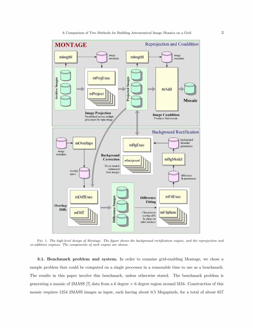
plane projections [4] (version 2) and the ability to run Montage in parallel (version 3). Figure 1 shows the
high level design for Montage, which is described in more detail in Table 1.
3. Grid-enabled Montage. In this section, we describe a benchmark problem and system, the ele-
ments needed to make this problem run on a grid using any approach, and the two approaches we have
studied. We then discuss the performance of the portions of the two approaches that differ, along with
advantages and disadvantages of each.
A Comparison of Two Methods for Building Astronomical Image Mosaics on a Grid 3
Fig. 1. The high-level design of Montage. The figure shows the background rectification engine, and the reprojection andco-addition engines. The components of each engine are shown.
3.1. Benchmark problem and system. In order to examine grid-enabling Montage, we chose a
sample problem that could be computed on a single processor in a reasonable time to use as a benchmark.
The results in this paper involve this benchmark, unless otherwise stated. The benchmark problem is
generating a mosaic of 2MASS [7] data from a 6 degree × 6 degree region around M16. Construction of this
mosaic requires 1254 2MASS images as input, each having about 0.5 Megapixels, for a total of about 657
4 Katz, D.S., et. al
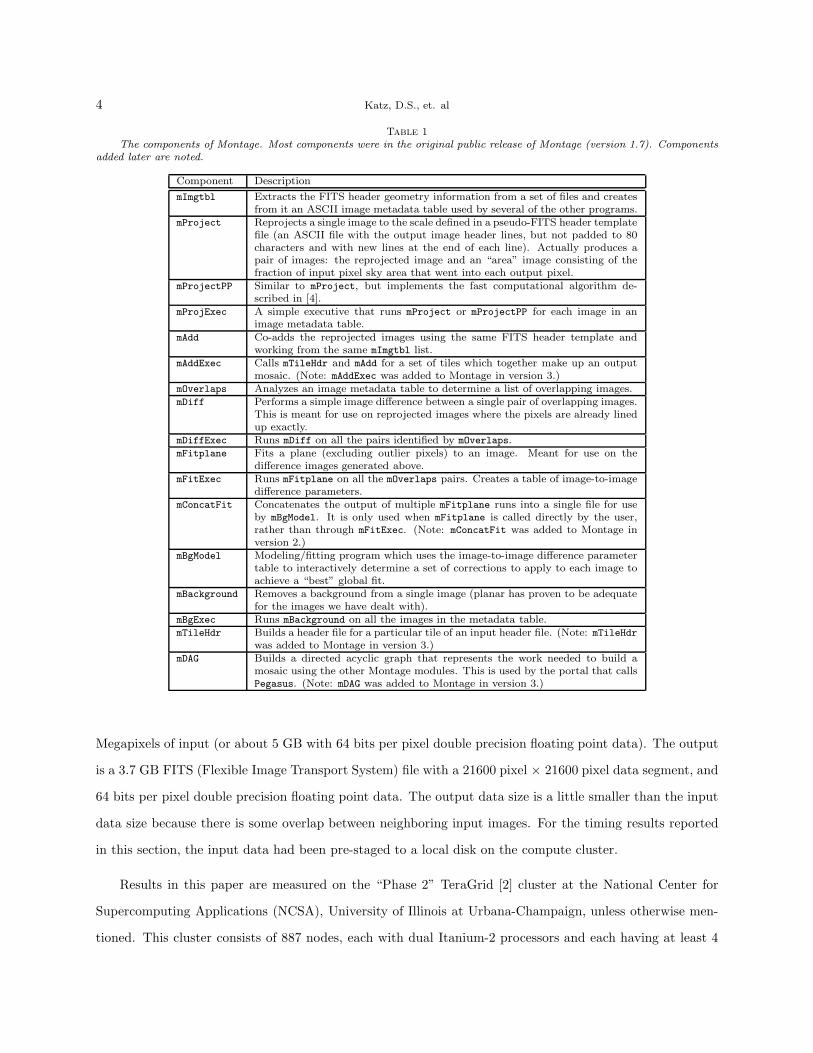
Table 1
The components of Montage. Most components were in the original public release of Montage (version 1.7). Componentsadded later are noted.
Component Description
mImgtbl Extracts the FITS header geometry information from a set of files and createsfrom it an ASCII image metadata table used by several of the other programs.
mProject Reprojects a single image to the scale defined in a pseudo-FITS header templatefile (an ASCII file with the output image header lines, but not padded to 80characters and with new lines at the end of each line). Actually produces apair of images: the reprojected image and an “area” image consisting of thefraction of input pixel sky area that went into each output pixel.
mProjectPP Similar to mProject, but implements the fast computational algorithm de-scribed in [4].
mProjExec A simple executive that runs mProject or mProjectPP for each image in animage metadata table.
mAdd Co-adds the reprojected images using the same FITS header template andworking from the same mImgtbl list.
mAddExec Calls mTileHdr and mAdd for a set of tiles which together make up an outputmosaic. (Note: mAddExec was added to Montage in version 3.)
mOverlaps Analyzes an image metadata table to determine a list of overlapping images.mDiff Performs a simple image difference between a single pair of overlapping images.
This is meant for use on reprojected images where the pixels are already linedup exactly.
mDiffExec Runs mDiff on all the pairs identified by mOverlaps.mFitplane Fits a plane (excluding outlier pixels) to an image. Meant for use on the
difference images generated above.mFitExec Runs mFitplane on all the mOverlaps pairs. Creates a table of image-to-image
difference parameters.mConcatFit Concatenates the output of multiple mFitplane runs into a single file for use
by mBgModel. It is only used when mFitplane is called directly by the user,rather than through mFitExec. (Note: mConcatFit was added to Montage inversion 2.)
mBgModel Modeling/fitting program which uses the image-to-image difference parametertable to interactively determine a set of corrections to apply to each image toachieve a “best” global fit.
mBackground Removes a background from a single image (planar has proven to be adequatefor the images we have dealt with).
mBgExec Runs mBackground on all the images in the metadata table.mTileHdr Builds a header file for a particular tile of an input header file. (Note: mTileHdr
was added to Montage in version 3.)mDAG Builds a directed acyclic graph that represents the work needed to build a
mosaic using the other Montage modules. This is used by the portal that callsPegasus. (Note: mDAG was added to Montage in version 3.)
Megapixels of input (or about 5 GB with 64 bits per pixel double precision floating point data). The output
is a 3.7 GB FITS (Flexible Image Transport System) file with a 21600 pixel × 21600 pixel data segment, and
64 bits per pixel double precision floating point data. The output data size is a little smaller than the input
data size because there is some overlap between neighboring input images. For the timing results reported
in this section, the input data had been pre-staged to a local disk on the compute cluster.
Results in this paper are measured on the “Phase 2” TeraGrid [2] cluster at the National Center for
Supercomputing Applications (NCSA), University of Illinois at Urbana-Champaign, unless otherwise men-
tioned. This cluster consists of 887 nodes, each with dual Itanium-2 processors and each having at least 4
A Comparison of Two Methods for Building Astronomical Image Mosaics on a Grid 5
GB of memory. 256 of the nodes have 1.3 GHz processors, and the other 631 nodes have 1.5 GHz processors.
The timing tests reported in this paper used the faster 1.5 GHz processors. The network interconnect be-
tween nodes is Myricom’s Myrinet and the operating system is SuSE Linux. Disk I/O is to a 24 TB General
Parallel File System (GPFS). Jobs are scheduled on the system using Portable Batch System (PBS) and the
queue wait time is not included in the execution times since that is heavily dependent on machine load from
other users.
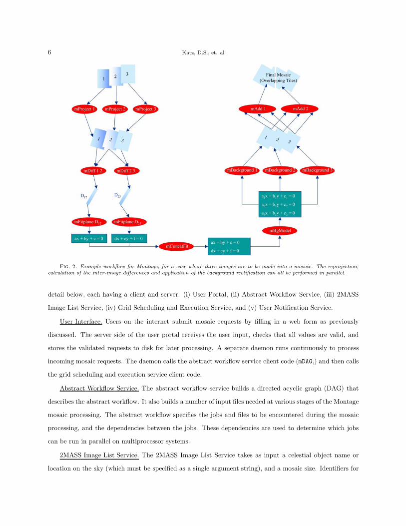
Figure 2 shows the processing steps for the benchmark problem. There are two types of parallelism:
simple file-based parallelism, and more complex module-based parallelism. Examples of file-based parallelism
are the mProject modules, each of which runs independently on a single file. mAddExec, which is used to
build an output mosaic in tiles, falls into this category as well, as once all the background-rectified files have
been built, each output tile may be constructed independently, except for I/O contention. The second type
of parallelism can be seen in mAdd, where any number of processors can work together to build a single output
mosaic. This module has been parallelized over blocks of rows of the output, but the parallel processes need
to be correctly choreographed to actually write the single output file. The results in this paper are for the
serial version of mAdd, where each output tile is constructed by a single processor.
3.2. Common grid features. The basic interface to Montage user is implemented as a web portal. In
this portal, the user selects a number of input parameters for the mosaicking job, such as the center and size
of the region of interest, the source of the data to be mosaicked, and some identification such as an email
address. Once this information is entered, the user assumes that the mosaic will be computed, and she will
be notified of the completion via an email message containing a URL where the mosaic can be retrieved.
Behind the scenes and hidden from the user’s view, a number of things have to happen to make this
work. First, a set of compute resources needs to be chosen. Here, we will assume that this is a cluster with
processors that have access to a shared file system. Second, the input data files and executable code needs
to be moved to these resources. Third, the modules need to be executed in the right order. In general, this
might involve moving intermediate files from one set of resources to another, but the previous assumption
makes this file movement unnecessary. Fourth, the output mosaic and perhaps some status information
needs to be moved to a location accessible to the user. Fifth and finally, the user must be notified of the job
completion and the location of the output(s).
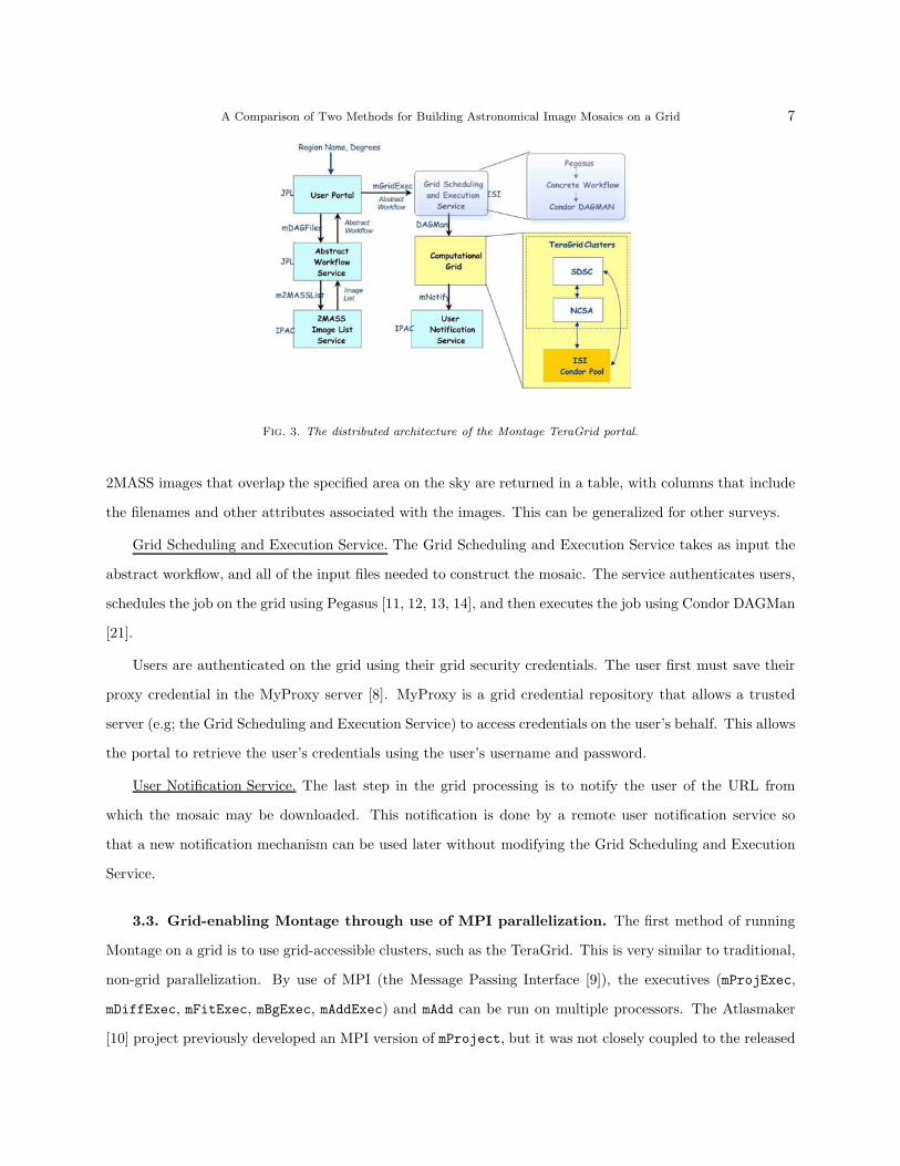
3.2.1. Montage portal. The Montage TeraGrid portal has a distributed architecture, as illustrated in
Figure 3. The initial version of portal is comprised of the following five main components, described in more
6 Katz, D.S., et. al
Fig. 2. Example workflow for Montage, for a case where three images are to be made into a mosaic. The reprojection,calculation of the inter-image differences and application of the background rectification can all be performed in parallel.
detail below, each having a client and server: (i) User Portal, (ii) Abstract Workflow Service, (iii) 2MASS
Image List Service, (iv) Grid Scheduling and Execution Service, and (v) User Notification Service.
User Interface. Users on the internet submit mosaic requests by filling in a web form as previously
discussed. The server side of the user portal receives the user input, checks that all values are valid, and
stores the validated requests to disk for later processing. A separate daemon runs continuously to process
incoming mosaic requests. The daemon calls the abstract workflow service client code (mDAG,) and then calls
the grid scheduling and execution service client code.
Abstract Workflow Service. The abstract workflow service builds a directed acyclic graph (DAG) that
describes the abstract workflow. It also builds a number of input files needed at various stages of the Montage
mosaic processing. The abstract workflow specifies the jobs and files to be encountered during the mosaic
processing, and the dependencies between the jobs. These dependencies are used to determine which jobs
can be run in parallel on multiprocessor systems.
2MASS Image List Service. The 2MASS Image List Service takes as input a celestial object name or
location on the sky (which must be specified as a single argument string), and a mosaic size. Identifiers for
A Comparison of Two Methods for Building Astronomical Image Mosaics on a Grid 7
Fig. 3. The distributed architecture of the Montage TeraGrid portal.
2MASS images that overlap the specified area on the sky are returned in a table, with columns that include
the filenames and other attributes associated with the images. This can be generalized for other surveys.
Grid Scheduling and Execution Service. The Grid Scheduling and Execution Service takes as input the
abstract workflow, and all of the input files needed to construct the mosaic. The service authenticates users,
schedules the job on the grid using Pegasus [11, 12, 13, 14], and then executes the job using Condor DAGMan
[21].
Users are authenticated on the grid using their grid security credentials. The user first must save their
proxy credential in the MyProxy server [8]. MyProxy is a grid credential repository that allows a trusted
server (e.g; the Grid Scheduling and Execution Service) to access credentials on the user’s behalf. This allows
the portal to retrieve the user’s credentials using the user’s username and password.
User Notification Service. The last step in the grid processing is to notify the user of the URL from
which the mosaic may be downloaded. This notification is done by a remote user notification service so
that a new notification mechanism can be used later without modifying the Grid Scheduling and Execution
Service.
3.3. Grid-enabling Montage through use of MPI parallelization. The first method of running
Montage on a grid is to use grid-accessible clusters, such as the TeraGrid. This is very similar to traditional,
non-grid parallelization. By use of MPI (the Message Passing Interface [9]), the executives (mProjExec,
mDiffExec, mFitExec, mBgExec, mAddExec) and mAdd can be run on multiple processors. The Atlasmaker
[10] project previously developed an MPI version of mProject, but it was not closely coupled to the released
8 Katz, D.S., et. al
Montage code, and therefore has not been maintained to work with current Montage releases. The current
MPI versions of the Montage modules are generated from the same source code as the single-processor
modules, by use of preprocessing directives.
The structure of the executives are similar to each other, in that each has some initialization that involves
determining a list of files on which a sub-module will be run, a loop in which the sub-module is actually
called for each file, and some finalization work that includes reporting on the results of the sub-module
runs. Additionally, two of the executives write to a log file after running each sub-module. The executives,
therefore, are parallelized very simply, with all processes of a given executive being identical to all the other
processes of that executive. All the initialization is duplicated by all processes. A line is added at the start
of the main loop, so that each process only calls the sub-module if the remainder of the loop count divided
by the number of processes equals the MPI rank (a logical identifier of an MPI process). All processes then
participate in global sums to find the total statistics of how many sub-modules succeeded, failed, etc., as
each process keeps track of its own statistics. After the global sums, only the process with rank 0 prints
the global statistics. For the two executives that write to a log file, the order of the entries in the log file
is unimportant. In these cases, each process writes to a unique temporary log file. Then, after the global
sums, the process with rank 0 runs an additional loop, where it reads lines from each process’s log file, then
writes them to a global log file, deleting each process’s temporary log file when done.
mAdd writes to the output mosaic one line at a time, reading from its input files as needed. The sequential
mAdd writes the FITS header information into the output file before starting the loop on output lines. In
the parallel mAdd, only the process with rank 0 writes the FITS header information, then it closes the file.
Now, each process can carefully seek and write to the correct part of the output file, without danger of
overwriting another process’s work. While the executives were written to divide the main loop operations in
a round-robin fashion, it makes more sense to parallelize the main mAdd loop by blocks, since it is likely that
a given row of the output file will depend on the same input files as the previous row, and this can reduce
the amount of input I/O for a given process.
Note that there are two modules that can be used to build the final output mosaic, mAdd and mAddExec,
and both can be parallelized as discussed in the previous two paragraphs. At this time, we have just run
one or the other, but it would be possible to combine them in a single run.
A set of system tests are available from the Montage web site. These tests, which consist of shell scripts
that call the various Montage modules in series, were designed for the single-processor version of Montage.
The MPI version of Montage is run similarly, by changing the appropriate lines of the shell script, for
A Comparison of Two Methods for Building Astronomical Image Mosaics on a Grid 9
example, from:
mProjExec arg1 arg2 ...
to:
mpirun -np N mProjExecMPI arg1 arg2 ...
These are the only changes that are needed. Notice that when this is run on a queuing system, some number
of processors will be reserved for the job. Some parts of the job, such as mImgtbl, will only use one processor,
and other parts, such as mProjExecMPI, will use all the processors. Overall, most of the processors are in
use most of the time. There is a small bit of overhead here in launching multiple MPI jobs on the same set
of processors. One might change the shell script into a parallel program, perhaps written in C or Python,
to avoid this overhead, but this has not been done for Montage.
A reasonable question to ask is how this approach differs from what might be done on a cluster that is
not part of a grid. The short answer to this somewhat rhetorical question is that the processing part of this
approach is not different. In fact, one might choose to run the MPI version of Montage on a local cluster
by logging in to the local cluster, transferring the input data to that machine, submitting a job that runs
the shell script to the queuing mechanism, and finally, after the job has run, retrieving the output mosaic.
Indeed, this is how the MPI code discussed in this paper was run and measured. The discussion of how
this code could be used in a portal is believed to be completely correct, but has not been implemented and
tested.
3.4. Grid-enabling Montage with Pegasus. Pegasus, which stands for Planning for Execution in
Grids, is a framework that enables the mapping of complex workflows onto distributed resources such as the
grid. In particular, Pegasus maps an abstract workflow to a form that can be executed on the grid using a
variety of computational platforms, from single hosts to Condor pools to compute clusters to the TeraGrid.
The Pegasus framework allows users to customize the type of resource and data selections performed as well
as to select the information sources. Pegasus was developed as part of the GriPhyN Virtual Data System
[15].
Abstract workflows describe the analysis in terms of logical transformations and data without identifying
the resources needed to execute the workflow. The abstract workflow for Montage consists of the various
application components shown in Figure 2. The nodes of the abstract workflow represent the logical trans-
formations such as mProject, mDiff and others. The edges represent the data dependencies between the
transformations. For example, mConcatFit requires all the files generated by all the previous mFitplane
10 Katz, D.S., et. al
steps.
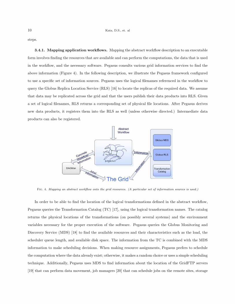
3.4.1. Mapping application workflows. Mapping the abstract workflow description to an executable
form involves finding the resources that are available and can perform the computations, the data that is used
in the workflow, and the necessary software. Pegasus consults various grid information services to find the
above information (Figure 4). In the following description, we illustrate the Pegasus framework configured
to use a specific set of information sources. Pegasus uses the logical filenames referenced in the workflow to
query the Globus Replica Location Service (RLS) [16] to locate the replicas of the required data. We assume
that data may be replicated across the grid and that the users publish their data products into RLS. Given
a set of logical filenames, RLS returns a corresponding set of physical file locations. After Pegasus derives
new data products, it registers them into the RLS as well (unless otherwise directed.) Intermediate data
products can also be registered.
Fig. 4. Mapping an abstract workflow onto the grid resources. (A particular set of information sources is used.)
In order to be able to find the location of the logical transformations defined in the abstract workflow,
Pegasus queries the Transformation Catalog (TC) [17], using the logical transformation names. The catalog
returns the physical locations of the transformations (on possibly several systems) and the environment
variables necessary for the proper execution of the software. Pegasus queries the Globus Monitoring and
Discovery Service (MDS) [18] to find the available resources and their characteristics such as the load, the
scheduler queue length, and available disk space. The information from the TC is combined with the MDS
information to make scheduling decisions. When making resource assignments, Pegasus prefers to schedule
the computation where the data already exist; otherwise, it makes a random choice or uses a simple scheduling
technique. Additionally, Pegasus uses MDS to find information about the location of the GridFTP servers
[19] that can perform data movement, job managers [20] that can schedule jobs on the remote sites, storage
A Comparison of Two Methods for Building Astronomical Image Mosaics on a Grid 11
locations, where data can be pre-staged, shared execution directories, the RLS into which new data can be
registered, site-wide environment variables, etc. This information is necessary to produce the submit files
that describe the necessary data movement, computation and catalog updates.
The information about the available data can be used to optimize the concrete workflow. If data products
described within the abstract workflow already exist, Pegasus can reuse them and thus reduce the complexity
of the concrete workflow. In general, the reduction component of Pegasus assumes that it is more costly
to execute a component (a job) than to access the results of the component if that data is available. For
example, some other user may have already materialized (made available on some storage system) part of
the entire required dataset. If this information is published into the RLS, Pegasus can utilize this knowledge
and obtain the data, thus avoiding possibly costly computation. As a result, some components that appear
in the abstract workflow do not appear in the concrete workflow.
Pegasus also checks for the feasibility of the abstract workflow. It determines the root nodes for the
abstract workflow and queries the RLS for the existence of the input files for these components. The workflow
can only be executed if the input files for these components can be found to exist somewhere on the grid
and are accessible via a data transport protocol.
The final result produced by Pegasus is an executable workflow that identifies the resources where the
computation will take place. In addition to the computational nodes, the concrete, executable workflow also
has data transfer nodes (for both stage-in and stage-out of data), data registration nodes that can update
various catalogs on the grid (for example, RLS), and nodes that can stage-in statically linked binaries.
3.4.2. Workflow execution. The concrete workflow produced by Pegasus is in the form of submit
files that are given to DAGMan and Condor-G for execution. The submit files indicate the operations to be
performed on given remote systems and the order in which the operations need to be performed. Given the
submit files, DAGMan submits jobs to Condor-G for execution. DAGMan is responsible for enforcing the
dependencies between the jobs defined in the concrete workflow.
In case of job failure, DAGMan can retry a job a given number of times. If that fails, DAGMan generates
a rescue workflow that can be potentially modified and resubmitted at a later time. Job retry is useful for
applications that are sensitive to environment or infrastructure instability. The rescue workflow is useful in
cases where the failure was due to lack of disk space that can be reclaimed or in cases where totally new
resources need to be assigned for execution. Obviously, it is not always beneficial to map and execute an
entire workflow at once, because resource availability may change over time. Therefore, Pegasus also has the
12 Katz, D.S., et. al
capability to map and then execute (using DAGMan) one or more portions of a workflow [14].
4. Comparison of approaches. In this section, we discuss the advantages and disadvantages of each
approach, as well as the performance of the two approaches, where there are differences in performance.
4.1. Starting the job. As discussed previously, we first need to choose a set of compute resources. In
both the MPI and Pegasus cases, the user can choose from a number of sets of resources. In the MPI case,
the user must choose a single set of processors that share a file system. In the Pegasus case, the user can
give Pegasus a set of resources to choose from, since transfer of files between processors can be automatically
handled by Pegasus. Pegasus is clearly more general. Here, so that we can compare performance, we use a
single set of processors on the TeraGrid cluster described previously as the benchmark system.
4.2. Data and code stage-in. Using either approach, the need for both data and code stage-in is
similar. The Pegasus approach has clear advantages, in that the Transformation Catalog can be used to
locate both code which has already been retrieved from archives as well as executables for a given machine.
Pegasus can use RLS to locate the input data. Once Pegasus locates the code and data, it can stage them
into an appropriate location. In the MPI approach, the user must know where the executable code is, which
is not a problem when the code is executed by the portal, as it then is the job of the portal creator. The
issue of reuse of data can also be handled by a local cache, though this is not as general as the use of RLS.
In any event, input data will sometimes need to be retrieved from an archive. In the initial version
of the portal discussed in this paper, we use the IPAC 2MASS list service, but in the future, we will use
the Simple Image Access Protocol (SIAP) [22], proposed by the International Virtual Observatory Alliance
(IVOA) [23]. SIAP can be used to obtain a table containing a list of files (URLs). One can then parse this
table, and actually retrieve the files.
Alternatively, a scientist may wish to work with data that is on her desktop. In this case, if using a
grid-enabled version of Montage, the user needs a mechanism for getting the data to the machine on which
the processing (or at least the first parts of it) will be done. Registering the data with RLS is a good solution
to this problem.
4.3. Building the mosaic. With the MPI approach, a job containing a shell script is submitted to
the queuing system. Each command in the script is either a sequential or parallel command to run a step
of the mosaic processing. The script will have some queue delay, then will start executing. Once it starts,
it runs until it finishes with no additional queue delays. The script itself would be generated by the portal.
It does not contain any detail on the actual data files, just the directories. The sequential commands in the
A Comparison of Two Methods for Building Astronomical Image Mosaics on a Grid 13
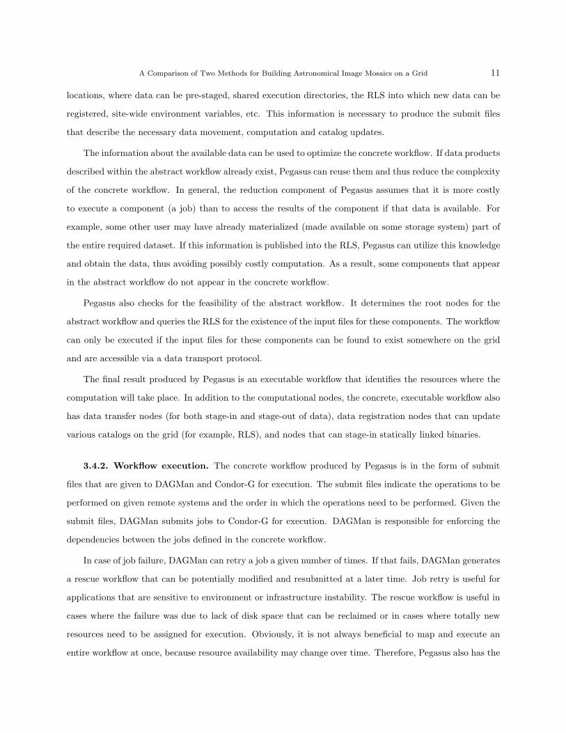
Table 2
Execution times (wallclock time in minutes) for a benchmark 2MASS mosaic, covering 6 degrees × 6 degrees centeredat M16, computed with Montage (version 2.1) on various numbers of 1.5 GHz processors of the NCSA TeraGrid cluster.Parallelization is done with MPI.
Number of Nodes (1 processor per node)Component 1 2 4 8 16 32 64
mImgtbl 0.7 1.05 1.05 1.2 1.4 1.3 1.2mProjExec (MPI) 142.3 68.0 34.1 17.2 8.8 4.8 3.07mImgtbl 1.1 1.0 0.9 1.3 1.1 1.2 1.2mOverlaps 0.05 0.05 0.05 0.05 0.05 0.05 0.05mDiffExec (MPI) 30.0 16.9 9.5 9.5 9.2 9.4 3.05mFitExec (MPI) 20.2 10.6 5.3 2.9 1.7 1.1 0.9mBgModel 1.1 1.1 1.1 1.1 1.1 1.1 1.1mBgExec (MPI) 11.3 6.0 3.8 2.6 2.3 2.6 2.6mImgtbl 1.05 0.9 0.9 1.1 1.1 1.2 1.2mAddExec (MPI) 245.5 124.5 63.1 40.6 24.1 18.4 11.3
Total 453.3 230.1 119.8 77.6 50.9 40.9 23.5
script examine the data directories and instruct the parallel jobs about the actual file names.
The Pegasus approach differs in that the initial work is quite a bit more complex, but the work done on
the compute nodes is much more simple. For reasons of efficiency, a pool of processors is allocated from the
parallel machine by use of the queuing system. Once this pool is available, Condor-Glidein [24] is used to
associate this pool with an existing Condor pool. Condor DAGMan then can fill the pool and keep it as full
as possible until all the jobs have been run. The decision about what needs to be run and in what order is
done by two parts of the portal. A module called mDAG builds the abstract DAG, and Pegasus then builds
the concrete DAG.
Because the queuing delays are one-time delays for both methods, we do not discuss them any further.
The elements for which we discuss timings below are the sequential and parallel jobs for the MPI approach,
and the mDAG, Pegasus, and compute modules for the Pegasus approach.
4.3.1. MPI timing results. The timing results of the MPI version of Montage are compiled in Table
2, which shows wall clock times in minutes for each Montage module run on the specified number of nodes
(with one processor per node) on the NCSA TeraGrid cluster. The end-to-end runs of Montage involved
running the modules in the order shown in the table. The modules that are parallelized are labeled as MPI;
all other modules are serial implementations. The execution times for the parallel modules on the different
numbers of cluster processors are plotted in Figure 5.
MPI parallelization reduces the one processor time of 453 minutes down to 23.5 minutes on 64 processors,
for a parallelization speedup of 19. Note that with the exception of some small initialization and finalization
code, all of the parallel code is non-sequential. The main reason the parallel modules fail to scale linearly as
the number of processors is increased is I/O. On a computer system with better parallel I/O performance,
14 Katz, D.S., et. al
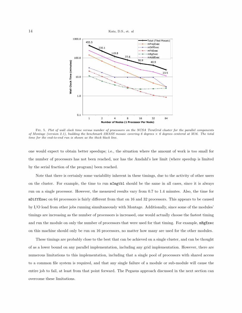
Fig. 5. Plot of wall clock time versus number of processors on the NCSA TeraGrid cluster for the parallel componentsof Montage (version 2.1), building the benchmark 2MASS mosaic covering 6 degrees × 6 degrees centered at M16. The totaltime for the end-to-end run is shown as the thick black line.
one would expect to obtain better speedups; i.e., the situation where the amount of work is too small for
the number of processors has not been reached, nor has the Amdahl’s law limit (where speedup is limited
by the serial fraction of the program) been reached.
Note that there is certainly some variability inherent in these timings, due to the activity of other users
on the cluster. For example, the time to run mImgtbl should be the same in all cases, since it is always
run on a single processor. However, the measured results vary from 0.7 to 1.4 minutes. Also, the time for
mDiffExec on 64 processors is fairly different from that on 16 and 32 processors. This appears to be caused
by I/O load from other jobs running simultaneously with Montage. Additionally, since some of the modules’
timings are increasing as the number of processors is increased, one would actually choose the fastest timing
and run the module on only the number of processors that were used for that timing. For example, mBgExec
on this machine should only be run on 16 processors, no matter how many are used for the other modules.
These timings are probably close to the best that can be achieved on a single cluster, and can be thought
of as a lower bound on any parallel implementation, including any grid implementation. However, there are
numerous limitations to this implementation, including that a single pool of processors with shared access
to a common file system is required, and that any single failure of a module or sub-module will cause the
entire job to fail, at least from that point forward. The Pegasus approach discussed in the next section can
overcome these limitations.
A Comparison of Two Methods for Building Astronomical Image Mosaics on a Grid 15
4.3.2. Pegasus timing results. When using remote grid resources for the execution of the concrete
workflow, there is a non-negligible overhead involved in acquiring resources and scheduling the computation
over them. In order to reduce this overhead, Pegasus can aggregate the nodes in the concrete workflow
into clusters so that the remote resources can be utilized more efficiently. The benefit of clustering is that
the scheduling overhead (from Condor-G, DAGMan and remote schedulers) is incurred only once for each
cluster. In the following results we cluster the nodes in the workflow within a workflow level (or workflow
depth). In the case of Montage, the mProject jobs are within a single level, mDiff jobs are in another level,
and so on. Clustering can be done dynamically based on the estimated run time of the jobs in the workflow
and the processor availability.
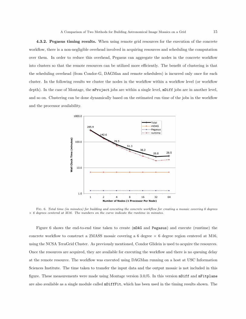
Fig. 6. Total time (in minutes) for building and executing the concrete workflow for creating a mosaic covering 6 degrees× 6 degrees centered at M16. The numbers on the curve indicate the runtime in minutes.
Figure 6 shows the end-to-end time taken to create (mDAG and Pegasus) and execute (runtime) the
concrete workflow to construct a 2MASS mosaic covering a 6 degree × 6 degree region centered at M16,
using the NCSA TeraGrid Cluster. As previously mentioned, Condor Glidein is used to acquire the resources.
Once the resources are acquired, they are available for executing the workflow and there is no queuing delay
at the remote resource. The workflow was executed using DAGMan running on a host at USC Information
Sciences Institute. The time taken to transfer the input data and the output mosaic is not included in this
figure. These measurements were made using Montage version 3.0β5. In this version mDiff and mFitplane
are also available as a single module called mDiffFit, which has been used in the timing results shown. The
16 Katz, D.S., et. al
figure shows the time taken in minutes for DAGMan to execute the workflow as the number of processors
are increased. The nodes in the workflow were clustered so that the number of clusters at each level of
the workflow was equal to the number of processors. As the number of processors is increased and thus
the number of clusters increases, the Condor overhead becomes the dominating factor. DAGMan takes
approximately 1 second to submit each cluster into the Condor queue. Condor’s scheduling overhead adds
additional delay. As a result we do not see a corresponding decrease in the workflow execution time as we
increase the number of processors. Also, as with the MPI results, the other codes running on the test machine
appear to impact these performance numbers. The 64 processor case seems to have worse performance than
the 32 processor case, but it is likely that were it rerun on a dedicated machine, it would have better
performance. This is discussed further in the next section. Finally, there are sequential sections in the
workflow that limit the overall parallel efficiency.
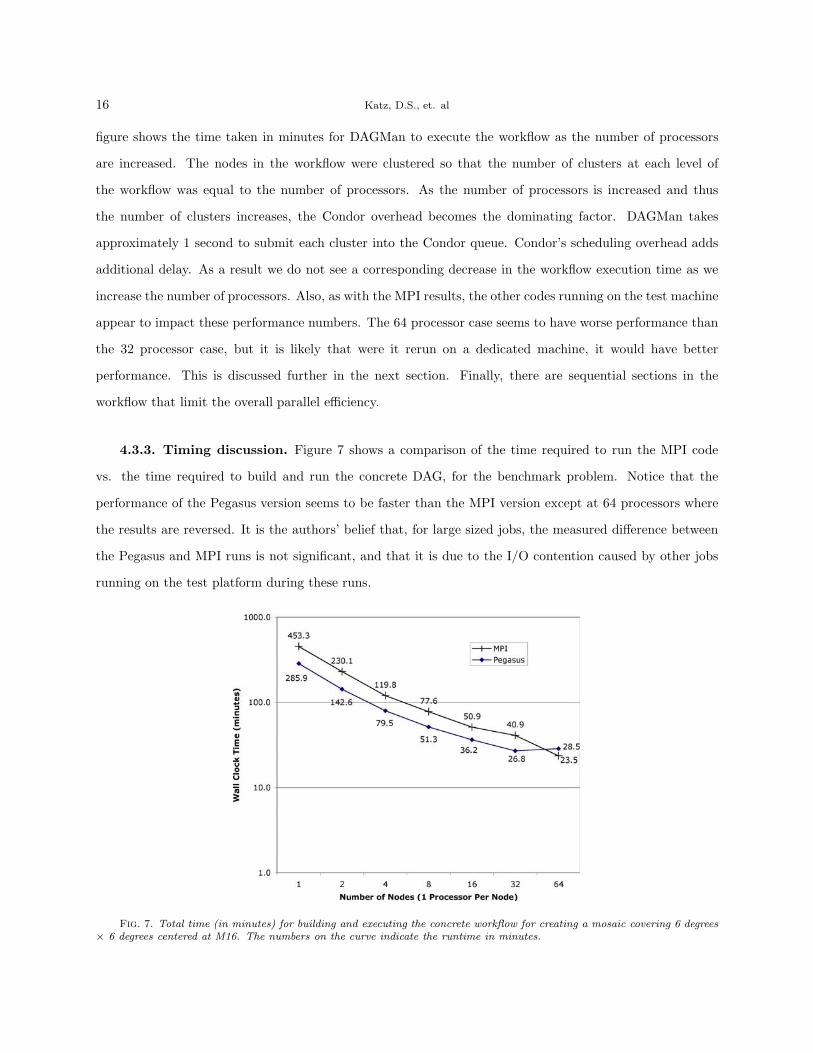
4.3.3. Timing discussion. Figure 7 shows a comparison of the time required to run the MPI code
vs. the time required to build and run the concrete DAG, for the benchmark problem. Notice that the
performance of the Pegasus version seems to be faster than the MPI version except at 64 processors where
the results are reversed. It is the authors’ belief that, for large sized jobs, the measured difference between
the Pegasus and MPI runs is not significant, and that it is due to the I/O contention caused by other jobs
running on the test platform during these runs.
Fig. 7. Total time (in minutes) for building and executing the concrete workflow for creating a mosaic covering 6 degrees× 6 degrees centered at M16. The numbers on the curve indicate the runtime in minutes.
A Comparison of Two Methods for Building Astronomical Image Mosaics on a Grid 17
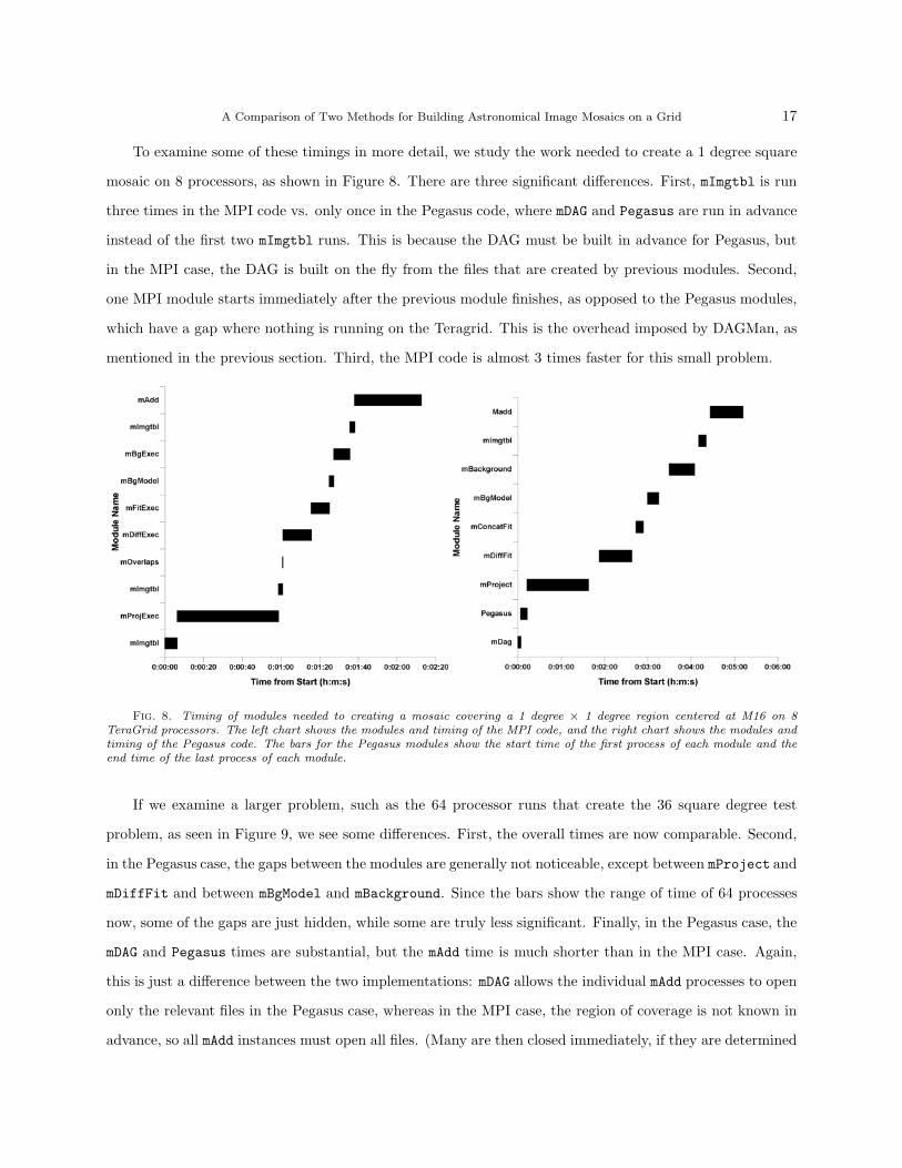
To examine some of these timings in more detail, we study the work needed to create a 1 degree square
mosaic on 8 processors, as shown in Figure 8. There are three significant differences. First, mImgtbl is run
three times in the MPI code vs. only once in the Pegasus code, where mDAG and Pegasus are run in advance
instead of the first two mImgtbl runs. This is because the DAG must be built in advance for Pegasus, but
in the MPI case, the DAG is built on the fly from the files that are created by previous modules. Second,
one MPI module starts immediately after the previous module finishes, as opposed to the Pegasus modules,
which have a gap where nothing is running on the Teragrid. This is the overhead imposed by DAGMan, as
mentioned in the previous section. Third, the MPI code is almost 3 times faster for this small problem.
Fig. 8. Timing of modules needed to creating a mosaic covering a 1 degree × 1 degree region centered at M16 on 8TeraGrid processors. The left chart shows the modules and timing of the MPI code, and the right chart shows the modules andtiming of the Pegasus code. The bars for the Pegasus modules show the start time of the first process of each module and theend time of the last process of each module.
If we examine a larger problem, such as the 64 processor runs that create the 36 square degree test
problem, as seen in Figure 9, we see some differences. First, the overall times are now comparable. Second,
in the Pegasus case, the gaps between the modules are generally not noticeable, except between mProject and
mDiffFit and between mBgModel and mBackground. Since the bars show the range of time of 64 processes
now, some of the gaps are just hidden, while some are truly less significant. Finally, in the Pegasus case, the
mDAG and Pegasus times are substantial, but the mAdd time is much shorter than in the MPI case. Again,
this is just a difference between the two implementations: mDAG allows the individual mAdd processes to open
only the relevant files in the Pegasus case, whereas in the MPI case, the region of coverage is not known in
advance, so all mAdd instances must open all files. (Many are then closed immediately, if they are determined
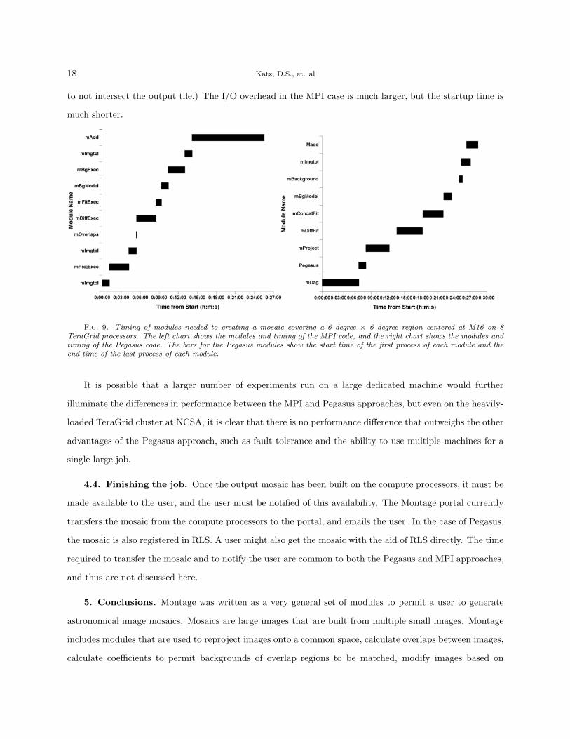
18 Katz, D.S., et. al
to not intersect the output tile.) The I/O overhead in the MPI case is much larger, but the startup time is
much shorter.
Fig. 9. Timing of modules needed to creating a mosaic covering a 6 degree × 6 degree region centered at M16 on 8TeraGrid processors. The left chart shows the modules and timing of the MPI code, and the right chart shows the modules andtiming of the Pegasus code. The bars for the Pegasus modules show the start time of the first process of each module and theend time of the last process of each module.
It is possible that a larger number of experiments run on a large dedicated machine would further
illuminate the differences in performance between the MPI and Pegasus approaches, but even on the heavily-
loaded TeraGrid cluster at NCSA, it is clear that there is no performance difference that outweighs the other
advantages of the Pegasus approach, such as fault tolerance and the ability to use multiple machines for a
single large job.
4.4. Finishing the job. Once the output mosaic has been built on the compute processors, it must be
made available to the user, and the user must be notified of this availability. The Montage portal currently
transfers the mosaic from the compute processors to the portal, and emails the user. In the case of Pegasus,
the mosaic is also registered in RLS. A user might also get the mosaic with the aid of RLS directly. The time
required to transfer the mosaic and to notify the user are common to both the Pegasus and MPI approaches,
and thus are not discussed here.
5. Conclusions. Montage was written as a very general set of modules to permit a user to generate
astronomical image mosaics. Mosaics are large images that are built from multiple small images. Montage
includes modules that are used to reproject images onto a common space, calculate overlaps between images,
calculate coefficients to permit backgrounds of overlap regions to be matched, modify images based on
A Comparison of Two Methods for Building Astronomical Image Mosaics on a Grid 19
those coefficients, and co-add images using a variety of methods of handling multiple pixels in the same
output space. The Montage modules can be run on a single processor computer using a simple shell script.
Because this approach can take a long time for a large mosaic, alternatives to make use of the grid have
been developed. The first alternative, using MPI versions of the computational intensive modules, has good
performance but is somewhat limited. A second alternative, using Pegasus and other grid tools, is more
general and allows for the execution on a variety of platforms without having to change the underlying code
base, and appears to have real-world performance comparable to that of the MPI approach for reasonably
large problems. Pegasus allows various scheduling techniques to be used to optimize the concrete workflow
for a particular execution platform. Other benefits of Pegasus include the ability to opportunistically take
advantage of available resources (through dynamic workflow mapping) and the ability to take advantage of
pre-existing intermediate data products, thus potentially improving the performance of the application.
6. Acknowledgments. The Pegasus software has been developed at the University of Southern Cal-
ifornia by Gaurang Mehta and Karan Vahi. We wish to thank Mr. Nathaniel Anagnostou for supporting
the Montage test effort. Use of TeraGrid resources for the work in this paper was supported by the National
Science Foundation under the following NSF programs: Partnerships for Advanced Computational Infras-
tructure, Distributed Terascale Facility (DTF), and Terascale Extensions: Enhancements to the Extensible
Terascale Facility.
REFERENCES
[1] The Montage project web page, http://montage.ipac.caltech.edu/
[2] The Distributed Terascale facility, http://www.teragrid.org/
[3] G. B. Berriman, D. Curkendall, J. C. Good, J. C. Jacob, D. S. Katz, M. Kong, S. Monkewitz, R. Moore, T. A.
Prince, and R. E. Williams, An architecture for access to a compute intensive image mosaic service in the NVO in
Virtual Observatories, A S. Szalay, ed., Proceedings of SPIE, v. 4846, 2002, pp. 91-102.
[4] G. B. Berriman, E. Deelman, J. C. Good, J. C. Jacob, D. S. Katz, C. Kesselman, A. C. Laity, T. A. Prince, G.
Singh, and M.-H. Su, Montage: A grid enabled engine for delivering custom science-grade mosaics on demand, in Op-
timizing Scientific Return for Astronomy through Information Technologies, P. J. Quinn, A. Bridger, eds., Proceedings
of SPIE, v. 5493, 2004, pp. 221-232.
[5] D. S. Katz, N. Anagnostou, G. B. Berriman, E. Deelman, J. Good, J. C. Jacob, C. Kesselman, A. Laity, T. A.
Prince, G. Singh, M.-H. Su, and R. Williams, Astronomical Image Mosaicking on a Grid: Initial Experiences, in
Engineering the Grid - Status and Perspective, B. Di Martino, J. Dongarra, A. Hoisie, L. Yang, and H. Zima, eds.,
Nova, expected 2005.
[6] Montage documentation and download, http://montage.ipac.caltech.edu/docs/
20 Katz, D.S., et. al
[7] The 2MASS Project, http://www.ipac.caltech.edu/2mass
[8] J. Novotny, S. Tuecke, and V. Welch, An online credential repository for the grid: MyProxy, in Proceedings of 10th
IEEE International Symposium on High Performance Distributed Computing, 2001.
[9] M. Snir, S. W. Otto, S. Huss-Lederman, D. W. Walker, and J. Dongarra, MPI: The Complete Reference, The MIT
Press, Cambridge, MA, 1996.
[10] R. D. Williams, S. G. Djorgovski, M. T. Feldmann, and J. C. Jacob, Atlasmaker: A grid-based implementation of
the hyperatlas, Astronomical Data Analysis Software & Systems (ADASS) XIII, 2003.
[11] E. Deelman, S. Koranda, C. Kesselman, G. Mehta, L. Meshkat, L. Pearlman, K. Blackburn, P. Ehrens, A.
Lazzarini, and R. Williams, GriPhyN and LIGO, building a virtual data grid for gravitational wave scientists, in
Proceedings of 11th IEEE International Symposium on High Performance Distributed Computing, 2002.
[12] E. Deelman, J. Blythe, Y. Gil, C. Kesselman, G. Mehta, and K. Vahi, Mapping abstract complex workflows onto
grid environments, Journal of Grid Computing, v. 1(1), 2003.
[13] E. Deelman, R. Plante, C. Kesselman, G. Singh, M.-H. Su, G. Greene, R. Hanisch, N. Gaffney, A. Volpicelli, J.
Annis, V. Sekhri, T. Budavari, M. Nieto-Santisteban, W. OMullane, D. Bohlender, T. McGlynn, A. Rots,
and O. Pevunova, Grid-based galaxy morphology analysis for the national virtual observatory, in Proceedings of
SC2003, 2003.
[14] E. Deelman, J. Blythe, Y. Gil, C. Kesselman, G. Mehta, S. Patil, M.-H. Su, K. Vahi, and M. Livny, Pegasus:
mapping scientific workflows onto the grid, in Across Grids Conference 2004.
[15] GriPhyN, http://www.griphyn.org/
[16] A. Chervenak, E. Deelman, I. Foster, L. Guy, W. Hoschek, A. Iamnitchi, C. Kesselman, P. Kunst, M. Ripeanu,
B. Schwartzkopf, H. Stockinger, K. Stockinger, and B. Tierney, Giggle: a framework for constructing scalable
replica location services, in Proceedings of SC2002, 2002.
[17] E. Deelman, C. Kesselman, and G. Mehta, Transformation catalog design for GriPhyN, GriPhyN Technical Report
2001-17, 2001.
[18] K. Czajkowski, S. Fitzgerald, I. Foster, and C. Kesselman, Grid information services for distributed resource sharing,
in Proceedings of the 10th IEEE Symposium on High-Performance Distributed Computing, 2001.
[19] B. Allcock, S. Tuecke, J. Bester, J. Bresnahan, A. L. Chervenak, I. Foster, C. Kesselman, S. Meder, V.
Nefedova, and D. Quesnel, Data management and transfer in high performance computational grid environments,
Parallel Computing, v. 28(5), 2002, pp. 749-771.
[20] K. Czajkowski, A. K. Demir, C. Kesselman, and M. Thiebaux, Practical resource management for grid-based visual
exploration, in Proceedings of the 10th IEEE Symposium on High-Performance Distributed Computing, 2001.
[21] J. Frey, T. Tannenbaum, M. Livny, and S. Tuecke, Condor-G: a computation management agent for multi-institutional
grids, in Proceedings of the 10th IEEE Symposium on High-Performance Distributed Computing, 2001.
[22] D. Tody, R. Plante, Simple image access specification version 1.0, http://www.ivoa.net/Documents/latest/SIA.html
[23] International Virtual Observatory Alliance, http://www.ivoa.net/
[24] Condor-Glidein, http://www.cs.wisc.edu/condor/glidein