A comparison of performance of several artificial intelligence

Journal of Hydrology, Vol. 374, No. 3-4, 2009, pp 294–306

1

A comparison of performance of several artificial intelligence 1

methods for forecasting monthly discharge time series 2

3

Wen-Chuan Wang 4

Ph.D., Institute of hydropower system & Hydroinformatics, Dalian University of Technology, 5 Dalian, 116024, P.R. China 6

Faculty of Water conservancy Engineering, North China Institute of Water Conservancy and 7 Hydroelectric Power, Zhengzhou 450011, P.R.China 8 9 Kwok-Wing Chau 10 Associate Professor, Department of Civil and Structural Engineering, Hong Kong Polytechnic 11

University, Hung Hom, Kowloon, Hong Kong (Corresponding author): E-mail address: 12

[email protected] Tel.: (+852) 2766 6014 13

14

Chun-Tian Cheng 15

Professor, Institute of hydropower system & Hydroinformatics, Dalian University of Technology, 16 Dalian, 116024, P.R. China 17

18

Lin Qiu 19

Professor, Institute of environmental & municipal engineering, North China Institute of Water 20

Conservancy and Hydroelectric power, ZhengZhou, 450011, P.R.Ch 21

22

Abstract. Developing a hydrological forecasting model based on past records is crucial to 23

effective hydropower reservoir management and scheduling. Traditionally, time series analysis and 24

modeling is used for building mathematical models to generate hydrologic records in hydrology 25

and water resources. Artificial intelligence (AI), as a branch of computer science, is capable of 26

analyzing long-series and large-scale hydrological data. In recent years, it is one of front issues to 27

apply AI technology to the hydrological forecasting modeling. In this paper, autoregressive 28

moving-average (ARMA) models, artificial neural networks (ANNs) approaches, adaptive 29

neural-based fuzzy inference system (ANFIS) techniques, genetic programming (GP) models and 30

support vector machine (SVM) method are examined using the long-term observations of monthly 31

river flow discharges. The four quantitative standard statistical performance evaluation measures, 32

the coefficient of correlation (R), Nash-Sutcliffe efficiency coefficient (E), root mean squared 33

error (RMSE), mean absolute percentage error (MAPE), are employed to evaluate the 34

performances of various models developed. Two case study river sites are also provided to 35

illustrate their respective performances. The results indicate that the best performance can be 36

obtained by ANFIS, GP and SVM, in terms of different evaluation criteria during the training and 37

validation phases. 38

39

Key words: monthly discharge time series forecasting; ARMA; ANN; ANFIS; GP; SVM 40

41

This is the Pre-Published Version.


2

1. Introduction 42

The identification of suitable models for forecasting future monthly inflows to hydropower 43

reservoirs is a significant precondition for effective reservoir management and scheduling. The 44

results, especially in long-term prediction, are useful in many water resources applications such as 45

environment protection, drought management, operation of water supply utilities, optimal 46

reservoir operation involving multiple objectives of irrigation, hydropower generation, and 47

sustainable development of water resources, etc. As such, hydrologic time series forecasting has 48

always been of particular interest in operational hydrology. It has received tremendous attention of 49

researchers in last few decades and many models for hydrologic time series forecasting have been 50

proposed to improve the hydrology forecasting. 51

These models can be broadly divided into three groups: regression based methods, time series 52

models and AI-based methods. For autoregressive moving-average models (ARMA) proposed by 53

Box and Jenkins (1970), it is assumed that the times series is stationary and follows the normal 54

distribution. ARMA is one of the most popular hydrologic times series models for reservoir design 55

and optimization. Extensive application and reviews of the several classes of such models 56

proposed for the modelling of water resources time series were reported (Chen and Rao, 2002; 57

Salas, 1993; Srikanthan and McMahon, 2001). 58

In recent years, AI technique, being capable of analysing long-series and large-scale data, 59

has become increasingly popular in hydrology and water resources among researchers and 60

practicing engineers. Since the 1990s, artificial neural networks (ANNs), based on the 61

understanding of the brain and nervous systems, was gradually used in hydrological prediction. An 62

extensive review of their use in the hydrological field is given by ASCE Task Committee on 63

Application of Artificial Neural Networks in Hydrology (ASCE, 2000a; ASCE, 2000b).The ANNs 64

have been shown to give useful results in many fields of hydrology and water resources research 65

(Campolo et al., 2003; Chau, 2006; Muttil and Chau, 2006). 66

The adaptive neural-based fuzzy inference system (ANFIS) model and its principles, first 67

developed by Jang (1993), have been applied to study many problems and also in hydrology field 68

as well. Chang & Chang (2001) studied the integration of a neural network and fuzzy arithmetic 69

for real-time streamflow forecasting and reported that ANFIS helps to ensure more efficient 70

reservoir operation than the classical models based on rule curve. Bazartseren et al. (2003) used 71

neuro-fuzzy and neural network models for short-term water level prediction. Dixon (2005) 72

examined the sensitivity of neuron-fuzzy models used to predict groundwater vulnerability in a 73

spatial context by integrating GIS and neuro-fuzzy techniques. Other researchers reported good 74

results in applying ANFIS in hydrological prediction (Cheng et al., 2005; Keskin et al., 2006; 75

Nayak et al., 2004). 76

Genetic Programming (GP), an extension of the well known field of genetic algorithms (GA) 77

belonging to the family of evolutionary computation, is an automatic programming technique for 78

evolving computer programs to solve problems (Koza, 1992). GP model was used to emulate the 79

rainfall-runoff process (Whigam and Crapper, 2001) and was evaluated in terms of root mean 80

square error and correlation coefficient (Liong et al., 2002; Whigam and Crapper, 2001). It was 81

shown to be a viable alternative to traditional rainfall runoff models. The GP approach was also 82

employed by Johari et al (2006) to predict the soil-water characteristic curve of soils. GP is 83

employed for modelling and prediction of algal blooms in Tolo Harbour, Hong Kong (Muttil and 84


3

Chau, 2006) and the results indicated good predictions of long-term trends in algal biomass. The 85

Darwinian theory-based GP approach was suggested for improving fortnightly flow forecast for a 86

short time-series (Sivapragasam et al., 2007). 87

The support vector machine (SVM) is based on structural risk minimization (SRM) principle 88

and is an approximation implementation of the method of SRM with a good generalisation 89

capability (Vapnik, 1998). Although SVM has been used in applications for a relatively short time, 90

this learning machine has been proven to be a robust and competent algorithm for both 91

classification and regression in many disciplines. Recently, the use of the SVM in water resources 92

engineering has attracted much attention. Dibike et al. (2001) demonstrated its use in rainfall 93

runoff modeling. Liong and Sivapragasam (2002) applied SVM to flood stage forecasting in 94

Dhaka, Bangladesh and concluded that the accuracy of SVM exceeded that of ANN in 95

one-lead-day to seven-lead-day forecasting. Yu et al.(2006) successfully explored the usefulness of 96

SVM based modelling technique for predicting of real time flood stage forecasting on Lan-Yang 97

river in Taiwan 1 to 6 hours ahead. Khan and Coulibaly (2006) demonstrated the application of 98

SVM to time series modeling in water resources engineering for lake water level prediction. The 99

SVM method has also been employed for stream flow predictions (Asefa et al., 2006; Lin et al., 100

2006). 101

The major objectives of the study presented in this paper are to investigate several AI 102

techniques for modelling monthly discharge time series, which include ANN approaches, ANFIS 103

techniques, GP models and SVM method, and to compare their performance with other traditional 104

time series modelling techniques such as ARMA. Four quantitative standard statistical 105

performance evaluation measures, i.e., coefficient of correlation (R), Nash-Sutcliffe efficiency 106

coefficient (E), root mean squared error (RMSE), mean absolute percentage error (MAPE), are 107

employed to validate all models. Brief introduction and model development of these AI methods 108

are also described before discussing the results and making concluding remarks. The performances 109

of various models developed are demonstrated by forecasting monthly river flow discharges in 110

Manwan Hydropower and Hongjiadu Hydropower. 111

2 Description of Selected Models 112

Several AI techniques employed in this study include ANNs, ANFIS techniques, GP models and 113

SVM method. A brief overview of these techniques is presented here. 114

2.1 Artificial Neural Networks (ANNs) 115

Since early 1990s, ANNs, and in particular, feed-forward back-propagation perceptrons have been 116

used for forecasting in many areas of science and engineering (Chau and Cheng, 2002). An ANN 117

is an information processing system composed of many nonlinear and densely interconnected 118

processing elements or neurons, which is organized as layers connected via weights between 119

layers. An ANN usually consists of three layers: the input layer, where the data are introduced to 120

the network; the hidden layer or layers, where data are processed; and the output layer, where the 121

results of given input are produced. The structure of a feed-forward ANN is shown in Fig. 1. 122

A multi-layer feed-forward back-propagation network with one hidden layer has been used 123


4

throughout the study (Haykin, 1999). In a feed-forward back-propagation network, the weighted 124

connections feed activations only in the forward direction from an input layer to the output layer. 125

These interconnections are adjusted using an error convergence technique so that the network’s 126

response best matches the desired response. The main advantage of the ANN technique over 127

traditional methods is that it does not require information about the complex nature of the 128

underlying process under consideration to be explicitly described in mathematical form. 129

2.2 Adaptive neural-based fuzzy inference system (ANFIS) 130

The ANFIS used in the study is a fuzzy inference model of Sugeno type, and is a 131

composition of ANNs and fuzzy logic approaches (Jang, 1993; Jang et al., 1997). The model 132

identifies a set of parameters through a hybrid learning rule combining the back-propagation 133

gradient descent and a least squares method. It can be used as a basis for constructing a set of 134

fuzzy IF-THEN rules with appropriate membership functions in order to generate the previously 135

stipulated input-output pairs (Keskin et al., 2006). 136

The Sugeno fuzzy inference system is computationally efficient and works well with linear 137

techniques, optimization and adaptive techniques. As a simple example, we assume a fuzzy 138

inference system with two inputs x and y and one output z. The first-order Sugeno fuzzy model, a 139

typical rule set with two fuzzy If-Then rules can be expressed as: 140

Rule 1:If x is A1 and y is B1，then 1111 ryqxpf 141

Rule 2:If x is A2 and y is B2，then 2222 ryqxpf 142

The resulting Sugeno fuzzy reasoning system is shown in Fig. 2. It illustrates the fuzzy 143

reasoning mechanism for this Sugeno model to derive an output function (f) from a given input 144

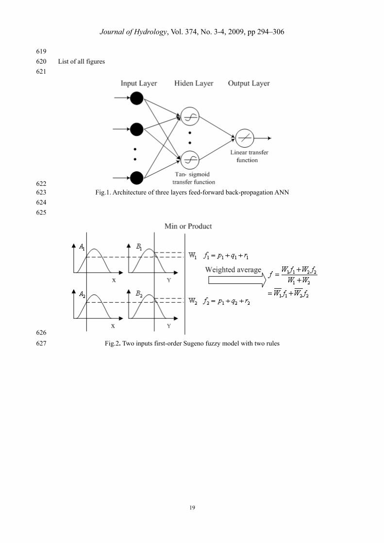
vector [x, y]. The corresponding equivalent ANFIS architecture is a five-layer feed forward net 145

work that uses neural net work learning algorithms coupled with fuzzy reasoning to map an input 146

space to an output space. It is shown in Fig.3. The more comprehensive presentation of ANFIS for 147

forecasting hydrological time series can be found in the literature (Cheng et al., 2005; Keskin et al., 148

2006; Nayak et al., 2004). 149

2.3 Genetic programming (GP) 150

GP is a search methodology belonging to the class of ‘intelligent’ methods which allows the 151

solution of problems by automatically generating algorithms and expressions. These expressions 152

are codified or represented as a tree structure with its terminals (leaves) and nodes (functions). GP, 153

similar to GA, initializes a population that compounds the random members known as 154

chromosomes (individual). Afterward, fitness of each chromosome is evaluated with respect to a 155

target value. GP works with a number of solution sets, known collectively as a “population”, 156

rather than a single solution at any one time; the possibility of getting trapped in a “local 157

optimum” is thus avoided. GP differs from the traditional GA in that it typically operates on parse 158

trees instead of bit strings. A parse tree is built up from a terminal set (the variables in the problem) 159

and a function set (the basic operators used to form the function). GP is provided with evaluation 160

data, a set of primitives and fitness functions. The evaluation data describe the specific problem in 161


5

terms of the desired inputs and outputs. They are used to generate the best computer program to 162

describe the relationship between the input and output very well (Koza, 1992). 163

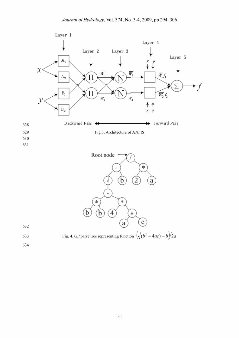
The representation of GP can be viewed as a parse tree-based structure composed of the 164

function set and terminal set. The function set is the operators, functions or statements such as 165

arithmetic operators ({+, -, *, /}) or conditional statements (if… then…) which are available in the 166

GP. The terminal set contains all inputs, constants and other zero-argument in the GP tree. An 167

example of such a parse tree can be found in Fig. 4. Once a population of the GP tree is initialized, 168

the following procedures are similar to GAs including defining the fitness function, genetic 169

operators such as crossover, mutation and reproduction and the termination criterion, etc. In GP, 170

the crossover operator is used to swap the subtree from the parents to reproduce the children using 171

mating selection policy rather than exchanging bit strings as in GAs. 172

The genetic programming introduced here is one of the simplest forms available. A more 173

comprehensive presentation of GP can be found in the literature (Borrelli et al., 2006; Koza, 174

1992). 175

2.4 Support vector machine (SVM) 176

SVM is the state-of-the-art neural network technology based on statistical learning (Vapnik, 1995; 177

Vapnik, 1998). The basic idea of SVM is to use linear model to implement nonlinear class 178

boundaries through some nonlinear mapping of the input vector into the high-dimensional feature 179

space. The linear model constructed in the new space can represent a nonlinear decision boundary 180

in the original space. In the new space, SVM constructs an optimal separating hyperplane. If the 181

data is linearly separated, linear machines are trained for an optimal hyperplane that separates the 182

data without error and into the maximum distance between the hyperplane and the closest training 183

points. The training points that are closest to the optimal separating hyperplane are called support 184

vectors. Fig. 5 exhibits the basic concept of SVM. There exist uncountable decision functions, i.e. 185

hyperplanes, which can effectively separate the negative and positive data set (denoted by ‘x’ and 186

‘o’, respectively) that has the maximal margin. This indicates that the distance from the closest 187

positive samples to a hyperplane and the distance from the closest negative samples to it will be 188

maximized. 189

Given a set of training data Niii dx )},{( (xi is the input vector, di is the desired value and N is the 190

total number of data patterns), the regression function of SVM is formulated as follows: 191

bxwxfy ii )()( (1) 192

where )(xi is the feature of inputs, and iw and b are coefficients. The coefficients 193 ( iw and b) are estimated by minimizing the following regularized risk function (Vapnik, 194 1995; Vapnik, 1998): 195

2

1

||||2

1),(

1)(

ii

N

i

ydLN

CCr (2) 196

where 197

0

||),(

ydydL

otherwise

ydif || (3) 198


6

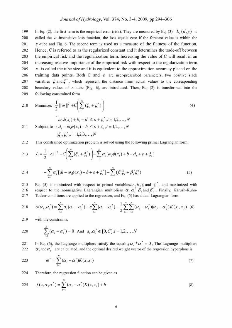
In Eq. (2), the first term is the empirical error (risk). They are measured by Eq. (3). ),( ydL is 199

called the -insensitive loss function, the loss equals zero if the forecast value is within the 200

-tube and Fig. 6. The second term is used as a measure of the flatness of the function, 201

Hence, C is referred to as the regularized constant and it determines the trade-off between 202

the empirical risk and the regularization term. Increasing the value of C will result in an 203

increasing relative importance of the empirical risk with respect to the regularization term. 204

is called the tube size and it is equivalent to the approximation accuracy placed on the 205

training data points. Both C and are user-prescribed parameters, two positive slack 206

variables and * , which represent the distance from actual values to the corresponding 207

boundary values of -tube (Fig. 6), are introduced. Then, Eq. (2) is transformed into the 208

following constrained form. 209

Minimize:

N

iiiC )(||||

2

1 *2 (4) 210

Subject to

Ni

Nibxd

Nidbx

ii

iiiii

iiiii

,,3,2,1,,

,,2,1,)(

,,2,1,)(

*

*

211

This constrained optimization problem is solved using the following primal Lagrangian form: 212

N

iiiiii

N

iii dbxCL ])([)(||||

2

1 *2 213

N

i

iiiiiiii

N

ii bxdi )(])([ **

1

* (5) 214

Eq. (5) is minimized with respect to primal variables i , b , and * , and maximized with 215 respect to the nonnegative Lagrangian multipliers i

*i i and *

i , Finally, Karush-Kuhn- 216 Tucker conditions are applied to the regression, and Eq. (5) has a dual Lagrangian form: 217

),())((2

1)()(),( *

1 1

*

1

**

1

*jijj

N

i

N

iii

N

iiiii

N

iiii xxKd

(6) 218

with the constraints, 219

0)(1

*

N

iii And NiCa ii ,,2,1],,0[, * 220

In Eq. (6), the Lagrange multipliers satisfy the equality 0* * ii , The Lagrange multipliers 221

i and *i are calculated, and the optimal desired weight vector of the regression hyperplane is 222

),()(1

*i

N

i

iii xxK

(7) 223

Therefore, the regression function can be given as 224

bxxKxf i

N

iii

),()(),,(1

** (8) 225


7

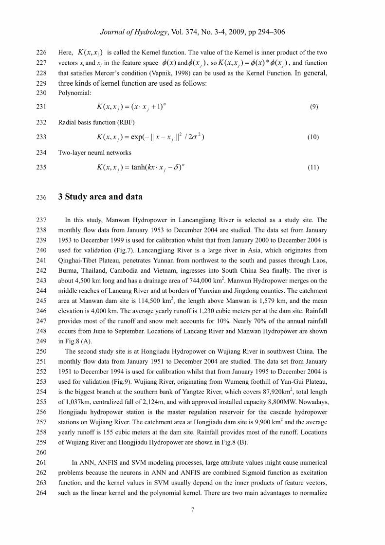
Here, ),( ixxK is called the Kernel function. The value of the Kernel is inner product of the two 226

vectors xi and xj in the feature space )(x and )( jx , so )(*)(),( jj xxxxK , and function 227

that satisfies Mercer’s condition (Vapnik, 1998) can be used as the Kernel Function. In general, 228

three kinds of kernel function are used as follows: 229 Polynomial: 230

njj xxxxK )1(),( (9) 231

Radial basis function (RBF) 232

)2/||||exp(),( 22 jj xxxxK (10) 233

Two-layer neural networks 234

njj xkxxxK )tanh(),( (11) 235

3 Study area and data 236

In this study, Manwan Hydropower in Lancangjiang River is selected as a study site. The 237

monthly flow data from January 1953 to December 2004 are studied. The data set from January 238

1953 to December 1999 is used for calibration whilst that from January 2000 to December 2004 is 239

used for validation (Fig.7). Lancangjiang River is a large river in Asia, which originates from 240

Qinghai-Tibet Plateau, penetrates Yunnan from northwest to the south and passes through Laos, 241

Burma, Thailand, Cambodia and Vietnam, ingresses into South China Sea finally. The river is 242

about 4,500 km long and has a drainage area of 744,000 km2. Manwan Hydropower merges on the 243

middle reaches of Lancang River and at borders of Yunxian and Jingdong counties. The catchment 244

area at Manwan dam site is 114,500 km2, the length above Manwan is 1,579 km, and the mean 245

elevation is 4,000 km. The average yearly runoff is 1,230 cubic meters per at the dam site. Rainfall 246

provides most of the runoff and snow melt accounts for 10%. Nearly 70% of the annual rainfall 247

occurs from June to September. Locations of Lancang River and Manwan Hydropower are shown 248

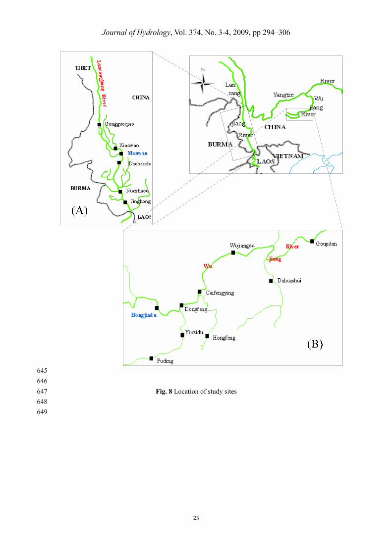
in Fig.8 (A). 249

The second study site is at Hongjiadu Hydropower on Wujiang River in southwest China. The 250

monthly flow data from January 1951 to December 2004 are studied. The data set from January 251

1951 to December 1994 is used for calibration whilst that from January 1995 to December 2004 is 252

used for validation (Fig.9). Wujiang River, originating from Wumeng foothill of Yun-Gui Plateau, 253

is the biggest branch at the southern bank of Yangtze River, which covers 87,920km2, total length 254

of 1,037km, centralized fall of 2,124m, and with approved installed capacity 8,800MW. Nowadays, 255

Hongjiadu hydropower station is the master regulation reservoir for the cascade hydropower 256

stations on Wujiang River. The catchment area at Hongjiadu dam site is 9,900 km2 and the average 257

yearly runoff is 155 cubic meters at the dam site. Rainfall provides most of the runoff. Locations 258

of Wujiang River and Hongjiadu Hydropower are shown in Fig.8 (B). 259

260

In ANN, ANFIS and SVM modeling processes, large attribute values might cause numerical 261

problems because the neurons in ANN and ANFIS are combined Sigmoid function as excitation 262

function, and the kernel values in SVM usually depend on the inner products of feature vectors, 263

such as the linear kernel and the polynomial kernel. There are two main advantages to normalize 264


8

features before applying ANN, ANFIS and SVM to prediction. One advantage is to avoid 265

attributes in greater numeric ranges dominating those in smaller numeric ranges, and another 266

advantage is to avoid numerical difficulties during the calculation. It is recommended to linearly 267

scale each attribute to the range [-1, +1] or [0, 1]. In the modeling process, the data sets of river 268

flow were scaled to the range between 0 and 1 as follow: 269

min

min'

qq

qqq

maz

ii

(12) 270

where 'iq is the scaled value, iq is the original flow value and minq , mazq are respectively 271

the minimum and maximum of flow series. 272

4. Prediction modeling and input selection 273

We are interested in hydrological forecasting model that predict outputs from inputs based on 274

past records. There are no fixed rules for developing these AI techniques (ANN, ANFIS, GP, 275

SVM), even though a general framework can be followed based on previous successful 276

applications in engineering (Cheng et al., 2005; Lin et al., 2006; Nayak et al., 2004; Sudheer et al., 277

2002). The objective of studies focus on predicting discharges using antecedent values is to 278

generalize a relationship of the following form: 279

)( mXfY (13) 280

where Xm is a m-dimensional input vector consisting of variables x1,…,xi,…xm, and Y is the output 281

variable. In discharge modeling, values of xi may be flow values with different time lags and the 282

value Y is generally the flow in the next period. Generally, the number of antecedent values 283

included in the vector Xm is not known a priori. 284

In these AI techniques, being typical in any data-driven prediction models, the selection of 285

appropriate model input vector would play an important role in their successful implementation 286

since it provides the basic information about the system being modeled. The parameters 287

determined as input variables are the numbers of flow values for finding the lags of runoff that 288

have a significant influence on the predicted flow. These influencing values corresponding to 289

different lags can be very well established through a statistical analysis of the data series. 290

Statistical procedures were suggested for identifying an appropriate input vector for a model (Lin 291

et al., 2006; Sudheer et al., 2002). In this study, two statistical methods (i.e. the autocorrelation 292

function (ACF) and the partial autocorrelation function (PACF)) are employed to determine the 293

number of parameters corresponding to different antecedents values. The influencing antecedent 294

discharge patterns can be suggested by the ACF and PACF in the flow at a given time. The ACF 295

and PACF are generally used in diagnosing the order of the autoregressive process and can also be 296

employed in prediction modeling (Lin et al., 2006). The values of ACF and PACF of monthly flow 297

sequence (1953/1~1999/12) is calculated for lag 0 to 24 in Manwan, which are presented in Fig.10. 298

Similarly, the values of ACF and PACF of monthly flow sequence (1951/1~1994/12) is calculated 299

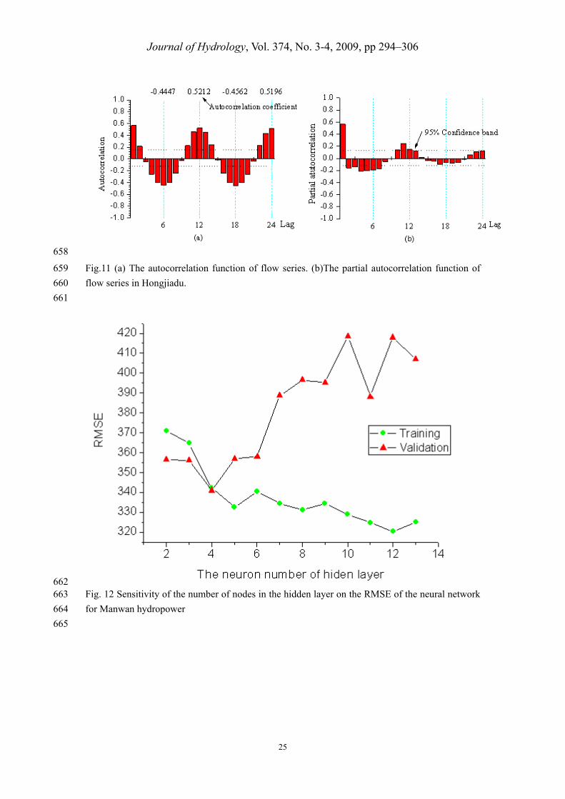
for lag 0 to 24 in Hongjiadu, which are presented in Fig.11. From Fig.10(a) and Fig.11(a), the ACF 300

exhibits the peak at lag 12. In addition, Fig.10(b) and Fig.11(b) showed a significant correlation of 301

PACF at 95% confidence level interval up to 12 months of flow lag. Therefore twelve antecedent 302

flow values have the most information to predict future flow and are considered as input for 303


9

monthly discharge time series modeling. 304

5. Model performance evaluation 305

Some techniques are recommended for hydrological time series forecasting model performance 306

evaluation according to published literature related to calibration, validation, and application of 307

hydrological models. Four performance evaluation criteria used in this study are computed as in 308

the following section. 309

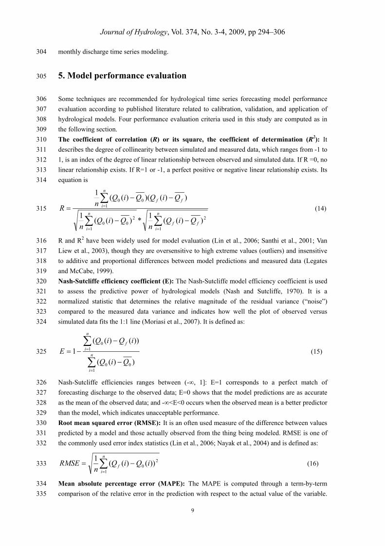
The coefficient of correlation (R) or its square, the coefficient of determination (R2): It 310

describes the degree of collinearity between simulated and measured data, which ranges from -1 to 311

1, is an index of the degree of linear relationship between observed and simulated data. If R =0, no 312

linear relationship exists. If R=1 or -1, a perfect positive or negative linear relationship exists. Its 313

equation is 314

n

iff

n

i

n

iff

QiQn

QiQn

QiQQiQn

R

1

2

1

200

100

))((1

*))((1

))()()((1

(14) 315

R and R2 have been widely used for model evaluation (Lin et al., 2006; Santhi et al., 2001; Van 316

Liew et al., 2003), though they are oversensitive to high extreme values (outliers) and insensitive 317

to additive and proportional differences between model predictions and measured data (Legates 318

and McCabe, 1999). 319

Nash-Sutcliffe efficiency coefficient (E): The Nash-Sutcliffe model efficiency coefficient is used 320

to assess the predictive power of hydrological models (Nash and Sutcliffe, 1970). It is a 321

normalized statistic that determines the relative magnitude of the residual variance (“noise”) 322

compared to the measured data variance and indicates how well the plot of observed versus 323

simulated data fits the 1:1 line (Moriasi et al., 2007). It is defined as: 324

n

i

n

if

QiQ

iQiQE

100

10

))((

))()((1 (15) 325

Nash-Sutcliffe efficiencies ranges between (-∞, 1]: E=1 corresponds to a perfect match of 326

forecasting discharge to the observed data; E=0 shows that the model predictions are as accurate 327

as the mean of the observed data; and -∞<E<0 occurs when the observed mean is a better predictor 328

than the model, which indicates unacceptable performance. 329

Root mean squared error (RMSE): It is an often used measure of the difference between values 330

predicted by a model and those actually observed from the thing being modeled. RMSE is one of 331

the commonly used error index statistics (Lin et al., 2006; Nayak et al., 2004) and is defined as: 332

n

if iQiQ

nRMSE

1

20 ))()((

1 (16) 333

Mean absolute percentage error (MAPE): The MAPE is computed through a term-by-term 334

comparison of the relative error in the prediction with respect to the actual value of the variable. 335


10

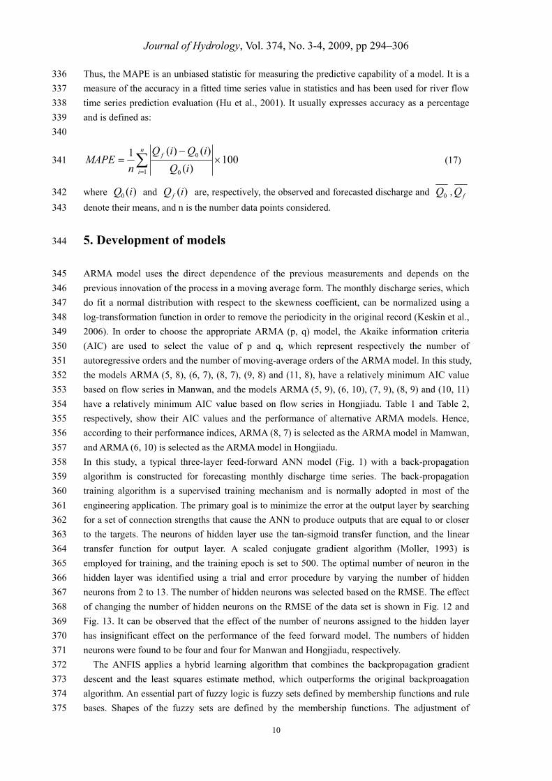
Thus, the MAPE is an unbiased statistic for measuring the predictive capability of a model. It is a 336

measure of the accuracy in a fitted time series value in statistics and has been used for river flow 337

time series prediction evaluation (Hu et al., 2001). It usually expresses accuracy as a percentage 338

and is defined as: 339

340

100)(

)()(1

1 0

0

n

i

f

iQ

iQiQ

nMAPE (17) 341

where )(0 iQ and )(iQf are, respectively, the observed and forecasted discharge and 0Q , fQ 342

denote their means, and n is the number data points considered. 343

5. Development of models 344

ARMA model uses the direct dependence of the previous measurements and depends on the 345

previous innovation of the process in a moving average form. The monthly discharge series, which 346

do fit a normal distribution with respect to the skewness coefficient, can be normalized using a 347

log-transformation function in order to remove the periodicity in the original record (Keskin et al., 348

2006). In order to choose the appropriate ARMA (p, q) model, the Akaike information criteria 349

(AIC) are used to select the value of p and q, which represent respectively the number of 350

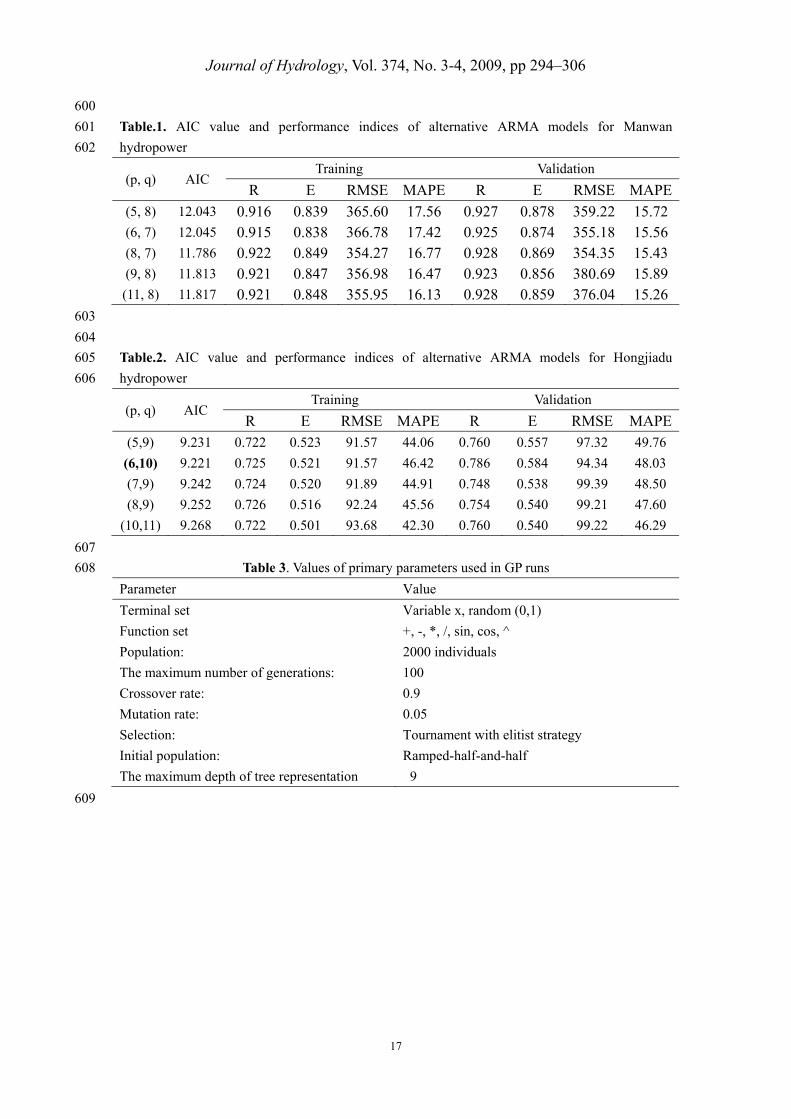
autoregressive orders and the number of moving-average orders of the ARMA model. In this study, 351

the models ARMA (5, 8), (6, 7), (8, 7), (9, 8) and (11, 8), have a relatively minimum AIC value 352

based on flow series in Manwan, and the models ARMA (5, 9), (6, 10), (7, 9), (8, 9) and (10, 11) 353

have a relatively minimum AIC value based on flow series in Hongjiadu. Table 1 and Table 2, 354

respectively, show their AIC values and the performance of alternative ARMA models. Hence, 355

according to their performance indices, ARMA (8, 7) is selected as the ARMA model in Mamwan, 356

and ARMA (6, 10) is selected as the ARMA model in Hongjiadu. 357

In this study, a typical three-layer feed-forward ANN model (Fig. 1) with a back-propagation 358

algorithm is constructed for forecasting monthly discharge time series. The back-propagation 359

training algorithm is a supervised training mechanism and is normally adopted in most of the 360

engineering application. The primary goal is to minimize the error at the output layer by searching 361

for a set of connection strengths that cause the ANN to produce outputs that are equal to or closer 362

to the targets. The neurons of hidden layer use the tan-sigmoid transfer function, and the linear 363

transfer function for output layer. A scaled conjugate gradient algorithm (Moller, 1993) is 364

employed for training, and the training epoch is set to 500. The optimal number of neuron in the 365

hidden layer was identified using a trial and error procedure by varying the number of hidden 366

neurons from 2 to 13. The number of hidden neurons was selected based on the RMSE. The effect 367

of changing the number of hidden neurons on the RMSE of the data set is shown in Fig. 12 and 368

Fig. 13. It can be observed that the effect of the number of neurons assigned to the hidden layer 369

has insignificant effect on the performance of the feed forward model. The numbers of hidden 370

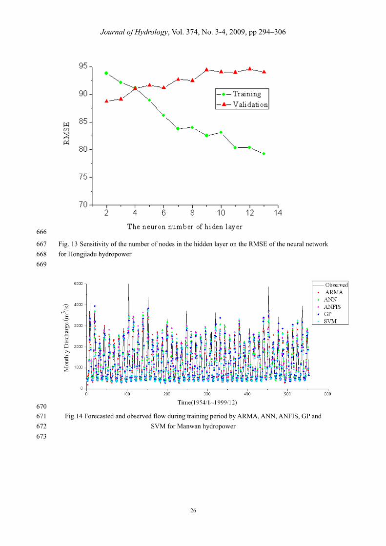
neurons were found to be four and four for Manwan and Hongjiadu, respectively. 371

The ANFIS applies a hybrid learning algorithm that combines the backpropagation gradient 372

descent and the least squares estimate method, which outperforms the original backproagation 373

algorithm. An essential part of fuzzy logic is fuzzy sets defined by membership functions and rule 374

bases. Shapes of the fuzzy sets are defined by the membership functions. The adjustment of 375


11

adequate membership function parameters is facilitated by a gradient vector. After determining a 376

gradient vector, the parameters are adjusted and the performance function is minimised via 377

least-squares estimation. For the proposed Sugeno-type model, the overall output is expressed as 378

linear combinations of the resulting parameters. The output f in Fig. 3 can be rewritten as: 379

2222221111112211 )()()()()()( rwqywpxwrwqywpxwfwfwf (18) 380

The resulting parameters (p1, q1, r1, p2, q2, r2) are computed by the least-squares method. 381

Consequently, the optimal parameters of the ANFIS model can be estimated using the hybrid 382

learning algorithm. For more detail, please refer to Jang and Sun (Jang et al., 1997). 383

GP has the ability to generate the best computer program to describe the relationship between 384

the input and output. In this study, in order to find the optimal monthly flow series forecasting 385

model, the selection of the appropriate parameters of GP evolution is necessary. Although the 386

fine-tuning of algorithm was not the main concern of this paper, we investigated various 387

initialization and run approaches and the adopted GP parameters are presented in Table 3. This 388

setup furnished stable and effective runs throughout experiments. The evolutionary procedures are 389

similar to GAs including defining the fitness function, genetic operators such as crossover, 390

mutation and reproduction and the termination criterion, etc. In GP, the crossover operator is used 391

to swap the subtree from the parents to reproduce the children using mating selection policy rather 392

than exchanging bit strings as in GAs. 393

A kernel function has to be selected from the qualified functions in using SVM. Dibike et al. 394

(2001) applied different kernels in SVR to rainfall- runoff modeling and demonstrated that the 395

radial basis function (RBF) outperforms other kernel functions. Also, many works on the use of 396

SVR in hydrological modeling and forecasting have demonstrated the favorable performance of 397

the RBF (Khan and Coulibaly, 2006; Lin et al., 2006; Liong and Sivapragasam, 2002; Yu et al., 398

2006). Therefore, the RBF is used as the kernel function for prediction of discharge in this study. 399

There are three parameters in using RBF kernels: C, ε and σ. the accuracy of a SVM model is 400

largely dependent on the selection of the model parameters. However, structured methods for 401

selecting parameters are lacking. Consequently, some kind of model parameter calibration should 402

be made. Recently, there are several methods developed to identify the parameters, such as the 403

simulated annealing algorithms (Pai and Hong, 2005), GA (Pai, 2006) and the shuffled complex 404

evolution algorithm (SCE-UA) (Lin et al., 2006; Yu et al., 2004). The SCE-UA method belongs to 405

the family of evolution algorithm and was presented by Duan et al. (1993). In this study, the 406

SCE-UA is employed as the method of optimizing parameters of SVM and a more comprehensive 407

presentation can be found by Lin et al. (2006). To reach at a suitable choice of these parameters, 408

the RMSE was used to optimize the parameters. Optimal parameters (C, ε, σ) = (19.9373, 409

8.7775e-004, 1.2408) and (C, ε, σ) = (0.5045, 5.0814e-004, 0.6623) were obtained for Manwan 410

and Hongjiadu, respectively. 411

6. Results and discussion 412

The Manwan Hydropower, has been studied by Cheng et al. (2005) using ANFIS with 413

discharges of monthly river flow discharges during 1953-2003, and by Lin et al. (2006) using 414

SVM with discharges of monthly river flow discharges during 1974-2003. In their study, the R and 415

RMSE were employed for evaluation model performance. In this paper, in order to identify more 416


12

suitable models for forecasting future monthly inflows to hydropower reservoirs, the monthly 417

discharge time series data of two study sites in different rivers are applied. For the same basis of 418

comparison, the same training and verification sets, respectively, are used for all the above models 419

developed, whilst the four quantitative standard statistical performance evaluation measures are 420

employed to evaluate the performances of various models developed. Tables 4 and 5 present the 421

results of Manwan and Hongjiadu study sites respectively, in terms of various performance 422

statistics 423

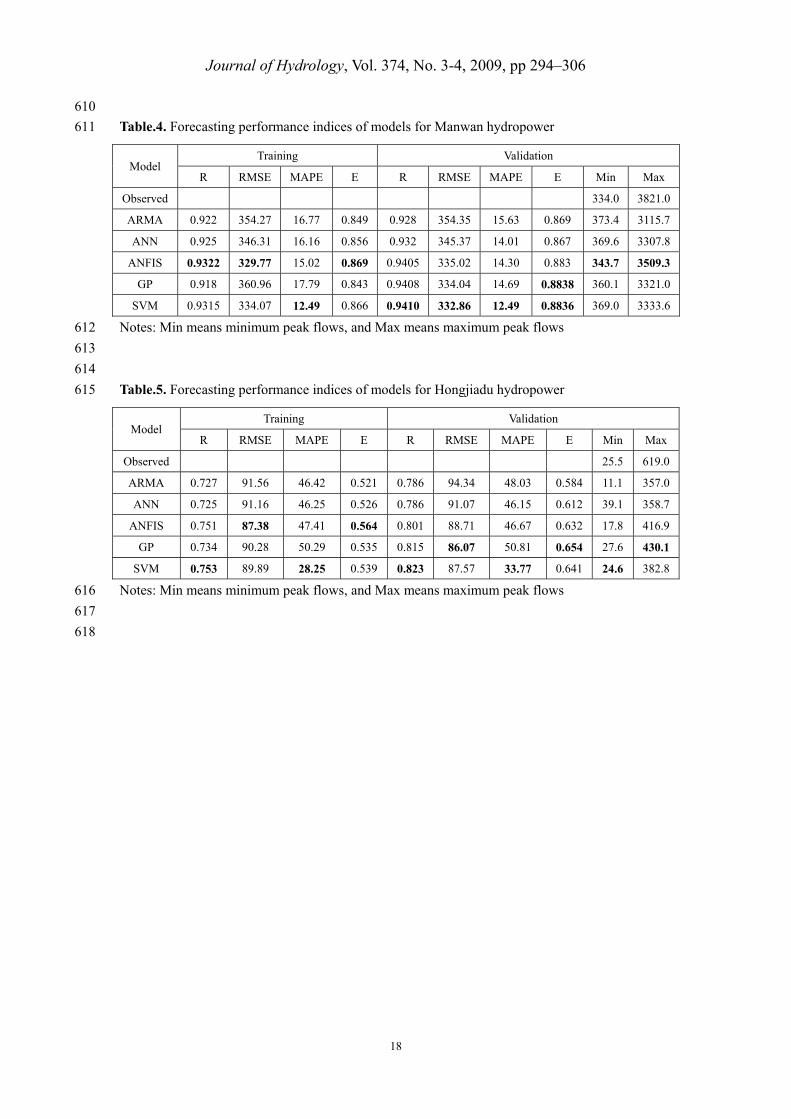
It can be observed from Tables 4 and 5 that various AI methods have good performance during 424

both training and validation, and they outperform ARMA in terms of all the standard statistical 425

measures. For Manwan hydropower, in the training phase, the ANFIS model obtained the best R, 426

RMSE, and E statistics of 0.932, 329.77, and 0.869, respectively; while the SVM model obtained 427

the best MAPE statistics of 12.49. Analyzing the results during testing, it can be observed that the 428

SVM model outperforms all other models. Similarly, for Hongjiadu hydropower, in the training 429

phase, the ANFIS model obtained the best RMSE and E statistics of 887.38 and 0.564, 430

respectively; while the SVM model obtained the best R and MAPE statistics of 0.753 and 28.25, 431

respectively. Analyzing the results during testing, the SVM model obtained the best R and MAPE 432

statistics of 0.823 and 33.77, respectively; while the GP model obtained the best RMSE, and E 433

statistics of 86.07 and 0.654, respectively. RMSE evaluates the residual between observed and 434

forecasted flow, and MAPE measures the mean absolute percentage error of the forecast. R 435

evaluates the linear correlation between the observed and computed flow, while E evaluates the 436

capability of the model in predicting flow values away from the mean. According to the figures in 437

Tables 4 and 5, we can conclude that the best performance of all AI methods developed in this 438

paper is different in terms of the different statistical measures. 439

In addition, in the validation phase as seen in Tables 4 and 5, the values with the ANFIS, GP and 440

SVM model prediction were able to produce a good, near forecast, as compared to those with 441

ARMA and ANN model, whilst it can be concluded that the ANFIS model obtained the best 442

minimum absolute error between the observed and modeled maximum and minimum peak flows 443

in Manwan Hydropower, and the GP and SVM model obtained the best minimum absolute error 444

between the observed and modeled maximum and minimum peak flows, respectively, in 445

Hongjiadu Hydropower. In the validation phase, the SVM model improved the ARMA forecast of 446

about 6.06% and 20.12% reduction in RMSE and MAPE values, respectively; Improvements of 447

the forecast results regarding the R and E were approximately 1.22% and 1.69%, respectively in 448

Manwan Hydropower. In Hongjiadu Hydropower, the GP model obtained the best value of RMSE 449

during the validation phase decreases by 8.77% and the best value of E increases by 11.99% 450

comparing with ARMA; while, the SVM model obtained the best value of R during the validation 451

phase increases by 4.71% and the best value of MAPE decreases by 29.69% comparing with 452

ARMA. Thus the results of this analysis indicate that the ANFIS or SVM is able to obtain the best 453

result in terms of different evaluation measures during the training phase, and the GP or SVM is 454

able to obtain the best result in terms of different evaluation measures during the validation phase. 455

Furthermore, as can be seen from Tables 4 and 5 that the virtues or defect degree of forecasting 456

accuracy is different in terms of different evaluation measures during the training phase and the 457

validation phase. SVM model is able to obtain the better forecasting accuracy in terms of different 458

evaluation measures during the validation phase not only during the training phase but also during 459

the validation phase. The forecasting results of ANFIS model during the validation phase are 460


13

inferior to the results during the training phase. GP is in the middle or lower level in training 461

phases, but the GP model is able to obtain the better forecasting result in validation phases, and 462

especially the GP model is able to obtain the maximum peak flows among all models developed in 463

Hongjiadu Hydropower. The performances of all prediction models developed in this paper during 464

the training and validation periods in the two study sites are shown in Fig. 14 to. 17. 465

7. Conclusions 466

An attempt was made in this study to investigate the performance of several AI methods for 467

forecasting monthly discharge time series. The forecasting methods investigated include the ANNs 468

ANFIS techniques, GP models and SVM method. The conventional ARMA is also employed as a 469

benchmarking yardstick for comparison purposes. The monthly discharge data from actual field 470

observed data in the Manwan Hydropower and Hongjiadu Hydropower were employed to develop 471

various models investigated in this study. The methods utilize the statistical properties of the data 472

series with certain amount of lagged input variables. Four standard statistical performance 473

evaluation measures are adopted to evaluate the performances of various models developed. 474

The results obtained in this study indicate that the AI methods are powerful tools to model the 475

discharge time series and can give good prediction performance than traditional time series 476

approaches. The results indicate that the best performance can be obtained by ANFIS, GP and 477

SVM, in terms of different evaluation criteria during the training and validation phases. SVM 478

model is able to obtain the better forecasting accuracy in terms of different evaluation measures 479

during the validation phase during both the training phase and the validation phase. The 480

forecasting results of ANFIS model during the validation phase are inferior to the results during 481

the training phase. GP is in the middle or lower level in training phases, but the GP model is able 482

to obtain the better forecasting result in validation phases. The ANFIS and GP model obtain the 483

maximum peak flows among all models developed in different studies sites, respectively. 484

Therefore, the results of the study are highly encouraging and suggest that ANFIS, GP and SVM 485

approaches are promising in modeling monthly discharge time series, and this may provide 486

valuable reference for researchers and engineers who apply AI methods for modeling long-term 487

hydrological time series forecasting. It is hoped that future research efforts will focus in these 488

directions, i.e. more efficient approach for training multi-layer perceptrons of ANN model, the 489

increased learning ability of the ANFIS model, the fine-tuning of algorithm for selecting more 490

appropriate parameters of GP evolution, saving computing time or more efficient optimization 491

algorithms in searching optimal parameters of SVM model etc to improve the accuracy of the 492

forecast models in terms of different evaluation measures for better planning, design, operation, 493

and management of various engineering systems. 494

Acknowledgements 495

This research was supported by the Central Research Grant of Hong Kong Polytechnic University 496

(G-U265), the National Natural Science Foundation of China (No.50679011), Doctor Foundation 497

of higher education institutions of China (No.20050141008). 498


14

Reference 499

ASCE Task Committee., 2000a. Artificial neural networks in hydrology-I: Preliminary concepts. 500

Journal of Hydrologic Engineering, ASCE 5(2): 115-123. 501

ASCE Task Committee., 2000b. Artificial neural networks in hydrology-II: Hydrological 502

applications. Journal of Hydrologic Engineering, ASCE5(2): 124-137. 503

Asefa, T., Kemblowski, M., McKee, M. and Khalil, A., 2006. Multi-time scale stream flow 504

predictions: The support vector machines approach. Journal of Hydrology, 318(1-4): 7-16. 505

Bazartseren, B., Hildebrandt, G. and Holz, K.P., 2003. Short-term water level prediction using 506

neural networks and neuro-fuzzy approach. Neurocomputing, 55(3-4): 439-450. 507

Borrelli, A., De Falco, I., Della Cioppa, A., Nicodemi, M. and Trautteur, G., 2006. Performance of 508

genetic programming to extract the trend in noisy data series. Physica a-Statistical 509

Mechanics and Its Applications, 370(1): 104-108. 510

Box, G.E.P. and Jenkins, G.M., 1970. Times series Analysis Forecasting and Control. Holden-Day, 511

San Francisco. 512

Campolo, M., Soldati, A. and Andreussi, P., 2003. Artificial neural network approach to flood 513

forecasting in the River Arno. Hydrological Sciences Journal, 48(3): 381-398. 514

Chang, L.C. and Chang, F.J., 2001. Intelligent control for modelling of real-time reservoir 515

operation. Hydrological Processes, 15(9): 1621-1634. 516

Chau, K.W., 2006. Particle swarm optimization training algorithm for ANNs in stage prediction of 517

Shing Mun River. Journal of Hydrology, 329(3-4): 363-367. 518

Chau, K.W. and Cheng, C.T., 2002. Real-time prediction of water stage with artificial neural 519

network approach. Lecture Notes in Artificial Intelligence, 2557: 715. 520

Chen, H.L. and Rao, A.R., 2002. Testing hydrologic time series for stationarity. Journal of 521

Hydrologic Engineering, 7(2): 129-136. 522

Cheng, C.T., Lin, J.Y., Sun, Y.G. and Chau, K.W., 2005. Long-term prediction of discharges in 523

Manwan hydropower using adaptive-network-based fuzzy inference systems models, 524

Advances in Natural Computation, Pt 3, Proceedings. Lecture Notes in Computer Science. 525

Springer-Verlag Berlin, Berlin, pp. 1152-1161. 526

Dibike, Y.B., Velickov, S., Solomatine, D. and Abbott, M.B., 2001. Model induction with support 527

vector machines: Introduction and applications. Journal of Computing in Civil 528

Engineering, 15(3): 208-216. 529

Dixon, B., 2005. Applicability of neuro-fuzzy techniques in predicting ground-water vulnerability: 530

a GIS-based sensitivity analysis. Journal of Hydrology, 309(1-4): 17-38. 531

Duan, Q.Y., Gupta, V.K. and Sorooshian, S., 1993. Shuffled complex evolution approach for 532

effective and efficient minimization. Journal of Optimization Theory and Applications, 533

76(3): 501-521. 534

Haykin, S., 1999. Neural networks: a comprehensive foundation. 2nd ed. Upper Saddle River, 535

New Jersey. 536

Hu, T.S., Lam, K.C. and Ng, S.T., 2001. River flow time series prediction with a range-dependent 537

neural network. Hydrological Sciences Journal, 46(5): 729-745. 538

Jang, J.-S.R., 1993. ANFIS: Adaptive-Network-based Fuzzy Inference Systems. IEEE 539

Transactions on Systems, Man, and Cybernetics, 23(3): 665-685. 540

Jang, J.-S.R., Sun, C.-T. and Mizutani, E., 1997. Neuro-Fuzzy and Soft Computing: A 541


15

Computational Approach to Learning and Machine Intelligence. Prentice-Hall, Upper 542

Saddle River, NJ. 543

Johari, A., Habibagahi, G. and Ghahramani, A., 2006. Prediction of soil-water characteristic curve 544

using genetic programming. Journal of Geotechnical and Geoenvironmental Engineering, 545

132(5): 661-665. 546

Keskin, M.E., Taylan, D. and Terzi, O., 2006. Adaptive neural-based fuzzy inference system 547

(ANFIS) approach for modelling hydrological time series. Hydrological Sciences Journal, 548

51(4): 588-598. 549

Khan, M.S. and Coulibaly, P., 2006. Application of support vector machine in lake water level 550

prediction. Journal of Hydrologic Engineering, 11(3): 199-205. 551

Koza, J., 1992. Genetic Programming: On the Programming of Computers by Natural Selection. 552

MIT Press, Cambridge, MA. 553

Legates, D.R. and McCabe, G.J., 1999. Evaluating the use of "goodness-of-fit" measures in 554

hydrologic and hydroclimatic model validation. Water Resources Research, 35(1): 555

233-241. 556

Lin, J.Y., Cheng, C.T. and Chau, K.W., 2006. Using support vector machines for long-term 557

discharge prediction. Hydrological Sciences Journal, 51(4): 599-612. 558

Liong, S.Y. et al., 2002. Genetic Programming: A new paradigm in rainfall runoff modeling. 559

Journal of the American Water Resources Association, 38(3): 705-718. 560

Liong, S.Y. and Sivapragasam, C., 2002. Flood stage forecasting with support vector machines. 561

Journal of the American Water Resources Association, 38(1): 173-186. 562

Moller, M.F., 1993. A scaled conjugate gradient algorithm for fast supervised learning. Neural 563

Networks, 6(4): 525-533. 564

Moriasi, D.N. et al., 2007. Model evaluation guidelines for systematic quantification of accuracy 565

in watershed simulations. Transactions of the ASABE, 50(3): 885-900. 566

Muttil, N. and Chau, K.W., 2006. Neural network and genetic programming for modelling coastal 567

algal blooms. International Journal of Environment and Pollution, 28(3-4): 223-238. 568

Nash, J.E. and Sutcliffe, J.V., 1970. River flow forecasting through conceptual models part I — A 569

discussion of principles. Journal of Hydrology, 10(3): 282-290. 570

Nayak, P.C., Sudheer, K.P., Rangan, D.M. and Ramasastri, K.S., 2004. A neuro-fuzzy computing 571

technique for modeling hydrological time series. Journal of Hydrology, 291(1-2): 52-66. 572

Pai, P.-F., 2006. System reliability forecasting by support vector machines with genetic algorithms. 573

Mathematical and Computer Modelling, 43(3-4): 262-274. 574

Pai, P.-F. and Hong, W.-C., 2005. Support vector machines with simulated annealing algorithms in 575

electricity load forecasting. Energy Conversion and Management, 46(17): 2669-2688. 576

Salas, J.D., 1993. Analysis and modeling of hydrologic time series. In: Maidment, D.R., Editor, 577

1993. The McGraw Hill Handbook of Hydrology, pp. 19.5–19.9. 578

Santhi, C. et al., 2001. Validation of tbe swat model on a large river basin with point and nonpoint 579

sources. Journal of the American Water Resources Association, 37(5): 1169-1188. 580

Sivapragasam, C., Vincent, P. and Vasudevan, G., 2007. Genetic programming model for forecast 581

of short and noisy data. Hydrological Processes, 21(2): 266-272. 582

Srikanthan, R. and McMahon, T.A., 2001. Stochastic generation of annual, monthly and daily 583

climate data: A review. Hydrology and Earth System Sciences, 5(4): 653-670. 584

Sudheer, K.P., Gosain, A.K. and Ramasastri, K.S., 2002. A data-driven algorithm for constructing 585


16

artificial neural network rainfall-runoff models. Hydrological Processes, 16(6): 586

1325-1330. 587

Van Liew, M.W., Arnold, J.G. and Garbrecht, J.D., 2003. Hydrologic simulation on agricultural 588

watersheds: Choosing between two models. Transactions of the Asae, 46(6): 1539-1551. 589

Vapnik, V., 1995. The Nature of Statistical Learning Theory. Springer, New York. 590

Vapnik, V., 1998. Statistical learning theory. Wiley, New York. 591

Whigam, P.A. and Crapper, P.F., 2001. Modelling Rainfall-Runoff Relationships using Genetic 592

Programming. Mathematical and Computer Modelling 33: 707-721. 593

Yu, P.S., Chen, S.T. and Chang, I.F., 2006. Support vector regression for real-time flood stage 594

forecasting. Journal of Hydrology, 328(3-4): 704-716. 595

Yu, X.Y., Liong, S.Y. and Babovic, V., 2004. EC-SVM approach for real-time hydrologic 596

forecasting. Journal of Hydroinformatics, 6(3): 209-223. 597

598

599


17

600

Table.1. AIC value and performance indices of alternative ARMA models for Manwan 601

hydropower 602

(p, q) AIC Training Validation

R E RMSE MAPE R E RMSE MAPE(5, 8) 12.043 0.916 0.839 365.60 17.56 0.927 0.878 359.22 15.72 (6, 7) 12.045 0.915 0.838 366.78 17.42 0.925 0.874 355.18 15.56 (8, 7) 11.786 0.922 0.849 354.27 16.77 0.928 0.869 354.35 15.43 (9, 8) 11.813 0.921 0.847 356.98 16.47 0.923 0.856 380.69 15.89 (11, 8) 11.817 0.921 0.848 355.95 16.13 0.928 0.859 376.04 15.26 603

604

Table.2. AIC value and performance indices of alternative ARMA models for Hongjiadu 605

hydropower 606

(p, q) AIC Training Validation

R E RMSE MAPE R E RMSE MAPE(5,9) 9.231 0.722 0.523 91.57 44.06 0.760 0.557 97.32 49.76

(6,10) 9.221 0.725 0.521 91.57 46.42 0.786 0.584 94.34 48.03

(7,9) 9.242 0.724 0.520 91.89 44.91 0.748 0.538 99.39 48.50

(8,9) 9.252 0.726 0.516 92.24 45.56 0.754 0.540 99.21 47.60

(10,11) 9.268 0.722 0.501 93.68 42.30 0.760 0.540 99.22 46.29

607

Table 3. Values of primary parameters used in GP runs 608

Parameter Value

Terminal set Variable x, random (0,1)

Function set +, -, *, /, sin, cos, ^

Population: 2000 individuals

The maximum number of generations: 100

Crossover rate: 0.9

Mutation rate: 0.05

Selection: Tournament with elitist strategy

Initial population: Ramped-half-and-half

The maximum depth of tree representation 9

609


18

610

Table.4. Forecasting performance indices of models for Manwan hydropower 611

Model Training Validation

R RMSE MAPE E R RMSE MAPE E Min Max

Observed 334.0 3821.0

ARMA 0.922 354.27 16.77 0.849 0.928 354.35 15.63 0.869 373.4 3115.7

ANN 0.925 346.31 16.16 0.856 0.932 345.37 14.01 0.867 369.6 3307.8

ANFIS 0.9322 329.77 15.02 0.869 0.9405 335.02 14.30 0.883 343.7 3509.3

GP 0.918 360.96 17.79 0.843 0.9408 334.04 14.69 0.8838 360.1 3321.0

SVM 0.9315 334.07 12.49 0.866 0.9410 332.86 12.49 0.8836 369.0 3333.6

Notes: Min means minimum peak flows, and Max means maximum peak flows 612

613

614

Table.5. Forecasting performance indices of models for Hongjiadu hydropower 615

Model Training Validation

R RMSE MAPE E R RMSE MAPE E Min Max

Observed 25.5 619.0

ARMA 0.727 91.56 46.42 0.521 0.786 94.34 48.03 0.584 11.1 357.0

ANN 0.725 91.16 46.25 0.526 0.786 91.07 46.15 0.612 39.1 358.7

ANFIS 0.751 87.38 47.41 0.564 0.801 88.71 46.67 0.632 17.8 416.9

GP 0.734 90.28 50.29 0.535 0.815 86.07 50.81 0.654 27.6 430.1

SVM 0.753 89.89 28.25 0.539 0.823 87.57 33.77 0.641 24.6 382.8

Notes: Min means minimum peak flows, and Max means maximum peak flows 616

617

618


19

619

List of all figures 620

621

622 Fig.1. Architecture of three layers feed-forward back-propagation ANN 623

624

625

626

Fig.2. Two inputs first-order Sugeno fuzzy model with two rules 627


20

628

Fig.3. Architecture of ANFIS 629

630

631

632

Fig. 4. GP parse tree representing function abacb 2)4( 2 633

634


21

635

Fig. 5. The basis of the support vector machines. 636

637

638

Fig.6. The soft margin loss setting for a linear SVM and ε-insensitive loss function 639

640

641


22

642

Fig. 7. Monthly discharge at Manwan Reservoir 643

644


23

645

646

Fig. 8 Location of study sites 647

648

649


24

650

Fig. 9 Monthly discharge at Hongjiadu Reservoir 651

652

653 Fig.10. (a) the autocorrelation function of flow series. (b)The partial autocorrelation function of 654

flow series in Manwan 655

656

657


25

658

Fig.11 (a) The autocorrelation function of flow series. (b)The partial autocorrelation function of 659

flow series in Hongjiadu. 660

661

662 Fig. 12 Sensitivity of the number of nodes in the hidden layer on the RMSE of the neural network 663

for Manwan hydropower 664

665


26

666

Fig. 13 Sensitivity of the number of nodes in the hidden layer on the RMSE of the neural network 667

for Hongjiadu hydropower 668

669

670

Fig.14 Forecasted and observed flow during training period by ARMA, ANN, ANFIS, GP and 671

SVM for Manwan hydropower 672

673


27

674

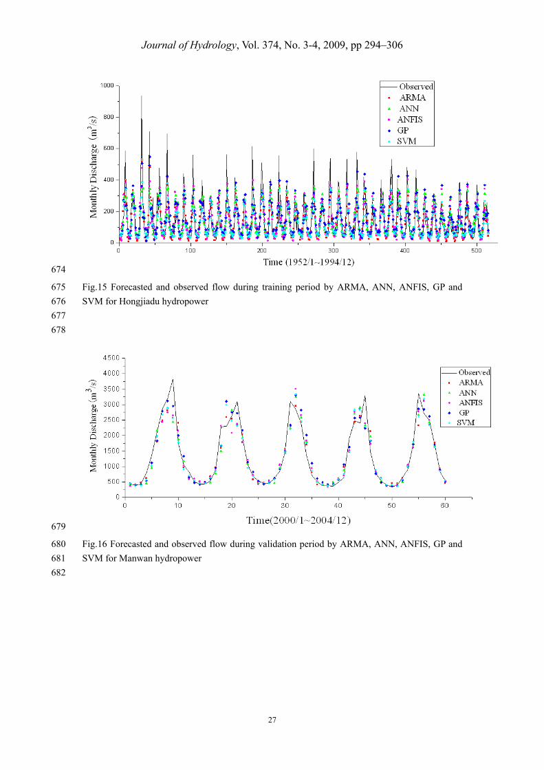
Fig.15 Forecasted and observed flow during training period by ARMA, ANN, ANFIS, GP and 675

SVM for Hongjiadu hydropower 676

677

678

679

Fig.16 Forecasted and observed flow during validation period by ARMA, ANN, ANFIS, GP and 680

SVM for Manwan hydropower 681

682


28

683

Fig.17 Forecasted and observed flow during validation period by ARMA, ANN, ANFIS, GP and 684

SVM for Hongjiadu hydropower 685

Documents

A comparison of performance of several artificial intelligence