Embed Size (px)
Citation preview

A COMPARATIVE STUDY OF CAPITAL BUDGETING AND CAPITAL RATIONING MODELS AS AN ANALYSIS FOR CAPITAL INVESTMENT DECISIONS
A literature study
done by: ,Churiah Agustini Santoso
\9f199 \2.-1 Pls:rp
UNIVERSITAS KATOLIK PARAHYANGAN FAKULTAS ILMU SOSIAL DAN ILMU POLITIK
BAN DUNG 1984
9-1 <;;. . [)'6
No. Klass ?~.~.:.(,(:') .. 9.:t.-: ... ;:;. No. Induk.l?:\!~c~ Tgi .~~.:~.;~. t-Iadioh/lleli ........................... .

TAiLE Of CONTENTS
page
ABSTRACT i
TABLE Of CONTENTS ii
CHAPTER 1
CHAPTER 2. 2.1 2.2 2.3 2 4 2.5 2.6
CHAPTER 3. 3.1 3.2 3 3 3.4
3.5 36
CHAPTER 4. 4.1 4.2
. 4.3
CHAPTER 5 5.1 5.2 5.3 5 4
CHAPTER 6.
6.1 6.2 6.3 64 6.5
CHAPTER 7
INTRODUCTION ..... 1
CAPITAL BUDGETING UNDER CERTAINTy •........••.•••... 4 Net Present Value ................................ 4 Payback ..•••..•••.....•••...•••••...•.•.••.•.•.•.• 5 Average Return on Book Value ....................... 6 Internal Rate of Return ..•.......•.......•..••..•• 8 Profitability Index ....................... 10 Application on The Investment Analys:'.s •.....••.. Program .................................... 11
CAPITAL RATIONING UNDER CERTAINTy ....•.••.••...... 16 Definition ...................................... 16 Structure ...................................... 17 Profitability Index. . ........................ 17 Ma themetica 1 Programming Linea r ....•........•... Programming. . • . . • . . . . . . • . . . • . . . . . • . . . . • . . . . . .. .. 19 Integer Programming ............................. 29 Goal Programm:'.ng •.......•.................• 34
CAPITAL BUDGETING UNDER UNCERTAINTy ..•......•..... 40 Sen~i~ivi~y Analysis/ Break-even Analysis ........ 40 DeCl.S10n frees .•.................................. 42 Simulation ........................................... 5
CAPITAL RATIONING UNDER UNCERTAINTy ..........•.... 52 Stochastic Li.near Programmi.ng ....................• 52 Chance-contra:'.ned Programming ..................... 53 Quadratic Programming ............................. 53 An Example by Salazar and Sen .................... 54
DESCRIPTION OF THE SENSITIVITY ANALySIS; ......... . PROGRAM .................... ; •......•....•..•... 59 Assumptions .....•.....•...........•............... 59 In pu t D a t a ..•.........•......•.......•.•.....•.... 59 Flowchart of The Program ....................•..... 60 Output Data ....•.............•.....•..•........... 63 Example ...............•.........................• 63
SUHt·1ARy ........................................... 67
i(i'""""RFNC' . --.c.. bS ............•...........•........................... 68
Ai)P[\DIX . . . ...........................•.............•............ 70
. . 1 1

ABSTRACT
lhe process of planning and evaluating
is called capital budget~ng. Capital
proposals t6r ~nvestments
budgeting dec~sions are
important because large 880unt ot money are committee tor long
periods of time and because these type ot decis~on are often
difficult or impossible to reverse once the funds have been
committee.
Th~s stUdy surveys difterent models dnd techniques that are used
to solve several types of ~~~i_a. bld~eting problems These types
are of simple capital budgeting and capital rationing; under
conditions ot certainty and uncertainty
·lhe analysis helps on the difficult and critical deCisions
management has to make
_ 1

The field
comprehensive and
in assisting most
goals.
or ~s~~_~_ ~nvesLment analysis is both
c~s~~=~~~=g. It clearly plays a vital role
tus~~ess ~~~ms to achieve their various
Capital budgec~=~ ~s :~e
management which esta~~~shes
investing
investment
resources
projects
long
co~conly
t~e
decision area in financial
goals and criteria for
term projects. Capital
include land, buildings,
like. These assets are facilities, equipmeD~, and
extremely important ~o :~e
all of the firm's ?r0f~t
fir~ because, in general,
are derived from the use nearly
of its capital investments; ~hese assets represent very large
commitments of resources; and c~e funds ~ill usually remain
invested over a long ?eriod of time. The future development
investment of the firm hinges on the selection of capital
projects, and the decision to abandon previously
undertakin~s which turn out to be less attractive
firm than was originally thought~
accepted
to the
The benefits of capital projects are received Over some future period, and the time element lies at the core of
capital budgeting. The firm must time the start of a project
to take advantage of short-ter~ business conditions
(construction costs for example vary ~ith the stage of
business cycle) and financing of the project to capitalize
on trends in the money markets (such as the pattern of short
and long term interest ra(2), In addition, the longevity of
capital assets and the ~3rge outlays required for their
acquisition suggest tha: :je estimates of income and cost
aSSOCiated with the pro:e:: to be documented for the time

are
:.~ons
--::..ence
2
received or out Moreover, investment
are al~ays bas~: JPon incomplete information using
of fut~re reve=':~s and costs. It is known from the
that such fC~~:25~s will always err on one side
~~e other, and the de;=~e of error may correlate "(but not
:'J.J;':;1"S) with the durat:::: of the projects. Short-term
(1 year or ::'''5S) generally display greater
than long-ter::! =stimates (S years or more). The
:; dimly seen enta:":"~ risk, and any appraisal of a
(_~:. ~ "'_21 project 1 therefo::;;;:. must necessarily comprehend some
,,"';'" ",ocsment of the risk =.c::ompanying the project. Finally,
.... ,~:;.tment , " decisions mus::. be matched aga~nst some future
to ascertain t~e accur~cy of the forecast and the
·/j;:.;",,:·.L~ty of evaluating c::~teria. In summary, the components
'if '.cpital budgeting
cost.s of
a=E~ysis involve n forecast of the
and project, discounting the funds
j fl 'f!-; .~ ted in the project 8,\:. an appropriate
project and
rate, assessing
following up to 1 11 {- associated wit:: the
Ill" I~:~i.ne if the project pe~:orm cs expected.
The application of capital budgeting are many
'I ;; r : .~ rj • In theory, a :arge n urn be r or problems
and
lend
1 J I 1". /f, .'~ e 1 v e s to analysis by 'lar~ous methods. Analysis absorbs
! i I:, (:
I!! 1/ :~ !.
,,,
and ::noney, especiall J :he more
ranking and risk management. The
sophisticated tec~niques
cost of these approaches
be justified by the ?erceived benefits~ Theory adapts
costly circumstances. Conceptually appealing but
! P' :Jniques of analysis do not merit ac=oss-the-board
:\ !' jI j j r:: a t ion. Accordingly, in establishing a cutoff by .size
(~xpenditure; that is, projects requiring an investment
,,\, ': [ a specified amount ..,il1 be subject to searching.
.; 1 I {j!. 1 n y ; below this amount, less costly criteria of
1'1 l~ptahce will be applied.
This study is an attempt to survey dif£ere~t models
.\ 11.1 t~c.hniques tha~ are used to solve several types or , 'li I 1..j 1 budgetiag problems. In the first place we make a

3
~~~~~~ction between conditions of certainty and
_ -c:: certain t y . Another important distinction
conditions
is bet;..reen
budgeting problems (no capital restriction) and
~~o~tal rationing problems (capital restriction).
Chapter 2 summarizes some techniques to solve the
s~~ital budgeting problem under certainty. Five alternatives
discussed net present value, payback period. average
on book value, internal rate of return and
~r~f~tability index.
These simple techniques cannot be used in situations
where the capital budget is limited. Chapter 3 investigates
30me techniques that can be used to solve the capital
rationing problem under certainty. Simple techniques, like
the ranking based on the profitability index proposed by
Lorie-Savage, can be used when there is a restriction in
()nl'f one
be used:
period. Otherwise mathematical programming should
this can be linear programming, integer programming
or goal programming.
Chapters 4 and 5 handle conditions or uncertainty.
Techniques
budgeting
;J n (] 1 y sis,
problem
break
that can be used to -solve the capital
under uncertainty are: sensitivity
even analysis, decision trees and
~imulation. These techniques are described in chapter 4.
Finally,
uncertainty is
't" .lne capital rationing problem under
discussed in chapter 5~ He~e, a combination
llf mathematical programming and simulation can be used, like
S.llazar and Sen proposed in their paper.
Most of the discussed techniques are illustrated with
t~xamples • For this purpose,programs available on the apple
(.omputers of the department Industrieel 3eleid have been
:lsed. The' existing capital budgeting package did not include
3 sensitivity analysis. That is why a new program was
jt~veloped • This program and some examples are discussed in
: ~1.) pte r 6.

Chapter 2.
CAPITAL 3CDGETI~G UNDER CERTAINTY.
In order to be 301e to perform an economic evaluation
of a project's desiraDil~ty. it is necessary to understand
the decision rule for accepting or rejecting investment
projects. Some methods whic~ guide management in the
acceptance or rejecc~on of proposed investments are
explained in this chapter.
2.l.Net present value.
This measure is a direct application of the present
value concept. Its computation requires the following steps:
first, choose an appropriate rate of interest4 Second,
compute the present value of the substr~ction of the cash
outl~ys from the invescment from the cash proceeds ex"ected
from the inves~ment. This gives the present value or cash flows·. The present value of the cash flows minus
initial investment is the net present value of
investment.
The recommended accept or reject criterion is
the
the
the
to
accept all independent investments whose net present value
is g,reater or equal to zero and reject all invest~ents ~hose
net present value is less than zero.
The formula for calculating PV and NPV can simply be written
as:
P'I ~ C1/0+r) + C2!(l+r;: + ••. + Cn/(l+r)'.'I.
~iPV ~ - CO + PV
4
with :
C1.C2 •••• Cn - Cash flows:of the investment.
r - Interest rate.
CO - The initial investment.
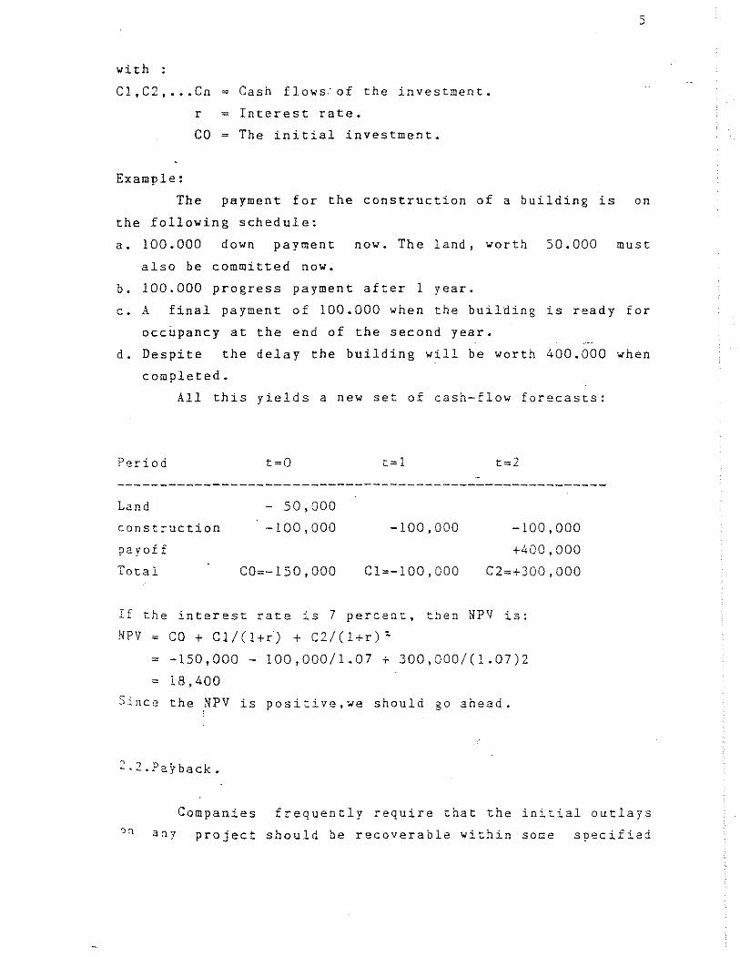
Example:
5
The payment for the construction of a building is on
the following schedule:
a. 100.000 down payment now. The land. worth 50.000 must
also be committed now.
b. 100.000 progress payment after 1 year.
c. A final payment of 100.000 when the building is ready for
occupancy at the end of the second year.
d. Despite the delay the building will be worth 400.000 when
completed.
All this yields a new set of cash-flow forecasts:
Period t==l
Land - 50.000
const:-uction
payoif
Total
-100.000
CO--150.000
-100.000
C1--100,000
-100.000
+400.000
C2-+300,000
If the interest rate is 7 percent, then NPV is:
NPV CO + Cl/Cl+r) + C2/(l+r)'
- -150.000 - 100,000/1.07 + 300,000/(1.07)2
- 18,400
Since the NPV is positive,we should go ahead.
1 1 P . b ... --. 201 ack.
Companies frequently require that the initial olltlays
a:1Y project should be recoverable within some specified

cutoff period.
counting the number
:;eriod
-~"rs it
- - 3 project is
~:'!kes before
forecasted cash flows e~'~~--_ :~e init~21 investment.
Example:
Consider projects A and --
Project
A
B
Cash f::.~.:~llars
========;;:;;=====:;;;;====.=========
CO
-2000
-2000
Cl
+2000
+1000
C3
o +5000
Payback
?eriod,years
1
2
6
found by
cumulated
NPV at
10 :
-182
+3492
The NPV rule tells
project A, we take 1 ye~~
B we take 2 years.
uS to reject A and accept B. With
cO recover our 2000, with project
If the firm use= the pavback rple with a cutoff
period of 1 year, it woc~d accept only project A. If it used
the payback rule with a 2utoff period of 2 or more years it
would accept both A an& 3. The reason for the difference is
that payback gives equal weight to all cash flows before
payback date and no weight at all to subsequent flows.
order to use the payback rule the firm has to decide on
appropriate cutoff date.
2.3.Average retur~ on book value.
the
In an
Some companies jud~= an investment project by looking
at its book rate of retur~. To calculate book rate of return
it is necessary to divide :ie average forecasted profits of
a project after deprec:~::on and taxes, by the average
r~turn on book value of ::e investment. This ratio is then

7
measured against the book rate of ~etu~c the firm as a
whole or against some external such as the
average book rate of return for the ~nd~2:~7.
This criterion ignores the :ppor~~~~~! cost of money
and is not based on the cash flovs o~ ;-:--eject, and the
investment decision may be relatec to -~C ~rofitability of
the firm's existing business.
Ex amp Ie:
The table below shows projected ir,==~e statements for
project A over its 3-year life4 Its 2'~r3ge net income is
2000 per year. The required in~est~~~~ ~s 9000 at t=O.
_This amoun t is then depreciated a~ ~ constant rate of
3000 per year.
Cash ~:J~ ex 1000)
----------------------------------Project A Year 1 Year 2 Year3
--------------------------------------------------------Revenue
Out-of-pocket_ cost
Cash flow
Depreci~tion
Net income
12
6
6
3
3
10
5
5
3
2
8
4
4
3
1
So the book value of the new investment will decline from
9000 in year 0 :0 zero in year 3
Yearl Year2 Year3 Year4
---------------------------------------------------------Gross book val'Je of investment 9000 9000 9000 9000
A"ccumula teed de:,J:eciation 0 3000 6000 9000
Net book value: of investment 9000 6000 3000 a Average 12: book value=4500

8
The average net income is 2000, and the average net
investment is 4500. Therefore the average book rate of
return in 2000/4jOO = 0.44. Project A ~ould be undertaken
if the firm's target book rate of return were less
44%.
2.4.Internal Rate of Return.
than
The internal rate of return is defined as the
discount rate which makes NPV=O. This means that to find the
internal rate of return for an investment lasting T years,
~e must solve for the IRR in the following expression
NPV = Co + Cl/(l+IRR) + C2/(1+IRR)'+ .•• +CT/(1+IRR)t = 0
Actual calculation of IRR usually involves trial and
error. The easiest way to calculate IRR, if we have to do it
by h • uano, is to plot three or four combi~ations of ~PV ana
disr:ount , . . ..... lne,ana.
rate on a graph, connect the points with a
read off the discount rate at which NPV=O
smooch
The rule for Invest~ent decisions on tlle basis of IR~
is to aCcEpt an investmenL project if the opportunity cost
of capital is less than the IRR. If the opportunity cost of
capital is less than t!l.e IRR f then the project has a
positive NPV ~hen discounted at the opportunity cost of
capital. If it is equal to TiR, tl.e project ~as a zero NPY.
And if it is greater than the IRR,the projec~ has a negative
NPV. Therefore when we compare the opportunity cost of
capital wirh the IRR .Qn our project, W~ are effectivel]
asking whether our pr?j~ct has a~·positive NPV.
2xample:
;\ neW' pr.oject has an af~~r-tax cost of 10,000 and
result in after-tax cash inflows of 3,000 in year 1,
i~ year 2, and 6,000 in year 3.
will
5,000

9
NPV = -10,000 (l-;-IRR) + S,OOO/(I+IRR)" +
6,OOO/(1+IRR "
By trial and erra,," :::--- ~o find the IRR which gives result
close to zero. Uo-- ~ ~ -::; IRR, the NPV is close to zero but
negative (-38). T:=~ ,-::, for IRR 16% is positive (146). The
actual IRR is be!:-.~",-:: : 6% and 1 17% and may be found using
linear interpolatio a •
Example: NPV versuS ---
Consider two projec-::oo ~ and B which are mutually exclusive.
The cost of capital '--'" - '.J%.
Project year a ::ear 1 year 2 year 3
---------------------------------------------------------A
B
- 1, 000
-11, 000
The NPVs and the IRRs
IRR
50S
5,000
50S
5,000
the two projects are
NPV
---------------------------------A
B
24%
17%
256
1,435
505
5,000
If the firm uses the NPV criterion, project B will be
chosen, However if the firm uses the IRR criterion project A
will be preferred.
Now, ~e consider the incremental cash flow
Project year a year 1 year 2 year 3 IRR
------------------------------------------------------------3-A -10,000 4,495 4,495 4,495 16,58%
The IRR on this incremental cash flow is l6,58%, and
given a 10% cost of capital, this represents a profitable

10
opportunity and shoul~ be ac=epted. This results in a total
to the firm of A -;. (B-A) ~ B. Thus, the IRR rule cash
when
flow
used properly (i.e.on incremental basis) leads the firm
to prefer project B, but this is precisely the project which
has the higher NPV.
2.S.Profitability index.
The profitability index is the present value or the
forecasted cash flows divided by the initial investment
Profitability_index ~ present value/investment = PV/CO
The profi ta bili ty i~dex rule tells us to accept all
projects with an index greater than 1. If the profitability
index is greater than I, the present value is greater than
the initial invest::nent, and so the project must have a
positive NPV. The proritabi2..ity index! there:orc, leads to
exactly the same decisions as NPV.
For many people the profitability index is illore
intuitively appealing than t~e NPV criterion. The statement
that a P?rticular investme~t has a NPV of say $20 is not
sufficiently clear to man~ people who prefer a relative
measure of profitability. B~ adding the inior3ation that the
projectfs initial outlay (CO) is $lOO,the profitability
index (120/100 = 1.2) provides a meaningful ~easure or the
project's relative profitability in more readily
understandable terms. It is then only a small step to
convert the index of 1.2 to 20%.
However once again problems can arise ~hen mutually
excl~sive alternatives are considered. The profitability
index may be useful f,or exposition, it should not be used as
a measure of investment wor:i for projects of di££~ring size
when mutually exclusive choices have to be made.
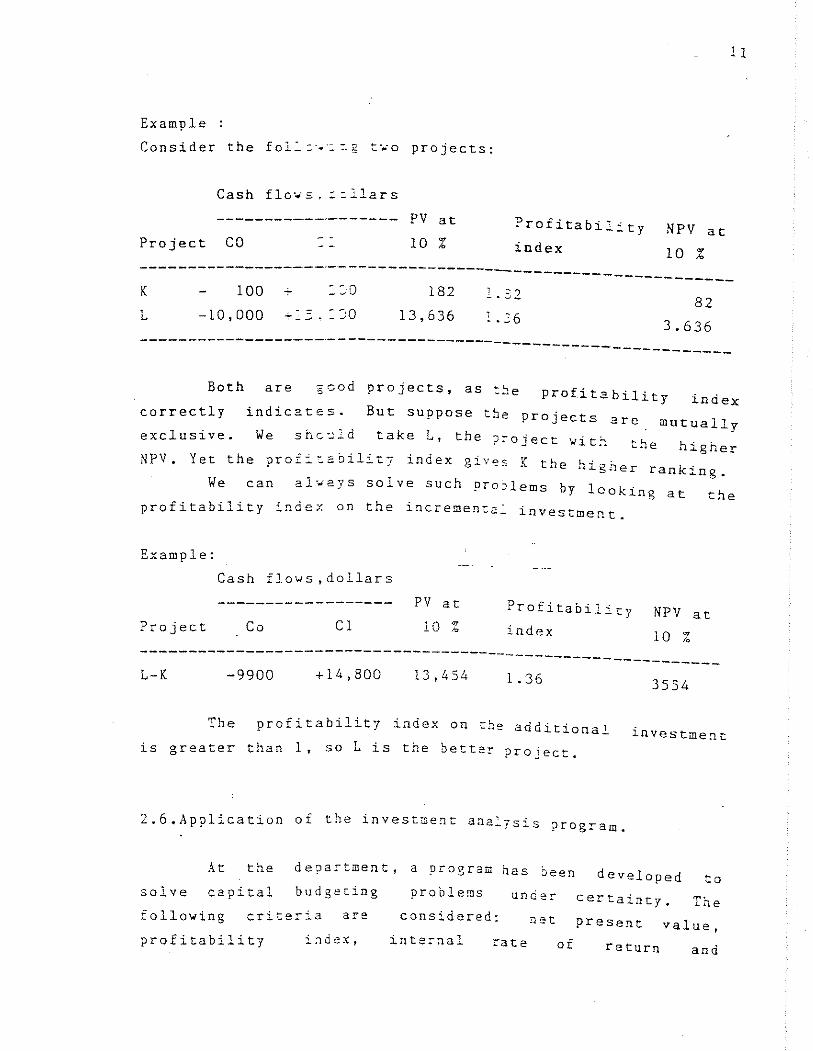
Example :
Consider the fol::"~:i t~o projects:
Cash flo·.'s. ~ :llars
Project CO
PV at
10 % ?rofitabil:'ty
index NPV at
10 %
11
------------------------------------------------------------K 100 ::"0
L -10,000 -~ = JO
182
13,636
1 :- '? - . -' ....
! .26 82
3.636 ---------------------------------------------------------
Both are 5 cod projects, as :~e profitability index correctly indicates.
exclusive. We shG~ld take L, the ?~oject ~it~ the higher
NPV. Yet the prof:':abilit7 index gives K the higher ranking.
We can always solve such pro~lems by looking at the
profitability index on the increment2~ investment.
But suppose tbe projects are mutually
Example:
Cash flows,dollars
Project Co Cl
PV at
10 % Profitability
index NPV at
10 % ------------------------------------------------------------L-K -9900 +14,800 13,454 1.36 3554
The profitability index on the additional
is greater than 1, so L is the bette~ project. investment
2.6.Application of tbe investme~t ana:ysis program.
At the department, a program has been developed to solve capital budgeting under Certainty. The following criter::'a are!
problems
considered: net present value, profitability inte:-nal rate of return and

12
(discounted) payback period.
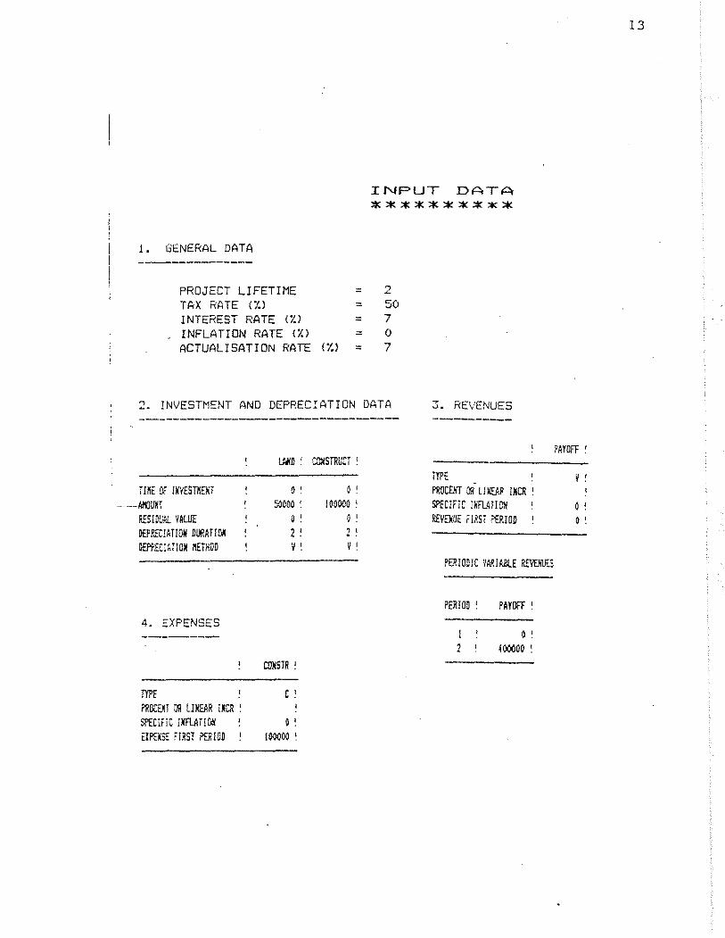
Figure 2.6 is based on example 2.1 ~tax effects are
also considered now) and illustrates input and output data.
The program allows several depreciation
different
concerned,
types
not
of revenues and expenses.
schemes and
As output is
only the investment criteria are given, but
also a detailed picture of the periodic cash flows.
1. GENERAL DATA ----------
PROJECT LIFETIME TAX RATE ( %) INTEREST RATE (;.)
INFLATION RATE (I.)
ACTUALISATIoN RATE
= = = =
(;. ) =
INPUT DATA **********
2 50 7 0 7
2. INVESTMENT AND DEPRECIATION DATA 3. REVENUES
Tm Of jrIESTl!E~,
--··AI()L~l
P£SJ WAL 'IAWE O£PP.ITlATlOW DOOATlM DEP!'£CrmOH XETHOD
4. EXPENSES
TYl'f ?IUlCE!! OR ll~R iXCR ! SPfC~FiC IKFlATlOH EllUl: fIRST ?SHOD
lM'D ~
o ' 50000 '
o ~ 2 ! ~ !
COlIS,R !
r , " .
o ! 100000 '
CD:/STRUCT '
o ~ 100000 '
o ' 2 ! V '
-------
TYPE PROWIT OR ll)(SlR 1 XCR ' SPECIfiC lliFUTION REVElWE FJRSi i'EP.lOD
PERIODIC '1A!1JI.liU Rfl'ElllF.3
PERIOD !
I 2
PAYOFF !
o ' HIOOOO '
13
PAYOFF'
o ! o '

PERIODIC DEPRECIATIONS
PERIOD'
1 1
LAAD! CCXSTRUCT!
o ! o ! o ! o !
15

1. EVALUATION CRITERIA
PROJECT LIFETIME 2 TAX RATE ::.0 ACTUALISATrON RATE 7
NET ?'RESENT YALUE PROFITABILITY INDEX INTERNAL RATE OF RETURN PA)'8AQ( PERIOD
PERIODIC FLOWS
OUTF"UT DATA *********'*"*
WITHOUT TAXES
18574 1.124 11.96 1.929
WITH TAxES
-~11S .562
NEGATIVE > 2
PO/II! """" """" ! [l'{11T!/E I !'O'm:TA- I fRHAI Tim ! If!U ru ' CASI! P J:w ~
''"'' " o ' " o ' 100000 ~ -l~!
""'" . 1000») ! ;~~
PERIODIC R£VENUES
. ' -, 4. PERIODIC EXPENSES
nlJOS PR!llT "",n , , ' , ' "
, , " " -1@lQ1 ..,..., --. -~' , ' ~~ 1~1. l~~ l~~
:""'- 11O"' ! rAIB ;,! EU2I or Wv~
, ilJlI
I~I " " -l~'_ .. " , ' ~! " j' , ' !~!

Chapter 3.
CAP~TAL RATIONING UNDER CERTAINTY
3.l.DefinitiDn
The capital budgeting prDblem involves the allocatiDn
of scarce capital resources amDng cDmpeting eCDnomically
desirable projects, nDt all of which can be carried out due
to a capital (or other) constraint. This problem is referred
to as capital rationing.
is often that the restriction on the supply of
b.ottlenecks capital reflects non capital constraints or
within the firm. For example, the supply of key personnel to
carry out
restricting
Similarly,
Df
the projects maybe severely limited, thereby
the dollar amount of feasible investment.
consideration of management time may preclude the
programs beyond some level. This should more adoption
properly be called lahor Dr management constraincs rat.her
than capital cons~raints. These restrictions limit or
the maximum amau'nt of investment which can be undertaken by
the firm.
Many firms capital constraints are soft. They ~eflect
no imperfection i.:1 the capital market. Instead they are
provisional limits adopted by management as an aid to
fin2ncial control. Soft rationing should never cost t~e firm
If capital constraints become tigh~ enough to
hu:-:, then
constraints ..
the firm raises mDre money and loosens
But what if it cannot raise more money-what
the
if
it :aces hard rationing?
Hard rationi~g implies market imperfect~on-a barrier
be:'""'een the firm and capital markets. If that barrier also
that the £:~mts shareholders lack free access to a
wel:-runctioning ca?ital market, the very foundacion of net
present value crumble.
16

3.2.Structure.
The entire discussion of methods of capital
rests on the proposition tha t the wealth of
17
rationing
a firmts
shareholder is highest if the firm accepts every projects
that has a positive net present value. Suppose, however,that
there are limitations on the investment program that prevent
the company to undertake all such projects. If this is the
case, we need a method of selecting the package of projects
that is within the company's resources yet gives the highest
possible net present value.
We will survey several techniques which are applied
to the capital budgeting problem setting, under conditions
of certainty and under conditions of risk
- Capital rationing under conditions of certainty:
Lorie and Savage proposed profitabi~ity index
techniques for the single period case and the multi
period case. Weingartner formulates th-e capital ratloning
problem
model.
Since
advances
to the
model.
first as an LP theh as an integer programming
these pioneering works, there have been many
in the area of mathematical programming applied
capital budgeting problem, e.g. goal programming
Capital rationing under condi~ions of uncertainty
(see c.hapter 5).
3.3.Profitability Index.
Lorie and Savage proposed a solution to ~he capital
rationing problem for the single period case and the multi
period case, on the assumption that

18
l. The timing and magnitude of the cash flows of all
projects are known at: the outset with complet2
certainty.
2. The cost of capital is known (independent of the
inve~tment decisions under consideration) so that the
present value of all the projects are also given.
3. All projects are strictly independent, i.e.the execution
oi one project does not affect the costs and beneiits or
some other project:.
Under these simplifying assumptions our problem
becomes one of how to selec:: among projects which ha,"e
positive net present values.
For a single period case, the solution is to rank all
projects by the profitability index and then select from the
top of the list until the budget is exhausted. The ?rocedure
is simple and easily understood. However, it depends
set of very limiting and unrealistic assumptions:
on a
name!.y
that cash flows are known, the eost of capital is
independent of the investment decision, mutually excl usi \'e
projects are ruled out; and all outlays occur in a single
period of time so that the budget constraint applies
single period.
Lorie and Savage drop the latter restriction by
considering
limitation
the selection process in which
occurs in more than one ?eriod~ Like
the
also
to a
also
budget
many
seminal articles in finance and economics it is the question
they asked, and not the par~icular solution which they
proposed, which is of lasting interest.
Example
Lorie and Savage consider the followi~g example:

Project /
1
2
3
4
5
6
7
8
9
Suppose
NPV
14
17
17
15
40
12
14
10
12
the
are selected,
Cash. outflow
in period 1
12
54
6
6
30
6
48
36
18
budget is 100. This
and the budget used
PI
1 • 167
0.314
2.83
2.5
1.33
2.0
0.292
0.277
0.666
means projects
is 98.
3.4.Mathematical Programming: Linear Programming.
19
Ranking
5
7
1
2
4
3
8
9
6
3,4,6,5,1,
By the linear programming(LP) the firm can examine
very large-scale choice problem in which the number or
alternatives is virtually unlimited in the relevant range.
It helps allocating and evaluating scarce resources and
provides decision makers .... ith some very insightful
information regarding the ~arginal value of resources.
The LP formulation of capital rationing is as follows:
fI max NPV = I OJ xJ
(1)
J>' II
s.t I C v ~ K, t=l,2, ... T (2 ) Jt
., J
J"
0 ~ v " ~J - 1 ( 3 )
XJ
= percent of projec~ j that is accepted
bJ
= NPV of project j over its usef~l life

.I
CJ~ = cash outflow requireC: by project
Kt = budget available in year t
in year t
The following aspects should )e noted about
problem formulation above:
20
the
1. The x J decision var~ables are assumeQ to be continuous-
that is, partial projects are a~lowed in the LP formulation.
2. The usual nonnegativity constant or L? is modified as
shown in equation(3) to also show an ,oper limit for each
project.
3. It is assumed that all the input par=.neters - DJ ,C J' .K~
,are known with certainty.
4. The b J parameter shows the NPV of project over its useful
life. where all cash flows are discounted at the cost of
capital, which is kno~n with certainty.
The marginal value to the ::c~ of the budget
constraints are obtained by comparing the total NPV with and
without an extra dollar of resources. In .L? such values are
referred to as dual 'lariables
represent the opportunicy costs
firm's resources~
or s~adow prices.
of us:~g a unit of
~. .. ney
~he
The dual LP formulation for the cap~:al ~3tioning proble~ is
as follows
K II
Min I P~ Kt + I YJ t .. t J., s. t
(a)
V
I P, Cjt + \l j ~ ':J. j :;;;lt2,.",~~ ,., .; ( b )
P" IJ) ~ 0 t =1 2 , l' =1 , .N ( c )
• • . . • - j . - , . where:
P.,. = dual decision va~iable whic~ re?::-esent3 the cost.
associaced with resource of type t.

21
/ .-IJ = dual decision variable associated with project j.
The dual formulation has important implications for
the financial manager. Namely, the dual L? and its optimal
solution provide valuable information for both planning and
control functions in the capital budgeting
This optimal solution gives the shadow
accepted and rejected projects.
decision process.
prices for the
These values enable the decision maker to rank all
projects according to their relative attr3c~iveness.
under
For accepted projects
the slack variables ( S,,) the shadow prices are found
for the following constraint:
The shadow prices are computed using the following
expression
= shadow price associated with accepted project
(shown under the slack variable associated with
project j)
= NPV for project j shown in the objective function.
p: = shadow price in the optimal solution associated with
each resource t which is required to accept a
project. (shown under the slack variable associated
with the corresponding resources).
C[\. = quantity of
j .
resources of type t required by project
The shadow prices YJ
may very well give a ranking for
the projects which di£fe~s from that given by any of the
simple models as payback, NPV, IRR,or the profitability
index. Such differences in ranking will exist because the
latter models look at projects independently.

,/
22
The shadow pric.es show interrelationships among
projects by means of the budget constraints. They evaluate
the projects at cost of capital ( p~) that is implied by the
optimal use of resources of type t.
For the rejected projects the shadow prices are
computed in an analogous way as for accepted project.
llJ = T
I P'" ,
= shadow prices associated with rejected project
j (shown in the objective function row in the column
for x J ).
The llJ value shows the amount by which the objective
funtion would decrease if the firm were forced to accept the
unattractive
would mean
project
that the
j. If such projects were accepted,this
scar~e capital budget dollars would be
used in a suboptimal way, since the- opportunity cost
with the cash outflows C-Ip" c.,\:---) exceeds , . associated the
present value of the benefits generated by the projects.
It should be mentioned that the values must be zero
for all projects that are accepted (including partially
accepted projects) because the benefits of these projects
must justify the cash outlays in the various periods of the
planning horizon (C)~ ) when they are evaluated at the
implied cost of capital ( p~) when the budgets each year are " llsed in an optimal way~
Example:
Lorie and Savage nine-project problem.

Project NPV
1 14
2 17
3 17
4 15
5 40
6 12
7 14
8 10
9 12
Cas.h outflow
in period 1
12
54
6
6
30
6
48
36
18
Budget available I c.Jx) ~50
The LP formulation is as follows :
Cash outflow
in period 2
3
7
6
2
35
6
4
3
3
Max NPV ~ 14x, + 17x~ +17x~ +lSx~ +4Cx r +12xb
s • t •
, 1 " ..... T.l."' .... '3
12x, + 54x, +6x l +6x ... +30x s
+6x& +48x, +36x& +18x~ ~ SI ~ 50.
3x, + 7X, +6x, +2x.., +35x,.
+6x, +4x 1 +3x 8 +3x, + 5,
x, + S:; ~ 1 x., + S , ~ 1
x, + S ... ~ 1 x, 51 ~ 1
X 3 + S 5' = 1 x '" + Sa = 1
::: 20~
x1 + S"
x& .;- S '\0
x, .;- S"
x S ) 0 i ::;; 1 ,2 t .. ,11. J
, ~ • j ::;; 1 f 2 , ,9.
= =
=
budget constraint
year 1
budget constraint
year 2
1 Upper limits
1 on project
1 acceptance
Non negativity
constra.int
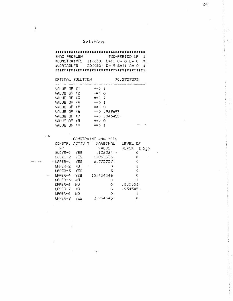
23
The problem has been solved with a package on Apple
II developed at the department.
24
5olu·hon
ttlttttttttttttttlllllllltltttttl'ttttt lMAX PROBLEM TWO-PERIOD LP 1 tCONSTRAINTS 11 «30) L=ll G= 0 E= 0 i ,VARIABLES 20«80) D= 9 S=11 A= 0 1 tttfftil1itttllittltltlltlllttttttttt'l
OPTIMAL SOLUTION 70.2727273 --------------------------VALUE OF Xl ;:::;=;. 1 VALUE OF v.,
"~ ==.;. 0
VAl.UE OF v_ "" ::=::>
VALUE OF X4 :::=> 1 VALUE OF X5 => 0 VALUE OF X6 ==} .969697 VALUE OF X7 =} .. 045455 VALUE OF XS ==;- 0 VALUE OF X9 ==>
--CONSTRAINT ANALYSIS
CONSTR .. ACTIV ? MARGINAL LEVEL. OF NR VALUE SLACK Ui)
8UDYE-j YES .. 1:6364 -- ()
BUDYE-2 YES 1.863636 0 -tJPPER-l YES 6.77:727 (l
UPF'£R-2 NO 0 UPPER-3 YES 5 0 UPPER-4 YES 10.454546 0 UPPER-5 NO 0 1 UPPER-6 NO 0 .030303-UPPER-? NO 0 .. 954545 UPPER-8 NO 0 1 UPPER-9 YES 3.954545 0

25
We see that the basic variables, that is f the
variables that are equal to a positive value in the ~pt=-mal
solution are ! x." x~, x~, x" x 1 , x~ (column value or x)
and S."S1' S" S~, S,o (column level of slack).
Any of the variables in the problem which are equal
to zero, are in fact, non basic va~iables in the opt:.mal
solution. Thus, X 1. = xI" = xa = 0, which shows that these
three projects should be completely rejected; in addition
S,= S~ = 0, shows that the entire budget of 50 in year 1 and
20 in year 2 has been spent on the six projects that have
been designated lor acceptance. Further-, S; = Ss- = S6 = S" = 0, since the project corresponding
100% accepted.
to these slack
variabl~s have been
These projects require the use of the entire budget
in both years and generate the maximuQ objective func~ion
value of 70,2727273, which is the NPV of the accepted
projects.
The marginal value of const~aint ~umber 1 (the shadow
price of s, ) is O~136364 which means that the object:"ve
func~ion would increase by this amount (b.136364) for each
dollar of additional budget they could obtain.
constraint is active because any changes in tha cons~raint
can change the objective function.
The same explanation can
conseraints.
be used
LP models seem tailor-made :or
for the other
solving capi'L.al
budgeting
they not
problems when resources are 1~3ited. Why then are
universally accepted either in theory or in
practice? .One reason is that these models are often not
cheap to use. LP is considerably c~eaper in terms of
computer time, but it cannot be used when large t indiviSible
projec'L.3 are involved.
As with any sophisticated long-~3nge planning too 1
there is the general problem of getting good data. It is not
just worth applying costly, sophisticatad methods for poor

26
data. Furthermore, these models are based on the assumDtion
that all future investment opportunities are known. In reality,
process.
the discovery of investment ideas is an unfolding
Before we leave the area of linear programming a
appropriate LP noteworthy controversy relative to the
formulation should be mentioned. Under capital rationing,the
appropriate discount rate to use in determining the net
present values of projects under consideration cannot be
determined until the optimal set of projects is determined,
so that
well as
the size of the capital budget is ascertained as
the sources of the subsequent finanCing and hence
the cost of capital (or the appropriate discount rate to use
in calculating NPVs). This is a simultaneous problem wherein
the firm· should concurrently determine through an iterative
mathematical programming process bot~ the optimal set of
capital projects and the optimal finanCing package, with its
associated cost of capital to be used in the discounting
process.
Weingartne~ suggested an operational approach; his
model assumes %hat a:1 shareholders have the same linear
utility preferences for consumption~ And it makes the period-
by-period .utilities iadependent of one another. He t.hen
proposes
dividends
a more operational mode1 1 which maximizes the
to be paid in a terminal ye~r, where throughout
the planning horizon dividend are nondecreasing and can be
required to achieve a specified annual growth rate. Over the
past decade, several other authors have jumped into the
c~n,troversy, each suggesting his own reformulation.
The Weingartner 1 s basic horizon model is as follows
Max Z = -; 11, x J i- v, - w_ - ,
J s • t •
.1 a 'J J
Xl i- v, - w, 1. - D, (a)

27
~ a'l X J - (l+r)v t •. 1 + v .. + (l+r)w •. , - WI. 1. D"
t = 2, •• o,T ( b )
j:::;: l, .... ,n ( c )
t = 1, .•• ,T ( d )
where: ~ value of all cash flows of project j subsequent to a J =
the horizon discounted to the horizon at the market
rate of interest, r •
x J = fraction of project j accepted.
T = horizon year.
vt = amount available for lending in period t .
w ... = amount borrowed in period t.
a 'J = cash flow in period t from project
j.(pos-expenditure!outflow, neg-revenue/inflow)
D t - anticipated cash t~row-off in period t.
The dual of the basic horizon model is as follows:
T n Min p. D-t, +
s. t
2. J' ,
,. J.., p. j =l, ... ,n .. (1)
~ 1 ( 2)
). -1 "
(3)
p. .. , - O+r)p. ,. 0 • (4)
;;. 0 • t -2 ••••• T ( 5 )
( 6 )

28
The following derivations help to understand the meaning of
the dual variables
(2)and(3) Po'" = 1 (7)
(4)and(5) p:- ,
(1+r) (8) = f\
(7)and(8) P+..~ = (1+r) f: ~~ (1 +r) ,
.. = ft. >.
= i-l f~ (l+r) t + r-t.
= (l+r)r-~
So, one can see that f. is the compounded rate of
interest which expresses the yield at the horizon of an
additional dollar in year t.
• When a project is
corresponding restriction
fully accept.ed ,- that: is, x_ = 1 J
of the form of (a) becomes
.-t,P~a"J
~
= a J
,. T_ t
+ I (-a,,)(1+r) ~
= a J t: "'-.
This is the value of the projec~ a~ time T. This
the same as saying that the NPV of the ?roject should
positive.
...
,the
is
be
For the rejected project we know that x J = O,and also ~ • ~ 11 x J ' i, and therefore ,oJ = 0.
This is the same as saying that the NPV is smaller than O.

29
3.S.Integer programming .applied
problem.
to the capital rationing
The main mocivations for the use of IP in the capital
rationing problem setting are the following
1. Difficulties imposed by the acceptance of partial
projects in LP are eliminated.
2. All the project interdependencies can be formally
included in the constraints of ILP, while the same is not
true for LP due to the possibility of accepting partial
projects.
In using the simple capital budgeting models
(NPV,IRR,PI.etc) it is assumed that all the investment
projects are independent each other (i.e.that project cash
flows are not related to each other and do not influence or
one another if various projects are accepted). In change
using ILP, virtually any project dependencies (mut:lally
exclusive, prerequisite, complementary) can be incorporated
on the model.
The general ILP formulation for :he capital rationing:
N
Max NPV = l . j-1
st
t=1,2, ..... T
j=1.2 •••• N
There are three types of project dependencies:
a. MutuallY exclusive projects.
A set of projeccs wherein the acceptance of one project
in the set includes the simultaneous acceptance or any
other project in the set. It is incorporated in the model
by the following constraint:

J
l.. x ~ 1 J.;:.J
~ set of mutually
consideracion
30
exclusive projects under
jb:J ~ chat project j is an element of the set of mutually
exclusive project J.
This constraint states that at most one project from set
J can be accepted; this means that the firm could choose
not to accept any project from set J. On the other hand,
if it was necessary to select: one project from the set,
the above contraint would appear as a strict equality
2.. X' ~ 1 jE.J J
b. Prerequisite/contingent projects.
Two or more projects wherein the acceptance of one
project (A) necessitates the prior acceptance of some
other project(s) (Z):
x"" ~ X '1..
If project A cannot be accepted unless project Z is
accepted, we could say that project Z is a prerequisite
project for acceptance of- project"-A; alternatively, we
could
upon
say that the accept:ance of project A is contingent
the acceptance of project Z. However project Z can
be accepted on its own and project A rejected.
c. Complementary projects.
Wherein the acceptance of one ~rojec~ enhances the cash
flows of one or more other projects.
There are t~o complementary projects,7 and 8. Either of
these projec=s can be accepted in isolation. However, if
both are accepted simultaneously : the COSt will be
r~duced by say 10%. The net cash inflow will be increased
by 15%. To handle the problem, a ne~ project (project 78)
would be constracted. The constraint below is needed to
preclude acceptance of both projects 7 and 8 as well as

78; because the latter is the
consisting of the t~o former projects.
xl + x 8 + x r8 ::i 1
The shortcomings of the ILP:
31
composite project
a. ILP is probably only feasible for small to medium size
capital budgeting problems (25 constraints and 100
projects).
be paid
We have to think whether the price that has to
in moving to ILP from LP is worth the benefit
gained.
b. 'leaningful shadow prices (which show the marginal change
in the value of the objective function for an incremental
change in the right hand side of various constraints)
are not available in ILP. That is, many of the
constraints on ILP problem which are not binding on the
optimal
of zero,
integer solution
whic!) indicates
will be assigned shadow
that these resources are
prices
"free
goods fT• In reality this is not true since the objective
function would clearly decrease if the availability of
such resources were decreased.
Example:
Consider the following 15 projects

32
Cash outilows
P,oject Clj C2j Cj NPV
------------------------------------------------------------1 40 80 0 24
2 50 65 5 38
3 45 55 10 40
4 60 48 8 44
5 68 42 0 20
6 75 52 20 64
7 38 90 14 27
8 24 40 70 48
9 12 66 20 18
10 6 88 17 29
11 0 72 60 32
12 0 50 80 38
13 0 34 56 25
14 0 22 76 18
15 0 12 104 28
Budget
constraints: L CljXj~300; L C2jXH540; Z C3jX] ~380
Project interrelationships :
1. Of the set of projects 3, 4, and 8, at mos~ two can be
accepted.
2. ?rojects 5 and 9 are mutually exclusive, bu: one of the
two must be accepted.
3. ?roject 6 cannot be accepted unless both projects 1 and
14 are accepted.
4. Project 1 can be delayed 1 year, the same cash outflows
will be required, but the NPV will drop to 22.
5. Projects 2 and 3 and projects ]0 and 13 can be combined
into complementary or composite projects wherein total
cash outflows will be reduced by 10% and NP'/ increased by
12% compared to the total of the separate projects

33
6. At least one of the two composite projects above must be
ac~epted
Solu1:~on:
Maximize NPV :
24:>::, + 38X .. + 40X!J + 44X .. + 20X s + 64X, + 27X, (a)
+ 48X8 + 18X .. .;. 29X,0+ 32X,,+ 38X".+ 2SX,"!> + 18X, ...
+ 28X,\"+ 22X.,.+ 87 • 36X<7 + 60.48X,8
subject to
40X, + SOX. + 45X, + 60X .. + 68X ... + 75X. + 38X7 (b)
+ 24X8 + 12X~ + 6X,0+ 85.5X'7+ 5.4X,8 ~ 300
80X, + 6SX,,- + 55X 5 .,. 48X.., + 42X ,.- + 52X ~ + 90X -r + 40X e + 66X ., + 88X,o + 7 2X" + 50X,>.+ 34X .. ~
- + 22X '\"i + 12X,s-+ 40X ". + 108X'7+ 109.8X,8
5X, + lOX 3 + 8X", + 20X" + 14X 7 + 70X8 f 20X,
+ 1 7X 10 + 60X.n + BOX "1'1.,. + S6X 1~ + i6X-1 "'t + to"ttX 1~
v X., + Xi ~ 2 -' I
X ,+ v A":j ~ 1
2X to ~ X, + X' ... ei'cher constraint (g) or
2X ~ v
H2o+" X, .. (h ) must be satisfied " A
X , .,. X 1(, ~ 1 v + v X17 ~ 1 -'2 A> v A f~ +- X,~. + X,g i. 1 v A~? +- X18 S 1
Xi. ~ [0,1] i ~ 1 , ? . . . , 18 - ,
~. 540
~ 380
(c)
(d)
(e)
Cf) (g)
(h)
( i)
(j)
(k)
(1)
(m)
X 16 is a decision variable to denote the delay of project
for 1 year

34
X 11' is a decision variable to denote the acceptance of
the composite of projects 2 and 3
X 18 is a decision variable to denote the acceptance of
the composite of projects 10 and 13
3.6.Goal Programming applied
problem.
to the capital rationing
Under conditions of certainty and perfect capital
the selection of the set of capital projects that market.s,
maximize NPV will guarantee maximization of shareholder's
wealth or utility.
However, if capital market imperfections exist (such
as capital
rates, etc)
rationing, differences in lending
then the maximization of NPV may
and borrowing
very well not
lead to the maximization of shareholders' wealth.
addition,
motivated
investors and managers are interested in
by several objectives as follows
stability of earnings and dividend per share;
growth
growth
In
and
and
in
sales, market share and total assets; growth and stability
of reported earnings or accounting profit; favorable use of
financial leverage; and return on sale, equity and operating
assets.
Thus anI y a model that incorporates mul~iple
c.riteria as objective can be a robust, yet. operational,
representation of the pluralistic design environment found
in real-world capital budgeting problem setting.
Goal programming is such a multi criteria model. It
is capable of handling decision situations which invol ve a
Single. goal or mUltiple goals. Frequently the multiple goals
of a decision maker must be measured by different
standal"ds. Often one goal or set of goals can be achieved
only at the expense
progl"amming allows
of other goals or set of goals.
for an ordinal ranking of goals so
Goal
that

35
lo~ priority goals are considered only after higher priority
goals have been satisfied to the fullest extent possible.
The general Goal programming (GP) model.
The basic assumptions underlying the LP model are
also valid for the GP model. The significant difference in
structure is that the GP does not attempt to maximize or
minimize the objective criterion directly as does the LP
model. It rather,seeks to minimize the deviations bet· .. een
the desired goals and the actual results according to the
priorities aSSigned. The general GP model is expressed as
follows
It'
Min I (di+di)
s. t .. n
I J>1
~here
8ij x j
. b .
1.
xJ,di,di ~ 0
i==l, ..... ,n
d represents degree of over achievement of a goal.
d represents degree of under achievement of a goal.
i goals
bi~ target value.
GP will move the values of the deviational variables
as close to zero as possible within the environmental
constraints and the goal structure outlined in the model.
Example:
The
GP Formulation and Solution of the Lorie-Savage
Problem
same fir~ that ~as evaluating the nine projects
now feels that the NPV objective should be supplemented with
four other goals ~hich reflect the short-run attractiveness
of the projects. Specifically, the firm feels that stability
and growth in sales as well as net income are very important
vehicles to assist. the firm in maximizing shareholders'
wealch.

36
The following table shows the contribution that each
of the projects will make to net income and sales growth in
the next 2 years.
Net Income Sales Growth
Project Year 1 Year 2 Year 1 Year 2
------------------------------------------------------------1 2.0 4.0 0.02 0.03
2 2.0 4.2 0.01 0.03
3 1.6 2.5 0.02 0.02
4 1.2 2.8 0.01 0.02
5 3.0 5.0 0.03 0.04
6 1.1 1.4 0.01 0.01
7 1.5 3.0 0.01 0.02
8 1.2 1.8 0.01 0.015
9 1.3 2.4 0.01 0.018
The firm wants to achj.eve net income levels of 8 and 16,
respectively, lTI years 1 and 2, and sales growth of 0.08 in
each year, as well as to maximize NPV.
Two objectives are considered
1. Placing the net income goals on priority 1, the sales
2 •
g.oa13 on priority 2, and the ~PV goal on priority 3; on
the first two priority levels the year 1 goals should be
weighted twice as importantly as the year 2 goals.
All £ i ve goals placed on priority level 1 but wi ttl
relative weights of 10 for net income in year 1 , 2 for
net income in 2,5 for sales growth in year 1 , and 2 for
sales growth in year , " , and 1 for }iP'l.

37
Solution:
The GP formulation is a~ follows:
X 1
X ~
12X, + 54X~ + 6X 3 + 6X" + 30X~ -+- 6X b
+ 48X 7 + 36X6' + 18X 9 + S, = 50
Budget constraint year 1
3X 1 + 7X .. + 6X:I + 2X ... + 35X ... + 6X ..
+ 4X 7 + 3X B + 3X"l + S ~ = 20
Budget constraint year 2
+ S3 = 1 X" + S ~ = 1 XT + S 9 = I Upper limits
+ S" = 1 X S" + S 1 = 1 Xe + S 1O = 1 on project
X 3 + S ,- = 1 X 4 + S B = 1 X9 + S 11 = 1 acceptance
j = 1 , 2, ,9 Nonnegativity
X j , Si ~ 0 i = 1 • 2 , ,11 constraint
2X, + 2X,- + 1.6X 3 + 1.2X", + 3X, + 1.1X b Net income
+1.5X7 + 1.2X8 + 1.3X"j + d1 d1 = 8 year 1
4X + 4.2X + 2.5X + 2.8X + 5X + 1;4X Net income
+3X + 1.8X + 2.4X
0.02X, + 0.01X 2 + 0.02.'::; + O.OlX.,
+ 0.03 X' 10 + O. 01 X 6 + O. 01 X 7 + 0.01 x 8
+ O.OIX~ + d; - d; = 0.08
0.03X, + 0.03X2. + 0.02X J + 0.02X""
+ 0.04X, -;. O.OlXi, + 0.02X 7 + 0.015X8
+ 0.018X 9+ d~ - d; = 0.08
year 2
Sales growth
year 1
Sales growth
year 2
14X, + 17X,- + 17X} + 15X", + 40X, + 12X. + 14X 7
+ 10X8 .,. 12X'l + d~ - d~ = 40 NPI(

Notice again that the goal level for the NPV goal i,,<:J
arbitrary achievable value.
The two objective functions are as follows:
1. Minimize weighted deviations =
P 1 ( 2d;- + d'; ) + P,.( 2 d; + d':;; ) + P;; ( d ~ + d; )
2. Minimize weighted deviations =
P,(10d; + 2d; + Sd; + 2d~ + d~ - d~)
The optimal solution for the two objestive functions are:
Objective function 1
Project
acceptance
Goal levels
achieved
---------------------------------------------------~--------
x, = 1.0000 7.231 Net income year 1
,X t 0.0426
X3 = 1.0000 13.209 Net income year 2
X.., = 1.0000
X, = 0 0.0699 Sa'les growth year I
X" = 0.9504 -
X7 = 0 0.0988 Sales growth year
XI? = O.
X" = 1.0600 70.129 NPV
Objective function 2

Project
acceptance
x, = 1 . 0000
Xt. = a X3 = 1.0000
X-'1 = 1 .0000
X, = 0
Xi, = 0.9697
X7 = 0.0455
Xa = O.
X", = 1.0000
Goal levels
achieved
7.235
13.194
0.0702
0.0986
70.273
3S
Net income year 1
Net income year 2
Sales growth year 1
Sales growth year 2
NPV
The optimal LP solution showed 100% acceptance of
projects 1.3.4 and 9, as well as 97% acceptance of project 6
and 4.5% acceptance of project 7,which generated an NPV
level of 70.273. All the GP solution above also accept 100%
of projects 2,3,4 and 9. The only difference among the
solutions is in the area of the partially accepted projects.
In the first G? solution (objective function 1) project 2
enters into the solution because of its contribution to- tile
achievement of the new goals in the GP formulation.
The other GP solution is virtually the same as the LP
solution. 'Greater variation in the optimal solution would
probably have been found if more projects were under
evaluation and/or greater diversity of goals were included
in the formulation.

Chapter 4
CAPITAL BUDGETING UNDER UNCERTAINTY.
4.l.Sensitivit7 analysis/break even analysis.
will
Uncertainty means
happen. Therefore,
that more things can happen tha:
whenever we are confronted with
cash-flow
happen. If
find that
forecast, we should try to discover what else caj
we can identify the major uncertainties, ve rna;
it is worth undertaking some adtitiona,
preliminary research that will confirm whether the ?rojec:
is worthwhile. And even if we decided that we have done aI'
we can to resolve the uncertainties, we still want to be
aware of the ?otential problems. We do not want to be caugh'
by surprise if things go wrong~ we want to be ready to tak(
corrective action.
Companies try to identify the principal threacs to
project's suc~ess. The simplest way to do it is to undertakl
a sensitivity analysis. In this case the manager consider!
in tura each of the determinants of the project's succes!
and estimates how far the present value of the project WQul(
be altered by taking a very optimistic view of tha t.
variable.
Sensitivity analysis or this kind is easy, but it i~
not always helpful. Variables do not usually change onp. at <
time4 If costS are higher than we expec~, it is a good be~
that sales volumes will be lower.
Many companies try to cope with this problem
examining the effect on the project of alternative plausiblt
combinations of variables. In other 'Words, they wiI:
estimate
different
case.
the net present value of the project
scenarios and compare this estimate with the
und e:r
bas ~
In a sensitivity analysis we change variables one a:
a time: when we analyze scenarios, we look at a limite'
40

41
number ot alternat~ve co~binations of variables.
Sensitivity analysis Jails down to expressing cash
flows in terms of unknown var~ables and then calculating the
concequences of misestimating the variables. It forces the
manager to identify the underlying variables,indicates ~here
additional information would be most useful, and helps to
expose confused or inappropriate forecasts.
One drawback to sensitivity analysis is that it
always
exactly
gives
does
some~hat ambiguous results. For exam~le,"'hat
optimistic or pesimiscic mean? The market.ing
depar'tment :nay be .interpreting the cerro in a different
from the production devartment.
When we undertake a sensitivity analysis of a project
we are ask~ng. how serio~~-it ~ould be if sales on costs turn
out to lie worse than we forecasced. Managers sometimes
prefer to rephrase this question and ask how ~ad sales can
get. before the project begins to lose moneY4 This is kno',./n
as break even analysis.
The break-~ven point is locaced ~here t~e ~otal cost
curve i.!1t2rsects =he total revenue curVe, or equi.?alent.ly
·,.,.here t:ctal '""Tevenue ~e:-quals tOLal cost.. Convent.ional hreak-
even analysis 'represents t..oLal revenue and i::ot:al Cost
scraight li,nes. This assumes ~hat output and sales can be
iilcreased . without changing ?r~ca (at. least, ~he ~£f~c.t. of
price changes are ~ot shown) and t~ac t~e f~=~ operates al:
the same efficiency at all le'rels. T:1US, t:o inc:::'ease profit
it is rrecessary merely to inc=ease t~e number or units sold.
Exam'ple :"
Suppose a f~r~ Ls 91anning to buy a 3umer~cal control ,
for 50,000. It is ex?ec~ed' to be used for 5 years and have
receipt:s of 15,000; 15,000; L:;,OOO; ~4,500 and l"-OOO ac t!1e
end of eac~ year.
It is t-ne, company' s policy to use a 11: :ni.r1i.:num att.::act:::'ve
Management. wants e:O conduce: a sensi:ivi~1 analysis

42
respect to error in the forecast of initial investment,1if~
time, end or year receipt and minimum rate of return.
Solution:
The solution to this problem was solved by a program
developed for this purpose. The dicussion of this program
and the solution to this problem can be seen in chapter 6
4.2.Decision trees.
A that has been recommended to handle
complex,
technique
sequential decisions over time is the use of
d ecislon trees.
A decision tree is a formal representation of
available decision alternatives at various points through
time which Bre followed by c~ance events that may occur with
some probability. A ranking of the available decision
alternatives is usually ac~ieved by finding the expected
returns of the alternatives, which merely requires
multiplying the returns earned by ea~h alternative for
various chance events by the probability that the event will
occur and·summi~g over all possible events.
Managers may be tempted to think only about the ~irst
accept-rejec: decisions and La ignore the subsequent
investment decisions that ~ay be tied to it. Bu c if
subsequent investment decisions depend on those made toda.y,
then today's decision may depend on what we plan to do
tomorrow.
Of course, it would be imprudent for the fir:;, to
immediate~y impleme~t the project with the higest expected
return. This optimal ac:::'on with ·the unidimensional
cr:':'erion c::-ies out for £ur~jer analySis. Namely we should
investigate the following
1. The degree to which the estimated probabilities of the
various states of the economy would have to change for

43
the optimal solutio~ to no longer be optimal.
2. The
the
extent to which the estimated returns associated with
alternatives and states of the economy would have to
change in order to shift the optimal decision.
3. The
4. The
degree of risk associated with lack of alternatives.
utility that the firm attaches to each Of the returns
for each of the states of the economy based on the firm's
goals, risk, posture, risk-return preferences and so on.
Thus decision tree analysis is advocated as an
initial step which requires further analysis rather than the
final word in the firm's effort to maximize shareholder's
expected _utility
Example:
A firm is considering three alternative single-period
investments, A, B, and C, whose returns are dependent upon
the state of the economy in the coming period. The state of
the economy is known only by a probability distribution:
State of the economy Probability
.l:'a1r 0.25
Good 0.40
Very good 0.30
Super 0.05
1.00
The returns for each alternative under each possible state'
of the economy are as follows:

44
State of the economy
Alternative
A
B
C
Fair
10
-20
-75
Good
40
50
60
very
good
70
100
120
The decision tree for this problem is shown below.
super
90
140
200
Square nodes represent decision alternatives and round nodes
show chance events.
Decision State of probability of return weighted
alternative the economy state of the earned return
economy
-----------------------------------------------------------
.;::- ~ i r .25 10 2.50
ooad 0.4Q 40 16.00 , pr~:! 0" " 0":3.0- --- 70 21. 00
~" or 0.05 90 4.50
------E(R ) = 44.00
:::: 0.25 -20 - 5.00
* 0.40 SO 20.00
'1A;~ <;QQQ 0.30 100 30.00
'\ "''!In.o.l'''' 0.05 140 7.00
------E(R ) = 52.00
.;~..;..,.. 0.25 -75 -18.75
0 0.40 60 24.00
ve~7 0 d 0.30 120 36.00
- , or .D.05 200 10.00
------
E(R ) = 51.25

Decision alternative
A B
C
Expected return
44.00
52.00
51.25
Thus, the best alternative is B.
4.3. Simulation.
45
'Simulation is the imitation of a real~world system by
using a mathematical model which captures the critical
operating characteristics of the system as it moves through
time er.countering random events.
Major uses of simulation models
1. To determine improved operating conditions (i.e. system
design).
2. To demonstrate how a proposed change i~ policy will work
and or how the new policy compares with t~e existing
policies(i.e.,~ystem analysis or sensitivity analysis).
3. To train operating personnel to make better ciecisions,to
react to emergencies in a more efficient and effective
manner, and to utilize different kinds or information
(i.e. simulation games and heuristic programmi~g).
Simulation in capital budgeting can be done
following steps:
step l:Modeling the project.
The 'first step in any simulation is to give the
~omputer a precise model of the project.
step 2:Specifying probabilities.
stap 3:Simulate the cash flows.
by
A simulation model is composed of the following
the
four

46
major elements
1. Parameters, which are input variables specified by the
all decision maker which will be held constant over
simulation runs.
2. Exogenous variables, which are input variables outside
the control of the decision maker and are subject to
random variation - hence, the decision maker must specify
a probability distribution which d esc ri bes possible
events that may occur and their associated likelihood of
occurrence.
3. Endogenous variables, which are output or performance
variables describing the operations of the system and how
effectively the system achieved various goals as it
encountered the random events mentioned above.
4. Identities and operating equations which are mathematical
expressions making up the heart of the simulation model
by showing how the endogenous variables are functionally
related to the parameters and exogenous variables.
General flowchart of a simulation:
r I
·1 read in:
I.parameters
2.probability distributions
of exo enous variables
DO
to max
generate values for all
endogenous variables by
using the identities and
operating equations

T 47
compute values for all
endogenous variables by
using the identities and
operating equations
1. ___ _ gather statistics J
perform statistical analysis
print output,and plot
empirical distributions
- -,. '
( stop
The focus of the simulation is to develop empirical
distributions for each endogenous vaFiables in order to
describe how efficiently and system
operates.
Simulation can be a very useful tool. The discipline
of builddng a model of the project can in itself lead us to
a deeper understanding of the project. And once we
C onstr'lC t ed our
outcomes would
project or the
marine engineer
model,it is a simple matter to see how the
be affected by altering the scope of the
distribution or any of the variables. A
uses.a tank to simulate the performance OI
alternative hull designs but knows that it is impossible to
fully replicate the conditions that th~ ship will encounter.
In ~he same way,the finanCial manager can learn a lot from
laboratory
accurately
tests but cannot hope to build a model that
captures all the uncertainties and
interdependencies that really surround a project.
48
Example: Simulation for investment planning.
A firm is considering a 10 million extension to its
processing plant. The estimated service life of the facility
is 10 years. The management expects to be able to utilize
250,000 tons of processed material ~orth 510 per ton at an
average cost of 435 per ton.
What is the return that the company can expect? What is the
risk?
The key input factor management has decided to use
are:
1. Market size.
2. Selling price.
3. Market growth rate.
4. Share of market.
5_ Investment required.
6. Residual value of investment.
7. Operating costs.
8. Fixed costs.
9. Useful life of facilities.
The nine input factors fall into three categories
1. Market ~nalyses:
2.
Included are market size, market growth rate, the
share of the market, and selling price. For
combination of
determined.
these factors
Investment cost analyses.
sales revenue
firm's
given
may be
Being tied to the limits of service-life
cost characteristics expected, t~ese
and
are
operating
subject to
various kinds of error and uncertainty~
3. Operating and fixed costs.
These also are subject to uncertainty, but
easiest to estimate.
perhaps the

49
Result or the market research:
Key factor Expected value Range
------------------------------------------------------------A.Market analyses:
l. Market size
(in tons)
2. Selling price
(in $/ton)
3. Market growth
rate
4. Eventual share
of market
250,000
510
3%
12%
B.lnvestment cost analyses: ~-
1. Total investment
required
(in millions)
2. Useful life of
facilities
(in years)
3. Residual value
at 10 years
(in mil'lions)
C.Other costs:
1. Operating cost
(in $/ton)
2. Fixed costs
(in thousands)
$9.5
10
4.5
435
300
100,000 - 340,000
385 - 575
o - 6%
3% - 7%
$7.0 - $10.5
5 - 15
3.5 - 5.0
370 - 545
250 - 375
Range figures represent apprOXimately 1% to 99%
probabilities. That is, There is only a 1 in a 100 chance
that the value actually achieved will be respectively
greater or less than the range.

50
The next step is to determine the returns thet ¥ill
result from random combinations of the factors invol".ed.
This
the
requires realistic restrictions, such as not alloving
total market to vary more than some reasonable amount
from year to year. Of course, any method of rating the
return which is suitable to the company may be used at this
point, in the actual case management preferred discounted
cash flow.
For one trial actually made in this case, 3,500
discounted cash flow calculations, each based on a selection
of the nine input factors, were run in two minutes. The
resulting rate-of-return probabilities were
immediately and graphed in the following table:
Uncertainty portrayal:
Percent returns
0%
5%
10%
15%
20%
25%
30%
Risk profile:
Chances that
ROR . will be
Probability of achieving
at least the return shown
100%
75%
96.5%
80.6%
75.2%
53.8%
43.0%
12.6%
o %
I~I I ,
I
,
~ i I I I !
! " I :
I i I
I I
i
I I i 11 I I !
I I i , I
achived 50%
25%
0% -10%
,
0% 10% 20%
Anticipated ROR
~
read out
I !
I I , I
30%

51
Under the method using single expected values,
management arrives
after taxes (which
no variability in
unlikely event).
only at hoped for expectation of 25.2%
as we have seen, is wrong unless there is
the various input'factors a highly

Chapter S.
CAPITAL RATIONING UNDER UNCERTAINTY.
In this case mainly mathematical
simulation are used.
programming and
The major applications of mathematical programming
models under condition of risk in the capital budgeting area
have been in stochastic LP, chance contrained programming
and quadratic programming under uncertainty.
5.1. Stochastic Linear Programming.
In stochastic linear programming (SLP) a LP model
replaces the identities and operating equations of the
simulation model and the two-stage process proceeds as
follo ... s. In stage l,we first set a number of decision
variables and consider that they w~ll be fixed (just like
f'parameters,t in a simulation model) for all subsequent
observations of random events. In stage 2,random events are
generated and these values plus the parameters from stage i
are substituted into the LP model. The LP is solved ... hich
provides one empirical observation of the optimal value of
the LP objective function and the optimal values of the
decision variables. Next,we go back and repeat the process
of generating random events and solving LP problems some
desired numbers of times,thereby deriving a complete
empirical distribution for the LP objective function.
Finally,we compare this empirical distribution with other
empirical distribution arrived at using different stage 1
decisions in order tn ascertain tha t set of stage 1
decisions which optimizes the decision maker's utility
function.
52

53
5.2. Chance-constrain~d programming.
The
budgeting
programming
nex~ majo~
application
category
is that
which has seen capital
of chance-constrained
(CCP). The approach of CCP is to maximize the
expected value of the objective
allowed to be
function
violated
subject to
constraints that are some given
percentage of the time due to random variation in the
system. Chance constraints are arrived at as follows.
Consider the usual constraints of LP:
~
1 aij Xj ~ b i. J"
Owing to randomness in either the a coefficients or
the b right hand side values,we show that the constraints
do not have to be satisfied all the time by associating a
probability statement with the following constraint :
where:
p =
0;.; =
In would mean
probability
minimum probability that the decision maker is
willing to accept that a given constraint is
satisfied.
such constraints, if O\i = O .. 90,ior example,this
that the decision maker requires that tbe
constraint be satisfied at least 90% of the time and that he
is willing to allow l.. a\) x J to exceed hi up to 10% of the
time.
5.3.Quadratic programming.
Quadratic programming (QP) is the mathematical
programming model wherein a non linear objective function is
optimized subject to linear constraints. This model is

54
far easier
model,because
convexcivity
the global
to solve than the non linear programming
the feasible region is convex. The
assures that a local optimal solution is also
optimal solution. This greatly facilitates the
optimization process since the feasible region for
linear model is not necessary convex.
a non
5.4. An example by Salazar and Sen.
An interesting example that shows how capital
rationing under uncertainty can be solved by a combination
of mathematical programming techniques and simulation is the
article written by Salazar and Sen.
Techniques of simulation and stochastic LP (using
Weingartner's Basic Horizon model of capital budgeting) are
employed to compute the expected return (with an associated
measure of the risk involved) of different portfolios of
projects. The manager can then select the portfolio which is
closest to his personal risk return preference. The model
provides a practical guide to management in the entire
process of proj~ct search,portfolio gener~tion,and portfoliO
evaluation which characterizes the capital budgeting
decision.
Salazar and Sen incorporate two kinds of uncertainty
into their model: uncertainty related to significant
economic and competitive variables which are likely to
affect project cash flows and uncertainty related to the
cash flows of the projects under consideration based OD
these variables.
Salazar and Sen handle the first type of uncertainty
by a ·tree diagram similar to those introduced in the
preeceding
branches
chapter, shown in figure 5.4. There
in the tree diagram ~ith their respec~ive
are 12
joint
probabilities of occurence shown on the far right of tie
tree, the derivation or those probabilities is based on the

table below the tree. In the stochastic LP framework, the
branches in this tree diagram will be considered as stage
decisions that will be fixed; for each branch in the tre,
cash flows for each project under consideration will
randomly generated and then plugged into the LP model.
To elaborate, consider tbe flowchart used by Salaz,
and
box
shown
Sen which is shown in figure 5.5. The first processir
in the flowchart randomly selects a branch from the tre
in figure 5.4. Next, the time counter, t, set to 1 an
then the project counter, j, is also set to 1. The two Do
loops randomly generated the cash flows for all project ( u
to j=J) over all time periods (up to t=T - the plannin
horizon of the model). These random cash flows are
model's LP algorithm and tbe optimal
plugge'
into the set o.
projects, and the optimal objective function value i.
obtained.
We then check to see if we have performed the desire,
number of simulations (S"). If not, we get back and randoml:
select another branch from the tree diagram in figure
and repeat the simulation and LP solution again. When
simulatlon runS- have been performed, the empirical
objective function are plotted on the risk return axes
figure 5.6)
this summary of the results, management has
5 ~ L
al: r I ~.
( see
to
decide
Given
which por~folio of assets optimized its utility
function.
:,.~.

...... : FIGURE . S.'\. Tre<! Di.gr.m Used by 5.1=, .nd Sen
SlructUT~ of th~ Model
Time P~nod I I I I , 1 3 1 • 5 1 6 , 7 1 B I 9 ... ! :1 I!BrnnchlProbabilitv
A i a
I \:0)~1 I I I I o'~ I I I I '/ 0(0.7) 0"
i 0-;;;-- I \~ I
:1
, 0(0.4)~ I
0/ 6)
e I I \~ I 1 - ,,--, I 1 I II ;. 0 .s>' >. I
~ J o (O.B) "
Ii \\2) I. \~ (<1S)1 I , I o (0.5s...
I \ \.0.\,1 1 1 ,I :3 "'~ I i I II \~ 0(Q.9)~' !
I i oR;---. I \ ,0.'\
! -0 0(0.7)"::.. I ! I ~I I I I I I , !
/nl~rprt::tal/On oj Chance Nod~s
Vanable EnYHo~mental State
Name
GNP
(Competitor's priceOUf pnce:)
introduction of new product by compeutor
Symbol
A
B
C
Time Penod Name
3 Ris<s No cna.nge Falls
5 (0 or-) (-I
7 Yes So
Structure ot the Mooel Interpret=.tion of Olance Nocies
/v'anu Symboi T mu Pn-tod /y'c;mL
GNP A 3 = No C::;..a.nge falls
(C.omperitor!s pric=- B 5 (0 or ~) our price) e -)
Introciualon of new C 7 y"" product by com- No petitor
Symoo]
~1
0 -1
0
1 0
SymOOi
+1 0
-)
1 0 1 0
1 0.072
2 0.16B 3 0.:16
4 0.144
5 0.020
I 6 O.OBO 7 0.050
I 8 ! 0.050 9 I 0.016
i 10 I
0.144 11 , 0.012
12 I 0.02B I -
Probability of Occurrence
0.6 O.~ 0.2
0.4 0.6
0.3 0.7
ProixWiiity 'I 0=_ 0.6 "0 V._
0.2 0.4-0.6 0.3 0.7
~ R.. C. .s.ili..ur Uld S. K. Se:L. " . .\ Simuiation MoOd of Ca.piuJ Buci.gt:ci.ng Uncic:r Uoc:::=:u.int)"," J.f=~t'n'I.ct! Samet, VoL 15, Dcx:::::::n6er 1968,? 16.5.
56

FIGURE . '5, S Macro Flowchart of SYStem Progr.am
y I S=I
Select Pu, Branch j Cash Flows
(SIMBRANCH) In LP Tableau
I Solve LP Problem (MINIn
I S=S+I
Cash Flow (NORMRAN)
[s ':'-io s>s-'!
j =: i + 1 I Yt':S
i t ~
No Is V i> J?
Yes
I __ (=~+I
No Is Yes t> T~?
Sow=: R. C. S&J..u.u 1JXi S. K. Se:c ....... Simuianon Mc:.::.:.d of ~pial ~~ Uoci:::r Uoc=-u.inty," M~cmaU~. VoL 15. ~ 196a. ?- 169.
57

)000,---------------------------------------------________ -,
:!soo-
200.
ISOO -r-
soo .
• • $10<:;- :2 , ... "_/;.
____ ~!<lC. I Curoo.
______ 5,,, ... 2 ( .. ry.
, ... FIGURE 5". b
'" .. , IS -""" ..
"',~' O. 00 •• '2 . "
n ~ i, _ /71~
c0 1.../'/ .. 9
7000
The main advantages or Salazar and Sen model are:
1. It is conceptually si~pler for the oper3ting manager.
58
2. It generates a wider range of iniormation in a variety of
for~ats for management use.
It provides a practical guide to manage~ent in the enti~e
process of project search, portfolio generation and the
ana:ysis and evaluation of alternative ?ortfolios.

Chapter 6.
DESCRIPTION OF THE SENSITIVITY ANALYSIS PROGRAM.
In the capital budgeting problem, we usually make
predictions about the profitability of an investment. We
need to know how the profitability would be affected if an
error should occur in the forecast.
This program calculates the annual worth (~ net
present value multiply
investment proposal and
by capital recovery factor) of an
several examines the of
forecast errors on the profitability.
Four types of errors are considered error in the
life time, the initial investment, the discount rat~ (MARR)
and tbe end
information
of year receipts. As such, the program provides
to make a more concious decisions on the
profitability of a project.
6.l.Assumptions.
Depreciation method is linear.
The effect of inflation is not considered.
No expense.
No taxes considered.
Not assume a zero salvage value for any year after the
year of the initial invest~ent.
6.2. Input data.
1. Initial investment.
2. Life time (years)
3. Minimum attractive rate of ret~r~ (percent)
4. Salvage value.
5. End of year receipts (each year during the life
time)
59

6.3. Flowchart of the program.
r I I I
Range=
-99to99
Nol---
I I I I I I , I I
. I
( Start
~ Input : Initial investment
Life time
MARR
Salvage value
1 Input : End of year receipts
---- --..t Computation of annual
with error in MARR for
point within the range
-- - ",,,nge ~ '997>
NN = 1 to 2
NN = 1 = minimum value
NN = 2 = maximum value
I
worth
each
Computing mlnlillum and maximum
value of annual worth with
error in annual receipts
i Computing minimum and maximum
value of annual worth with
error in initial investment J
-----<ZJ> y 1 o
60
I

cr Computing annual worth error
in life time
Make a scaling for each type
or annual worth error from
minimum and maximum
Chained to a program
named: Grafica
Drawing v axis and A
1 Drawing dots
for scaling
1 Drawing the line
worth with error
Drawing the line
or
in
or
Y
values
axis
annual
MARR
annual
I
worth with error in initial
investment
1 Drawing the line of annual
worth with error in annual
receipts
1 @
its
61

Cf Drawing the line of annual
worth with error in life
time
Drawing -50% and 50% signs
at the right hand side and
left hand side of the x: axis
Drawing four descriptive
(I, II, III, and IIII )
Printing text on screen
Chained to a program
named Graph
Printing text on printer
l Chained to a program
named Printing
J
Printing curve on printer
Printing the result of
the computation
lines
-
62

the listing of the program can be seen in appendix
6.4. Output data.
Annual worth with 0% error.
Annual worth scale.
Graphic
axis) :
of annual worth (X axis) vs % error
I ~ years curve
II = initial investment curve
III = MARR curve
II II = End of year receipt curve
Values of annual worth for an error in:
MARR
- Initial investment
- EOY receipts
- Values of annual worrh for an error in life time.
6.5. Example:
The example that will be used here is
chapter4. (text about sensitivity analysis).
The solution with the program is shown below
Input:
I.Initial investment = 50,000
2.Li£e time = 5 years
3.l1ARR = 12%
4.Salvage value = a 5.End of year receipts year 1
2
3
4
5
= 15,000
= 15,000
15,000
= 14,500
= 14,000
taken
63
(Y
from

Result:
....... ,. ".
.... ~-: .....
". ;; LI . ' - ................. . ...... . : .;...-~--: --.---:' -.
~ ........ ~' ....
... ~.
DETER~H~rSTrc SE~~S:7rVrTY ~tol~LYSIS
tt~"I.lllt~IIJtllrl~rl.lrtllllttl
64
(X-AXIS) (Y-AX 1 S)
!=YEA,\S C'JR','E
II=!NIT!AL !NVES:11S~!T CURVE
II I =MARR CURVE
-III!:::.eJY RECE!Pi CURVE
ANNuAL WORTH SeAL=:
. ,," "" -
. • ,0 . .......
; II I" I! If
: s.c.OOO· ~ ,
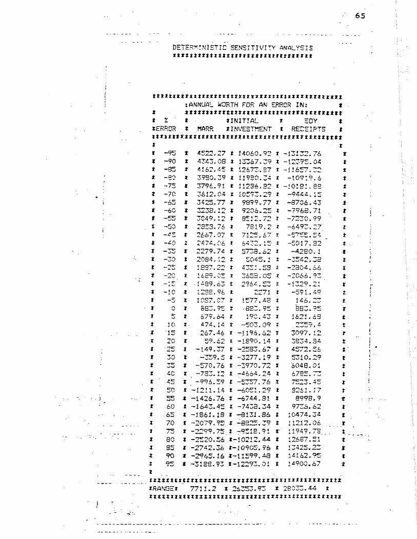
. ,
":,,".,
DE:TER~'!NIS7rC SENSITIVITY AN~L.YS!S Illltlllttlltillt •• ttfttt'ttttlltt
tllttltttttttttttrtt".tltllr'ltfrrrltllttlttl ,ANNUA~ kORTH FOR AN ERROR IN: f
t ~tttt.ttttttrtttltttftt.rttttt.ttttltt
t Z I .INITIAL t EOY t tERROR • !1ARR UN'JESTI':EI<T t RECEIPTS t tttlrt.tttttfttt •••• tlttrrrrrrr,rrtttt.rt'tttt t t
• f
• t
• t t t
•
-'15 -90 -85
-65 -60 -55
4~22;27 t 14060.92 f -13132.76 43~3.08 t 13367.39 t -!~395.0~ ~!6~.~S ~ 12673.27 t -!!657.~~
3990.39 t !198C.:~ t -!09:9.6 379t.91 t 11286.32 [ -!O!9:.2S ::'612.04 :: 3425 .. n t 3238.12 t '3C49.12 t
9899.77 I 9206 .. 25 t 8~!2,,7::; .t
-8706.43 -7968.71
t: -50 t 28:':3.76.t 7819.2 t -649~.:7 I
t t t t t t
-3"5 -30 -2;;
. •
-20. t
2t,b7.07 %
:47~.<:6 t :2279.7~ t
2084.:2 :;-1897.22 t
1~·e9.~:: : . 1 ~89 .. 63 t
7!:?::.67 !
643::.:5 t
5738 .. 62 t
::;045.1 %
43::: .. 59 t
3653.05 I
2.96L .. ::: :: ~ -10 t 1288.96 r :::71 :t
-:;
o
10 "15 20 25 30
% 10S7. C7: 15n. 4.8 t
.t 883 .. 9::!' . 8S::. 95 4:
-5/'2-::.S~
-5017.82 -4280.1
-3542 .. 32 -2804~66
-2066.93, _1"".,0 "':'<! . '-' ..... , " ........
J46.:3 853 .. 95
1621.69
3097.12 3834 .. 84 4572 .. 5t; 5310.29 6048.01
7::23 .. 45 92t1" 17
t
t r I
t I t t t t t t
t
I
t
t t
t
I
t t
60 65 70 75 80 95 90
t 679_6~ t 198.43 r .t. 474.14 t -503.09::: t 267.46 t -,1196.62 t
t 59~6.2 l -1890.14 r t -149.37 t -2583.67 f
t -359.5 f -3277.19 t t -570.76 J -3970,72 t f -783.12 t ~4664.24 t t -996.59 t -5:~7. 76 : t -12!1.14 t -6~!~29 t
t -1426.76 t -67~4.31 t t -1643.45 t -74~8.34 %
t -1861.19 I -8131.86 t t -2C79.95, , ~Be25.39 : t -~~9.75.~ ~,9~18.9! t" t -~20.56 t-l021:2.~ t t -2742.36 1-10905.?6 r t -2965.16 f-11599.AB t t -3les.93 1-12293~Ol t
8998.9 9736 .. 62
10474 .. 34 11212 .. 06 119~9.TS.
12687.~1
13425.2..3
t t .t
. . 1.:1162 .. 95 14 900.67
t
t%ttttlt~t%tttrttr:trrttttttr%tXtt%ittltzxxltt
IRANGEt 7711.2 l :6~5~,,~ x 28033.44 t
ltrttrttttrZtttfzttIIxtIXIII%lf:txlllllltt%IIt
t. t t t t
65

... _----EPROR IN LIFE TI~
EOY AN1\flJAL WORTH
1 -1000 2 -433 .. 96 ~
-' 109.53 4 526.01 '" . 883. 'i'5 ~
6 249";.03 7 3604.74 8 4405.19 9 5000 • .oil
".- •• -'-. -: '-.: > • .-
.. '; . . . -'~ .c.:- -.

Chapter 7.
SUMMARY.
In this study we have examined the techniques used to
evaluate capital investments.
For capital budgeting problems under certainty we
explore
average
five alternatives, namely net present value,payback,
return on book value, internal rate of return and
profitability index.
We also examined the use of mathematical programming
(linear programming, programming and goal
programming) for the
certainty. The aim of
integer
capital rationing problems under
combination of projects
these techniques is to find the
that will maximize shareholder's
wealth while not violating any budget constraint. We have
also examined Weingartner's
problem.
basic horizon model for this
For the capital
explored the use of
budgeting
sensitivity
urider uncertainty we
analysis/ break even
analysis, decision trees and simulation.
For the
included
capital rationing under uncertainty our
survey stochastic linear programming, chance-
constrained programming and quadratic programming. These
techniques will
maximize expected
determine the set of projects
shareholder's utility under
thaI. will
the complex
conditions of multi period uncertainty.
We tried to use and to develop computer programs that
can be applied for capital budgeting! rationing problem.
67

REFERENCENCES.
1. Brealey R., and Myers S.,: "Principles of Corporate
Finance", McGraw Hill, 1981.
2. Clark J.I., Hindelang T.H., and PritchardR.E.,: "Capital
Budgeting: PLanning and Control of Capital
Expenditures", Prentice Hall, 1979.
3. Levy H. , and Sarnat M. , : "Capital Investment and
Financial Decisions", Prentice Hall International, 1982.
4. Weingartner H.M.,: "Mathematical Programming and The
5 •
Analysis of Capital Budgeting Problems", Prentice Hall,
1963
3ernard R.H.,: "Mathematical Programming Models for
and Capital Budget:'ng: A
critique" Journal of
analysis, June 1966.
Survey.
financial
Generalization
-and Quant:'r:ative
6. Salazar R.C., and Sen S .K.,: "A .Simulation aodel of
Capital Budgeting Under
Science, December 1968.
7. 3ierman H .. , and Smidt S • , :
Decision", Macmillan Publishing
Certaintyl!,
"The Capital
Co Inc,1971.
8. Weston F.J., and Brigham E.F.,: "Manageri2.1
Holt Rinehart and Winston Inc, 1'972.
Management
Budgeting
Finance lf,
9. Lorie J.H., and Savage L.J. , : "Three Problems in
Rationing Capital", Journal of business, Oc:ober 1955.
68

69
10. Copeland- T.E., and Weston J.F.,: "Fi~ancial Theory and
Corporate Policy", Addison-Wesley,1979.
11. H~rtz D.B.,: 'fRisk Analysis in Capital Investment!',
Harvard Business review, January 1964.
12. Magee J.F.,: "How to Use Decision Trees in Capital
Investment", Harvard Business Review, September 1964.
13. Suarez J.A., and Tanchoco J.M.A.,: "Sensitivity Analysis
Aids in Evaluation of Investment", Industial Engineering
Magazine, March 1984.

APPENDIX
1 REM ---------2 REM DETERMINISTIC SENSITIVITY 3 REM -----------------4 HOME 5 6 7 8
TI$ = "SENSITIVITY ANALYSIS" T2$ = "FOR" T3$ = t'AN ECONOMIC EVALUATION" T4$ = 1I0FII
9 T5$ = "CAPITAL 10 VTAS 7: HTAS 11 FOR N = 1 TO 12 FOR I = 1 TO 13 FOR N = 1 TO 14 FOR I = 1 TO 15 FOR N = 1 TO 16 FOR I = 1 TO 17 FOR N = 1 TO 18 FOR I = 1 TO 19 FOR N = 1 TO 20 FOR I = 1 TO
PROJECTS" 10 LEN (TIS) :
50: NEXT I : LEN (T2$) :
50: NEXT ! : LEN (T3$) :
50: NEXT ' . .. LEN (T4$) :
50: . NEXT I : LEN (T5$) :
50: NEXT I :
PRINT NEXT N: PRINT NEXT N: PRINT NEXT N: PRINT NEXT N: PRINT NEXT N
MID$ (TU,N,I), PRINT : PRINT
MID$ (T2$~N.l) ; PRINT : PRINT
MID$ (T3$,N, 1): PRINT : PRINT
MID$ (T4$,N, 1); PRINT : PRINT
MID$ (T5$,N~ 1);
: HTAB 18
: HTA8 9
: HTAB 19
: HTA8 12
HOME pm:E
24 VTAB
: VTAB 2: HTAB 9: PRINT "ENTER THE "oLLOWING VALUES"
25 26 27 28 29 30
32
34,3 10: INPUT "INITIAL INVESTMENT $"jIN
VTAB 13: INPUT "UFE TIME (YEARS) "; YR VTAS 16: INPUT "MARR (PERCENT) " ; TE VTAB 19: I NPUT "SALVAGE VALUE "; SA HOME: HTAB 9: PRINT "SOY"; TAB ( 28); "RECEIPT" HTAB 9: PRINT "---"j TAB( 28);"----" DIM AW (200) , B (200) , MA C:OO) ,A (200) FOR G = 1 TO YR: HTAB :0 PRINT G:: HTAB 27: INPUT "$",A(G): NEXT G
33 POKE 34,0 34 HOME: VT-AB 12: HTAB 16: FLASH : PRINT "COMPUTING":: NORMAL 35 I = IE / 100 36 FOR R = - 99 TO 99: F = 1 + R / 100: Z = 0 37 FOR N = 1 TO YR:Z = Z ~ A(N) • (1 + I l PI ft ( - NI: NEXT N 38 00 = 1 + I l P: PW = -: N + Z + SAL t 00 ft ( - YR) 39 AW lR + 100 I = PW t « I I P * 00' YR) / (00 A YR - 1)
40 NEXT R 41 FOR NN = 1 TO 2: IF NN = 1 THE~J P = 1 - 99 / 100 42 IF NN = 2 THEN P = 1 ~ 99 / 100 43 Z = 0 44 FOR N = 1 TO YR:Z = Z - A(N) r P r (1 + I) ft ( - N): NEXT N 45 PW = - IN + Z + SAL r P r (1 + I) A ( - YRI 46 AA (NN) = PW r «I r (1 ~ 1) " YR I / « 1 + 1) A YR - 1l I : Z = 0 47 FOR N = 1 TO YR:Z = Z • A(N) r (1 ~ I) A ( - N): NEXT N 48 PW = - IN r P + SAL r (1 ~ I) ., ( - YR) + Z 49 WW iNN) = PW . * «l r (1 ~ 1) A YR) / ((1 ~ II A YR - 1)
50 NEXT NN
70

51 TU = AA(I}:TT = AA(2}:UT = WW(I}:ST = WW(2} 52 Z = O:L = 2 * YR - I:C = YR + I:XY = O:X = O:V = O:XSO = 0 53 FOR 5 = 1 TO YR 54 XY = XY + S • A(S}:X = X + S:Y = Y + A(S}:XSQ = XSO + SA: 55 NEXT S 56 B • (YR * XY - X • Y) I (YR * XSO - I ~ 2) 57 A = Y / YR - B • X / YR 59 DEF FN F(X) = A + 8 * X 59 DEF FN SAL (X) = (SAL - IN) / YR * X + IN 60 FOR N = C TO L;A(N} = FN F(N): NEXT N 61 FOR N = 1 TO L 62 Z = Z + A (N) tIl + II ~ I - N> 63 IF FN SALIN} < 0 THEN GOSUB 88: GOTO 67 64 PW = - IN + Z + FN SAL(N} • (1 + I) A ( - N) 65 MA IN} = PW * «(l • (1 + j) /, N} / «1 + 1) ~ N - 1})
66 B(N} = (100 • N) / YR - 100 67 NEXT N 68 HOME: VTAB 12: HTAB 17: FLASH: PRINT "SCAL:NG u
: NORMAL 69 K(I) = ABS (AW(l}):K(2) = ABS (AW(199»:K(3) = ASS (TTl 70 f~(4) = ASS (TU}:n5) = ABS (UT}:K(6) = ABS (ST) 71 K(7) = ABS (MA(I»:K(8) = ASS (MA(L - 1}):MAX = K(I) 72 FOR M = 2 TO 8 73 IF ~:: (M) > MAX THEN MAX = ~~·(M)
74 NEXT M:SC = INT (MAX / 5) 75 FOR U = 0 TO 900 STEP 100 76 77 78 79
IF 5C NEXT
L (1) = U (1) =
'. U AND SC , U
1000:L(2) 900o:uTZ)
80 FOR S = 1 TO 5 '
< = U +
= lE4: L(3) = 9E4:U(3}
100
= =
'iHEN SC
lE5:L(4) 9E5:U(4)
81 FOR U = LIS) TO U(S) STEP LIS)
= U ..- ,00: GOTO
= lEb:L(5) = lE7 = 9E6:U(5} = 9E7
36
82 IF SC ;. U AND SC < = IJ .;- LIS) THEN SC = U - US): GOTO 36 83 NEXT U 84 NEXT S 85 END 86 PRINT CHRS (4); "BLOAD CHAIN, A520" 87 CALL 520"GRAF1CA" 88 PW = - IN + Z:B(N) = 1100 • N) / YR - 100 89 MA (N) = PW • « I • (1 ... I) A N) I «! + [) A .~ - 1): REOJRN
71

90 91 92 93 94 95
REM REM REM DEF DEF HGR
GRAFICA
FN SeX) = FN G(X) =
HCOLOR= 6
INT «9 + 14 ; (5 f se - X) / SC) I NT (13.5 + 252 / 190 * (95 .. X»
96 HPLOT 140,0 TO 140,159: HPLOT 0,79 TO 279,79
+ .5)
97 FOR N = 14 TO 266 STEP 14: HPLOT N,79 TO N,77: NEXT N 98 FOR N = 9 TO 149 STEP 14: HPLOT 139,N TO 142,N: NEXT N 99 FOR N = 14 TO 210 STEP 14 100 FOR V = 2 TO 159 STEP 7 101 HPLOT N, V 102 NEXT V 103 NEXT N 104 FOR N = 224 TO 266 STEP 14 105 FOR V = 2 TO 114 STEP 7 106 HPLOT N, V
NEXT V NEXT N HCOLOR= 2 FOR N = - 99 TO 98:DE =-AW(N + 100) :RA-= AW(N + 101)
FN G(N), FN S(DE) TO FN G(N + 1), FN 5(RA) HPLOT NEXT N
107 108 109 110 111 112 113 114 115 116 117 118 119 120 121 1·":',/
HCDLOR= 5: HPLOT FN G ( - 99), .FN S WT) TO HCOLOR= 1: HPLOT FN G( - 99), FN S(TU) TO HCOlOR= 7:R = 2 t YR - 2
FN G(99), FN SCS,) FN G(99), FN S(TT)
124 125 126 127 128 129 130 131 132 133 134
FOR N = 1 TO R:SS = 8(N + l):SR = MA(N + 1) HPLOT FN G (B (N», FN S (MA eN» TO FN G (5S), FN S (SR) NEXT N HCOLOR= 6: HPLOT 58,84 TO 61,84 FOR N = 82 TO 84 STEP 2: HPlOT 63,N TO 66,N HPlOT 204, N TO 206. N: NEXT r, HPLOT 63,87 TO. 66,37: HPLOT 204,87 TO 206,87: HPlOT 64,83 HPLOT 204,83: HPLOT 66.85: HPLOT 206,85: HPLOT 66,86 riPlOT 206,86: HPlOT 70,82 TO 70,87: HPLOT 210,82 TO 210,87 HPLOT 74,82 TO 74,87: HPLOT 214,82 TO 214,87 HPLOT 72,82: HPLOT 212,82: HPLOT 72,87: HPLOT 212,87 HPLOT 66,96 TO 72,90: HPlOT 206,96 TO 212,90 FOR N = 90 TO 91: HPLOT 66,N: HPLOT 206,N HPLOT 64, N: HPLOT 204, N: NEXT N FOR N = 95 TO 96: HPLOT 74,N: HF'LOT 214.N
,0 252~ 128 ,0 266~ ''-'0 "'-' TO ~~.,
.... ..J ... ~ 1~~ ->-'
TO 264, 136: HP!..OT 268~ 132 TO TO 252,142
268, 136 136 137 138 139 140 141
~P!"OT 72. N: HPLOT 212, N: NEXT N HCDLOR= 7: HPLOT 224,128 ~COLOR= 6: HPLOT 266.125 HeGLOR:, 5: HPLOT 224~ 135 HCOLOR= 6: HPLOT 264. 132 HCOLOR= 2: HPLOT ~24,142 HCOLOR= 6: HPLOT 266.139 TO 266, 143: HPLOT 262~ 139 TO 262~143 f{PLOT 270,139 TO 270,143 HCOLOR= 1: HPlOT 224.149 TO 252,149: HCOLOR= 6 FOR N = 260 TO 272 STE.P 4: HPLOT N,146 TO N~ 150: NEXT N HOME : VTAB 21
142 PF;!NT TAB ( 2) "ANNUAL WORTH (Y1 VS % EST.ERROR (Xl" 143 PRINT TAB( 2) "AW SCALE: $";SC: TAB( 33) "!=YEAR8" 144 PRINT TAB( 2) "1I=INIT INVEST III=MARR I I Il=RECE:IPTS" 145 HTAB 8: PRINT "TYPE ANY KEY TO CONTINUE": GET K$ 146 HOME: VTAB 13: HTAB 15: FLASH: PRINT "PLEASE WAIT": NORMAL 147 PRINT CHR$ (4); "SlDAD CHAIN, A520" 148 CALL 520"GRAPH H
72

149 REM 150 REM GRAPH
151 152 153 154 155 156 157 158 159 160 161 162 163 164 165 166 167 168 169 170 171 172 173
REM HOME : PRINT PRINT PRINT PRINT PRINT FOR S PRINT PRINT PRINT PRINT PRINT PRINT FOR J
VTAB 22: HTAB 17: FLASH PRINT "PRINTING": NORMAL CHR$ (4);"PR#1" CHR$ (09) + "SON"
: PRINT : PRINT : PRINT : PRINT rAB( 24) "DETERMINISTIC SENSITIVITY ANALYSIS" TAB ( 24) "tnnnUufut**uutuunuuu"
= 1 TO 6: PRINT : NEXT S TAB( 25) "NET ANNUAL WORTH($) VS. I.-ERROR" TAB( 311"(X-AXIS) (Y-AXIS)"
PRINT : PRINT TAB ( 27)" I=VEARS CURVE" PRINT TAB ( 27)" II=INITIAL INVESTMENT CURVE" PRINT TAB ( 27)" I i I=MARR CURVE" PRINT TAB( 27) "IIII=EOY RECEIPT CURVE"
= 1 TO 10: PRINT : NEXT J CU = INT (AW (100) t 100 + .5) / 100
PRINT TAB ( 27) "ANNUAL WORTH (o7.ERROR): $", CU: PRINT PRINT TAB( 27)"ANNUAL WORTH SCALE '$";SC PRINT CHR$ (09) + "6"
PRINT CHR$ (4) "PRIIO": TEXT: HOME VTAB 12: HTAB 14 FLASH: PRINT "PLEASE WAIT": NORMAL PRINT CHR$ (4);"SLOAO CHAIN,A520" CALL 520"PRINTING"
73

174 REM 175 REM PRINTING 176 REM ---177 HOME VTAB 12: HTAB 16: FLASH PRINT "PRINTING": NORMAL 178 PRINT CHR$ (4)j"PR#I" 179 PRINT CHR$ (09) + "80N" 180 FOR Q = 1 TO 5: PRINT : NEXT Q 181 PRINT TAB( 24) "DETERMINISTIC SENSITIVITY ANALYSIS" 182 PRINT TAB ( 24)".*****: ••• **".".'*****' •••• *****" 183 FOR N = 1 TO 4: PRINT : NEXT N 184 HTAB 20: PRINT " •••••••••••••• *t.*.**.** ••••••• ************.**· 185 HTAB 20: PR I NT " : ANNUAL WORTH FOR AN ERROR IN: ... 186 HTAB 20: PRINT "t ***1.* •••• *** •••• ** •• ******.****.*** •• " 187 HTAB 20: PRINT ". 'l. t *INITIAL I EOY ." 188 HTAB 20: PRINT "tERROR t MARR *INVESTMENT I RECEIPTS ." 189 HTAB 20: PRINT "tnUUUUUUluu*un.UIUUUHUUUUI" 190 HTAB 20: PRINT "I I· 191 FOR MM = 5 TO 195 STEP 5 192 AW(MM) = INT (AW(MM) I 100 + .5) / 100: NEXT MM 193 K : TT - TU:S: 198:C = 100:E : ST - UT:J : 1 194 DEF FN EOY(X): INT «K / S * (X + 99) + TU) t C + .5) / C 195 DEF FN IN ( X ): I NT « E / S • (X +- 99) + un I C + • 5) / C 196 FOR N = - 95 TO 95 STEP 5 197 HTAB 20: PRINT "I "; SPC( 3 - LEN ( S,RS (N») ;N:" ."; 1 98 PR! NT SPC ( 9 - LEN ( STR$ ( AW (N + 100»»; AW (N + 1(0):" ." j 199 PRINT SPC( 9 - LEN (STR$ (FN IN(N»»: FN IN(N):" ."; 200 PRINT SPC ( 20 - LEN ( STR$ ( FN EOY (N) »); FN EOY (N);" 201 NEXT N 202 HTAB 20: PRINT 11*. 203 HTAB 20: PRINT " ••••••••••••• **** ••••• 11 ••• *1*.***** •••••••••• " 204 L : 2. t YR - 1: MA (U: I NT (MA (LJ * 100 + . 5) / 100 205 A ~ ABS· (AW (5) - AW (J 95» 206 C = ABS ( FN IN( - 95) - FN IN(95» 207 D = ABS ( FN EOY(95) - FN EOY( - 95» 208 D: INT CD f 100 ~ .5) / 100 209 210 211 212" 213 214 215 216 217 218 219 220 221 """ 4_~
225
HTAB 20:~ PRINT "tRANGD"; SPC ( 9 - LEN ( SIR$ (A»); A;" PRINT SPC( 9 - LEN ( STRS (C»);C;" PRINT SPC ( 9 - LEN ( STR$ (0») :D;"
FOR R = 1 TO 5: PRINT : NEXT R HTAB 31: PRINT "ERROR IN LIFE TIME" HTAB 31: PRINT II ---'
HTA8 30: PRINT "EOY ANNUAL WORTH" HTAB 30: PRINT "-
tlla ,
°FOR N : 1 TO L:MA(N) = HTAB 31: PRINT SPC( 2 -PRINT SPC ( 16 - LEN (
INT (MA(N) t 100 + 05) / 100 LEN ( STR$ (N») ;N:
STR$ (MA(N»»;MACN) NEXT N PRINT CHRs (4); "PR#O": HOME END
tu. ,
74