A Cellular Automata model for

Dictyostelium Discoideum

Katherine Goude, Simon O’Keefe

Advanced Computer Architecture Group

Department of Computer Science

University of York

August 24, 2005

Abstract

Cellular automata are abstract mathematical tools used for modelling

many different types of system. The aim of cellular automata is to create

complex behaviour through the interaction of many simple behaviours.

Dictyostelium discoideum is a slime mould with an unusual life cycle

which causes individual cells to come together and act as a multicellular

organism.

This report presents the modelling of Dictyostelium using a cellular

automaton, with the aim of reproducing its co-operative behaviour. We

discuss the issues involved when attempting to model a conservative sys-

tem such as a dictyostelium colony using cellular automata, and show that

it is possible to create sophisticated behaviour that mimics the behaviour

of the real organism using a small set of simple rules.

1

1 Introduction and Background

This technical report presents a model for generating the co-operative behaviourof the slime mould Dictyostelium Discoideum using a cellular automaton. Thebulk of the work described in this report was untertaken by Katherine Goudeas her third-year project for a BSc in Computer Science, during 2002-2003.The presentation of the material has been modified, but the content has notbeen substantially revised from that which was presented in her original projectreport.

The report is structured as follows. The first section gives a brief introductionto cellular automata and Dictyostelium Discoidium, and discusses the objectivesof the work. Section 2 discusses the implementation framework used to test thevarious automata. In section 3 the evolution of a cellular automaton is presented,the final version of which has behaviour similar to that of Dictyostelium in itsaggregation phase. Section 4 examines automata that attempt to reproducethe behaviour of Dictyostelium in its motile phase. The report ends with acomparison between the automata produced and other models of Dictyostelium,and gives some lines for further development of the automata.

1.1 Aims and objectives

The aim of this work is to model Dictyostelium Discoidium (Dicty) behaviourusing a cellular automaton as the method of representation. However, the focusis on testing the capabilities of cellular automata to simulate a biological organ-ism with co-operative behaviour rather than on furthering the understanding ofDicty behaviour.

A key point about previous models of Dicty is that they have been complex.The method used for modelling has been to attempt to mimic the way Dictybehaves in reality. They have been based on measured details of Dictyosteliumbehaviour and scientific principles, such as the equations of change in energy.The principal idea behind cellular automata is that complex behaviour can resultfrom very simple rules. To avoid simulating Dicty by imitating precise physicalprocesses, the approach taken here is to determine simple methods of recreatingDicty behaviour and test these more abstract ideas. The way the model worksdoes not have to be similar to the way Dicty works in reality. It is just theresultant behaviour which should aim to be similar to real life Dicty behaviour.The basic restrictions are:

1. All behaviour must be incorporated within a cellular automaton

2. The model should adhere to the formal definition of cellular automata

3. Simple rules should be used as far as possible

So the question which the work aims to answer is: Is it possible to model the

2

complex, co-operative behaviour of Dicty using a cellular automata model of

simple rules?

1.2 Cellular Automata

1.2.1 Definition of a Cellular Automaton

A cellular automaton is a regular lattice of identical “cells”, each of which canbe in any one of a finite number of states. Time advances in discrete stepsand at each step the state of every cell in the lattice is updated simultaneouslyaccording to a transition rule. This rule specifies the state a cell is to take atthe next time step as a function of its present state and the states of the cellswithin its neighbourhood.

The key features of a cellular automaton are the form of the lattice, the set ofstates a cell can be in, the neighbourhood of a cell and the transition function.

More formally,

let L be a regular lattice where the elements of L are cells

let S be a finite set of states where every cell c ∈ L has a state s ∈ S

let N be a finite set (of size n = |N |) of neighbourhood indices such that∀i ∈ N , ∀x ∈ L : (x + i) ∈ L

let F : Sn 7→ S be a local transition function

Then the 4-tuple (L,S,N ,F) is a cellular automaton.

Cellular automata have a huge capacity for variation. Aspects of cellular au-tomata which can be varied are:

The lattice The lattice can be of any size and shape. It can have any numberof dimensions although one and two dimensional cellular automata aremost common. The cells can also be various shapes as long as they canbe tessellated. There are various ways to treat cells on the boundary of alattice.

• In two dimensions, the lattice can be imagined as a torus with theedges wrapped around so that the top and bottom cells are connectedand the left and right cells are connected. This can be generalised tohigher dimensional lattices.

• The lattice can be reflected at the boundary.

• The cells on the boundary can be assigned a fixed value.

3

The set of states This could be anything from simple on or off (1 or 0) states,to a large set of structured variables such as arrays.

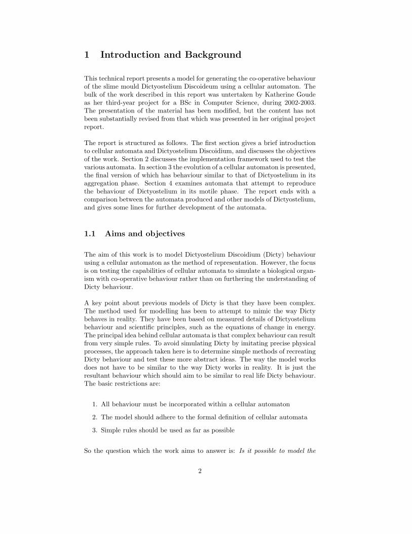
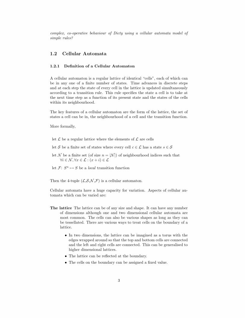
The neighbourhood A cell’s neighbourhood is the set of cells that it interactswith. In a grid these are normally the cells physically closest to the cellin question. Two particular 2-D neighbourhoods which are often used arethe Moore neighbourhood and the Von Neumann neighbourhood althoughthere are many possible variations.

Figure 1: The Moore neighbourhoodFigure 2: The Von Neumann neigh-bourhood

The transition function The transition function is the key part of a cellu-lar automaton. It determines the states of cells, and therefore the be-haviour of the cellular automaton. For every cellular automaton with Sstates and n cells in the neighbourhood, there are SS

n

possible transitionfunctions. Although in standard cellular automata, the transition func-tion is deterministic, stochastic cellular automata can be created usingnon-deterministic rules. These use a probability along with the states ofneighbouring cells to determine the new state of a cell.

Initial conditions The initial state of cells in the lattice is an important factorin the behaviour of a cellular automaton. Certain conditions may triggercomplex behaviour where others would not.

A typical mode of use of a cellular automaton is to observe each resultant stateafter the application of the transition rules and see the emerging behaviour.This is often used to create simulations. In this case the cellular automaton isrun in the same way as an animation. Each state following the application ofthe transition rules is displayed as a frame. The transition rules are repeatedlyapplied and the cellular automata can be seen evolving through subsequentstates.

The idea behind cellular automata is not to describe a complex system withcomplex equations, but to let the complexity emerge by interaction of simpleindividuals following simple rules. This can be seen in many biological systems,bird flocking for example. The phenomenon of complex behaviour arising frommany components with simple behaviour is common in natural systems.

4

1.2.2 Number conservation

Cellular automata consist of a fixed lattice, with each point on the lattice beingin some definite state. For some problems there is also a constraint on thenumber of lattice points that may be in a given state at any one time. Thisadditional constraint is referred to as number conservation, and is a necessaryconstraint if we wish to apply the CA model to problems such as modellingtraffic flow [11, 15] in which each vehicle is represented by a cell in a particularstate. It is clearly undesirable for the number of vehicles travelling on a sectionof road to vary, and therefore the rule governing the CA must ensure that thenumber of cells in the “vehicle” state does not vary. A theoretical analysisof this problem is presented by Boccara and Fuks [2], for a one-dimensionalfinite cellular automata with binary states. Durand et al. [5] take definitions offinite number-conservation and periodic number-conservation and prove theirequivalence to a class of number-conserving cellular automata in n dimensions.

In terms of our definitions above, we give the condition from [5] for a CA tobe NC. Consider a CA defined by the tuple (L,S,N ,F). The local transitionfunction F applied to a particular cell x, induces a global transition function Gcomposed of the simultaneous application of F to every cell in the lattice L (Gis defined only for for synchronous CA). The collection of states of the elementsof L is a configuration c ∈ C, where C is the set of possible configurations. Nowconsider a sequence of windows {Wk} on L, centred at the origin and of size2k +1. Denote by µk(c) the count of cells in the window Wk that are in a state

to be conserved, for a specific configuration c. Let M = lim supk→∞

µk(G(c))µk(c) . A

CA defined by (L,S,N ,F) is NC iff

1. G(0) = 0

2. ∀c ∈ C\{0}, M = 1

That is, in the limit the number of cells in the conserved state is the same beforeand after the application of the transition function whatever configuration theCA is in.

This report describes an implementation of a NC-CA that exhibits sophisticatedbehaviour analogous to that of a living organism, using a very small number ofrules.

1.2.3 Biological applications of CA

The biological applications of CA are varied. At one extreme are models thattake a non-local attribute of a particular biological system as their subject.Examples here include the modelling of “gene networks” within a particularbiological cell [4], in which each automaton cell represents the state of activationof a gene, and the rules governing interaction between automaton cells represent

5

the interactions between genes in the biological cell. This has been developedinto a model that may explain cell differentiation [16].

At the other extreme are models that take highly local attributes of a biologicalsystem and simulate the behaviour of the organism. Examples of this sort ofapproach are the CA models for Dictyostelium discoideum (see section 1.3) thatrepresent a single amoeba by a group of adjacent automaton cells. This is theapproach taken by Savill and Hogeweg [14], although their model is a hybridof a CA and partial differential equations. Strictly speaking this model doesnot conserve numbers, so the mass of the amoeba changes slightly as the modelruns.

Between between these two extremes lie models mapping amoebae onto singlelattice points on the CA. The localisation of the amoeba onto a single latticepoint makes number conservation absolutely essential, but also suggests a sim-pler approach to modelling the amoeba than in taken by for example Savill andHogeweg, or Palsson and Othmer [12].

1.3 Dictyostelium Discoideum

Dictyostelium discoideum is the name of a cellular slime mould which livesin forest soil. What is unusual about Dicty is that it has a social, altruisticnature. Under adverse conditions, Dicty amoebae1 come together to form amulti-cellular organism which then migrates until it finds an environment withmore suitable conditions. Some of the amoebae in this multi-cellular organismare destined to die once they have performed their purpose, the rest will even-tually disperse and continue as individuals once more. Due to its polymorphicbehaviour, Dicty is widely studied by biologists. It has been a useful source forstudying mechanisms such as chemotaxis (motion in response to a chemical),thermotaxis (motion in response to heat), phototaxis (motion in response tolight), and cellular sorting.

1.3.1 The Life-cycle of Dictyostelium

Under normal conditions, Dicty amoebae feed on bacteria and self-reproduce in-dependently. When food or water becomes scarce, some amoebae begin emittingregular pulses of a chemical attractant called cyclic adenosine monophosphate,or cAMP. These amoebae are called auto-cycling amoebae or pacesetters. Otheramoebae, when starving, become receptive to cAMP. When they detect cAMPthey respond to it by moving for a short time in the direction of its source andby emitting their own pulse of cAMP. This causes amoebae to form streamsall moving towards a centre point where the auto-cycling amoebae are emittingtheir periodic pulses. Eventually all amoebae from the area have aggregated

1To avoid confusion between Dictyostelium biological cells and the cells of cellular au-

tomata, this report will always refer to Dictyostelium cells as ‘amoebae’ and use ‘cell’ to mean

a component of a cellular automaton.

6

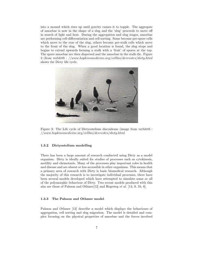
into a mound which rises up until gravity causes it to topple. The aggregateof amoebae is now in the shape of a slug and the ‘slug’ proceeds to move offin search of light and heat. During the aggregation and slug stages, amoebaeare performing cell-differentiation and cell-sorting. Some become pre-spore cellswhich move to the rear of the slug, others become pre-stalk cells which moveto the front of the slug. When a good location is found, the slug stops andbegins to extend upwards forming a stalk with a ‘fruit’ of spores at the top.The spore amoebae are then dispersed and the amoebae in the stalk die. Figure3 (from verbhttb : //www.hopkinsmedicine.org/cellbio/devreotes/dicty.htmlshows the Dicty life cycle.

Figure 3: The Life cycle of Dictyostelium discoideum (image from verbhttb ://www.hopkinsmedicine.org/cellbio/devreotes/dicty.html

1.3.2 Dictyostelium modelling

There has been a large amount of research conducted using Dicty as a modelorganism. Dicty is ideally suited for studies of processes such as cytokinesis,motility and chemotaxis. Many of the processes play important roles in healthand disease and are absent or less accessible in other organisms. This means thata primary area of research with Dicty is basic biomedical research. Althoughthe majority of this research is to investigate individual processes, there havebeen several models developed which have attempted to simulate some or allof the polymorphic behaviour of Dicty. Two recent models produced with thisaim are those of Palsson and Othmer[12] and Hogeweg et al. [14, 9, 10, 8].

1.3.3 The Palsson and Othmer model

Palsson and Othmer [12] describe a model which displays the behaviours ofaggregation, cell sorting and slug migration. The model is detailed and com-plex focusing on the physical properties of amoebae and the forces involved

7

throughout. These are features such as the changing shape and size of amoe-bae, chemotactic force, surface tension, cell stiffness, viscosity and adhesion.Each amoeba in the model is characterised by its location, orientation, its stateof stress and the forces it can exert. The cAMP pulses are modelled using areaction-diffusion equation.

The model operates by performing a repeated update procedure. At each updateall amoebae respond to any cAMP in the environment, change their orientationif necessary, calculate the net forces acting upon them, deform their shape andmove accordingly.

The results of the model show a good likeness to Dicty. However, the model isvery different from the one constructed here. The authors of that model are fromthe fields of mathematics and biology and their view point and purpose of themodel is very different from the present purpose. Their reason for creating themodel was that “many aspects of cell motion are poorly understood, includinghow individual cell behaviour produces the collective motion of cells observedwithin the mound and the slug.” Their aim was to create a biologically realisticmodel not only in the behaviour it produces but also in the way it works. Themodel was intended to aid understanding about how and why Dicty behaves asit does.

1.3.4 The Hogeweg et al. model

Other recent modelling activity of Dicty was begun in 1996 by Savill andHogeweg. This was extended over the following years to capture more of thebehaviour of Dicty. To date there have been four papers produced, describingthe model which now covers all main aspects of basic morphogenesis: aggrega-tion, slug migration, cell sorting, thermotaxis, phototaxis, and formation of thefruiting body [14, 9, 10, 8].

The model uses a technique developed by Glazier and Graner [6] where a cel-lular automaton is used to model amoebae movement. They use many cells tomake up each amoeba. Each cell contains a number showing which amoeba itis part of. Cells randomly copy the value of one of their neighbouring cells intothemselves and the probability of this happening is controlled by the energyreduction that the copying would cause. The energy is defined by two com-ponents; one is the discrepancy of the amoeba from its ideal volume and theother relates to the boundaries between cells. Each amoeba has an associatedtype and cells on the boundary of an amoeba have to take into account thesurface energy caused by the amoeba types of the neighbouring cells. The effectof this is that amoebae move around maintaining a fairly constant volume andsearching for lower energy levels. This causes amoeba to separate and sort intodifferent types with some types sticking together and others repelling. Thesemechanisms are useful for simulating the behaviour of Dicty so this method isused and extended by Hogeweg et al.

The model created is a hybrid cellular automaton and partial differential equa-

8

tion. The cellular automaton is used to represent the amoebae, the partialdifferential equation is used to model the cAMP. This model is simpler thanthat of Palsson and Othmer. Each cell in the cellular automaton represents asmall section of an amoeba. On average there are 60 cells per amoeba althoughthis varies during the running of the cellular automaton. At every update ofthe cellular automaton, a cell is chosen at random and one of its neighboursis copied into it with a probability dependant on the change in energy if thecopying were to occur. The equation for the change in energy takes into accountthe volume of the amoeba, its elasticity, the change in cAMP concentration, thebond energy between the amoeba and any neighbouring amoebae and also thebond energy between the amoeba and the medium of the environment. Thechange in cAMP concentration ensures that amoebae move towards areas ofhigher cAMP concentration, in other words the amoebae display chemotaxis.The bond energy is used for cellular adhesion. The differences in bond energiesbetween different types of amoebae means that cell sorting can occur. This isthe basic setup for the initial behaviour of aggregation and slug migration.

Extensions to the model have been made to simulate further behaviour. Ther-motaxis of the slug was produced by adjusting the cAMP threshold of someamoebae. The reasoning behind this being that heat is thought to cause amoe-bae to produce ammonia which causes changes in excitability. They show thatadding this difference in excitability of amoebae causes the cAMP waves tochange shape which causes the slug to turn in response to temperature gra-dients. Creating phototaxis of the slug was more complex. The model wasextended with a description of irradiation and refraction so that rays of lightcan be traced through the slug. An extra partial differential equation was addedto model ammonia, and the response of amoebae to cAMP became dependenton the ammonia concentration. Their results show that light does cause theslug to turn. The final extension to the model was for the culmination stage.Cell differentiation and rigidity were added, along with the ability for stalk cellsto produce an extracellular matrix. Differentiation is needed for amoebae tobecome stalk or spore cells. Rigidity is needed within the stalk. With theseadditions the model displays good results for the formation of the fruiting body.

As that model uses a cellular automaton and accomplishes all stages of Dic-tyostelium co-operative behaviour, the work presented here may seem redun-dant. However, that model has some drawbacks.

• The behaviour is not co-ordinated entirely by the cellular automaton. Apartial differential equation is also used for modelling of cAMP dynam-ics. Ideally the entire behaviour would be described purely by a cellularautomaton.

• One cell is updated at a time and this cell is chosen at random. That is,it is an asynchronous CA, rather than the synchronous CA reported here.

• The model is too complicated. To really test the property of cellularautomata to produce complex behaviour from simple rules, the modelshould avoid trying to imitate exact physical mechanisms.

9

2 Implementation Issues

The implemention of a cellular automaton to simulate the behaviour of Dictymay be broken down into a number of sub-tasks.

1. Create a representation of Dicty within the structure of a cellular automa-ton

2. Implement the cellular automaton structure in software

3. Add the transition rules to control the behaviour of the model

The key part of the model is the set of rules which reproduce the behaviour ofDicty. However, much of the implementation can be done before addressing thetransition rules. These implementation issues are described in this section.

2.1 The Representation

The first problem to be addressed is how Dicty can be represented within acellular automaton. Cellular automata are discrete and every cell is an identicalfinite state automaton. Encoding Dicty within the constraints of a cellular au-tomaton involves compromise as the cellular automaton is only an approximaterepresentation of the actual Dicty.

2.1.1 The Lattice

Decisions to be made about the lattice of the cellular automaton include: Howmany dimensions should the lattice have? What size should it be? What shapeshould the cells be? What neighbourhood will be used? How will the boundarybe dealt with?

A two-dimensional lattice is simpler to implement and understand than a three-dimensional lattice. Real-life Dicty exhibits three-dimensional behaviour. How-ever, Palsson and Othmer [12] use a two-dimensional model, based on work re-ported by Bonner [3]. Bonner had produced real life two-dimensional (one cellthick) Dicty slugs by trapping them between two glass plates. He showed thatthe behaviour of the slug was much the same as with normal three-dimensionalslugs. The process of aggregation is naturally two-dimensional. For these rea-sons the model uses a two-dimensional lattice.

Each cell is a square simply because this is easiest to implement and there is noreason to suppose that a different shape would be more appropriate.

The Moore neighbourhood is used as the local area of influence. This meansthat the new state of a cell depends on its previous state and the state of the

10

eight cells surrounding it. This seems most representative of the way an amoebais affected by its immediate environment.

Cells on the boundary of the lattice are dealt with by giving them a fixedvalue. Amoebae can then be prevented from moving into these ‘dummy’ cellsto simulate hitting the edge of a container. The cAMP simply disappears overthe edge of the grid.

The question of the size of the lattice can not be answered until the size of cellsrelative to amoebae is decided. A representation using several amoebae per cellwill require a very different sized lattice to a representation using several cellsper amoeba.

2.1.2 The Cells

Decisions to be made about the cells of the cellular automaton include: Whatshould the states of the cells be? What information do they store? What is theinitial state?

The cellular automata model of Hogeweg et al uses many cells to represent asingle amoeba. A simpler approach is to allow a single amoeba to occupy acell. Then the state of that cell represents the entire state of the amoeba. Adrawback with this is that it constrains the ability of amoebae to slide over andpast each other. If an amoeba is surrounded by eight other amoebae then it iseffectively trapped. One way to avoid this is to allow multiple amoeba to occupyeach cell. By allowing up to four amoebae to occupy a cell without specifyinga sub-cellular location, amoebae can move between cells without being blocked.It is also more natural in that it can simulate amoebae sliding over or past eachother. This can be understood by thinking about an amoeba wishing to moveinto the cell to its north. If there are two amoebae in the northern cell, theymight both be in the side of the cell towards the amoebae wishing to move,in which case it would be blocked. However, since the cells do not designatea particular position within the cell for an amoeba to be, then the movingamoeba will be allowed into the northern cell as if it has slid over the two in itspath. An amoeba is trapped only if it is surrounded by 32 other amoebae. Theother key reason for using four amoebae per cell is to simplify the movement ofamoebae following a cAMP pulse. Amoebae move the distance of two amoebaediameters during a response to a single cAMP pulse. With four amoebae percell this movement equates to moving from one cell into a neighbouring cell.

The state of the cells within the cellular automaton should store all necessaryinformation about their contents. In the case of amoebae occupying the cell,the key piece of information to store would be the current state of each amoeba.Some amoebae emit pulses of cAMP periodically. All other amoebae may be in-active and receptive to cAMP, responding to cAMP or recovering after a cAMPresponse. These four states are referred to as pacesetter, ready, excited andresting respectively. Since each cell can contain up to four amoebae, the stateof a cell contains the states of four independent amoebae. The state ‘empty’

11

can also be thought of as a possible state of an amoeba and just represents anempty space.

Unlike the model of Hogeweg et al, this implementation should encompass themodelling of cAMP within the cellular automaton. This means that any nec-essary variables to indicate cAMP level within the cell and to control cAMPmovement between cells should all be stored as part of the state of a cell.

The state of a cell is also used to store other information required for updating,such as a timer variable to control the regular cAMP pulses emitted by pace-setter amoebae. This increases the complexity of state of a cell. However mostof this can be internal to the algorithm. The only aspects which need to beobservable are those that a viewer needs to judge the resulting behaviour. Theobservables are thus the state of each amoeba and the level of cAMP in eachcell.

The initial state of the cells should be a random distribution of amoebae acrossthe grid. The cAMP value at all cells should initially be zero. By adding afew pacesetter amoebae to the centre of the grid, this simulates the start ofmorphogenesis, when amoebae begin to starve.

2.2 The Simulation Framework

2.2.1 Programming Environment

The simulation is implemented as a Java Applet using JBuilder, due to theease of using Java to create graphical user interfaces. Java has good librariesfor building GUIs and is easy to use to program responses to events at theinterface.

2.2.2 The Interface

The interface is implemented with the lattice of the cellular automaton displayedon the right and a control panel to the left. See figure 4 for a screen shot of theinterface.

2.2.3 The Display

The cellular automaton has a two-dimensional lattice composed of square cellseach containing up to four amoebae. The number of Dicty amoebae aggregatingtogether is typically in the region of 10,000 – 100,000. The population densityof amoebae before aggregation is not clear from the literature so this becomesa factor to determine experimentally during testing. However, to determine thesize for the grid of the cellular automaton, an initial estimate of population

12

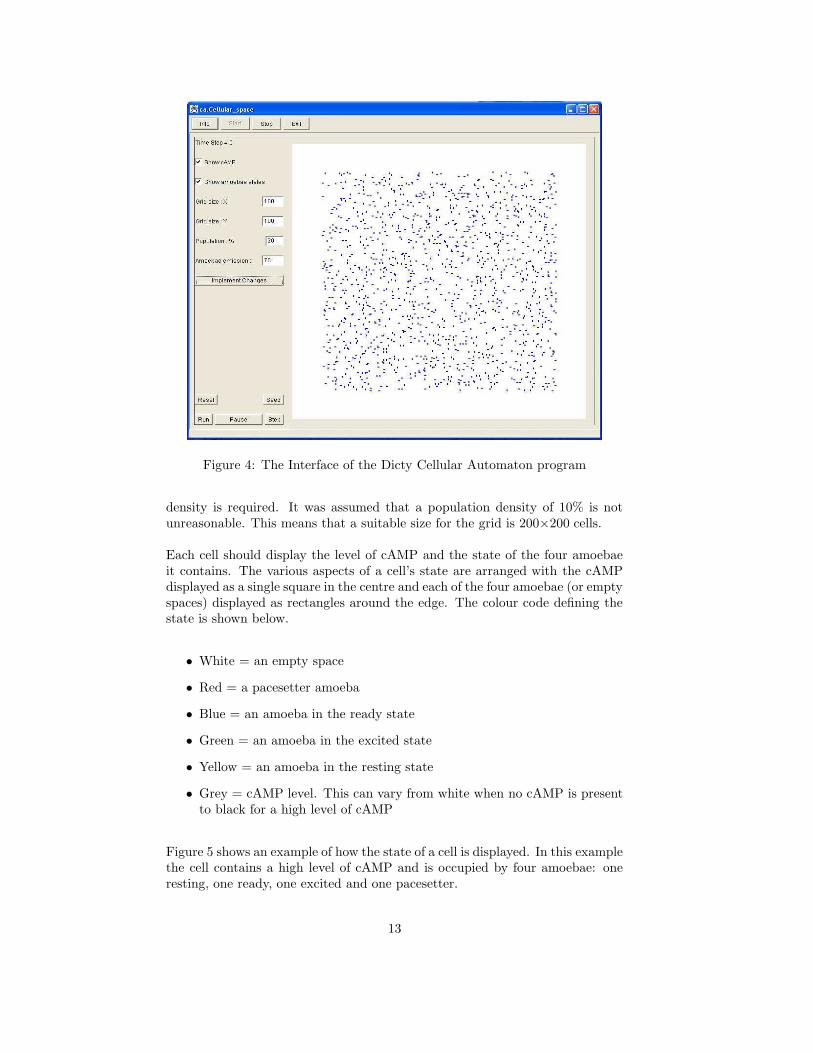
Figure 4: The Interface of the Dicty Cellular Automaton program

density is required. It was assumed that a population density of 10% is notunreasonable. This means that a suitable size for the grid is 200×200 cells.

Each cell should display the level of cAMP and the state of the four amoebaeit contains. The various aspects of a cell’s state are arranged with the cAMPdisplayed as a single square in the centre and each of the four amoebae (or emptyspaces) displayed as rectangles around the edge. The colour code defining thestate is shown below.

• White = an empty space

• Red = a pacesetter amoeba

• Blue = an amoeba in the ready state

• Green = an amoeba in the excited state

• Yellow = an amoeba in the resting state

• Grey = cAMP level. This can vary from white when no cAMP is presentto black for a high level of cAMP

Figure 5 shows an example of how the state of a cell is displayed. In this examplethe cell contains a high level of cAMP and is occupied by four amoebae: oneresting, one ready, one excited and one pacesetter.

13

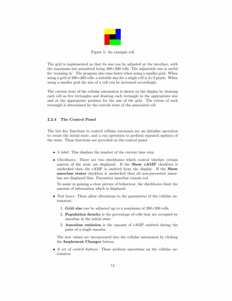
Figure 5: An example cell

The grid is implemented so that its size can be adjusted at the interface, withthe maximum size permitted being 200×200 cells. The adjustable size is usefulfor ‘zooming in’. The program also runs faster when using a smaller grid. Whenusing a grid of 200×200 cells, a suitable size for a single cell is 3×3 pixels. Whenusing a smaller grid the size of a cell can be increased accordingly.

The current state of the cellular automaton is shown on the display by drawingeach cell as five rectangles and drawing each rectangle in the appropriate sizeand at the appropriate position for the size of the grid. The colour of eachrectangle is determined by the current state of the associated cell.

2.2.4 The Control Panel

The two key functions to control cellular automata are an initialise operationto create the initial state, and a run operation to perform repeated updates ofthe state. These functions are provided on the control panel.

• A label: This displays the number of the current time step

• Checkboxes: There are two checkboxes which control whether certainaspects of the state are displayed. If the Show cAMP checkbox isunchecked then the cAMP is omitted from the display. If the Showamoebae states checkbox is unchecked then all non-pacesetter amoe-bae are displayed blue. Pacesetter amoebae remain red.

To assist in gaining a clear picture of behaviour, the checkboxes limit theamount of information which is displayed.

• Text boxes: These allow alterations to the parameters of the cellular au-tomaton:

1. Grid size can be adjusted up to a maximum of 200×200 cells

2. Population density is the percentage of cells that are occupied byamoebae in the initial state

3. Amoebae emission is the amount of cAMP emitted during thepulse of a single amoeba

The new values are incorporated into the cellular automaton by clickingthe Implement Changes button.

• A set of control buttons: These perform operations on the cellular au-tomaton

14

1. Reset initialises the cellular automaton and causes the initial stateto be displayed

2. Seed adds pacesetter amoebae to the cellular automaton so thatcAMP is produced and co-operative behaviour can begin

3. Step performs a single update of the cellular automaton and displaysthe new state

4. Run performs updates repeatedly and displays each resultant stateas it progresses

5. Pause stops the running procedure and leaves the most recent statedisplayed

2.2.5 The Update Procedure

The update procedure of a cellular automaton is the process carried out tosimulate one time step. It creates a mapping from one set of states to anotherset produced by applying the transition rules to each cell. The update procedureof cellular automata is theoretically a parallel operation, as the updating shouldoccur at every cell simultaneously. However, this can be easily implementedusing normal sequential coding simulating a parallel update. The only drawbackis that the time taken to update the entire lattice is proportional to the numberof cells. The sequential update procedure uses two separate representations ofthe cellular automaton grid. One is used to store the current state, the otherto store the new state. The update can be carried out one cell at a time wherethe state is always read from the current grid and written to the new grid. Onceall cells have been updated, the contents of the new grid are copied into thecurrent grid. This is one time step.

2.2.6 Program structure

The classes used to structure the code are discussed in Appendix A.

15

3 Aggregation

In this section, the behaviour of Dictyostelium is considered, and sets of cellularautomaton transition rules are produced and refined.

3.1 Dicty Aggregation Behaviour

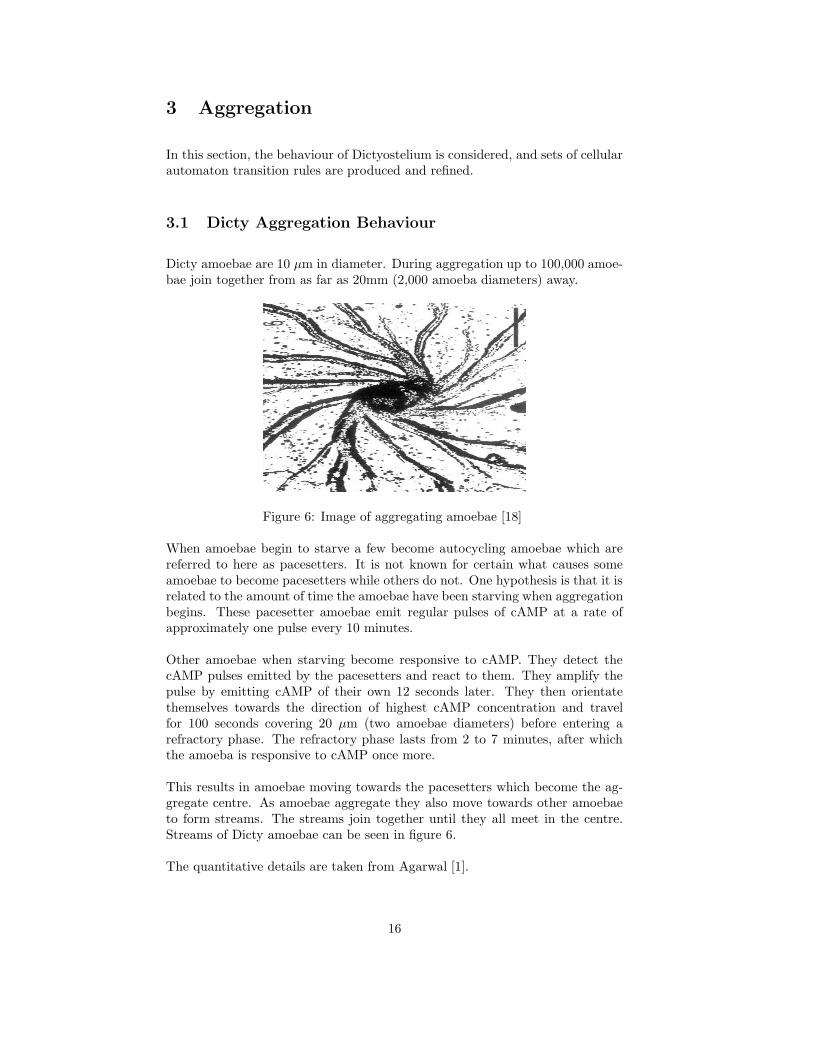
Dicty amoebae are 10 µm in diameter. During aggregation up to 100,000 amoe-bae join together from as far as 20mm (2,000 amoeba diameters) away.

Figure 6: Image of aggregating amoebae [18]

When amoebae begin to starve a few become autocycling amoebae which arereferred to here as pacesetters. It is not known for certain what causes someamoebae to become pacesetters while others do not. One hypothesis is that it isrelated to the amount of time the amoebae have been starving when aggregationbegins. These pacesetter amoebae emit regular pulses of cAMP at a rate ofapproximately one pulse every 10 minutes.

Other amoebae when starving become responsive to cAMP. They detect thecAMP pulses emitted by the pacesetters and react to them. They amplify thepulse by emitting cAMP of their own 12 seconds later. They then orientatethemselves towards the direction of highest cAMP concentration and travelfor 100 seconds covering 20 µm (two amoebae diameters) before entering arefractory phase. The refractory phase lasts from 2 to 7 minutes, after whichthe amoeba is responsive to cAMP once more.

This results in amoebae moving towards the pacesetters which become the ag-gregate centre. As amoebae aggregate they also move towards other amoebaeto form streams. The streams join together until they all meet in the centre.Streams of Dicty amoebae can be seen in figure 6.

The quantitative details are taken from Agarwal [1].

16

3.2 Design of Transition Rules

Dicty behaviour is determined by two separate factors: the cAMP, and theamoebae themselves. Updating the states of amoebae requires reference to thesurrounding cAMP and updating the cAMP value of a cell requires reference toany emitting amoebae. Each factor affects the other but both can be describedindependently. The cellular automaton update function calls two separate op-erations: one to update the cAMP aspects of state, and the other to update theamoebae aspects of state.

3.2.1 Amoeba Behaviour

The transitions between the different states of amoebae are clearly defined.The state of pacesetter amoebae is fixed. Their only behaviour is the periodicemission of cAMP. All other amoebae become responsive to cAMP when theybegin starving and this is the ready state. When a ready amoeba detects cAMP,it becomes excited. Once an excited amoeba has moved towards the source ofthe cAMP, it then changes to a resting state. After a certain period of timea resting amoeba returns to the ready state. The assumption is made thatamoebae will only move when responding to cAMP.

Ignoring timing constraints, these state transitions of amoebae can be modelledby the following rules:

1. PACESETTER → PACESETTER

2. READY → EXCITED if cAMP is detected

3. READY → READY otherwise

4. EXCITED → RESTING once the amoeba has moved

5. EXCITED → EXCITED until then

6. RESTING → READY

There are two aspects of cAMP involvement which need to be addressed: Howcan amoebae detect cAMP and determine when to change state from ready toexcited? How can amoebae determine the direction of the cAMP origin?

When in the ready state, amoebae should be monitoring the surrounding cAMPlevel. In reality Dicty amoebae do this by reaching out cAMP receptors inseveral directions to detect cAMP and to then know which direction it originatedfrom.

The simplest way to decide when to change state from ready to excited is byapplying a threshold to the cAMP value of the cell. If the value exceeds thethreshold then the amoeba changes state. Otherwise it remains in the ready

17

state. A suitable level for this excitation threshold can be determined duringtesting.

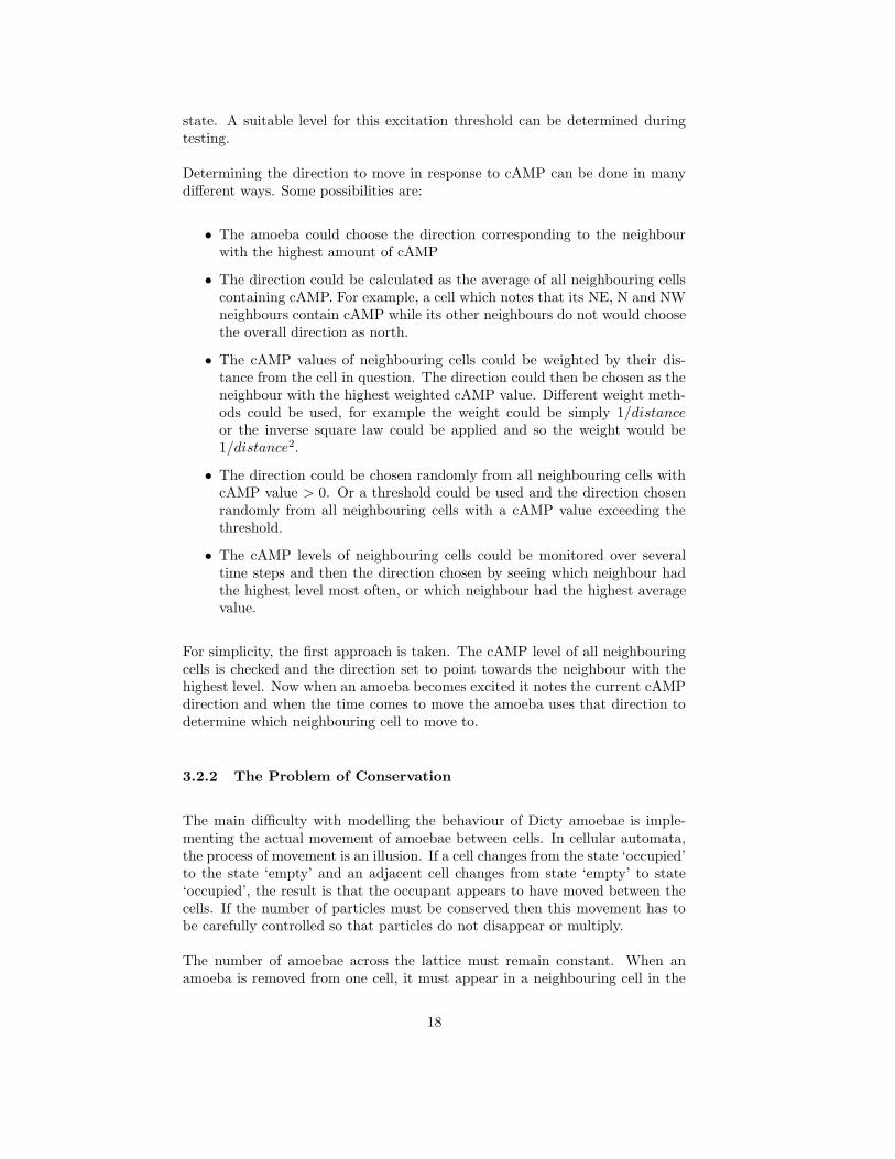
Determining the direction to move in response to cAMP can be done in manydifferent ways. Some possibilities are:

• The amoeba could choose the direction corresponding to the neighbourwith the highest amount of cAMP

• The direction could be calculated as the average of all neighbouring cellscontaining cAMP. For example, a cell which notes that its NE, N and NWneighbours contain cAMP while its other neighbours do not would choosethe overall direction as north.

• The cAMP values of neighbouring cells could be weighted by their dis-tance from the cell in question. The direction could then be chosen as theneighbour with the highest weighted cAMP value. Different weight meth-ods could be used, for example the weight could be simply 1/distanceor the inverse square law could be applied and so the weight would be1/distance2.

• The direction could be chosen randomly from all neighbouring cells withcAMP value > 0. Or a threshold could be used and the direction chosenrandomly from all neighbouring cells with a cAMP value exceeding thethreshold.

• The cAMP levels of neighbouring cells could be monitored over severaltime steps and then the direction chosen by seeing which neighbour hadthe highest level most often, or which neighbour had the highest averagevalue.

For simplicity, the first approach is taken. The cAMP level of all neighbouringcells is checked and the direction set to point towards the neighbour with thehighest level. Now when an amoeba becomes excited it notes the current cAMPdirection and when the time comes to move the amoeba uses that direction todetermine which neighbouring cell to move to.

3.2.2 The Problem of Conservation

The main difficulty with modelling the behaviour of Dicty amoebae is imple-menting the actual movement of amoebae between cells. In cellular automata,the process of movement is an illusion. If a cell changes from the state ‘occupied’to the state ‘empty’ and an adjacent cell changes from state ‘empty’ to state‘occupied’, the result is that the occupant appears to have moved between thecells. If the number of particles must be conserved then this movement has tobe carefully controlled so that particles do not disappear or multiply.

The number of amoebae across the lattice must remain constant. When anamoeba is removed from one cell, it must appear in a neighbouring cell in the

18

same time step. This is not a simple task when amoebae are not objects to bemoved around but are merely aspects of a cell’s state.

When an amoeba wants to move, it knows the direction it wants to move in andtherefore which neighbouring cell that corresponds to. It needs to check thatthe cell has an empty space in the current time step and that no other amoebaehas yet taken it ready for the next time step. Since the model should simulatea parallel update operation, this checking is not possible.

If a move was to occur, the cell currently containing the amoeba would have tochange the amoeba state to the empty state. At the same time, the cell withthe empty space must somehow know to assign the amoeba to the space.

Imagine a cell, C, containing two amoebae and two empty spaces. At time stept there are three amoebae from surrounding cells that wish to move into cell Cin time step t + 1. How can collisions be avoided in the next time step? Howwill the amoebae desiring to move to cell C know whether they are permitted tooccupy a space in C or not? How will cell C know which neighbouring amoebaeit should copy into its empty spaces? Should amoebae be allowed to push eachother out of the way, and if so how can this be co-ordinated?

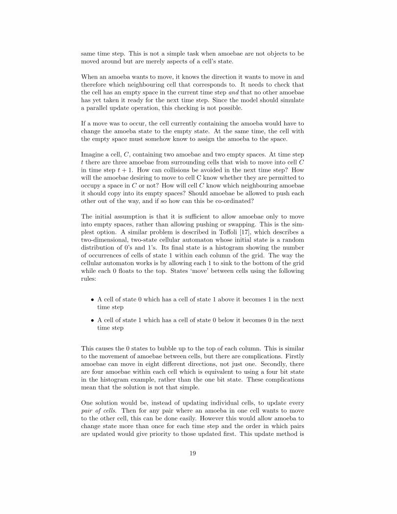
The initial assumption is that it is sufficient to allow amoebae only to moveinto empty spaces, rather than allowing pushing or swapping. This is the sim-plest option. A similar problem is described in Toffoli [17], which describes atwo-dimensional, two-state cellular automaton whose initial state is a randomdistribution of 0’s and 1’s. Its final state is a histogram showing the numberof occurrences of cells of state 1 within each column of the grid. The way thecellular automaton works is by allowing each 1 to sink to the bottom of the gridwhile each 0 floats to the top. States ‘move’ between cells using the followingrules:

• A cell of state 0 which has a cell of state 1 above it becomes 1 in the nexttime step

• A cell of state 1 which has a cell of state 0 below it becomes 0 in the nexttime step

This causes the 0 states to bubble up to the top of each column. This is similarto the movement of amoebae between cells, but there are complications. Firstlyamoebae can move in eight different directions, not just one. Secondly, thereare four amoebae within each cell which is equivalent to using a four bit statein the histogram example, rather than the one bit state. These complicationsmean that the solution is not that simple.

One solution would be, instead of updating individual cells, to update everypair of cells. Then for any pair where an amoeba in one cell wants to moveto the other cell, this can be done easily. However this would allow amoeba tochange state more than once for each time step and the order in which pairsare updated would give priority to those updated first. This update method is

19

also contrary to the definition of cellular automata as it no longer simulates aparallel operation.

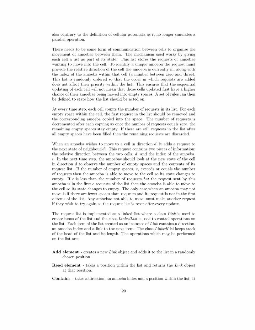
There needs to be some form of communication between cells to organise themovement of amoebae between them. The mechanism used works by givingeach cell a list as part of its state. This list stores the requests of amoebaewanting to move into the cell. To identify a unique amoeba the request mustprovide the relative direction of the cell the amoeba is currently in, along withthe index of the amoeba within that cell (a number between zero and three).This list is randomly ordered so that the order in which requests are addeddoes not affect their priority within the list. This ensures that the sequentialupdating of each cell will not mean that those cells updated first have a higherchance of their amoebae being moved into empty spaces. A set of rules can thenbe defined to state how the list should be acted on.

At every time step, each cell counts the number of requests in its list. For eachempty space within the cell, the first request in the list should be removed andthe corresponding amoeba copied into the space. The number of requests isdecremented after each copying so once the number of requests equals zero, theremaining empty spaces stay empty. If there are still requests in the list afterall empty spaces have been filled then the remaining requests are discarded.

When an amoeba wishes to move to a cell in direction d, it adds a request tothe next state of neighbour[d]. This request contains two pieces of information;the relative direction between the two cells, d, and the index of the amoeba,i. In the next time step, the amoebae should look at the new state of the cellin direction d to observe the number of empty spaces and the contents of itsrequest list. If the number of empty spaces, e, exceeds or equals the numberof requests then the amoeba is able to move to the cell so its state changes toempty. If e is less than the number of requests but the request sent by thisamoeba is in the first e requests of the list then the amoeba is able to move tothe cell so its state changes to empty. The only case when an amoeba may notmove is if there are fewer spaces than requests and its request is not in the firste items of the list. Any amoebae not able to move must make another requestif they wish to try again as the request list is reset after every update.

The request list is implemented as a linked list where a class Link is used tocreate items of the list and the class LinkedList is used to control operations onthe list. Each item of the list created as an instance of Link contains a direction,an amoeba index and a link to the next item. The class LinkedList keeps trackof the head of the list and its length. The operations which may be performedon the list are:

Add element - creates a new Link object and adds it to the list in a randomlychosen position.

Read element - takes a position within the list and returns the Link objectat that position.

Contains - takes a direction, an amoeba index and a position within the list. It

20

then returns true if a link matching the direction and index occurs beforethe specified position in the list. Otherwise false is returned.

This list enables the co-ordination of amoeba movement.

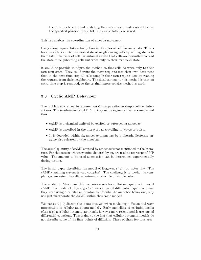
Using these request lists actually breaks the rules of cellular automata. This isbecause cells write to the next state of neighbouring cells by adding items totheir lists. The rules of cellular automata state that cells are permitted to readthe state of neighbouring cells but write only to their own next state.

It would be possible to adjust the method so that cells do write only to theirown next state. They could write the move requests into their own next statethen in the next time step all cells compile their own request lists by readingthe requests from their neighbours. The disadvantage to this method is that anextra time step is required, so the original, more concise method is used.

3.3 Cyclic AMP Behaviour

The problem now is how to represent cAMP propagation as simple cell-cell inter-actions. The involvement of cAMP in Dicty morphogenesis may be summarisedthus:

• cAMP is a chemical emitted by excited or autocycling amoebae.

• cAMP is described in the literature as travelling in waves or pulses.

• It is degraded within six amoebae diameters by a phosphodiesterase en-zyme also released by the amoebae.

The actual quantity of cAMP emitted by amoebae is not mentioned in the litera-ture. For this reason arbitrary units, denoted by au, are used to represent cAMPvalue. The amount to be used as emission can be determined experimentallyduring testing.

The initial paper describing the model of Hogeweg et al. [14] notes that “ThecAMP signalling system is very complex”. The challenge is to model the com-plex system using the cellular automata principle of simple rules.

The model of Palsson and Othmer uses a reaction-diffusion equation to modelcAMP. The model of Hogeweg et al. uses a partial differential equation. Sincethey were using a cellular automaton to describe the amoebae behaviour, whynot just incorporate the cAMP within that same model?

Weimar et al [19] discuss the issues involved when modelling diffusion and wavepropagation in cellular automata models. Early modelling of excitable mediaoften used a cellular automata approach, however more recent models use partialdifferential equations. This is due to the fact that cellular automata models donot describe some of the finer points of diffusion. Three of these features are:

21

Curvature Curved waves travel at different speeds

Dispersion The speed of waves depends upon the state of the medium in frontof the wave

Isotropy The speed of waves should be the same in all directions

The curvature problem can be solved by using larger neighbourhoods but thisincreases complexity. Dispersion can be modelled by taking into account therecovery of a cell. Solving isotropy requires a large amount of computation andthis is inefficient. The paper describes discrete approximations to the diffusionequation which can then be modelled using a cellular automaton. The solutionspresented are not useful to the present context, however. They are a way ofmodelling chemical diffusion in an accurate but complex manner. The crite-ria for this task of modelling Dicty require simple rules and an approximatemodel for cAMP propagation should be adequate in this case. Concepts suchas curvature, dispersion and isotropy are not important in this context.

Toffoli [17] describes a method of creating pulses which expand and overlap likeripples in water. These pulses are created in a cellular automaton with threestates which could be named as ready, pulsing and refractory. The transitionsrules are very simple:

• ready → pulsing if any neighbour is pulsing

• ready → ready otherwise

• pulsing → refractory

• refractory → ready

If some cells are set to pulse in the initial state then when the cellular automa-ton begins running, pulses expand outwards from those points. Where theycollide, they join together to make one large pulse which keeps expanding. Therefractory state ensures that pulses always travel outward.

Since cAMP waves are always described as moving as pulses, an adaption ofthis idea has been used in the model. The pulses have to be degraded so thisrequires describing the pulse by an amount rather than a present/absent state.A boolean variable is used to show whether a cell is in the refractory state ornot. The cAMP amount of a cell will depend upon the amounts in neighbouringcells. The amount of cAMP is set to the highest of the values of neighbouringcells with a degradation constant subtracted. If there are any emitting amoebaewithin the cell then these emissions need to be added to the amount.

One key flaw with this pulse method is that when used on a square grid, thepulses will also be square. This can be helped slightly by using a higher degrada-tion when cAMP passes from a cell to a diagonal neighbour since this distance isgreater. Diagonal degradation will be equal to adjacent degradation multipliedby

√2.

22

The amount of cAMP that amoebae emit and the amount of degradation willdetermine how far the pulses travel. These values can be experimented withduring the testing stage. The amount of cAMP is measured in arbitrary units(au) so the units of emission and degradation will be au and au per time step(ts) respectively.

3.3.1 Design Methodology

“Science has little use for models that slavishly obey all of ourwishes. We want to get out of our models more than we have putin. A reasonable way to start is to put in as little as possible.”— Toffoli [17].

The method used to build the model is to start with some initial, simple ideasand then create an implementation to experiment with those ideas. The programframework described in Section 2 means that implementing these ideas justrequires writing the body of the ‘update cAMP’ and ‘update amoebae’ functions.The results gained and conclusions made are then fed back into the design tocreate changes and improvements to the model. The design-implementation-conclusion cycle is an iterative process, and the different versions of the modelalong with the results and conclusions of each are discussed in the followingsections.

3.4 Aggregation Version 1

The initial ideas described above are implemented in this first model. Theamoebae behaviour is modelled by simple state transitions and the cAMP isdescribed by rules which produce pulses.

3.4.1 Results

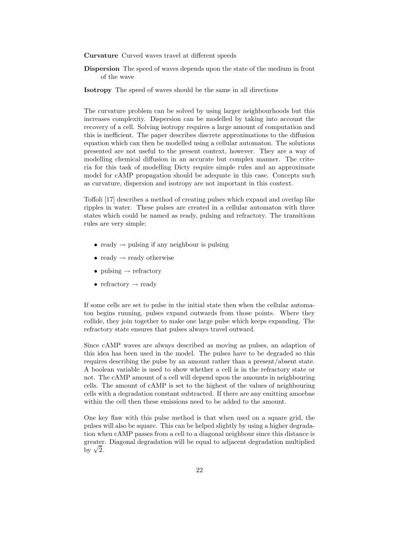
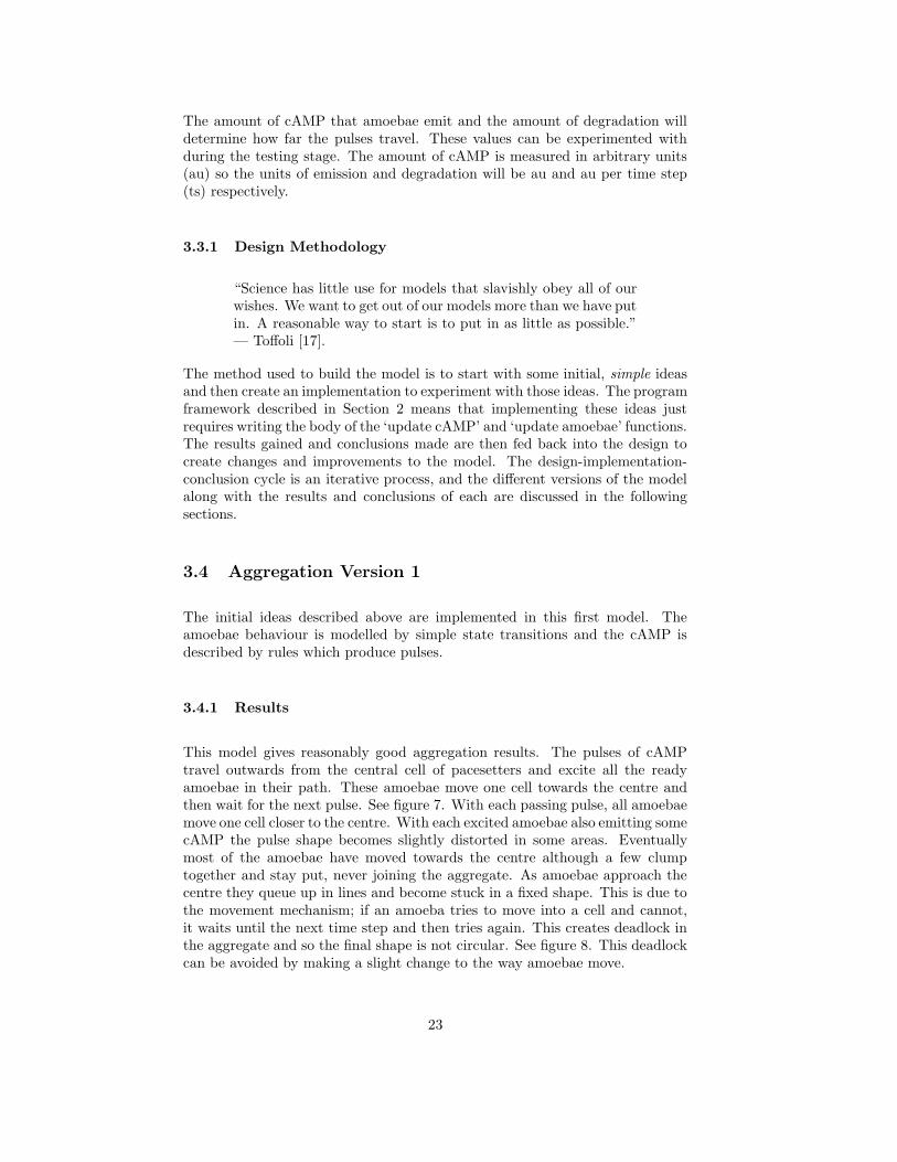
This model gives reasonably good aggregation results. The pulses of cAMPtravel outwards from the central cell of pacesetters and excite all the readyamoebae in their path. These amoebae move one cell towards the centre andthen wait for the next pulse. See figure 7. With each passing pulse, all amoebaemove one cell closer to the centre. With each excited amoebae also emitting somecAMP the pulse shape becomes slightly distorted in some areas. Eventuallymost of the amoebae have moved towards the centre although a few clumptogether and stay put, never joining the aggregate. As amoebae approach thecentre they queue up in lines and become stuck in a fixed shape. This is due tothe movement mechanism; if an amoeba tries to move into a cell and cannot,it waits until the next time step and then tries again. This creates deadlock inthe aggregate and so the final shape is not circular. See figure 8. This deadlockcan be avoided by making a slight change to the way amoebae move.

23

Figure 7: V1. Initial Aggregation Behaviour

If an amoeba makes a request to move into a neighbouring cell C and on thenext time step discovers that its request failed then its response should be torandomly choose another neighbouring cell either to the left or right of cell C.It should then make its next request to the new cell. This can continue untila request is successful. This introduces a random factor into the model andmakes it a stochastic cellular automaton. It means that amoebae can movearound other amoebae in their path. The result of this change is that the finalaggregate is now more circular. When amoebae become blocked they find adifferent route to the centre. This change also means that amoebae movementnever stops; while the pacesetters are still emitting cAMP and exciting theamoebae aggregate then the amoebae keep on trying to move. This is not aproblem since any amoebae moving away from the aggregate will always moveback again the next time they move. Another change is that the pulse shapebecomes more irregular in the later stages of aggregation. See figure 9.

Figure 8: V1. Final, fixed aggregateFigure 9: V1. Aggregate with randommotion

Experimentation with different values for cAMP degradation, amoebae emissionand population density shows the following. This model works only when using a

24

low population density, in the region of 5%. With a higher density the amoebaeform several loose clumps near the centre but remain quite scattered. Theideal degradation and emission values for this model are 7 au/ts and 150 aurespectively. Recall that emission and degradation are measured in arbitraryunits of cAMP. If a lower emission or higher degradation is used then the pulsesdo not reach as far outwards from the centre and so a smaller proportion of theamoebae are involved in the aggregation.

A suitable level for the excitation threshold is found to be 10 au. This thresholdis the minimum amount of cAMP that a cell must contain to excite any readyamoebae within the cell.

The main disadvantage to this model is that the cAMP behaviour is very un-natural. In reality, cAMP can travel only six amoebae diameters (equivalent tothree cells) before being degraded whereas in this model it travels completelyacross the grid. The second flaw is that the cAMP pulses are square rather thancircular. Another unrealistic aspect is the cAMP amount. The overall cAMPamount in a pulse actually increases as the pulse expands outwards. This isbecause the number of cells containing cAMP increases more than the value ineach cell decreases, so the overall amount does not remain constant.

3.5 Aggregation Version 2

The flaw with Version 1 is the unnatural cAMP behaviour. For the secondversion amoebae behaviour is unchanged, but cAMP rules are modified to givea more natural, diffusion-like propagation.

As discussed in the section 3.3 above, it is very difficult to model diffusionprecisely using the discrete model of cellular automata. This model attemptsto capture the fundamental behaviour of diffusion, hoping that this can beproduced from simple rules yet will still cause the associated amoebae behaviour.

The key features of chemical diffusion are:

1. The chemical moves from areas of higher concentration to areas of lowerconcentration.

2. The total amount of the chemical remains constant.

3. The chemical spreads to cover all areas evenly.

4. Although the amount at the chemical’s origin reduces, it does not com-pletely disappear.

This behaviour is very different from that of the cAMP pulses of the previousversion.

Using these features as a guide, a simple rule is created which causes cAMPto spread outwards from a point until all cells contain the same amount. The

25

rule aims to satisfy the criteria using “common sense” rather than scientificprinciples. The rule is defined as follows:

temp = current cAMP value

for every neighbour cell c do

temp = temp + (cAMP value of c - current cAMP value) / 16

new cAMP value = temp

For example, if a cell begins with a cAMP content of 16 arbitrary units and allsurrounding cells have 0, in the next time step the cell will have lost 8 × (16 −0)/16. Its eight neighbouring cells will each have gained 1× (16− 0)/16. So theresultant state will be that the central cell has a cAMP content of 8 and theeight neighbouring cells surrounding it each have a cAMP content of 1. Thismeans that the maximum amount of cAMP a cell can lose in one time step ishalf of its original value. The total amount of cAMP remains constant as anyremoved from one cell is guaranteed to be added to a neighbouring cell. Therule also ensures that cAMP only ever moves from cells with high values to cellswith lower values.

Once a cell’s cAMP amount from its neighbouring cells has been assessed thecell needs to check if it contains any amoebae emitting cAMP. For each emittingamoeba the cAMP level of the cell should be increased by the amoeba emissionamount.

Degradation can be incorporated by removing a constant amount of cAMPfrom every cell at each time step. This means that with every amoeba emission,cAMP spreads outwards from the source until completely removed from theenvironment.

The disadvantages of this method are that it does not define pulses, and thatthere is nothing incorporated into the rule to counteract the constraint of usinga square grid.

3.5.1 Results

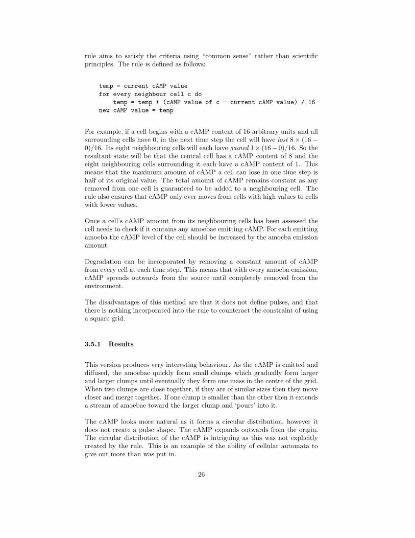
This version produces very interesting behaviour. As the cAMP is emitted anddiffused, the amoebae quickly form small clumps which gradually form largerand larger clumps until eventually they form one mass in the centre of the grid.When two clumps are close together, if they are of similar sizes then they movecloser and merge together. If one clump is smaller than the other then it extendsa stream of amoebae toward the larger clump and ‘pours’ into it.

The cAMP looks more natural as it forms a circular distribution, however itdoes not create a pulse shape. The cAMP expands outwards from the origin.The circular distribution of the cAMP is intriguing as this was not explicitlycreated by the rule. This is an example of the ability of cellular automata togive out more than was put in.

26

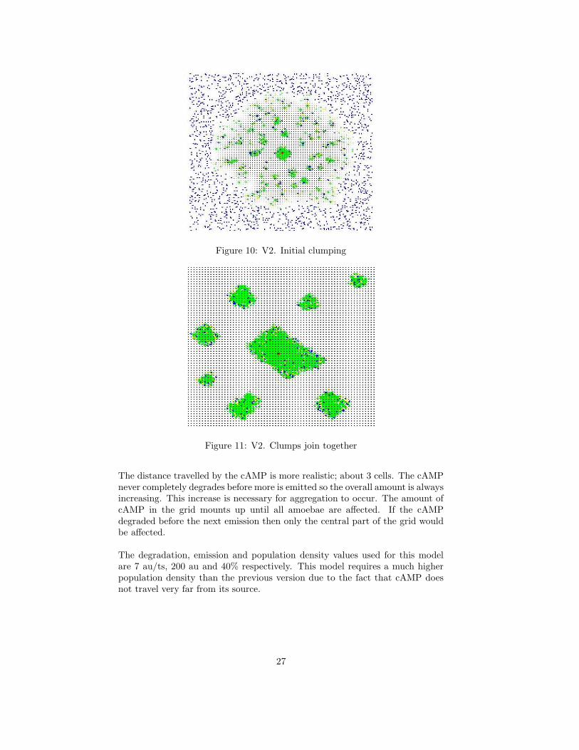
Figure 10: V2. Initial clumping

Figure 11: V2. Clumps join together

The distance travelled by the cAMP is more realistic; about 3 cells. The cAMPnever completely degrades before more is emitted so the overall amount is alwaysincreasing. This increase is necessary for aggregation to occur. The amount ofcAMP in the grid mounts up until all amoebae are affected. If the cAMPdegraded before the next emission then only the central part of the grid wouldbe affected.

The degradation, emission and population density values used for this modelare 7 au/ts, 200 au and 40% respectively. This model requires a much higherpopulation density than the previous version due to the fact that cAMP doesnot travel very far from its source.

27

3.6 Aggregation Version 3

The disadvantage of version 2 is that the cAMP does not form pulses. Ideallythere would be a way to combine the pulses of version 1 and the diffusion ofversion 2 to utilise the advantages of each method. The resolution to this wasto explicitly investigate how cAMP should move between cells. Rules are usedto described the observed patterns.

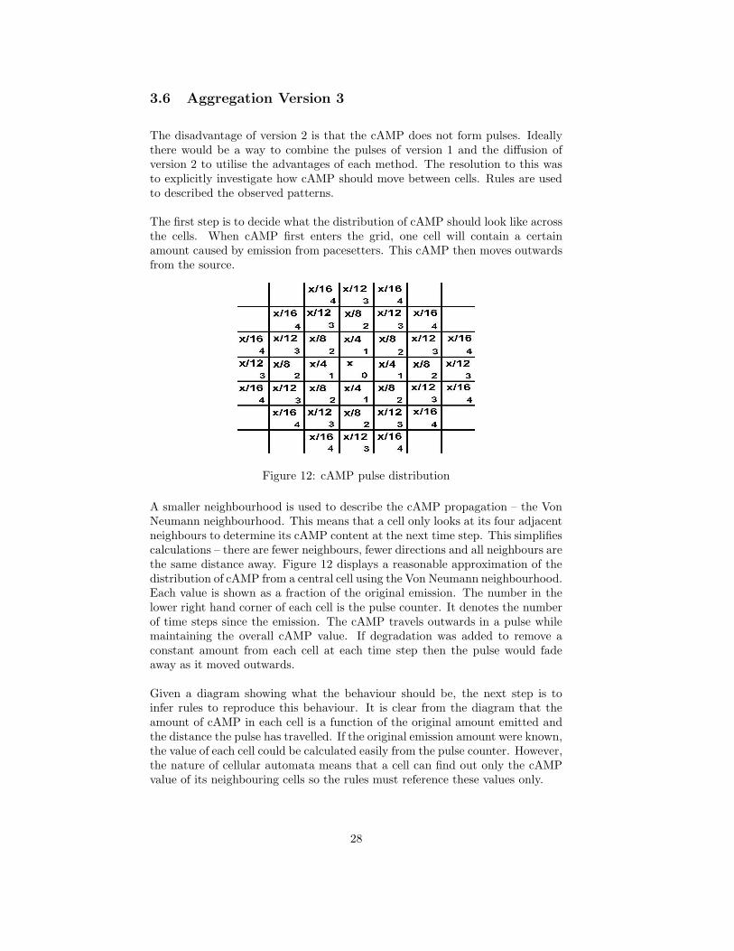
The first step is to decide what the distribution of cAMP should look like acrossthe cells. When cAMP first enters the grid, one cell will contain a certainamount caused by emission from pacesetters. This cAMP then moves outwardsfrom the source.

Figure 12: cAMP pulse distribution

A smaller neighbourhood is used to describe the cAMP propagation – the VonNeumann neighbourhood. This means that a cell only looks at its four adjacentneighbours to determine its cAMP content at the next time step. This simplifiescalculations – there are fewer neighbours, fewer directions and all neighbours arethe same distance away. Figure 12 displays a reasonable approximation of thedistribution of cAMP from a central cell using the Von Neumann neighbourhood.Each value is shown as a fraction of the original emission. The number in thelower right hand corner of each cell is the pulse counter. It denotes the numberof time steps since the emission. The cAMP travels outwards in a pulse whilemaintaining the overall cAMP value. If degradation was added to remove aconstant amount from each cell at each time step then the pulse would fadeaway as it moved outwards.

Given a diagram showing what the behaviour should be, the next step is toinfer rules to reproduce this behaviour. It is clear from the diagram that theamount of cAMP in each cell is a function of the original amount emitted andthe distance the pulse has travelled. If the original emission amount were known,the value of each cell could be calculated easily from the pulse counter. However,the nature of cellular automata means that a cell can find out only the cAMPvalue of its neighbouring cells so the rules must reference these values only.

28

Along with the cAMP value, each cell needs to store a pulse counter and adirection as part of its state. A direction is necessary to point out where thepulse came from so that cAMP always moves outwards from the source. ThecAMP update procedure must now determine new values for the cAMP content,pulse counter and direction.

Each cell sets its cAMP value to zero at the start of the update. Each neigh-bouring cell in the Von Neumann neighbourhood is checked in turn and thecAMP value increased according to the following rules.

1. If the neighbour’s counter = 0 (a pulse has just been emitted), increasecAMP value by 1/4 of the neighbour’s value.

2. If the neighbour’s direction variable is pointing here, the cAMP valueis not increased. This is because the pulse is travelling in the oppositedirection.

3. If the neighbour’s direction variable is pointing away from here, increasecAMP value by neighbour′s counter/(neighbour′s counter + 1) of theneighbour’s value. The neighbour passes most of its cAMP to this cellthen splits its remaining amount between the two cells either side of it.

4. If the neighbour’s direction variable is N, E, S or W but not pointing hereor away from here, increase cAMP value by 1/(2∗ (neighbour′s counter+1)) of the neighbour’s value. The neighbour passes most of its cAMPto the cell in the direction the pulse is travelling but half the remainingamount comes to this cell and half to the cell on its opposite side.

5. If the neighbour’s direction variable is NW, NE, SW or SE, increase cAMPvalue by 1/2 of the neighbour’s value. This is an approximation to keepthings simple. It conserves the overall amount but means that the amountis not divided equally between all cells. It should be precise enough forthis application though.

Any emissions from amoebae within the cell can then be added to obtain theoverall cAMP value.

If the value calculated is greater than zero then the direction and pulse counterneed to be set.

The direction should be set to point to the direction of the cell where cAMPwas obtained from. If cAMP was obtained from more than one neighbour thenthe directions can be averaged to produce an overall direction. For example ifa cell takes a proportion of cAMP from its north and east neighbours then itwould set its direction to NE.

The pulse counter can be set to be one greater than the counter of the cellwhere cAMP was obtained from. If cAMP was obtained from more than oneneighbour then their counters can be averaged before incrementing. Their pulsecounters are likely to be the same except in the case where there is more than

29

one pulse. This possibility occurs when the main pulse from the pacesettersexcites other amoebae who emit their own cAMP. This adds complications tothe pulse distribution. Overlapping pulses are tackled by always taking theaverage of the directions and pulse counters for each neighbouring cell cAMPwas obtained from. This may not be the most accurate method but it is thesimplest.

The code required to implement this algorithm is more complex than that of theprevious two versions. Two extra variables are added to the state of each cell tostore the pulse counter and the direction cAMP was obtained from. The cAMPupdate procedure now includes a case statement to implement the rules for thefive different cases listed above. Auxiliary functions are also added to performcalculations on directions. Degradation is incorporated in the same way as usedin version two: a constant amount is removed from each cell at every time step.

3.6.1 Results

The behaviour resulting from these complex cAMP rules is not noticeably dif-ferent to that of version 2. This seems surprising but actually with the currentbehaviour of amoebae, pulses of cAMP are not possible. This is because thepacesetter amoebae emit cAMP at every time step and so every time cAMP ismoved outward from the source, more is added to replace it. To force pulses tooccur, pacesetters must emit cAMP at certain intervals. This requires timing.

This model is no better than that of version 2 and its complexity makes itless desirable. However, it has potential to produce pulses so may prove moreeffective with the addition of timing constraints.

3.7 Timing

The timing details can be incorporated into the model by assigning a timer toeach amoeba so each cell has four independent timers. The different timingparameters are as follows:

1. There are 12 seconds between an amoeba receiving a pulse of cAMP andemitting its own pulse.

2. It takes 100 seconds for an amoeba to complete its motion in response toa cAMP pulse.

3. The pacesetter emission period is 10 minutes, which is 600 seconds.

4. The length of time between an amoeba completing its chemotactic motionand becoming responsive to cAMP once more can be anything from 2 to7 minutes. An interval of 150 seconds is used.

30

The smallest of these timings (the 12 seconds in the first item) is used as thelength of a single time step. This means that the length of time between anamoeba receiving a pulse of cAMP and emitting its own pulse is one time step.The length of time between an amoeba receiving a cAMP pulse and completingits motion in response is 100/12 = 8 time steps. The pacesetter emission periodis 600/12 = 50 time steps. The final timing constraint is the length of timebetween an amoeba completing its chemotactic motion and becoming responsiveto cAMP once more. This is 150/12 = 13 time steps.

These timings can be set as constants in the code; MOVE TIME, REST TIME,and PACE. The timing of the cAMP emission occurs immediately following thechange of state to excited so a constant is not required to time this. Thetransition rules for the different amoebae phases can then be altered to dependon the value of a timer which is incremented at each time step. One problemthat occurs at this stage is due to an amoeba taking eight time steps to completeits move. How is it possible to take eight time steps to move an amoeba betweenone cell and its neighbour? Obviously the amoebae cannot gradually make thismove, it must occur between two consecutive time steps. The compromise whichmust be made is to keep the excited amoeba in the same place until eight timesteps later when it is permitted to move. The new transition rules are now asfollows:

1. PACESETTER → PACESETTER + cAMP emission if timer = PACE;timer = (timer + 1) mod PACE

2. PACESETTER → PACESETTER otherwise; timer = (timer + 1) modPACE

3. READY → EXCITED if cAMP is detected; timer = 0

4. READY → READY otherwise

5. EXCITED → EXCITED + cAMP emission if timer = 0; timer = timer+ 1

6. EXCITED → EXCITED + trying to move if timer = MOVE TIME;

7. EXCITED → RESTING once the amoeba has moved; timer = 0

8. EXCITED → EXCITED otherwise; timer = timer + 1

9. RESTING → READY if timer = REST TIME

10. RESTING → RESTING otherwise; timer = timer + 1.

Each of the previous three models can now be extended with this new timedbehaviour.

3.8 Aggregation Version 4

This model is based on Version 1 but the timing constraints have been addedto control the behaviour of amoebae.

31

3.8.1 Results

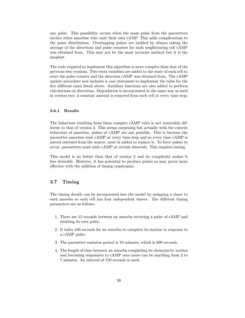
Figure 13: V4. Initial pulse with echoFigure 14: V4. Later when echoes causeexcitation

With timing added, the model no longer results in aggregation. The pulsefrom the pacesetters expands outwards and creates echoes behind it as amoebaeexcited by the pulse emit their own cAMP. Soon amoebae are becoming excitednot only from the pulses but also from the echoes. This causes the cAMPpulses to become random and distorted and means that amoebae movement isnot always towards the centre. The result is that amoebae move around butnot necessarily towards the centre and so aggregation fails. See figures 13 and14.

3.9 Aggregation Version 5

Version 2 is now extended with the timing constraints to control amoebae statetransitions.

3.9.1 Results

This results in behaviour which is fascinating to watch. It is also close inappearance to real life Dicty aggregation.

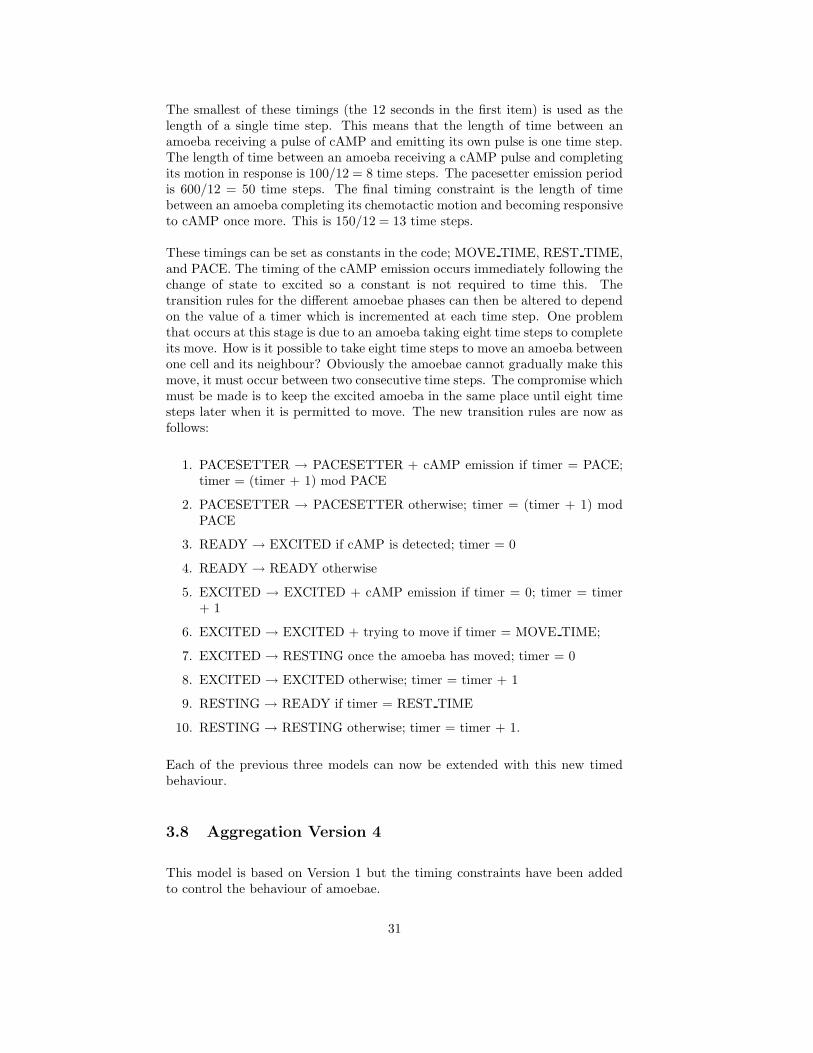
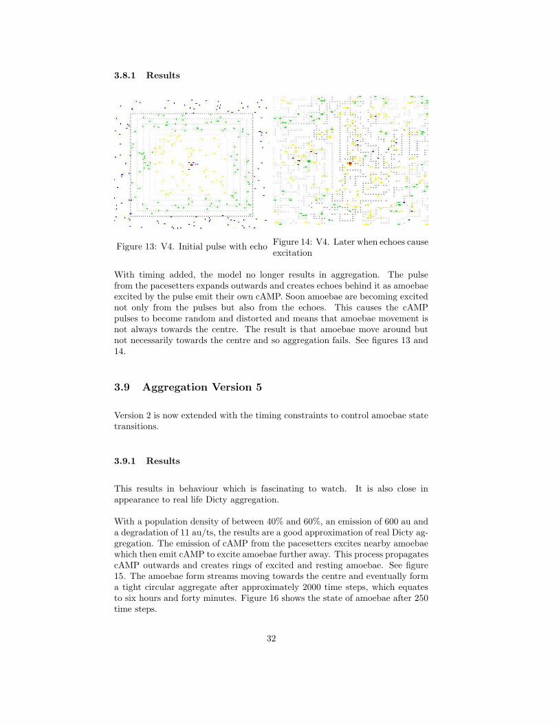
With a population density of between 40% and 60%, an emission of 600 au anda degradation of 11 au/ts, the results are a good approximation of real Dicty ag-gregation. The emission of cAMP from the pacesetters excites nearby amoebaewhich then emit cAMP to excite amoebae further away. This process propagatescAMP outwards and creates rings of excited and resting amoebae. See figure15. The amoebae form streams moving towards the centre and eventually forma tight circular aggregate after approximately 2000 time steps, which equatesto six hours and forty minutes. Figure 16 shows the state of amoebae after 250time steps.

32

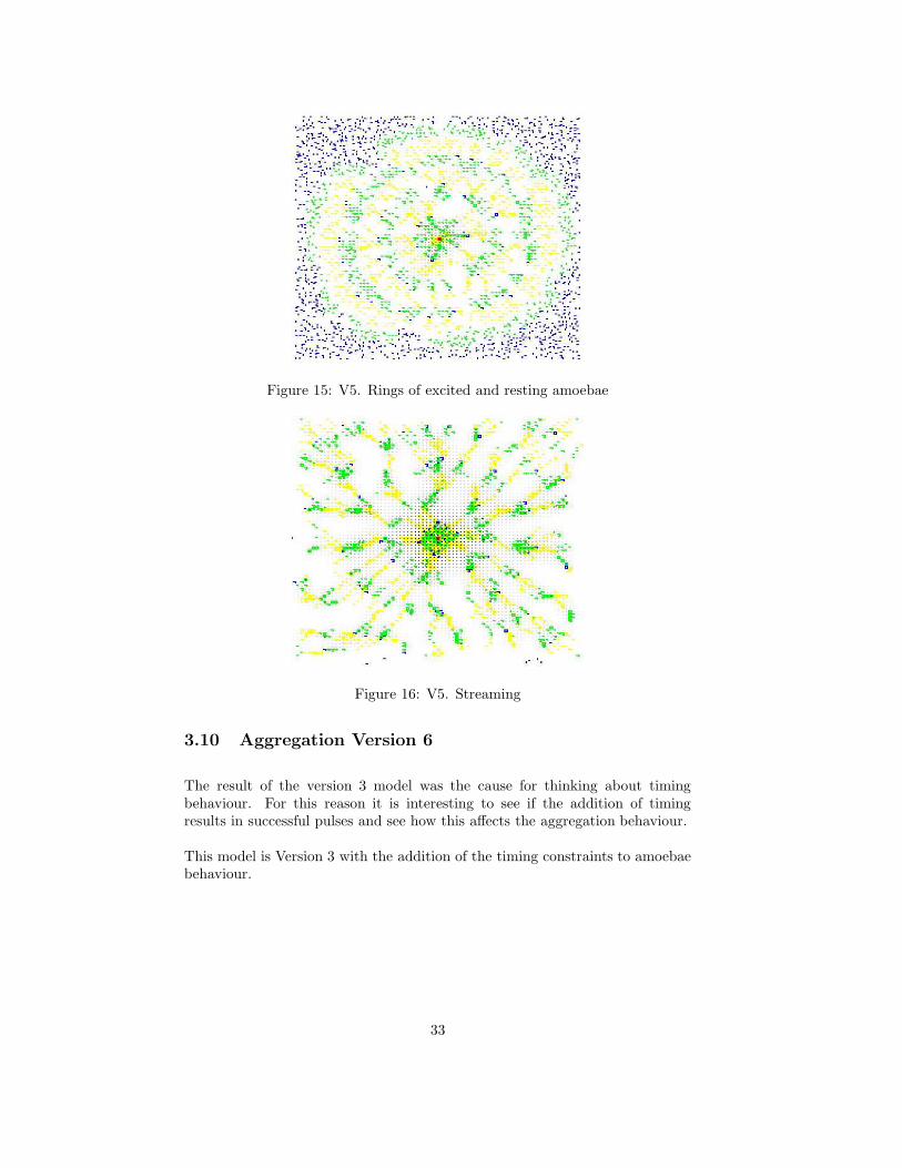
Figure 15: V5. Rings of excited and resting amoebae

Figure 16: V5. Streaming

3.10 Aggregation Version 6

The result of the version 3 model was the cause for thinking about timingbehaviour. For this reason it is interesting to see if the addition of timingresults in successful pulses and see how this affects the aggregation behaviour.

This model is Version 3 with the addition of the timing constraints to amoebaebehaviour.

33

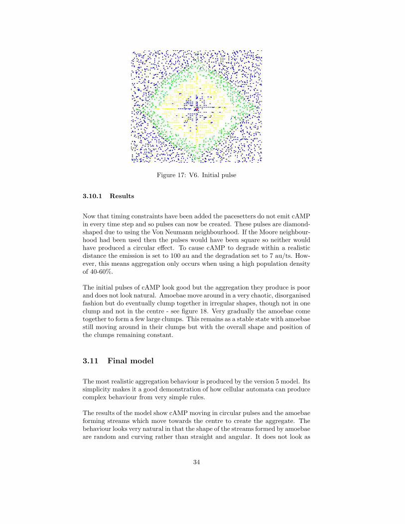
Figure 17: V6. Initial pulse

3.10.1 Results

Now that timing constraints have been added the pacesetters do not emit cAMPin every time step and so pulses can now be created. These pulses are diamond-shaped due to using the Von Neumann neighbourhood. If the Moore neighbour-hood had been used then the pulses would have been square so neither wouldhave produced a circular effect. To cause cAMP to degrade within a realisticdistance the emission is set to 100 au and the degradation set to 7 au/ts. How-ever, this means aggregation only occurs when using a high population densityof 40-60%.

The initial pulses of cAMP look good but the aggregation they produce is poorand does not look natural. Amoebae move around in a very chaotic, disorganisedfashion but do eventually clump together in irregular shapes, though not in oneclump and not in the centre - see figure 18. Very gradually the amoebae cometogether to form a few large clumps. This remains as a stable state with amoebaestill moving around in their clumps but with the overall shape and position ofthe clumps remaining constant.

3.11 Final model

The most realistic aggregation behaviour is produced by the version 5 model. Itssimplicity makes it a good demonstration of how cellular automata can producecomplex behaviour from very simple rules.

The results of the model show cAMP moving in circular pulses and the amoebaeforming streams which move towards the centre to create the aggregate. Thebehaviour looks very natural in that the shape of the streams formed by amoebaeare random and curving rather than straight and angular. It does not look as

34

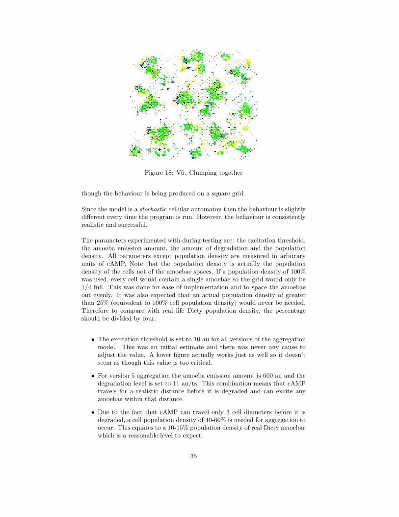
Figure 18: V6. Clumping together

though the behaviour is being produced on a square grid.

Since the model is a stochastic cellular automaton then the behaviour is slightlydifferent every time the program is run. However, the behaviour is consistentlyrealistic and successful.

The parameters experimented with during testing are: the excitation threshold,the amoeba emission amount, the amount of degradation and the populationdensity. All parameters except population density are measured in arbitraryunits of cAMP. Note that the population density is actually the populationdensity of the cells not of the amoebae spaces. If a population density of 100%was used, every cell would contain a single amoebae so the grid would only be1/4 full. This was done for ease of implementation and to space the amoebaeout evenly. It was also expected that an actual population density of greaterthan 25% (equivalent to 100% cell population density) would never be needed.Therefore to compare with real life Dicty population density, the percentageshould be divided by four.

• The excitation threshold is set to 10 au for all versions of the aggregationmodel. This was an initial estimate and there was never any cause toadjust the value. A lower figure actually works just as well so it doesn’tseem as though this value is too critical.

• For version 5 aggregation the amoeba emission amount is 600 au and thedegradation level is set to 11 au/ts. This combination means that cAMPtravels for a realistic distance before it is degraded and can excite anyamoebae within that distance.

• Due to the fact that cAMP can travel only 3 cell diameters before it isdegraded, a cell population density of 40-60% is needed for aggregation tooccur. This equates to a 10-15% population density of real Dicty amoebaewhich is a reasonable level to expect.

35

The rules used in the model are:

1. The timed state transitions of amoebae. These are shown more fully insection 3.2.6.

2. The detection of which direction amoebae should move. This is determinedby looking at each neighbour in a random order and choosing the directionof the neighbour with the highest cAMP content.

3. The movement of excited amoebae to an adjacent cell where there is room.This is controlled using the request lists described in section 3.2.1.

4. The change of direction when move requests are unsuccessful. Amoebaechange direction to either left or right (chosen randomly) of the previousdirection and make another move request.

5. The rule used to calculate the new cAMP content of a cell. This can beexpressed as:

c′ = amoebae emission +

7∑

i=0

(

neighbour[i].camp− c

16

)

,

where c is the current cAMP level of the cell and c′ is the new cAMP level.

This model can now be used as the basis to create further Dicty behaviour.

36

4 Slug migration

4.1 Dicty Slug Behaviour

Following aggregation, the amoebae in the aggregate rise up into a mound shapeuntil gravity causes the mound to topple, creating the slug.

During this motion the pacesetter amoebae would have begun in the centre ofthe aggregate and then been pushed upwards to the top of the mound. Whenthe mound topples, the pacesetters are then at the front of the slug. Pacesetterscontinue to emit cAMP and this is essential for slug movement to occur. ThecAMP waves travel along the slug from the front to the rear exciting amoebaeas they pass. The amoebae at the front of the slug then move forwards pushingthe pacesetters ahead of them. The amoebae immediately behind then have aspace to move into. This space propagates backward so the slug moves forwardin a rippling fashion.

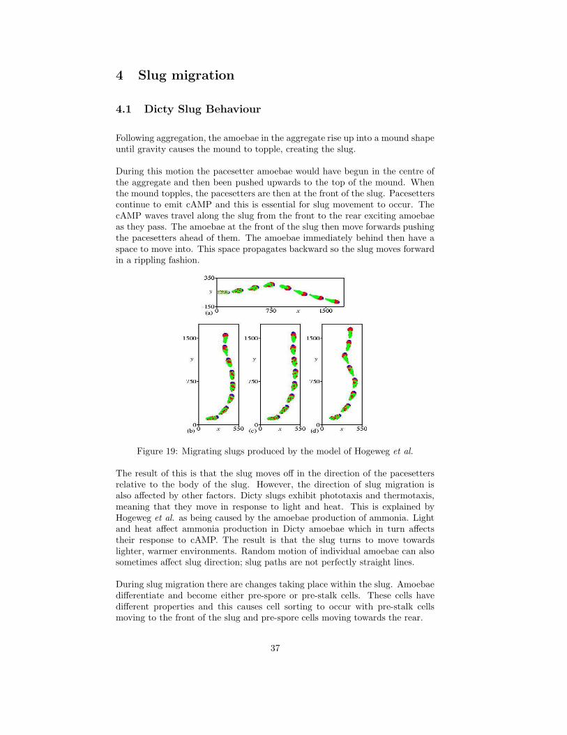
Figure 19: Migrating slugs produced by the model of Hogeweg et al.

The result of this is that the slug moves off in the direction of the pacesettersrelative to the body of the slug. However, the direction of slug migration isalso affected by other factors. Dicty slugs exhibit phototaxis and thermotaxis,meaning that they move in response to light and heat. This is explained byHogeweg et al. as being caused by the amoebae production of ammonia. Lightand heat affect ammonia production in Dicty amoebae which in turn affectstheir response to cAMP. The result is that the slug turns to move towardslighter, warmer environments. Random motion of individual amoebae can alsosometimes affect slug direction; slug paths are not perfectly straight lines.

During slug migration there are changes taking place within the slug. Amoebaedifferentiate and become either pre-spore or pre-stalk cells. These cells havedifferent properties and this causes cell sorting to occur with pre-stalk cellsmoving to the front of the slug and pre-spore cells moving towards the rear.

37

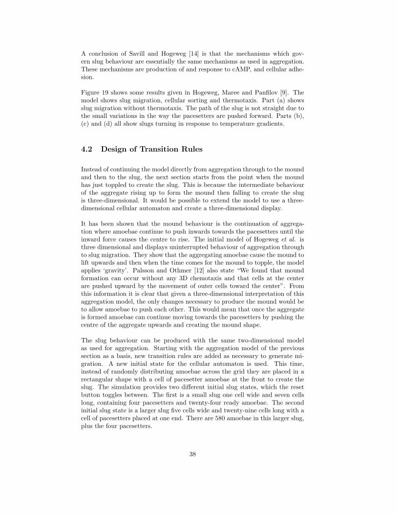
A conclusion of Savill and Hogeweg [14] is that the mechanisms which gov-ern slug behaviour are essentially the same mechanisms as used in aggregation.These mechanisms are production of and response to cAMP, and cellular adhe-sion.

Figure 19 shows some results given in Hogeweg, Maree and Panfilov [9]. Themodel shows slug migration, cellular sorting and thermotaxis. Part (a) showsslug migration without thermotaxis. The path of the slug is not straight due tothe small variations in the way the pacesetters are pushed forward. Parts (b),(c) and (d) all show slugs turning in response to temperature gradients.

4.2 Design of Transition Rules

Instead of continuing the model directly from aggregation through to the moundand then to the slug, the next section starts from the point when the moundhas just toppled to create the slug. This is because the intermediate behaviourof the aggregate rising up to form the mound then falling to create the slugis three-dimensional. It would be possible to extend the model to use a three-dimensional cellular automaton and create a three-dimensional display.

It has been shown that the mound behaviour is the continuation of aggrega-tion where amoebae continue to push inwards towards the pacesetters until theinward force causes the centre to rise. The initial model of Hogeweg et al. isthree dimensional and displays uninterrupted behaviour of aggregation throughto slug migration. They show that the aggregating amoebae cause the mound tolift upwards and then when the time comes for the mound to topple, the modelapplies ‘gravity’. Palsson and Othmer [12] also state “We found that moundformation can occur without any 3D chemotaxis and that cells at the centerare pushed upward by the movement of outer cells toward the center”. Fromthis information it is clear that given a three-dimensional interpretation of thisaggregation model, the only changes necessary to produce the mound would beto allow amoebae to push each other. This would mean that once the aggregateis formed amoebae can continue moving towards the pacesetters by pushing thecentre of the aggregate upwards and creating the mound shape.

The slug behaviour can be produced with the same two-dimensional modelas used for aggregation. Starting with the aggregation model of the previoussection as a basis, new transition rules are added as necessary to generate mi-gration. A new initial state for the cellular automaton is used. This time,instead of randomly distributing amoebae across the grid they are placed in arectangular shape with a cell of pacesetter amoebae at the front to create theslug. The simulation provides two different initial slug states, which the resetbutton toggles between. The first is a small slug one cell wide and seven cellslong, containing four pacesetters and twenty-four ready amoebae. The secondinitial slug state is a larger slug five cells wide and twenty-nine cells long with acell of pacesetters placed at one end. There are 580 amoebae in this larger slug,plus the four pacesetters.

38

4.3 Slug Version 1

The model of Hogeweg et al. concludes that slug motion is caused by amoebaepushing the pacesetters forwards. The first test was whether this could beachieved in a simpler way by allowing the pacesetters to choose the direction ofthe slug and actively moving in that direction. The theory is that the pacesettersmove off slowly while continuing to emit regular pulses of cAMP which causethe other amoebae to follow them. But does this work in practice?

The idea was implemented by coding a path for the pacesetters to follow, movingat a rate of one cell per 50 time steps. This is equivalent to one cell per cAMPpulse which is the same speed as the other amoebae can move. No other codewas altered, and no parameters changed. The small slug was used as the initialstate.

4.3.1 Results

Initially the pulses from the pacesetters excite the amoebae and cause themto cluster towards the pacesetters as they make their first steps along the pre-programmed path. However, the amoebae soon stop following the pacesettersand cluster together where the residual cAMP in the environment excites themand keeps them emitting more cAMP. The pacesetters move off alone.

The key problem seems to be that the cAMP is not being removed from theenvironment quickly enough. To combat this, the amoeba emission parameteris altered from 600 au to 70 au (the lowest possible emission which can be usedwhile still enabling the cAMP to excite neighbouring amoebae). The initialbehaviour is the same as before but after just three cAMP pulses, the pacesettershave moved too far apart from the other amoebae and the cAMP pulses nolonger reach them. This means that the amoebae remain in the ready state andso cannot move.

Intermediate values for amoebae emission all have one of the following effects:

• The emission is too high and cAMP is not completely removed from theenvironment before the next pulse. This means that amoebae do notdetect the cAMP emitted by the pacesetters over the residual cAMP inthe environment.

• The emission is too low and amoebae can only detect cAMP if they arevery close to its source. If the amoebae don’t keep close enough to thepacesetters then they can’t detect the pulses and so cannot move.

It seems that the idea of actively moving pacesetters does not work.

39

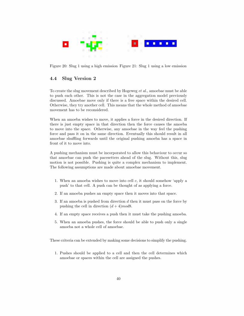
Figure 20: Slug 1 using a high emission Figure 21: Slug 1 using a low emission

4.4 Slug Version 2

To create the slug movement described by Hogeweg et al., amoebae must be ableto push each other. This is not the case in the aggregation model previouslydiscussed. Amoebae move only if there is a free space within the desired cell.Otherwise, they try another cell. This means that the whole method of amoebaemovement has to be reconsidered.

When an amoeba wishes to move, it applies a force in the desired direction. Ifthere is just empty space in that direction then the force causes the amoebato move into the space. Otherwise, any amoebae in the way feel the pushingforce and pass it on in the same direction. Eventually this should result in allamoebae shuffling forwards until the original pushing amoeba has a space infront of it to move into.

A pushing mechanism must be incorporated to allow this behaviour to occur sothat amoebae can push the pacesetters ahead of the slug. Without this, slugmotion is not possible. Pushing is quite a complex mechanism to implement.The following assumptions are made about amoebae movement.

1. When an amoeba wishes to move into cell c, it should somehow ‘apply apush’ to that cell. A push can be thought of as applying a force.

2. If an amoeba pushes an empty space then it moves into that space.

3. If an amoeba is pushed from direction d then it must pass on the force bypushing the cell in direction (d + 4)mod8.

4. If an empty space receives a push then it must take the pushing amoeba.

5. When an amoeba pushes, the force should be able to push only a singleamoeba not a whole cell of amoebae.

These criteria can be extended by making some decisions to simplify the pushing.

1. Pushes should be applied to a cell and then the cell determines whichamoebae or spaces within the cell are assigned the pushes.

40

2. Pushes can be implemented in a similar fashion to the move requests usedin aggregation by allowing amoebae to add a push to the list of a neigh-bouring cell. Cells can look at their push lists to see which neighbouringamoebae are applying pushes.

3. Cells should assign the pushes in the list to any empty spaces and amoebaewithin it. They should assign to empty spaces first so that ordinary moveswhere pushing is not required can still occur as normal.

4. Any unassigned pushes can be passed on to the next state so pushes arenever discarded, only delayed.

5. Once an amoeba has made a push it should continue waiting until a spaceis created.

These last two restrictions simplify the algorithm and avoid complexities whichcould cause amoebae to disappear or multiply. Disappearances occur if anamoeba ‘moves’ to another cell but the other cell does not allocate the amoebato it. Multiplying amoebae occur when an empty space takes on a neighbouringamoeba but that amoeba does not become an empty space. These moves mustbe carefully controlled to ensure that an amoeba becomes an empty space if andonly if an adjacent empty space becomes that amoeba.

If an amoeba never gives up on a push and continually monitors for an emptyspace being produced from the push, then an empty space assigned a push isalways able to copy the pushing amoeba into the space knowing it is safe to doso. The idea of copying any unassigned pushes to the next state is necessarybecause if excess pushes were discarded then some pushing amoebae will bewaiting indefinitely to move.

A ‘push’ can be represented as an item composed of the direction of the pushand the index of the pushing amoeba. This is the same format as the moverequests used previously. It allows identification of the pushing amoeba.

The pushing mechanism is implemented as follows. Each cell has a list as partof its state. Amoebae can add items to the lists of neighbouring cells. Whenan amoeba decides to move, it adds an item to the list of the neighbour in thedesired direction. This is no different from the move request system implementedfor the aggregation model. The change now is that when a cell checks its listit should allocate the items to the empty spaces or amoebae within the cell.While there are still spaces not yet assigned pushes and there are still pushesin the list, then the first item in the list is removed and the push assigned toa space. If there are no spaces or all have pushes assigned and the list is stillnot empty then the remaining items are assigned to any amoebae not alreadybeing pushed. Once this allocation process is complete, any remaining items inthe list are copied to the list for the next state.

A new class called Push is created to store the details of the pushes allocatedto amoebae and spaces. Each cell now has four of these Push objects as partof its state. If an amoeba or space does not have a push assigned to it then thevariables of its push object are set to a default state.

41

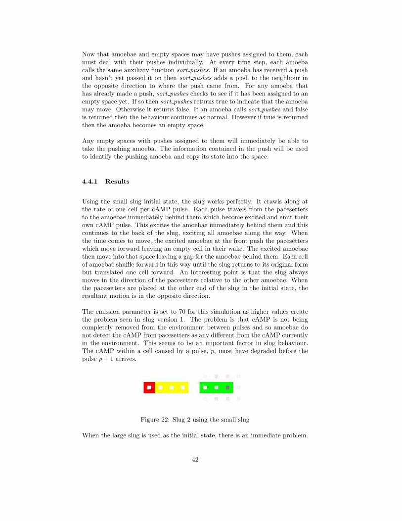
Now that amoebae and empty spaces may have pushes assigned to them, eachmust deal with their pushes individually. At every time step, each amoebacalls the same auxiliary function sort pushes. If an amoeba has received a pushand hasn’t yet passed it on then sort pushes adds a push to the neighbour inthe opposite direction to where the push came from. For any amoeba thathas already made a push, sort pushes checks to see if it has been assigned to anempty space yet. If so then sort pushes returns true to indicate that the amoebamay move. Otherwise it returns false. If an amoeba calls sort pushes and falseis returned then the behaviour continues as normal. However if true is returnedthen the amoeba becomes an empty space.

Any empty spaces with pushes assigned to them will immediately be able totake the pushing amoeba. The information contained in the push will be usedto identify the pushing amoeba and copy its state into the space.

4.4.1 Results

Using the small slug initial state, the slug works perfectly. It crawls along atthe rate of one cell per cAMP pulse. Each pulse travels from the pacesettersto the amoebae immediately behind them which become excited and emit theirown cAMP pulse. This excites the amoebae immediately behind them and thiscontinues to the back of the slug, exciting all amoebae along the way. Whenthe time comes to move, the excited amoebae at the front push the pacesetterswhich move forward leaving an empty cell in their wake. The excited amoebaethen move into that space leaving a gap for the amoebae behind them. Each cellof amoebae shuffle forward in this way until the slug returns to its original formbut translated one cell forward. An interesting point is that the slug alwaysmoves in the direction of the pacesetters relative to the other amoebae. Whenthe pacesetters are placed at the other end of the slug in the initial state, theresultant motion is in the opposite direction.

The emission parameter is set to 70 for this simulation as higher values createthe problem seen in slug version 1. The problem is that cAMP is not beingcompletely removed from the environment between pulses and so amoebae donot detect the cAMP from pacesetters as any different from the cAMP currentlyin the environment. This seems to be an important factor in slug behaviour.The cAMP within a cell caused by a pulse, p, must have degraded before thepulse p + 1 arrives.

Figure 22: Slug 2 using the small slug

When the large slug is used as the initial state, there is an immediate problem.

42

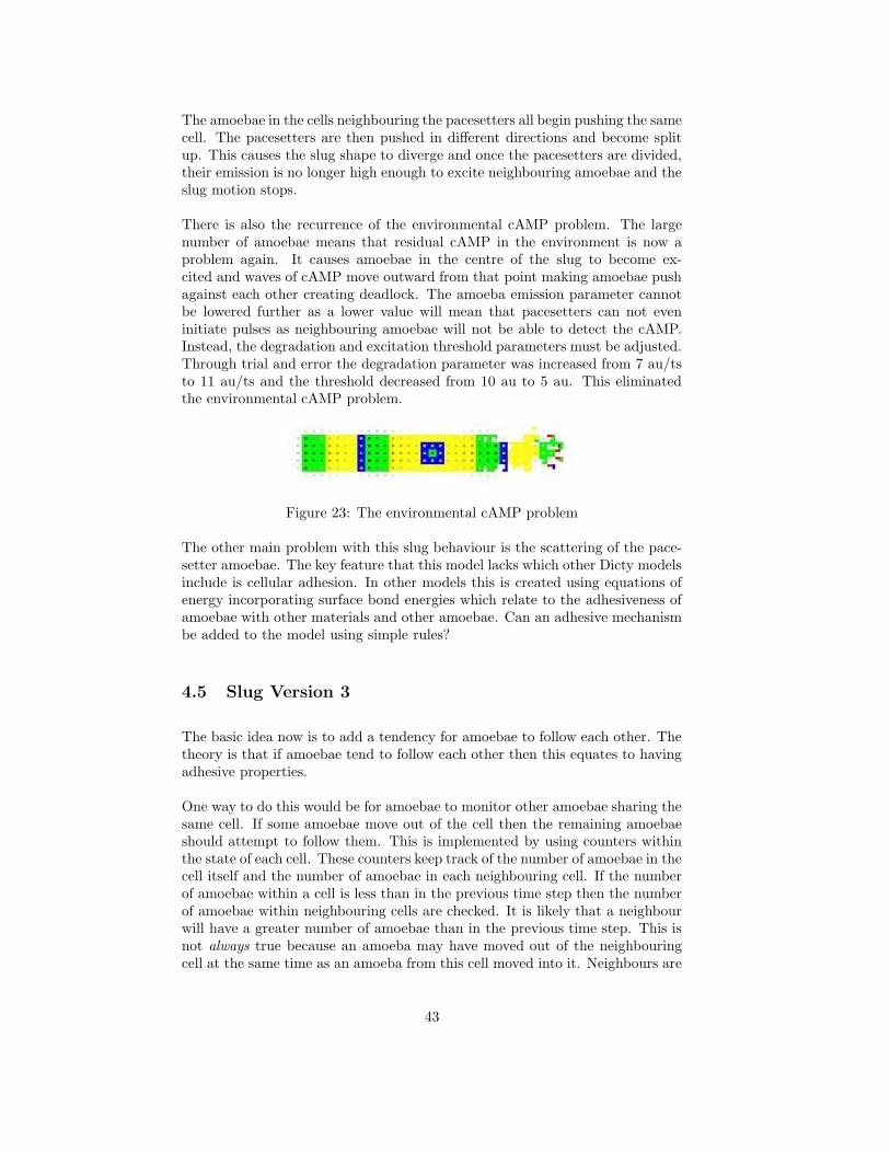
The amoebae in the cells neighbouring the pacesetters all begin pushing the samecell. The pacesetters are then pushed in different directions and become splitup. This causes the slug shape to diverge and once the pacesetters are divided,their emission is no longer high enough to excite neighbouring amoebae and theslug motion stops.

There is also the recurrence of the environmental cAMP problem. The largenumber of amoebae means that residual cAMP in the environment is now aproblem again. It causes amoebae in the centre of the slug to become ex-cited and waves of cAMP move outward from that point making amoebae pushagainst each other creating deadlock. The amoeba emission parameter cannotbe lowered further as a lower value will mean that pacesetters can not eveninitiate pulses as neighbouring amoebae will not be able to detect the cAMP.Instead, the degradation and excitation threshold parameters must be adjusted.Through trial and error the degradation parameter was increased from 7 au/tsto 11 au/ts and the threshold decreased from 10 au to 5 au. This eliminatedthe environmental cAMP problem.

Figure 23: The environmental cAMP problem

The other main problem with this slug behaviour is the scattering of the pace-setter amoebae. The key feature that this model lacks which other Dicty modelsinclude is cellular adhesion. In other models this is created using equations ofenergy incorporating surface bond energies which relate to the adhesiveness ofamoebae with other materials and other amoebae. Can an adhesive mechanismbe added to the model using simple rules?

4.5 Slug Version 3

The basic idea now is to add a tendency for amoebae to follow each other. Thetheory is that if amoebae tend to follow each other then this equates to havingadhesive properties.

One way to do this would be for amoebae to monitor other amoebae sharing thesame cell. If some amoebae move out of the cell then the remaining amoebaeshould attempt to follow them. This is implemented by using counters withinthe state of each cell. These counters keep track of the number of amoebae in thecell itself and the number of amoebae in each neighbouring cell. If the numberof amoebae within a cell is less than in the previous time step then the numberof amoebae within neighbouring cells are checked. It is likely that a neighbourwill have a greater number of amoebae than in the previous time step. This isnot always true because an amoeba may have moved out of the neighbouringcell at the same time as an amoeba from this cell moved into it. Neighbours are

43

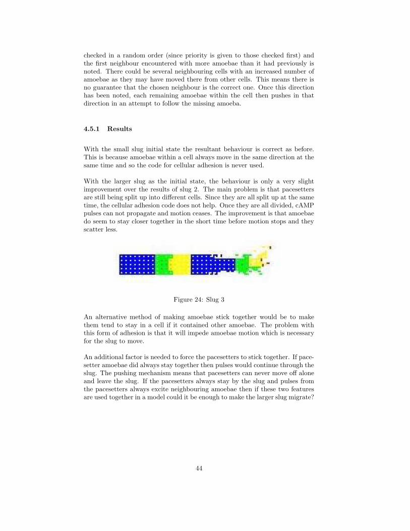
checked in a random order (since priority is given to those checked first) andthe first neighbour encountered with more amoebae than it had previously isnoted. There could be several neighbouring cells with an increased number ofamoebae as they may have moved there from other cells. This means there isno guarantee that the chosen neighbour is the correct one. Once this directionhas been noted, each remaining amoebae within the cell then pushes in thatdirection in an attempt to follow the missing amoeba.

4.5.1 Results

With the small slug initial state the resultant behaviour is correct as before.This is because amoebae within a cell always move in the same direction at thesame time and so the code for cellular adhesion is never used.

With the larger slug as the initial state, the behaviour is only a very slightimprovement over the results of slug 2. The main problem is that pacesettersare still being split up into different cells. Since they are all split up at the sametime, the cellular adhesion code does not help. Once they are all divided, cAMPpulses can not propagate and motion ceases. The improvement is that amoebaedo seem to stay closer together in the short time before motion stops and theyscatter less.

Figure 24: Slug 3

An alternative method of making amoebae stick together would be to makethem tend to stay in a cell if it contained other amoebae. The problem withthis form of adhesion is that it will impede amoebae motion which is necessaryfor the slug to move.

An additional factor is needed to force the pacesetters to stick together. If pace-setter amoebae did always stay together then pulses would continue through theslug. The pushing mechanism means that pacesetters can never move off aloneand leave the slug. If the pacesetters always stay by the slug and pulses fromthe pacesetters always excite neighbouring amoebae then if these two featuresare used together in a model could it be enough to make the larger slug migrate?

44

4.6 Slug Version 4

This next idea is to create sticky pacesetters and force them to stay together.This can be implemented by creating extra rules to deal specifically with pace-setter amoebae.

• If any pacesetter amoeba is assigned a push then all four pacesetters inthe cell pass on the push.

• Pacesetter amoebae move only if there is enough space for all the paceset-ters to move together.

• An empty space changes to a pacesetter only if there are three other emptyspaces within its cell which are taking the other three pacesetters.

4.6.1 Results

The small slug still works correctly. The larger slug initial state results in thepacesetters moving off, usually at a diagonal, and quickly separating from therest of the slug followed by only a few amoebae. The remaining slug no longersees any cAMP and stops moving. The reason the pacesetters move off ata diagonal is because they will receive pushes from their twelve neighbouringamoebae: four pushing east, four pushing north-east, and four pushing south-east. Since the pushes are ordered randomly the first push in the list is equallylikely to be north-east, south-east or east. Therefore it is twice as likely tobe a diagonal direction. The reason the pacesetters move off quickly is thatonly a single push is required to cause all pacesetters to move. However, theseproblems can be easily corrected using two adjustments.

• Pacesetters pass on a push only if all four of them are being pushed

• The direction the pacesetters push in is taken as the overall direction ofthe push on each individual pacesetter.

This results in a big improvement in the behaviour. The slug begins to moveforwards and generally stays together. However, the rear of the slug moves verylittle. The front of the slug becomes longer and thinner until eventually thefront part breaks off to create a small slug which moves off alone.

The amoebae toward the rear of the slug barely move because their pushes havelittle result. Since the amoebae wait until their push is successful, a lack ofsuccess means they do not move.

Another adjustment can be made, this time to allow amoebae to give up on apush after a certain length of time if it is not successful, i.e. it is not producingan empty space to move into. The amoeba can then randomly choose a newdirection either left or right of the previous direction and try pushing in that

45

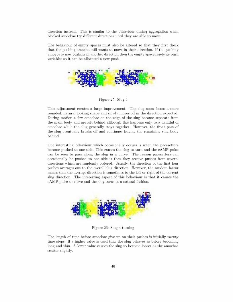
direction instead. This is similar to the behaviour during aggregation whenblocked amoebae try different directions until they are able to move.

The behaviour of empty spaces must also be altered so that they first checkthat the pushing amoeba still wants to move in their direction. If the pushingamoeba is now pushing in another direction then the empty space resets its pushvariables so it can be allocated a new push.

Figure 25: Slug 4

This adjustment creates a large improvement. The slug soon forms a morerounded, natural looking shape and slowly moves off in the direction expected.During motion a few amoebae on the edge of the slug become separate fromthe main body and are left behind although this happens only to a handful ofamoebae while the slug generally stays together. However, the front part ofthe slug eventually breaks off and continues leaving the remaining slug bodybehind.

One interesting behaviour which occasionally occurs is when the pacesettersbecome pushed to one side. This causes the slug to turn and the cAMP pulsecan be seen to pass along the slug in a curve. The reason pacesetters canoccasionally be pushed to one side is that they receive pushes from severaldirections which are randomly ordered. Usually, the direction of the first fourpushes averages out to the overall slug direction. However, the random factormeans that the average direction is sometimes to the left or right of the currentslug direction. The interesting aspect of this behaviour is that it causes thecAMP pulse to curve and the slug turns in a natural fashion.

Figure 26: Slug 4 turning

The length of time before amoebae give up on their pushes is initially twentytime steps. If a higher value is used then the slug behaves as before becominglong and thin. A lower value causes the slug to become looser as the amoebaescatter slightly.

46

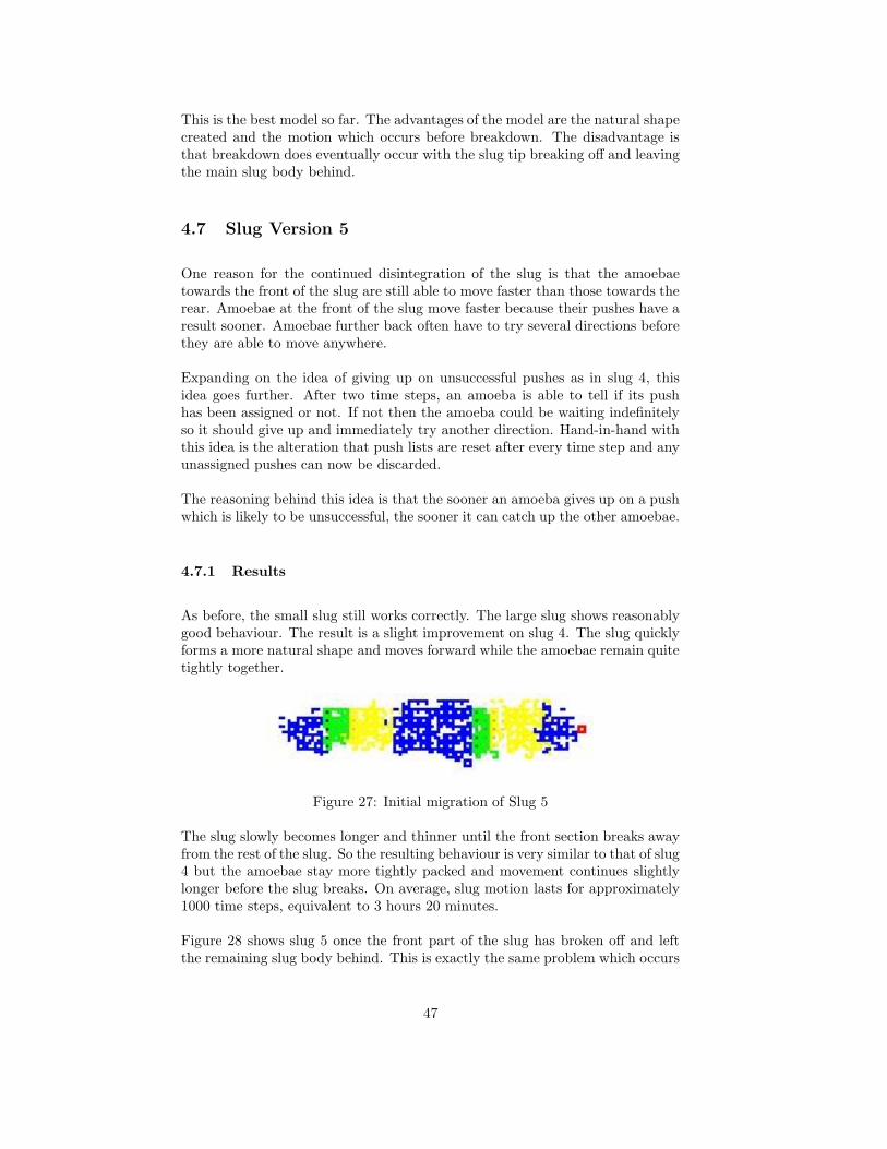
This is the best model so far. The advantages of the model are the natural shapecreated and the motion which occurs before breakdown. The disadvantage isthat breakdown does eventually occur with the slug tip breaking off and leavingthe main slug body behind.

4.7 Slug Version 5

One reason for the continued disintegration of the slug is that the amoebaetowards the front of the slug are still able to move faster than those towards therear. Amoebae at the front of the slug move faster because their pushes have aresult sooner. Amoebae further back often have to try several directions beforethey are able to move anywhere.

Expanding on the idea of giving up on unsuccessful pushes as in slug 4, thisidea goes further. After two time steps, an amoeba is able to tell if its pushhas been assigned or not. If not then the amoeba could be waiting indefinitelyso it should give up and immediately try another direction. Hand-in-hand withthis idea is the alteration that push lists are reset after every time step and anyunassigned pushes can now be discarded.

The reasoning behind this idea is that the sooner an amoeba gives up on a pushwhich is likely to be unsuccessful, the sooner it can catch up the other amoebae.

4.7.1 Results

As before, the small slug still works correctly. The large slug shows reasonablygood behaviour. The result is a slight improvement on slug 4. The slug quicklyforms a more natural shape and moves forward while the amoebae remain quitetightly together.

Figure 27: Initial migration of Slug 5

The slug slowly becomes longer and thinner until the front section breaks awayfrom the rest of the slug. So the resulting behaviour is very similar to that of slug4 but the amoebae stay more tightly packed and movement continues slightlylonger before the slug breaks. On average, slug motion lasts for approximately1000 time steps, equivalent to 3 hours 20 minutes.

Figure 28 shows slug 5 once the front part of the slug has broken off and leftthe remaining slug body behind. This is exactly the same problem which occurs

47

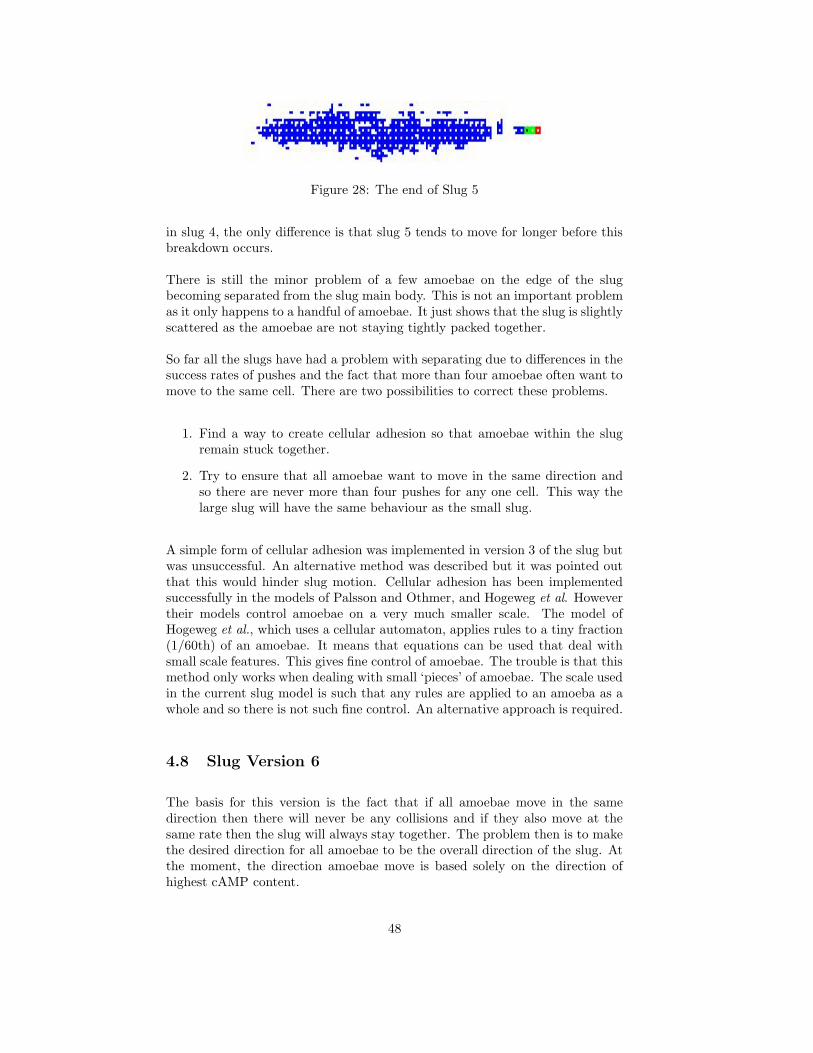
Figure 28: The end of Slug 5

in slug 4, the only difference is that slug 5 tends to move for longer before thisbreakdown occurs.

There is still the minor problem of a few amoebae on the edge of the slugbecoming separated from the slug main body. This is not an important problemas it only happens to a handful of amoebae. It just shows that the slug is slightlyscattered as the amoebae are not staying tightly packed together.

So far all the slugs have had a problem with separating due to differences in thesuccess rates of pushes and the fact that more than four amoebae often want tomove to the same cell. There are two possibilities to correct these problems.

1. Find a way to create cellular adhesion so that amoebae within the slugremain stuck together.

2. Try to ensure that all amoebae want to move in the same direction andso there are never more than four pushes for any one cell. This way thelarge slug will have the same behaviour as the small slug.

A simple form of cellular adhesion was implemented in version 3 of the slug butwas unsuccessful. An alternative method was described but it was pointed outthat this would hinder slug motion. Cellular adhesion has been implementedsuccessfully in the models of Palsson and Othmer, and Hogeweg et al. Howevertheir models control amoebae on a very much smaller scale. The model ofHogeweg et al., which uses a cellular automaton, applies rules to a tiny fraction(1/60th) of an amoebae. It means that equations can be used that deal withsmall scale features. This gives fine control of amoebae. The trouble is that thismethod only works when dealing with small ‘pieces’ of amoebae. The scale usedin the current slug model is such that any rules are applied to an amoeba as awhole and so there is not such fine control. An alternative approach is required.

4.8 Slug Version 6

The basis for this version is the fact that if all amoebae move in the samedirection then there will never be any collisions and if they also move at thesame rate then the slug will always stay together. The problem then is to makethe desired direction for all amoebae to be the overall direction of the slug. Atthe moment, the direction amoebae move is based solely on the direction ofhighest cAMP content.

48

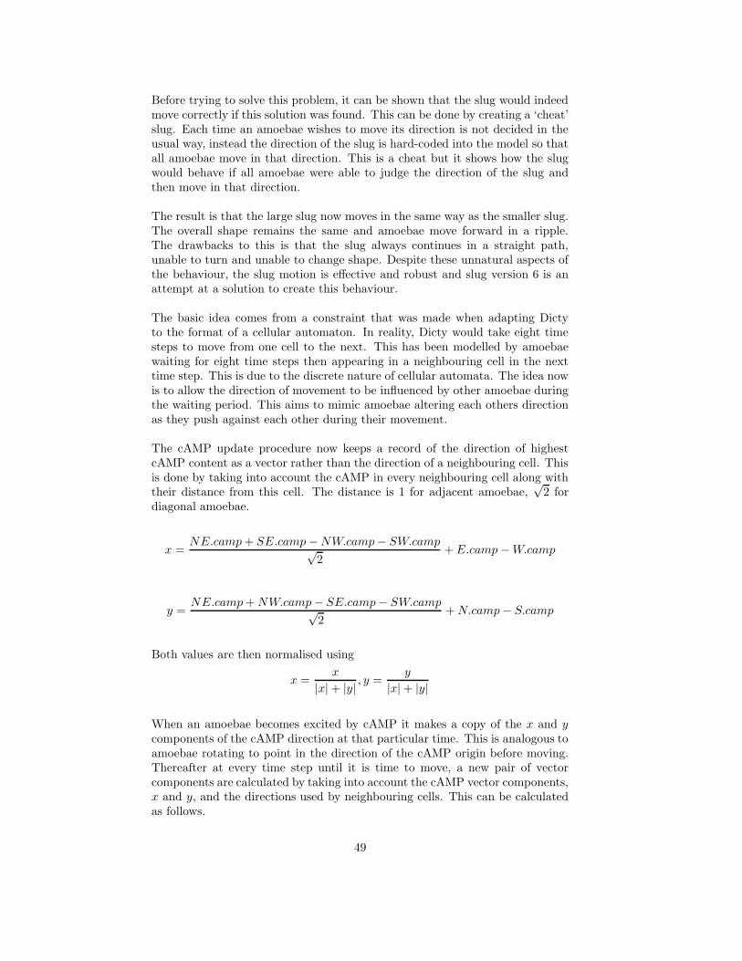
Before trying to solve this problem, it can be shown that the slug would indeedmove correctly if this solution was found. This can be done by creating a ‘cheat’slug. Each time an amoebae wishes to move its direction is not decided in theusual way, instead the direction of the slug is hard-coded into the model so thatall amoebae move in that direction. This is a cheat but it shows how the slugwould behave if all amoebae were able to judge the direction of the slug andthen move in that direction.

The result is that the large slug now moves in the same way as the smaller slug.The overall shape remains the same and amoebae move forward in a ripple.The drawbacks to this is that the slug always continues in a straight path,unable to turn and unable to change shape. Despite these unnatural aspects ofthe behaviour, the slug motion is effective and robust and slug version 6 is anattempt at a solution to create this behaviour.

The basic idea comes from a constraint that was made when adapting Dictyto the format of a cellular automaton. In reality, Dicty would take eight timesteps to move from one cell to the next. This has been modelled by amoebaewaiting for eight time steps then appearing in a neighbouring cell in the nexttime step. This is due to the discrete nature of cellular automata. The idea nowis to allow the direction of movement to be influenced by other amoebae duringthe waiting period. This aims to mimic amoebae altering each others directionas they push against each other during their movement.

The cAMP update procedure now keeps a record of the direction of highestcAMP content as a vector rather than the direction of a neighbouring cell. Thisis done by taking into account the cAMP in every neighbouring cell along withtheir distance from this cell. The distance is 1 for adjacent amoebae,

√2 for

diagonal amoebae.

x =NE.camp + SE.camp − NW.camp − SW.camp√

2+ E.camp − W.camp

y =NE.camp + NW.camp − SE.camp − SW.camp√

2+ N.camp − S.camp

Both values are then normalised using

x =x

|x| + |y| , y =y

|x| + |y|

When an amoebae becomes excited by cAMP it makes a copy of the x and ycomponents of the cAMP direction at that particular time. This is analogous toamoebae rotating to point in the direction of the cAMP origin before moving.Thereafter at every time step until it is time to move, a new pair of vectorcomponents are calculated by taking into account the cAMP vector components,x and y, and the directions used by neighbouring cells. This can be calculatedas follows.

49

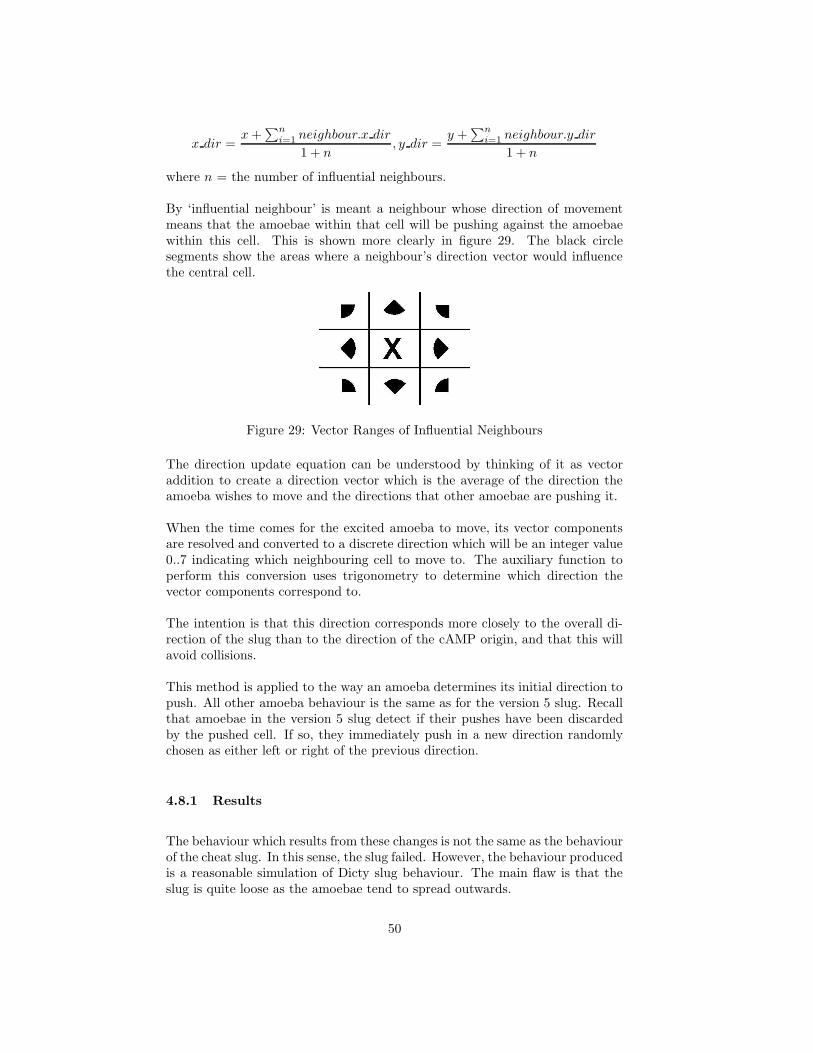
x dir =x +

∑n

i=1 neighbour.x dir

1 + n, y dir =

y +∑n

i=1 neighbour.y dir

1 + n

where n = the number of influential neighbours.

By ‘influential neighbour’ is meant a neighbour whose direction of movementmeans that the amoebae within that cell will be pushing against the amoebaewithin this cell. This is shown more clearly in figure 29. The black circlesegments show the areas where a neighbour’s direction vector would influencethe central cell.

Figure 29: Vector Ranges of Influential Neighbours

The direction update equation can be understood by thinking of it as vectoraddition to create a direction vector which is the average of the direction theamoeba wishes to move and the directions that other amoebae are pushing it.

When the time comes for the excited amoeba to move, its vector componentsare resolved and converted to a discrete direction which will be an integer value0..7 indicating which neighbouring cell to move to. The auxiliary function toperform this conversion uses trigonometry to determine which direction thevector components correspond to.

The intention is that this direction corresponds more closely to the overall di-rection of the slug than to the direction of the cAMP origin, and that this willavoid collisions.

This method is applied to the way an amoeba determines its initial direction topush. All other amoeba behaviour is the same as for the version 5 slug. Recallthat amoebae in the version 5 slug detect if their pushes have been discardedby the pushed cell. If so, they immediately push in a new direction randomlychosen as either left or right of the previous direction.

4.8.1 Results

The behaviour which results from these changes is not the same as the behaviourof the cheat slug. In this sense, the slug failed. However, the behaviour producedis a reasonable simulation of Dicty slug behaviour. The main flaw is that theslug is quite loose as the amoebae tend to spread outwards.

50

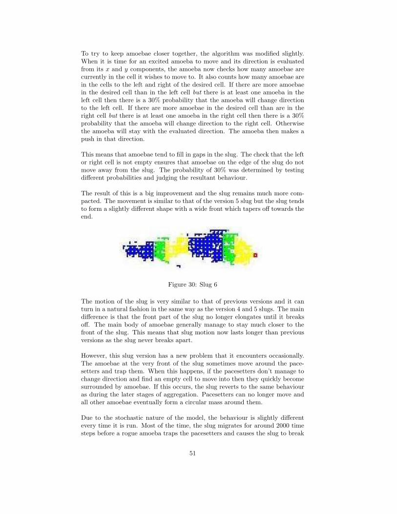
To try to keep amoebae closer together, the algorithm was modified slightly.When it is time for an excited amoeba to move and its direction is evaluatedfrom its x and y components, the amoeba now checks how many amoebae arecurrently in the cell it wishes to move to. It also counts how many amoebae arein the cells to the left and right of the desired cell. If there are more amoebaein the desired cell than in the left cell but there is at least one amoeba in theleft cell then there is a 30% probability that the amoeba will change directionto the left cell. If there are more amoebae in the desired cell than are in theright cell but there is at least one amoeba in the right cell then there is a 30%probability that the amoeba will change direction to the right cell. Otherwisethe amoeba will stay with the evaluated direction. The amoeba then makes apush in that direction.

This means that amoebae tend to fill in gaps in the slug. The check that the leftor right cell is not empty ensures that amoebae on the edge of the slug do notmove away from the slug. The probability of 30% was determined by testingdifferent probabilities and judging the resultant behaviour.

The result of this is a big improvement and the slug remains much more com-pacted. The movement is similar to that of the version 5 slug but the slug tendsto form a slightly different shape with a wide front which tapers off towards theend.

Figure 30: Slug 6

The motion of the slug is very similar to that of previous versions and it canturn in a natural fashion in the same way as the version 4 and 5 slugs. The maindifference is that the front part of the slug no longer elongates until it breaksoff. The main body of amoebae generally manage to stay much closer to thefront of the slug. This means that slug motion now lasts longer than previousversions as the slug never breaks apart.

However, this slug version has a new problem that it encounters occasionally.The amoebae at the very front of the slug sometimes move around the pace-setters and trap them. When this happens, if the pacesetters don’t manage tochange direction and find an empty cell to move into then they quickly becomesurrounded by amoebae. If this occurs, the slug reverts to the same behaviouras during the later stages of aggregation. Pacesetters can no longer move andall other amoebae eventually form a circular mass around them.

Due to the stochastic nature of the model, the behaviour is slightly differentevery time it is run. Most of the time, the slug migrates for around 2000 timesteps before a rogue amoeba traps the pacesetters and causes the slug to break

51

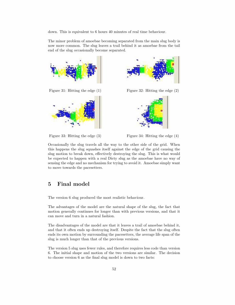
down. This is equivalent to 6 hours 40 minutes of real time behaviour.

The minor problem of amoebae becoming separated from the main slug body isnow more common. The slug leaves a trail behind it as amoebae from the tailend of the slug occasionally become separated.

Figure 31: Hitting the edge (1) Figure 32: Hitting the edge (2)

Figure 33: Hitting the edge (3) Figure 34: Hitting the edge (4)

Occasionally the slug travels all the way to the other side of the grid. Whenthis happens the slug squashes itself against the edge of the grid causing theslug motion to break down, effectively destroying the slug. This is what wouldbe expected to happen with a real Dicty slug as the amoebae have no way ofsensing the edge and no mechanism for trying to avoid it. Amoebae simply wantto move towards the pacesetters.

5 Final model

The version 6 slug produced the most realistic behaviour.

The advantages of the model are the natural shape of the slug, the fact thatmotion generally continues for longer than with previous versions, and that itcan move and turn in a natural fashion.

The disadvantages of the model are that it leaves a trail of amoebae behind it,and that it often ends up destroying itself. Despite the fact that the slug oftenends its own motion by surrounding the pacesetters, the average life span of theslug is much longer than that of the previous versions.

The version 5 slug uses fewer rules, and therefore requires less code than version6. The initial shape and motion of the two versions are similar. The decisionto choose version 6 as the final slug model is down to two facts:

52

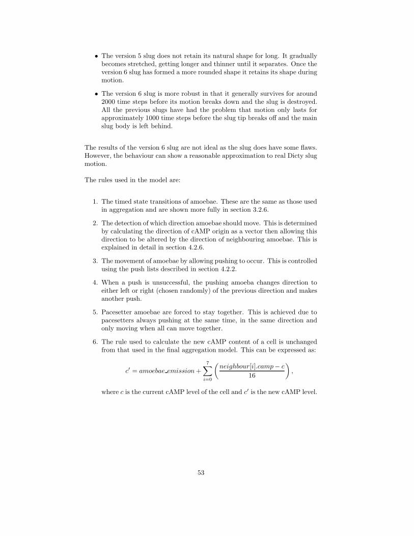
• The version 5 slug does not retain its natural shape for long. It graduallybecomes stretched, getting longer and thinner until it separates. Once theversion 6 slug has formed a more rounded shape it retains its shape duringmotion.

• The version 6 slug is more robust in that it generally survives for around2000 time steps before its motion breaks down and the slug is destroyed.All the previous slugs have had the problem that motion only lasts forapproximately 1000 time steps before the slug tip breaks off and the mainslug body is left behind.

The results of the version 6 slug are not ideal as the slug does have some flaws.However, the behaviour can show a reasonable approximation to real Dicty slugmotion.

The rules used in the model are:

1. The timed state transitions of amoebae. These are the same as those usedin aggregation and are shown more fully in section 3.2.6.

2. The detection of which direction amoebae should move. This is determinedby calculating the direction of cAMP origin as a vector then allowing thisdirection to be altered by the direction of neighbouring amoebae. This isexplained in detail in section 4.2.6.

3. The movement of amoebae by allowing pushing to occur. This is controlledusing the push lists described in section 4.2.2.

4. When a push is unsuccessful, the pushing amoeba changes direction toeither left or right (chosen randomly) of the previous direction and makesanother push.

5. Pacesetter amoebae are forced to stay together. This is achieved due topacesetters always pushing at the same time, in the same direction andonly moving when all can move together.

6. The rule used to calculate the new cAMP content of a cell is unchangedfrom that used in the final aggregation model. This can be expressed as:

c′ = amoebae emission +

7∑

i=0

(

neighbour[i].camp− c

16

)

,

where c is the current cAMP level of the cell and c′ is the new cAMP level.

53

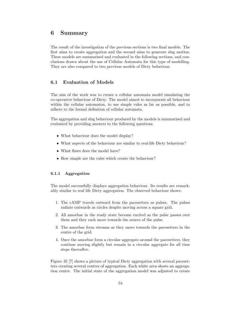
6 Summary

The result of the investigation of the previous sections is two final models. Thefirst aims to create aggregation and the second aims to generate slug motion.These models are summarised and evaluated in the following sections, and con-clusions drawn about the use of Cellular Automata for this type of modelling.They are also compared to two previous models of Dicty behaviour.

6.1 Evaluation of Models

The aim of the work was to create a cellular automata model simulating theco-operative behaviour of Dicty. The model aimed to incorporate all behaviourwithin the cellular automaton, to use simple rules as far as possible, and toadhere to the formal definition of cellular automata.

The aggregation and slug behaviour produced by the models is summarised andevaluated by providing answers to the following questions.

• What behaviour does the model display?

• What aspects of the behaviour are similar to real-life Dicty behaviour?

• What flaws does the model have?

• How simple are the rules which create the behaviour?

6.1.1 Aggregation

The model successfully displays aggregation behaviour. Its results are remark-ably similar to real life Dicty aggregation. The observed behaviour shows:

1. The cAMP travels outward from the pacesetters as pulses. The pulsesradiate outwards as circles despite moving across a square grid.

2. All amoebae in the ready state become excited as the pulse passes overthem and they each move towards the source of the pulse.

3. The amoebae form streams as they move towards the pacesetters in thecentre of the grid.

4. Once the amoebae form a circular aggregate around the pacesetters, theycontinue moving slightly but remain in a circular aggregate for all timesteps thereafter.

Figure 35 [7] shows a picture of typical Dicty aggregation with several paceset-ters creating several centres of aggregation. Each white area shows an aggrega-tion centre. The initial state of the aggregation model was adjusted to create

54

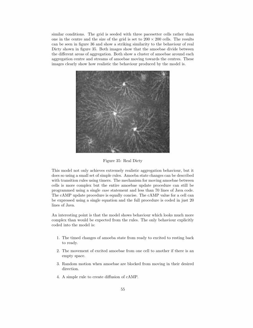
similar conditions. The grid is seeded with three pacesetter cells rather thanone in the centre and the size of the grid is set to 200 × 200 cells. The resultscan be seen in figure 36 and show a striking similarity to the behaviour of realDicty shown in figure 35. Both images show that the amoebae divide betweenthe different areas of aggregation. Both show a cluster of amoebae around eachaggregation centre and streams of amoebae moving towards the centres. Theseimages clearly show how realistic the behaviour produced by the model is.

Figure 35: Real Dicty

This model not only achieves extremely realistic aggregation behaviour, but itdoes so using a small set of simple rules. Amoeba state changes can be describedwith transition rules using timers. The mechanism for moving amoebae betweencells is more complex but the entire amoebae update procedure can still beprogrammed using a single case statement and less than 70 lines of Java code.The cAMP update procedure is equally concise. The cAMP value for a cell canbe expressed using a single equation and the full procedure is coded in just 20lines of Java.

An interesting point is that the model shows behaviour which looks much morecomplex than would be expected from the rules. The only behaviour explicitlycoded into the model is:

1. The timed changes of amoeba state from ready to excited to resting backto ready.

2. The movement of excited amoebae from one cell to another if there is anempty space.

3. Random motion when amoebae are blocked from moving in their desireddirection.

4. A simple rule to create diffusion of cAMP.

55

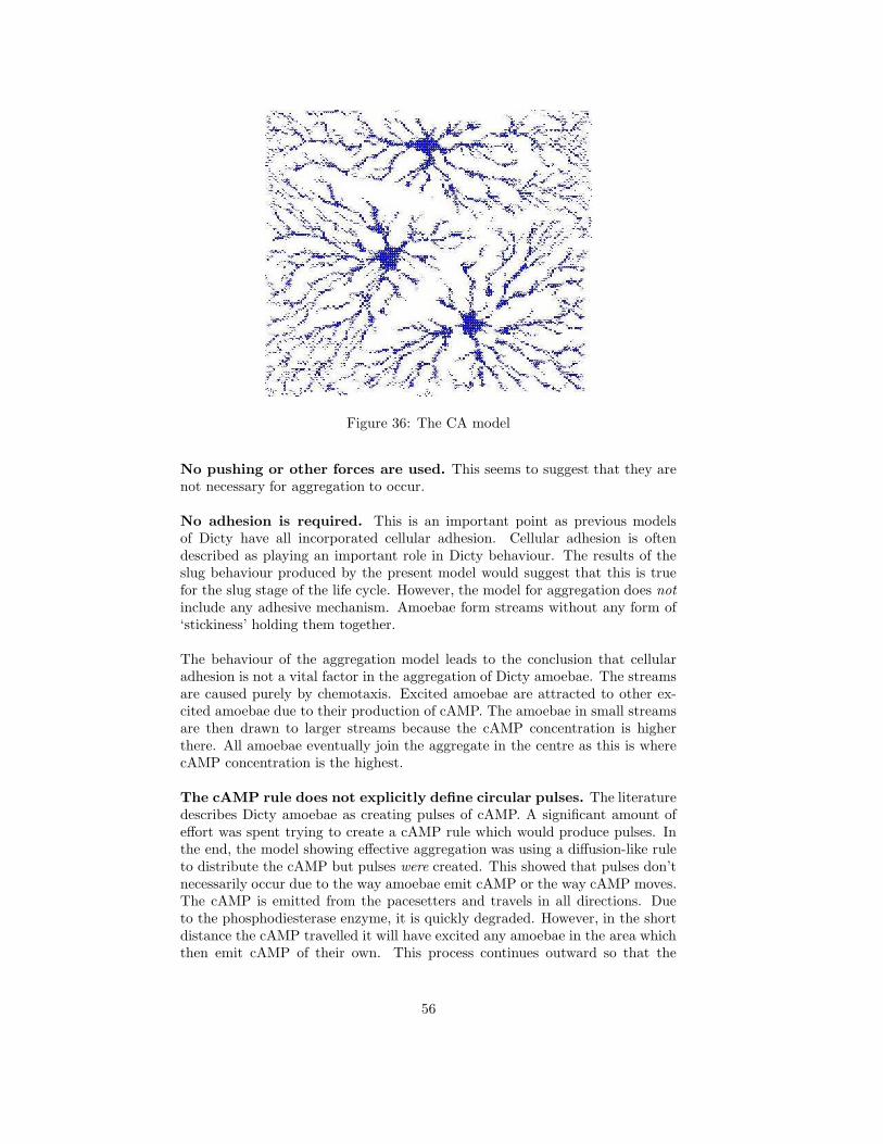
Figure 36: The CA model

No pushing or other forces are used. This seems to suggest that they arenot necessary for aggregation to occur.

No adhesion is required. This is an important point as previous modelsof Dicty have all incorporated cellular adhesion. Cellular adhesion is oftendescribed as playing an important role in Dicty behaviour. The results of theslug behaviour produced by the present model would suggest that this is truefor the slug stage of the life cycle. However, the model for aggregation does not

include any adhesive mechanism. Amoebae form streams without any form of‘stickiness’ holding them together.

The behaviour of the aggregation model leads to the conclusion that cellularadhesion is not a vital factor in the aggregation of Dicty amoebae. The streamsare caused purely by chemotaxis. Excited amoebae are attracted to other ex-cited amoebae due to their production of cAMP. The amoebae in small streamsare then drawn to larger streams because the cAMP concentration is higherthere. All amoebae eventually join the aggregate in the centre as this is wherecAMP concentration is the highest.

The cAMP rule does not explicitly define circular pulses. The literaturedescribes Dicty amoebae as creating pulses of cAMP. A significant amount ofeffort was spent trying to create a cAMP rule which would produce pulses. Inthe end, the model showing effective aggregation was using a diffusion-like ruleto distribute the cAMP but pulses were created. This showed that pulses don’tnecessarily occur due to the way amoebae emit cAMP or the way cAMP moves.The cAMP is emitted from the pacesetters and travels in all directions. Dueto the phosphodiesterase enzyme, it is quickly degraded. However, in the shortdistance the cAMP travelled it will have excited any amoebae in the area whichthen emit cAMP of their own. This process continues outward so that the

56

cAMP looks as though it is moving outward in a circular pulse. The refractoryphase of amoebae ensures that pulses only ever travel outwards. The enzymeproduced by the amoebae ensures that cAMP is degraded following the passingof a pulse.

The model takes approximately 2000 time steps to complete aggregation froma random distribution of ready amoebae to a circular aggregate, which equatesto 6 hours 40 minutes. This is in the correct range for real Dicty aggregationwhich takes 6 to 12 hours.

Although there is a high similarity between the model behaviour and real Dictyaggregation, the simulation is not perfect. The main flaws in the behaviour aredue to the restrictions of using a discrete model.

• Every amoeba is entirely described by the state of a single cell and isdisplayed as a small rectangle. Real life Dicty amoebae can change shapeand can rotate. The amoebae in this model cannot. During aggregationreal Dicty amoebae become elongated as they move to join the aggregateand form streams. The amoebae in the model remain as rectangles andtheir rotation depends only on their position within the cell.

• Each amoeba can travel in only one of eight directions. The amoebaein the model often form straight lines in some places during aggregation.The lines formed by real Dicty amoebae are not likely to be so perfectlystraight so this factor can make the behaviour look slightly unnatural.

• Each cell uses a space half the size of an amoeba to display the cAMPlevel. This does not affect the behaviour of the model but it does affectthe way the amoebae look. Even in the centre of the aggregate where allcells are full of amoebae, these small areas within each cell may look likeempty spaces. It causes the output to look less like a picture of real Dictyaggregation.

6.1.2 Slug migration

The final slug model produces reasonable behaviour. It is not perfect but itdoes show many realistic features. The observed behaviour shows:

1. The slug quickly changes from its initial compact, rectangular shape to alooser, rounded and more natural looking shape.

2. The pulse of cAMP initiated by the pacesetters passes along the slug in awave.

3. Each pulse of cAMP causes the amoebae within the slug to move and pushthe pacesetters forward.

4. The slug moves in the direction of the pacesetters relative to the slug body.

57

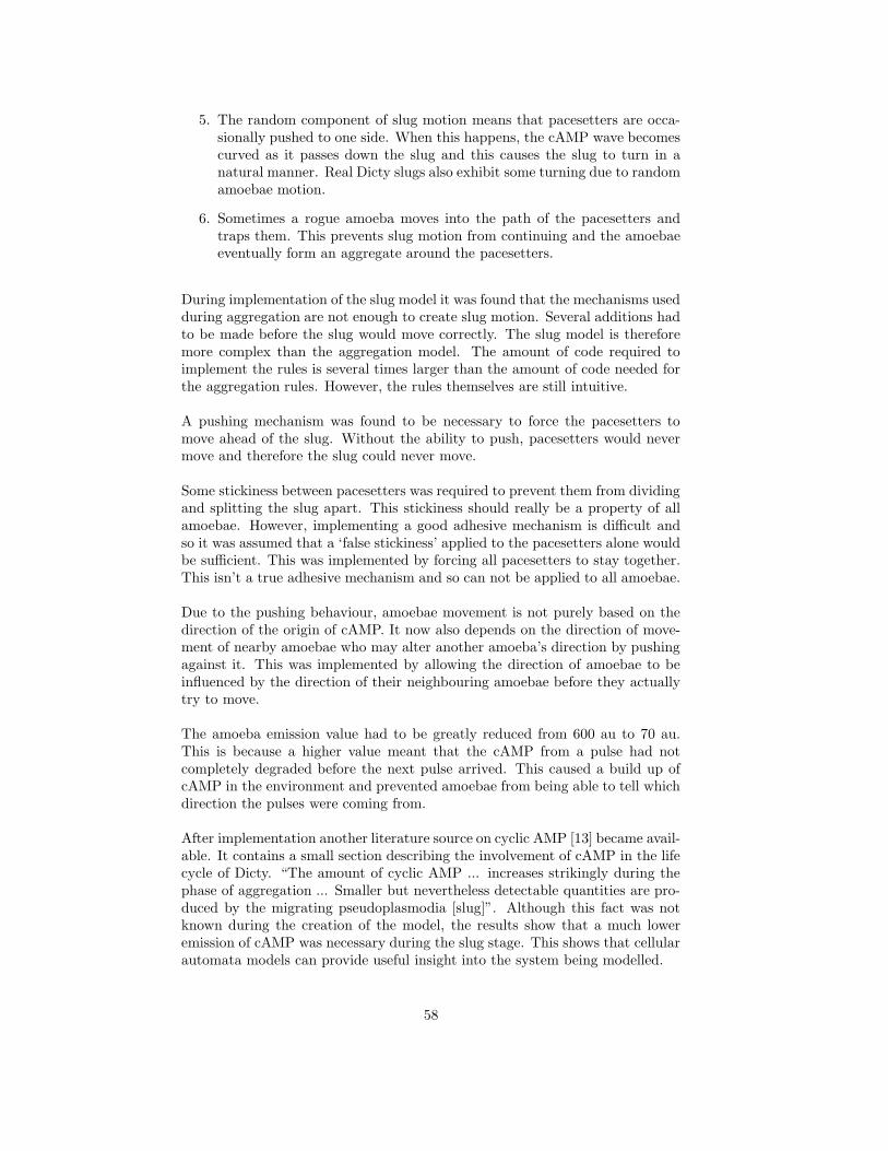
5. The random component of slug motion means that pacesetters are occa-sionally pushed to one side. When this happens, the cAMP wave becomescurved as it passes down the slug and this causes the slug to turn in anatural manner. Real Dicty slugs also exhibit some turning due to randomamoebae motion.

6. Sometimes a rogue amoeba moves into the path of the pacesetters andtraps them. This prevents slug motion from continuing and the amoebaeeventually form an aggregate around the pacesetters.

During implementation of the slug model it was found that the mechanisms usedduring aggregation are not enough to create slug motion. Several additions hadto be made before the slug would move correctly. The slug model is thereforemore complex than the aggregation model. The amount of code required toimplement the rules is several times larger than the amount of code needed forthe aggregation rules. However, the rules themselves are still intuitive.

A pushing mechanism was found to be necessary to force the pacesetters tomove ahead of the slug. Without the ability to push, pacesetters would nevermove and therefore the slug could never move.

Some stickiness between pacesetters was required to prevent them from dividingand splitting the slug apart. This stickiness should really be a property of allamoebae. However, implementing a good adhesive mechanism is difficult andso it was assumed that a ‘false stickiness’ applied to the pacesetters alone wouldbe sufficient. This was implemented by forcing all pacesetters to stay together.This isn’t a true adhesive mechanism and so can not be applied to all amoebae.

Due to the pushing behaviour, amoebae movement is not purely based on thedirection of the origin of cAMP. It now also depends on the direction of move-ment of nearby amoebae who may alter another amoeba’s direction by pushingagainst it. This was implemented by allowing the direction of amoebae to beinfluenced by the direction of their neighbouring amoebae before they actuallytry to move.

The amoeba emission value had to be greatly reduced from 600 au to 70 au.This is because a higher value meant that the cAMP from a pulse had notcompletely degraded before the next pulse arrived. This caused a build up ofcAMP in the environment and prevented amoebae from being able to tell whichdirection the pulses were coming from.

After implementation another literature source on cyclic AMP [13] became avail-able. It contains a small section describing the involvement of cAMP in the lifecycle of Dicty. “The amount of cyclic AMP ... increases strikingly during thephase of aggregation ... Smaller but nevertheless detectable quantities are pro-duced by the migrating pseudoplasmodia [slug]”. Although this fact was notknown during the creation of the model, the results show that a much loweremission of cAMP was necessary during the slug stage. This shows that cellularautomata models can provide useful insight into the system being modelled.

58

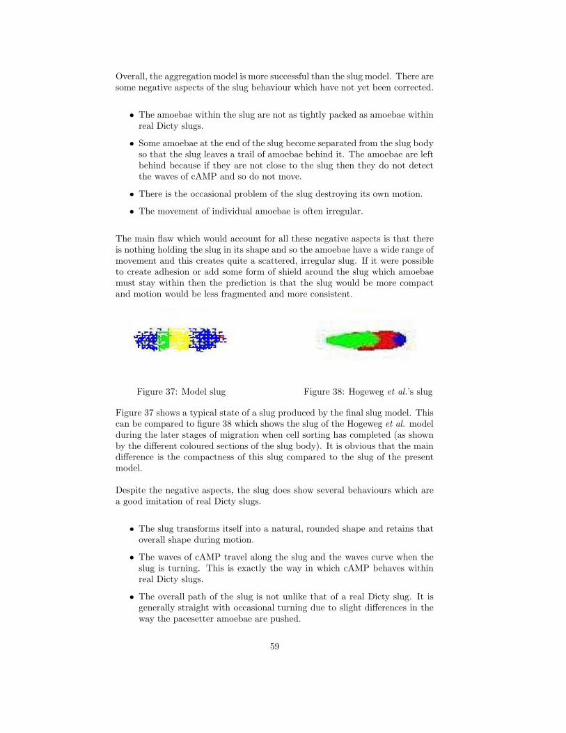
Overall, the aggregation model is more successful than the slug model. There aresome negative aspects of the slug behaviour which have not yet been corrected.

• The amoebae within the slug are not as tightly packed as amoebae withinreal Dicty slugs.

• Some amoebae at the end of the slug become separated from the slug bodyso that the slug leaves a trail of amoebae behind it. The amoebae are leftbehind because if they are not close to the slug then they do not detectthe waves of cAMP and so do not move.

• There is the occasional problem of the slug destroying its own motion.

• The movement of individual amoebae is often irregular.

The main flaw which would account for all these negative aspects is that thereis nothing holding the slug in its shape and so the amoebae have a wide range ofmovement and this creates quite a scattered, irregular slug. If it were possibleto create adhesion or add some form of shield around the slug which amoebaemust stay within then the prediction is that the slug would be more compactand motion would be less fragmented and more consistent.

Figure 37: Model slug Figure 38: Hogeweg et al.’s slug

Figure 37 shows a typical state of a slug produced by the final slug model. Thiscan be compared to figure 38 which shows the slug of the Hogeweg et al. modelduring the later stages of migration when cell sorting has completed (as shownby the different coloured sections of the slug body). It is obvious that the maindifference is the compactness of this slug compared to the slug of the presentmodel.

Despite the negative aspects, the slug does show several behaviours which area good imitation of real Dicty slugs.

• The slug transforms itself into a natural, rounded shape and retains thatoverall shape during motion.

• The waves of cAMP travel along the slug and the waves curve when theslug is turning. This is exactly the way in which cAMP behaves withinreal Dicty slugs.

• The overall path of the slug is not unlike that of a real Dicty slug. It isgenerally straight with occasional turning due to slight differences in theway the pacesetter amoebae are pushed.

59

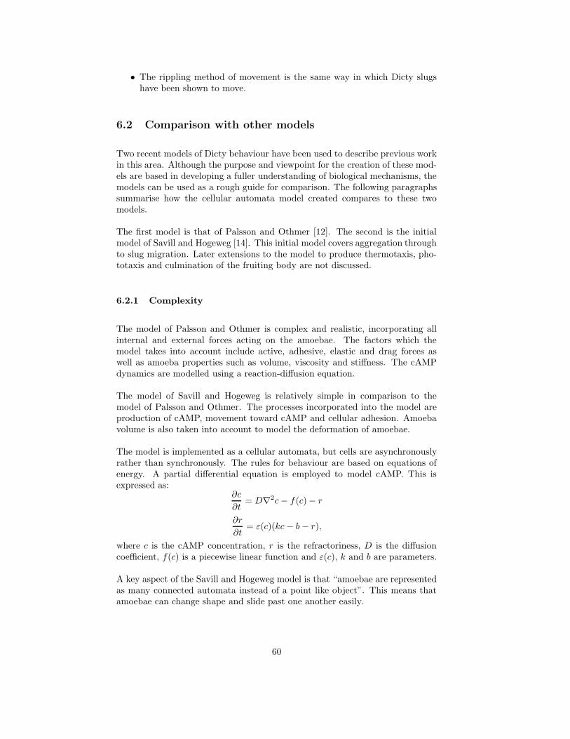
• The rippling method of movement is the same way in which Dicty slugshave been shown to move.

6.2 Comparison with other models

Two recent models of Dicty behaviour have been used to describe previous workin this area. Although the purpose and viewpoint for the creation of these mod-els are based in developing a fuller understanding of biological mechanisms, themodels can be used as a rough guide for comparison. The following paragraphssummarise how the cellular automata model created compares to these twomodels.

The first model is that of Palsson and Othmer [12]. The second is the initialmodel of Savill and Hogeweg [14]. This initial model covers aggregation throughto slug migration. Later extensions to the model to produce thermotaxis, pho-totaxis and culmination of the fruiting body are not discussed.

6.2.1 Complexity

The model of Palsson and Othmer is complex and realistic, incorporating allinternal and external forces acting on the amoebae. The factors which themodel takes into account include active, adhesive, elastic and drag forces aswell as amoeba properties such as volume, viscosity and stiffness. The cAMPdynamics are modelled using a reaction-diffusion equation.

The model of Savill and Hogeweg is relatively simple in comparison to themodel of Palsson and Othmer. The processes incorporated into the model areproduction of cAMP, movement toward cAMP and cellular adhesion. Amoebavolume is also taken into account to model the deformation of amoebae.

The model is implemented as a cellular automata, but cells are asynchronouslyrather than synchronously. The rules for behaviour are based on equations ofenergy. A partial differential equation is employed to model cAMP. This isexpressed as:

∂c

∂t= D∇2c − f(c) − r

∂r

∂t= ε(c)(kc − b − r),

where c is the cAMP concentration, r is the refractoriness, D is the diffusioncoefficient, f(c) is a piecewise linear function and ε(c), k and b are parameters.

A key aspect of the Savill and Hogeweg model is that “amoebae are representedas many connected automata instead of a point like object”. This means thatamoebae can change shape and slide past one another easily.

60

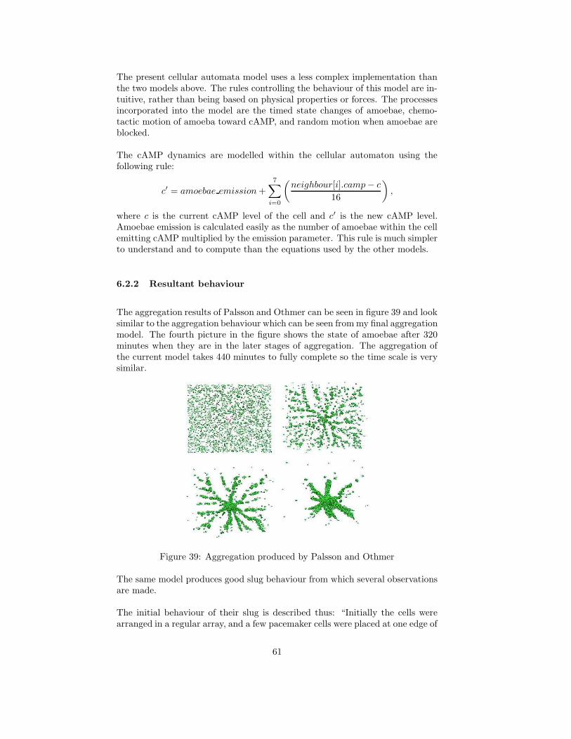
The present cellular automata model uses a less complex implementation thanthe two models above. The rules controlling the behaviour of this model are in-tuitive, rather than being based on physical properties or forces. The processesincorporated into the model are the timed state changes of amoebae, chemo-tactic motion of amoeba toward cAMP, and random motion when amoebae areblocked.

The cAMP dynamics are modelled within the cellular automaton using thefollowing rule:

c′ = amoebae emission +

7∑

i=0

(

neighbour[i].camp− c

16

)

,

where c is the current cAMP level of the cell and c′ is the new cAMP level.Amoebae emission is calculated easily as the number of amoebae within the cellemitting cAMP multiplied by the emission parameter. This rule is much simplerto understand and to compute than the equations used by the other models.

6.2.2 Resultant behaviour

The aggregation results of Palsson and Othmer can be seen in figure 39 and looksimilar to the aggregation behaviour which can be seen from my final aggregationmodel. The fourth picture in the figure shows the state of amoebae after 320minutes when they are in the later stages of aggregation. The aggregation ofthe current model takes 440 minutes to fully complete so the time scale is verysimilar.

Figure 39: Aggregation produced by Palsson and Othmer

The same model produces good slug behaviour from which several observationsare made.

The initial behaviour of their slug is described thus: “Initially the cells werearranged in a regular array, and a few pacemaker cells were placed at one edge of

61

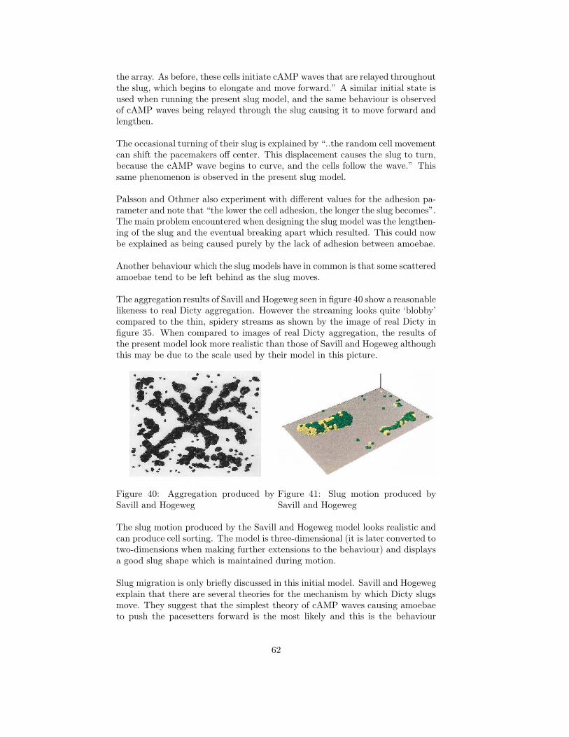
the array. As before, these cells initiate cAMP waves that are relayed throughoutthe slug, which begins to elongate and move forward.” A similar initial state isused when running the present slug model, and the same behaviour is observedof cAMP waves being relayed through the slug causing it to move forward andlengthen.

The occasional turning of their slug is explained by “..the random cell movementcan shift the pacemakers off center. This displacement causes the slug to turn,because the cAMP wave begins to curve, and the cells follow the wave.” Thissame phenomenon is observed in the present slug model.

Palsson and Othmer also experiment with different values for the adhesion pa-rameter and note that “the lower the cell adhesion, the longer the slug becomes”.The main problem encountered when designing the slug model was the lengthen-ing of the slug and the eventual breaking apart which resulted. This could nowbe explained as being caused purely by the lack of adhesion between amoebae.

Another behaviour which the slug models have in common is that some scatteredamoebae tend to be left behind as the slug moves.

The aggregation results of Savill and Hogeweg seen in figure 40 show a reasonablelikeness to real Dicty aggregation. However the streaming looks quite ‘blobby’compared to the thin, spidery streams as shown by the image of real Dicty infigure 35. When compared to images of real Dicty aggregation, the results ofthe present model look more realistic than those of Savill and Hogeweg althoughthis may be due to the scale used by their model in this picture.

Figure 40: Aggregation produced bySavill and Hogeweg

Figure 41: Slug motion produced bySavill and Hogeweg

The slug motion produced by the Savill and Hogeweg model looks realistic andcan produce cell sorting. The model is three-dimensional (it is later converted totwo-dimensions when making further extensions to the behaviour) and displaysa good slug shape which is maintained during motion.

Slug migration is only briefly discussed in this initial model. Savill and Hogewegexplain that there are several theories for the mechanism by which Dicty slugsmove. They suggest that the simplest theory of cAMP waves causing amoebaeto push the pacesetters forward is the most likely and this is the behaviour

62

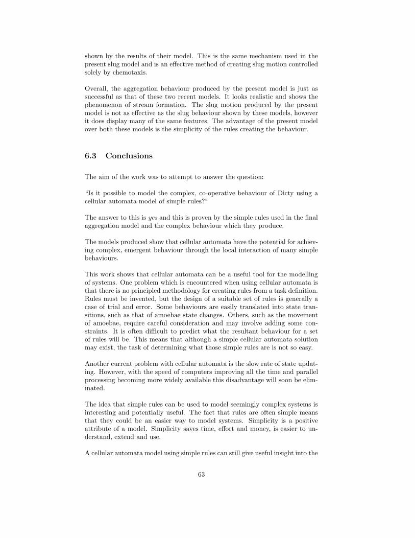
shown by the results of their model. This is the same mechanism used in thepresent slug model and is an effective method of creating slug motion controlledsolely by chemotaxis.

Overall, the aggregation behaviour produced by the present model is just assuccessful as that of these two recent models. It looks realistic and shows thephenomenon of stream formation. The slug motion produced by the presentmodel is not as effective as the slug behaviour shown by these models, howeverit does display many of the same features. The advantage of the present modelover both these models is the simplicity of the rules creating the behaviour.

6.3 Conclusions

The aim of the work was to attempt to answer the question:

“Is it possible to model the complex, co-operative behaviour of Dicty using acellular automata model of simple rules?”

The answer to this is yes and this is proven by the simple rules used in the finalaggregation model and the complex behaviour which they produce.

The models produced show that cellular automata have the potential for achiev-ing complex, emergent behaviour through the local interaction of many simplebehaviours.

This work shows that cellular automata can be a useful tool for the modellingof systems. One problem which is encountered when using cellular automata isthat there is no principled methodology for creating rules from a task definition.Rules must be invented, but the design of a suitable set of rules is generally acase of trial and error. Some behaviours are easily translated into state tran-sitions, such as that of amoebae state changes. Others, such as the movementof amoebae, require careful consideration and may involve adding some con-straints. It is often difficult to predict what the resultant behaviour for a setof rules will be. This means that although a simple cellular automata solutionmay exist, the task of determining what those simple rules are is not so easy.

Another current problem with cellular automata is the slow rate of state updat-ing. However, with the speed of computers improving all the time and parallelprocessing becoming more widely available this disadvantage will soon be elim-inated.

The idea that simple rules can be used to model seemingly complex systems isinteresting and potentially useful. The fact that rules are often simple meansthat they could be an easier way to model systems. Simplicity is a positiveattribute of a model. Simplicity saves time, effort and money, is easier to un-derstand, extend and use.

A cellular automata model using simple rules can still give useful insight into the

63

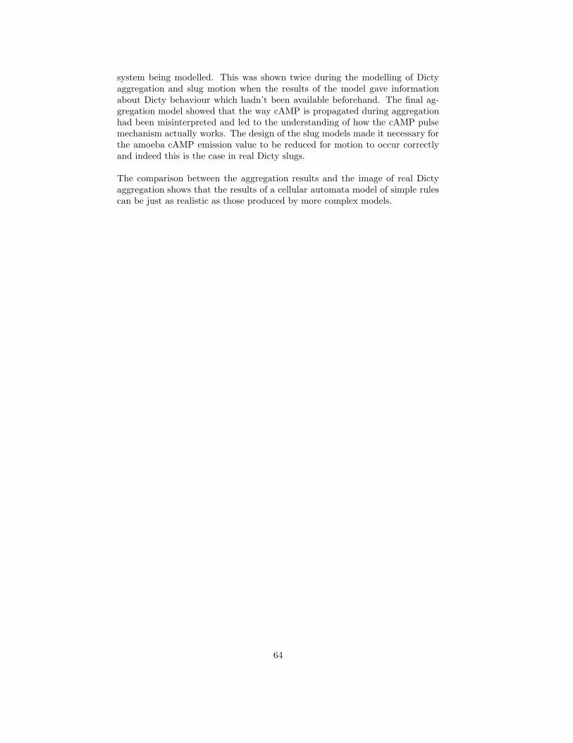
system being modelled. This was shown twice during the modelling of Dictyaggregation and slug motion when the results of the model gave informationabout Dicty behaviour which hadn’t been available beforehand. The final ag-gregation model showed that the way cAMP is propagated during aggregationhad been misinterpreted and led to the understanding of how the cAMP pulsemechanism actually works. The design of the slug models made it necessary forthe amoeba cAMP emission value to be reduced for motion to occur correctlyand indeed this is the case in real Dicty slugs.

The comparison between the aggregation results and the image of real Dictyaggregation shows that the results of a cellular automata model of simple rulescan be just as realistic as those produced by more complex models.

64

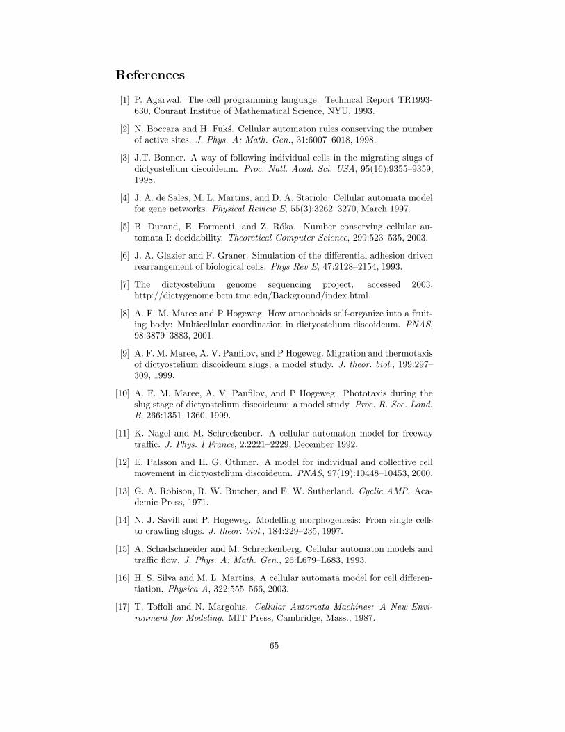
References

[1] P. Agarwal. The cell programming language. Technical Report TR1993-630, Courant Institue of Mathematical Science, NYU, 1993.

[2] N. Boccara and H. Fuks. Cellular automaton rules conserving the numberof active sites. J. Phys. A: Math. Gen., 31:6007–6018, 1998.

[3] J.T. Bonner. A way of following individual cells in the migrating slugs ofdictyostelium discoideum. Proc. Natl. Acad. Sci. USA, 95(16):9355–9359,1998.

[4] J. A. de Sales, M. L. Martins, and D. A. Stariolo. Cellular automata modelfor gene networks. Physical Review E, 55(3):3262–3270, March 1997.

[5] B. Durand, E. Formenti, and Z. Roka. Number conserving cellular au-tomata I: decidability. Theoretical Computer Science, 299:523–535, 2003.

[6] J. A. Glazier and F. Graner. Simulation of the differential adhesion drivenrearrangement of biological cells. Phys Rev E, 47:2128–2154, 1993.

[7] The dictyostelium genome sequencing project, accessed 2003.http://dictygenome.bcm.tmc.edu/Background/index.html.

[8] A. F. M. Maree and P Hogeweg. How amoeboids self-organize into a fruit-ing body: Multicellular coordination in dictyostelium discoideum. PNAS,98:3879–3883, 2001.

[9] A. F. M. Maree, A. V. Panfilov, and P Hogeweg. Migration and thermotaxisof dictyostelium discoideum slugs, a model study. J. theor. biol., 199:297–309, 1999.

[10] A. F. M. Maree, A. V. Panfilov, and P Hogeweg. Phototaxis during theslug stage of dictyostelium discoideum: a model study. Proc. R. Soc. Lond.

B, 266:1351–1360, 1999.

[11] K. Nagel and M. Schreckenber. A cellular automaton model for freewaytraffic. J. Phys. I France, 2:2221–2229, December 1992.

[12] E. Palsson and H. G. Othmer. A model for individual and collective cellmovement in dictyostelium discoideum. PNAS, 97(19):10448–10453, 2000.

[13] G. A. Robison, R. W. Butcher, and E. W. Sutherland. Cyclic AMP. Aca-demic Press, 1971.

[14] N. J. Savill and P. Hogeweg. Modelling morphogenesis: From single cellsto crawling slugs. J. theor. biol., 184:229–235, 1997.

[15] A. Schadschneider and M. Schreckenberg. Cellular automaton models andtraffic flow. J. Phys. A: Math. Gen., 26:L679–L683, 1993.

[16] H. S. Silva and M. L. Martins. A cellular automata model for cell differen-tiation. Physica A, 322:555–566, 2003.

[17] T. Toffoli and N. Margolus. Cellular Automata Machines: A New Envi-

ronment for Modeling. MIT Press, Cambridge, Mass., 1987.

65

[18] B.N. Vasiev, P. Hogeweg, and A.V. Panfilov. Simulation of dictyosteliumdiscoideum aggregation via reaction-diffusion model. Phys. Rev. Lett.,73:31733176, 1994.

[19] J.R. Weimar, J.J. Tyson, and L.T. Watson. Diffusion and wave propagationin cellular automaton models of excitable media. Physica D, 55:309–327,1992.

66

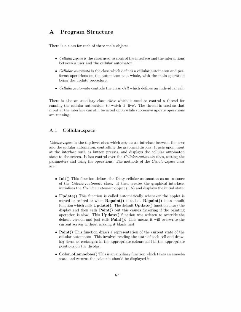
A Program Structure

There is a class for each of three main objects.

• Cellular space is the class used to control the interface and the interactionsbetween a user and the cellular automaton.

• Cellular automata is the class which defines a cellular automaton and per-forms operations on the automaton as a whole, with the main operationbeing the update procedure.

• Cellular automata controls the class Cell which defines an individual cell.

There is also an auxiliary class Alive which is used to control a thread forrunning the cellular automaton, to watch it ‘live’. The thread is used so thatinput at the interface can still be acted upon while successive update operationsare running.

A.1 Cellular space

Cellular space is the top-level class which acts as an interface between the userand the cellular automaton, controlling the graphical display. It acts upon inputat the interface such as button presses, and displays the cellular automatonstate to the screen. It has control over the Cellular automata class, setting theparameters and using the operations. The methods of the Cellular space classare:

• Init() This function defines the Dicty cellular automaton as an instanceof the Cellular automata class. It then creates the graphical interface,initialises the Cellular automata object (CA) and displays the initial state.

• Update() This function is called automatically whenever the applet ismoved or resized or when Repaint() is called. Repaint() is an inbuiltfunction which calls Update(). The default Update() function clears thedisplay and then calls Paint() but this causes flickering if the paintingoperation is slow. This Update() function was written to override thedefault version and just calls Paint(). This means it will overwrite thecurrent screen without making it blank first.

• Paint() This function draws a representation of the current state of thecellular automaton. This involves reading the state of each cell and draw-ing them as rectangles in the appropriate colours and in the appropriatepositions on the display.

• Color of amoebae() This is an auxiliary function which takes an amoebastate and returns the colour it should be displayed in.

67

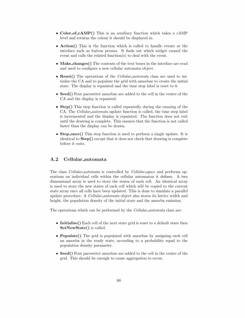
• Color of cAMP() This is an auxiliary function which takes a cAMPlevel and returns the colour it should be displayed in.

• Action() This is the function which is called to handle events at theinterface such as button presses. It finds out which widget caused theevent and calls the related function(s) to deal with the event.

• Make changes() The contents of the text boxes in the interface are readand used to configure a new cellular automata object.

• Reset() The operations of the Cellular automata class are used to ini-tialise the CA and to populate the grid with amoebae to create the initialstate. The display is repainted and the time step label is reset to 0.

• Seed() Four pacesetter amoebae are added to the cell in the centre of theCA and the display is repainted.

• Step() This step function is called repeatedly during the running of theCA. The Cellular automata update function is called, the time step labelis incremented and the display is repainted. The function does not exituntil the drawing is complete. This ensures that the function is not calledfaster than the display can be drawn.

• Step once() This step function is used to perform a single update. It isidentical to Step() except that it does not check that drawing is completebefore it exits.

A.2 Cellular automata

The class Cellular automata is controlled by Cellular space and performs op-erations on individual cells within the cellular automaton it defines. A twodimensional array is used to store the states of each cell. An identical arrayis used to store the new states of each cell which will be copied to the currentstate array once all cells have been updated. This is done to simulate a parallelupdate procedure. A Cellular automata object also stores its lattice width andheight, the population density of the initial state and the amoeba emission.

The operations which can be performed by the Cellular automata class are:

• Initialise() Each cell of the next state grid is reset to a default state thenSetNewState() is called.

• Populate() The grid is populated with amoebae by assigning each cellan amoeba in the ready state, according to a probability equal to thepopulation density parameter.

• Seed() Four pacesetter amoebae are added to the cell in the centre of thegrid. This should be enough to cause aggregation to occur.

68

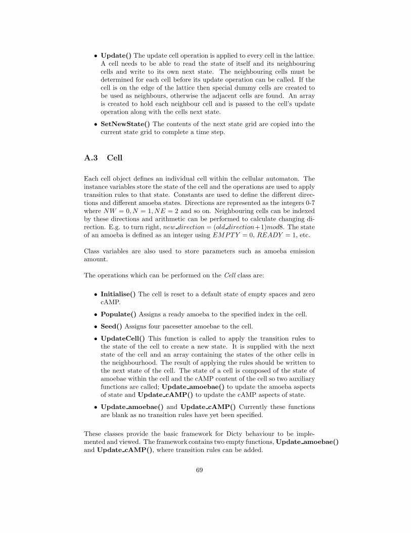
• Update() The update cell operation is applied to every cell in the lattice.A cell needs to be able to read the state of itself and its neighbouringcells and write to its own next state. The neighbouring cells must bedetermined for each cell before its update operation can be called. If thecell is on the edge of the lattice then special dummy cells are created tobe used as neighbours, otherwise the adjacent cells are found. An arrayis created to hold each neighbour cell and is passed to the cell’s updateoperation along with the cells next state.

• SetNewState() The contents of the next state grid are copied into thecurrent state grid to complete a time step.

A.3 Cell

Each cell object defines an individual cell within the cellular automaton. Theinstance variables store the state of the cell and the operations are used to applytransition rules to that state. Constants are used to define the different direc-tions and different amoeba states. Directions are represented as the integers 0-7where NW = 0, N = 1, NE = 2 and so on. Neighbouring cells can be indexedby these directions and arithmetic can be performed to calculate changing di-rection. E.g. to turn right, new direction = (old direction+1)mod8. The stateof an amoeba is defined as an integer using EMPTY = 0, READY = 1, etc.

Class variables are also used to store parameters such as amoeba emissionamount.

The operations which can be performed on the Cell class are:

• Initialise() The cell is reset to a default state of empty spaces and zerocAMP.

• Populate() Assigns a ready amoeba to the specified index in the cell.

• Seed() Assigns four pacesetter amoebae to the cell.

• UpdateCell() This function is called to apply the transition rules tothe state of the cell to create a new state. It is supplied with the nextstate of the cell and an array containing the states of the other cells inthe neighbourhood. The result of applying the rules should be written tothe next state of the cell. The state of a cell is composed of the state ofamoebae within the cell and the cAMP content of the cell so two auxiliaryfunctions are called; Update amoebae() to update the amoeba aspectsof state and Update cAMP() to update the cAMP aspects of state.

• Update amoebae() and Update cAMP() Currently these functionsare blank as no transition rules have yet been specified.

These classes provide the basic framework for Dicty behaviour to be imple-mented and viewed. The framework contains two empty functions, Update amoebae()and Update cAMP(), where transition rules can be added.

69