KTH Stockholm, 2017

A Case of Road Design in Mountainous Terrain with an

Evaluation of Heavy Vehicles Performance

Barbora Srnová

Master Thesis in Highway Engineering

Stockholm, June 2017

KTH Stockholm, 2017

i

KTH Stockholm, 2017

ii

Acknowledgements

This master thesis was carried out at the School of Civil Engineering at the Technical University of Madrid

(Universidad Politécnica de Madrid) under supervising of prof. Manuel G. Romana from UPM, Madrid and

Romain Balieu from KTH, Stockholm.

I would like to thank the Technical University of Madrid for allowing me to work on this thesis in their labs

and their computers throughout the whole duration of the thesis. It was a great experience to spend 5

months at UPM Madrid alongside PhD students who also helped and supported me.

I would also like to thank KTH Stockholm for their support while I was reaching out to UPM Madrid and

during my stay there. I appreciate their help throughout this project and throughout my whole master

degree studies at KTH Stockholm.

My thanks goes also to Ricardo Lorenzale Grande from UPM Madrid, who patiently helped me with

learning how to work with software Tool CLIP and always promptly answered my questions.

Last but not least, I want to emphasize the support that my parents and family have provided me with, I

would never be able to chase my dreams and ambition without their continuous help and encouragement

for what I am incredibly grateful.

Stockholm, June 2017

Barbora Srnová

KTH Stockholm, 2017

iii

KTH Stockholm, 2017

iv

Abstract

Traffic situation in the mountainous surroundings of Navas del Rey, Spain, requires a new solution to

improve the road M-501 leading long way around the town. In this project, a solution was suggested and

analyzed. A new road was designed to make the path shorter and more convenient for drivers passing the

area every day.

The new road was selected from three alternatives and detailed design was presented in this project. The

road provides smooth drive through horizontal and vertical alignments with a short section of steep

longitudinal grade. This can cause difficulties especially to heavy vehicles, which were thereafter analyzed.

The heavy vehicles performance is affected by several factors, including longitudinal grade, horizontal

curve radii and vehicle characteristics. Number of different solutions were presented and described.

Eventually, the most suitable option for the new road was selected. For the section with steep longitudinal

grade, 2+1 roadway will be applied to increase capacity of the road. Time period restrains will also be

installed to eliminate heavy vehicles from passing the new road during peak hours on working days.

Key words: road design, steep grade, upgrade, downgrade, heavy vehicles, passenger car equivalent,

mountainous terrain

KTH Stockholm, 2017

v

KTH Stockholm, 2017

vi

Notation

Abbreviations:

AASHTO American Association of State Highway and Transportation Officials

ADT Average Daily Traffic

AV Autonomous Vehicles

EU European Union

EUR Euro, Currency of Eurozone

HCM Highway Capacity Manual

LOS Level of Service

NMAS Nominal Maximum Aggregate Size

PCE Passenger Car Equivalent

SEK Swedish crown, Swedish currency

UPM Universidad Politécnica de Madrid (Technical University of Madrid)

WTPR Weight-to-Power Ratio, kg/kW

Symbols:

a deceleration rate, m/s2

L minimum length of spiral, m

R radius of curve measured to a vehicles’ center of gravity, m

Rmin minimum radius of curve, m

s grade of an uphill/downhill, %

V design speed, km/h

v vehicle speed, m/s

v/c volume-to-capacity ratio

y elevation for the parabola, m

KTH Stockholm, 2017

vii

KTH Stockholm, 2017

viii

Table of Contents List of Figures ................................................................................................................................................ x

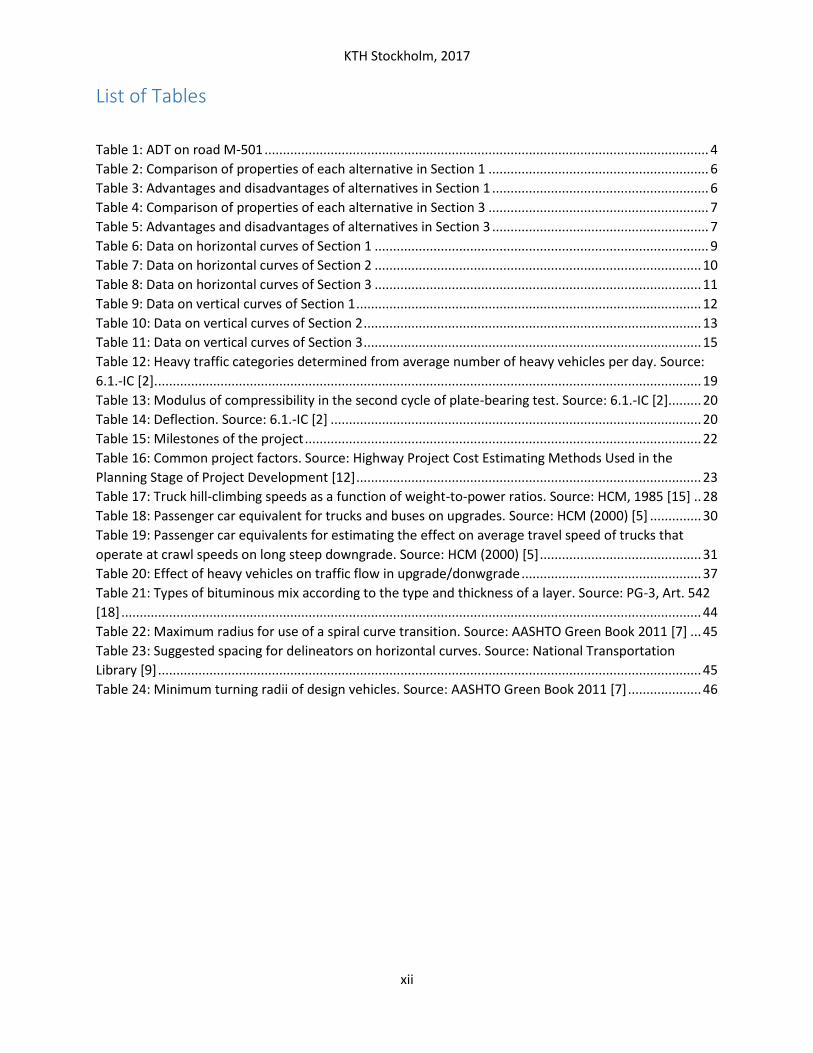
List of Tables ............................................................................................................................................... xii

1 Introduction .......................................................................................................................................... 1

2 Road design ........................................................................................................................................... 3

2.1 Introduction .................................................................................................................................. 3

2.2 Methodology ................................................................................................................................. 5

2.2.1 Software ................................................................................................................................ 5

2.2.2 Alternatives ........................................................................................................................... 5

2.2.3 Horizontal alignment ............................................................................................................. 8

2.2.3.1 Section 1 ............................................................................................................................ 9

2.2.3.2 Section 2 ............................................................................................................................ 9

2.2.3.3 Section 3 .......................................................................................................................... 10

2.2.4 Vertical alignment ............................................................................................................... 11

2.2.4.1 Section 1 .......................................................................................................................... 11

2.2.4.2 Section 2 .......................................................................................................................... 13

2.2.4.3 Section 3 .......................................................................................................................... 14

2.2.5 Cross Section ....................................................................................................................... 16

2.2.6 Road structure and materials .............................................................................................. 19

2.2.7 Schedule .............................................................................................................................. 21

2.2.8 Cost estimation ................................................................................................................... 22

2.3 Results and Discussion................................................................................................................. 25

3 Heavy vehicles performance ............................................................................................................... 27

3.1 Introduction ................................................................................................................................ 27

3.2 Methodology ............................................................................................................................... 28

3.2.1 Passenger Car Equivalent .................................................................................................... 28

3.2.2 Geometric design ................................................................................................................ 31

3.2.3 Traffic adjustments .............................................................................................................. 34

3.3 Results and Discussion ................................................................................................................ 35

4 Suggestions for further work .............................................................................................................. 39

References .................................................................................................................................................. 41

Appendix A: Figures and Tables .................................................................................................................. 43

Appendix B: Cost Estimation ....................................................................................................................... 48

Appendix C: Drawings ................................................................................................................................. 50

KTH Stockholm, 2017

ix

KTH Stockholm, 2017

x

List of Figures

Figure 1: Location of Navas del Rey in Spain ................................................................................................ 3

Figure 2: Location of Navas del Rey in Community of Madrid ..................................................................... 3

Figure 3: Existing road M-501 in grey color .................................................................................................. 4

Figure 4: ADT on road M-501 ........................................................................................................................ 4

Figure 5: Alternatives for Section 1 ............................................................................................................... 6

Figure 6: Alternatives for Section 3 ............................................................................................................... 7

Figure 7: Existing road M-501 in grey color, new road in red color.............................................................. 8

Figure 8: Sections 1-3 of the new road ......................................................................................................... 8

Figure 9: Mass diagram of Section 1 ........................................................................................................... 12

Figure 10: Haul of Section 1 ........................................................................................................................ 13

Figure 11: Mass diagram of Section 2 ......................................................................................................... 14

Figure 12: Haul of Section 2 ........................................................................................................................ 14

Figure 13: Mass diagram of Section 3 ......................................................................................................... 15

Figure 14: Haul of Section 3 ........................................................................................................................ 16

Figure 15: Example cross-section in tangent. Captured from drawing no. 25 ........................................... 17

Figure 16: Concrete safety barrier (Photo Illustration). Source: smithmidland.com ................................. 18

Figure 17: Delineator posts (Photo Illustration). Source: globalsources.com ............................................ 19

Figure 18: Pavement structure. Captured from drawing no. 25................................................................. 20

Figure 19: Speed-distance curves for a typical heavy truck of 120 kg/kW for deceleration on upgrades.

Source: HCM 2000 [5] ................................................................................................................................. 32

Figure 20: Example of a climbing lane on two-lane highway. Source: AASHTO Green Book 2011 [7] ....... 32

Figure 21: Schematic of 2+1 roadway. Source: AASHTO Green Book 2011 [7] .......................................... 33

Figure 22: Passing lanes section on two-lane roads. Source: AASHTO Green Book 2011 [7] .................... 33

Figure 23: Illustration of the elevation and longitudinal grade of the entire road..................................... 35

Figure 24: Speed of trucks driving from the reading station 6.9 km to 0.0 km .......................................... 35

Figure 25: Travel time for trucks driving from the reading station 6.9 km to 0.0 km ................................ 36

Figure 26: Goods transport by mode in EU (2009). Source: European Road Statistics (2011) [1] ............. 43

Figure 27: Passenger transport modal split in EU (2009). Source: European Road Statistics (2011) [1] .... 43

Figure 28: Catalogue of pavement structures for heavy vehicle traffic categories T00 to T2. Source: 6.1.-

ID [2] ............................................................................................................................................................ 44

Figure 29: Speed-distance curves for a heavy truck of 85 kg/kW for deceleration on upgrades. Source:

3.1-IC (1999) ................................................................................................................................................ 47

KTH Stockholm, 2017

xi

KTH Stockholm, 2017

xii

List of Tables

Table 1: ADT on road M-501 ......................................................................................................................... 4

Table 2: Comparison of properties of each alternative in Section 1 ............................................................ 6

Table 3: Advantages and disadvantages of alternatives in Section 1 ........................................................... 6

Table 4: Comparison of properties of each alternative in Section 3 ............................................................ 7

Table 5: Advantages and disadvantages of alternatives in Section 3 ........................................................... 7

Table 6: Data on horizontal curves of Section 1 ........................................................................................... 9

Table 7: Data on horizontal curves of Section 2 ......................................................................................... 10

Table 8: Data on horizontal curves of Section 3 ......................................................................................... 11

Table 9: Data on vertical curves of Section 1 .............................................................................................. 12

Table 10: Data on vertical curves of Section 2 ............................................................................................ 13

Table 11: Data on vertical curves of Section 3 ............................................................................................ 15

Table 12: Heavy traffic categories determined from average number of heavy vehicles per day. Source:

6.1.-IC [2]. .................................................................................................................................................... 19

Table 13: Modulus of compressibility in the second cycle of plate-bearing test. Source: 6.1.-IC [2] ......... 20

Table 14: Deflection. Source: 6.1.-IC [2] ..................................................................................................... 20

Table 15: Milestones of the project ............................................................................................................ 22

Table 16: Common project factors. Source: Highway Project Cost Estimating Methods Used in the

Planning Stage of Project Development [12] .............................................................................................. 23

Table 17: Truck hill-climbing speeds as a function of weight-to-power ratios. Source: HCM, 1985 [15] .. 28

Table 18: Passenger car equivalent for trucks and buses on upgrades. Source: HCM (2000) [5] .............. 30

Table 19: Passenger car equivalents for estimating the effect on average travel speed of trucks that

operate at crawl speeds on long steep downgrade. Source: HCM (2000) [5] ............................................ 31

Table 20: Effect of heavy vehicles on traffic flow in upgrade/donwgrade ................................................. 37

Table 21: Types of bituminous mix according to the type and thickness of a layer. Source: PG-3, Art. 542

[18] .............................................................................................................................................................. 44

Table 22: Maximum radius for use of a spiral curve transition. Source: AASHTO Green Book 2011 [7] ... 45

Table 23: Suggested spacing for delineators on horizontal curves. Source: National Transportation

Library [9] .................................................................................................................................................... 45

Table 24: Minimum turning radii of design vehicles. Source: AASHTO Green Book 2011 [7] .................... 46

KTH Stockholm, 2017

xiii

KTH Stockholm, 2017

1

1 Introduction

Road infrastructure is essential part of infrastructure services provided to the society among

other technical structures, such as railways, bridges, tunnels, water supply, electric grids,

telecommunications, etc. Road transport stands for most of the passenger and goods transport in

European Union according to the European Road Statistics [1] from 2011. Goods transport in

European Union consists from the road transport of up to 47% (2009), while passenger transport

on roads is up to 74% of all transport modes (2009) [1].

Therefore, it has been of great importance to build and improve high-quality road systems in

order to accommodate the needs of society. By combination of well-designed traffic system,

proper road structure and geometric design, the optimal highway can be built. Improvements in

road systems are achieved in various sectors of the road design, such as safer intersections, more

durable road pavements, better understanding of vehicles performance, etc.

This project will address two closely related topics: solution of a traffic difficulty in Navas del

Rey area in Community of Madrid, Spain, and evaluation of heavy vehicles performance in

mountainous terrains. While the first part of the thesis will be focused on design of a new road as

a solution of exasperating traffic situation in Navas del Rey, containing geometric design, road

structure design, budget and schedule, the second part of the thesis will answer and elaborate on

couple questions arising from the design part.

Aim of this project is to solve various issues in traffic engineering by using means of civil

engineering knowledge and experiences. The first major issue to be solved is the existent path of

road M-501 which leads a long way around the town of Navas del Rey, as will be shown later. This

path will be changed into a shorter one making it easier and faster to pass the inconvenient section

of the road. However, design of this road will form new questions and issues to be solved, out of

which the most important one will be addressed, because one part of the newly designed road will

have a 9% grade for more than 1.5 km, and performance of heavy vehicles in such conditions

creates significant difficulties in traffic. This behavior will be studied and possible solutions

suggested.

Road design in Spain is carried out according to Spanish design guidelines and standards, which

are Instrucción de Carreteras and Pliego de Prescripciones Técnicas Generales para obras de

carreteras y puentes (PG-3). These set of standards and technical aspects were developed by

Ministerio de Formento (Ministry of Public Works) and they are the only standards in Spain that

are required to be followed. Sections of Instrucción de carreteras interesting for this project are:

Norma 3.1.–IC. Trazado de carreteras (Geometric design of roads)

Norma 5.2.–IC. Drenaje superficial (Surface drainage)

Norma 6.1.–IC. Secciones de firme (Pavement for new roads) [2]

Norma 8.1.-IC. Señalización vertical (Vertical signing)

The standard PG-3 provides specifications for road construction – for basic materials and final

elements of the road.

KTH Stockholm, 2017

2

Because these standards are published only in Spanish language, translation to English would

take too much time, therefore this project was designed according to American standards AASHTO

- A Policy on Geometric Design of Highways and Streets (AASHTO Green Book) and Highway Capacity

Manual (HCM). In the United States of America, it is required to follow these standards for a road

design. Even though some of the data presented in AASHTO Green Book and HCM differ from data

in IC and PG-3 due to slightly different dimensions of vehicles in USA and Europe, most of the

guidelines are the same for American and Spanish standards.

KTH Stockholm, 2017

3

2 Road design

2.1 Introduction Navas del Rey is a town in the Community of Madrid, located 52 km west from the

capital of Spain, Madrid. The town is accessed by the road M-501, adjustment of which will be

the object of this project. The town is surrounded by village Robledo de Chavela and towns

Chapinería and Colmenar from the north and east. To the south of Navas del Rey is Aldea del

Fresno, and in the southwest, there is Pelayos Dam separated from the town by a mountain.

Figure 1: Location of Navas del Rey in Spain

Figure 2: Location of Navas del Rey in Community of Madrid

The existing road M-501 begins at the intersection of M-40 and M-511 in Madrid as

four-lane motorway and continues as such for 48 km until it reaches the town of Navas del

Rey. At this point, the road is narrowed to two lanes and continues north through the town to

pass around the mountain. Eventually it turns to southwest again and crosses the Pelayos Dam

to continue further southwest. This path of two-lane road is shown in Figure 3 and is of interest

in this project.

KTH Stockholm, 2017

4

Figure 3: Existing road M-501 in grey color

The section highlighted in grey color in the figure above is 9.4 km long with Average

Daily Traffic ADT = 12 893 veh/day, out of which 7.25% is heavy vehicles (2015) [3]. ADT in this

section of road M-501 has had an increasing tendency in recent years, as can be seen in Figure

4 and Table 1. Therefore, the importance of improving the traffic and travel conditions in this

area is increasing too.

Figure 4: ADT on road M-501

2011 2012 2013 2014 2015

10 900 10 900 10 900 11 930 12 893 Table 1: ADT on road M-501

The main problem to be addressed is the detour that drivers have to take in order to

get from Navas del Rey to the Pelayos Dam, the direct distance is approximately 4 km shorter

(L = 5.6 km) than the existing path. The aim of this project is to design a new path of the road

M-501 in a way that the traveling distance and time will decrease while improving the capacity

of the road. Also, traffic safety and comfort will be considered in the design.

9 000

10 000

11 000

12 000

13 000

14 000

2011 2012 2013 2014 2015

AD

T (v

eh/d

ay)

Year

ADT on road M-501

KTH Stockholm, 2017

5

2.2 Methodology

2.2.1 Software

Road design can be done in number of different software programs developed to make

an engineer’s life easier. Some countries and some institutions create their own program that

suits the best the conditions and standards of the country. Some of these software are:

AutoCAD Civil 3D (USA), Tool CLIP (Spain), Trimble Quantm (Australia), etc.

Geometric design in this project was done in Spanish software Tool CLIP, a 3D designing

program developed for design, evaluation and control of execution and construction of

highways and railways. This software was used because the designed road is located in Spain

and the input material needed for design was available only for work in CLIP.

The program CLIP provides a designer with infinite number of possibilities and options

to carry out a road design. It allows a user to freely create horizontal and vertical alignments,

adjusting any variables desired, including design velocity, width of the road, road cross slopes,

cut and fill slopes, thickness of road structure, etc. Once the horizontal and vertical alignments

are created, they are used by the software to create cross sections of the road. Eventually, the

software provides the designer with a 3D dynamic view useful for estimation whether the

horizontal and vertical curves are compatible. This is essential for road safety – stopping sight

distance and decision sight distance must be sufficient to prevent accidents.

2.2.2 Alternatives

Designing a road is a complicated process requiring evaluation of different alternatives

based on their horizontal and vertical alignment, the position within the area, budget, etc. This

kind of evaluating is important to make sure that the designed road will be safe, sufficient for

the traffic demand, economical and long-lasting. The alternatives can differ in everything from

radii of horizontal curves through road structure and material use to intersections.

The path of the road designed in this project is divided into 3 sections as will be

explained in detail later in this chapter. However, only two of these sections were evaluated

from several different alternatives. Section 2 (see Figure 8) was designed as reconstruction of

existing road, therefore its geometric design only followed the road in place. Section 1 and

Section 3 were designed as a new road with three alternatives each. These are presented in

Figure 5 and Figure 6. The most important factor for evaluation of different alternatives in this

project was horizontal and vertical alignment. Economical evaluation was carried out only for

the chosen path.

KTH Stockholm, 2017

6

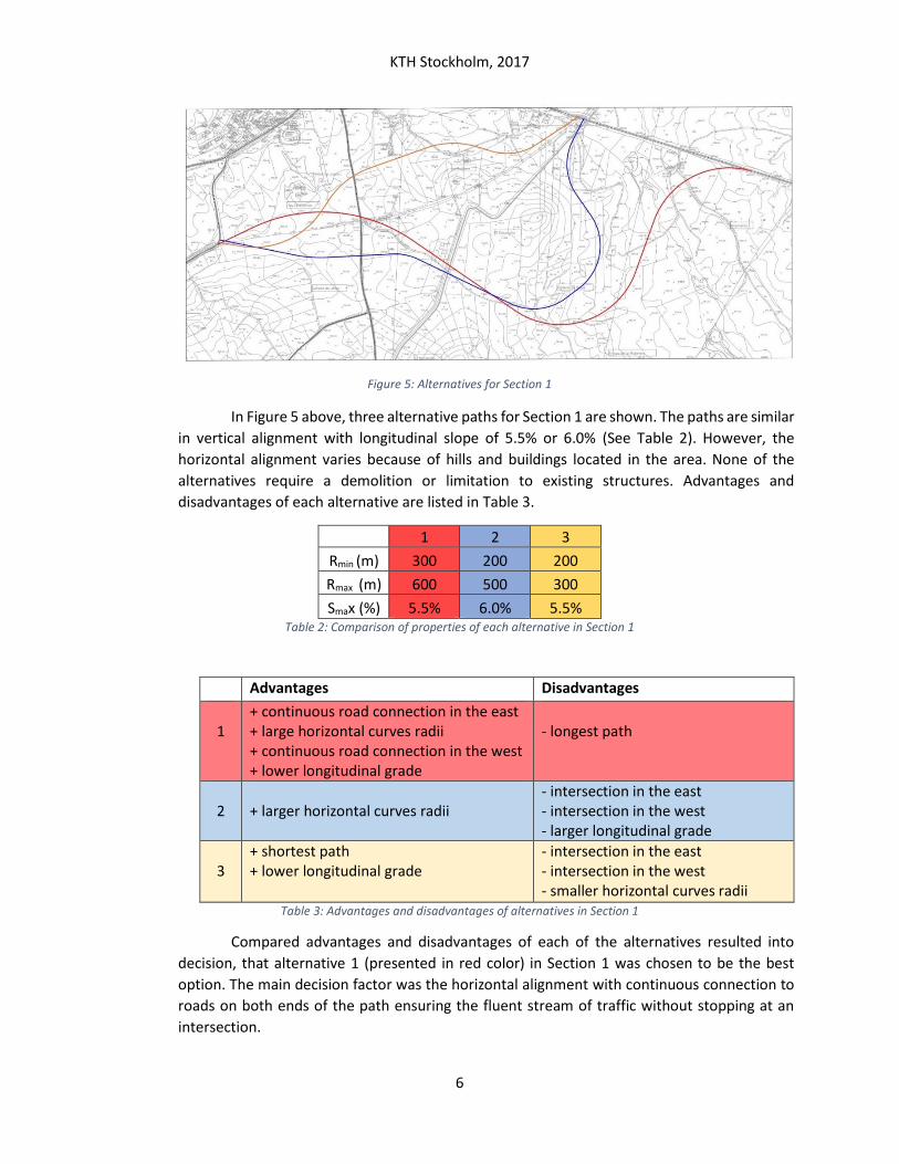
Figure 5: Alternatives for Section 1

In Figure 5 above, three alternative paths for Section 1 are shown. The paths are similar

in vertical alignment with longitudinal slope of 5.5% or 6.0% (See Table 2). However, the

horizontal alignment varies because of hills and buildings located in the area. None of the

alternatives require a demolition or limitation to existing structures. Advantages and

disadvantages of each alternative are listed in Table 3.

1 2 3

Rmin (m) 300 200 200

Rmax (m) 600 500 300

Smax (%) 5.5% 6.0% 5.5% Table 2: Comparison of properties of each alternative in Section 1

Advantages Disadvantages

1

+ continuous road connection in the east + large horizontal curves radii + continuous road connection in the west + lower longitudinal grade

- longest path

2

+ larger horizontal curves radii

- intersection in the east - intersection in the west - larger longitudinal grade

3

+ shortest path + lower longitudinal grade

- intersection in the east - intersection in the west - smaller horizontal curves radii

Table 3: Advantages and disadvantages of alternatives in Section 1

Compared advantages and disadvantages of each of the alternatives resulted into

decision, that alternative 1 (presented in red color) in Section 1 was chosen to be the best

option. The main decision factor was the horizontal alignment with continuous connection to

roads on both ends of the path ensuring the fluent stream of traffic without stopping at an

intersection.

KTH Stockholm, 2017

7

A path in Section 3 was also chosen from three different alternatives as is shown in

Figure 6. Path 1 (red) and path 2 (blue) are very similar in horizontal alignment with small

adjustments causing difference between their vertical alignment. In the meantime, the 3rd

alternative (orange) differs from the other two in horizontal alignment, and it also reaches a

longitudinal slope of 11%. More properties of each of the alternatives are shown in Table 4.

Figure 6: Alternatives for Section 3

1 2 3

Rmin (m) 100 100 55

Rmax (m) 300 300 600

Smax (%) 9.0% 10.0% 11.0% Table 4: Comparison of properties of each alternative in Section 3

Advantages and disadvantages of these alternatives are listed in Table 5 below. The most important factor in deciding which alternative would be the best was vertical alignment. Longitudinal slopes are large in all three paths due to overcoming a mountain which will negatively influence the traffic flow through the section. However, counter-measures can be taken to limit the influence. This will be further discussed later. The alternative with the lowest longitudinal grade was the path 1 (shown in red color), therefore this alternative was chosen to be the best one. An important factor which also contributed to this decision was the continuous transition from the newly designed road to the existing road in the west end of the path.

Advantages Disadvantages

1

+ lowest longitudinal grade + larger horizontal curves radii + continuous road connection in the west

- longest path

2

+ larger horizontal curves radii

- larger longitudinal grade

3

+ shortest path + large horizontal curve radius Rmax

- largest longitudinal grade - connects to an unpaved road in the west - small horizontal curves radii Rmin

Table 5: Advantages and disadvantages of alternatives in Section 3

KTH Stockholm, 2017

8

2.2.3 Horizontal alignment

The horizontal alignment of the new road was designed in the software Tool CLIP. The

initial input material to the program was a map of the area obtained from map and register

database at the UPM. The map contained contour lines, existing roads, buildings and water

areas. Based on this map, different horizontal alignment alternatives were suggested, out of

which one was chosen for detailed design (see 2.2.2). The choice was based on radii of curves

and continuity of the horizontal alignment as well as on vertical alignment.

Figure 7: Existing road M-501 in grey color, new road in red color

In the Figure 7 above, the situation of the area can be seen. The existing road M-501 is

shown in grey color and the new road is shown in red. The new road will start before the

existing road M-501 reaches the roundabout near Navas del Rey and will continue to the

southwest to the point, where it will connect to the existing M-501 before it reaches the

Pelayos Dam. The new road is 2.5 km shorter than the existing road, resulting in the length of

L = 6.9 km. The road is divided into 3 sections based on differing conditions influencing the

horizontal and vertical alignment, and material of the foundation. The three different sections

can be seen in the Figure 8. All three sections create a continuous road without a need of an

intersection. In points where the existing road M-501 connects with Section 1 in the East and

Section 3 in the West, intersections will be applied. However, the newly designed road will be

the main road and existing M-501 will yield.

Figure 8: Sections 1-3 of the new road

KTH Stockholm, 2017

9

2.2.3.1 Section 1

Section 1 of the new road is the eastern part of the road with reading station 0+000.00

at the east end of the section. This section is located in an area where no other roads occur,

therefore the horizontal alignment offered various possibilities for design. Section 1 smoothly

passes between two peaks and ends at the point, where it connects to the existing road leading

southwards. The horizontal alignment of Section 1 is 2.445 km long and consists of 3 curves of

different lengths and radii. The detailed data on the geometric properties of the curves can be

seen in Table 6. Design of transition curves is not necessary here, since Ri > 148 m (see Table 6

and Table 22). According to the Table 22, maximum curve radius when a transition curve is

necessary is Rmax = 148 m at design velocity V = 50 km/h. A drawing of horizontal alignment

and cross sections of Section 1 can be found in Appendix C: Drawings.

.

Table 6: Data on horizontal curves of Section 1

2.2.3.2 Section 2

Section 2 is 2.607 km long and the existing road is composed of two parts: short

segment of 0.6 km is paved road, while the rest 2.1 km of the section is unpaved local road.

The horizontal alignment of the new road mostly follows the existing unpaved road; however,

small adjustments were made near intersections. The Section 2 contains 8 curves, where Rmin

= 200.00 m and Rmax = 500.00 m, as seen in Table 7. Transition curves are not needed in this

section either, since the Rmin > 148 m (Table 22). A drawing of horizontal alignment and cross

sections of Section 2 can be found in Appendix C: Drawings.

Reading Station

Length (m) Radius (m)

0+181,44 76,51 500,00

0+257,95

0+477,89 167,47 200,00

0+645,36

0+696,74 91,06 200,00

0+787,80

0+970,63 76,80 200,00

1+047,43

1+144,04 173,75 500,00

1+317,79

Reading Station

Length (m) Radius (m)

0+017,39 432,91 300,00

0+450,29

0+653,77 548,23 300,00

1+202,00

1+671,42 630,20 600,00

2+301,61

KTH Stockholm, 2017

10

1+375,16 182,52 400,00

1+557,68

1+615,51 156,22 300,00

1+771,73

2+001,32 212,68 500,00

2+213,99 Table 7: Data on horizontal curves of Section 2

2.2.3.3 Section 3

The final section of the new road will start where the previous part of existing unpaved

road ends. This segment is very important for its large difference in altitude between the start

and the end point. Therefore, the horizontal curves are of small radii and in proximity to each

other. Section 3 also differs from the other two sections in its cross-section disposition.

Although the first two sections are a two-lane road, Section 3 is designed as a 2+1 road.

2+1 roadway is a concept that has been found to improve operational efficiency and

reduce crashes for selected two-lane highways [4]. The concept provides a three-lane cross

section by implementing passing lanes in alternating directions throughout the whole section

(see Figure 21). Areas with difficult conditions require additional passing lanes in order to

improve the capacity and comfort of the road. 2+1 roadway concept was designed in Section

3, because the vertical alignment introduced high grade percentage and therefore

deterioration in traffic fluency. This situation influences specifically performance of heavy

vehicles, which will be discussed in detail in Chapter 0.

The horizontal alignment of Section 3 is more complicated than of the previous

sections due to uneasy terrain. This part is 1.856 km long and contains 7 horizontal curves,

some of which create 2 S-curves, where the radius R = 100.00 m. Since R < 148 m (as explained

above), transition curves for these horizontal curves are needed to secure fluent transition

between a tangent and a curve. Length of transition curves was automatically calculated by

software CLIP. In the Table 8 below, geometric properties of horizontal alignment can be found.

A drawing of horizontal alignment and cross sections of Section 3 can be found in Appendix C:

Drawings.

Reading Station Length (m) Radius (m) Transition

Curve Parameter

0+390,95 126,00 300,00

0+516,95

0+631,19 109,92 200,00

0+741,11

0+743,86 42,25 65

0+786,11

0+786,11 62,62 100,00

0+848,73

0+848,73 42,25 65

KTH Stockholm, 2017

11

0+890,98

0+894,94 42,25 65

0+937,19

0+937,19 26,74 100,00

0,963,93

0+963,93 42,25 65

1+006,18

1+190,65 42,25 65

1+232,90

1+232,90 39,16 100,00

1+272,06

1+272,06 42,25 65

1+314,31

1+321,17 42,25 65

1+363,42

1+363,42 34,15 100,00

1+397,56

1+397,56 42,25 65

1+439,81

1+606,70 77,25 300,00

1+683,95 Table 8: Data on horizontal curves of Section 3

2.2.4 Vertical alignment

The vertical alignment of the new road was designed in the software Tool CLIP. It is

important to maintain constant operation and capacity throughout the road section. This is

also influenced by vertical alignment: the grade (%) of road, the vertical curves, stopping sight

distance, etc. The vertical alignment of the new road was designed to follow the terrain as

much as possible in order to lower excavated rock volume as well as to decrease the need for

fill material and to reach balance between cut and fill. The terrain where the new road will be

located is defined as mountainous terrain: “A combination of horizontal and vertical

alignments causing heavy vehicles to operate at crawl speeds for significant distances or at

frequent intervals” [5]. In such cases, it is difficult to control cubature - to manipulate the

vertical alignment in a way that the excavation material volume is in balance with embankment

volume. Important criterion to ensure road safety is to make sure that horizontal and vertical

alignments are compatible and that stopping sight distance is reached. This matter was

checked for all sections using 3D dynamic view in software CLIP.

2.2.4.1 Section 1

Vertical alignment of Section 1 of the new road was important for horizontal alignment

design since this section passes between two hills. The maximum longitudinal grade reached

5.5% throughout almost 600 m of length. The alignment consists of 4 vertical symmetrical

parabolic curves of different radii. Length of each curve and elevation for the parabola (y) was

KTH Stockholm, 2017

12

automatically calculated by the software CLIP. Detailed properties of the vertical alignment are

displayed in Table 9. The drawings of longitudinal cross section can be found in Appendix C:

Drawings.

Reading Station Elevation Slope (%) Length (m) Radius (m) y (m)

0+000,000 692,000 0 0 0,000

0+341,250 678,350 -4,0 275 5 000 1,891

0+790,903 685,095 1,5 280 7 000 1,400

1+390,000 718,045 5,5 425 -5 000 -4,516

2+047,500 698,320 -3,0 140 10 000 0,245

2+445,323 691,709 -1,6 0 0 0,000 Table 9: Data on vertical curves of Section 1

Vertical alignment also determines the rock volume needed to excavate or to place. It

is important to evaluate balance between cut and fill in order to be able to estimate the time

necessary for excavation and financial resources required for excavation and embankment. For

this purpose, a mass diagram was carried out. The mass diagram is a graphical representation

of the cumulative amount of earthwork moved along the centerline and distances over which

the materials are to be transported [6]. Mass diagram from Figure 9 is simplified and shows

the change of earthwork volume across the whole Section 1. Positive numbers represent

volume of excavated material while the negative numbers show the volume of embankment.

Figure 9: Mass diagram of Section 1

While the mass diagram represents amount of moving material at each cross section,

it does not provide clear information on the total volume of excavation or fill. This can be found

in a haul diagram. Haul is defined as the transportation of excavated material from its original

position to its final location in the work or other disposal area [6]. The haul of Section 1 (Figure

10) contains only positive figures of rock volumes and the haul at the end of the section is

KTH Stockholm, 2017

13

59 931.6 m3 of excavated material, which means that almost 60 thousand cubic meters of this

material will be transported to a storage area. The distance and the direction of transport of

the excavated rock was not necessary to calculate for this project.

Figure 10: Haul of Section 1

2.2.4.2 Section 2

Design of vertical alignment for Section 2 was based on achieving balance between cut

and fill and reducing large longitudinal grade since the path leads through a valley. It was

not possible to make large changes to horizontal alignment because this section is a

reconstruction of an existing unpaved road, therefore the adjustments in vertical design

were limited to manipulation of horizontal alignment.

The vertical alignment of this section contains 5 vertical symmetrical parabolic curves

of radii from 3 000 m to 5 000 m. The steepest part of the section is from 1.687 km to 2.161

km (474 m) with grade smax = 6.5%. The length of each curve and elevation for the parabola

(y) were automatically calculated by software CLIP. Detailed geometric properties of vertical

alignment for Section 2 are presented in Table 10 below. Drawings of the longitudinal cross

section can be found in Appendix C: Drawings.

Reading Station Elevation Slope (%) Length (m) Radius (m) y (m)

0+000,000 692,679 0 0 0,000

0+500,694 682,665 -2,0 250 5 000 1,562

0+831,250 692,582 3,0 255 -3 000 -2,709

1+686,810 645,526 -5,5 480 4 000 7,200

2+160,760 576,334 6,5 280 -4 000 -2,450

2+467,010 674,802 -0,5 150 5 000 0,563

2+606,940 678,301 2,5 0 0 0,000 Table 10: Data on vertical curves of Section 2

As an effort to minimize the cut and fill to reach balance between excavation and

embankment, minor adjustments to horizontal alignment of existing road were made. Through

0

10000

20000

30000

40000

50000

60000

70000

0,0 0,5 1,0 1,5 2,0 2,5

Ro

ck V

olu

me

(m3 )

Reading Station (km)

Haul

KTH Stockholm, 2017

14

the design of vertical geometry, it was possible to make a balanced mass diagram and haul.

The Mass Diagram (Figure 11) displays the amount of earthwork needed at each cross section,

where positive figures mean that excavation will take place and negative figures show need for

embankment.

Figure 11: Mass diagram of Section 2

Data from the mass diagram were further processed to find Haul (Figure 12) for Section

2. The final amount of rock volume after earthwork was performed along the whole section is

1180.0 m3, which means that most of the excavated material will be used for the embankment

in a different location of the section and only 1180.0 m3 will not be used and therefore

transported to a storage area outside of the construction site.

Figure 12: Haul of Section 2

2.2.4.3 Section 3

The vertical alignment design for Section 3 was the most important factor in selecting

the best alternative out of the three proposed alternatives in the beginning of this chapter (see

2.2.2). The new road in this section will overcome a large elevation difference – 160 m of height

-30000

-20000

-10000

0

10000

20000

30000

0,0 0,5 1,0 1,5 2,0 2,5 3,0

Ro

ck V

olu

me

(m3 )

Reading Station (km)

Haul

KTH Stockholm, 2017

15

over the length of 1.86 km. The aim of this design was to decrease the longitudinal grade in

order to avoid traffic complications, such as decrease in traffic-flow rate and safety. For a road

in mountainous terrain and a design speed of 50 km/h, maximum longitudinal grade is 12% [7].

The vertical alignment of Section 3 consists of 2 vertical symmetrical parabolic curves

with radius R = 20 000 m. The largest longitudinal grade in this section and in the entire

designed road occurs from 0.30 km to 1.55 km (L = 1.25 km) with smax = 9.0 %. The grade of this

size and length required special facility adjustments to improve the performance of vehicles

and increase the safety on the road. The cross-section of the Section 3 was changed from two-

lane road into 2+1 roadway, which will allow overtaking and therefore smoother traffic flow.

This issue was already mentioned in Horizontal alignment, section 2.2.3.3 and will be further

explained in Chapter 0. Detailed geometric properties of vertical alignment for Section 3 are

presented in Table 11. Drawings of longitudinal cross-section can be found in Appendix C:

Drawings.

Reading Station Elevation Slope (%) Length (m) Radius (m) y (m)

0+000,000 678,000 0 0 0,000

0+300,000 657,000 -7,00 400 -20 000 -1,000

1+550,000 544,500 -9,00 100 -20 000 0,063

1+855,566 518,527 -8,50 0 0 0,000

Table 11: Data on vertical curves of Section 3

The mountainous terrain in Section 3 was the reason for the design of steep grade

along the whole section and it made it very difficult to avoid large excavation and embankment

volumes, which are not desired. In fact, the amount of earthwork throughout this section is

enormous. The volumes of earthwork at each cross-section are displayed in Figure 13, where

positive figures represent the amount of excavations and negative figures show the

embankment volumes.

Figure 13: Mass diagram of Section 3

-10000

-5000

0

5000

10000

15000

0,0

0,1

0,1

0,2

0,2

0,3

0,4

0,4

0,5

0,5

0,6

0,7

0,7

0,8

0,8

0,9

1,0

1,0

1,1

1,1

1,2

1,3

1,3

1,4

1,4

1,5

1,6

1,6

1,7

1,7

1,8

Ro

ck V

olu

me

(m3)

Reading Station (km)

Section 3 - Mass Diagram

KTH Stockholm, 2017

16

While the mass diagram above shows only rock volume at each cross-section along the

whole section, haul of Section 3 is of bigger interest due to more complex data being provided.

The Haul diagram (Figure 14) represents total earthwork of Section 3 summed up to see, how

much rock will not be used in any other location of the section. The final amount of unused

rock volume after the all earthwork is finished, is 170 808.0 m3 of excavated material. Since

hauls in previous sections were also excavated rock, the material will be transported to a

storage area outside of the construction site where it will be reused for other construction

projects.

Figure 14: Haul of Section 3

As was mentioned before, the new designed road is located in mountainous terrain

with large and long gradient, resulting in complicated vertical alignment design. Even though

the grade of Section 1 and Section 2 did not exceed 6.5%, the grade of Section 3 did not reach

grade lower than 7.5% for 1.85 km. This situation formed large amounts of earthwork in each

of the sections and created a haul from the entire road of 231 919.6 m3 of unnecessary

excavated material. However, a total of 117 026 m3 of excavated material will be used for

construction of embankments. An Excel file called: “Mass Diagram + Hauls.xlsx” providing

detailed data of rock volumes can be found on attached CD-drive.

Note: Small inaccuracies may occur in elevation of land and pavement as a result of separate

design for each section.

2.2.5 Cross Section

Cross-section is a vertical section of the ground and roadway at right angles to the

centerline of the roadway, including all elements of a highway or street from right-of-way line

to right-of-way line [5]. Cross-sections are an essential part of design, as they illustrate the road

structure, cross-slope, drainage features, inclination of road-side slopes, elevation of

pavement, etc. It is a custom that analyzed cross-sections are spaced 20 or 25 m apart over the

whole length of designed road. In Spain, the distance of 20 m is a common practice, therefore

there are 40 drawings of 348 cross-sections in Appendix C: Drawings. These cross-sections were

0

20000

40000

60000

80000

100000

120000

140000

160000

180000

0,0 0,2 0,4 0,6 0,8 1,0 1,2 1,4 1,6 1,8 2,0

Ro

ck V

olu

me

(m3 )

Reading Station (km)

Haul

KTH Stockholm, 2017

17

not shown in longitudinal cross-sections as it was not necessary for this project, however, each

cross-section in the drawings is assigned with a corresponding reading station.

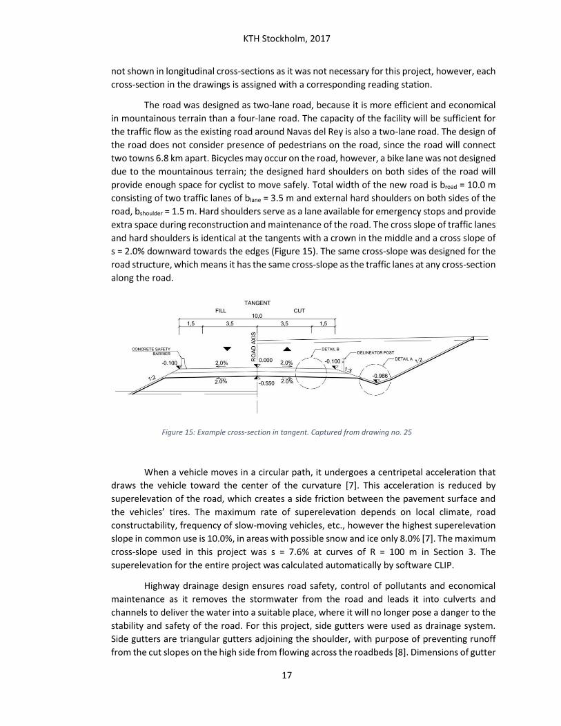
The road was designed as two-lane road, because it is more efficient and economical

in mountainous terrain than a four-lane road. The capacity of the facility will be sufficient for

the traffic flow as the existing road around Navas del Rey is also a two-lane road. The design of

the road does not consider presence of pedestrians on the road, since the road will connect

two towns 6.8 km apart. Bicycles may occur on the road, however, a bike lane was not designed

due to the mountainous terrain; the designed hard shoulders on both sides of the road will

provide enough space for cyclist to move safely. Total width of the new road is broad = 10.0 m

consisting of two traffic lanes of blane = 3.5 m and external hard shoulders on both sides of the

road, bshoulder = 1.5 m. Hard shoulders serve as a lane available for emergency stops and provide

extra space during reconstruction and maintenance of the road. The cross slope of traffic lanes

and hard shoulders is identical at the tangents with a crown in the middle and a cross slope of

s = 2.0% downward towards the edges (Figure 15). The same cross-slope was designed for the

road structure, which means it has the same cross-slope as the traffic lanes at any cross-section

along the road.

Figure 15: Example cross-section in tangent. Captured from drawing no. 25

When a vehicle moves in a circular path, it undergoes a centripetal acceleration that

draws the vehicle toward the center of the curvature [7]. This acceleration is reduced by

superelevation of the road, which creates a side friction between the pavement surface and

the vehicles’ tires. The maximum rate of superelevation depends on local climate, road

constructability, frequency of slow-moving vehicles, etc., however the highest superelevation

slope in common use is 10.0%, in areas with possible snow and ice only 8.0% [7]. The maximum

cross-slope used in this project was s = 7.6% at curves of R = 100 m in Section 3. The

superelevation for the entire project was calculated automatically by software CLIP.

Highway drainage design ensures road safety, control of pollutants and economical

maintenance as it removes the stormwater from the road and leads it into culverts and

channels to deliver the water into a suitable place, where it will no longer pose a danger to the

stability and safety of the road. For this project, side gutters were used as drainage system.

Side gutters are triangular gutters adjoining the shoulder, with purpose of preventing runoff

from the cut slopes on the high side from flowing across the roadbeds [8]. Dimensions of gutter

KTH Stockholm, 2017

18

standardly used in the USA following the Highway Design Manual may differ from the

dimensions used in Spain. The side gutter used in this project is a standard gutter with

dimensions: depth to the deepest point h = 0.15 m and width bgutter = 1.0 m. The gutter is

located at every cross-section which is constructed in cut, so the stormwater runs off the road

and does not stay by the road construction body which could cause undesired settlement of

the structure.

Sideslopes should be designed to enhance roadway stability and to provide a

reasonable opportunity for recovery for an out-of-control vehicle [7]. Foreslopes should not be

steeper than 1V:4H unless the road is located in an area that does not permit use of flatter

slopes. The backslopes should be 1V:3H or flatter, depending on the area requirements, space

availability, financial expenses and, most importantly, on stability of the slope. Because of the

design in a mountainous terrain, the foreslopes used in this project are 1V:3H, backslopes in

cut 1V:2H. In case of slope’s height H > 3.0 m, a backslope of 1V:1H were used. Backslopes in

fill were designed as 1V:2H, in case of height of slope H > 3.0 m, the slope of 1V:1.5H was

preferable. These sideslopes are acceptable in the area of Communidad de Madrid, where the

geological conditions are very convenient and suitable for construction in steeper slopes.

A roadside barrier is a longitudinal system used to shield motorists from obstacles or

slopes located along either side of a roadway [7]. In determining which type of a safety barriers

is the most appropriate, the height and slope of an embankment are the most important

factors. Rounding at the shoulder and at the toe of embankment slope can reduce the severity

of an accident and help the driver to keep vehicle control. The longitudinal safety barrier for

this project was designed only on the side of the fill in order to prevent vehicles from riding off

the road in sections with high embankment (see Figure 15). The barrier is placed on the outer

edge of the shoulder to leave the most

area of the hard shoulder free for

emergency stoppings and other

necessary operations. On the cut side of

the road, the foreslope is flat enough to

keep vehicles from serious crushes and

therefore no safety barrier is necessary.

The roadside barrier used in this project

is New Jersey wall (Figure 16) – a type of

concrete safety barrier New that can

provide strong support not only for

passenger cars, but also for heavy

vehicles.

Markings of the road systems provide road users with regulations, guidance or

warning, which is reason why markings are essential elements of driver communication.

Horizontal markings and vertical signs of the new road were not designed in this project as it

was not necessary for the purpose of the project. However, a requirement for all rural roads is

to install delineator posts to increase night visibility and visibility in rain and snow, when most

Figure 16: Concrete safety barrier (Photo Illustration). Source: smithmidland.com

KTH Stockholm, 2017

19

of the horizontal markings are covered and not visible. The

purpose of delineator post is to outline the edges of the

roadway and to accent critical locations. Delineators consist of

retroreflective devices which are able to reflect a vehicle light

from a distance of 300 m. The delineators in this project will

be mounted with posts 1.35 m above the pavement on the cut

side of the road, and installed without a post on the concrete

safety barrier, since the retroreflective elements should be

along the both sides of the road. The height of delineator posts

on concrete barriers is 0.45 m to ensure good visibility of

reflection. In the tangent sections, the delineators will be

spaced 150 m apart in a continuous line, placed 0.5 m outside

the hard shoulder [9]. The spacing of delineator posts in a

curve depends on radius of the curve, but should not be less than 6 m and more than 90 m.

The values for the spacing in curve can be seen in Table 23. The posts of delineators can be

made from various materials, such as: U-channel iron post, standard black pipe, plastic or

timber post. In this project, plastic delineator posts will be used, and because they are fragile,

they do not pose any risk for road safety.

2.2.6 Road structure and materials

Primary function of a road structure is to distribute applied vehicle loads to the sub-

grade and reduce them so they will not exceed bearing capacity of the sub-grade. Pavement

structure should provide a surface of desired quality, adequate skid resistance, favorable color

and light reflection and low noise pollution. A properly designed pavement ensures its

longevity, riding comfort and low maintenance cost.

Design of a road depends on the type of the road, average daily traffic, average daily

heavy vehicle traffic and geology of the subgrade. These factors decide whether the pavement

will be flexible or rigid, what thickness and material composition of the structure will be. These

design questions are answered in Spanish standard Norma 6.1.-IC dealing with pavement for

new roads.

Heavy traffic category of the road was determined from Table 12, where IMDp stands

for Average Daily Heavy Traffic and is expressed in heavy vehicles per day. As mentioned in 2.1,

the ADT on M-501 is 12 893 vehicle/day with 7.25% of heavy vehicles, which equals to 935

heavy vehicles per day. Therefore, the heavy traffic category is T1.

Table 12: Heavy traffic categories determined from average number of heavy vehicles per day. Source: 6.1.-IC [2].

Category of the subgrade (Categoria de explanada) is determined based on modulus

of compressibility from the second cycle of plate-bearing test performed according to the NLT-

Figure 17: Delineator posts (Photo Illustration). Source: globalsources.com

KTH Stockholm, 2017

20

357: Ensayo de carga con placa. The categories are E1, E2 and E3 (see Table 13). In this project,

the test was not performed neither the value calculated, therefore, the subgrade category E2

was assumed. For E2, the modulus of compressibility Ev2 = 120 MPa.

Table 13: Modulus of compressibility in the second cycle of plate-bearing test. Source: 6.1.-IC [2]

For the purpose of control of the subgrade execution and for the categories of heavy

traffic T00-T2, the maximum standard deflection is allowed in accordance with Table 14. The

shown values, however, are probable values of the support capacity of the subgrade, varying

due to changes in humidity. For the subgrade category E2, the maximum allowed deflection is

dmax = 200*10-2 mm.

Table 14: Deflection. Source: 6.1.-IC [2]

Based on heavy traffic category (T1) and subgrade category (E2), the thickness of the

pavement structure was designed according to the Figure 28. Structure number 122 was

selected consisting of 20 cm of hot bituminous mix (MB) as surface course and 25 cm of

stabilized cement (SC) as subbase. The subgrade of the pavement structure is 30 cm of

stabilized cement. The layers and the materials of the surface course were designed following

the Table 21. The pavement is displayed in Figure 18 and it is also included in the Appendix C:

Drawings, drawing No. 25.

Figure 18: Pavement structure. Captured from drawing no. 25

The function of surface course is to provide resistance against wear due to traffic loads,

to provide smooth riding surface for more comfort, to resist the vehicle pressure and surface

water infiltration. It also prevents horizontal shear stresses and vertical pressure produced by

moving or standing vehicle load and distributes the wheel load pressure [10]. The thickness of

the surface course is 20 cm and consists of the following layers:

KTH Stockholm, 2017

21

Semi-dense surface asphalt concrete with nominal maximum aggregate size of

16 mm, bitumen penetration index B40/50 and thickness t = 4 cm (AC 16 surf

S B40/50)

Semi-dense binder asphalt concrete with NMAS of 32 mm, B40/50, t = 6 cm

(AC 32 bin S B40/50)

Coarse base asphalt concrete with NMAS of 32 mm, B40/50, t = 10 cm (AC 32

base G B40/50)

The subbase course acts as support for surface course, it improves drainage condition

and protects upper layers from undesired qualities from underlying soils. The material used for

the subbase course is stabilized cement (SC) with thickness t = 25 cm.

Underneath the subbase course, subgrade layer is constructed, which receives the

distributed traffic load from the layers above, withstands all types of stresses imposed upon it

and acts as bedding layer for the whole structure.

2.2.7 Schedule

A schedule of construction project is important part of project documentation carried

out in order to establish production goals, to monitor and measure progress and to manage

changes to the project along the way. Time management of a project is essential to the entire

production, as it prevents and eventually solves issues of time delay or time conflict between

different activities.

Bar chart is the most commonly used method of planning and scheduling construction

projects [11]. Bar charts are easy to prepare, easily understood and they are oftentimes

referred to as Gantt charts. However, they do not show the relationships between activities

and what effect a time delay of one activity could have on the timeline of the rest of the project.

The position and length of each bar in the Gantt chart reflects how long each activity

is scheduled to last, when it starts and ends, what activities overlap and eventually, when the

entire project starts and ends. The excel file with schedule of this project can be found on

attached CD-drive as “Schedule.xlsx”.

Every construction project should have milestones which are important to reach

during the construction, because they provide easier check of completed project stages and

time delays. For this project, 13 milestones and expected time of their accomplishment have

been set:

Milestone Week

ML1 Access to all sites for surveying and geotechnical reconnaissance equipment to contractor 1

ML2 Approval of quality of surveying by client 4

ML3 Approval of quality and reliability of geotechnical knowledge by client 5

ML4 Approval of quality of Section 1 by client 11

ML5 Approval of quality of Section 3 by client 15

ML6 Approval of quality of Section 2 by client 18

KTH Stockholm, 2017

22

ML7 Approval of safety and adequacy of temporary facilities designed by client 19

ML8 Submittal of Draft Detailed Design to Client 20

ML9 Result of Review of Draft Detailed Design by Engineer 22

ML10 Result of Review of Draft Detailed Design by Client 23

ML11 Result of Review of Final Detailed Design by Engineer 28

ML12 Result of Review of Final Detailed Design by Client 31

ML13 Submittal of Final Detailed Design to Client 32 Table 15: Milestones of the project

The schedule of the construction project was divided into 9 groups of activities (A-I):

(A) Previous work, (B) Pre-construction activities, (C) Construction site preparation, (D) Section

1, (E) Section 2, (F) Section 3, (G) Translation and checking, (H) Final edition and submittal (Draft

Detailed) and (I) Final edition and submittal (Final Design). Each of these groups lasts from 5

weeks to 18 weeks, resulting in the scheduled length of the entire project to be 32 weeks (8

months).

Section 1 and Section 3 will start one week apart, Section 1 will start from the beginning

of the reading station, Section 3 from the end of the reading station and the construction will

continue towards the middle of the new road. This way, the works will be in progress in two

places at once, and the project completion time will be approximately 10 weeks shorter (the

time of construction of Section 3). Construction of Section 2 will start once Section 1 is finished,

and since it is scheduled that Section 2 activities finish after Section 3 is ready, the work of

these two parts will meet towards the end of reading station of Section 2.

The final 32 weeks of construction project consist of 17 weeks of construction work

and 15 weeks of administration work including planning, surveying, geotechnical study,

revisions and reviews, legislation check and final submittal.

2.2.8 Cost estimation

A road project like this one requires a cost estimation of the construction process. Cost

estimation is the process by which, based on information available at a particular phase of

project development, the ultimate cost of a project is estimated [12]. It is also the first estimate

used for evaluating budget and allocation of resources. Cost estimation is a part of the initial

project documentation that can help a project manager to make better decisions regarding the

limitations of the project.

A construction project is described by many factors, such as terrain, number of lanes,

rural or urban setting. Table 16 contains a list of factors typically used for estimation cost during

planning stage of the project. Most of these factors are considered in the cost estimation

carried out in this project. The cost estimation is provided in Appendix B: Cost Estimation. The

costs are divided into chapters in the attached cost estimation and these are: excavation,

transverse drainage, longitudinal drainage, pavement, signalization, environmental

integration, various, contingencies, safety and health at work, unknown and taxes.

KTH Stockholm, 2017

23

Cost of excavation accounts for excavation of top soil (t = 0.2 m) and mechanic

excavation of all the required soil as well as embankment works, including transport of the

material within the construction site or to a quarry. The amount of excavated material was

calculated from mass diagrams presented in 2.2.4.

Table 16: Common project factors. Source: Highway Project Cost Estimating Methods Used in the Planning Stage of Project Development [12]

Transverse drainage in this project are culverts for draining water away from the road

structure. The culverts are located every 50 m of the road and in the lowest points of the

vertical alignment to avoid standing water in sag. The number of culverts was assumed based

on this standard, but due to time restraints of the design work, they are not presented in

horizontal or vertical alignment drawings.

Longitudinal drainage will be installed on the cut sides of the road so the stormwater

from the road and slopes does not stay by the road but flows away and to a culvert. If the water

is not lead away from the road, it would significantly affect the material properties of the road

structure. Three types of longitudinal drainage are used: a side ditch covered with concrete

suitable for sections with longitudinal grade less than 1% or more than 3%; prefabricated ditch

appropriate for road sections where the sideslope exceeds height of 5.0 m; and concrete ditch

installed on the cut sides of the road where the two previous drainage types do not apply.

The cost of pavement was calculated separately for each material used considering the

thickness of a layer, width and length of the entire road. The pavement structure was explained

earlier in section 2.2.6. For the cost estimation, also 30 cm layer of subgrade was counted in as

a quality base for the road structure.

The price of horizontal and vertical signalization is estimated per kilometer of road and

represents only assumption of amount of used signalization. The exact number of vertical signs

or volume of horizontal signs was not calculated in this project.

Important part of every road project is environmental integration evaluating the

impact that the construction of the road has on the environment. Maintenance of the road

slopes to minimize the negative impact is a common practice to prolong the life of the entire

road structure. The cost estimation of environmental integration in this project includes:

unpacking of the land; maintenance, transport and spread of top soil from the excavation;

hydroseeding and maintenance of plant species. These values were assumed.

KTH Stockholm, 2017

24

From the chapter Various, the only process performed in this project is removing of

existing way in the Section 2. The length of the existing road is 600 m and it will be replaced

with a new road to match other sections of the road.

Cost estimates not always include contingencies – money added to the final cost

estimate as a precaution for unforeseen situations, such as weather delays or changes in scope

[12]. Depending on the size and difficulty of the project, contingencies add to a cost between

5% and 15%. For this project, 10% of the final cost was assumed.

Safety and health at work includes cost for introducing safety programs at the

construction site and for possible work-related injuries and illness. It is of utmost priority to

create a safe and healthy environment on the job site, therefore the cost of such precautions

is included in the initial estimation cost. For this project, 2% of final cost was assumed.

The cost estimation Chapter 10: Unknown assumes cost of some items not included in

the previous chapters due to the size of this project and the time constraints for submittal.

Items not included were, for instance: concrete barriers, delineator posts, management

overhead, etc. For these items, 15% of the final cost was assumed.

After all the chapters and items were put into cost estimation of the project and

summed up, the estimated cost was approximately 5.66 mil €. However, taxes apply for a

project cost. In Spain, the taxes for construction projects are 21%, which puts additional

1.19 mil € to the project cost resulting in the total estimated cost of 6.85 mil €.

The most costly item on the cost estimation list is hot bituminous mix with asphalt

binder resulting in up to 30% of the cost. The second most expensive item is excavation which

creates up to 24% of the cost. Such large number of resources will be used on earthwork

because the road is located in a mountainous terrain. The prices used in this project are

standard prices generally used in Madrid area, Spain in 2016.

KTH Stockholm, 2017

25

2.3 Results and Discussion

The goal of the project was to design a new road in order to improve traffic situation in

town Navas del Rey, Spain. The existing road M-501 leads a long way around Navas del Rey

to the Pelayos Dam because of the mountainous terrain surrounding the local towns.

Therefore, search for solution lead towards the project design of a new road that would

shorten the way between Navas del Rey and Pelayos Dam.

Initially, three alternatives of the road were designed with varying length and horizontal

and vertical alignment. After weighing advantages against disadvantages of each alternative,

the most suitable alternative was chosen and designed in detail. The length of the entire new

road passing through the mountainous terrain is 6.9 km, which is 2.5 km shorter than the

existing road M-501.

The vertical alignment significantly differs between the sections of the road – while the

maximum longitudinal grade in either of Section 1 or Section 2 is 6.5 %, it does not reach

lower value than 7.0 % at Section 3. This size of the longitudinal grade is allowed on rural

mountainous roads, however, it is inconvenient for mixed traffic including heavy vehicles. For

this reason, 2+1 roadway was designed in the Section 3.

The pavement structure was determined based on heavy vehicle traffic and environment

of the road surroundings. The thickness of the structure is 45 cm containing three layers of

different types of asphalt concrete (bituminous mix) at the surface, and different types of

stabilized cement as subbase and subgrade.

The schedule of the project in construction was assumed to be 32 weeks, accounting for

pre-work activities (planning, surveying), construction works (excavation, embankment,

pavement) and review and submittal activities. However, cost estimation was accounting

only for the construction works, such as excavation, embankment, pavement, drainage,

environment maintenance, etc. The estimated cost of the project is 6.85 mil €, tax included.

In this project, design of the new road will provide shorter path than the existing road,

through which the traffic situation around Navas del Rey will improve. However, this can be

said with certainty only for passenger cars and light vehicles, because heavy vehicles can

experience problems with steep longitudinal grade in Section 3. This issue will be further

discussed and solution suggested in the next chapter: Heavy vehicles performance.

KTH Stockholm, 2017

26

KTH Stockholm, 2017

27

3 Heavy vehicles performance

3.1 Introduction Road system is essential mean of passenger transport in Europe creating up to 74% (2009)

of all modes of transport (Figure 27). Goods transport also depends on a road transport, since

nearly 47% of all goods transport in Europe uses road system (Figure 26). This being said, heavy

vehicles play an important role in transport of goods and passengers, as trucks and buses can

carry heavy loads of cargo and large number of people.

Since heavy vehicles operate in the same traffic flow as passenger cars, bicycles and

pedestrians, it is necessary that the road design counts on all aspects of different behaviors.

Trucks and buses negatively influence the traffic operations and, possibly, capacity of facilities

due to their lower performance. The heavy weight being transported applies large load on the

road structure which deteriorates over time. However, heavy vehicles are necessary for well-

being of the society, hence new solutions must be developed in order to limit the negative

effect of heavy vehicles on the road structure and traffic flow.

The road M-501, which is of interest in this project, is a regional road connecting towns

across west part of Madrid region. The average daily traffic is ADT = 12 893 veh/day, out of

which 7.25% are heavy vehicles (see 2.1). Therefore, it is important to take heavy vehicles into

account in the design of the new road and consider their performance in all possible situations

to improve overall efficiency of the traffic operations.

3.1.1 Aim and objectives

In Chapter 2, design of new road M-501 was presented with detailed drawings and

explanation of used procedures. The new road was separated into three sections for easier

handling of varying data and properties of the landscape area. While Section 1 and Section 2

did not pose any issue in design, Section 3 formed a problem with its vertical alignment. Due

to a large elevation difference between the start and the end point of the section (160 m on

length of 1.86 km), the minimum value of longitudinal grade is smin = 7.0%, while the maximum

value is smax = 9.0% over 1.2 km of length. A longitudinal grade of this size causes decline of

traffic fluency and safety, therefore the aim of this chapter will be to find solution for

improvement of heavy vehicles performance in steep uphill/downhill and to reduce their

negative influence on traffic.

KTH Stockholm, 2017

28

3.2 Methodology

Performance of heavy vehicles on steep uphill/downhill has been studied by researchers

and vehicle producers for decades to find an optimal solution for improvement of heavy

vehicles performance in traffic. Many scientific articles and works have been published

focusing on explaining and reducing this issue. Solving the problem of negative influence of

heavy vehicles on traffic operations offers number of procedures to improve the situation.

3.2.1 Passenger Car Equivalent

The term Passenger Car Equivalent (PCE) was for the first time introduced in Highway

Capacity Manual 1965 to define the effect of trucks and buses in the traffic stream. It was

defined as “the number of passenger cars displaced in the traffic flow by a truck or a bus, under

the prevailing roadway and traffic conditions” [13]. This definition has evolved over the

decades of research and the most recent definition is from Highway Capacity Manual 2000 and

it is defined as “the number of passenger cars that are displaced by a single heavy vehicle of a

particular type under prevailing roadway, traffic and control conditions” [5]. In other words,

the Passenger Car Equivalent (PCE) represents the number of passenger cars that would

consume the same percentage of the highway’s capacity as the considered vehicle under

prevailing roadway, traffic and control conditions.

Passenger Car Equivalent (PCE) is a pre-design metric used to evaluate traffic-flow rate

on a road. PCE essentially represents the impact that a certain mode of transport has on traffic

variables (headway, speed, density) compared to a single passenger car. Since heavy vehicles

are larger than cars, typically have less acceleration and require more room for maneuvering

and braking, they cause a decrease in highway capacity. This impact on capacity is accounted

for by applying PCE value according to type of vehicle and facility [14]. PCE value of a heavy

vehicle depends on its weight, length, power and other characteristics, and also on number of

lanes of a road, speed, length and grade of an uphill. Converting heavy vehicles to equivalent

passenger cars is especially important when analyzing sections of highway with grades. The

influence of grade on performance of different types of trucks is shown in Table 17 as a

relationship between the grade, weight-to-power ratio (WTPR) and speed.

Percent Grade

Truck Hill-Climbing Speed (km/h)

60 kg/kW 120 kg/kW 180 kg/kW

3% 82 60 45

5% 71 42 31

7% 58 32 23 Table 17: Truck hill-climbing speeds as a function of weight-to-power ratios. Source:

HCM, 1985 [15]

As already mentioned, the PCE value depends on many factors, such as vehicle type, its dimensions, power, speed, acceleration and braking characteristics, but also road characteristics including gradients, curves, type of road (rural or urban) and presence and type

KTH Stockholm, 2017

29

of intersection [13]. Based on the importance of these variables in various road design projects dealing with different conditions, several methods of PCE calculation exist. Some of them are:

PCEs based on flow rates and density

PCEs based on headways

PCEs based on queue discharge flow

PCEs based on speed

PCEs based on delays

PCEs based on V/C ratio

PCEs based on vehicle-hour

PCEs based on travel time

PCEs based on HCM method

Most of these methods are focused on evaluation of PCE in urban areas, mainly at

intersections and congested areas, determining queue discharge flow, delays, volume-to-

capacity (v/c) ratio and vehicle-hours. Design of an urban road based on these parameters will

provide a good road, including suitable intersection and a traffic control. However, it is

important to realize that analysis of a rural road capacity is essential to ensure that the traffic

flow will be fully accommodated on the designed road with desired level of service (LOS). There

are two methods appropriate to use in the evaluation of the road in this thesis: PCEs based on

flow rates and density, and PCEs based on HCM method.

PCEs based on flow rates and density depend on the percentage of grade, mixed

vehicle flow and truck volume to capacity ratio [13]:

𝑃𝐶𝐸 = 𝑞𝐵 − 𝑞𝑀(1 − 𝑃𝑇)

𝑞𝑀 ∗ 𝑃𝑇

Where, qB = equivalent passenger car only flow rate for a given v/c ratio,

qM = mixed flow rate

PT = truck proportion in the mixed flow.

The variables in this equation can be found in annual reports by authorities, for this

project a report from Communidad de Madrid [3] was studied. However, this calculation does

not accurately describe the effect of grade on Passenger Car Equivalent factor and does not

distinguish between different types of heavy vehicles, it rather only considers the effect of

heavy vehicles in general.

PCEs based on HCM method does not compute PCE directly, but it uses PCE factors

that can be found in HCM [5], which contains several tables of Passenger Car Equivalent factors

according to a vehicle type, size and length of gradient and percentage of heavy vehicles in the

mixed flow. These values were evaluated from numerous previous studies on the subject. This

method uses a PCE factor to adjust flow rate due to the impact of heavy vehicles on the traffic

stream. Mostly, HCM does not consider operational differences between trucks and buses.

KTH Stockholm, 2017

30

Heavy vehicle adjustment factor can be then calculated [5]:

𝑓𝐻𝑉 =1

1 + 𝑃𝑇(𝐸𝑇 − 1) + 𝑃𝑅(𝐸𝑅 − 1)

Where, ET, ER = PCE for trucks/buses and recreational vehicles (RVs) in the traffic stream,

respectively

PT, PR = proportion of trucks/buses and RVs in the traffic stream, respectively

fHV = heavy vehicles adjustment factor (Table 18)

Table 18: Passenger car equivalent for trucks and buses on upgrades. Source: HCM (2000) [5]

If a heavy vehicle reaches the crawl-speed in steep and long downgrade to avoid loss of control,

different equation for heavy vehicle adjustment and different PCE values apply:

𝑓𝐻𝑉 =1

1 + 𝑃𝑇𝐶 ∗ 𝑃𝑇(𝐸𝑇𝐶 − 1) + (1 − 𝑃𝑇𝐶)𝑃𝑇(𝐸𝑇 − 1) + 𝑃𝑅(𝐸𝑅 − 1)

Where, PTC = proportion (expressed as a decimal) of all trucks in the traffic stream using crawl

speeds on the specific downgrade

ETC = passenger car equivalent for trucks using crawl speeds, obtained from Table 19

KTH Stockholm, 2017

31

Table 19: Passenger car equivalents for estimating the effect on average travel speed of trucks that operate at crawl speeds on long steep downgrade. Source: HCM (2000) [5]

These values are then used in calculation of the demand flow rate for the peak 15-minute

period in the direction analyzed:

𝑣𝑑 =𝑉

𝑃𝐻𝐹 ∗ 𝑓𝐺 ∗ 𝑓𝐻𝑉

Where, vd = passenger car equivalent flow rate for the peak 15-min period in the direction

analyzed (pc/h)

V = demand volume for the full peak hour in the direction analyzed (veh/h)

PHF = peak-hour factor

fG = grade adjustment factor

fHV = heavy-vehicle adjustment factor

The analysis of the demand flow rate for the opposing direction will be calculated in the same

manner as above using opposing direction data instead (vo, Vo). The values of PHF, fG and fHV

will remain unchanged.

3.2.2 Geometric design

Geometric design of a road is the corner stone of a road system, its capacity, safety

and efficiency. The capacity and Level of Service (LOS) is determined by the road category,

number of lanes, design speed, intersection type, grade percentage, type and number of

vehicles. In all of these parameters, the impact of heavy vehicle performance must be taken

into account. While the heavy vehicles have no impact on the fluent traffic flow in flat terrain,

their effect on traffic at an intersection or on upgrade/downgrade is significant.

Speed of all types of vehicles decreases on an upgrade road resulting in decreasing

speed and fluency of traffic flow. The performance of vehicles depends on the weight-to-power

ratio of each type of vehicle and on the grade of the road. Since heavy vehicles have worse

operational properties and larger dimensions than passenger vehicles, their performance is the

main complication in upgrades. On a two-lane upgrade road, they tend to cause the traffic flow

to slow down, what makes light vehicle drivers to overtake the slower vehicles, which

decreases the road safety and increases the risk of an accident. A relationship between truck

speed and percentage and length of upgrade is shown in Figure 19.

KTH Stockholm, 2017

32

Figure 19: Speed-distance curves for a typical heavy truck of 120 kg/kW for deceleration on upgrades. Source: HCM 2000 [5]

One of the solutions for this problem is addition of climbing lane for an upgrade road,

which is an added lane for vehicles moving slowly uphill so that other vehicles using the normal

lane to the right of the centerline are not delayed [7]. This means that the faster vehicles can

pass the slower ones without moving in the lane for opposing traffic and therefore, avoid the

risk of an accident. However, climbing lanes are appropriate only in a section where the level

of service or speed of the vehicle is significantly lower than before approaching the section.

Another requirement for applying a climbing lane is a certain level of traffic volume necessary

to be economically justifiable – if the traffic volume is low, a vehicle gets delayed only

occasionally. On the other hand, solely high number of reported accidents may justify the

decision of adding a climbing lane. An example of climbing lanes can be found in Figure 20

below.

Figure 20: Example of a climbing lane on two-lane highway. Source: AASHTO Green Book 2011 [7]

KTH Stockholm, 2017

33

2+1 roadway is another possible solution of slow traffic flow in upgrade. This concept

improves operational efficiency and reduces crashes on two-lane roads [7], which in their

cross-sections become three-lane roads. An added lane is a passing lane in alternating

directions throughout the section creating a striped road organization (Figure 21). The concept

of 2+1 road is suitable for section where traffic volumes are higher than can be served by

passing lanes, but not high enough to justify a four-lane road [7]. This configuration of road

generally increases the level of service by two in comparison with a regular two-lane road

serving the same traffic volume. However, the optimal section for the use of road 2+1 is in flat

or rolling terrain, while a road in mountainous terrain would benefit more from applied

climbing lanes on upgrade.

Figure 21: Schematic of 2+1 roadway. Source: AASHTO Green Book 2011 [7]

To improve traffic flow on a two-lane road, passing lanes can be added to the cross

section, which may be either three or four lanes in width. Passing lanes are constructed to

provide the desired frequency of passing zones or to eliminate interference from low-speed

heavy vehicles, or both [7]. Passing-lane sections are suitable the most in rolling terrain where

horizontal alignment leads around various obstacles or in the profiles that contain large lengths

of grade. Such situations can be seen in Figure 22. A minimum length of a passing lane is

300 m (excluding tapers) so at least one delayed vehicle has a chance to complete a pass in the

lane, however, the optimal length is 0.8 – 3.2 km, so the lane can provide a significant reduction

in number of delayed vehicles.

Figure 22: Passing lanes section on two-lane roads. Source: AASHTO Green Book 2011 [7]

KTH Stockholm, 2017

34

3.2.3 Traffic adjustments

Geometric design and passenger car equivalent factors are crucial for securing

comfort, safety and high level of service on roads. Everlasting research and studies lead to still

better understanding of the system and relationships between number of variables. The major

part of the modern studies is improvement of road durability, geometric design adjustments

and signaling operations. However, a combination of an adequate road design and traffic

adjustments remains unexplored even though it has good potential to improve the traffic flow.

One of the possibilities to improve the traffic flow, using means of traffic engineering,

is to limit the passing through a section of a road for some vehicles based on their type or

weight. This is used mostly on bridges to make sure that the maximum live load a bridge is

designed for is not exceeded. Seasonal weakening of a road structure, structurally unfit

pavements and other similar deficiencies may require a limit of weight of a load or a vehicle

type on certain regular roads and especially on roads of high upgrade. Weight limit on a road

section ensures that no damage to a road structure is done or that the safety is increased due

to higher ability of a driver to control the vehicle. However, it might not improve the capacity

of a road or traffic flow. For this matter, a certain type of heavy vehicles may be banned from

passing the section if its length and composition causes difficulties with maneuvering of the

vehicle, which increases delays and restrictions in other vehicles’ space. The differences

between minimum turning radii of each design vehicle type at speed of 15 km/h can be seen

in Table 24. Vehicles in higher speed require greater minimum turning radii what may cause

problems on a road with curves of small radii.

Based on the same idea, but different execution of the limit is a complete ban of all

heavy vehicles (trucks, buses and recreational vehicles) from passing a problematic section of

a road. Such ban may be applied to a certain type of road, bridge, tunnel, steep uphill/downhill,

etc. Even though this is a solution to the problem of slow vehicles on upgrade, the vehicles

have to take a different, longer path that might decrease the economic efficiency of the traffic

system. To make such a decision, both options must be carefully considered and evaluated.

Another from the traffic adjustments to improve the traffic flow and safety on road is

introducing a reserved time of a day to allow heavy vehicles to pass a section. The capacity and

safety of the road significantly increases by eliminating slow vehicles from the road during a

busy working day. This feature is often used in residential areas in towns and parking lots in

cities. The time periods of movement restriction for certain types of vehicles are usually 7 a.m.

– 9 p.m. from Mondays till Fridays. Peak hours occur during these time periods and eliminating

heavy vehicles from the traffic flow provides steady flow and safe environment. Even though

heavy vehicles have to take the detour during the restriction time, the shorter path is available

for all types of vehicles at nights and during the weekends. An economic analysis is necessary

to evaluate if efficiency of the steady traffic flow and decreased delays of passenger cars during

the day outweighs the increased delays of the heavy vehicles.

KTH Stockholm, 2017

35

3.3 Results and Discussion

The researchers have been studying heavy vehicles performance for decades to find out

what elements of road design and traffic infrastructure improve or decline their performance,

and what the performance itself affects. Results of the studies show that factors influencing

the performance of heavy vehicles should be improved, for instance: weight-to-power ratio,

vehicle length, their minimum turning radii and offtracking, the size of curve radii, number of

lanes, longitudinal grade percentage, speed and fluency of traffic stream and intersection

composition.

In this project, the issue of influence of steep and long longitudinal grade on heavy

vehicles performance and on the traffic flow was addressed. As the road design in Chapter 2

includes longitudinal grade of 9.0% over 1.2 km of length, the decrease of speed of heavy

vehicles is significant. The Figure 19 displays the change of speed of heavy vehicles (120 kg/kW)

on various grades, suggesting that the vehicles on the new designed road entering the steep

road section with speed 90 km/h would slow down to crawl speed after maximum of 700 m of

the road. The crawl speed is the maximum sustained speed that can be maintained by a

specified type of vehicle on a constant upgrade of a given percent [5]. Behavior of the heavy

vehicles on the designed road is shown in Figure 24 and Figure 25 where the speed of two

different types of heavy vehicles and their travel time was determined according to Figure 19

and Figure 29.

Figure 23: Illustration of the elevation and longitudinal grade of the entire road

Figure 24: Speed of trucks driving from the reading station 6.9 km to 0.0 km

500

600

700

800

0 1000 2000 3000 4000 5000 6000 7000

(m a

.s.l.

)

Reading station (m)

Elevation

0

50

100

0 1000 2000 3000 4000 5000 6000 7000Spee

d (

km/h

)

Distance (m)

Speed of trucks

120 kg/kW

85 kg/kW

KTH Stockholm, 2017

36

Figure 25: Travel time for trucks driving from the reading station 6.9 km to 0.0 km

The figures above show the performance of two types of heavy vehicles (120 kg/kW and

85 kg/kW) which can be compared. The vehicles with lower weight-to-power ratio responds

better to steep upgrade, its speed is higher for most of the road. The travel time of each heavy

vehicle type was calculated from the speed; the travel time for the lighter vehicles is 27 seconds

shorter than the one of the heavier vehicles (see Figure 25). (Note: The Figure 24 and Figure

25 show the heavy vehicles traveling from the end of reading station to the beginning where

the maximum upgrade occurs.)

The effect of a large change of speed on the traffic stream can be prevented or minimized

by applying appropriate precautions as explained throughout this chapter. To increase the

speed, the weight-to-power ratio should be improved. Also, to ensure better flow of traffic,

number of lanes should be increased or some types of vehicles restricted from the section of

the road with steep grade.

Therefore, the Section 3, where the steep upgrade is located, was designed differently

than Sections 1 and 2, where no similar issue occurs. The two-lane road throughout the

Sections 1 and 2 changes into 2+1 roadway in Section 3. The extra lane in alternating direction

will provide more space for vehicle maneuvering in certain parts of the road and it will allow

faster vehicles to pass the slower ones. This concept was chosen over a climbing lanes because

of curves with small radius R = 100.0 m that can cause difficulties also to vehicles on

downgrade. The extra lane will provide more space for maneuvering in small radius curves and

passing for faster and smaller vehicles.

Another considered option for improvement was to design a four-lane road in Section 3

to make an extra lane available in each direction – for both uphill and downhill. It would solve

an issue with slower vehicles affecting the traffic flow and it would also increase the road

safety. However, construction of a four-lane road in mountainous terrain would significantly

increase the cost of the project and it would require additional time to build, because of

increase in the excavated rock volume.

Even though the issue with slow traffic flow would be completely solved by installing four-

lane road, it would not be the optimal solution in mountainous terrain. For that reason, 2+1

roadway was designed with possibility of not satisfying the level of service requirements,

therefore, another precaution must be taken – implementing restriction time period (7 a.m. to

0

100

200

300

400

500

0 1000 2000 3000 4000 5000 6000 7000

Trav

el t

ime

(sec

)

Distance (m)

Travel time for trucks

120 kg/kW

85 kg/kW

KTH Stockholm, 2017

37

9 p.m. Mondays till Fridays) for heavy vehicles from the entire road. Even though this was not

verified by simulation in any traffic engineering software, simple calculations and experience

from similar situations confirm that the adjustments designed in this project should satisfy the

traffic demand. The calculations supporting this statement are shown below.

UPGRADE With HV Without HV DOWNGRADE With HV Without HV

V (veh/h) 806 806 V (veh/h) 806 806

PHF 0,9 0,9 PHF 0,9 0,9

fG 1,0 1,0 fG 0,91 0,91

fHV 4,75 1,0 fHV 5,7 1,0

vp (veh/h) 189 896 vp (veh/h) 173 985 Table 20: Effect of heavy vehicles on traffic flow in upgrade/donwgrade

From Table 20 above, effect of heavy vehicles on traffic flow can be seen. The

calculation was performed from equation on page 31. In this case, V (demand volume for peak

hour) and PHF (peak-hour factor) were assumed, factor fG (grade adjustment factor) is not

important here, therefore it was set equal to 1.0 . Factors fHV (heavy-vehicle adjustment

factors) were taken from Table 18 for the upgrade and Table 19 for the downgrade. Value vp is

the calculated demand flow rate for upgrade/downgrade in regard to flow with and without

heavy vehicles. It is obvious, that the flow rate with heavy vehicles is much lower than the one

without heavy vehicles. However, for accurate results, a detailed analysis and simulation

should be performed.

For the road design in this project, the solution of 2+1 roadway in Section 3 and

restricted time periods for heavy vehicles was set as the best solution. However, each road

design is unique, therefore, each requires different solution. The set-up designed here will not

be suitable for all 9% upgrades due to different composition of traffic, different alignments,

etc., as well as solution for other 9% grades probably would not be optimal for this project. The

decision is always to be made by an engineer designing the road.

KTH Stockholm, 2017

38

KTH Stockholm, 2017

39

4 Suggestions for further work

The road infrastructure is and will continue to be a crucial mode of transport for upcoming decades.

It is of utmost importance to remain researching and improving the road services and properties by

putting focus into gaining more knowledge and experience about geometric design, traffic engineering

and vehicles performance. However, in coming years, particularly important will be to insist on

combination and cooperation of different engineering fields as the road transport includes elements

from wide engineering spectrum, such as vehicles, road structure, environmental impact, design

software, traffic lights, etc.

In regard to heavy vehicles performance, one of the factors the research should focus most on is

improvement of weight-to-power ratio of the vehicles to increase their performance in mixed traffic

and in various conditions. The weight-to-power ratio is a decisive factor in heavy vehicles performance,

especially on upgrades, when a vehicle with smaller WTPR is more responsive, therefore it has higher

acceleration and its effect on the road traffic is smaller.

Another very important factor worth being studied for the future traffic improvements is the

consideration of several design vehicles that are not considered in road design today. Road design is

carried out with regard to design vehicles, where the vehicle characteristics (i.e. length, axle distance,

offtracking) may affect the geometric alignment of the road. However, some of the design vehicles

stated in standards are not used anymore or they do not represent the worst-case scenario for their

vehicle group, because there is a new vehicle group on roads that might have bigger impact on the

geometric design.

Research in mechanical and software engineering will play a vital role in road transport of the

future because of implementation of autonomous vehicles (AV) into the mixed traffic. AVs are vehicles,

which partially or fully drive themselves and which may ultimately require no driver at all [16].

Advanced technologies in AVs enable a vehicle to assist and make decisions for a human driver

including controlling crash warning systems, adaptive cruise control, lane keeping systems and self-

parking technology [16].

AV technology has the potential to significantly improve the road transport we know today. The

AVs can dramatically reduce the frequency of crashes with help of forward collision and lane departure

warning systems, sideview assist and automatic braking. This would have a major positive impact on

road safety. AVs will decrease the cost of time in a car, since a driver will be able to perform different

activities instead of driving. This might increase willingness to commute longer distances to and from

work which will cause people to move further away from the location of work.

AVs are also a green technology since it is expected to decrease energy use and pollution. By

accelerating and decelerating more smoothly than human drivers and less stops or slows down, fuel

economy will be significantly improved. As the frequency of crashes will reduce, cars and trucks could

be made much lighter which would decrease the fuel use even more. Overall, the traffic flow will be

improved due to better AVs response, smoother flow and lighter vehicles. However, for autonomous

vehicles to be as effective in road transport as expected and reaching the future of traffic engineering

and automotive industry, a quality technology needs to be developed by software and mechanical

engineers.

KTH Stockholm, 2017

40

KTH Stockholm, 2017

41

References

[1] "European Road Statistics," European Union Road Federation, 2011.

[2] Ministerio de Fomento, "Norma 6.1.-IC Secciones de Firme," in Instrucción de carreteras, 1989.

[3] "2015 Tráfico," Consejería de Transportes, Vivienda e Infraestructuras, Madrid, 2016.

[4] I. B. Potts and D. W. Harwood, "Application of European 2+1 Roadway Designs," National

Cooperative Highway Research Program Research Results, vol. 275, 2003.

[5] Transportation Research Board, Highway Capacity Manual, Washington D.C.: National Academy

of Sciences, 2000.

[6] NDDOT, "Earthwork and Mass Diagrams," in NDDOT Construction Conference 2011, 2011.

[7] AASHTO, A Policy on Geometric Design of Highways and Streets, 2011.

[8] Division of Design for Project Delivery, Highway Design Manual, California Department of

Transportation, 2009.

[9] National Transportation Library, "Chapter 9: Post-Mounted Delineators,"

https://ntl.bts.gov/lib/jpodocs/edldocs1/8203/chap9.pdf, pp. 133-141.

[10] "www.engineetinspine.com," 29 May 2015. [Online]. Available:

http://www.engineeringspine.com/civil-engineering/highway-engineering/functions-of-

subgrade-sub-base-base-and-wearing-course/. [Accessed 28 May 2017].

[11] Washington State University, "CstM 462 - Planning & Scheduling," 2012.

[12] R. E. Turochy, L. A. Hoel and R. S. Doty, "Highway Project Cost Estimating Methods Used in the

Planning Stage of Project Development," Virginia Transportation Research Council, 2001.

[13] K. Shalini and B. Kumar, "Estimation of the Passenger Car Equivalent: A Review," International

Journal of Emerging Technology and Advanced Engineering, vol. 4, no. 6, 2014.

[14] Battelle Team, "Traffic Operations and Truck Size and Weight Regulations," Federal Highway

Administration, U.S. Department of Transportation, Columbus, Ohio, 1995.

[15] Transportation Research Board, Highway Capacity Manual, 1985.

[16] J. M. Anderson, N. Kalra, K. D. Stanley, P. Sorensen, C. Samaras and O. A. Oluwatola,

Autonomous Vehicle Technology, Santa Monica, California: RAND Corporation, 2016.

[17] Ministerio de Fomento, "Art. 542: Mezclas bituminosas en caliente tipo hormigón bituminoso,"

in Pliego de Prescripciones Técnicas Generales para Obras de Carreteras y Puentes (PG-3), 2008.

KTH Stockholm, 2017

42

[18] Trafikverket and Sveriges Kommuner och Landsting, (Swedish) Krav för Vägars och gators

utformning, Trafikverket, 2012.

[19] Department of Transport and Main Roads, "Volume capacity ratio," in Cost-benefit Analysis

Manual, State of Queensland, 2011.

[20] Transportation Research Board, Highway Capacity Manual, 2000.

KTH Stockholm, 2017

43

Appendix A: Figures and Tables

Figure 26: Goods transport by mode in EU (2009). Source: European Road Statistics (2011) [1]

Figure 27: Passenger transport modal split in EU (2009). Source: European Road Statistics (2011) [1]

KTH Stockholm, 2017

44

Figure 28: Catalogue of pavement structures for heavy vehicle traffic categories T00 to T2. Source: 6.1.-ID [2]

Table 21: Types of bituminous mix according to the type and thickness of a layer. Source: PG-3, Art. 542 [18]

KTH Stockholm, 2017

45

Table 22: Maximum radius for use of a spiral curve transition. Source: AASHTO Green Book 2011 [7]

Table 23: Suggested spacing for delineators on horizontal curves. Source: National Transportation Library [9]

KTH Stockholm, 2017

46

Table 24: Minimum turning radii of design vehicles. Source: AASHTO Green Book 2011 [7]

KTH Stockholm, 2017

47

Figure 29: Speed-distance curves for a heavy truck of 85 kg/kW for deceleration on upgrades. Source: 3.1-IC (1999)

KTH Stockholm, 2017

48

Appendix B: Cost Estimation

Chapter 1 EXCAVATIONS Price (€/unit)

Units Amount €

Excavation of top soil, including loading and transport to landfill 1,80 m³ 27 570,00 49 626,00 Excavation for inadequate ground replacement, including loading and transport to landfill 2,10 m³ 0,00 0,00 Excavation by mechanical means, including loading and transport to a place of storage or landfill 1,60 m³ 320 545,00 512 872,00 Excavation by explosives, including loading and transport to a place of storage or landfill 4,70 m³ 0,00 0,00 Fill or embankment with material from quarry, including transport 3,70 m³ 203 520,00 753 024,00 Fill or embankment with material from excavation 0,95 m³ 117 025,00 111 173,75 Subbalast with products from quarry, including transport 14,60 m³ 0,00 0,00

Chapter 2 TRANSVERSE DRAINAGE Price (€/unit)

Units Amount €

Concrete tube up to 1000 mm of interior diameter, fully finished 80,00 m 0,00 0,00 Concrete tube of 1500 mm of interior diameter, fully finished 570,00 m 0,00 0,00 Concrete tube of 1800 mm of interior diameter, fully finished 625,00 m 200,00 125 000,00 Reinforced concrete frame 2,5x1,5 820,00 m 0,00 0,00 Reinforced concrete frame 2,5x2,5 975,00 m 0,00 0,00 Reinforced concrete frame 2,5x3,0 1 075,00 m 0,00 0,00 Reinforced concrete frame 3,0x2,0 1 100,00 m 0,00 0,00 Reinforced concrete frame 3,0x3,0 1 300,00 m 0,00 0,00 Reinforced concrete frame 4,0x3,0 1 800,00 m 0,00 0,00 Reinforced concrete frame 4,0x3,5 1 900,00 m 0,00 0,00 Reinforced concrete frame 5,0x3,0 2 650,00 m 0,00 0,00 Reinforced concrete frame 5,0x4,0 2 820,00 m 0,00 0,00 Reinforced concrete frame 5,0x5,0 4 900,00 m 0,00 0,00

Chapter 3 LONGITUDINAL DRAINAGE Price

(€/unit) Units

Amount € Covered gutter by Ritchie 30,75 m 0,00 0,00 Side ditch, covered with concrete (slope <1% or >3%) 19,50 m 6 880,00 134 160,00 Concrete ditch, including excavation 16,40 m 2 290,00 37 556,00 Coiled embankment gutter, including excavation 15,90 m 0,00 0,00 Prefabricated ditch, on cuts >5m 39,00 m 1 320,00 51 480,00 Underground drainage 46,75 m 0,00 0,00

Chapter 4 PAVEMENT

Price

(€/unit) Units

Amount € Natural granular base, including spreading and compacting 11,25 m³ 0,00 0,00 Artificial granular base, including spreading and compacting 13,30 m³ 0,00 0,00 Subgrade formation, cement stabilized 2,90 m³ 157 300,00 456 170,00 Cement stabilized pavement subbase (SC) 3,20 m³ 16 300,00 52 160,00 Hot bituminous mix, including bitumen and filler 26,50 t 36 020,00 954 530,00 Asphalt binder in bituminous mix B40/50 440,00 t 1 800,00 792 440,00

Provisional road detour (carretera) 54,00 m 0,00 0,00 Provisional road detour (camino) 21,50 m 0,00 0,00

KTH Stockholm, 2017

49

Chapter 5 SIGNALIZATION

Price

(€/unit) Units

Amount € P.A. for horizontal and vertical signaling on road, per kilometer 2 050,00 6,89 14 128,60

Chapter 6 ENVIRONMENTAL INTEGRATION

Price (€/unit)

Units Amount €

Unpacking of the land (in installations and access of works) 0,52 m² 137 845,00 71 679,40 Provision and extension of top soil from loan 11,30 m³ 0,00 0,00 Maintenance, transport and spread of top soil from the excavation 2,80 m³ 27 570,00 77 196,00 Hydroseeding 1,15 m² 68 920,00 79 258,00 Tree plantations 18 000,00 ha 0,00 0,00 Shrub plantations 2,70 m² 0,00 0,00 Maintenance of plant species 4 100,00 ha 6,89 28 258,29

Noise barrier 89,00 m² 0,00 0,00

Environmental adaptation of wildlife passages 2 475,00 unit 0,00 0,00

P.A. of integral fertilization for archaeological action in prospected field 7 200,00 0,00 0,00

Chapter 7 VARIOS

Price (€/unit)

Units Amount €

Removing of existing way 143,00 m 600,00 85 800,00 Metal enclosure of the line, including access doors every 2-3 km 24,50 m 0,00 0,00 Precast concrete track, including crosses every 450 m 34,75 m 0,00 0,00

Chapter 8 CONTINGENCIES

Price

(€/unit) Units

Amount € P.A. for contingencies (10% of the sum of previous chapters) ------ 4 386 512,04 438 651,20

Chapter 9 SAFETY AND HEALTH AT WORK

Price (€/unit)

Units Amount €

Safety and health (2% of the sum of previous chapters) ------ 4 825 163,25 96 503,26

Chapter 10 UNKNOWN

Price

(€/unit) Units

Amount € Estimated cost of unkown services, objects (15% of the sum of previous chapters) ------ 4 921 666,51 738 249,98

TOTAL 6 848 500 €

Chapter 11 TAXES

Price

(€/unit) Units

Amount €

Taxes from the price (21% of the sum of previous chapters) ------ 5 659 916,49 1 188 582,46

KTH Stockholm, 2017

50

Appendix C: Drawings

Table of Drawings Ground Plans

Section 1 – Plan 01 ...................................................................................................................... No. 01

Section 1 – Plan 02 ...................................................................................................................... No. 02

Section 1 – Plan 03 ...................................................................................................................... No. 03

Section 1 – Plan 04 ...................................................................................................................... No. 04

Section 2 – Plan 01 ...................................................................................................................... No. 05

Section 2 – Plan 02 ...................................................................................................................... No. 06

Section 2 – Plan 03 ...................................................................................................................... No. 07

Section 2 – Plan 04 ....................................................................................................................... No. 08

Section 3 – Plan 01 ....................................................................................................................... No. 09

Section 3 – Plan 02 ....................................................................................................................... No. 10

Section 3 – Plan 03 ....................................................................................................................... No. 11

Longitudinal Cross Sections

Section 1 (0+000.00 – 0+700.00) .................................................................................................. No. 12

Section 1 (0+700.00 – 1+300.00) .................................................................................................. No. 13

Section 1 (1+300.00 – 2+000.00) .................................................................................................. No. 14

Section 1 (2+000.00 – 2+445.32) .................................................................................................. No. 15

Section 2 (0+000.00 – 0+700.00) .................................................................................................. No. 16

Section 2 (0+700.00 – 1+300.00) .................................................................................................. No. 17

Section 2 (1+300.00 – 2+000.00) .................................................................................................. No. 18

Section 2 (2+000.00 – 2+606.94) .................................................................................................. No. 19

Section 3 (0+000.00 – 0+400.00) .................................................................................................. No. 20

Section 3 (0+400.00 – 0+800.00) .................................................................................................. No. 21

Section 3 (0+800.00 – 1+200.00) .................................................................................................. No. 22

Section 3 (1+200.00 – 1+600.00) .................................................................................................. No. 23

Section 3 (1+600.00 – 1+855.57) .................................................................................................. No. 24

Example Cross Sections

Example Cross Sections ................................................................................................................ No. 25

Characteristic Cross Sections

Section 1: 0+000 – 0+400 (P1 - P21)............................................................................................. No. 26

Section 1: 0+420 – 0+780 (P22 - P40) .......................................................................................... No. 27

KTH Stockholm, 2017

51

Section 1: 0+800 – 1+180 (P40 - P60) .......................................................................................... No. 28

Section 1: 1+200 – 1+380 (P61 - P70) .......................................................................................... No. 29

Section 1: 1+400 – 1+580 (P71 - P80) .......................................................................................... No. 30

Section 1: 1+600 – 2+000 (P81 - P101) ........................................................................................ No. 31

Section 1: 2+020 – 2+445 (P102 - P124) ...................................................................................... No. 32

Section 2: 0+000 – 0+360 (P125 – P143) ...................................................................................... No. 33

Section 2: 0+380 – 0+740 (P144 – P161) ...................................................................................... No. 34

Section 2: 0+760 – 0+960 (P162 – P172) ...................................................................................... No. 35

Section 2: 0+980 – 1+160 (P173 - P182) ...................................................................................... No. 36

Section 2: 1+180 – 1+520 (P183 - P199) ...................................................................................... No. 37

Section 2: 1+540 – 1+720 (P200 - P209) ...................................................................................... No. 38

Section 2: 1+740 – 1+860 (P210 - P216) ...................................................................................... No. 39

Section 2: 1+880 – 2+040 (P217 - P225) ...................................................................................... No. 40

Section 2: 2+060 – 2+220 (P226 - P235) ...................................................................................... No. 41

Section 2: 2+240 – 2+607 (P236 - P255) ...................................................................................... No. 42

Section 3: 0+000 – 0+180 (P256 - P265) ...................................................................................... No. 43

Section 3: 0+200 – 0+340 (P266 - P273) ...................................................................................... No. 44

Section 3: 0+360 – 0+500 (P274 - P281) ...................................................................................... No. 45

Section 3: 0+520 – 0+620 (P282 - P287) ...................................................................................... No. 46

Section 3: 0+640 – 0+720 (P288 - P292) ...................................................................................... No. 47

Section 3: 0+740 – 0+780 (P293 - P295) ...................................................................................... No. 48

Section 3: 0+800 – 0+860 (P296 - P299) ...................................................................................... No. 49

Section 3: 0+880 – 0+920 (P300 - P302) ...................................................................................... No. 50

Section 3: 0+940 – 0+960 (P303 - P304) ...................................................................................... No. 51

Section 3: 0+980 – 1+080 (P305 - P310) ...................................................................................... No. 52

Section 3: 1+100 – 1+200 (P311 - P316) ...................................................................................... No. 53

Section 3: 1+220 – 1+240 (P317 - P318) ...................................................................................... No. 54

Section 3: 1+260 – 1+280 (P319 - P320) ...................................................................................... No. 55

Section 3: 1+300 – 1+360 (P321 - P324) ...................................................................................... No. 56

Section 3: 1+380 – 1+400 (P325 - P326) ...................................................................................... No. 57

Section 3: 1+420 – 1+480 (P327 - P330) ...................................................................................... No. 58

Section 3: 1+500 – 1+520 (P331 - P332) ...................................................................................... No. 59

Section 3: 1+540 – 1+560 (P333 - P334) ...................................................................................... No. 60

Section 3: 1+580 – 1+600 (P335 - P336) ...................................................................................... No. 61

KTH Stockholm, 2017

52

Section 3: 1+620 – 1+640 (P337 - P338) ...................................................................................... No. 62

Section 3: 1+660 – 1+680 (P339 - P340) ...................................................................................... No. 63

Section 3: 1+700 – 1+740 (P341 - P343) ...................................................................................... No. 64

Section 3: 1+760 – 1+840 (P344 - P348) ...................................................................................... No. 65