459

A BRIEF SUMMARY OF SOME PML FORMULATIONS AND DISCRETIZATIONS FOR THE VELOCITY-STRESS EQUATION OF SEISMIC MOTION

JOZEF KRISTEK, PETER MOCZO* AND MARTIN GALIS

Faculty of Mathematics, Physics and Informatics Comenius University, Mlynská dolina F1, 842 48 Bratislava, Slovak Republic (moczo@fmph.uniba.sk)

Geophysical Institute, Slovak Academy of Sciences, Dúbravská cesta 9, 845 28 Bratislava, Slovak Republic

Received: March 9, 2009; Revised: July 17, 2009; Accepted: July 20, 2009

ABSTRACT

The perfectly matched layer is an efficient tool to simulate nonreflecting boundary condition at boundaries of a grid in the finite-difference modeling of seismic wave propagation. We show relations between different formulations of the perfectly matched layer with respect to their three key aspects - split/unsplit, classical/convolutional, with the general/special form of the stretching factor. First we derive two variants of the split formulations for the general form of the stretching factor. Both variants naturally lead to the convolutional formulations in case of the general form of the stretching factor. One of them, L-split, reduces to the well-known classical split formulation in case of the special form of the stretching factor. The other, R-split, remains convolutional even for the special form of the stretching factor. The R-split formulation eventually leads to the equations identical with those obtained straightforwardly in the unsplit formulation.

We also present an alternative time discretization of the unsplit formulation that is slightly algorithmically simpler than the discretization presented recently. We implement the discretization in the 3D velocity-stress staggered-grid finite-difference scheme - 4th-order in the interior grid, 2nd-order in the perfectly matched layer.

Ke y wo r d s : perfectly matched layer, nonreflecting boundary condition, finite-

difference modeling, seismic waves

1. INTRODUCTION

The perfectly matched layer (PML) is probably the most efficient method to prevent reflections of seismic waves at artificial boundaries of the computational region, that is, at boundaries of the discrete spatial grid. The importance of PML in the numerical modeling of seismic wave propagation has been recently very well recognized. This is clear from

460

numerous articles, e.g., Chen et al. (2000), Collino and Tsogka (2001), Komatitsch and Tromp (2003), Marcinkovich and Olsen (2003), Festa and Nielsen (2003), Wang and Tang (2003), Basu and Chopra (2004), Festa and Vilotte (2005), Festa et al. (2005), Martin et al. (2005), Martin and Komatitsch (2006), Ma and Liu (2006), Komatitsch and Martin (2007), Drossaert and Giannopoulos (2007a,b), Moczo et al. (2007), Martin et al. (2008a,b), Basu (2009).

Komatitsch and Martin (2007) provided a very good comprehensive review of the development of the PML theory and its applications to the numerical modeling of seismic wave propagation, including the pioneering articles (Bérenger 1994, 1996; Chew and Weedon 1994; Chew and Liu 1996) as well as the most recent ones. Therefore we refer to the review by Komatitsch and Martin (2007) instead of developing another review here.

At the same time, our short article was inspired by the fact that we have not found in the literature explanation of relations between different PML formulations or their classification. For example, Komatitsch and Martin (2007) first explained the classical split (using directional decompositions of the stress tensor and divergence of the stress tensor) PML formulation in velocity and stress, and made a point about the limitation of the formulation in case of the grazing incidence. Then they continued with the convolutional PML (C-PML) technique that improves the accuracy of the discrete PML at the grazing incidence. They pointed out the advantage of the unsplit formulation which does not require the split parts of the particle velocity vector components and stress-tensor components, and, consequently, does not increase the number of depending variables. While it was easy to follow both nice expositions, and understand difficulties of the first and advantages of the second formulation, we realized that the article does not explicitly address the relations of three key aspects of the PML formulations - split/unsplit wavefield vs classical/convolutional algorithm vs general/special form of the stretching factor. Our concern was supported by the impression one may have from the two mentioned chapters in the article by Komatitsch and Martin (2007): ‘split, classical and special’ make one formulation, ‘unsplit, convolutional and general’ make the other - no mention of the relation between the two formulations. We have not found explanation of the relations and classification of the formulations in other articles either. In this article we aim to clarify the relations.

We start with the decomposition in the split formulation. Then we derive split and unsplit formulations for the general and special forms of the stretching factors, and show the relations between them. Finally, as a complementary result, we show two alternative time discretizations of the C-PML formulation, the corresponding algorithms, and results of numerical tests.

2. DIRECTIONAL DECOMPOSITION IN THE SPLIT FORMULATION

Directional decompositions of the divergence of the stress tensor and the stress tensor itself at a point are the key aspects of the split PML formulation. Here we briefly recall and explain the decomposition before we formulate equations for the split formulations. The equation of motion without the body-force term and Hooke’s law are

,i ji ju (1)

461

and

, , ,ij k k ij i j j iu u u . (2)

In order to interpret action/meaning of only one of the stress-tensor derivatives on the r.h.s. of Eq.(1), e.g., ,xy x , assume that ,xy x is the only non-zero spatial stress-tensor

derivative. Then 0xu , ,y xy xu , 0zu . Assuming 0x xu u and

0z zu u at some reference time, we have

,y xy xu , ,xy y xu . (3)

This means that the above specification defines a 1D problem with displacement and stress polarized in the y-direction and propagating in the x-direction. Consider now the meaning of term ,xx x . Assume that ,xx x is the only non-zero spatial stress-tensor

derivative. Then ,x xx xu , 0yu , 0zu . Assuming 0y yu u and

0z zu u at some reference time, we have

,x xx xu , , 2 ,xx x x xu . (4)

This means that the above specification defines a 1D problem with displacement and stress polarized in the x-direction and propagating in the x-direction. The meaning of the other spatial stress-tensor derivatives in the equation of motion and terms on the r.h.s. of Hooke’s law can be shown analogously. Correspondingly, the equation of motion can be written as

, , , ,

, , , ,

, , , .

x y zx xx x yx y zx z x x x

x y zy xy x yy y zy z y y y

x y zz xz x yz y zz z z z z

u

u

u

(5)

Here ji means a body force acting at a point and causing at that point a motion polarized

in the i-th direction and having tendency to propagate from that point in the j-th direction. Hooke’s law can be arranged in the form

2 , , ,

, 2 , ,

, , 2 ,

, ,

, ,

, ,

xx x x y y z z

yy x x y y z z

zz x x y y z z

xy y x x y

yz z y y z

zx z x x z

u u u

u u u

u u u

u u

u u

u u

(6)

462

Here, ,i jMu (M being an appropriate modulus) means that part of the stress-tensor

component at a point which has tendency to propagate from that point in the j-th direction. Eqs.(5) and (6) thus show directional decompositions of the divergence of the stress tensor and the stress tensor itself at a point, respectively: the decompositions are determined by the directions of the spatial derivatives.

3. THE PML FORMULATIONS

Instead of Hooke’s law (2) for the isotropic medium we can consider the more concise general form

,ij ijkl kl ijkl k lc c u , (7)

where ijklc is tensor of the elastic coefficients. Because our goal is a PML for the

velocity-stress FD scheme, we will further consider equations for the particle velocity iv ,

,i ji j v , (8)

,ij ijkl k lc v . (9)

3 . 1 . T h e S p l i t F o r m u l a t i o n

Considering , , , ,p q r x y z , let p denote a coordinate direction perpendicular to

a planar interface between the interior region and the PML, and q, r directions perpendicular to direction p. Decomposition of the particle velocity and stress tensor,

p qri i i v v v , (10)

p qrij ij ij , (11)

yields the equation of motion and Hooke’s law in the forms

,pji j jpi v , (12)

, 1qrji j jpi v , (13)

,pijkl k l lpij c v , (14)

, 1qrijkl k l lpij c v . (15)

An application of the Fourier transform to Eqs.(12) and (14) gives

i ,pji j jpi v , (16)

i ,pijkl k l lpij c v . (17)

463

We use the same symbols for the quantities in the frequency and time domains. A replacement of the spatial differentiation with respect to px in Eqs.(16) and (17) by the

spatial differentiation with respect to px ,

1

p px s x

(18)

with the so-called stretching factor

i

s

(19)

and , and being, in general, functions of px , gives either

i ,pji j jpis v , (20)

i ,pijkl k l lpijs c v , (21)

or

1

i ,pji j jpi s

v , (22)

1

i ,pijkl k l lpij c

s v . (23)

We will recognize the L-split formulation based on manipulations with Eqs.(20) and (21), whereas Eqs.(22) and (23) will be the basis for the R-split formulation.

3 . 1 . 1 . L - S p l i t

A substitution of s in Eqs.(20) and (21) according to Eq.(19) leads to

1

i ,i

pji j jpi

v , (24)

1

i ,i

pijkl k l lpij c

v . (25)

Define

( )i

p pi i

v=

+, (26)

( )i

p pij ij

=

+. (27)

464

Then Eqs.(24) and (25) become

( )1i ,p p

ji j jpi i æ ö÷ç + = +÷ç ÷÷çè øv , (28)

( )1i ,p p

ijkl k l lpij ijc æ ö÷ç + = +÷ç ÷÷çè ø

v . (29)

In order to remove the imaginary unit from the denominator, we rewrite Eqs.(26) and (27):

( ) ( )i p pi i

v+ = , (30)

( ) ( )i p pij ij

+ = . (31)

An application of the inverse Fourier transform to Eqs.(28)(31) yields

1

,p p pji j jpi i i

+ = +v v , (32)

1

,p p pijkl k l lpij ij ijc

+ = + v , (33)

p p pi i i

v+ = , (34)

p p pij ij ij

+ = . (35)

Here, pi and p

ij are functions of time. It is clear that pi and p

ij are additional

variables (so-called memory variables) obeying ordinary differential equations (34) and (35). They are introduced in order to avoid a direct calculation of the convolutions, that would otherwise appear in Eqs.(32) and (33), and consequently avoid memory requirements for the history of the particle velocity and stress. Eqs.(10), (11), (13), (15), and (32)(35) make the final system to be solved.

If we consider the special case with 1 and 0 , i.e.,

1i

s= + , (36)

then Eqs.(32)(35), considering definitions (26) and (27), reduce to the well known split PML formulation

,p pji j jpi i + =v v , (37)

,p pijkl k l lpij ij c + = v . (38)

465

Note that in this special case we could, in fact, directly apply the damping terms

proportional to piv and p

ij in Eqs.(12) and (14). An application of the Fourier transform

to the modified equations would then reveal that the addition of the damping terms is equivalent to replacement of the differentiation with respect to px by the differentiation

with respect to px .

3 . 1 . 2 . R - S p l i t

Substituting definition of the stretching factor s, Eq.(19), into Eqs.(22) and (23) we obtain

1

i ,i

pji j jpi

b

a

æ ö÷ç= - ÷ç ÷÷ç +è ø

v , (39)

1

i ,i

pijkl k l lpij

bc

a

æ ö÷ç= - ÷ç ÷÷ç +è ø

v , (40)

where

a , 2b . (41)

Define

( ) ,i

pji j jpi

b

a

= -

+, (42)

( ) ,i

pijkl k l lpij

bc

a

= -

+v . (43)

Then

1i ,p p

ji j jpi i

v , (44)

1i ,p p

ijkl k l lpij ijc

v . (45)

In order to remove the imaginary unit from the denominator, we rewrite Eqs.(42) and (43):

i ,p pji j jpi ia b , (46)

i ,p pijkl k l lpij ija bc v . (47)

An application of the inverse Fourier transform to Eqs.(44)(47) yields

466

1

,p pji j jpi i

v , (48)

1

,p pijkl k l lpij ijc

v , (49)

,p pji j jpi ia b , (50)

,p pijkl k l lpij ija bc v . (51)

Here, pi and p

ij are functions of time. Similarly to the L-split case, pi and p

ij are

additional (memory) variables. Looking at Eqs.(13), (15) and (48)(51) we can realize that it is possible to sum up

Eqs.(13) and (48) as well as Eqs.(15) and (49). We obtain

1, , 1p

i ji j jp ji j jpi

v , (52)

1, , 1p

ij ijkl k l lp ijkl k l lpijc c

v v . (53)

Thus, Eqs.(50)(53) make the final system of equations to be solved. Note that in the special case with 1 and 0 both parameters a and b are equal

to . Eqs.(48)(53), however, do not change which means that the R-split formulation remains convolutional even in the case of the special form of the stretching factor.

3 . 2 . T h e U n s p l i t F o r m u l a t i o n

In the so-called unsplit formulation we manipulate directly with the entire equation of motion and Hooke’s law, that is, with Eqs.(8) and (9). An application of the Fourier transform to these equations yields

i ,i ji j v , (54)

i ,ij ijkl k lc v . (55)

A replacement of the spatial differentiations with respect to px by differentiations with

respect to px yields

1i , , 1

ii ji j jp ji j jpb

a

v , (56)

1i , , 1

iij ijkl k l lp ijkl k l lpb

c ca

v v . (57)

467

Substitution of variables pi and p

ij , defined by Eqs.(42) and (43), in Eqs.(56) and (57),

respectively, and a subsequent application of the inverse Fourier transform to the equations yield

1, , 1p

i ji j jp ji j jpi

v , (58)

1, , 1p

ij ijkl k l lp ijkl k l lpijc c

v v . (59)

Clearly, the additional variables pi and p

ij satisfy differential equations (50) and (51),

and Eqs.(58) and (59) are the same as Eqs.(52) and (53). In other words, we see that the unsplit formulation leads to the same final equations as the R-split case of the split formulation.

Let us recall that the presented unsplit formulation is equivalent to that introduced by Komatitsch and Martin (2007).

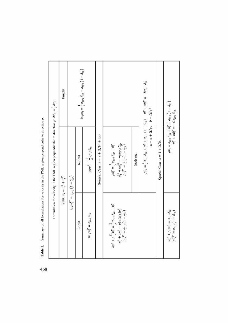
3 . 3 . T h e S u m m a r y o f t h e F o r m u l a t i o n s

All treated formulations are summarized in Table 1 which clearly maps different formulations and their relations. For conciseness the table lists only equations for the particle velocity. It is clear that the general form of the stretching factor s given by Eq.(19) naturally implies the additional functions (memory variables) in both the split and unsplit formulations if a direct calculation of the convolutional terms is to be avoided. In the case of the L-split formulation and special choice of the stretching factor, given by Eq.(36), the resulting equations reduce to the well known equations with a simple damping term - Eqs.(37) and (38). The case of the R-split formulation eventually leads to the equations identical with those obtained straightforwardly in the unsplit formulation.

4. TIME DISCRETIZATION OF THE UNSPLIT FORMULATION

Consider the following approximations at the time level m:

1 12 2, ,, 1

2

p m p mp mi i i

, (60)

1 12 2, ,, 1 p m p mp m

i i it . (61)

Application of approximations (60) and (61) to Eq.(50) yields

1 12 2, ,2 2

,2 2

p m p m mji j jpi i

a t b t

a t a t

. (62)

468

F

orm

ulat

ion

for

velo

city

in th

e PM

L r

egio

n pe

rpen

dicu

lar

to d

irec

tion

p:

Uns

plit

i1 ,

,1

Gen

eral

Cas

e:

Ωi⁄

,,1

,

, Ω⁄ ,

Ω⁄

Spec

ial C

ase:

1Ω

i⁄ ,,1

Ω

Ω,

Split

:

i,1

R-S

plit

i1 ,

1 , ,

,1

lead

s to

:

L-S

plit

i,

Ω1 ,

Ω⁄

,1

Ω,

,1

Tab

le 1

. Su

mm

ary

of a

ll fo

rmul

atio

ns f

or v

eloc

ity in

the

PML

reg

ion

perp

endi

cula

r to

dir

ecti

on p

.

469

If we relate Eq.(58) to the time level m, we need ,p mi . Using Eqs.(60) and (62) we obtain

12,, 2

,2 2

p mp m mji j jpi i

b t

a t a t

. (63)

Using Eq.(63) we can rewrite Eq.(58):

12,1 2

, , 12 2

p mm m mi ji j jp ji j jpi

b t

a t a t

v . (64)

Then the final form of the equation of motion with the memory variables and corresponding additional equations is obtained after substituting a and b from Eq.(41) in

Eqs.(62) and (64), and approximating miv by the central-difference formula:

1 12 2

12,

11 ,

2

2, 1 ,

2

m m mji j jpi i

p m mji j jpi

t t

t

t

v v (65)

1 12 2, ,2 1 2

,2 2

p m p m mji j jpi i

t t

t t

. (66)

The time discretization of the constitutive relation (59) and additional equations for the memory variables is analogous. The final system is

12

12

1

,

1,

2

2, 1 ,

2

mm mij ij ijkl l lpk

mp mijkl l lpij k

tt c

t

ct

v

v

(67)

12

, 1 ,2

2

1 2, .

2

p m p mij ij

mijkl l lpk

t

t

tc

t

v (68)

The discretization given by Eqs.(65)(68) is an alternative to the discretization presented by Komatitsch and Martin (2007). Their discretization can be written in the form similar to that in Eqs.(65)(68):

.

470

1 12 2

12,

exp 111 ,

2 2

exp 1, 1 ,

2

m m mji j jpi i

p m mji j jpi

tt

t

v v

(69)

1 12 2, ,

exp

1exp 1 , ,

p m p mi i

mji j jp

t

t

(70)

12

12

1

,

exp 111 ,

2 2

exp 1, 1 ,

2

mm mij ij ijkl l lpk

mp mijkl l lpij k

tt c

tc

v

v

(71)

12

, 1 ,exp

1exp 1 , .

p m p mij ij

mijkl l lpk

t

t c

v (72)

The difference between the two discretizations is in coefficients. It is due to different time integrations of Eqs.(50) and (51). The integration chosen by Komatitsch and Martin (2007) would be the exact integration in case of homogeneous Eqs.(50) and (51), that is if

0b . Both discretizations are 2nd-order accurate in time if 0b which is the case. Numerical tests are necessary to compare the two approaches.

5. NUMERICAL COMPARISON OF THE TWO DISCRETIZATIONS

We present numerical results for a wavefield generated by a point single force in a homogeneous isotropic elastic medium. The configuration is close to that considered by Komatitsch and Martin (2007). The 3D model of the relatively thin slice has shape of the rectangular parallelepiped with dimensions 1000 6400 6420 m3. P-wave speed, S-wave speed and density are, respectively, 3300 m/s, 1905.3 m/s and 2800 kg/m3. The point single-force source is located at x = 790 m, y = 4270 m, and z = 3210 m assuming that one corner of the rectangular parallelepiped is located at the origin of the Cartesian coordinate system and its short edge is parallel with the x-axis. The force is oriented at 135 in the (x,y) plane. The source-time function used in the numerical simulations is Gabor signal - a harmonic carrier with a Gaussian envelope,

2( ) exp cosp s s p ss t t t t t . Here, 2p pf , 0,2 st t ,

471

fp = 15 Hz is predominant frequency, s = 4 controls the width of the signal, = /2 is a

phase shift, and 0.45s s pt f .

The computational domain was covered with a uniform staggered grid. With the grid spacing of 10 m in the three Cartesian directions, the numbers of grid spacings in the three directions were 100, 640, and 640. The simulations for the interior grid were performed using the 4th-order in space, 2nd-order in time velocity-stress staggered-grid finite-difference scheme. A 100 m (10 grid spacings) thick PML was applied on the six sides of the parallelepiped. The same damping profile was applied in all coordinate directions:

20 L , , ,x y z , 0 = 341.9, L = 100 m. The other parameters are = 1,

= fp. For explanation of this choice see Komatitsch and Martin (2007). At the external boundaries of the PML (and thus the grid) the particle velocity is set equal to zero (rigid boundary). The finite-difference approximation applied in the PML is 2nd-order in space and time.

The time step was 1.4 ms. The simulated time window is 140 s, the number of performed time steps is 100 000.

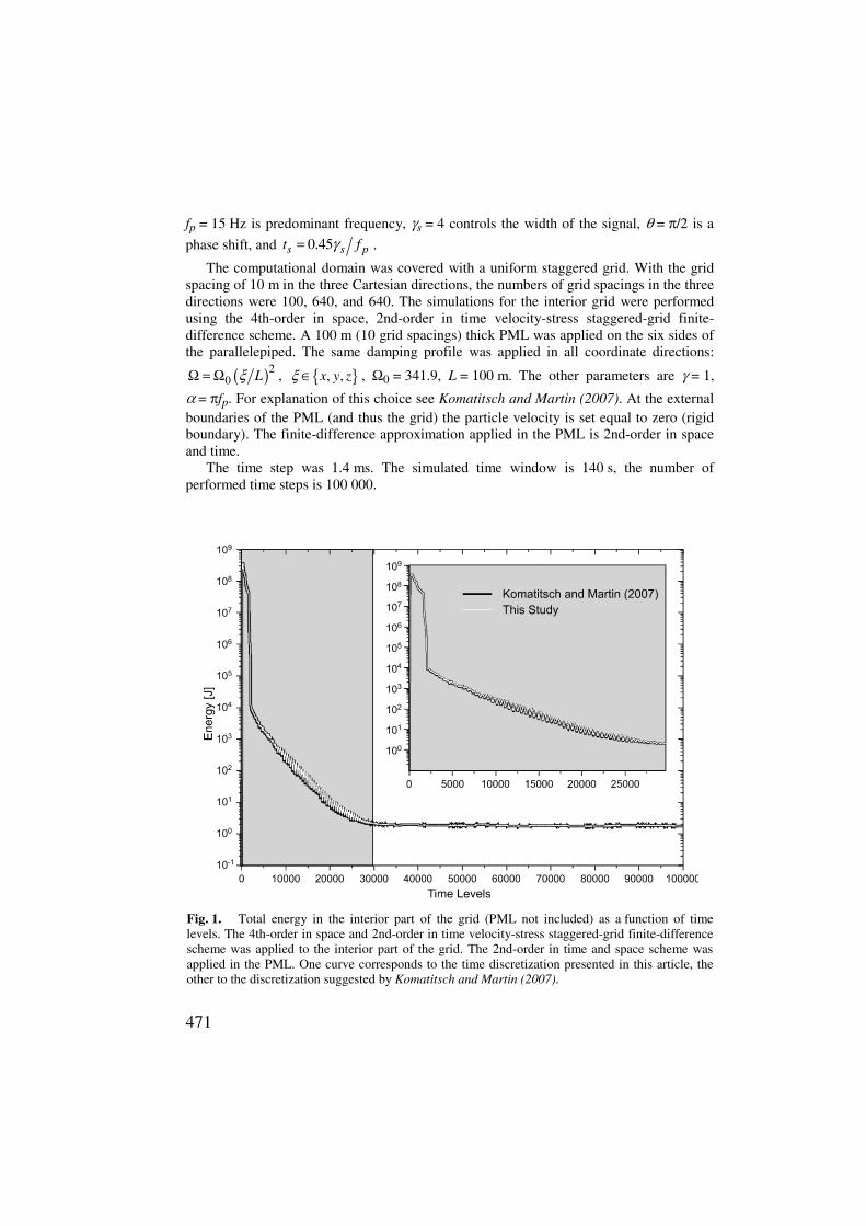
Fig. 1. Total energy in the interior part of the grid (PML not included) as a function of time levels. The 4th-order in space and 2nd-order in time velocity-stress staggered-grid finite-difference scheme was applied to the interior part of the grid. The 2nd-order in time and space scheme was applied in the PML. One curve corresponds to the time discretization presented in this article, the other to the discretization suggested by Komatitsch and Martin (2007).

472

Following Komatitsch and Martin (2007) we evaluate the total energy in the interior part of the grid (the PML excluded) as a function of time. The total energy, defined as

21 1

2 2 ij ijE v , (73)

should decay with time after the source stops radiating energy. Fig. 1 shows the total energy in the grid as a function of time level obtained by two numerical simulations. One simulation was performed with the use of our discretization, Eqs.(65)(68), the other with the use of the discretization presented by Komatitsch and Martin (2007), Eqs.(69)(72). The two curves practically coincide for all 100 000 time levels. We can see this agreement as a confirmation of accuracy of both discretizations. We note that the energy-decay curve differs slightly from that presented by Komatitsch and Martin (2007): The oscillations are due to the 4th-order scheme applied in the interior grid and not in the PML. We saw this clearly on the snapshots (not shown here). The resulting residual high-frequency numerical noise is responsible for the fact that the amount of energy stabilizes in the grid - the grid is not capable to “process” the high-frequency noise. However, the noise level is about 8 orders of magnitude weaker than the useful signal. Therefore it does not pose a practical problem.

6. CONCLUSIONS

The PML may be split or unsplit, classical or convolutional, with the general or special form of the stretching factor. We showed relations between different formulations of the PML with respect to their three key aspects.

We derived two variants of the split formulations for the general form of the stretching factor. The L-split variant has the stretching factor on the left-hand side of the equation of motion and constitutive law, the R-split variant on the right-hand side. Both variants naturally lead to convolutional formulations in case of the general form of the stretching factor. The L-split variant reduces to the well-known classical split formulation in case of the special form of the stretching factor. The R-split formulation remains convolutional even for the special form of the stretching factor.

The R-split formulation eventually leads to the equations identical with those obtained straightforwardly in the unsplit formulation.

We presented a time discretization of the unsplit formulation which is a slightly algorithmically simpler alternative to the time discretization presented by Komatitsch and Martin (2007). The latter is shown in the form consistent with our discretization. We implemented both discretizations in the 3D velocity-stress staggered-grid finite-difference scheme. The interior grid was solved with the 4th-order whereas the PML with the 2nd-order scheme in space, both being the 2nd-order in time. Numerical tests showed a very good level of agreement of the two discretizations.

Acknowledgements: This work was supported in part by the Slovak Research and Development

Agency under the contract No. APVV-0435-07 (project OPTIMODE), VEGA Project 1/4032/07, and ITSAK-GR MTKD-CT-2005-029627 Project.

473

References

Basu U., 2009. Explicit finite element perfectly matched layer for transient three-dimensional elastic waves. Int. J. Numer. Meth. Eng., 77, 151176.

Basu U. and Chopra A.K., 2004. Perfectly matched layers for transient elastodynamics of unbounded domains. Int. J. Numer. Meth. Eng., 59, 10391074.

Bérenger J.P., 1994. A perfectly matched layer for the absorption of electromagnetic waves. J. Comput. Phys., 114, 185200.

Bérenger J.P., 1996. Three-dimensional perfectly matched layer for the absorption of electromagnetic waves. J. Comput. Phys., 127, 363–379.

Chen Y.H., Coates R.T. and Robertsson J.O.A., 2000. Extension of PML ABC to Elastic Wave Problems in General Anisotropic and Viscoelastic Media. Schlumberger OFSR Research Note, Schlumberger, Cambridge, U.K.

Chew W.C. and Liu Q., 1996. Perfectly Matched Layers for elastodynamics: a new absorbing boundary condition. J. Comput. Acoust., 4, 341359.

Chew W.C. and Weedon W.H., 1994. A 3-D perfectly matched medium from modified Maxwell’s equations with stretched coordinates. Microw. Opt. Technol. Lett., 7, 599604.

Collino F. and Tsogka C., 2001. Applications of the PML absorbing layer model to the linear elastodynamic problem in anisotropic heterogeneous media. Geophysics, 66, 294305.

Drossaert F.H. and Giannopoulos A., 2007a. Complex frequency shifted convolution PML for FDTD modelling of elastic waves. Wave Motion, 44, 593604.

Drossaert F.H. and Giannopoulos A., 2007b. A nonsplit complex frequency-shifted PML based on recursive integration for FDTD modeling of elastic waves. Geophysics, 72, T9T17.

Festa G., Delavaud E. and Vilotte J.-P., 2005. Interaction between surface waves and absorbing boundaries for wave propagation in geological basins: 2D numerical simulations. Geophys. Res. Lett., 32, L20306.

Festa G. and Nielsen S., 2003. PML Absorbing Boundaries. Bull. Seismol. Soc. Amer., 93, 891903.

Festa G. and Vilotte J.P., 2005. The Newmark scheme as velocity-stress time-staggering: An efficient PML implementation for spectral-element simulations of elastodynamics. Geophys. J. Int., 161, 789812.

Komatitsch D. and Martin R., 2007. An unsplit convolutional Perfectly Matched Layer improved at grazing incidence for the seismic wave equation. Geophysics, 72, SM155SM167.

Komatitsch D. and Tromp J., 2003. A perfectly matched layer absorbing boundary condition for the second-order seismic wave equation. Geophys. J. Int., 154, 146153.

Marcinkovich C. and Olsen K., 2003. On the implementation of perfectly matched layers in a three-dimensional fourth-order velocity-stress finite difference scheme. J. Geophys. Res., 108, 22762292.

Ma S. and Liu P., 2006. Modeling of the perfectly matched layer absorbing boundaries and intrinsic attenuation in explicit finite-element methods. Bull. Seismol. Soc. Amer., 96, 17791794.

Martin R. and Komatitsch D., 2006. An optimized convolution-perfectly matched layer (C-PML) absorbing technique for 3D seismic wave simulation based on a finite-difference method. Geophys. Res. Abstracts, 8, 03988.

474

Martin R., Komatitsch D. and Barucq H., 2005. An optimized Convolution-Perfectly Matched Layer (C-PML) absorbing technique for 3D seismic wave simulation based on a finite-difference method. Eos Trans. AGU, 86(52), Fall Meet. Suppl., Abstract NG43B-0574.

Martin R., Komatitsch D. and Ezziani A., 2008a. An unsplit convolutional perfecly matched layer improved at grazing incidence for seismic wave equation in poroelastic media. Geophysics, 73, T51T56.

Martin R., Komatitsch D. and Gedney S.D., 2008b. A variational formulation of a stabilized unsplit convolutional perfectly matched layer for the isotropic or anisotropic seismic wave equation. Comput. Model. Eng. Sci., 37, 274304.

Moczo P., Robertsson J.O.A. and Eisner L., 2007. The finite-difference time-domain method for modeling of seismic wave propagation. In: Wu R.-S. and Maupin V. (Eds.), Advances in Wave Propagation in Heterogeneous Earth. Advances in Geophysics, 48, Elsevier, Amsterdam, The Netherlands, 421516.

Wang T. and Tang X., 2003. Finite-difference modeling of elastic wave propagation: A nonsplitting perfectly matched layer approach. Geophysics, 68, 17491755.