a brief introduction of dqmc study in itinerant quantum criticalpoint

Zi Hong LiuSeptember 2018

Institute of Physics Chinese Academy of Sciences

Collaborators

1

Outlines

IntroductionModelPhysical significance

Transverse field Ising model

Mean field analysis

The free fermion Hamiltonian

Two layers constructionDeterminant Quantum Monte Carlo

Path integral of the partition function

Operator and Measurment

Sampling in DQMC

Numerical StabilizationExample

2

introduction

Introduction

∙ Strong correlated itinerant electron system;∙ Nonperturbative nature;∙ The Determinant quantum monte carlo(DQMC) method.

4

model

general strong correlated itinerant electron system

H = Hfermion +Hspin +Hf−s +Hf−f , (1)

Hfermion = −tij∑

ij,α c†iαcjα + h.c.− µ∑

i ni

Hspin = −J∑

ij szi s

zj − hx

∑i

sxi

Hf−s = −ξ∑

ijk,αβ c†iαszk cjβ

Hf−f = −VI

∑ijkl,αβγδ c

†iαc

†jβ ckγ clδ

, (2)

6

Spin-Fermion Model

Hfermion = −t

∑⟨ij⟩σλ c†iλσ cjλσ + h.c.− µ

∑iσλ niλσ

Hspin = −J∑⟨ij⟩

szi szj − hx

∑i s

xi

Hf−s = −ξ∑

i szi (c

†i τzσz ci) = −ξ

∑i s

zi (σ

zi1 − σz

i2)

. (3)

7

physical significance

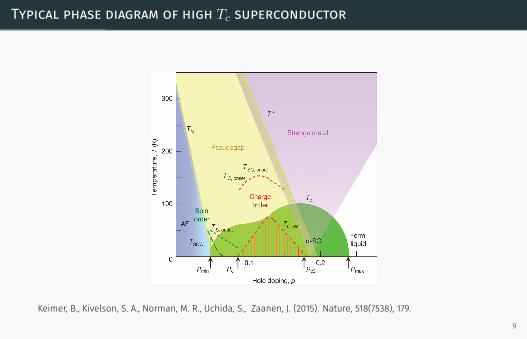
Typical phase diagram of high Tc superconductor

Keimer, B., Kivelson, S. A., Norman, M. R., Uchida, S., Zaanen, J. (2015). Nature, 518(7538), 179.

9

0 0.1 0.2 0.30

0.1

0.2

0.3

0.4

0.5

ε

1.5

1.0

2.0

YbRh2(Si

0.95Ge

0.05)

2

B ⊥c

B(T)

T(K

)

2

0 10

0.1

0.2

0.3

YbRh2Si

2

B ��c

2

B(T)

T(K

)

Nature 424, 524-527 (2003)

10

Transverse field Ising model

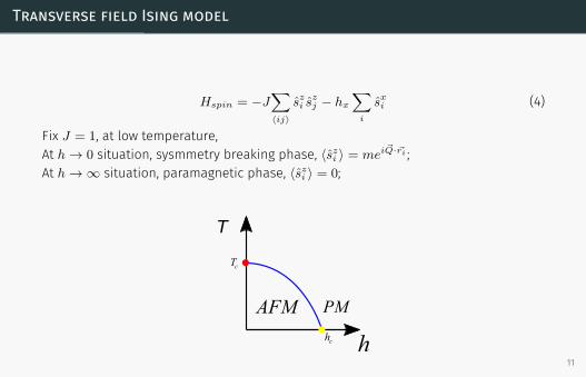
Hspin = −J∑⟨ij⟩

szi szj − hx

∑i

sxi (4)

Fix J = 1, at low temperature,At h → 0 situation, sysmmetry breaking phase, ⟨szi ⟩ = meiQ·ri ;At h → ∞ situation, paramagnetic phase, ⟨szi ⟩ = 0;

T

h

AFM PM

Tc

hc

11

Mean field analysis

The Ising spin and fermion coupling term make fermion behavior differently in Isingparamagentic(PM) and Ising symmetry breaking phases.

∙ At h → ∞, we can replace szi by ⟨szi ⟩ = 0.∙ At h → 0, we can replace szi by ⟨szi ⟩ = meiQ·ri .

Hf−s = −ξ∑i

szi (c†i τzσz ci) → −ξ

∑i

⟨szi ⟩ (c†i τzσz ci) (5)

12

ci =1√N

∑k∈BZ

ckeik·ri , ck =

1√N

∑i

cie−ik·ri , (6)

1

N

∑i

e−i(k−k′)·ri = δkk′ (7)

13

∑⟨ij⟩

c†i1↑cj1↑ =∑i

∑l

c†i1↑ci+l,1↑ =1

N

∑i

∑l

∑kk′

c†k1↑ck′1↑e−i(k−k′)·rieik·l

=∑k

∑l

c†k1↑ck1↑eik·l =

∑k

(∑l

eik·l)nk1↑

, (8)

µ∑i

ni1↑ = µ 1N

∑i

∑kk′

c†k1↑ck′1↑e−i(k−k′)·ri

= µ∑k

nk1↑, (9)

ξ∑i

meiQ·ri ni1↑ = ξm1

N

∑i

∑kk′

c†k1↑ck′1↑e−i(k−k′−Q)·ri

= ξm∑k

c†k+Q,1↑ck1↑, (10)

14

Define ϵ(k) =

(−t∑l

eik·l + h.c.− µ

), and dk = ck+Q then

Hfermion−eff =∑

k∈BZ

(−t∑l

eik·l + h.c.− µ

)nk1↑ − ξm

∑k∈BZ

c†k+Q,1↑ck1↑

=∑

k∈BZ

ϵ(k)nk1↑ − ξm∑

k∈NBZ

d†k,1↑ck1↑ − ξm∑

k∈NBZ

c†k,1↑dk1↑

=∑

k∈NBZ

ϵ(k)c†k1↑ck1↑ +∑

k∈NBZ

ϵ(k +Q)d†k1↑dk1↑−

ξm∑

k∈NBZ

d†k,1↑ck1↑ − ξm∑

k∈NBZ

c†k,1↑dk1↑

,

(11)and

Hfermion−eff =[c†k1↑ d†k1↑

] [ ϵ(k) −ξm

−ξm ϵ(k +Q)

][ck1↑

dk1↑

]. (12)

15

Hfermion−eff =[c†k1↑ d†k1↑

] [ ϵ(k) −ξm

−ξm ϵ(k +Q)

][ck1↑

dk1↑

]. (13)

∙ The perfect nesting condition ϵ(k +Q) = −ϵ(k).∙ The eigenvalue of the matrix E±

k = ±√

ϵ2(k) + ξ2m2.∙ Fermi surface, ϵ(k) = 0, so E±

k = ±ξm the energy gap ∆ = 2ξm.

16

The band folding and gap opening due to magnetic order with wave vector in onedimensional system, ϵ(k) = − cos(k) and Q = π, ϵ(k +Q) = cos(k).

- 0

Ef

- 0

Ef

In two dimension, in hall filling square lattice, ϵ(k) = −cos(kx)− cos(ky), Q = (π, π),ϵ(k +Q) = −ϵ(k) satisfy in the whole Fermi-surface.

17

The free fermion Hamiltonian

Hfermion = −tij∑ij,α

c†iαcjα + h.c.− µ∑i

ni =∑k

ϵ(k)c†k ck. (14)

18

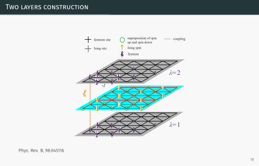
Two layers construction

fermion site

Ising site

coupling

Ising spin

fermion

superposition of spin up and spin down

λ=1

λ=2

-t

Phys. Rev. B, 98:045116

19

determinant quantum monte carlo

Determinant Quantum Monte Carlo

∙ R. Blankenbecler, D. J. Scalapino, and R. L. Sugar. i. Phys. Rev. D, 24:2278–2286, Oct1981.

∙ Hirsch, Phys. Rev. B 28, 4059(R) (1983)∙ Hirsch, Phys. Rev. B 31, 4403 (1985)

∙ F.F. Assaad and H.G. Evertz. Springer Berlin Heidelberg, 2008.∙ Xiao Yan Xu. PhD thesis, Institute of Physics (IOP), Chinese Academy of Sciences,2017.

21

Free fermion partition function

Free fermion HamiltonianH0 =

∑ij

c†iTij cj = c†T c (15)

Z = Tr{e−βH} = Tr{e−βc†T c} = Tr{e−β∑

ij c†iTij cj}

= Tr{e−β(Uc)†U†TUc} = Tr{e−β∑

k ϵ(k)nk}=

∏k

∑nk=0,1

e−βϵ(k)nk = det(1+ e−βT ). (16)

22

Hubbard-Stratonovich(HS) transformation

H = H0 +HI . (17)The general four fermion interaction is

Hf−f = −VI

∑ijkl,αβγδ

c†iαc†jβ ckγ clδ, (18)

The HS transformation

∙ Continuous version

eK2

2 =1√2π

∞∫−∞

dϕe−ϕ2

2−ϕK . (19)

∙ Four components

e∆τWK2

=1

4

∑l=−2,−1,1,2

γ(l) exp(√∆τWη(l)K) +O(∆τ4). (20)

F.F. Assaad, arXiv:cond-mat/9806307

23

Trotter decomposition

Z = Tr{e−βH} = Tr{(e−∆τHI e−∆τH0)M}+O(∆τ2)

=∑C

WSC Tr{

1∏τ=M

ec†V (C)ce−∆τc†T c}+O(∆τ2)

. (21)

Define

U(τ2, τ1) =

n2∏n=n1+1

ec†V (C)ce−∆τc†T c, (22)

B(τ2, τ1) =

n2∏n=n1+1

eV (C)e−∆τT . (23)

We can write down the partition function to a much concise form,

Z =∑C

WSC Tr{U(β, 0)} (24)

After tracing out fermion degrees of freedom, we obtain

Z =∑C

WSC det[1+B(β, 0)]. (25)

24

Path integral to transverse field Ising model

To the bare transverse field Ising model Hspin.

Hspin = −J∑ij

szi szj − hx

∑i

sxi (26)

Z = Tr{e−βHspin}

=

∏τ

∏⟨ij⟩

e∆τJ

∑⟨ij⟩s

zi,τs

zj,τ

∏i

∏⟨τ,τ ′⟩

Λeγ∑

⟨ij⟩szi,τs

zj,τ ′

+O(∆τ2).

(27)

25

Partition function of spin-fermion model

Hfermion = −t

∑⟨ij⟩σλ c†iλσ cjλσ + h.c.− µ

∑iσλ niλσ

Hspin = −J∑⟨ij⟩

szi szj − hx

∑i s

xi

Hf−s = −ξ∑

i szi (c

†i τzσz ci) = −ξ

∑i s

zi (σ

zi1 − σz

i2)

. (28)

Z =∑{Sz}

WT IC WF

C +O(∆τ2) . (29)

WT IC =

∑{Sz}

(∏τ

∏⟨ij⟩e

∆τJ∑

⟨ij⟩szi,τs

zj,τ

)(∏i

∏⟨τ,τ ′⟩Λe

γ∑

⟨ij⟩szi,τs

zj,τ ′)

(30)

WFC = det[1+B(β, 0)] (31)

26

Operator and Measurment

In statistical mechanics, the ensemble average of physical observable can be expressas ⟨

O⟩=

Tr{e−βHO}Tr{e−βH}

=∑C

PC

⟨O⟩C+O(∆τ2) (32)

PC =WS

C det[1+B(β, 0)]∑C WS

C det[1+B(β, 0)], (33)

⟨O⟩C=

Tr{U(β, τ)OU(τ, 0)}Tr{U(β, 0)}

. (34)

Equal time Green’s function

(Gij)C =⟨cic

†j

⟩C= (1+B(τ, 0)B(β, τ))−1

ij . (35)

27

The time dependent Green’s function

The time dependent Green’s function is

(Gij(τ1, τ2))C =⟨Tτ ci(τ1)c

†j(τ2)

⟩C, (36)

where Tτ is time-ordering operator. When τ1 > τ2, we can obtain

(Gij(τ1, τ2))C =⟨ci(τ1)c

†j(τ2)

⟩C

=Tr{U(β,τ1)ciU(τ1,τ2)c

†j U(τ2,0)}

Tr{U(β,0)}

=Tr{U(β,τ2)U

−1(τ1,τ2)ciU(τ1,τ2)c†j U(τ2,0)}

Tr{U(β,0)}

. (37)

(Gij(τ1, τ2))C = [B(τ1, τ2)GC(τ2, τ2)]ij . (38)

28

Sampling in DQMC

If we can make the configurations generated according to the distribution define byPC , the ensemble average of observable will be⟨

O⟩=

1

Nsample

sample∑i=1

⟨O⟩Ci

, (39)

1. Detail Balance Condition:

WCT (C → C′) = WC’T (C′ → C). (40)

2. Ergodic Condition: All states are aperiodic and positive recurrent

29

Sign problem

Map probability to PC , when PC = PC

⟨O⟩=

Tr{e−βHO}Tr{e−βH}

=∑C

PC

⟨O⟩C+O(∆τ2) (41)

Reweight scheme in measurement, Map probability to PC ,

⟨O⟩=

⟨sign e−S

R{e−S} ⟨O⟩⟩

P⟨sign⟩

P

, (42)

30

Hfermion = −t∑

⟨ij⟩σλ c†iλσ cjλσ + h.c.− µ∑

iσλ niλσ

Hf−s = −ξ∑

i szi (c

†i τzσz ci) = −ξ

∑i s

zi (σ

zi1 − σz

i2). (43)

The Hamiltonian is block diagonal as four orbitals, which is

(τz, σz) = [↑ 1, ↓ 1, ↑ 2, ↓ 2]. (44)

We can see H↑1 = H↓2, H↑2 = H↓1. Regroup four orbitals into two superpositionorbitals

(α1, α2) = [(↑ 1, ↓ 2), (↑ 2, ↓ 1)]. (45)

In the two regroup orbitals, Hα1 = Hα2 , so

det(1+B(β, 0)) =∏2

i=1 det(1+Bαi(β, 0)) = |det(1+Bα1(β, 0))|2 . (46)

So our designer model is free of sign problem.

31

Fast Update

Local update, Metropolis-Hastings algorithm.

A(C → C′) = min

[1,

WC′

WC

]. (47)

For the onsite coupling feature, V (C) is a diagonal matrix with

exp(V 1↑i (C)) = exp(V 1↑(si)) = exp(∆τξsi). (48)

In single auxillary field update scheme,

eV1↑i (C′) = exp(∆τξs′i) = (1 + (e∆τξs′ie−∆τξsi − 1))e∆τξsi = (1 +∆ii)e

V1↑i (C), (49)

where ∆ii = e∆τξs′ie−∆τξsi − 1.

32

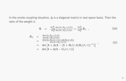
In the onsite coupling situation, ∆ is a diagonal matrix in real space basis. Then theratio of the weight is

R =WS

C′ det(1+BC′ (β,0))

WSC det(1+BC(β,0))

=WS

C′WS

CRf , (50)

Rf =det(1+BC′ (β,0))det(1+BC(β,0))

= det(1+BC(β,τ)(1+∆)BC(τ,0))det(1+BC(β,0))

= det[1+∆(1− (1+BC(τ, 0)BC(β, τ))

−1)]

= det [1+∆(1−GC(τ, τ))]

, (51)

33

If update is accepted, we also need update Green’s function

GC′(τ, τ) = [1+ (1+∆)BC(τ, 0)BC(β, τ)]−1 (52)

= [1+BC(τ, 0)BC(β, τ)]−1 × (53)[

(1+ (1+∆)BC(τ, 0)BC(β, τ))((1+BC(τ, 0)BC(β, τ))

−1)]−1

as GC(τ, τ) = [1+BC(τ, 0)BC(β, τ)]−1, we denote AC ≡ BC(τ, 0)BC(β, τ) ≡ G−1

C − 1,

GC′(τ, τ) = GC [(1+ (1+∆)AC)GC ]−1

= GC[(1+ (1+∆)

(G−1

C − 1))

GC]−1 (54)

= GC [1+∆(1−GC)]−1

34

Rf = 1 +∆ii(1−GCii) (55)

GC′(τ, τ) = GC(τ, τ) + αiGC(:, i) (GC(i, :)− ei) (56)

, αi = ∆ii/Rf .Computational complexity: O(N2) for each auxillary field update, O(βN3) for onesweep.

35

Global Update

∙ Critical slowing down;∙ Self learning Monte Carlo;

MachineLearning

(ii)Trial simulation by local update(i)

Ηeff

Learning

Ηeff

Detailedbalance

Η

(iii) (iv)

Proposetrial Conf.

Simulating

Phys. Rev. B, 95:041101

36

Numerical Stabilization

∙ The condition number of fermion determinant;∙ The singular value decompositions (SVD);∙ O(N3) computational complexity;

B(nτw, 0) = Un

X

XX

X

︸ ︷︷ ︸

Dn

Vn, (57)

τw = Nst∆τ

37

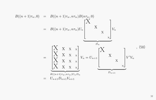
B((n+ 1)τw, 0) = B((n+ 1)τw, nτw)B(nτw, 0)

= B((n+ 1)τw, nτw)Un

X

XX

X

︸ ︷︷ ︸

Dn

Vn

=

X X X X

X X X X

X X X X

X X X X

︸ ︷︷ ︸B((n+1)τw,nτw)UnDn

Vn = Un+1

X

XX

X

︸ ︷︷ ︸

Dn+1

V ′Vn

= Un+1Dn+1Vn+1

, (58)

38

G(τ, τ)

= [1 +B(τ, 0)B(β, τ)]−1

= [1 + URDRVRVLDLUL]−1

= U−1L

[(ULUR)

−1 +DR (VRVL)DL

]−1U−1

R

= U−1L

[(ULUR)

−1 +DmaxR Dmin

R (VRVL)DminL Dmax

L

]−1

U−1R

= U−1L (Dmax

L )−1[(Dmax

R )−1 (ULUR)−1 (Dmax

L )−1 +DminR VRVLD

minL

]−1

(DmaxR )−1 U−1

R

= UL (DmaxL )−1

[(Dmax

R )−1(U†

LUR

)−1

(DmaxL )−1 +Dmin

R VRV†LD

minL

]−1

(DmaxR )−1 U−1

R

where DR = DmaxR Dmin

R , DL = DminL Dmax

L

39

example

Example

Hfermion = −t1∑

⟨ij⟩σλ

c†iλσ cjλσ − t2∑

⟨⟨ij⟩⟩σλ

c†iλσ cjλσ−

t3∑

⟨⟨⟨ij⟩⟩⟩σλ

c†iλσ cjλσ + h.c.− µ∑iσλ

niλσ

Hspin = −J∑⟨ij⟩

szi szj − hx

∑i

sxi

Hf−s = −ξ∑i

szi (c†i τzσz ci) = −ξ

∑i

szi (σzi1 − σz

i2)

, (59)

arXiv:1808.08878

41

0

0.2

0.4

0.6

0.8

1

2.6 2.8 3 3.2 3.4 3.6 3.8

T

h

Pure Boson hc=3.044(3)DQMC hc=3.32(2)EQMC hc=3.355(5)

b cafermion site

Ising site

couplingIsing spin

fermion

λ=1

λ=2

-t22

-t1

-t3

hJ

‘

(-π,π)

(-π,−π)

(π,π)

(π,−π)

K1

K1

K2 K3

K4

‘

K3

‘

K2

‘

K4

Q1 Q

3

Q2

Q4

k

k

x

y

Q1

QQ

Q3

4 2

K1

K

’

K

4K

2

K

3

K

1 K

2

K4

’

’’

3

arXiv:1808.08878

42

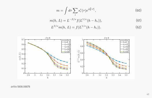
m =

∫dτ∑i

szi (τ)eiQ·ri , (60)

m(h, L) = L−β/νf(L1/ν(h− hc)), (61)

Lβ/νm(h, L) = f(L1/ν(h− hc)). (62)

2.9 3 3.1 3.2 3.3 3.4 3.5

h

0

0.1

0.2

0.3

0.4

0.5

0.6

0.7

m(h,L)

β = 4

L=8

L=12

L=16

L=20

L=24

2.9 3 3.1 3.2 3.3 3.4 3.5

h

0

0.2

0.4

0.6

0.8

1

Lβ/νm(h,L

)

β = 4

L=8

L=12

L=16

L=20

L=24

arXiv:1808.08878

43

G(k, τ > 0) =

∫ ∞

−∞dω

e−ω(τ−β/2)

2 cosh(βω/2)A(k, ω). (63)

limβ→∞

G(k, τ =β

2) = βA(k, ω = 0). (64)

High

Lowhkjjkj

High (a) (b)

h<hc h=hcarXiv:1808.08878

44

Demo code for dqmc

http://ziyangmeng.iphy.ac.cn/teaching.html

45