Quantum Critical Behavior

of

Disordered Itinerant Ferromagnets

D. Belitz – University of Oregon, USA

T.R. Kirkpatrick – University of Maryland, USA

M.T. Mercaldo – Università di Salerno, Italy

S.L. Sessions – University of Oregon, USA

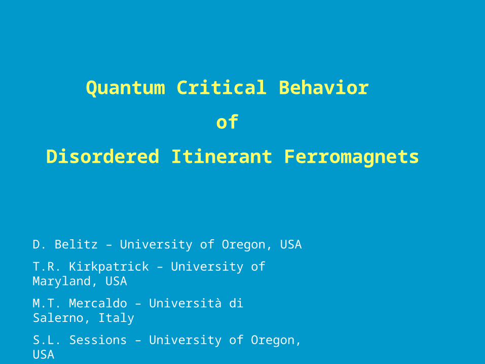
• Introduction: the relevance of quantum fluctuations

• phenomenology of QPT

• Quantum critical behavior of disordered itinerant FM

• Theoretical backgrounds:• Hertz Theory• Disordered Fermi Liquid

• The new approach • Microscopic theory• Derivation of the effective action• Behavior of observables

• Experiments

• Conclusion

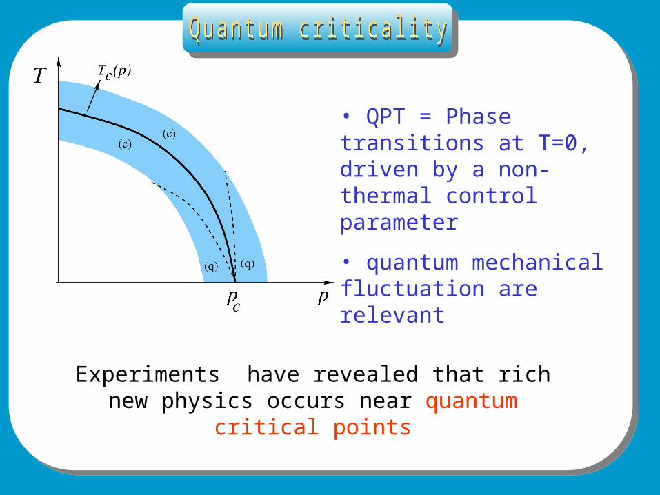
• QPT = Phase transitions at T=0, driven by a non-thermal control parameter

• quantum mechanical fluctuation are relevant

Experiments have revealed that rich new physics occurs near quantum critical points

Quantum criticality 2

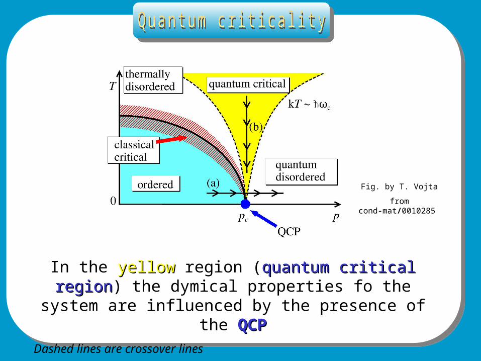
In the yellowyellow region (quantum critical regionquantum critical region) the dymical properties fo the system are influenced by the

presence of the QCPQCP

Dashed lines are crossover lines

Fig. by T. Vojta

from cond-mat/0010285

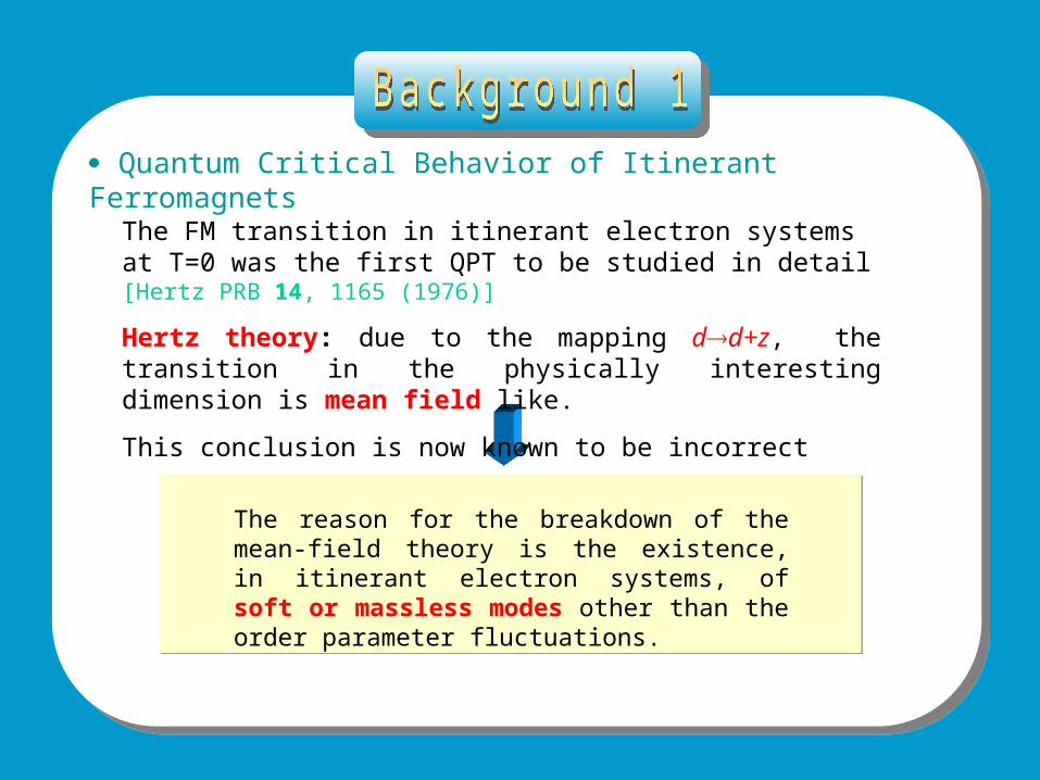
Quantum Critical Behavior of Itinerant Ferromagnets

The FM transition in itinerant electron systems at T=0 was the first QPT to be studied in detail [Hertz PRB 14, 1165 (1976)]

Hertz theory: due to the mapping dd+z, the transition in the physically interesting dimension is mean field like.

This conclusion is now known to be incorrect

The reason for the breakdown of the mean-field theory is the existence, in itinerant electron systems, of soft or massless modes other than the order parameter fluctuations.

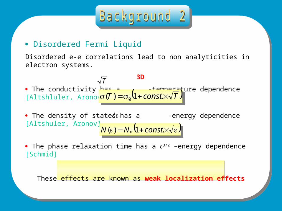
Disordered Fermi Liquid

Disordered e-e correlations lead to non analyticities in electron systems.

3D

The conductivity has a -temperature dependence [Altshluler, Aronov]T

TconstT .1)( 0 TconstT .1)( 0

The density of states has a -energy dependence [Altshuler, Aronov]

.1)( constNN F .1)( constNN F

The phase relaxation time has a 3/2 –energy dependence [Schmid]

These effects are known as weak localization effects

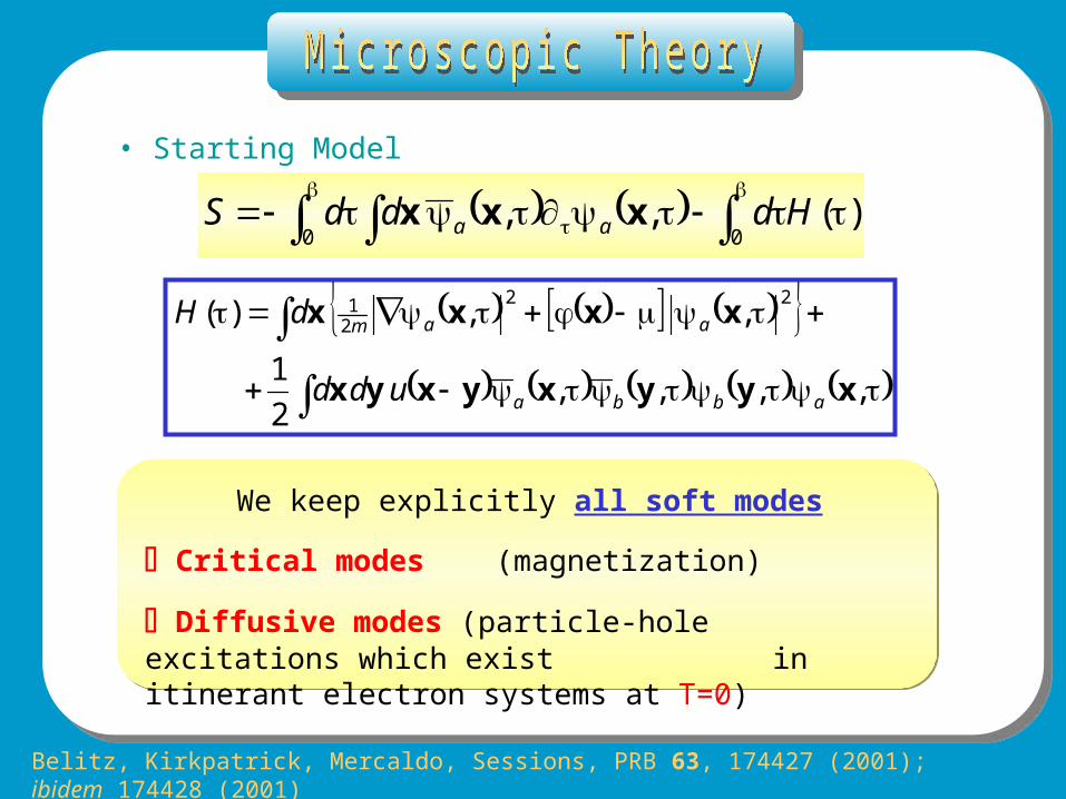
• Starting Model

)(,,00

HdddS aa xxx

,,,,

2

1

,,)(22

21

xyyxyxyx

xxxx

abba

aam

udd

dH

We keep explicitly all soft modes

Critical modes (magnetization)

Diffusive modes (particle-hole excitations which exist in itinerant electron systems at T=0)

Belitz, Kirkpatrick, Mercaldo, Sessions, PRB 63, 174427 (2001); ibidem 174428 (2001)

• Interaction term

Sint=Sint(s) + Sint

(t)

,,,

,,,

)(2

1

xxx

xxx

xx

bab

as

aac

t

n

n

ud

Using the Hubbard-Stratonovich transformation we decouple the Sint

(t) term and introduce explicitly the magnetization in the problem

Using the Hubbard-Stratonovich transformation we decouple the Sint

(t) term and introduce explicitly the magnetization in the problem

,,2 0

)(int xxx cc

ss nnddS

,,2 0

)(int xxx ss

tt nnddS

,,2

,,

0

0

)(int

xxx

xxx

st

t

nMdd

MMddS

,,2

,,

0

0

)(int

xxx

xxx

st

t

nMdd

MMddS

• Rewrite the fermionic degrees of freedom in terms of bosonic matrix fields

This formulation is particularly well suited for a separation of soft and massive modes

• Write explicitly soft and massive modes

• Integrate out massive modes

Aeff = AGLW[M] + ANLM[q] + Ac[M,q]Aeff = AGLW[M] + ANLM[q] + Ac[M,q]

details

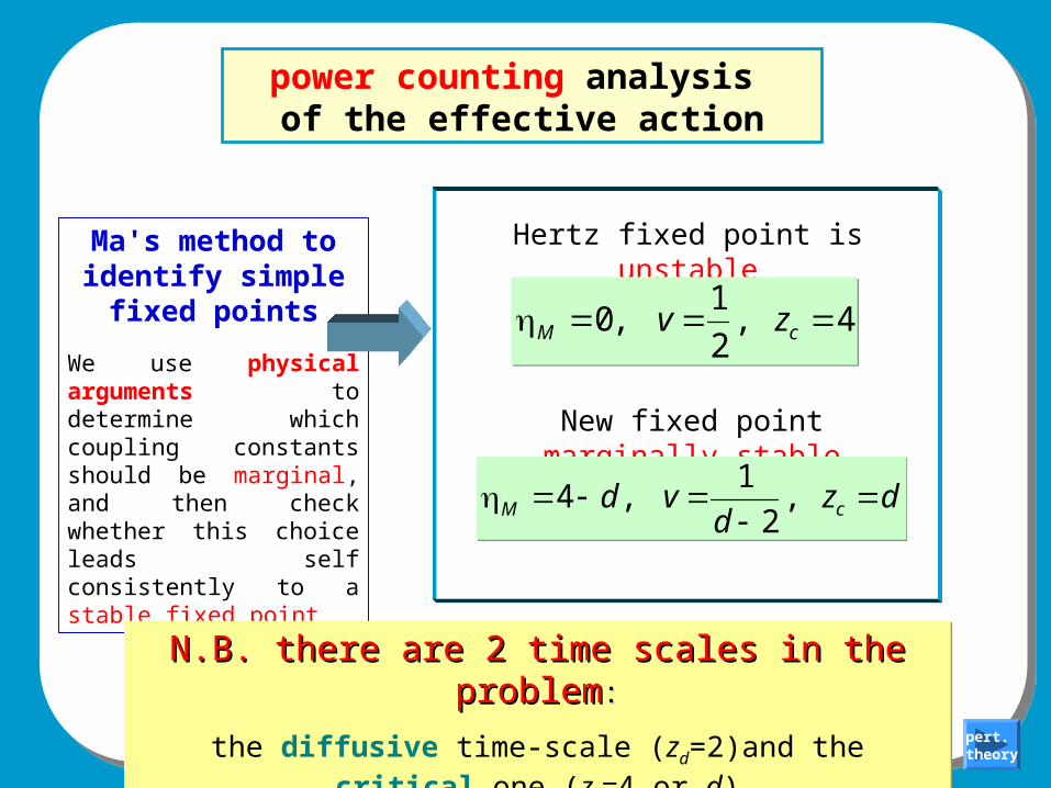
power counting analysis of the effective action

Ma's method to identify simple fixed

points

We use physical arguments to determine which coupling constants should be marginal, and then check whether this choice leads self consistently to a stable fixed point

Hertz fixed point is unstable

4,2

1,0 cM zv 4,

2

1,0 cM zv

New fixed point marginally stable

dzd

vd cM

,2

1,4 dz

dvd cM

,

2

1,4

N.B. there are 2 time scales in the problemN.B. there are 2 time scales in the problem::

the diffusive time-scale (zd=2)and the critical one (zc=4 or d)

N.B. there are 2 time scales in the problemN.B. there are 2 time scales in the problem::

the diffusive time-scale (zd=2)and the critical one (zc=4 or d)pert.

theory

b

bgz

b

bgdz

d

c

ln

)(lnln2

ln

)(lnln

b

bgd

b

bgd

ln

)(lnln2

1ln

)(lnln4

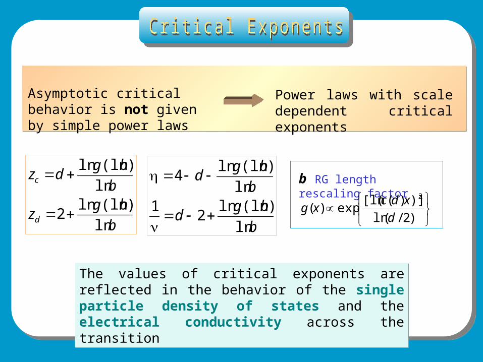
b RG length rescaling factor

)2/(ln

)])(([lnexp)(

2

d

xdcxg

The values of critical exponents are reflected in the behavior of the single particle density of states and the electrical conductivity across the transition

The values of critical exponents are reflected in the behavior of the single particle density of states and the electrical conductivity across the transition

Power laws with scale dependent critical exponents

Asymptotic critical behavior is not given by simple power laws

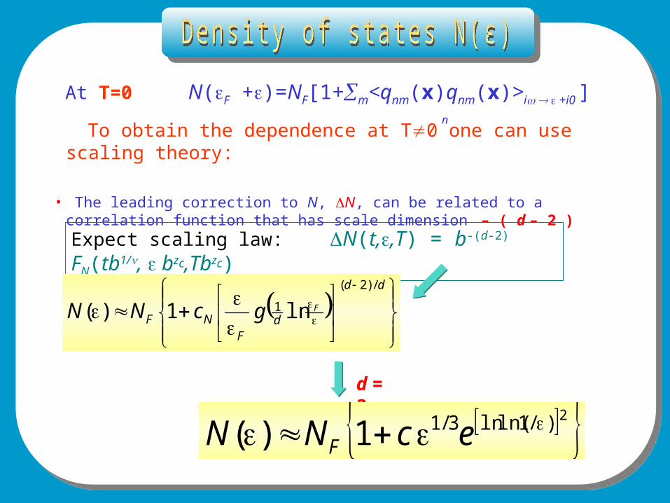
Density of states At T=0 N(F +)=NF[1+m<qnm(x)qnm(x)>i +i0 ]

To obtain the dependence at T0 one can use scaling theory:

• The leading correction to N, N, can be related to a correlation function that has scale dimension – ( d – 2 )

Expect scaling law: N(t,,T) = b-(d-2) FN(tb1/, bzc,Tbzc)

dd

dF

NFFgcNN

/)2(

1 ln1)(

d = 3

2)/1ln(ln3/11)( ecNN F

n

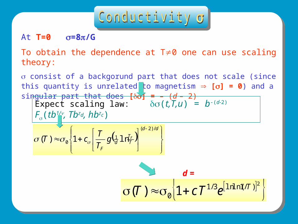
conductivityAt T=0 =8/G

To obtain the dependence at T0 one can use scaling theory:

consist of a backgorund part that does not scale (since this quantity is unrelated to magnetism [] = 0) and a singular part that does [] = – (d – 2)

• unrelated to magnetism [] = 0

• perturbation theory depends on critical dynamics (z) and on leading irrelevant operator u

• u is related to diffusive electrons [u] = d – 2

Expect scaling law: (t,T,u) = b-(d-2) F(tb1/, Tbzd, hbzc)

dd

TT

dF

FgT

TcT

/)2(

10 ln1)(

d = 3

2)/1ln(ln3/10 1)( TeTcT

Exp 1

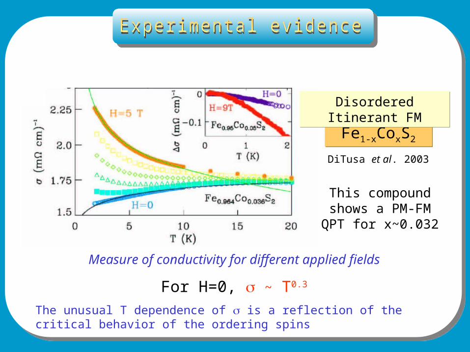
Fe1-xCoxS2Fe1-xCoxS2

DiTusa et al. 2003cond-mat/0306

Measure of conductivity for different applied fields

For H=0, ~ T0.3

The unusual T dependence of is a reflection of the critical behavior of the ordering spins

This compound shows a PM-FM QPT

for x~0.032

Disordered Itinerant FMDisordered Itinerant FM

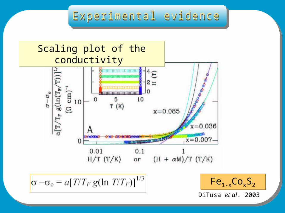
Fe1-xCoxS2Fe1-xCoxS2

DiTusa et al. 2003

Scaling plot of the conductivity Scaling plot of the conductivity Exp 1

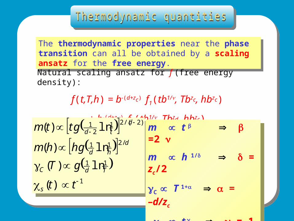
Thermodynamics quantities

The thermodynamic properties near the phase transition can all be obtained by a scaling ansatz for the free energy.

The thermodynamic properties near the phase transition can all be obtained by a scaling ansatz for the free energy.

Natural scaling ansatz for f (free energy density):

f(t,T,h) = b-(d+zc) f1(tb1/, Tbzc, hbzc)

+ b-(d+zd) f2(tb1/, Tbzd, hbzc)

22

22

/

/

/

hf

Tf

hfm

s

C

22

22

/

/

/

hf

Tf

hfm

s

C

1

11

/211

)2/(212

1

)(

ln)(

ln)(

ln)(

tt

gT

ghhm

gttm

s

TdC

d

hd

d

td 1

11

/211

)2/(212

1

)(

ln)(

ln)(

ln)(

tt

gT

ghhm

gttm

s

TdC

d

hd

d

td m t =2

m h 1/ = zc/2

C T 1+ = –d/zc

s t = 1

m t =2

m h 1/ = zc/2

C T 1+ = –d/zc

s t = 1

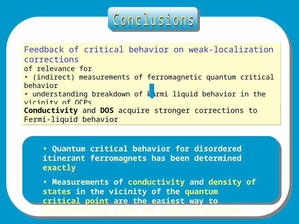
• Quantum critical behavior for disordered itinerant ferromagnets has been determined exactly

• Measurements of conductivity and density of states in the vicinity of the quantum critical point are the easiest way to experimentally probe the critical behavior

Feedback of critical behavior on weak-localization corrections of relevance for • (indirect) measurements of ferromagnetic quantum critical behavior • understanding breakdown of Fermi liquid behavior in the vicinity of QCPs

Feedback of critical behavior on weak-localization corrections of relevance for • (indirect) measurements of ferromagnetic quantum critical behavior • understanding breakdown of Fermi liquid behavior in the vicinity of QCPs

Conductivity and DOS acquire stronger corrections to Fermi-liquid behaviorConductivity and DOS acquire stronger corrections to Fermi-liquid behavior