Embed Size (px)
Citation preview
Iterative Deepening and Branch & Bound
CPSC 322 – Search 6
Textbook § 3.7.3 and 3.7.4
January 24, 2011
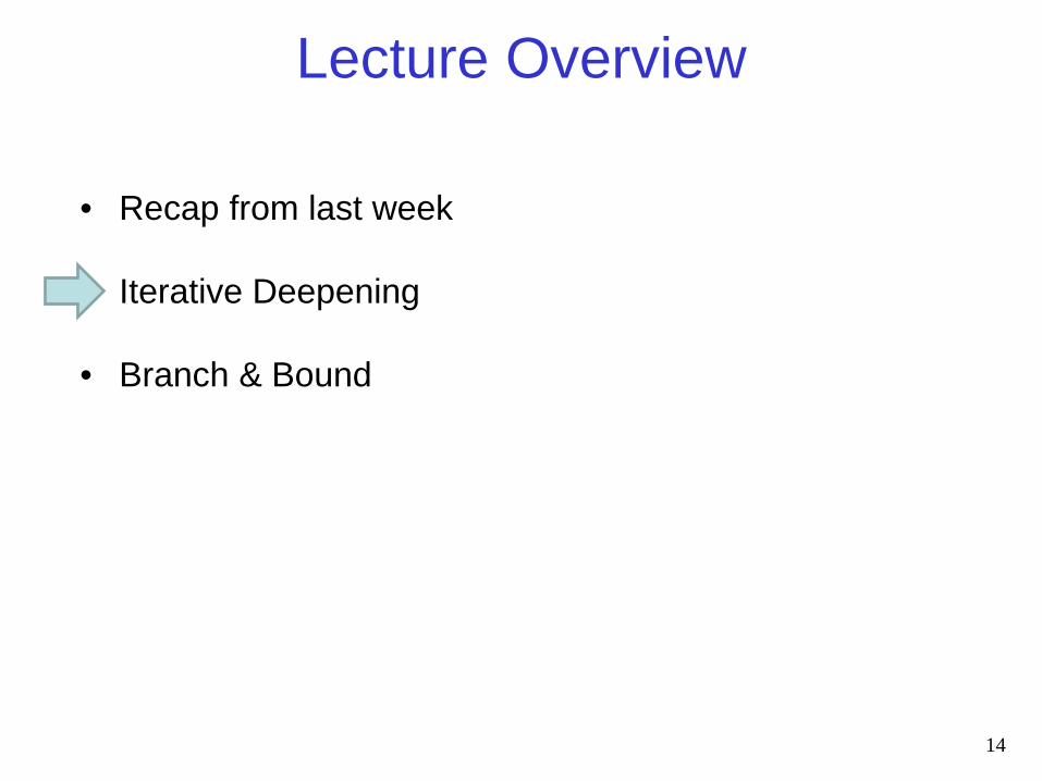
Lecture Overview
• Recap from last week
• Iterative Deepening
• Branch & Bound
Slide 2
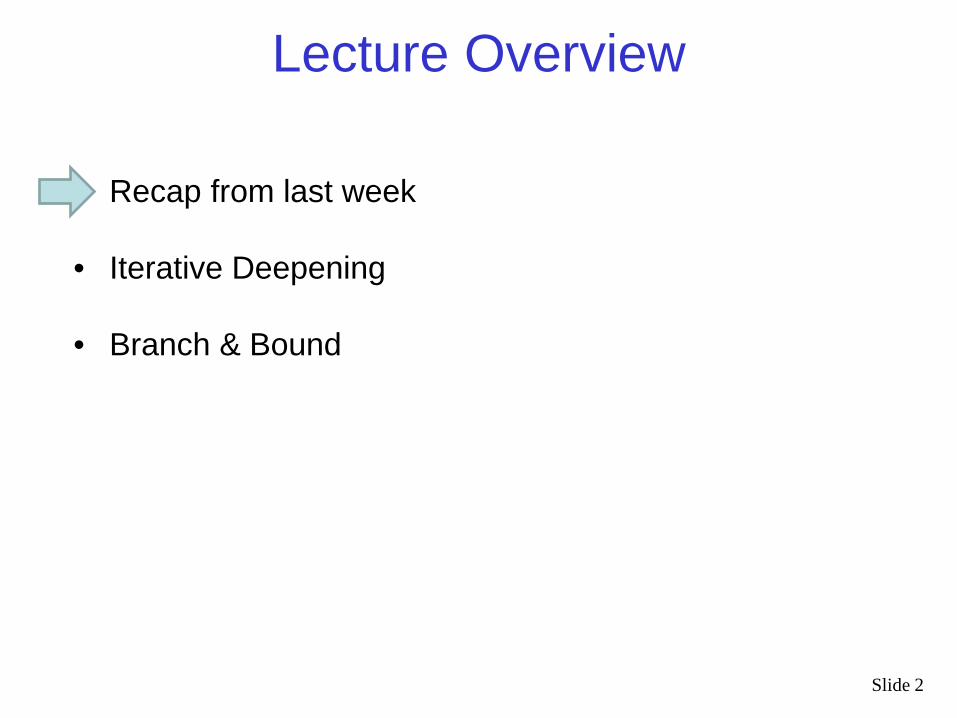
Search with Costs • Sometimes there are costs associated with arcs.
• In this setting we often don't just want to find any solution – we usually want to find the solution that minimizes cost
( ) ),cost(,,cost1
10 ∑=
−=k
iiik nnnn
Def.: The cost of a path is the sum of the costs of its arcs
Def.: A search algorithm is optimal if when it finds a solution, it is the best one: it has the lowest path cost
3
• Expands the path with the lowest cost on the frontier.
• The frontier is implemented as a priority queue ordered
by path cost.
• How does this differ from Dijkstra's algorithm? - The two algorithms are very similar - But Dijkstra’s algorithm
- works with nodes not with paths - stores one bit per node (infeasible for infinite/very large graphs) - checks for cycles
Lowest-Cost-First Search (LCFS)
4
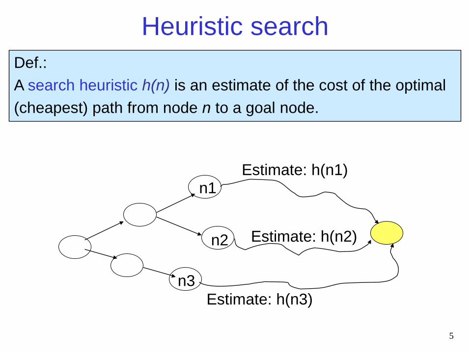
Heuristic search Def.: A search heuristic h(n) is an estimate of the cost of the optimal (cheapest) path from node n to a goal node.
Estimate: h(n1)
5
Estimate: h(n2)
Estimate: h(n3) n3
n2
n1
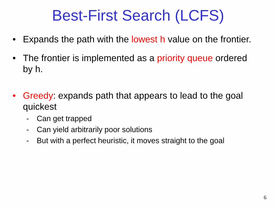
• Expands the path with the lowest h value on the frontier.
• The frontier is implemented as a priority queue ordered
by h.
• Greedy: expands path that appears to lead to the goal quickest - Can get trapped - Can yield arbitrarily poor solutions - But with a perfect heuristic, it moves straight to the goal
Best-First Search (LCFS)
6
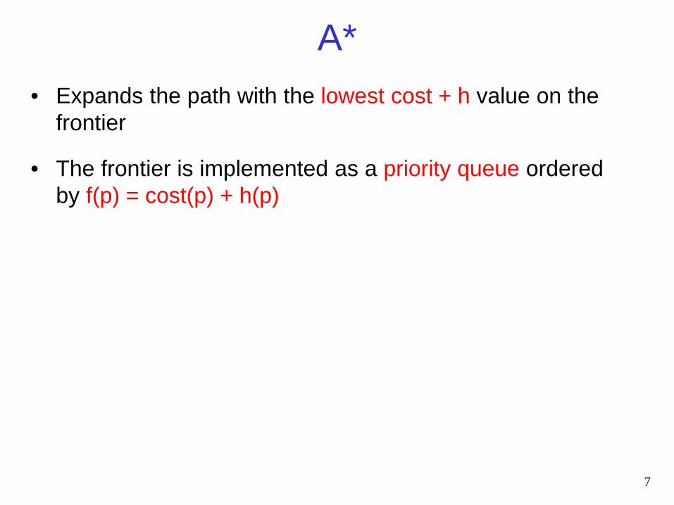
• Expands the path with the lowest cost + h value on the
frontier
• The frontier is implemented as a priority queue ordered by f(p) = cost(p) + h(p)
A*
7
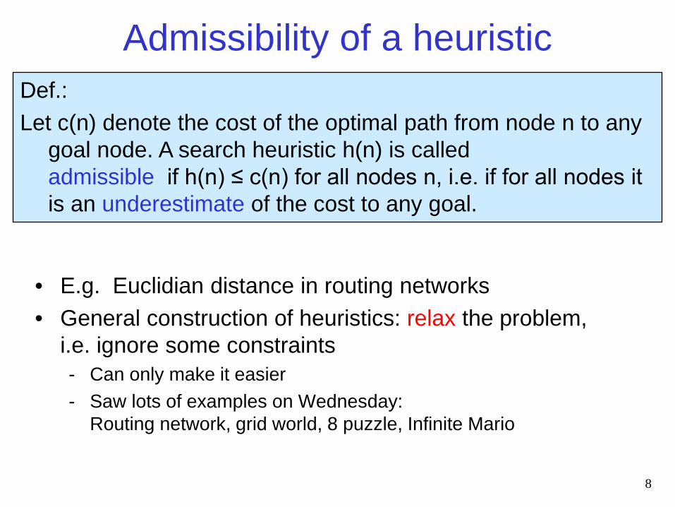
Admissibility of a heuristic
• E.g. Euclidian distance in routing networks • General construction of heuristics: relax the problem,
i.e. ignore some constraints - Can only make it easier - Saw lots of examples on Wednesday:
Routing network, grid world, 8 puzzle, Infinite Mario
8
Def.: Let c(n) denote the cost of the optimal path from node n to any
goal node. A search heuristic h(n) is called admissible if h(n) ≤ c(n) for all nodes n, i.e. if for all nodes it is an underestimate of the cost to any goal.
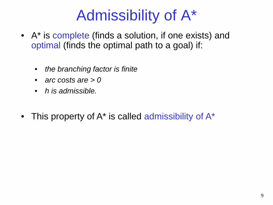
• A* is complete (finds a solution, if one exists) and optimal (finds the optimal path to a goal) if: • the branching factor is finite • arc costs are > 0 • h is admissible.
• This property of A* is called admissibility of A*
Admissibility of A*
9
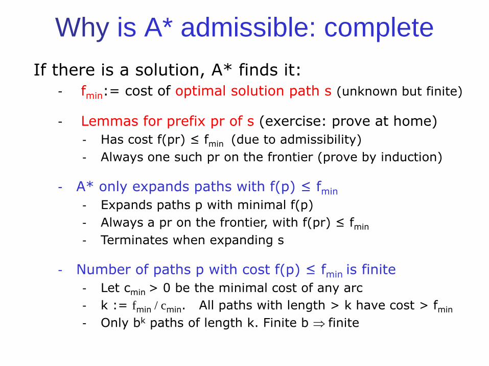
If there is a solution, A* finds it: - fmin:= cost of optimal solution path s (unknown but finite)
- Lemmas for prefix pr of s (exercise: prove at home) - Has cost f(pr) ≤ fmin (due to admissibility) - Always one such pr on the frontier (prove by induction)
- A* only expands paths with f(p) ≤ fmin - Expands paths p with minimal f(p) - Always a pr on the frontier, with f(pr) ≤ fmin - Terminates when expanding s
- Number of paths p with cost f(p) ≤ fmin is finite - Let cmin > 0 be the minimal cost of any arc - k := fmin / cmin. All paths with length > k have cost > fmin - Only bk paths of length k. Finite b ⇒ finite
Why is A* admissible: complete
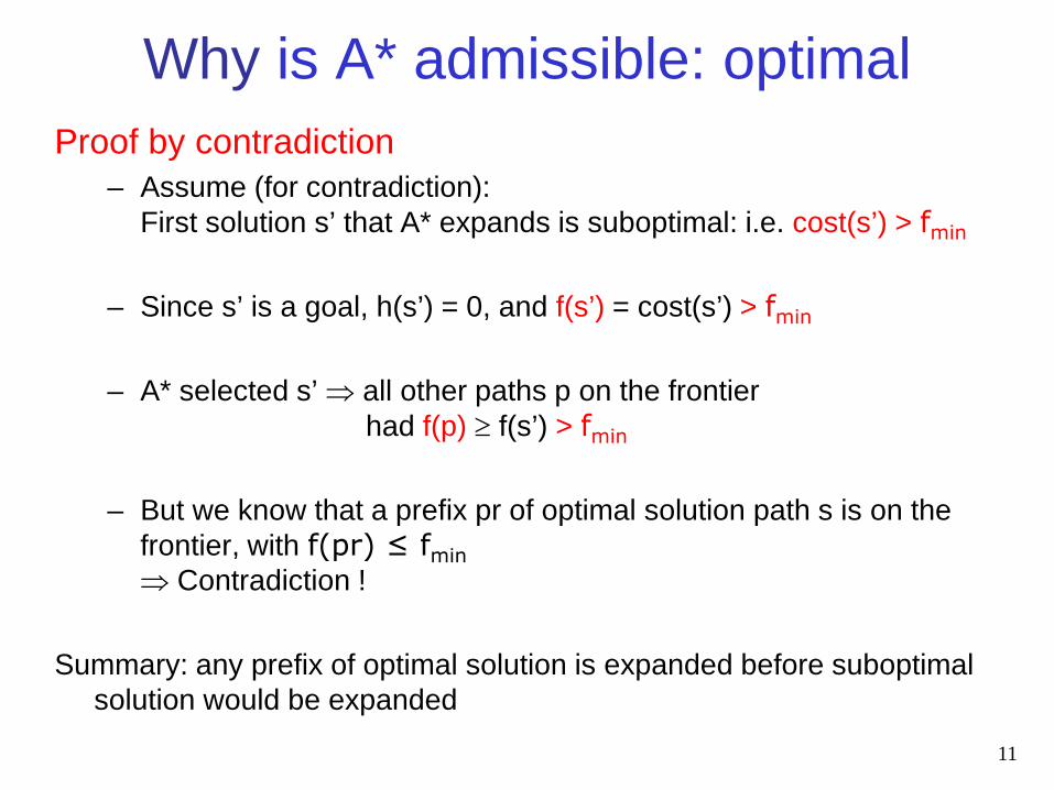
Why is A* admissible: optimal Proof by contradiction
– Assume (for contradiction): First solution s’ that A* expands is suboptimal: i.e. cost(s’) > fmin
– Since s’ is a goal, h(s’) = 0, and f(s’) = cost(s’) > fmin
– A* selected s’ ⇒ all other paths p on the frontier had f(p) ≥ f(s’) > fmin
– But we know that a prefix pr of optimal solution path s is on the frontier, with f(pr) ≤ fmin ⇒ Contradiction !
Summary: any prefix of optimal solution is expanded before suboptimal solution would be expanded
11
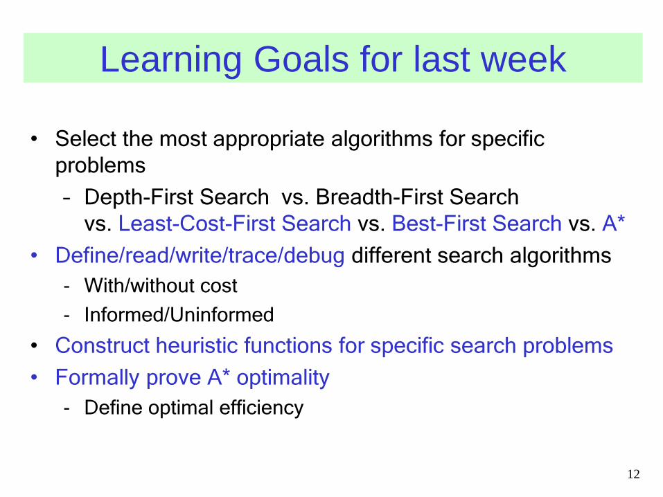
• Select the most appropriate algorithms for specific problems – Depth-First Search vs. Breadth-First Search
vs. Least-Cost-First Search vs. Best-First Search vs. A* • Define/read/write/trace/debug different search algorithms
- With/without cost - Informed/Uninformed
• Construct heuristic functions for specific search problems • Formally prove A* optimality
- Define optimal efficiency
12
Learning Goals for last week
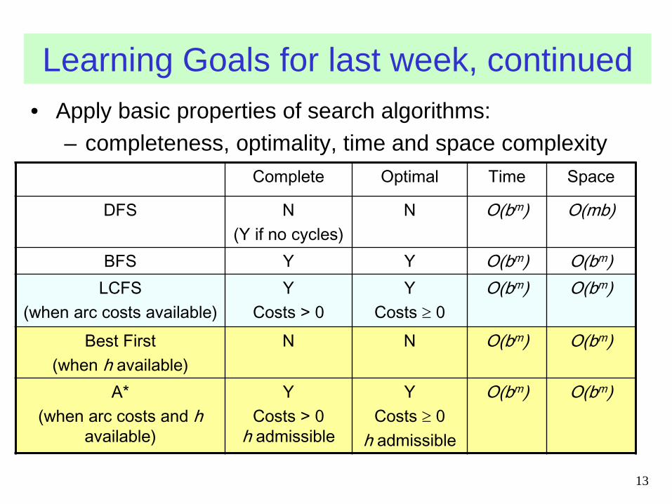
• Apply basic properties of search algorithms: – completeness, optimality, time and space complexity
13
Learning Goals for last week, continued
Complete Optimal Time Space
DFS N (Y if no cycles)
N O(bm) O(mb)
BFS Y Y O(bm) O(bm) LCFS
(when arc costs available) Y
Costs > 0 Y
Costs ≥ 0 O(bm) O(bm)
Best First
(when h available) N N O(bm) O(bm)
A* (when arc costs and h
available)
Y Costs > 0
h admissible
Y Costs ≥ 0
h admissible
O(bm) O(bm)
Lecture Overview
• Recap from last week
• Iterative Deepening
• Branch & Bound
14
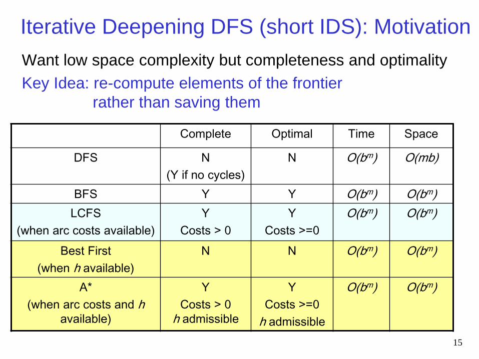
Want low space complexity but completeness and optimality Key Idea: re-compute elements of the frontier
rather than saving them
15
Complete Optimal Time Space
DFS N (Y if no cycles)
N O(bm) O(mb)
BFS Y Y O(bm) O(bm) LCFS
(when arc costs available) Y
Costs > 0 Y
Costs >=0 O(bm) O(bm)
Best First
(when h available) N N O(bm) O(bm)
A* (when arc costs and h
available)
Y Costs > 0
h admissible
Y Costs >=0
h admissible
O(bm) O(bm)
Iterative Deepening DFS (short IDS): Motivation
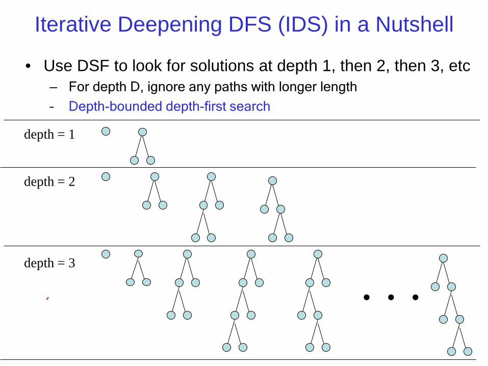
depth = 1 depth = 2 depth = 3
. . .
Iterative Deepening DFS (IDS) in a Nutshell
• Use DSF to look for solutions at depth 1, then 2, then 3, etc – For depth D, ignore any paths with longer length – Depth-bounded depth-first search
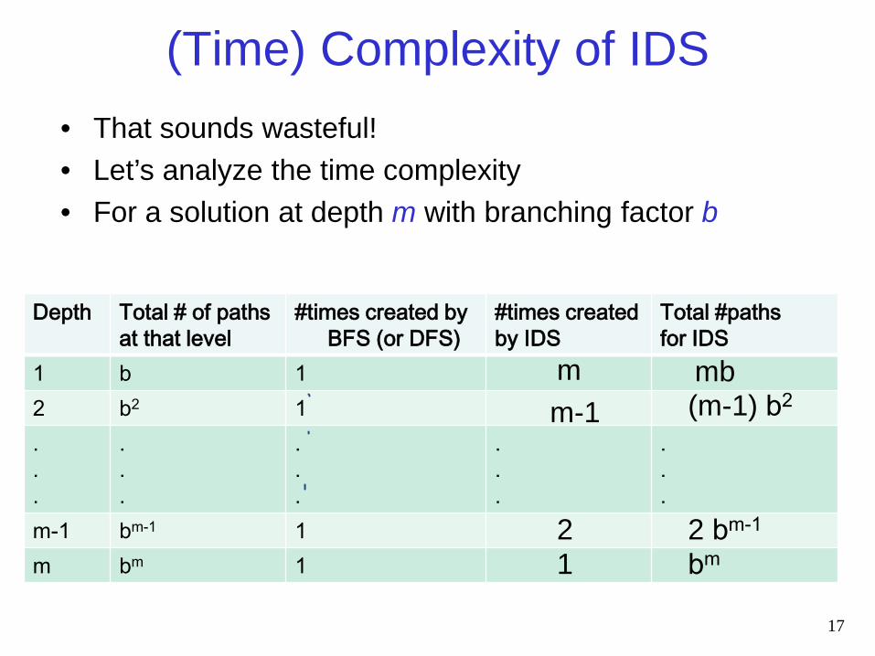
(Time) Complexity of IDS
Depth Total # of paths at that level
#times created by BFS (or DFS)
#times created by IDS
Total #paths for IDS
1 b 1 2 b2 1 . . .
.
.
.
.
.
.
.
.
.
.
.
. m-1 bm-1 1 m bm 1
17
m m-1
2 1
mb (m-1) b2
2 bm-1 bm
• That sounds wasteful! • Let’s analyze the time complexity • For a solution at depth m with branching factor b
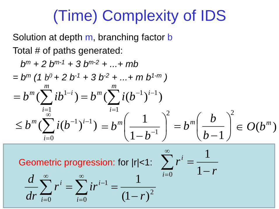
Solution at depth m, branching factor b Total # of paths generated: bm + 2 bm-1 + 3 bm-2 + ...+ mb = bm (1 b0 + 2 b-1 + 3 b-2 + ...+ m b1-m )
))(()(1
11
1
1 ∑∑=
−−
=
− ==m
i
imm
i
im bibibb
(Time) Complexity of IDS
rr
i
i
−=∑
∞
= 11
0 Geometric progression: for |r|<1:
)( mbO∈
20
1
0 )1(1r
irrdrd
i
i
i
i
−==∑∑
∞
=
−∞
=
))((0
11∑∞
=
−−≤i
im bib2
111
−
= −bbm
2
1
−=
bbbm
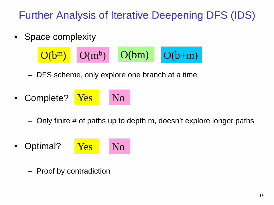
Further Analysis of Iterative Deepening DFS (IDS)
• Space complexity – DFS scheme, only explore one branch at a time
• Complete?
– Only finite # of paths up to depth m, doesn’t explore longer paths
• Optimal?
– Proof by contradiction
19
O(b+m) O(bm) O(bm) O(mb)
Yes No
Yes No
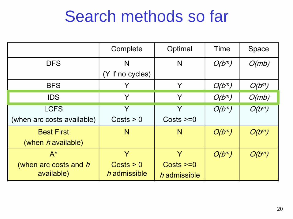
Search methods so far
20
Complete Optimal Time Space
DFS N (Y if no cycles)
N O(bm) O(mb)
BFS Y Y O(bm) O(bm) IDS Y Y O(bm) O(mb)
LCFS (when arc costs available)
Y Costs > 0
Y Costs >=0
O(bm) O(bm)
Best First (when h available)
N N O(bm) O(bm)
A* (when arc costs and h
available)
Y Costs > 0
h admissible
Y Costs >=0
h admissible
O(bm) O(bm)
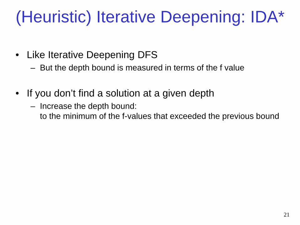
(Heuristic) Iterative Deepening: IDA*
• Like Iterative Deepening DFS – But the depth bound is measured in terms of the f value
• If you don’t find a solution at a given depth – Increase the depth bound:
to the minimum of the f-values that exceeded the previous bound
21
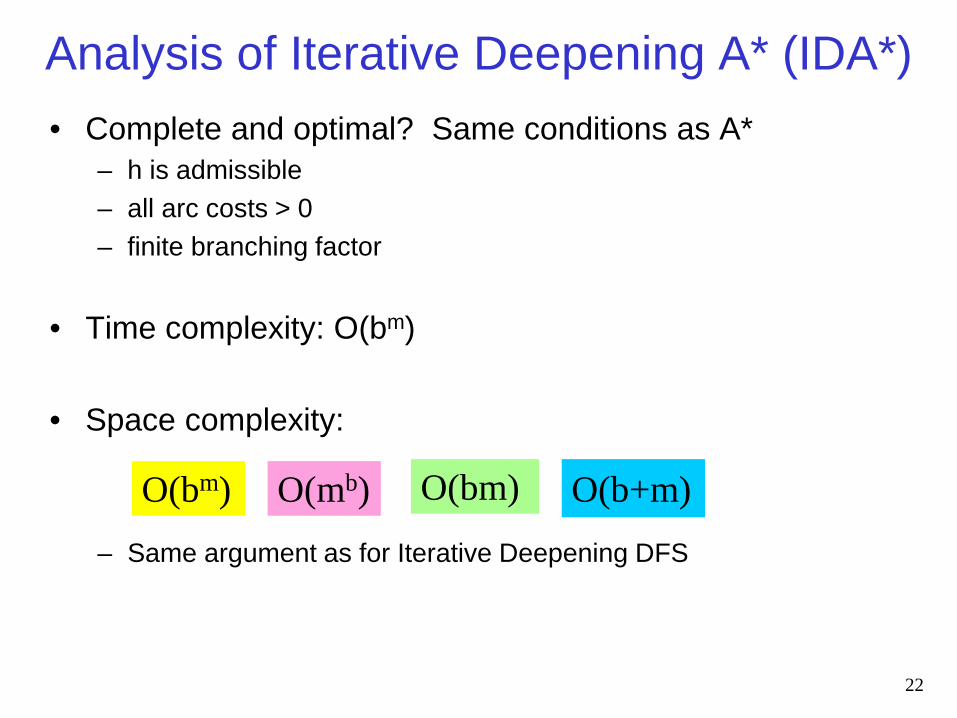
Analysis of Iterative Deepening A* (IDA*) • Complete and optimal? Same conditions as A*
– h is admissible – all arc costs > 0 – finite branching factor
• Time complexity: O(bm)
• Space complexity: – Same argument as for Iterative Deepening DFS
22
O(b+m) O(bm) O(bm) O(mb)
Lecture Overview
• Recap from last week
• Iterative Deepening
• Branch & Bound
23
Heuristic DFS • Other than IDA*, can we use heuristic information in DFS?
– When we expand a node, put all its neighbours on the stack – In which order?
• Can use heuristic guidance: h or f • Perfect heuristic: would solve problem without any backtracking
• Heuristic DFS is very frequently used in practice
– Often don’t need optimal solution, just some solution – No requirement for admissibility of heuristic
• As long as we don’t end up in infinite paths
24
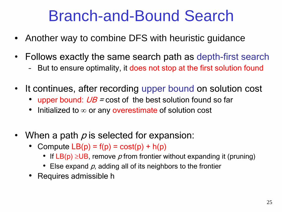
Branch-and-Bound Search • Another way to combine DFS with heuristic guidance
• Follows exactly the same search path as depth-first search – But to ensure optimality, it does not stop at the first solution found
• It continues, after recording upper bound on solution cost • upper bound: UB = cost of the best solution found so far • Initialized to ∞ or any overestimate of solution cost
• When a path p is selected for expansion:
• Compute LB(p) = f(p) = cost(p) + h(p) • If LB(p) ≥UB, remove p from frontier without expanding it (pruning)
• Else expand p, adding all of its neighbors to the frontier • Requires admissible h
25
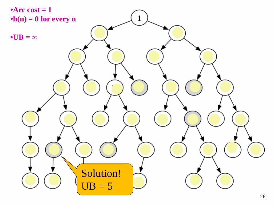
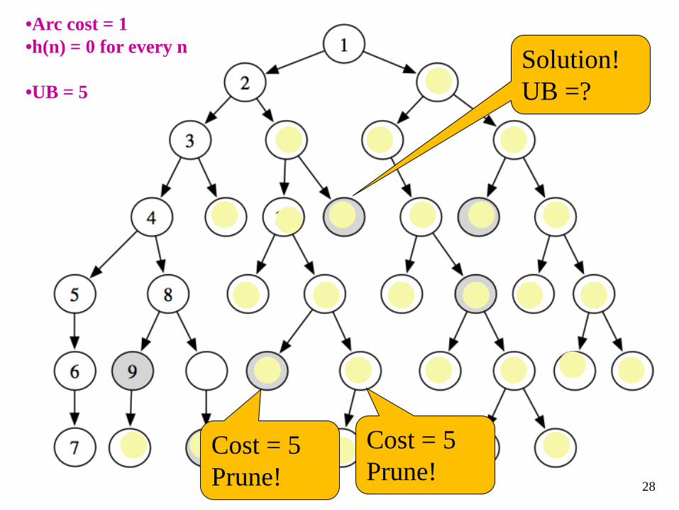
Example •Arc cost = 1 •h(n) = 0 for every n
•UB = ∞
Solution! UB = ?
26
Solution! UB = 5
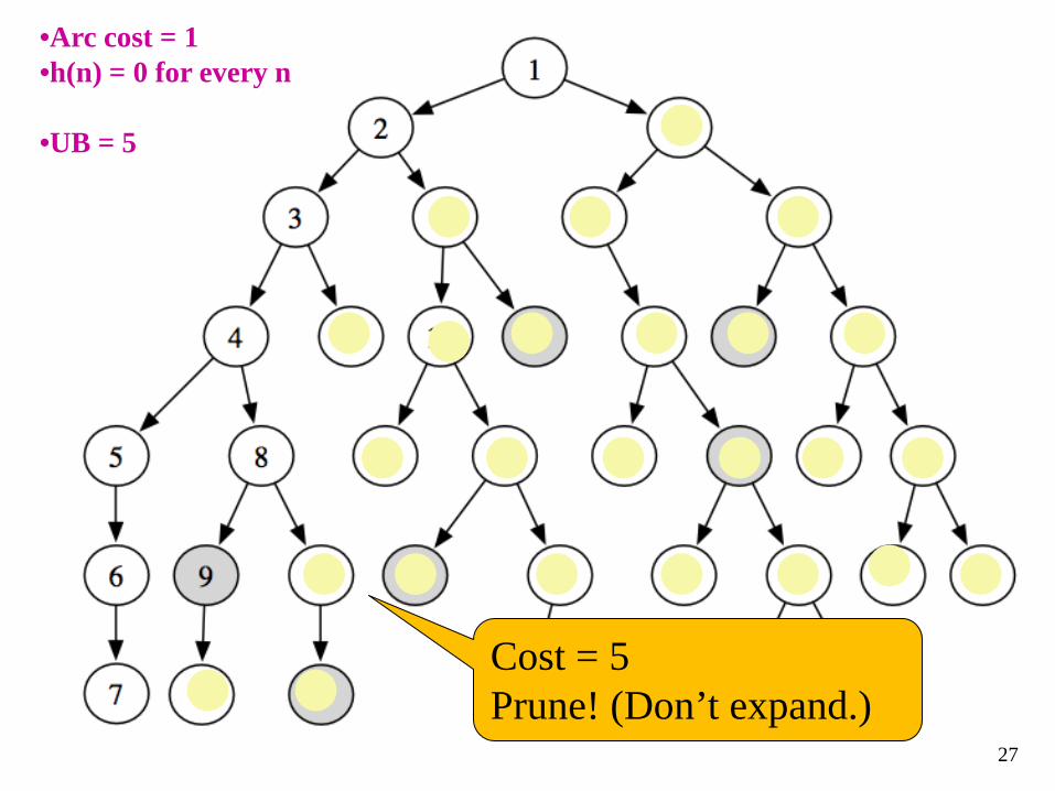
Example •Arc cost = 1 •h(n) = 0 for every n
•UB = 5
Cost = 5 Prune! (Don’t expand.)
27
Example •Arc cost = 1 •h(n) = 0 for every n
•UB = 5
Cost = 5 Prune!
Cost = 5 Prune!
Solution! UB =?
28
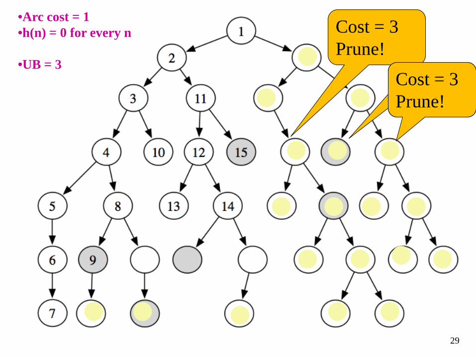
Example •Arc cost = 1 •h(n) = 0 for every n
•UB = 3
Cost = 3 Prune!
Cost = 3 Prune!
29
Cost = 3 Prune!
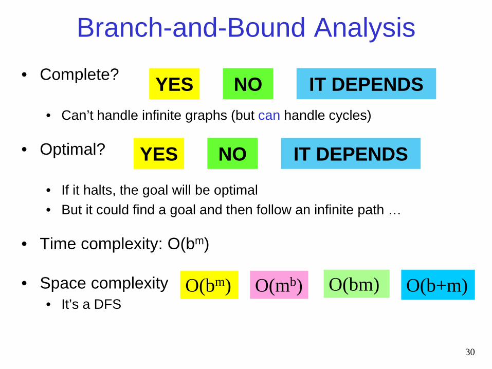
Branch-and-Bound Analysis • Complete?
• Can’t handle infinite graphs (but can handle cycles)
• Optimal? • If it halts, the goal will be optimal • But it could find a goal and then follow an infinite path …
• Time complexity: O(bm)
• Space complexity • It’s a DFS
NO IT DEPENDS YES
30
NO IT DEPENDS YES
O(b+m) O(bm) O(bm) O(mb)
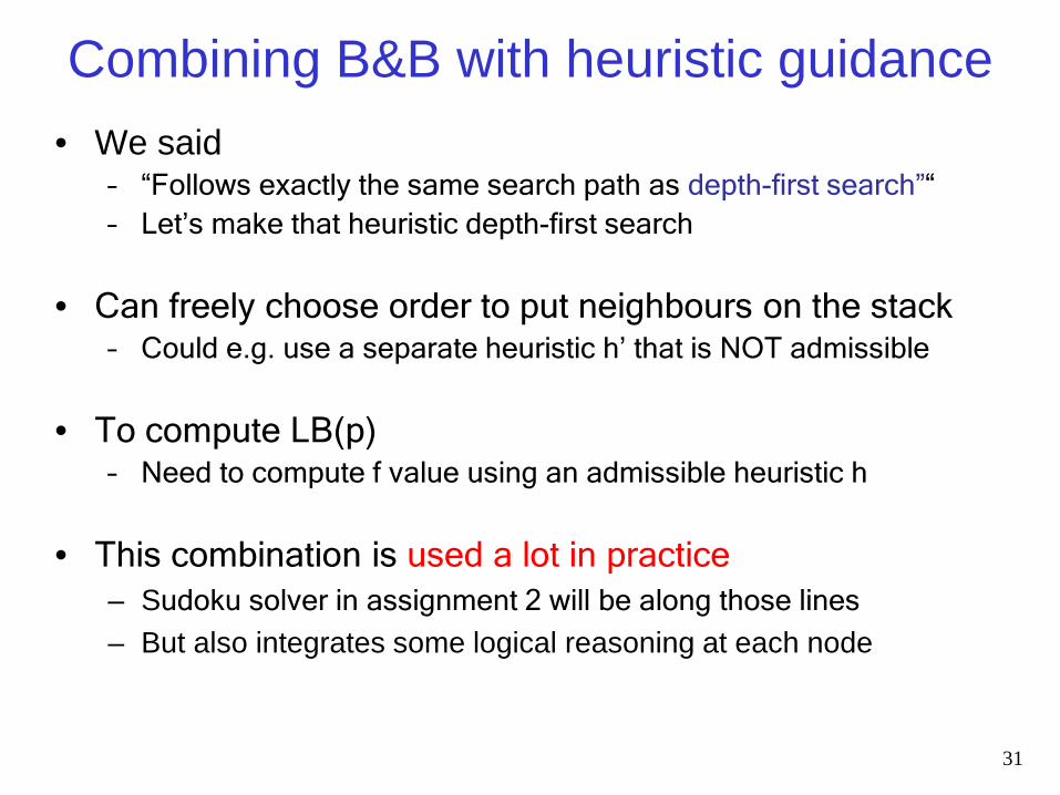
Combining B&B with heuristic guidance • We said
– “Follows exactly the same search path as depth-first search”“ – Let’s make that heuristic depth-first search
• Can freely choose order to put neighbours on the stack – Could e.g. use a separate heuristic h’ that is NOT admissible
• To compute LB(p) – Need to compute f value using an admissible heuristic h
• This combination is used a lot in practice – Sudoku solver in assignment 2 will be along those lines – But also integrates some logical reasoning at each node
31
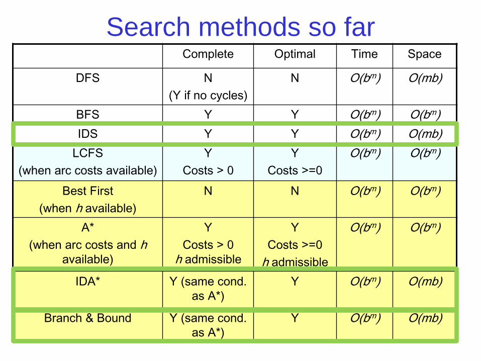
Search methods so far Complete Optimal Time Space
DFS N (Y if no cycles)
N O(bm) O(mb)
BFS Y Y O(bm) O(bm) IDS Y Y O(bm) O(mb)
LCFS (when arc costs available)
Y Costs > 0
Y Costs >=0
O(bm) O(bm)
Best First (when h available)
N N O(bm) O(bm)
A* (when arc costs and h
available)
Y Costs > 0
h admissible
Y Costs >=0
h admissible
O(bm) O(bm)
IDA* Y (same cond. as A*)
Y O(bm)
O(mb)
Branch & Bound Y (same cond. as A*)
Y O(bm) O(mb)
33
Memory-bounded A*
• Iterative deepening A* and B & B use little memory • What if we've got more memory, but not O(bm)? • Do A* and keep as much of the frontier in memory as
possible • When running out of memory
• delete worst path (highest f value) from frontier • Back its f value up to a common ancestor
• Subtree gets regenerated only when all other paths have been shown to be worse than the “forgotten” path
• Details are beyond the scope of the course, but • Complete and optimal if solution is at depth manageable for
available memory
• Define/read/write/trace/debug different search algorithms - New: Iterative Deepening,
Iterative Deepening A*, Branch & Bound
• Apply basic properties of search algorithms: – completeness, optimality, time and space complexity
Announcements:
– New practice exercises are out: see WebCT • Heuristic search • Branch & Bound • Please use these! (Only takes 5 min. if you understood things…)
– Assignment 1 is out: see WebCT
34
Learning Goals for today’s class