University of IowaIowa Research Online

Theses and Dissertations

Summer 2010

A biomechanical model of femoral forces duringfunctional electrical stimulation after spinal cordinjury in supine and seated positionsColleen Louise McHenryUniversity of Iowa

Copyright 2010 Colleen Louise McHenry

This thesis is available at Iowa Research Online: http://ir.uiowa.edu/etd/710

Follow this and additional works at: http://ir.uiowa.edu/etd

Part of the Biomedical Engineering and Bioengineering Commons

Recommended CitationMcHenry, Colleen Louise. "A biomechanical model of femoral forces during functional electrical stimulation after spinal cord injury insupine and seated positions." MS (Master of Science) thesis, University of Iowa, 2010.http://ir.uiowa.edu/etd/710.

1

A BIOMECHANICAL MODEL OF FEMORAL FORCES DURING

FUNCTIONAL ELECTRICAL STIMULATION AFTER SPINAL

CORD INJURY IN SUPINE AND SEATED POSITIONS

by

Colleen Louise McHenry

A thesis submitted in partial fulfillment of the requirements for the Master of

Science degree in Biomedical Engineering in the Graduate College of

The University of Iowa

July 2010

Thesis Supervisors: Professor Richard K. Shields

Associate Professor Nicole M. Grosland

Copyright by COLLEEN LOUISE MCHENRY

2010 All Rights Reserved

Graduate College The University of Iowa

Iowa City, Iowa

CERTIFICATE OF APPROVAL

_______________________

MASTER'S THESIS

_______________

This is to certify that the Master's thesis of

Colleen Louise McHenry

has been approved by the Examining Committee for the thesis requirement for the Master of Science degree in Biomedical

Engineering at the July 2010 graduation.

Thesis Committee: ___________________________________ Nicole M. Grosland, Thesis Supervisor

___________________________________ Richard K. Shields, Thesis Supervisor

___________________________________ Tae-Hong Lim

ii

4

ACKNOWLEDGMENTS

First, I would like to thank the Neuromuscular Lab in the Physical Therapy and

Rehabilitation Science department. I not only completed my master’s thesis in their lab,

but also was inspired to continue my education in this department. My advisor, Dr.

Richard Shields, has guided my throughout this project and has prompted questions

which encouraged independent thought. My lab mates, Andy and Shauna, have mentored

me and offered their expertise throughout the project. Shauna has been there to critically

examine my rationale and my findings which led me to build stronger arguments and not

settle with the first attempt. I also want to thank the Biomedical Engineering department

for teaching me the critical thinking and problem solving skills required to complete my

master’s thesis especially my academic advisor, Dr. Nicole Grosland.

I also need to recognize and thank those who have personally supported me

throughout this process. My parents, Mark and Michelle McHenry, fostered an

environment conducive to learning and academic success. They promoted analytical

thinking and creativity in a loving, warm home. My sisters, Molly and Emily, and my

brother, Jonathan, have been there to offer words of encouragement and to make me

laugh. I would also like to thank the many friends that have supported me during this

process, especially Mike for giving his time and troubleshooting skills. Finally, I would

like to thank my friend and roommate, Cassie, for always listening and motivating me to

complete this project. Throughout these two years, she has been there to offer a warm

meal and much needed words of encouragement. I would not have been able to finish this

project without all of these wonderful individuals.

iii

ABSTRACT

Following a spinal cord injury (SCI), the paralyzed extremities undergo muscle

atrophy and decrease in bone mineral density (BMD) due in part to the loss of

physiological loading. It is crucial to prevent musculoskeletal deterioration so the

population is less susceptible to fractures, and could take advantage of stem cell treatment

if it becomes available. Functional electrical stimulation (FES) has been shown to

advantageously train the paralyzed extremities. However, there is a risk of fracture during

FES due to low BMD of individuals with SCI. Therefore, the forces generated during

FES need to be modeled so researchers and clinicians safely administer this intervention.

The purpose of this project was to develop a biomechanical or mathematical

model to estimate the internal compressive and shear forces at the distal femur, a

common fracture site for individuals with SCI during FES. Therefore, a two-dimensional

static model was created of the lower extremity in the supine and seated positions. The

compressive and shear forces at the distal femur were estimated for both positions during

FES. These internal compressive and shear forces estimated at the distal femur by the

supine model were compared to those estimated by the standing model. Also, for the

seated model, the compressive and shear forces at the distal femur estimated by a tetanic

muscle contraction were compared to those estimated by a doublet muscle contraction.

Finally, the supine model was validated using experimental testing.

The primary findings are 1) the standing model estimated more compressive force

and less shear force at the distal femur compared to the supine model when position and

quadriceps muscle force remain constant and 2) for the seated model, a tetanic quadriceps

muscle contraction predicts greater compressive and shear at the distal femur compared

to a doublet muscle contraction. Also the validation testing revealed a 3.4% error

between the supine model and the experimental testing. These models provide valuable

insights into the internal forces at the distal femur during FES for those with SCI.

iv

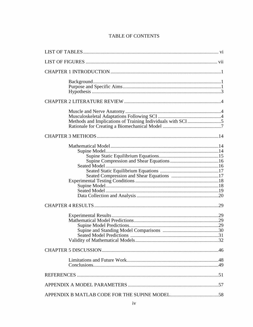
TABLE OF CONTENTS

LIST OF TABLES ............................................................................................................. vi

LIST OF FIGURES .......................................................................................................... vii

CHAPTER 1 INTRODUCTION .........................................................................................1

Background .......................................................................................................1 Purpose and Specific Aims ...............................................................................1 Hypothesis ........................................................................................................3

CHAPTER 2 LITERATURE REVIEW ..............................................................................4

Muscle and Nerve Anatomy .............................................................................4 Musculoskeletal Adaptations Following SCI ...................................................4 Methods and Implications of Training Individuals with SCI ...........................5 Rationale for Creating a Biomechanical Model ...............................................7

CHAPTER 3 METHODS ..................................................................................................14

Mathematical Model .......................................................................................14 Supine Model ...........................................................................................14 Supine Static Equilibrium Equations ................................................15 Supine Compression and Shear Equations .......................................16 Seated Model ...........................................................................................16 Seated Static Equilibrium Equations ...............................................17 Seated Compression and Shear Equations ......................................17

Experimental Testing Conditions ...................................................................18 Supine Model ...........................................................................................18 Seated Model ...........................................................................................19 Data Collection and Analysis ..................................................................20

CHAPTER 4 RESULTS ....................................................................................................29

Experimental Results ......................................................................................29 Mathematical Model Predictions ....................................................................29

Supine Model Predictions ........................................................................29 Supine and Standing Model Comparisons .............................................30 Seated Model Predictions .......................................................................31

Validity of Mathematical Models ...................................................................32

CHAPTER 5 DISCUSSION ..............................................................................................46

Limitations and Future Work..........................................................................48 Conclusions.....................................................................................................49

REFERENCES ..................................................................................................................51

APPENDIX A MODEL PARAMETERS .........................................................................57

APPENDIX B MATLAB CODE FOR THE SUPINE MODEL.......................................58

v

APPENDIX C MATLAB CODE FOR THE SEATED MODEL .....................................61

vi

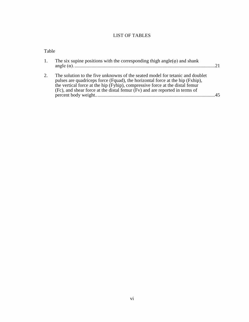
LIST OF TABLES

Table

1. The six supine positions with the corresponding thigh angle(φ) and shank angle (α). ...................................................................................................................21

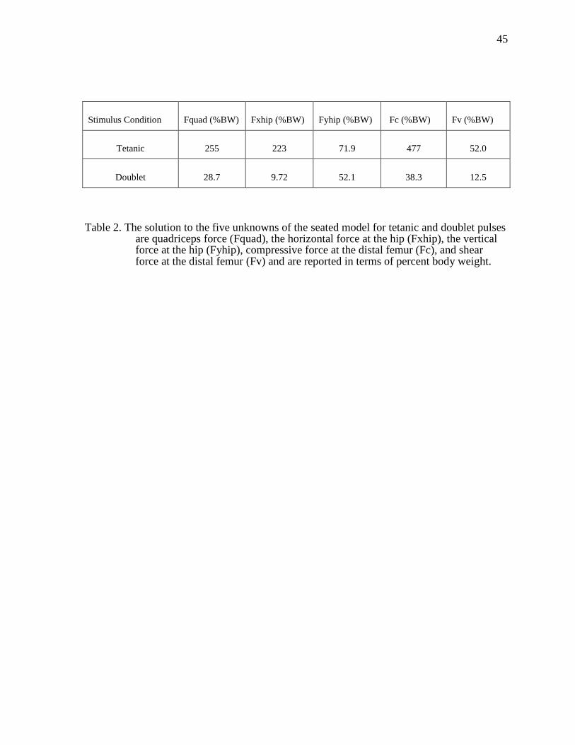
2. The solution to the five unknowns of the seated model for tetanic and doublet pulses are quadriceps force (Fquad), the horizontal force at the hip (Fxhip), the vertical force at the hip (Fyhip), compressive force at the distal femur (Fc), and shear force at the distal femur (Fv) and are reported in terms of percent body weight.. ................................................................................................45

vii

FIGURES

Figure

1. Schematic free body diagram of the lower body during (A) passive stance and (B) active (no added resistance, R=0) and/or active-resistive stance (R = 16.7-67.7% BW). The internal forces from the quadriceps and patellar tendons (Fquad and Fpat, respectively) in B) replace the Fpad in (A) ..................................10

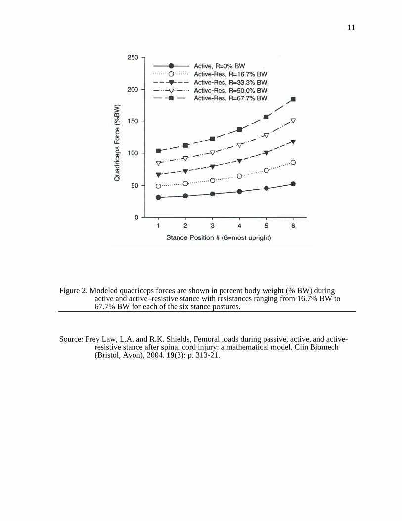
2. Modeled quadriceps forces are shown in percent body weight (% BW) during active and active–resistive stance with resistances ranging from 16.7% BW to 67.7% BW for each of the six stance postures .........................................................11

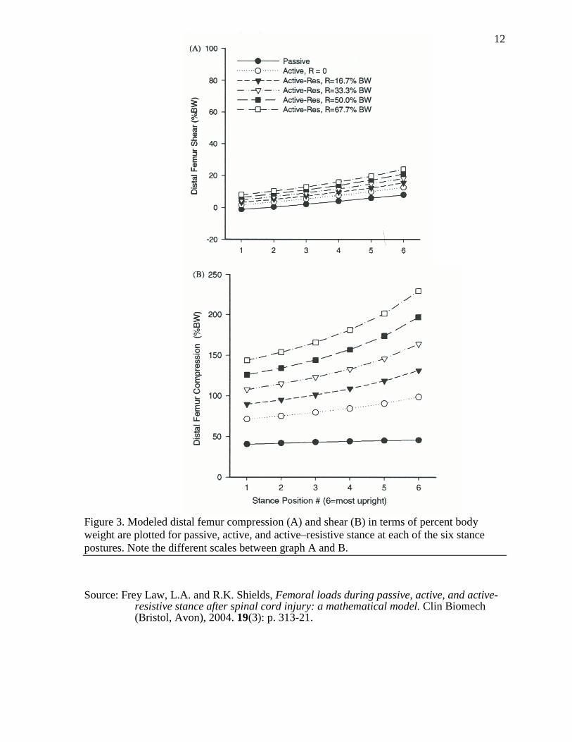
3. Modeled distal femur compression (A) and shear (B) in terms of percent body weight are plotted for passive, active, and active–resistive stance at each of the six stance postures. Note the different scales between graph A and B. .............12

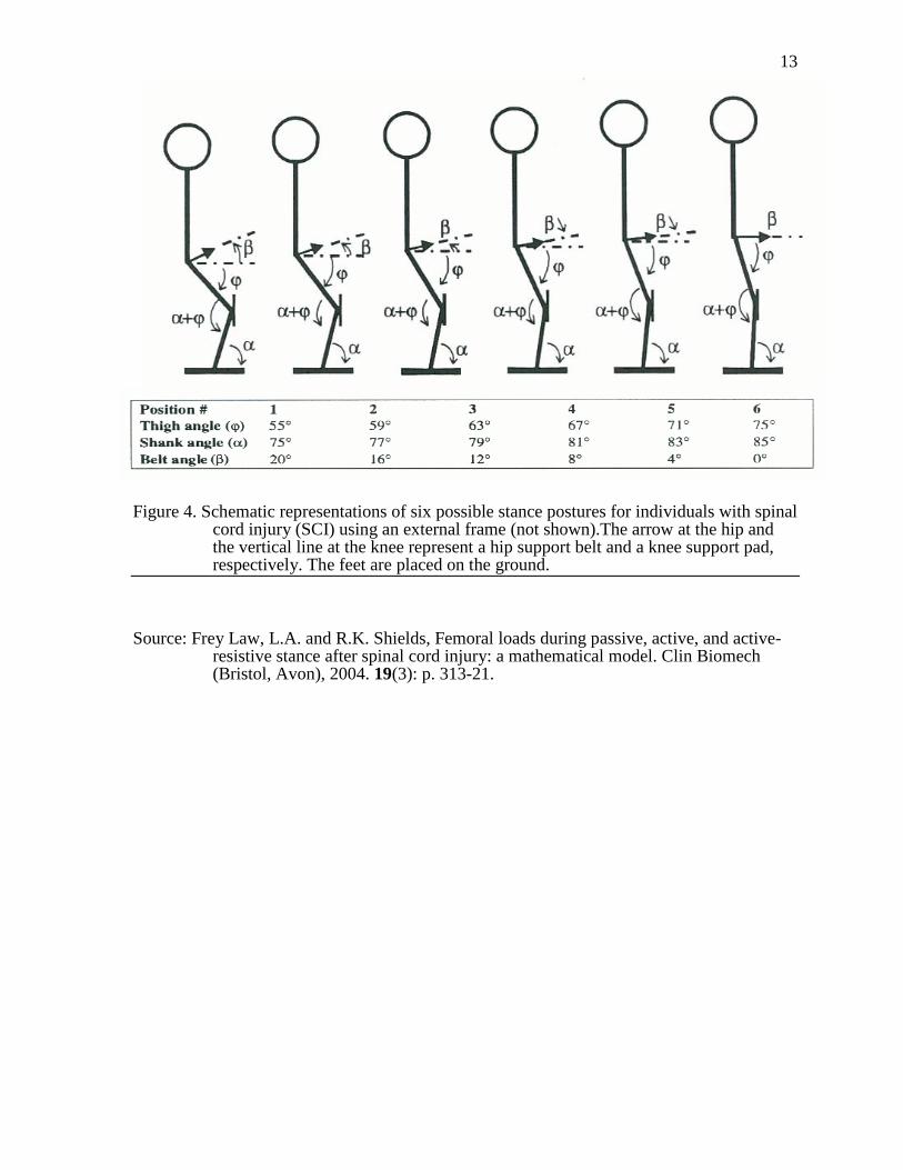
4. Schematic representations of six possible stance postures for individuals with spinal cord injury (SCI) using an external frame (not shown).The arrow at the hip and the vertical line at the knee represent a hip support belt and a knee support pad, respectively. The feet are placed on the ground...................................13

5. Schematic free body diagram of the external forces and loading conditions acting on the lower extremity for the supine model .................................................21

6. Schematic representation of the relationship between the quadriceps tendon or muscle (Fquad) and the patellar tendon (Fpat) at the knee joint. ............................22

7. Schematic free body diagram of the distal femur for the supine model which has been cut at 85% of thigh segment length from the hip joint. The bending moment at the distal femur was not determined but the compressive force (Fc) and shear force (Fv) were calculated. ..............................................................23

8. Schematic free body diagram of the external forces and loading conditions acting on the lower extremity for the seated model ..................................................24

9. Schematic free body diagram of the distal femur for the seated model which has been cut at 85% of thigh segment length from the hip joint. The bending moment at the distal femur was not determined but the compressive force (Fc) and shear force (Fv) were calculated. ...............................................................25

10. Placement of surface electrodes over the quadriceps muscle ...................................26

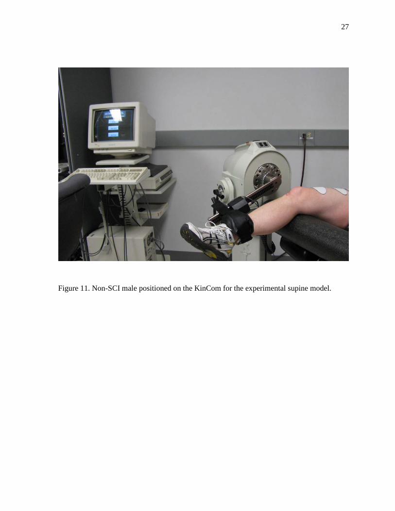
11. Non-SCI male positioned on the KinCom for the experimental supine model ........27

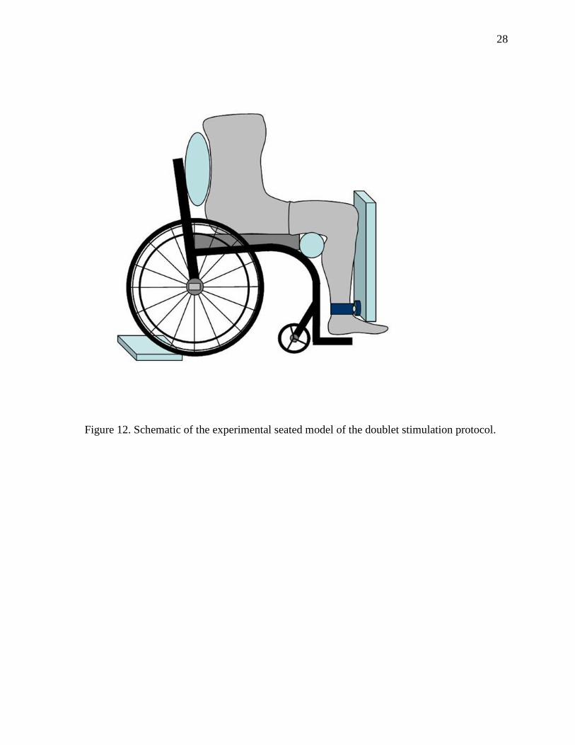
12. Schematic of the experimental seated model of the doublet stimulation protocol .....................................................................................................................28

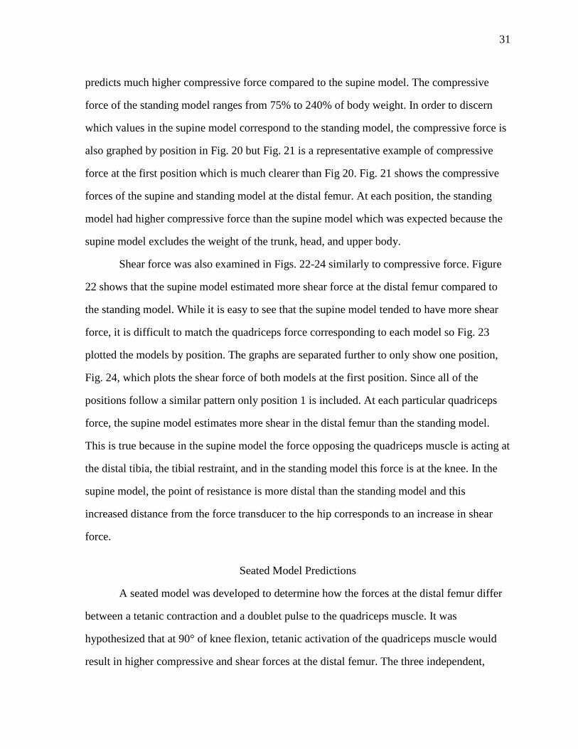
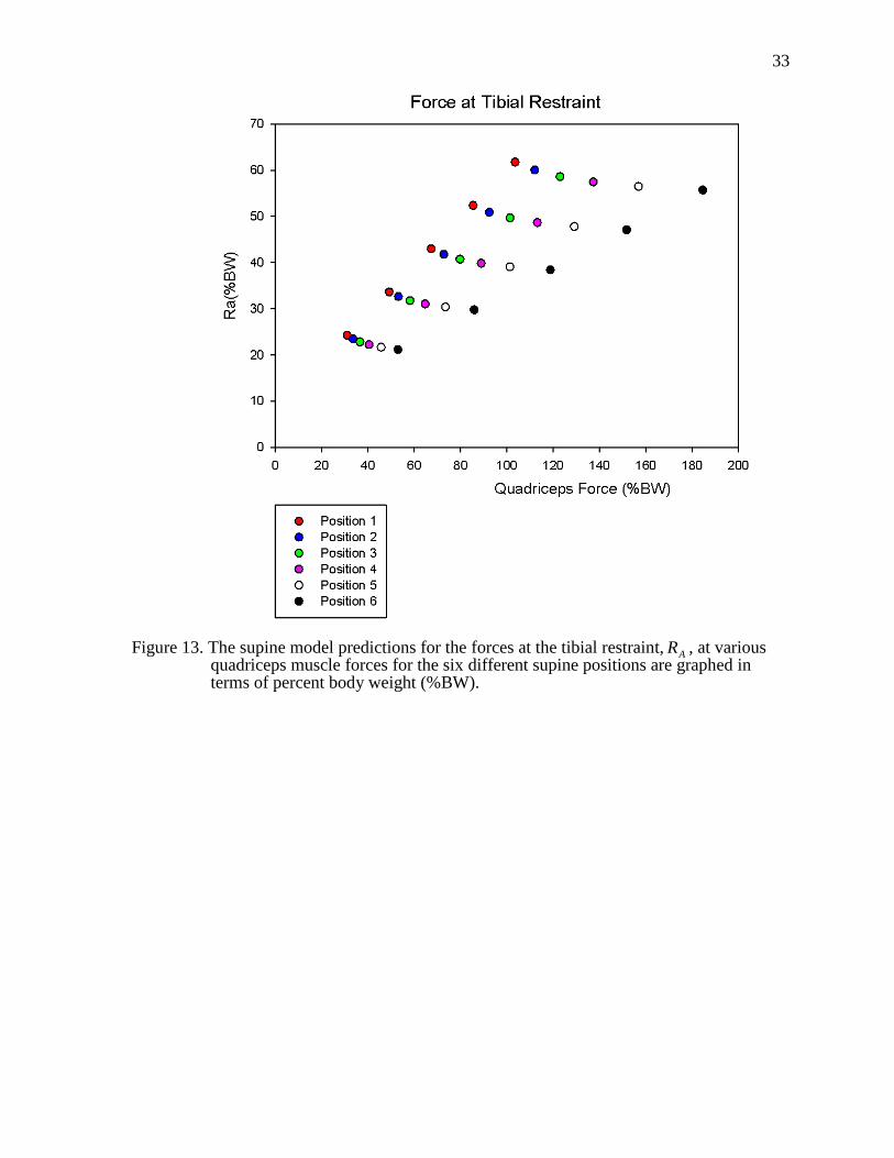
13. The supine model predictions for the forces at the tibial restraint, AR , at various quadriceps muscle forces for the six different supine positions are graphed in terms of percent body weight (%BW). ..................................................33

viii

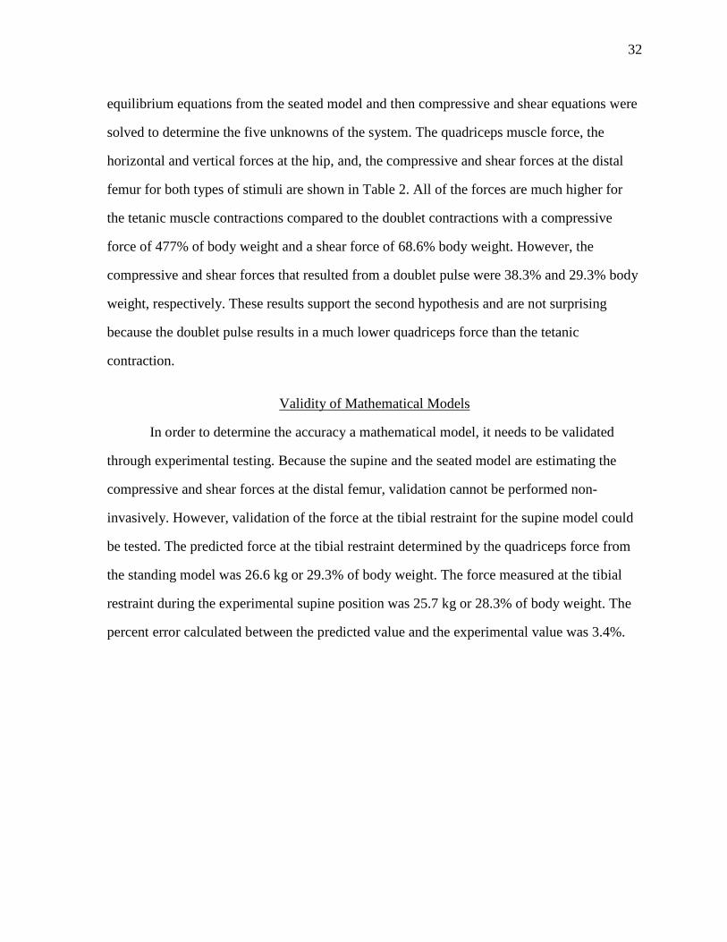
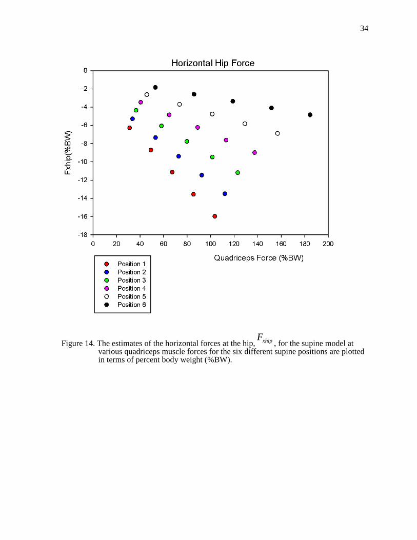
14. The estimates of the horizontal forces at the hip, Fxhip, for the supine model at various quadriceps muscle forces for the six different supine positions are plotted in terms of percent body weight (%BW). .....................................................34

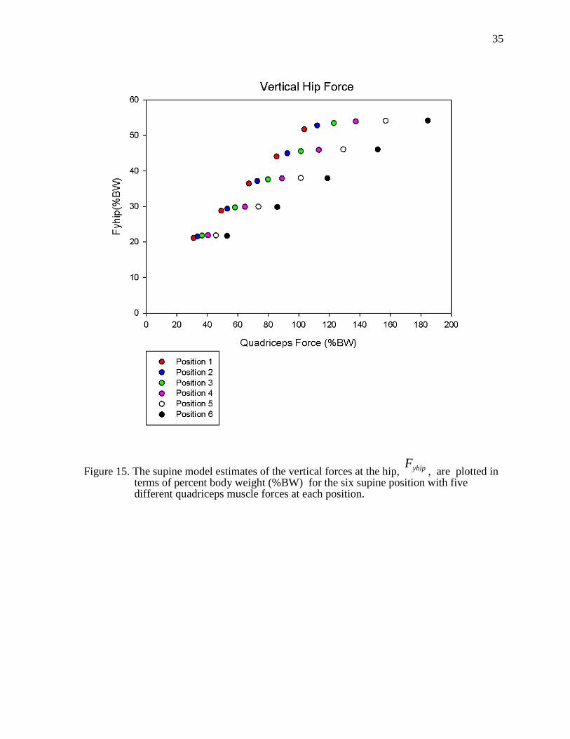
15. The supine model estimates of the horizontal forces at the hip, Fyhip, are plotted in terms of percent body weight (%BW) for the six supine position with five different quadriceps muscle forces at each position. .................................35

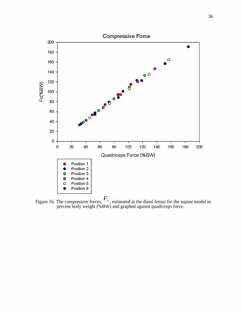
16. The compressive forces, Fc , estimated at the distal femur for the supine model in percent body weight (%BW) and graphed against quadriceps force. ........36

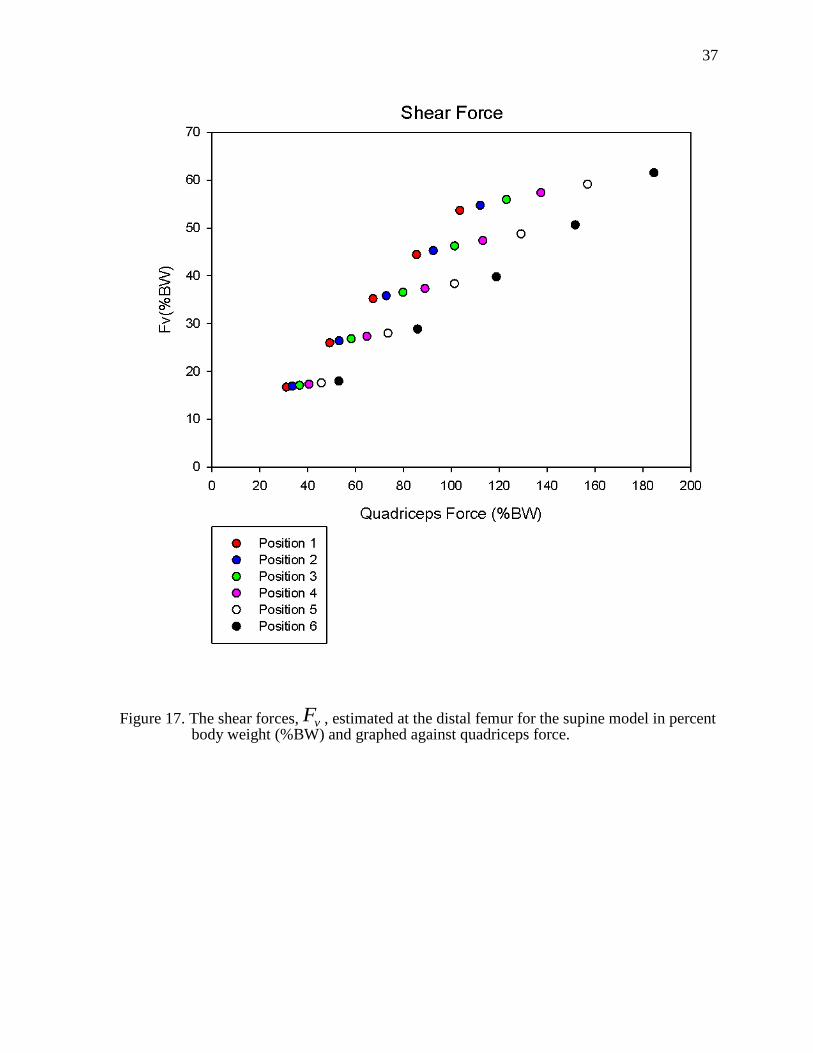
17. The shear forces, Fv, estimated at the distal femur for the supine model in percent body weight (%BW) and graphed against quadriceps force. .......................37

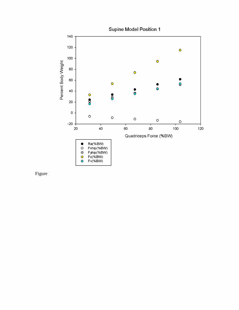
18. The estimates from the supine model for the tibial restraint force, the horizontal and vertical forces at the hip, and the compressive and shear forces at the distal femur for position 1 at five quadriceps forces .......................................38

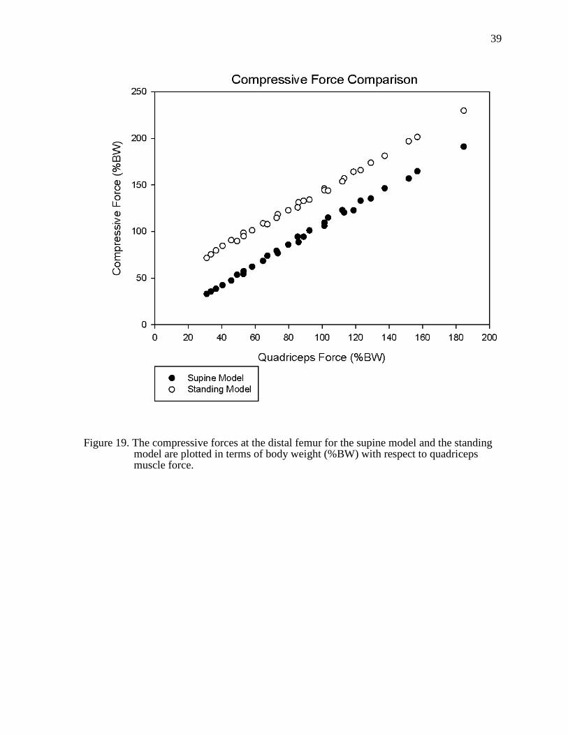
19. The compressive forces at the distal femur for the supine model and the standing model are plotted in terms of body weight (%BW) with respect to quadriceps muscle force............................................................................................39

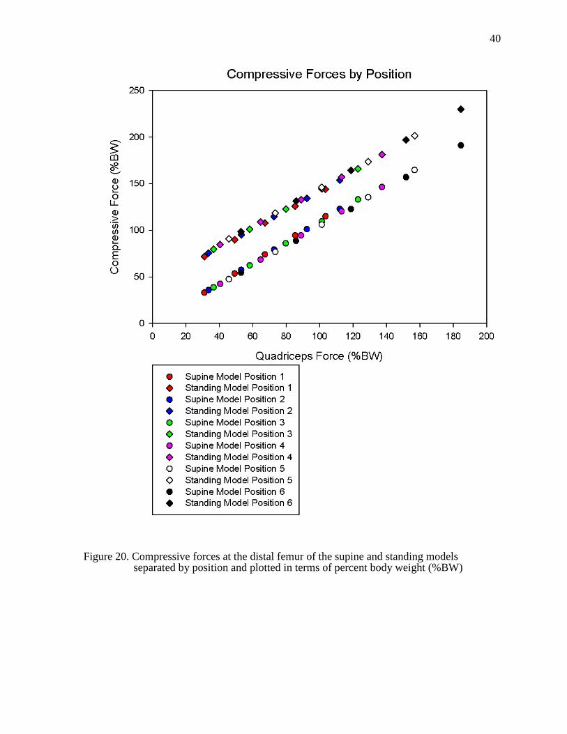
20. Compressive forces at the distal femur of the supine and standing models separated by position and plotted in terms of percent body weight (%BW) ...........40

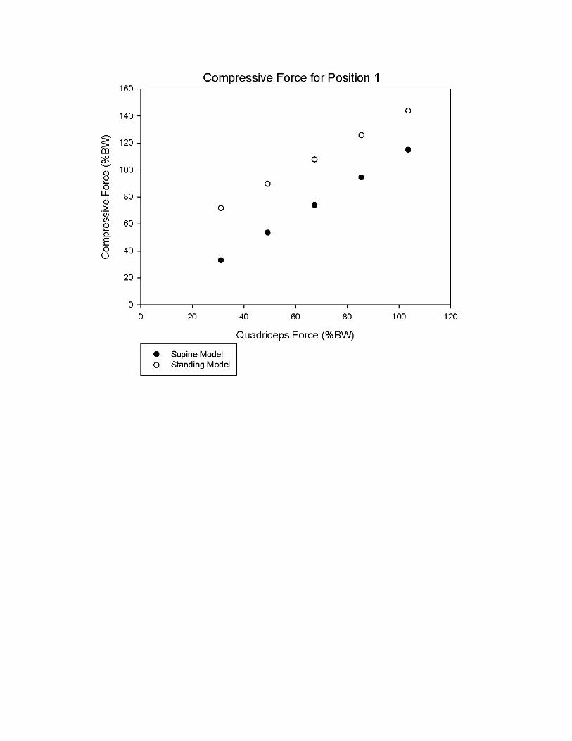
21. A representative example of the compressive forces at the distal femur of position 1 for the supine and standing models as a percent of body weight (%BW) plotted against quadriceps muscle force ......................................................41

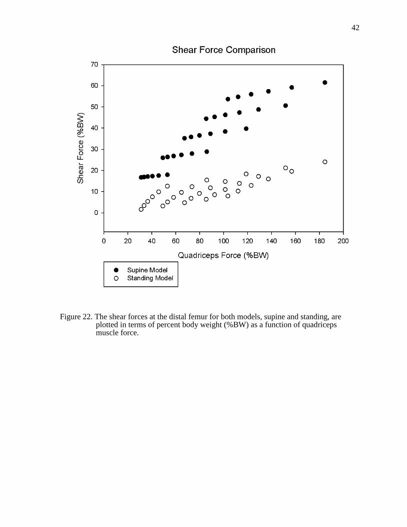
22. The shear forces at the distal femur for both models, supine and standing, are plotted in terms of percent body weight (%BW) as a function of quadriceps muscle force ..............................................................................................................42

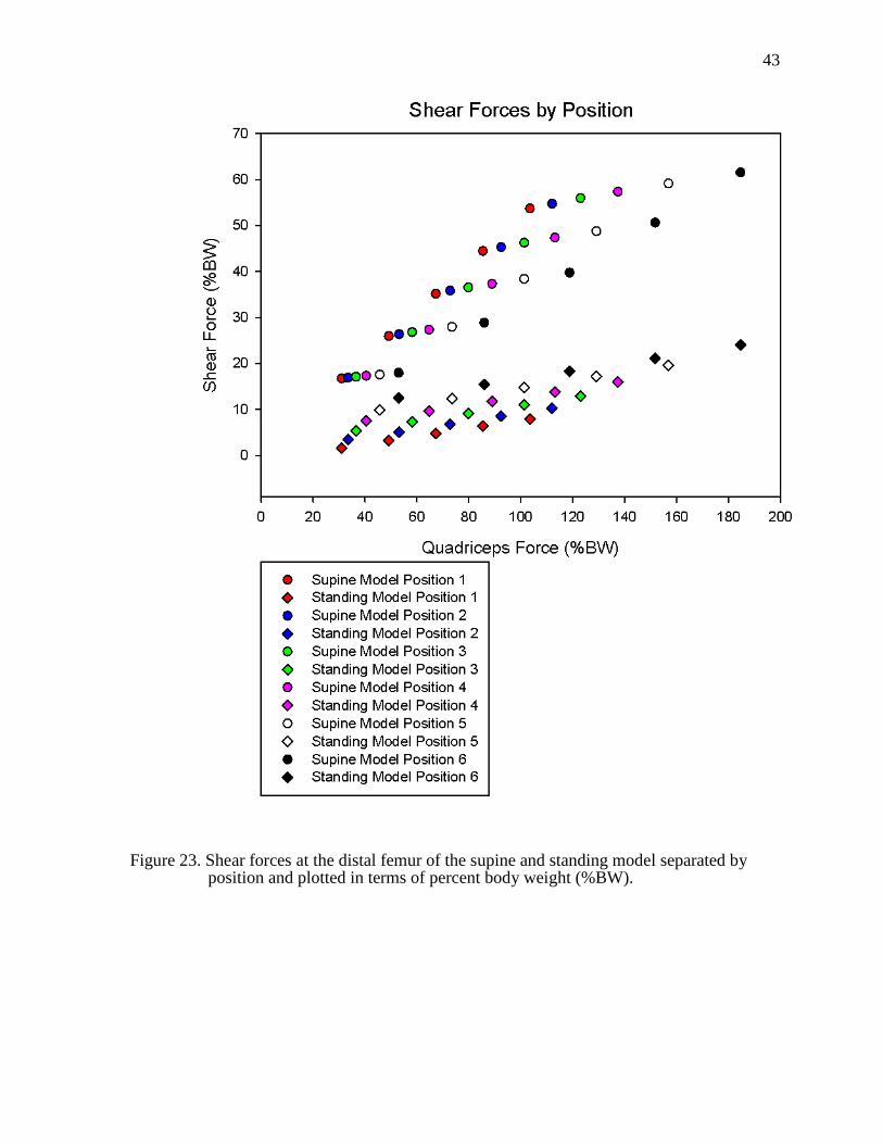
23. Shear forces at the distal femur of the supine and standing model separated by position and plotted in terms of percent body weight (%BW).. ...............................43

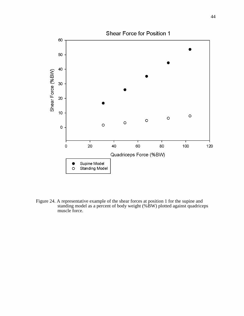
24. A representative example of the shear forces at position 1 for the supine and standing model as a percent of body weight (%BW) plotted against quadriceps muscle force............................................................................................44

1

1

CHAPTER 1 INTRODUCTION

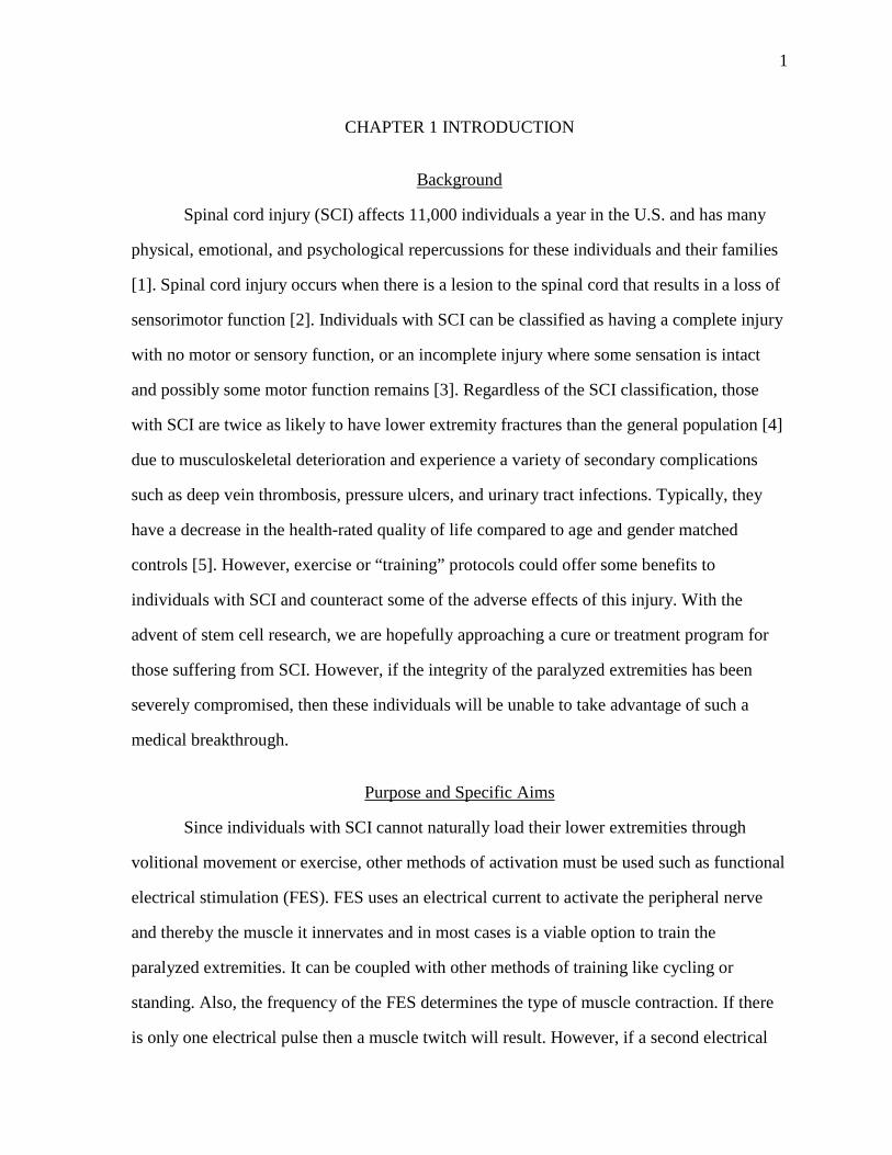
Background

Spinal cord injury (SCI) affects 11,000 individuals a year in the U.S. and has many

physical, emotional, and psychological repercussions for these individuals and their families

[1]. Spinal cord injury occurs when there is a lesion to the spinal cord that results in a loss of

sensorimotor function [2]. Individuals with SCI can be classified as having a complete injury

with no motor or sensory function, or an incomplete injury where some sensation is intact

and possibly some motor function remains [3]. Regardless of the SCI classification, those

with SCI are twice as likely to have lower extremity fractures than the general population [4]

due to musculoskeletal deterioration and experience a variety of secondary complications

such as deep vein thrombosis, pressure ulcers, and urinary tract infections. Typically, they

have a decrease in the health-rated quality of life compared to age and gender matched

controls [5]. However, exercise or “training” protocols could offer some benefits to

individuals with SCI and counteract some of the adverse effects of this injury. With the

advent of stem cell research, we are hopefully approaching a cure or treatment program for

those suffering from SCI. However, if the integrity of the paralyzed extremities has been

severely compromised, then these individuals will be unable to take advantage of such a

medical breakthrough.

Purpose and Specific Aims

Since individuals with SCI cannot naturally load their lower extremities through

volitional movement or exercise, other methods of activation must be used such as functional

electrical stimulation (FES). FES uses an electrical current to activate the peripheral nerve

and thereby the muscle it innervates and in most cases is a viable option to train the

paralyzed extremities. It can be coupled with other methods of training like cycling or

standing. Also, the frequency of the FES determines the type of muscle contraction. If there

is only one electrical pulse then a muscle twitch will result. However, if a second electrical

2

2

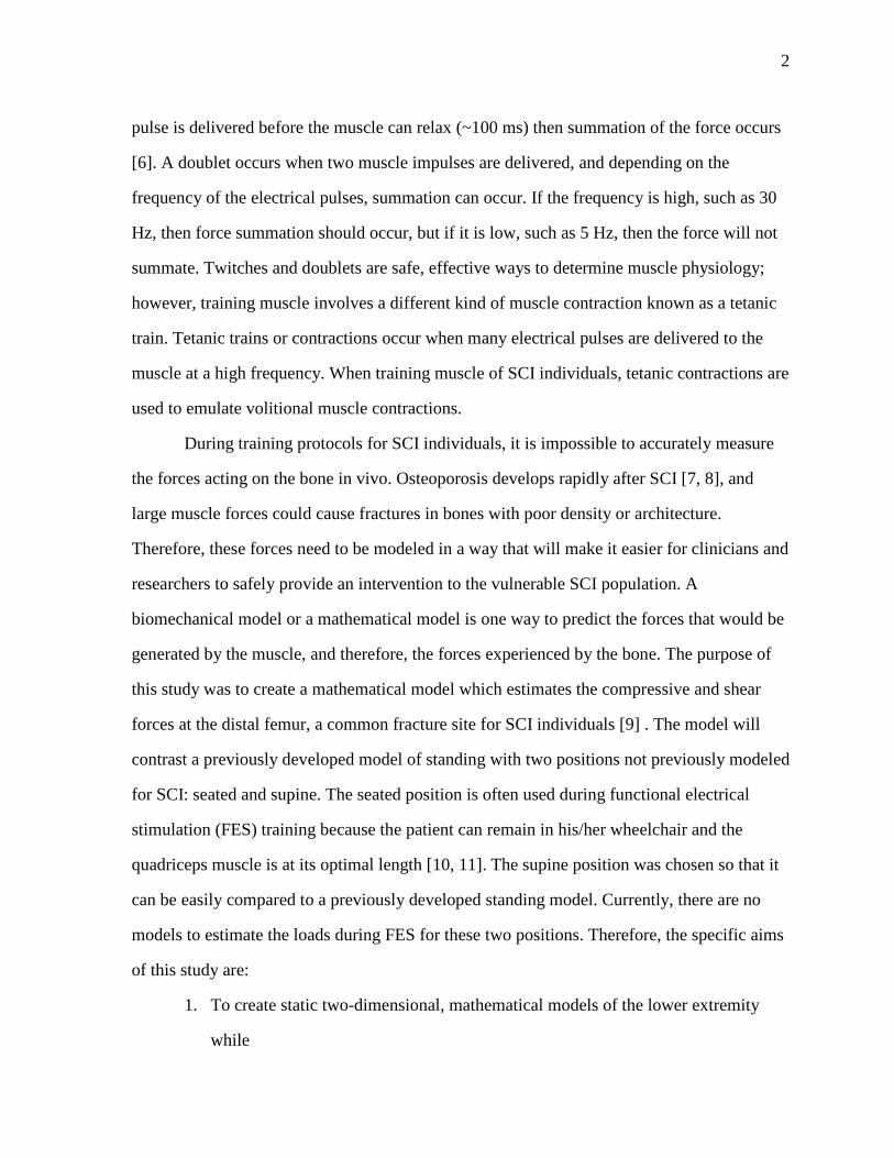
pulse is delivered before the muscle can relax (~100 ms) then summation of the force occurs

[6]. A doublet occurs when two muscle impulses are delivered, and depending on the

frequency of the electrical pulses, summation can occur. If the frequency is high, such as 30

Hz, then force summation should occur, but if it is low, such as 5 Hz, then the force will not

summate. Twitches and doublets are safe, effective ways to determine muscle physiology;

however, training muscle involves a different kind of muscle contraction known as a tetanic

train. Tetanic trains or contractions occur when many electrical pulses are delivered to the

muscle at a high frequency. When training muscle of SCI individuals, tetanic contractions are

used to emulate volitional muscle contractions.

During training protocols for SCI individuals, it is impossible to accurately measure

the forces acting on the bone in vivo. Osteoporosis develops rapidly after SCI [7, 8], and

large muscle forces could cause fractures in bones with poor density or architecture.

Therefore, these forces need to be modeled in a way that will make it easier for clinicians and

researchers to safely provide an intervention to the vulnerable SCI population. A

biomechanical model or a mathematical model is one way to predict the forces that would be

generated by the muscle, and therefore, the forces experienced by the bone. The purpose of

this study was to create a mathematical model which estimates the compressive and shear

forces at the distal femur, a common fracture site for SCI individuals [9] . The model will

contrast a previously developed model of standing with two positions not previously modeled

for SCI: seated and supine. The seated position is often used during functional electrical

stimulation (FES) training because the patient can remain in his/her wheelchair and the

quadriceps muscle is at its optimal length [10, 11]. The supine position was chosen so that it

can be easily compared to a previously developed standing model. Currently, there are no

models to estimate the loads during FES for these two positions. Therefore, the specific aims

of this study are:

1. To create static two-dimensional, mathematical models of the lower extremity

while

3

3

the subject is a) supine and b) seated.

2. To estimate the loading environment of the distal femur during functional

electrical stimulation training for those with SCI in the seated and supine

positions.

3. To compare shear and compressive forces generated at the distal femur in the

supine model to the standing model

4. To compare shear and compressive forces at the distal femur of the

seated model during a tetanic quadriceps muscle contraction and during a

doublet quadriceps muscle contraction.

5. To validate the supine model by comparing the predicted force at the tibial restraint

with the force measured during the experimental testing.

Hypothesis

The general hypothesis is that the standing model is superior to the alternative

positions (supine, seated) in terms of optimal compressive loads and minimizing dangerous

shear forces on the distal femur. The specific hypotheses are as follows:

Hypothesis 1: If the quadriceps force from the standing model and the supine model

remain the same and the angles of the lower limb are held constant, the

compressive forces will be significantly lower and the shear forces will be

significantly higher in the supine model.

Hypothesis 2: For the seated model, a doublet pulse will result in significantly lower

shear and compressive forces at the distal femur compared to a tetanic train.

4

4

CHAPTER 2 LITERATURE REVIEW

Muscle and Nerve Anatomy

The spinal cord is part of the central nervous system. It serves to transmit motor

commands from the brain to the periphery, and carries sensory information from the

periphery to the brain. The spinal cord originates at the brainstem, travels through the

foramen magnum in the base of the skull, and continues within the vertebral column

branching off and becoming peripheral nerves. These peripheral nerves are composed of

many axons; each axon branches further until it innervates a single muscle fiber.

Voluntary or volitional muscle contractions occur when an electrical signal travels

from the brain to the muscle via the spinal cord and its peripheral nerves. If these conduits for

electrical signals are damaged then the brain can no longer send commands to the muscle or

receive feedback from the muscle. A spinal cord injury is an example of such a disturbance

to the nervous system and can result in a loss of volitional movement. Typically, a SCI

causes an upper motor neuron lesion as well as a lower motor neuron legion. An upper motor

neuron lesion is a disruption of upper motor neuron pathways descending to muscles and

ascending sensory pathways from muscles, and a lower motor neuron lesion results in

damage to peripheral nerves at the level of the injury.

Musculoskeletal Adaptations Following SCI

Spinal cord injury (SCI) results in muscle atrophy [12] and a rapid decrease in bone

mineral density (BMD) of the paralyzed lower extremities due in part to the absence of

physiological loading [13]. Muscle contractions naturally load the skeletal system and

maintain BMD, but following a SCI this stimulus is removed. It has been observed that six

weeks after a SCI, lower extremity muscles experience a 45% decrease in cross-sectional

area compared to age-matched controls [14]. Also, there is a shift in fiber type to fast muscle

[15, 16]. Normally, human muscle contains a combination of fast and slow muscle but

following a SCI slow muscle transforms to fast muscle because it is more metabolically

5

5

efficient. Slow muscle, which is fatigue resistant, requires more oxygen, therefore, needs

more blood vessels and more surface area to accomodate them [11]. The muscle

transformation is reflected by an increase in myofibrillar adenosine

triphosphatase(mATPase) [17].

Spinal cord injury severely restricts gravitational and muscle stimuli on the paralyzed

extremities which are essential to maintaining bone density. When the bone is no longer

mechanically loaded the osteoclast activity outpaces the osteoblast activity resulting in a

decrease in bone mineral density and an alteration in bone microarchitecture. During the first

year following SCI, the BMD of cortical bone decrease 2% per month and trabecular bone

decreases 4% per month in the paralyzed extremities [18]. In a SCI femur, there is a 50% loss

of trabecular bone in the epiphyses and a 35% decrease in cortical wall thickness of the shaft

[8]. After a SCI, the trabecular lattice continues to be replaced with marrow [19] and a

steady-state BMD is reached between 3 and 8 years post-injury [8]. The steady state BMD of

SCI individuals is 50-60% less than those of non-SCI [20] which emphasizes the importance

in preventing such deterioration.

Methods and Implications of Training Individuals with SCI

Many methods have been developed attempting to prevent muscle atrophy and

osteoporosis in individuals with SCI including functional electrical stimulation (FES), FES

cycling, body weight supported treadmill training, and standing. The purpose of exercise is to

optimally stress muscle and bone in order to induce an advantageous adaptation and avoid

injury [21]. In general, muscle hypertrophy occurs if a muscle experiences a certain amount

of overload [20]. When a muscle experiences a large load through volitional activation or

elicited by electrical stimulation it will adapt and increase its force generating capabilities.

Bone has a similar response to training and to induce osteogenesis, bone formation, it needs

to experience a certain amount of mechanical load [22]. Osteocytes, bone cells, are very

sensitive to mechanical deformation or strain which results from fluid flow within the bone

6

6

and leads to bone adaptation [23]. According to Frost, bone modeling or formation occurs at

1500-3000 microstrain and bone remodeling or degradation occurs at 100-300 microstrain

[24]. Therefore, bone needs to have a certain amount of strain in order to prevent degradation

and osteoporosis. Following a SCI, it is crucial that muscle and bone are optimally loaded so

that they do not deteriorate. While there are many methods to train the paralyzed

musculoskeletal system of those with SCI; our lab has found that FES and FES coupled with

standing can radically alter musculoskeletal physiology, especially compared to other

training protocols.

Functional electrical stimulation (FES) uses a nerve to activate a muscle by an

electrical current. It has been effective in activating paralyzed muscles to attenuate BMD loss

[25, 26] and to prevent muscle atrophy after SCI [27]. FES can be used if there are no lower

motor neuron lesions which would prevent electrical activation of the target muscle.

Typically, if the muscle experiences adequate stimuli to induce muscle changes, then FES

results an increase in muscle cross sectional area [28, 29], an increase in oxidative capacity

[30, 31], and retention of slow muscle fiber [32]. For example, when stimulating wrist

extensors in tetraplegics, the group that received higher stimulation, and therefore, a higher

resistance force experienced an increase muscle strength compared to the low resistance

group [33]. Also, a quadriceps study showed a correlation between the magnitude of load and

the degree of muscle adaptation. The limb that received the higher load had a significant

increase in cross-sectional area, Type I fibers, and a capillary-to-fiber ratio compared to the

opposite limb [34]. Since muscle can retain its force generating capabilities through FES,

they can provide a substantial mechanical load and affect bone mineral density. In previous

work from our laboratory, unilateral FES of one soleus muscle resulted in a 31% increase in

BMD of the tibia compared to the tibia of the untrained limb the same individual [35, 36].

The BMD of the posterior region of the tibia also remained close to the BMD of non-SCI

individuals because the soleus stresses the tibia posteriorly [37]. It is essential to examine the

magnitude of bone loading required to induce bone remodeling.

7

7

Osteogenesis occurs when bone reaches a strain level of 1500-3000 microstrain [24].

However, with spinal cord injury individuals it can be difficult to safely deliver a significant

load to the lower extremities, because their atrophied muscles have reduced force generating

abilities and their osteoporotic bones are susceptible to fractures. Passive standing using a

standing frame or standing wheelchair is one way for individuals with SCI to mechanically

load their lower extremities. Generally, passive standing does not affect BMD [38, 39]

because the compressive load to the lower extremities is only 40% of body weight, as

estimated by the previous standing model [40]. The soleus study showed that a load of

approximately 150% of body weight was sufficient to cause an increase in BMD [35]. To

incorporate FES and standing, a standing exercise paradigm has recently been developed to

optimally load bone [40]. A 2-D model was created to examine the differences between

passive standing, active standing where the quadriceps are activated enough to support body

weight and active-resistive stance, where the quadriceps are activated enough to support

body weight and push against an external resistance. As hypothesized, active-resistance

stance produced the greatest amount of compressive force at the distal femur of 240% body

weight but shear force was less than 24% body weight [40]. Through this experimental

model the lower extremities can be optimally loaded while minimizing fracture-inducing

shear stress.

Rationale for Creating a Biomechanical Model

Although FES is an ideal stimulus to trigger adaptations in paralyzed muscle and

bone, those administering such interventions need to be aware of the potentially dangerous

repercussions. Those with spinal cord injury are twice as likely as the general population to

have a fracture [4] from routine activities. There is one published report of a bone fracture of

a SCI subject during FES. The authors attributed the lateral femoral condyle fracture to

maximal electrical stimulation while the knee was locked in 90° of flexion, muscle spasm

during the stimulation, severe osteoporosis, and an increase in muscle strength from regular

8

8

bouts of FES cycling [41]. Therefore, it is important to account for the change in bone

structure and to load the lower extremity in a safe way, in order to prevent such occurrences.

When administering FES training to a SCI cohort, it is crucial to understand the shear

and compressive forces that are generated. It is believed that the documented fracture during

FES was the result of a large shear force. In a biomechanical analysis of the knee, Smidt

demonstrated that a change in the knee angle corresponded to a change in the magnitude and

direction of the shear forces at the distal femur. The maximum posterior shear force (tibia

moving posteriorly on the femur) occurs when the knee is in 90° of flexion [42] , the same

knee angle of the reported fracture. Clinicians and researchers use FES with the knee flexed

to 90° because when a subject is seated and the knee is flexed at 90-100º the quadriceps

muscle is at its optimal length, therefore can generate its maximum torque [43]. The

quadriceps muscle can generate such a large torque because in this position the patella and

the femur have the greatest amount of contact [44-46]. Since the goal of FES is to prevent

muscle atrophy and attenuate bone loss, those training want to safely deliver the highest dose

possible to induce positive musculoskeletal adaptations.

One way to ensure safe training is to understand the forces that can be generated

during a specific loading environment and position. Since it is difficult to directly measure

the various forces on the bone in vivo, a model needs to be created to simulate the loading

conditions during FES. A two-dimensional, mathematical model can provide valuable insight

into the forces generated from certain loading conditions. Due to the simplicity of this model,

it is easy to use for clinicians and researchers and provides a cost effective alternative to

other models which require imaging. As stated earlier, a 2D, mathematical model has been

created to investigate the external forces, quadriceps muscle forces, and the shear and

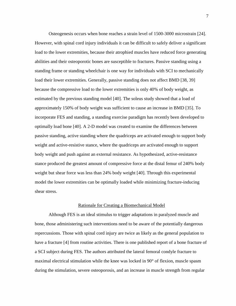
compressive forces at the distal femur during FES while standing [40]. Figure 1 shows the

free body diagram of the passive and active conditions used to determine the quadriceps

muscle force (Fig. 2) and subsequently the compressive and shear force at the distal femur

(Fig. 3). A range of resistive force, R, in terms of body weight were implemented in the

9

9

active condition model including 0%, 16.7%, 33.3%, 50%, and 67.7%. Figure 2 depicts the

quadriceps muscle force as the resistive force and the stance position change. Six standing

positions were used, resulting in different thigh and shank angles (Fig. 4). The greatest

quadriceps force, 190% of body weight, occurs at position 6, the most upright posture, with a

resistive force equivalent to 67.7% of body weight. While the largest compressive force is

also produced during that position and resistive force, 240% of body weight, shear force

remains relatively low at 24% of body weight. The standing model demonstrates that a large

compressive force could be applied to the distal femur during this standing exercise paradigm

while minimizing harmful shear forces.

One of the goals of this study is to develop a mathematical model for the supine

position to compare the compressive and shear forces at the distal femur to those generated in

the standing model. Another goal of the study is to create a seated mathematical model and

estimate the shear and compressive forces at the distal femur during two different loading

conditions. The first loading condition is a tetanic contraction which is elicited from the

quadriceps muscle; more specifically, the force that was previously reported to cause a

fracture (206 N) will be used. The second loading condition is the muscle contraction

resulting from a doublet pulse delivered to the quadriceps muscle [43]. The doublet protocol

was developed as a way to accurately measure muscle physiology without generating

dangerously high forces. However, the shear and compressive forces at the distal femur

during the doublet protocol have not been examined.

10

10

Figure 1. Schematic free body diagram of the lower body during (A) passive stance and (B) active (no added resistance, R = 0) and/or active–resistive stance (R = 16.7–67.7% BW). The internal forces from the quadriceps and patellar tendons (Fquad and Fpat, respectively) in (B) replace the Fpad in (A).

Source: Frey Law, L.A. and R.K. Shields, Femoral loads during passive, active, and active-resistive stance after spinal cord injury: a mathematical model. Clin Biomech (Bristol, Avon), 2004. 19(3): p. 313-21.

11

11

Figure 2. Modeled quadriceps forces are shown in percent body weight (% BW) during active and active–resistive stance with resistances ranging from 16.7% BW to 67.7% BW for each of the six stance postures.

Source: Frey Law, L.A. and R.K. Shields, Femoral loads during passive, active, and active-resistive stance after spinal cord injury: a mathematical model. Clin Biomech (Bristol, Avon), 2004. 19(3): p. 313-21.

12

12

Figure 3. Modeled distal femur compression (A) and shear (B) in terms of percent body weight are plotted for passive, active, and active–resistive stance at each of the six stance postures. Note the different scales between graph A and B.

Source: Frey Law, L.A. and R.K. Shields, Femoral loads during passive, active, and active-resistive stance after spinal cord injury: a mathematical model. Clin Biomech (Bristol, Avon), 2004. 19(3): p. 313-21.

13

13

Figure 4. Schematic representations of six possible stance postures for individuals with spinal cord injury (SCI) using an external frame (not shown).The arrow at the hip and the vertical line at the knee represent a hip support belt and a knee support pad, respectively. The feet are placed on the ground.

Source: Frey Law, L.A. and R.K. Shields, Femoral loads during passive, active, and active-resistive stance after spinal cord injury: a mathematical model. Clin Biomech (Bristol, Avon), 2004. 19(3): p. 313-21.

14

14

CHAPTER 3 METHODS

Mathematical Model

Supine Model

A two-dimensional, static, supine model has been developed to estimate the internal

forces at the distal femur during FES, and to compare these compressive and shear forces to

those in the standing model. The model assumes the human body is symmetric, and

therefore, only one lower extremity was modeled. This model consists of the thigh, shank,

and ankle represented as a three-bar linkage system (Fig. 5) which is consistent with the

standing model. The model is assumed to act as a rigid body since only small deflections will

occur when it is loaded by the quadriceps muscle group. The knee and ankle joints are

modeled as two-dimensional, frictionless, pin joints and the hip joint is a fixed support in the

x-direction, xhipF , and the y-direction, yhipF . Although the rectus femoris, one of the

quadriceps muscles, crosses the hip, the internal moment at the hip was assumed to be

negligible. The symbols, φ and α, are the angles from the vertical to the thigh and shank

segment, respectively. The standing model used a variety of thigh and shank angles to

examine six different positions of standing and Table 1 contains the values for φ and α. For

both models, anthropometric values are used to determine the masses, HATW thW , shW , and

ftW , lengths, thL , shL , and ftL , and center of masses, thCM and shCM of all of the segments

from a hypothetical subject with height = 1.73 m and weight = 68.04 kg (See Appendix A)

[47]. Although the mass of the thigh segment is fully supported, the distributed loaded was

modeled as a single vector acting on the thigh. A force transducer is contained in the tibial

restraint, AR , at a length, mL , from the knee joint which was arbitrarily chosen to be 0.400

meters. This force is perpendicular to the shank segment and, therefore its angle, β, changes

as the shank angle changes and can be defined as 90°-α.

When the quadriceps muscle is activated, it results in forces acting through the

quadriceps tendon, quadF , and patellar tendon, patF . While there is an internal moment at the

15

15

knee, it is due to the forces generated by the quadriceps, and therefore, is accounted for in the

governing force and moment equations. The quadriceps muscles are modeled as a single

vector as opposed to four vectors (one for each of the four quadriceps muscles). The supine

model assumes that the horizontal components of quadF and patF are equal and opposite [48,

49] because the vertical components of these forces in standing model were assumed to be

equivalent. Also, since the internal angle of the quadriceps tendon and the patellar tendon is

less than 10° [50], it can be assumed that the tendon forces act at a 5° angle from the thigh

and shank segments, respectively (Fig. 6). The relationship between then quadriceps tendon

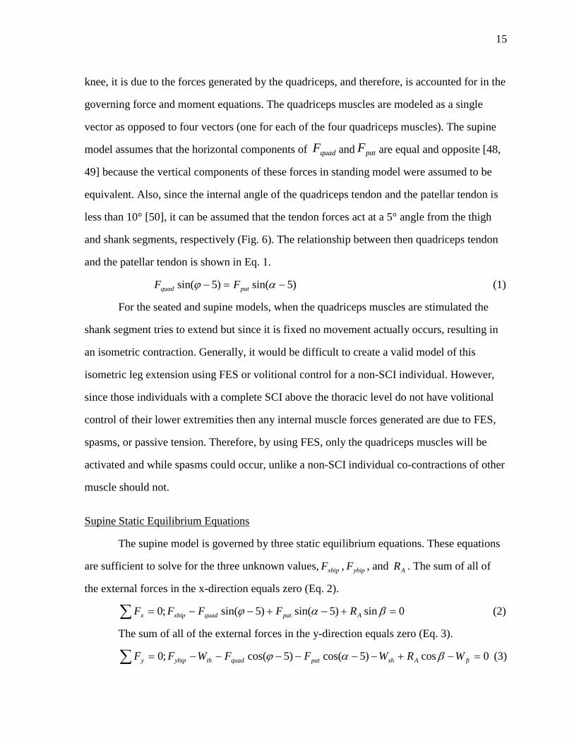
and the patellar tendon is shown in Eq. 1.

)5sin()5sin( −=− αϕ patquad FF (1)

For the seated and supine models, when the quadriceps muscles are stimulated the

shank segment tries to extend but since it is fixed no movement actually occurs, resulting in

an isometric contraction. Generally, it would be difficult to create a valid model of this

isometric leg extension using FES or volitional control for a non-SCI individual. However,

since those individuals with a complete SCI above the thoracic level do not have volitional

control of their lower extremities then any internal muscle forces generated are due to FES,

spasms, or passive tension. Therefore, by using FES, only the quadriceps muscles will be

activated and while spasms could occur, unlike a non-SCI individual co-contractions of other

muscle should not.

Supine Static Equilibrium Equations

The supine model is governed by three static equilibrium equations. These equations

are sufficient to solve for the three unknown values, xhipF , yhipF , and AR . The sum of all of

the external forces in the x-direction equals zero (Eq. 2).

0sin)5sin()5sin(;0 =+−+−−=∑ βαϕ Apatquadxhipx RFFFF (2)

The sum of all of the external forces in the y-direction equals zero (Eq. 3).

0cos)5cos()5cos(;0 =−+−−−−−−=∑ ftAshpatquadthyhipy WRWFFWFF βαϕ (3)

16

16

The sum of all external moments equals zero (Eq. 4).

(4)

These equations for were solved for xhipF , yhipF , and AR using Matlab computer

software (Prentiss Hall, New Jersey, USA) and the computer code is located in Appendix B.

The external forces, segment mass and muscles forces were known along with moment arms,

segment length and center of mass of the segments. Since the location of the force

transducers changes between the standing model and the supine model, it was necessary to

have the degree of muscle activation remain uniform. In order to accurately compare these

models, the quadriceps force and thereby the patellar force (Eq. 1) from the standing model

were used in the supine model.

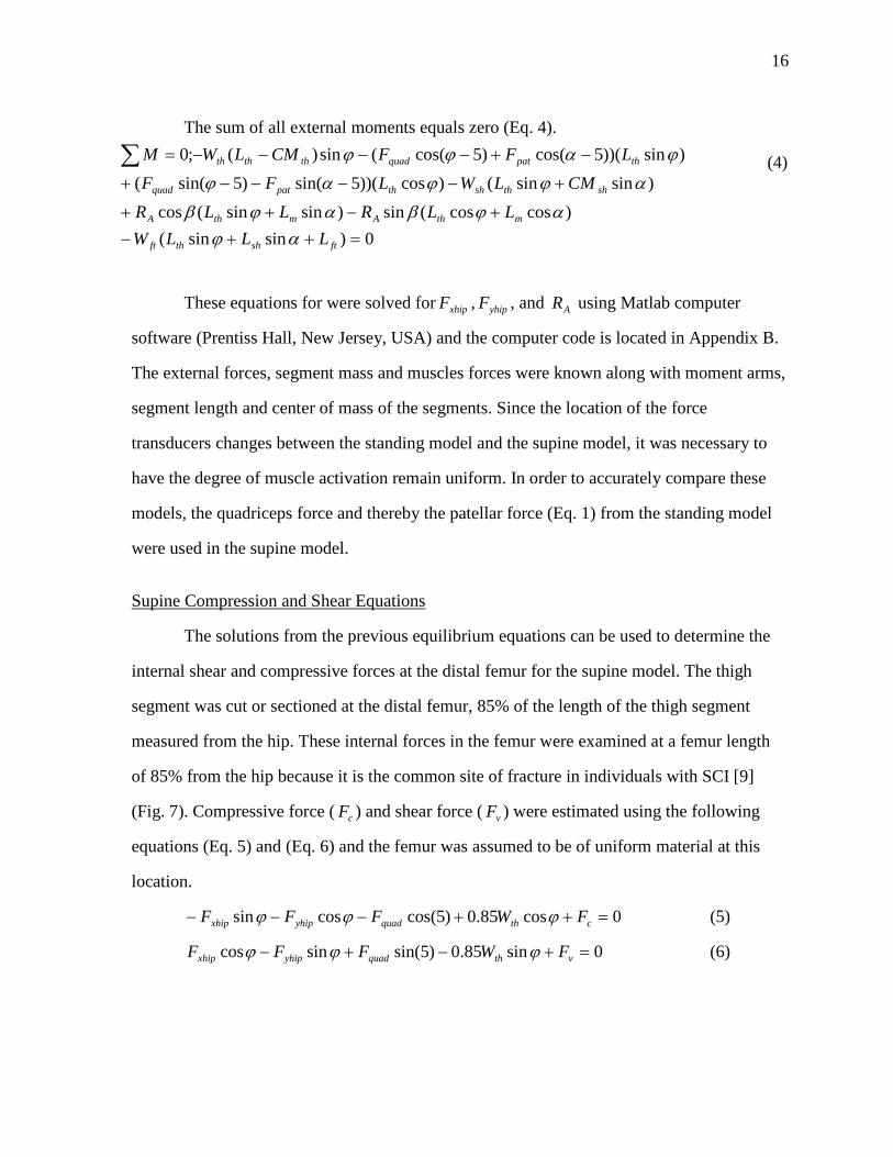
Supine Compression and Shear Equations

The solutions from the previous equilibrium equations can be used to determine the

internal shear and compressive forces at the distal femur for the supine model. The thigh

segment was cut or sectioned at the distal femur, 85% of the length of the thigh segment

measured from the hip. These internal forces in the femur were examined at a femur length

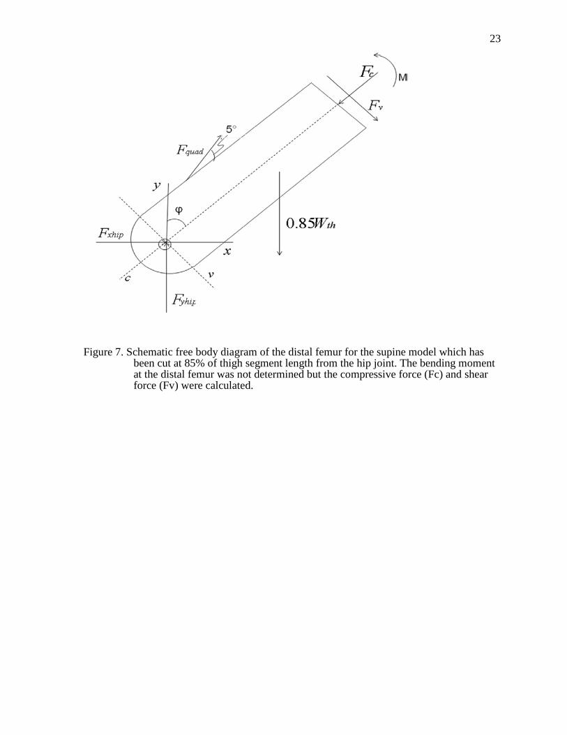
of 85% from the hip because it is the common site of fracture in individuals with SCI [9]

(Fig. 7). Compressive force ( cF ) and shear force ( vF ) were estimated using the following

equations (Eq. 5) and (Eq. 6) and the femur was assumed to be of uniform material at this

location.

0cos85.0)5cos(cossin =++−−− cthquadyhipxhip FWFFF ϕϕϕ (5)

0sin85.0)5sin(sincos =+−+− vthquadyhipxhip FWFFF ϕϕϕ (6)

0)sinsin()coscos(sin)sinsin(cos

)sinsin()cos))(5sin()5sin((

)sin))(5cos()5cos((sin)(;0

=++−+−++

+−−−−+

−+−−−−=∑

ftshthft

mthAmthA

shthshthpatquad

thpatquadththth

LLLWLLRLLR

CMLWLFFLFFCMLWM

αϕαϕβαϕβ

αϕϕαϕ

ϕαϕϕ

17

17

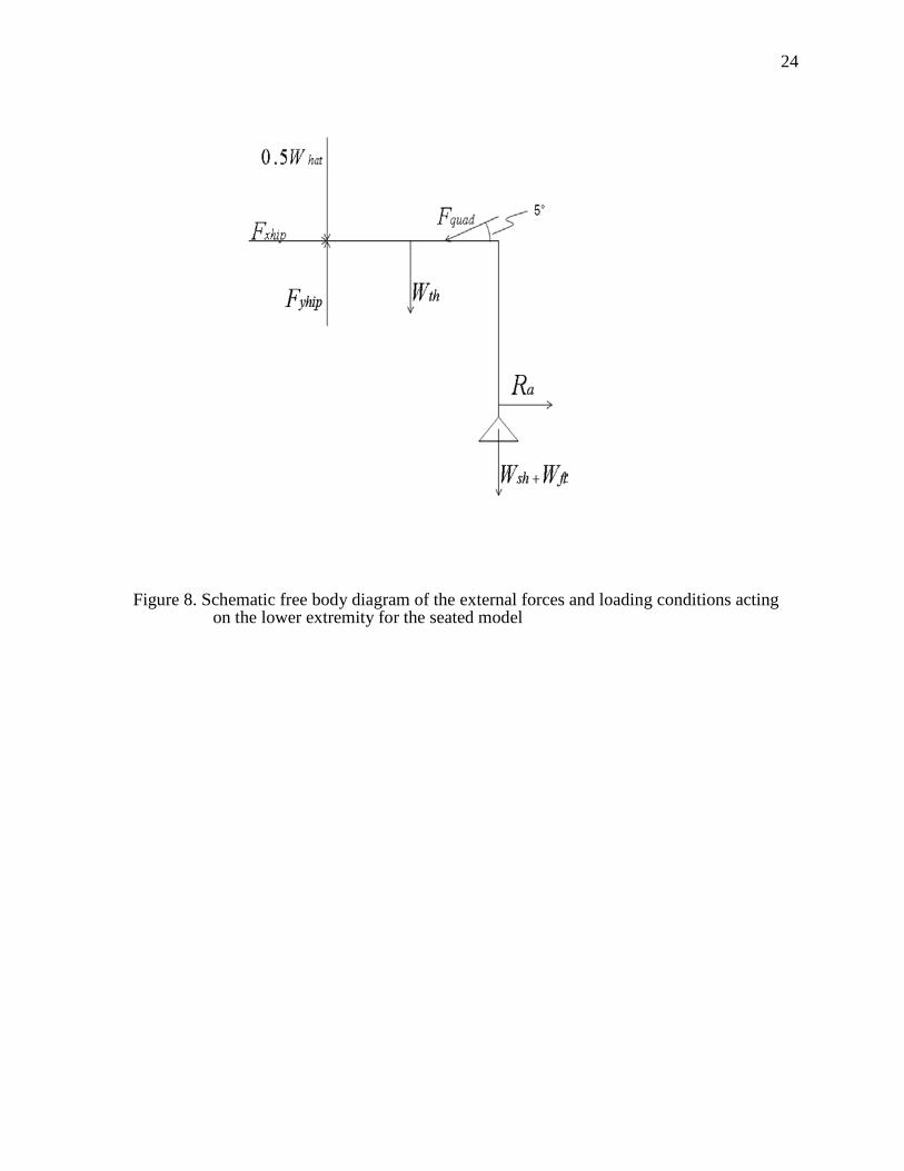
Seated Model

In order to evaluate the second hypothesis, a two-dimensional, static, seated model

was developed. Similar to the supine model, a three-bar linkage system was used for the

lower extremity, the knee and ankle joints were modeled as frictionless, pin joints, and the

hip joint was a fixed support. The seated model (Fig. 8) also measures force at the distal tibia

( AR ) like the supine model but it and the distance from the knee joint (lateral femoral

condyle) to the transducer ( mL ) are determined experimentally. The force at the tibial

restraint is assumed to be normal or perpendicular to the shank segment. Also, the knee angle

or the angle between the thigh and shank segments is 90°. The quadriceps muscle, quadF , is

directed towards the hip and is 5° from the thigh segment, like the supine model.

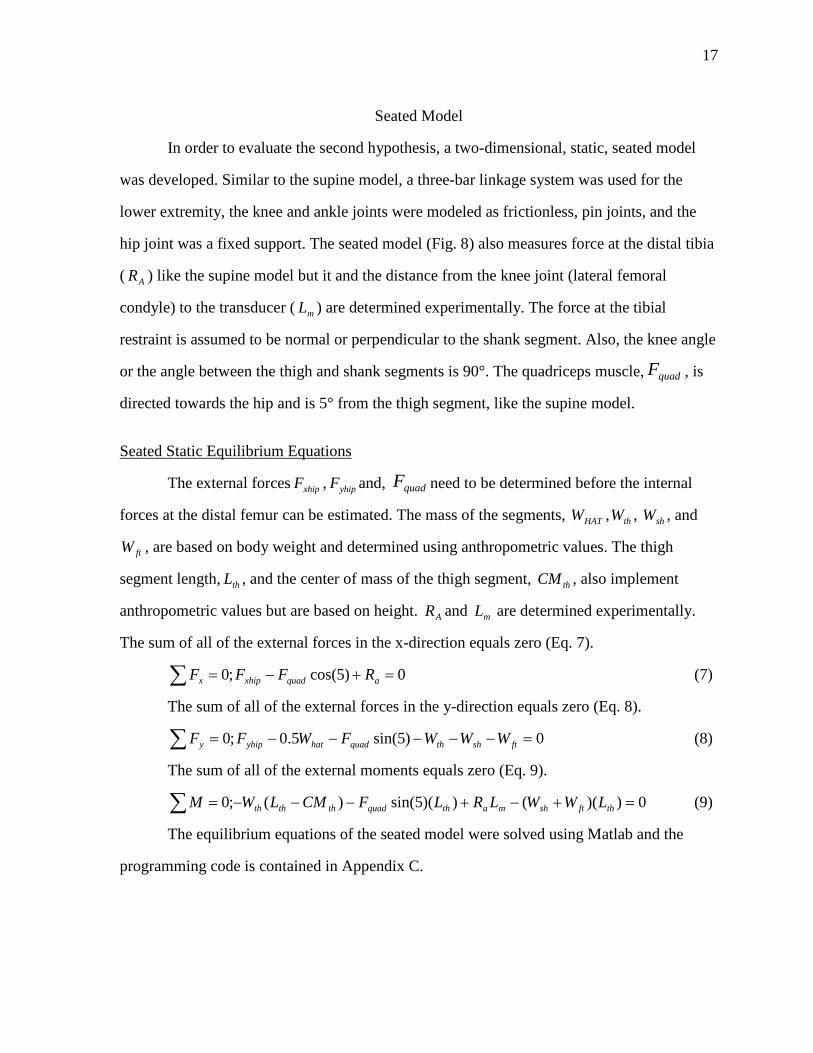
Seated Static Equilibrium Equations

The external forces xhipF , yhipF and, quadF need to be determined before the internal

forces at the distal femur can be estimated. The mass of the segments, HATW , thW , shW , and

ftW , are based on body weight and determined using anthropometric values. The thigh

segment length, thL , and the center of mass of the thigh segment, thCM , also implement

anthropometric values but are based on height. AR and mL are determined experimentally.

The sum of all of the external forces in the x-direction equals zero (Eq. 7).

0)5cos(;0 =+−=∑ aquadxhipx RFFF (7)

The sum of all of the external forces in the y-direction equals zero (Eq. 8).

0)5sin(5.0;0 =−−−−−=∑ ftshthquadhatyhipy WWWFWFF (8)

The sum of all of the external moments equals zero (Eq. 9).

0))(())(5sin()(;0 =+−+−−−=∑ thftshmathquadththth LWWLRLFCMLWM (9)

The equilibrium equations of the seated model were solved using Matlab and the

programming code is contained in Appendix C.

18

18

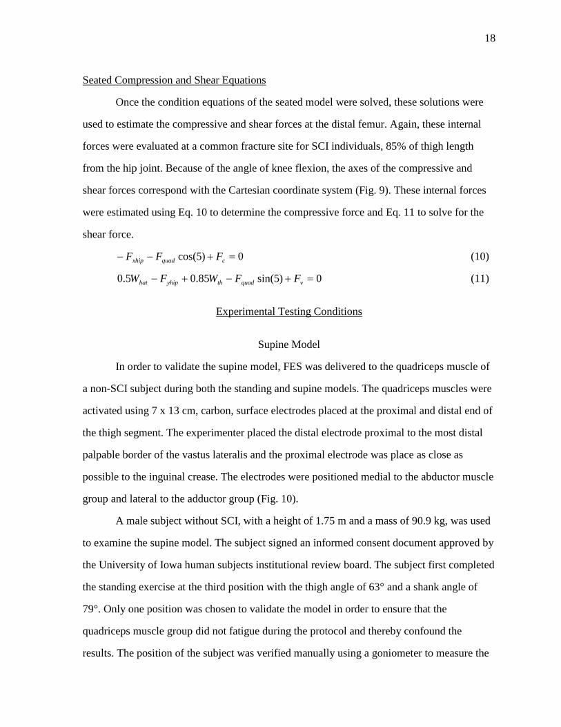
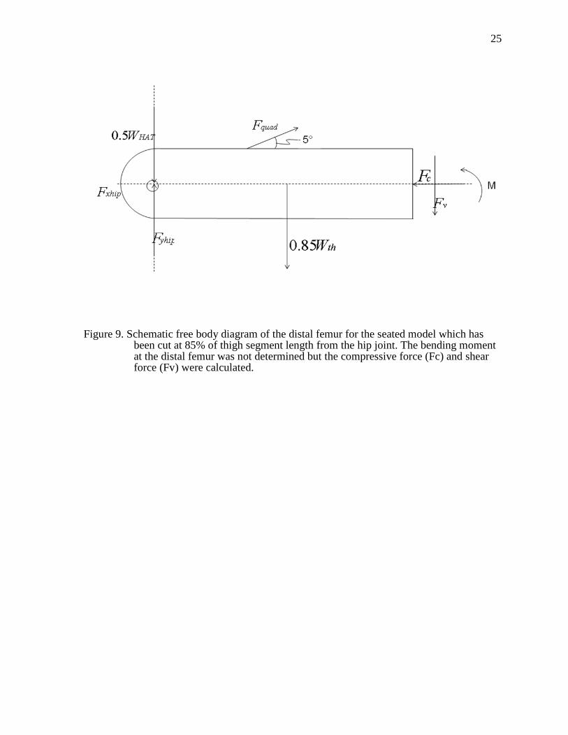
Seated Compression and Shear Equations

Once the condition equations of the seated model were solved, these solutions were

used to estimate the compressive and shear forces at the distal femur. Again, these internal

forces were evaluated at a common fracture site for SCI individuals, 85% of thigh length

from the hip joint. Because of the angle of knee flexion, the axes of the compressive and

shear forces correspond with the Cartesian coordinate system (Fig. 9). These internal forces

were estimated using Eq. 10 to determine the compressive force and Eq. 11 to solve for the

shear force.

0)5cos( =+−− cquadxhip FFF (10)

0)5sin(85.05.0 =+−+− vquadthyhiphat FFWFW (11)

Experimental Testing Conditions

Supine Model

In order to validate the supine model, FES was delivered to the quadriceps muscle of

a non-SCI subject during both the standing and supine models. The quadriceps muscles were

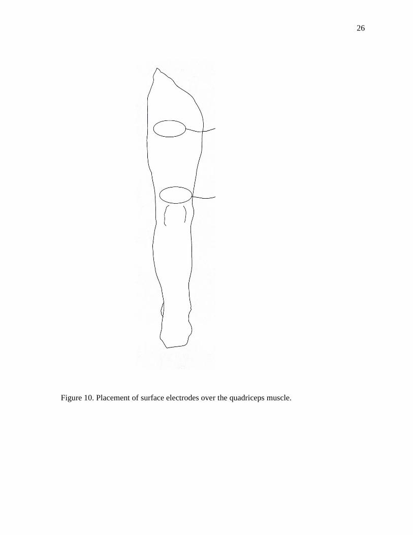
activated using 7 x 13 cm, carbon, surface electrodes placed at the proximal and distal end of

the thigh segment. The experimenter placed the distal electrode proximal to the most distal

palpable border of the vastus lateralis and the proximal electrode was place as close as

possible to the inguinal crease. The electrodes were positioned medial to the abductor muscle

group and lateral to the adductor group (Fig. 10).

A male subject without SCI, with a height of 1.75 m and a mass of 90.9 kg, was used

to examine the supine model. The subject signed an informed consent document approved by

the University of Iowa human subjects institutional review board. The subject first completed

the standing exercise at the third position with the thigh angle of 63° and a shank angle of

79°. Only one position was chosen to validate the model in order to ensure that the

quadriceps muscle group did not fatigue during the protocol and thereby confound the

results. The position of the subject was verified manually using a goniometer to measure the

19

19

angle of the knee. A current of 90 mA was chosen because it produced a sufficient force

reading and was well tolerated by the subject without spinal cord injury. Also, the supine

model predicted high shear forces during high quadriceps muscle force; therefore, a low

current of 90 mA was used to activate the muscle in case these predictions were accurate.

Five trains were delivered to the quadriceps muscle using an Infinity Plus Clinical Portable

Electrotherapy system (Empi, St. Paul, MN). The trains had a frequency of 20 Hz for a

duration of 5 seconds followed by 5 seconds of rest. The stimulus pulse width was 200

microseconds. The force generated by the quadriceps muscle was measured by a force

transducer at the knee (Interface 1500 ASK-200, Scottsdale, AZ). Using the peak force of the

five trains and the mathematical standing model, the quadriceps muscle force was obtained.

The subject was then asked to lay supine with the same lower extremity position as

the standing model to examine the supine model (Fig. 11). The electrodes remained in the

same position as the standing protocol and therefore the same amount of current should yield

the same quadriceps muscle force. A belt was safely fastened across the subject’s abdomen to

secure his trunk. The leg was attached to the mechanical arm of the isokinetic dynamometer

(KinCom) using a padded strap that passed behind the posterior surface of the shank and

pulled it into contact with the transducer. The transducer was contained in the mechanical

arm of the KinCom and cups the anterior surface of the shank. The adjustability of the

mechanical arm and the height of the seat allowed at the hip and the knee positions to be

easily changed. The third position, with respect to thigh angle and shank angle, from the

standing model was simulated in the supine position. Once the subject was secured to the

KinCom, a goniometer was used to manually verify the segment angles and any adjustments

to position were made.

The quadriceps muscle was activated using the same stimulator as the standing model

with the same 90 mA current. The stimulator delivered five 20 Hz trains for 5 seconds

followed by 5 seconds of rest. The force at the tibial restraint, AR , was recorded and

compared to the force obtained from the mathematical supine model.

20

20

Seated Model

Experimental measurements need to be collected as parameter inputs for the

mathematical seated model. One SCI male was asked to participate in the doublet stimulation

protocol [43]. The subject remained in his wheelchair throughout the collection (Fig.12). The

subject signed an informed consent document approved by the University of Iowa human

subjects institutional review board. The anterior surface of the ankle was in contact with the

force transducer (1500ASK-200, Interface, Scottsdale, AZ). The distance from the force

transducer to the lateral femoral condyle was measured and recorded as the moment arm. The

subject was positioned so that the knee was in 90° of flexion which was verified manually

using a goniometer. Surface electrodes were positioned over the quadriceps muscle using the

same placement method as the supine model. The previous publication [43] concluded that

the peak force elicited by a doublet occurred at a frequency of 30 Hz. While the entire

doublet force-frequency curve was completed to gain insights into the muscle physiology of

the subject’s quadriceps muscle, only the 30 Hz condition was used for this project. At 30

Hz, three doublets were delivered to the quadriceps muscle, separated by 2 seconds of rest.

Data Collection and Analysis

For all three experimental protocols, the analog force signal was amplified and

converted to a digital signal using 12-bit resolution analog-to-digital converter with a

sampling rate of 2,000 samples per second. Datapac 2K2 software (RUN Technologies,

Mission Viejo, CA) was used to analyze the digital force signals. The five peak forces (the

maximum amplitude of the force signal) for the standing and the supine models were

determined and averaged. The peak forces from the three doublet twitches were also were

averaged and recorded.

21

21

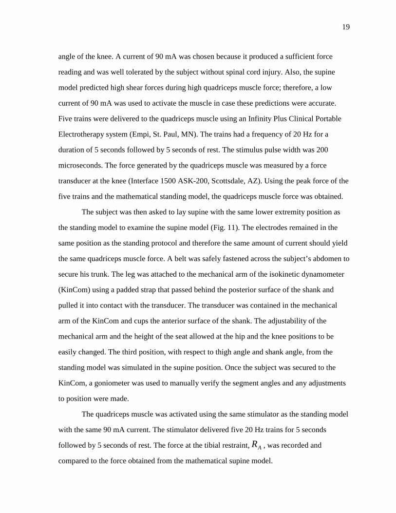
Position 1 2 3 4 5 6

φ 55° 59° 63° 67° 71° 75°

α 75° 77° 79° 81° 83° 85°

Table 1. The six supine positions with the corresponding thigh angle (φ) and shank angle (α).

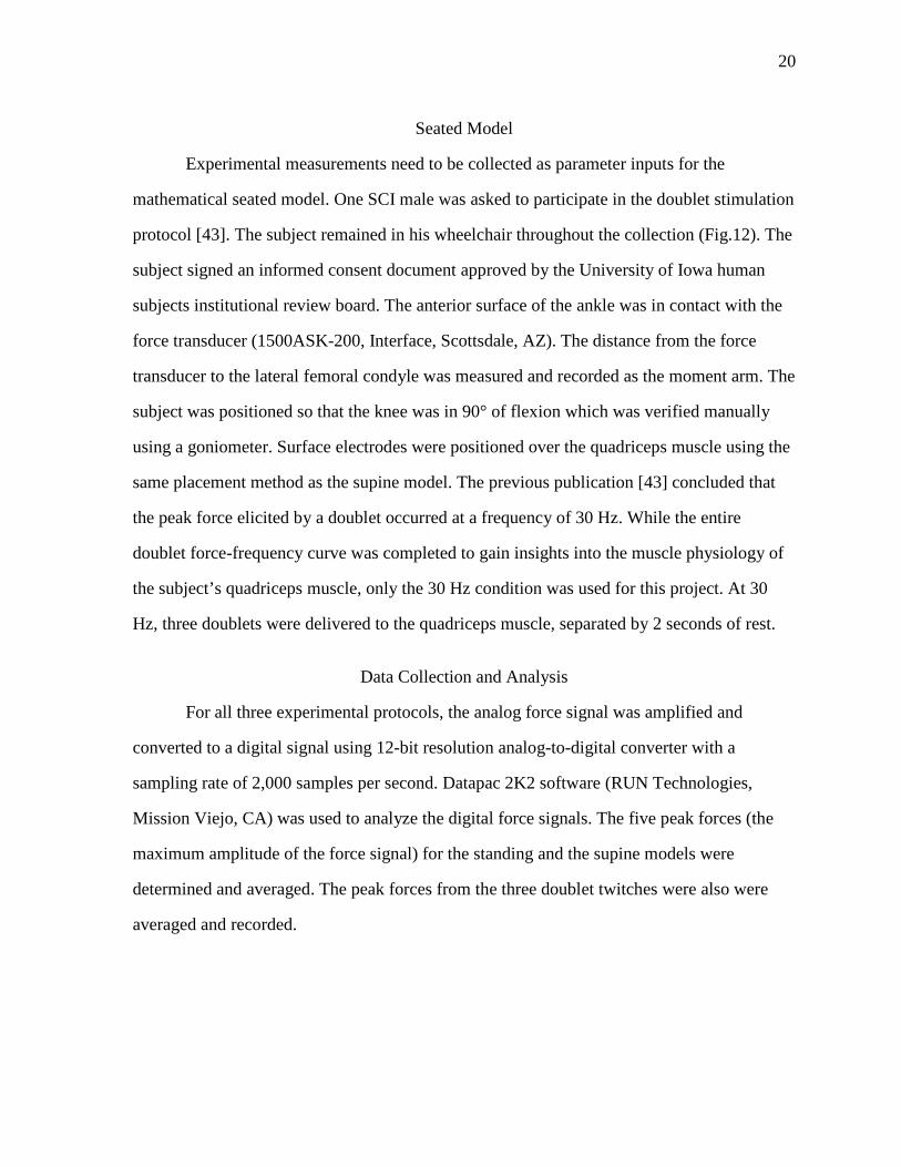
Figure 5. Schematic free body diagram of the external forces and loading conditions acting on the lower extremity for the supine model.

22

22

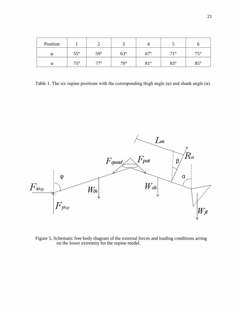
Figure 6. Schematic representation of the relationship between the quadriceps tendon or muscle (Fquad) and the patellar tendon (Fpat) at the knee joint.

23

23

Figure 7. Schematic free body diagram of the distal femur for the supine model which has been cut at 85% of thigh segment length from the hip joint. The bending moment at the distal femur was not determined but the compressive force (Fc) and shear force (Fv) were calculated.

24

24

Figure 8. Schematic free body diagram of the external forces and loading conditions acting on the lower extremity for the seated model

25

25

Figure 9. Schematic free body diagram of the distal femur for the seated model which has been cut at 85% of thigh segment length from the hip joint. The bending moment at the distal femur was not determined but the compressive force (Fc) and shear force (Fv) were calculated.

26

26

Figure 10. Placement of surface electrodes over the quadriceps muscle.

27

27

Figure 11. Non-SCI male positioned on the KinCom for the experimental supine model.

28

28

Figure 12. Schematic of the experimental seated model of the doublet stimulation protocol.

29

29

CHAPTER 4 RESULTS

Experimental Results

The mathematical model for the seated position required the tibial restraint force and

the moment arm to be determined experimentally. A SCI individual was positioned in his

wheelchair with his knee in 90° of flexion. The distance from the lateral femoral condyles to

the force transducer at the distal tibia was measured and recorded as 0.321 m. The peak force

for the doublet quadriceps muscle contraction occurred at 30 Hz and was equivalent to 13.3

kg. The subject’s height and weight are 1.93 m and 70.45 kg, respectively. The peak force

and moment arm for the tetanic quadriceps muscle contraction are 20.8 kg and 0.451 m,

respectively, and these were taken from the Hartkopp study which resulted bone fracture

[41]. Since the height and weight of the subject were not cited in the manuscript, the

hypothetical subject weight of 68.04 kg and height of 1.73 m were used.

Mathematical Model Predictions

Supine Model Predictions

The model condition equations were used to solve for the three unknowns of the

system, AR , xhipF , yhipF . The force at the tibial restraint and the horizontal and vertical

forces at the hip are plotted in Figs. 13, 14, and 15, respectively, at six supine positions with

five different quadriceps muscle forces at each position. The tibial restraint force increases as

quadriceps muscle force increases and ranges from 21.2% to 61.7% of body weight. Position

1 has the highest tibial restraint forces for each of the five groups of quadriceps force

compared to the other positions with position 6 having the lowest forces. However, the

horizontal force at the hip is inversely related to the quadriceps force and has a range of -

1.84% to -16.0% of body weight. For the horizontal force, position 1 has the largest

magnitude of force compared to the other positions in each of the five groups of forces with

position 6 having the lowest magnitude. The vertical force at the hip ranges from 21.2% to

30

30

54.1% and is directly related to the quadriceps force. Position 6 and position 1 have the

highest and lowest vertical forces, respectively, compared to the other positions in each of the

five clusters.

The values determined by the equilibrium equations were used to calculate the

compressive and shear forces at the distal femur which are plotted in Figs. 16 and 17,

respectively. The compressive force is positively correlated to quadriceps force. It ranges

from 33.1% of body weight at position 1 to 191.1% of body weight at position 6. Shear force

increases as the quadriceps force increases and ranges from 16.7% to 61.5% of body weight.

At position 6, the distal femur experiences the highest amount of shear force compared to the

other positions and position 1 has the lowest shear force. In position 6, the leg is almost fully

extended and therefore has the longest moment arm.

Figure 18 shows all of five variables; tibial restraint force, the horizontal and vertical

forces at the hip, and the compressive and shear forces at the distal femur at position 1. The

tibial restraint force, vertical force at the hip, and shear force at the distal femur have a

similar relationship and all show a slight increase as the amount of quadriceps force

increases. The horizontal force at the hip is much lower than the other forces and has indirect

relationship with the quadriceps force. The compressive force at the distal femur has the

largest magnitude of all the variables and has the greatest amount of increase with respect to

quadriceps force. Since all of the positions have similar trends and inter-variable

relationships, position 1 is shown as a representative example.

Supine and Standing Model Comparisons

In order to examine the internal forces at the distal femur, the compressive and shear

forces for both supine and standing mathematical models were plotted. It was predicted that

the standing model would estimate higher compressive force and lower shear forces at the

distal femur compared to the supine model. The compressive forces of the supine model and

the standing models are plotted against quadriceps force in Fig. 19. The standing model

31

31

predicts much higher compressive force compared to the supine model. The compressive

force of the standing model ranges from 75% to 240% of body weight. In order to discern

which values in the supine model correspond to the standing model, the compressive force is

also graphed by position in Fig. 20 but Fig. 21 is a representative example of compressive

force at the first position which is much clearer than Fig 20. Fig. 21 shows the compressive

forces of the supine and standing model at the distal femur. At each position, the standing

model had higher compressive force than the supine model which was expected because the

supine model excludes the weight of the trunk, head, and upper body.

Shear force was also examined in Figs. 22-24 similarly to compressive force. Figure

22 shows that the supine model estimated more shear force at the distal femur compared to

the standing model. While it is easy to see that the supine model tended to have more shear

force, it is difficult to match the quadriceps force corresponding to each model so Fig. 23

plotted the models by position. The graphs are separated further to only show one position,

Fig. 24, which plots the shear force of both models at the first position. Since all of the

positions follow a similar pattern only position 1 is included. At each particular quadriceps

force, the supine model estimates more shear in the distal femur than the standing model.

This is true because in the supine model the force opposing the quadriceps muscle is acting at

the distal tibia, the tibial restraint, and in the standing model this force is at the knee. In the

supine model, the point of resistance is more distal than the standing model and this

increased distance from the force transducer to the hip corresponds to an increase in shear

force.

Seated Model Predictions

A seated model was developed to determine how the forces at the distal femur differ

between a tetanic contraction and a doublet pulse to the quadriceps muscle. It was

hypothesized that at 90° of knee flexion, tetanic activation of the quadriceps muscle would

result in higher compressive and shear forces at the distal femur. The three independent,

32

32

equilibrium equations from the seated model and then compressive and shear equations were

solved to determine the five unknowns of the system. The quadriceps muscle force, the

horizontal and vertical forces at the hip, and, the compressive and shear forces at the distal

femur for both types of stimuli are shown in Table 2. All of the forces are much higher for

the tetanic muscle contractions compared to the doublet contractions with a compressive

force of 477% of body weight and a shear force of 68.6% body weight. However, the

compressive and shear forces that resulted from a doublet pulse were 38.3% and 29.3% body

weight, respectively. These results support the second hypothesis and are not surprising

because the doublet pulse results in a much lower quadriceps force than the tetanic

contraction.

Validity of Mathematical Models

In order to determine the accuracy a mathematical model, it needs to be validated

through experimental testing. Because the supine and the seated model are estimating the

compressive and shear forces at the distal femur, validation cannot be performed non-

invasively. However, validation of the force at the tibial restraint for the supine model could

be tested. The predicted force at the tibial restraint determined by the quadriceps force from

the standing model was 26.6 kg or 29.3% of body weight. The force measured at the tibial

restraint during the experimental supine position was 25.7 kg or 28.3% of body weight. The

percent error calculated between the predicted value and the experimental value was 3.4%.

33

33

Figure 13. The supine model predictions for the forces at the tibial restraint, AR , at various quadriceps muscle forces for the six different supine positions are graphed in terms of percent body weight (%BW).

34

34 Figure 14. The estimates of the horizontal forces at the hip, xhipF, for the supine model at

various quadriceps muscle forces for the six different supine positions are plotted in terms of percent body weight (%BW).

35

35 Figure 15. The supine model estimates of the vertical forces at the hip, yhipF, are plotted in

terms of percent body weight (%BW) for the six supine position with five different quadriceps muscle forces at each position.

36

36

Figure 16. The compressive forces, cF , estimated at the distal femur for the supine model in percent body weight (%BW) and graphed against quadriceps force.

37

37

Figure 17. The shear forces, vF , estimated at the distal femur for the supine model in percent body weight (%BW) and graphed against quadriceps force.

38

38

Figure 18. The estimates from the supine model for the tibial restraint force, the horizontal and vertical forces at the hip, and the compressive and shear forces at the distal femur for position 1 at five quadriceps forces.

39

39

Figure 19. The compressive forces at the distal femur for the supine model and the standing model are plotted in terms of body weight (%BW) with respect to quadriceps muscle force.

40

40

Figure 20. Compressive forces at the distal femur of the supine and standing models separated by position and plotted in terms of percent body weight (%BW)

41

41

Figure 21. A representative example of the compressive forces at the distal femur of position 1 for the supine and standing models as a percent of body weight (%BW) plotted against quadriceps muscle force.

42

42

Figure 22. The shear forces at the distal femur for both models, supine and standing, are plotted in terms of percent body weight (%BW) as a function of quadriceps muscle force.

43

43

Figure 23. Shear forces at the distal femur of the supine and standing model separated by position and plotted in terms of percent body weight (%BW).

44

44

Figure 24. A representative example of the shear forces at position 1 for the supine and standing model as a percent of body weight (%BW) plotted against quadriceps muscle force.

45

45

Stimulus Condition Fquad (%BW) Fxhip (%BW) Fyhip (%BW) Fc (%BW) Fv (%BW)

Tetanic 255 223 71.9 477 52.0

Doublet 28.7 9.72 52.1 38.3 12.5

Table 2. The solution to the five unknowns of the seated model for tetanic and doublet pulses are quadriceps force (Fquad), the horizontal force at the hip (Fxhip), the vertical force at the hip (Fyhip), compressive force at the distal femur (Fc), and shear force at the distal femur (Fv) and are reported in terms of percent body weight.

46

46

CHAPTER 5 DISCUSSION

The purposes of this study were: 1) to create two-dimensional, static models of the

lower extremity in the supine position and the seated position, 2) to estimate the compressive

and shear forces at the distal femur for both positions during FES, 3) to compare the internal

compressive and shear forces generated at the distal femur from the standing model with

those in the supine model, 4) to compare the compressive and shear forces at the distal femur

of the seated model during tetanic and doublet quadriceps muscle contraction, and 5) to

validate the supine model. Schematic free body diagrams were created to model the lower

extremity for the supine and seated positions. Three, independent equilibrium equations were

created for each of the two-dimensional, static models and two additional equations were

obtained from the cut distal femur. By solving this system of equations, the compressive and

shear forces at the distal femur for each of the conditions were determined. The primary

findings of the study which supported both of the hypotheses are 1) the standing model

estimated more compressive force and less shear force compared to the supine model, and 2)

the tetanic quadriceps muscle contraction in the seated model resulted in higher estimated

compressive and shear forces compared to the doublet quadriceps muscle contraction. Also,

the validation testing revealed that only 3.4% error occurred between the force predicted by

the supine model and the force measure for the tibial restraint. This low percent error could

be interpreted as the supine model at least accurately predicting the external force at the tibial

restraint.

There is much debate in the field of exercise science surrounding the most effective

method of mechanically loading bone: muscle or gravity [51-54] . Frost’s mechanostat theory

supports that the greatest mechanical loading of bone is predominately due to muscle forces

[22, 55]. However, after periods of extended bed rest [56] or space flight [57, 58] there is a

significant decrease in BMD due to a loss of gravitational load. It is difficult and unnecessary

to separate these mechanical loading mechanisms because a combination of both should yield

47

47

greatest preservation of BMD. Nevertheless, SCI individuals offer a unique opportunity to

examine the musculoskeletal effects of a loss of muscle and gravitational loading and the

effects of interventions which strive to reproduce muscle contraction, gravitational loading,

or a combination of these. A longitudinal study of a standing exercise paradigm is currently

ongoing and preliminary findings suggest that the femur of the limb which receives

quadriceps muscle stimulation in combination with standing has higher BMD compared the

opposite femur that only experiences the gravitational loading of standing. These results are

very powerful because the opposite femur serves as the within subject control for age, sex,

genetic pool, and hormonal status. It can be surmised that the greatest stimuli for bone is a

combination of mechanical loading from muscle and gravity.

While the supine model predicts compressive forces that reach approximately 191%

of body weight which could potentially prevent bone loss [37], it unfortunately is

accompanied by a shear force that reaches approximately 62% of body weight. The standing

model estimates the maximum compressive and shear forces at the distal femur to be 240%

and 24% of body weight, respectively. Standing in combination with FES offers a safe and

effective way to prevent BMD loss following a spinal cord injury especially when compared

to the supine model. Because the standing model is an example of a closed- kinetic-chain

exercise and the supine model is an open-kinetic-chain exercise this comparison can also

provide insight into non-SCI exercises. Following an anterior cruciate ligament (ACL)

reconstruction surgery, many rehabilitation specialists have advocated against open-kinetic-

chain exercises because of high shear forces at the knee [42, 59-61]. The present study

demonstrated that when quadriceps muscle force remains uniform across models, the supine

model produces more shear force than the standing model which is consistent with ACL

literature.

A similar study created a two-dimensional model to compare the tibiofemoral joint

forces during open kinetic-chain-exercises and closed-kinetic-chain exercises [62]. They

found that closed-kinetic-chain exercises have significantly more compressive forces

48

48

compared to open-kinetic-chain exercises when the lower extremity was at the same position,

attributing this to more axial loading [62]. Closed-kinetic-chain exercises include body

weight which results in more compressive forces and stability at the joint while limiting shear

forces [60, 63]. Shear forces of 20% of body weight and 43% of body weight have been

reported for isometric, weight bearing and isometric, non-weight bearing exercises,

respectively [42, 64]. These previous studies support the findings of the present study and

help to explain why the standing model has more compressive force and less shear force than

the supine model for the same limb position.

Many studies have explored the biomechanics of the knee and the effects of changing

the knee angle. It is well-documented that the highest shear forces occur at 90° of knee

flexion during open-kinetic chain exercises [42, 45, 62]. A 90° knee flexion angle is also the

angle of the reported femoral fracture of the individual with SCI during an FES protocol [41].

Although potentially harmful forces can be generated during this angle of knee flexion, it is

still used to determine muscle physiology for SCI individuals [65-68]. The quadriceps

muscle is at its optimal length at 90-100° of knee flexion [43] and isometric training at this

position results in increasing isometric knee extension torque throughout the range of motion

[10]. The equations of the seated model, from the present study, calculated the quadriceps

muscle force and the compressive and shear forces at the distal femur during FES of the

quadriceps muscle. When a tetanic quadriceps train was modeled, dangerously large

compressive and shear forces were estimated at the distal femur. However, the seated model

with a doublet pulse estimated much lower compressive and shear forces. The doublet

protocol can offer a safe alternative to determine muscle physiology compared to other types

of electrical stimulation, while maintaining the desired 90° of knee flexion.

Limitations and Future Work

While these mathematical models produce valuable insight into potential forces at the

distal femur during FES of the quadriceps muscle, they are not without limitations. First of

49

49

all, these models were derived to represent the SCI population but the anthropometric values

were determined from a non-SCI cohort. Therefore, the models might not represent all

individuals with SCI because of the musculoskeletal changes that occur following a spinal

cord injury. The models also did not account for contracture or passive tension but attributed

all force generated to the quadriceps muscle group.

The validation testing only examined one of the six positions so that muscle fatigue

would not confound the results. Therefore, more data collection would be need to determine

if muscle fatigue would be an issue, to determine an ideal number of contractions at each

position, and to determine if a different stimulus intensity would be more suitable. Also, only

one subject was used for the validation testing so many subjects would be required to

determine if the percent error would remain low with a larger cohort. Since the model is

intended to reflect a SCI population, then the validation of the supine model needs to be

tested on individuals with spinal cord injury.

Another drawback of the models is that they are not patient-specific. Future work

could include computed tomography (CT) or magnetic resonance imaging (MRI) to obtain

accurate body composition of the subject. These images could then be used to generate a

finite element (FE) model. FE modeling would add another dimension to the current 2D

model and could more accurately estimate the compressive and shear forces at the distal

femur. However, imaging and FE modeling would be much more expensive and time-

consuming. Also, the purpose of this study was to compare the 2D supine model to the

previously created 2D standing model. Therefore, if a FE model were created for the supine

position, one would also need to be created for the standing position to allow for a

comparison.

Conclusions

When administering FES to a SCI population it is essential to understand the forces

which are generated and their potentially harmful repercussions. The standing model

50

50

produced more compressive forces and less shear forces at the distal femur than the supine

model incorporating the same joint positions. Since the standing model is a closed-kinetic-

chain exercise, the knee has forces that are more axially oriented and therefore limit shear

forces. According to the comparison of the standing and supine model, the standing model is

superior and should not only affect BMD to a greater extent than the supine model but also is

a safer training protocol for individuals with spinal cord injury.

The seated mathematical model produced valuable results which compared a tetanic

train and a doublet pulse as types of FES. A tetanic train of the quadriceps muscles, large

enough to fracture a femur, generated high compressive and shear forces compared to a

doublet pulse, as hypothesized. Since a doublet pulse has been shown to be an effective way

to measure muscle physiology at 90° of knee flexion, it should be used in place of tetanic

trains for the SCI population.

51

51

REFERENCES

1. Field-Fote, E.C., Spinal cord injury rehabilitation. 2009, Philadelphia, PA: F. A.

Davis. p. 2. Jacobs, P.L. and M.S. Nash, Exercise recommendations for individuals with spinal

cord injury. Sports Med, 2004. 34(11): p. 727-51. 3. International Standards for Neurological Classification of SCI. 2002, American

Spinal Injury Association: Atlanta, Georgia. 4. Vestergaard, P., et al., Fracture rates and risk factors for fractures in patients with

spinal cord injury. Spinal Cord, 1998. 36(11): p. 790-6. 5. Lidal, I.B., et al., Health-related quality of life in persons with long-standing spinal

cord injury. Spinal Cord, 2008. 46(11): p. 710-5. 6. Lieber, R.L., Skeletal muscle structure, function, & plasticity. 2002, Baltimore, MD:

Lippincott Williams & Wilkins. 7. Frotzler, A., et al., Bone steady-state is established at reduced bone strength after

spinal cord injury: a longitudinal study using peripheral quantitative computed tomography (pQCT). Bone, 2008. 43(3): p. 549-55.

8. Eser, P., et al., Relationship between the duration of paralysis and bone structure: a

pQCT study of spinal cord injured individuals. Bone, 2004. 34(5): p. 869-80. 9. Comarr, A.E., R.H. Hutchinson, and E. Bors, Extremity fractures of patients with

spinal cord injuries. Am J Surg, 1962. 103: p. 732-9. 10. Bandy, W.D. and W.P. Hanten, Changes in torque and electromyographic activity of

the quadriceps femoris muscles following isometric training. Phys Ther, 1993. 73(7): p. 455-65; discussion 465-7.

11. Lieber, R.L., et al., Long-term effects of spinal cord transection on fast and slow rat

skeletal muscle. II. Morphometric properties. Experimental Neurology, 1986. 91(3): p. 435-48.

12. Giangregorio, L. and N. McCartney, Bone loss and muscle atrophy in spinal cord

injury: epidemiology, fracture prediction, and rehabilitation strategies. J Spinal Cord Med, 2006. 29(5): p. 489-500.

13. Biering-Sorensen, F., H. Bohr, and O. Schaadt, Bone mineral content of the lumbar

spine and lower extremities years after spinal cord lesion. Paraplegia, 1988. 26(5): p. 293-301.

52

52

14. Castro, M.J., et al., Influence of complete spinal cord injury on skeletal muscle within 6 mo of injury. J Appl Physiol, 1999. 86(1): p. 350-8.

15. Burnham, R., et al., Skeletal muscle fibre type transformation following spinal cord

injury. Spinal Cord, 1997. 35(2): p. 86-91. 16. Gerrits, H.L., et al., Contractile properties of the quadriceps muscle in individuals

with spinal cord injury. Muscle Nerve, 1999. 22(9): p. 1249-56. 17. Biering-Sorensen, B., et al., Muscle after spinal cord injury. Muscle Nerve, 2009.

40(4): p. 499-519. 18. Wilmet, E., et al., Longitudinal study of the bone mineral content and of soft tissue

composition after spinal cord section. Paraplegia, 1995. 33(11): p. 674-7. 19. Shields, R.K., et al., Peripheral quantitative computed tomography: measurement

sensitivity in persons with and without spinal cord injury. Arch Phys Med Rehabil, 2006. 87(10): p. 1376-81.

20. Dudley-Javoroski, S. and R.K. Shields, Muscle and bone plasticity after spinal cord

injury: review of adaptations to disuse and to electrical muscle stimulation. J Rehabil Res Dev, 2008. 45(2): p. 283-96.

21. Mueller, M.J. and K.S. Maluf, Tissue adaptation to physical stress: a proposed

"Physical Stress Theory" to guide physical therapist practice, education, and research. Phys Ther, 2002. 82(4): p. 383-403.

22. Frost, H.M., Bone "mass" and the "mechanostat": a proposal. Anat Rec, 1987.

219(1): p. 1-9. 23. Klein-Nulend, J., R.G. Bacabac, and M.G. Mullender, Mechanobiology of bone

tissue. Pathol Biol (Paris), 2005. 53(10): p. 576-80. 24. Frost, H.M., Vital biomechanics: proposed general concepts for skeletal adaptations

to mechanical usage. Calcif Tissue Int, 1988. 42(3): p. 145-56. 25. Shields, R.K., S. Dudley-Javoroski, and L.A. Law, Electrically induced muscle

contractions influence bone density decline after spinal cord injury. Spine (Phila Pa 1976), 2006. 31(5): p. 548-53.

26. Shields, R.K. and S. Dudley-Javoroski, Musculoskeletal adaptations in chronic spinal

cord injury: effects of long-term soleus electrical stimulation training. Neurorehabil Neural Repair, 2007. 21(2): p. 169-79.

27. Baldi, J.C., et al., Muscle atrophy is prevented in patients with acute spinal cord

injury using functional electrical stimulation. Spinal Cord, 1998. 36(7): p. 463-9.

53

53

28. Martin, T.P., et al., Influence of electrical stimulation on the morphological and metabolic properties of paralyzed muscle. J Appl Physiol, 1992. 72(4): p. 1401-6.

29. Gerrits, H.L., et al., Effects of training on contractile properties of paralyzed

quadriceps muscle. Muscle Nerve, 2002. 25(4): p. 559-67. 30. Gerrits, H.L., et al., Variability in fibre properties in paralysed human quadriceps

muscles and effects of training. Pflugers Arch, 2003. 445(6): p. 734-40. 31. Crameri, R.M., et al., Effects of electrical stimulation-induced leg training on skeletal

muscle adaptability in spinal cord injury. Scand J Med Sci Sports, 2002. 12(5): p. 316-22.

32. Crameri, R.M., et al., Effects of electrical stimulation leg training during the acute

phase of spinal cord injury: a pilot study. Eur J Appl Physiol, 2000. 83(4 -5): p. 409-15.

33. Hartkopp, A., et al., Effect of training on contractile and metabolic properties of wrist

extensors in spinal cord-injured individuals. Muscle Nerve, 2003. 27(1): p. 72-80. 34. Crameri, R.M., et al., Effect of load during electrical stimulation training in spinal

cord injury. Muscle Nerve, 2004. 29(1): p. 104-11. 35. Shields, R.K. and S. Dudley-Javoroski, Musculoskeletal plasticity after acute spinal

cord injury: effects of long-term neuromuscular electrical stimulation training. J Neurophysiol, 2006. 95(4): p. 2380-90.

36. Dudley-Javoroski, S. and R.K. Shields, Dose estimation and surveillance of

mechanical loading interventions for bone loss after spinal cord injury. Phys Ther, 2008. 88(3): p. 387-96.

37. Dudley-Javoroski, S. and R.K. Shields, Asymmetric bone adaptations to soleus

mechanical loading after spinal cord injury. J Musculoskelet Neuronal Interact, 2008. 8(3): p. 227-38.

38. Goktepe, A.S., et al., Does standing protect bone density in patients with chronic

spinal cord injury? J Spinal Cord Med, 2008. 31(2): p. 197-201. 39. Kunkel, C.F., et al., Effect of "standing" on spasticity, contracture, and osteoporosis

in paralyzed males. Arch Phys Med Rehabil, 1993. 74(1): p. 73-8. 40. Frey Law, L.A. and R.K. Shields, Femoral loads during passive, active, and active-

resistive stance after spinal cord injury: a mathematical model. Clin Biomech (Bristol, Avon), 2004. 19(3): p. 313-21.

54

54

41. Hartkopp, A., et al., Bone fracture during electrical stimulation of the quadriceps in a spinal cord injured subject. Archives of Physical Medicine & Rehabilitation, 1998. 79(9): p. 1133-6.

42. Smidt, G.L., Biomechanical analysis of knee flexion and extension. J Biomech, 1973.

6(1): p. 79-92. 43. Dudley-Javoroski, S., et al., Doublet stimulation protocol to minimize musculoskeletal

stress during paralyzed quadriceps muscle testing. J Appl Physiol, 2008. 104(6): p. 1574-82.

44. Ahmed, A.M., D.L. Burke, and A. Hyder, Force analysis of the patellar mechanism. J

Orthop Res, 1987. 5(1): p. 69-85. 45. Mesfar, W. and A. Shirazi-Adl, Biomechanics of the knee joint in flexion under

various quadriceps forces. Knee, 2005. 12(6): p. 424-34. 46. Singerman, R., J. Berilla, and D.T. Davy, Direct in vitro determination of the

patellofemoral contact force for normal knees. J Biomech Eng, 1995. 117(1): p. 8-14. 47. Chaffin, D.B., Andersson, Gunnar B.J., Martin, Bernard, Martin J., Occupational

Biomechanics. Third ed. 1999: Wiley-Interscience. 48. Dahlkvist, N.J., P. Mayo, and B.B. Seedhom, Forces during squatting and rising

from a deep squat. Eng Med, 1982. 11(2): p. 69-76. 49. Ellis, M.I., B.B. Seedhom, and V. Wright, Forces in the knee joint whilst rising from

a seated position. J Biomed Eng, 1984. 6(2): p. 113-20. 50. van Eijden, T.M., W. de Boer, and W.A. Weijs, The orientation of the distal part of

the quadriceps femoris muscle as a function of the knee flexion-extension angle. J Biomech, 1985. 18(10): p. 803-9.

51. Beck, B.R., Muscle forces or gravity--what predominates mechanical loading on

bone? Introduction. Med Sci Sports Exerc, 2009. 41(11): p. 2033-6. 52. Robling, A.G., Is bone's response to mechanical signals dominated by muscle forces?

Med Sci Sports Exerc, 2009. 41(11): p. 2044-9. 53. Kohrt, W.M., D.W. Barry, and R.S. Schwartz, Muscle forces or gravity: what

predominates mechanical loading on bone? Med Sci Sports Exerc, 2009. 41(11): p. 2050-5.

54. Judex, S. and K.J. Carlson, Is bone's response to mechanical signals dominated by

gravitational loading? Med Sci Sports Exerc, 2009. 41(11): p. 2037-43.

55

55

55. Frost, H.M., The mechanostat: a proposed pathogenic mechanism of osteoporoses and the bone mass effects of mechanical and nonmechanical agents. Bone Miner, 1987. 2(2): p. 73-85.

56. Leblanc, A.D., et al., Bone mineral loss and recovery after 17 weeks of bed rest. J

Bone Miner Res, 1990. 5(8): p. 843-50. 57. LeBlanc, A.D., et al., Skeletal responses to space flight and the bed rest analog: a

review. J Musculoskelet Neuronal Interact, 2007. 7(1): p. 33-47. 58. LeBlanc, A., et al., Bone mineral and lean tissue loss after long duration space flight.

J Musculoskelet Neuronal Interact, 2000. 1(2): p. 157-60. 59. Grodski, M. and R. Marks, Exercises following anterior cruciate ligament

reconstructive surgery: biomechanical considerations and efficacy of current approaches. Res Sports Med, 2008. 16(2): p. 75-96.

60. Graham, V.L., G.M. Gehlsen, and J.A. Edwards, Electromyographic Evaluation of

Closed and Open Kinetic Chain Knee Rehabilitation Exercises. J Athl Train, 1993. 28(1): p. 23-30.

61. Lindahl, O., A. Movin, and I. Ringqvist, Knee extension. Measurement of the

isometric force in different positions of the knee-joint. Acta Orthop Scand, 1969. 40(1): p. 79-85.

62. Lutz, G.E., et al., Comparison of tibiofemoral joint forces during open-kinetic-chain

and closed-kinetic-chain exercises. J Bone Joint Surg Am, 1993. 75(5): p. 732-9. 63. Shelbourne, K.D. and P. Nitz, Accelerated rehabilitation after anterior cruciate

ligament reconstruction. Am J Sports Med, 1990. 18(3): p. 292-9. 64. Morrison, J.B., Function of the knee joint in various activities. Biomed Eng, 1969.

4(12): p. 573-80. 65. Kern, H., et al., One year of home-based daily FES in complete lower motor neuron

paraplegia: recovery of tetanic contractility drives the structural improvements of denervated muscle. Neurol Res. 32(1): p. 5-12.

66. Kern, H., et al., Home-Based Functional Electrical Stimulation Rescues Permanently

Denervated Muscles in Paraplegic Patients With Complete Lower Motor Neuron Lesion. Neurorehabil Neural Repair.

67. Duffell, L.D., et al., Long-term intensive electrically stimulated cycling by spinal

cord-injured people: effect on muscle properties and their relation to power output. Muscle Nerve, 2008. 38(4): p. 1304-11.

56

56

68. Szecsi, J., et al., A comparison of functional electrical and magnetic stimulation for propelled cycling of paretic patients. Arch Phys Med Rehabil, 2009. 90(4): p. 564-70.

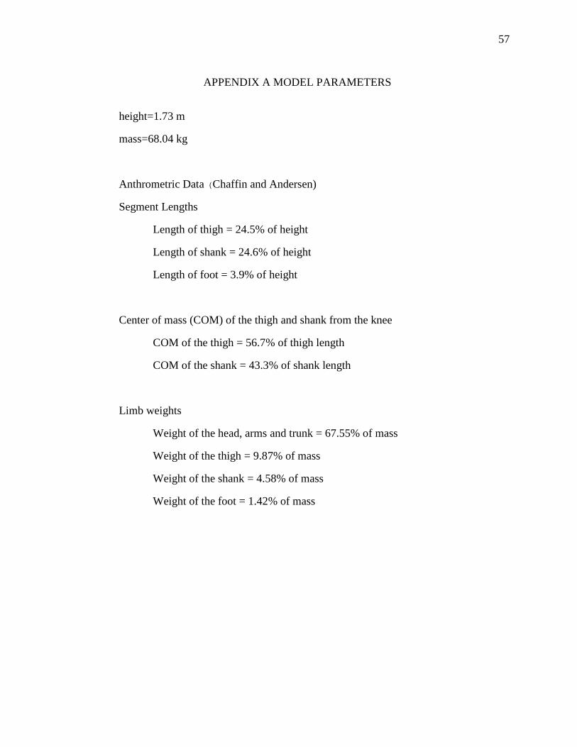
57

57

APPENDIX A MODEL PARAMETERS

height=1.73 m

mass=68.04 kg

Anthrometric Data (Chaffin and Andersen)

Segment Lengths

Length of thigh = 24.5% of height

Length of shank = 24.6% of height

Length of foot = 3.9% of height

Center of mass (COM) of the thigh and shank from the knee

COM of the thigh = 56.7% of thigh length

COM of the shank = 43.3% of shank length

Limb weights

Weight of the head, arms and trunk = 67.55% of mass

Weight of the thigh = 9.87% of mass

Weight of the shank = 4.58% of mass

Weight of the foot = 1.42% of mass

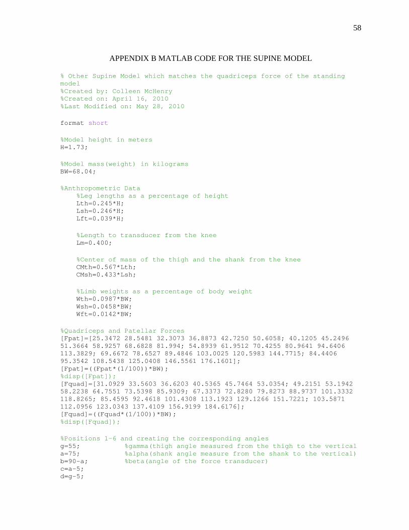
58

58

APPENDIX B MATLAB CODE FOR THE SUPINE MODEL

% Other Supine Model which matches the quadriceps force of the standing model %Created by: Colleen McHenry %Created on: April 16, 2010 %Last Modified on: May 28, 2010 format short %Model height in meters H=1.73; %Model mass(weight) in kilograms BW=68.04; %Anthropometric Data %Leg lengths as a percentage of height Lth=0.245*H; Lsh=0.246*H; Lft=0.039*H; %Length to transducer from the knee Lm=0.400; %Center of mass of the thigh and the shank from the knee CMth=0.567*Lth; CMsh=0.433*Lsh; %Limb weights as a percentage of body weight Wth=0.0987*BW; Wsh=0.0458*BW; Wft=0.0142*BW; %Quadriceps and Patellar Forces [Fpat]=[25.3472 28.5481 32.3073 36.8873 42.7250 50.6058; 40.1205 45.2496 51.3664 58.9257 68.6828 81.994; 54.8939 61.9512 70.4255 80.9641 94.6406 113.3829; 69.6672 78.6527 89.4846 103.0025 120.5983 144.7715; 84.4406 95.3542 108.5438 125.0408 146.5561 176.1601]; [Fpat]=((Fpat*(1/100))*BW); %disp([Fpat]); [Fquad]=[31.0929 33.5603 36.6203 40.5365 45.7464 53.0354; 49.2151 53.1942 58.2238 64.7551 73.5398 85.9309; 67.3373 72.8280 79.8273 88.9737 101.3332 118.8265; 85.4595 92.4618 101.4308 113.1923 129.1266 151.7221; 103.5871 112.0956 123.0343 137.4109 156.9199 184.6176]; [Fquad]=((Fquad*(1/100))*BW); %disp([Fquad]); %Positions 1-6 and creating the corresponding angles g=55; %gamma(thigh angle measured from the thigh to the vertical a=75; %alpha(shank angle measure from the shank to the vertical) b=90-a; %beta(angle of the force transducer) c=a-5; d=g-5;

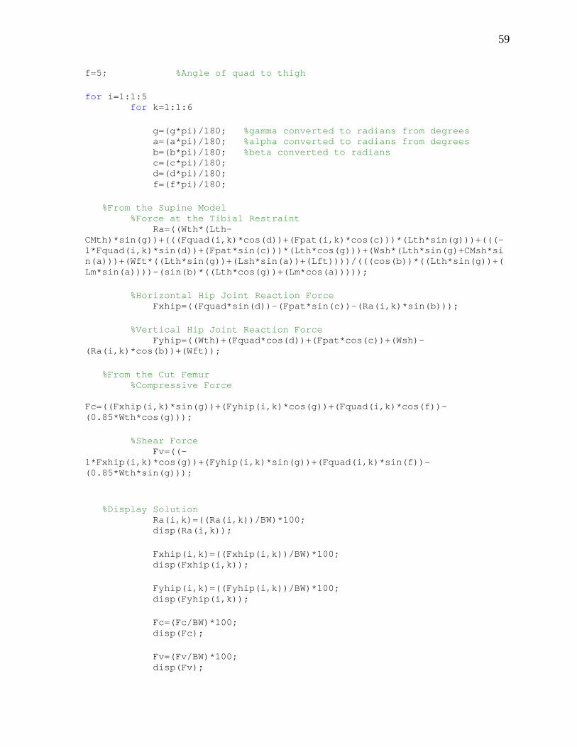
59

59

f=5; %Angle of quad to thigh for i=1:1:5 for k=1:1:6 g=(g*pi)/180; %gamma converted to radians from degrees a=(a*pi)/180; %alpha converted to radians from degrees b=(b*pi)/180; %beta converted to radians c=(c*pi)/180; d=(d*pi)/180; f=(f*pi)/180; %From the Supine Model %Force at the Tibial Restraint Ra=((Wth*(Lth-CMth)*sin(g))+(((Fquad(i,k)*cos(d))+(Fpat(i,k)*cos(c)))*(Lth*sin(g)))+(((-1*Fquad(i,k)*sin(d))+(Fpat*sin(c)))*(Lth*cos(g)))+(Wsh*(Lth*sin(g)+CMsh*sin(a)))+(Wft*((Lth*sin(g))+(Lsh*sin(a))+(Lft))))/(((cos(b))*((Lth*sin(g))+(Lm*sin(a))))-(sin(b)*((Lth*cos(g))+(Lm*cos(a))))); %Horizontal Hip Joint Reaction Force Fxhip=((Fquad*sin(d))-(Fpat*sin(c))-(Ra(i,k)*sin(b))); %Vertical Hip Joint Reaction Force Fyhip=((Wth)+(Fquad*cos(d))+(Fpat*cos(c))+(Wsh)-(Ra(i,k)*cos(b))+(Wft)); %From the Cut Femur %Compressive Force Fc=((Fxhip(i,k)*sin(g))+(Fyhip(i,k)*cos(g))+(Fquad(i,k)*cos(f))-(0.85*Wth*cos(g))); %Shear Force Fv=((-1*Fxhip(i,k)*cos(g))+(Fyhip(i,k)*sin(g))+(Fquad(i,k)*sin(f))-(0.85*Wth*sin(g))); %Display Solution Ra(i,k)=((Ra(i,k))/BW)*100; disp(Ra(i,k)); Fxhip(i,k)=((Fxhip(i,k))/BW)*100; disp(Fxhip(i,k)); Fyhip(i,k)=((Fyhip(i,k))/BW)*100; disp(Fyhip(i,k)); Fc=(Fc/BW)*100; disp(Fc); Fv=(Fv/BW)*100; disp(Fv);

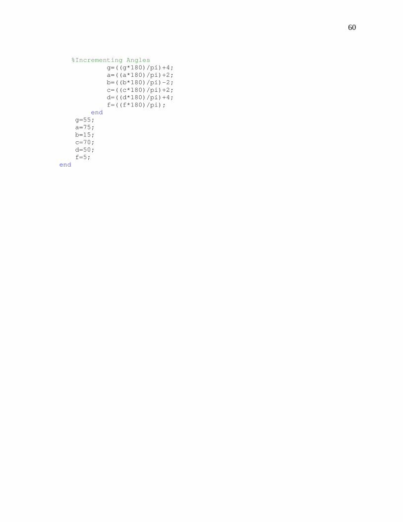
60

60

%Incrementing Angles g=((g*180)/pi)+4; a=((a*180)/pi)+2; b=((b*180)/pi)-2; c=((c*180)/pi)+2; d=((d*180)/pi)+4; f=((f*180)/pi); end g=55; a=75; b=15; c=70; d=50; f=5; end

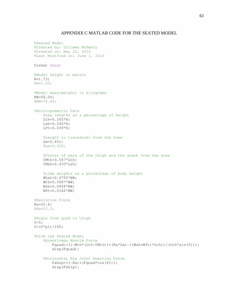
61

61

APPENDIX C MATLAB CODE FOR THE SEATED MODEL

%Seated Model %Created by: Colleen McHenry %Created on: May 22, 2010 %Last Modified on: June 1, 2010 format short %Model height in meters H=1.73; %H=1.93; %Model mass(weight) in kilograms BW=68.04; %BW=70.45; %Anthropometric Data %Leg lengths as a percentage of height Lth=0.245*H; Lsh=0.246*H; Lft=0.039*H; %Length to transducer from the knee Lm=0.451; %Lm=0.320; %Center of mass of the thigh and the shank from the knee CMth=0.567*Lth; CMsh=0.433*Lsh; %Limb weights as a percentage of body weight What=0.6755*BW; Wth=0.0987*BW; Wsh=0.0458*BW; Wft=0.0142*BW; %Resistive Force Ra=20.8; %Ra=13.3; %Angle from quad to thigh f=5; f=(f*pi)/180; %From the Seated Model %Quadriceps Muscle Force Fquad=(((-Wth*(Lth-CMth))+(Ra*Lm)-((Wsh+Wft)*Lth))/(Lth*sin(f))); disp(Fquad); %Horizontal Hip Joint Reaction Force Fxhip=((-Ra)+(Fquad*cos(f))); disp(Fxhip);

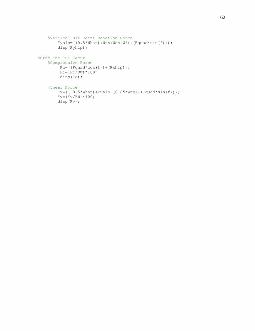
62

62

%Vertical Hip Joint Reaction Force Fyhip=((0.5*What)+Wth+Wsh+Wft+(Fquad*sin(f))); disp(Fyhip); %From the Cut Femur %Compressive Force Fc=((Fquad*cos(f))+(Fxhip)); Fc=(Fc/BW)*100; disp(Fc); %Shear Force Fv=((-0.5*What)+Fyhip-(0.85*Wth)+(Fquad*sin(f))); Fv=(Fv/BW)*100; disp(Fv);