A Bayesian network structure for operational risk ... · A Bayesian network structure for operational risk ... of Accounting and Finance, Monash University, ... Introduction. Banks

WORKING PAPER (Part 1.1)

1

A Bayesian network structure for operational risk

modelling in structured finance operations.

Andrew D. Sanford1 and Imad A. Moosa.

Department of Accounting and Finance

Faculty of Business and Economics

Monash University, Australia

Working Abstract: It is only recently that banks have begun to take seriously the

measurement and management of operational risks. The inclusion of operational risk

within Basel II is evidence of its increased importance. Although much previous

research into operational risk has been directed at methods for determining levels of

economic capital, our research is concerned more locally with the of an operational

risk manager at a business unit level. The business unit level operational risk manager

is required to measure, record, predict, communicate, analyse and control the

operational risks within their unit. It has been proposed by a number of finance

researchers that Bayesian Network models may be practical tools in supporting the

risk manager’s role. In the following research, we take the first steps in developing a

Bayesian network structure to support the modelling of the operational risk. The

problem domain is a functioning structured finance unit within a major Australian

bank. The network model incorporates a number of existing human factor frameworks

to support the modelling of human error and operational risk events within the

domain. The network supports a modular structure, allowing for the inclusion of many

different operational risk event types, making it adaptable to many different

operational risk environments.

Keyworks: Operational risk, Human Error, Bayesian networks.

1 Corresponding Author. Email: [email protected]. The authors would also like

to acknowledge the financial support provided through two research grants awarded by the Department

of Accounting and Finance, Monash University, and the Melbourne Centre for Financial Studies.


2

1. Introduction.

Banks and non bank financial institutions (NBFI) have become increasingly complex

organizations in terms of size and scope, global reach, and product and technological

complexity. In addition to their more traditional concerns with credit and market risk,

these factors have driven the need for such organizations to become more aware of the

operational risks they face. Although severe operational risk events are very rare, such

events have demonstrated their potential to bankrupt an organization (Barings Bank,

1995).

Operational risk is defined by the Basel Committee working paper (BCBS

2001) as ‘the risk of loss resulting from inadequate or failed internal processes, people

and systems or from external events’. This definition covers legal risk, or risk

associated with legal action, but does not include reputational risk (loss due to a

decline in a firm’s reputation) or strategic risk (loss associated with a failed strategic

direction). The Basel Committee defines seven types of operational risk, external

fraud; internal fraud; damage to physical assets; clients, products and business

practices; business disruption and system failure; execution, delivery and process

management; and employment practices and workplace safety. In this research, the

type of operational risk modelled falls under ‘execution, delivery and process

management’.

Bayesian networks have been recommended (Alexander (2000, 2003), Mittnik

and Starobinskaya (2007), and more recently by Moosa (2008)) as a tool for

measuring and managing operational risk in financial organizations. The inherent

heterogeneity and limited availability of operational risk event data makes modelling

is more problematic than the traditionally risk categories such as credit and market

risk. Both of these established risk categories have the advantage of large historical

data sets of comparatively homogenous data. Operational risk modelling therefore

includes the need to augment the sparse, historical, operational risk event data with

human judgement and expert opinion. Expert elicitation is an important input into the

construction of the Bayesian network structure developed in this research.


3

2. Literature Review.

Although new to the banking and finance industry, it could be argued that modelling

operational risks using probabilistic network models, such as Bayesian networks, has

been around for quite some time. Similar models have been developed in other

industrial settings, often under the label of Probabilistic Risk Analysis (PRA) (See

Bedford and Cooke, 2001). This form of analysis, which has evolved out of

engineering based practice, has until recently been more commonly applied to

industrial situations as found in nuclear energy, aerospace and chemical processing,

rather than commercial contexts. Paté-Cornell and Dillon (2006) define PRA as the

combination of systems analysis and probabilistic elicitations tools. The typical

common tools used in PRA being fault and event trees, which provide causal

descriptions of operational risk events. Although Bayesian network tools have been

applied to PRA analysis in industry, it is our view that the technology is particularly

well suited to operational risk modelling in commercial contexts. Whilst the logic

based fault and event trees models are more suited to modelling the ‘hard’ physical

and technical environments found in industry, Bayesian networks are more apt at

modelling the ‘conceptual’ and ‘subjective’ environments found within the ‘softer’

commercial context. Modern commercial activities are highly dependent on human

and systems reliability, as well as the human-to-human and human-to-computer

interfaces. Bayesian networks are particularly suited to modelling these areas given

the tools ability to fuse disparate and diverse historical and subjective data. This

makes it in our view a better modelling tool than the more logic-driven fault and event

trees, for the commercial environment.

The underlying technologies that make Bayesian network tools possible have been

available now for twenty years (Pearl, 1988; Neapolitan, 1990). A very diverse range

of literature now exists that describes the application of Bayesian networks to a

multitude of domains. A short, but by no means exhaustive list of published

applications include; transportation (Trucco, Cagno, Ruggeri and Grande, 2008);

systems dependability (Sigurdsson, Walls and Quigley, 2001; Neil, Tailor, Marquez,

Fenton and Hearty, 2008); infrastructure (Willems, Janssen, Verstegen and Bedford,

2005); medical and health care provision (van der Gaag, Renooij, Witteman, Aleman

and Taal, 2002; Cornalba, 2009); environmental modelling (Bromley, Jackson,

Clymer, Giacomello and Jensen, 2005; Uusitalo 2007); legal/evidential reasoning


4

(Kadane and Schum (1996)), forensic science (Taroni, Aitken, Garolino and

Biedermann, 2006), venture capital decision making (Kemmerer, Mishra, and Shenoy,

2002), project management (Khodakarami, Fenton and Neil, 2007), customer service

delivery (Anderson, Mackoy, Thompson and Harrell, 2004), new product

development (Cooper, 2000), traffic accident modelling (Davis, 2003) and national

security and terrorist threats (Paté-Cornell and Guikema, 2002). A common

underlying theme of many of these works is the development of models to facilitate

reasoning and decision making under uncertainty.

Papers concerned specifically with operational risk modelling within the finance

industry using Bayesian networks are limited, with a relatively short history. These

include Neil, Fenton and Taylor (2005), Mittnik and Starobinskaya (2007), Adusei-

Poku, van den Brink and Zucchini (2007), Cowell, Verrall and Yoon, (2007), and

Neil, Häger and Andersen (2009). None of these papers, with the exception of

Adusei-Poku et al (2007), base their models on ‘real-world’ banking environments.

Neil, Fenton and Taylor (2005) describe the use of a Bayesian network to model

statistical loss distributions for operational risk in financial institutions. Their

emphasis is on what they describe as the core problem of predicting losses. They

describe the Bayesian networks as providing further support for self-assessment

oriented scorecards. Bayesian networks suggest Neil et al (2005), provide the ability

to combine proactive loss indicators, with reactive outcome measures including loss

and near miss events, incorporate of expert judgment and qualitative estimates,

provide graphical representation and documentation, and inference over incomplete

observations, and which provides predictive, verifiable, outputs. They produce a

model using the Loss Distribution approach (LDA), basing total operational risk

losses on combining event frequencies and event severities. From the total loss they

determine the expected and unexpected losses as defined under Basel definitions.

They also introduce as parent nodes of the frequency and severity nodes, a process

effectiveness node, which also has parents that represent operational quality,

technological fidelity and staff quality. The introduction of these risk drivers

demonstrates a movement away from using these models for purely capital allocation,

to managing the causes of operational risk events.

Adusei-Poku, van den Brink and Zucchini (2007) develop a Bayesian network

model of operational risk in an operational FX settlement domain. With a similar goal

to our own, Adusei-Poku et al are concerned with developing an operational risk


5

management tool rather than a model for determining economic capital allocation.

They begin by describing the process of FX settlement and in identifying the sub-

processes that are entailed. They define each operational risk event in the FX

settlement process, which include, delayed payments, incorrect payments, misdirected

payments, non-payments and duplicate payments. The model they develop is based

also on the LDA common with operational risk models, as previously described in

Neil et al (2005) whereby the frequency of operational risk events is modelled

separately to the severity of events. The final operational risk distribution is generated

as a convolution of the two. The entire parameterization of the model was based on

domain expert elicitations, carried out using formal methods. Despite the availability

of historical data, it appears that Adusei-Poku et al (2007) took no opportunity to use

any model learning features of the Bayesian network tool. Although the FX settlement

environment appears similar to our own, it differs in that it involves a more

homogenous set of transaction types and processes, which allows more of these

processes to be automated. This results in less reliance on ‘ad-hoc’ human processing

arrangements and the subsequent exposure to human error. Having said this however,

the type of error causes sound remarkably similar to the analysis in our own research.

Adusei-Poku et al (2007) identify causes of settlement failures to be quality of

settlement information and payment input method, which although not identical, have

similar features to our own identified causes as data integrity and transaction

implementation errors found in our analysis cited in this research.

Cowell, Verrall and Yoon (2007) provide a comprehensive discussion of two

fictional applications of Bayesian networks. The first scenario involves modelling

operational risk events associated with computer systems failures of an e-business,

whilst the second models fraudulent claims in the insurance business. Cowell et al

(2007) demonstrate how Bayesian networks can be used to i) form posterior

probabilities of events given observations on other states of the domain, ii) simulate

different scenarios for each business line, iii) adapt or learn new probabilities for

events and iv) quantify the predictive performance of each model. Cowell et al (2007)

note that a drawback of Bayesian networks as a modelling tool is that they can require

considerable initial resources to setup. They also note that although a strength of

Bayesian networks is its subjective nature, this attribute is also a weakness in having

them accepted by prudential supervisors for the purpose of measuring risk capital

allocations. We particularly agree with the second view, and as such, have


6

concentrated our model purely on the need for institutions to internally manage their

operational risk profile.

Mittnik and Starobinskaya (2007) look at using Bayesian networks as a solution

for the Advanced Measurement Approach put forward in Basel II. Their concern is

that standard methods of modelling stochastic dependencies are insufficient for

assessing operational risk. Conventional models use correlations or copulas to

measure the relationships between business lines and risk events but do not include

measures of causal relationships between these entities. Mittnik and Starobinskaya

(2007) also follow the LDA specified under Basel II, modelling the frequency and

impact of operational risk events separately. They argue that ignoring topological

aspects of the domain as regards the interconnection of work-processes and

information flows means that standard models do not adequately account for multiple,

simultaneous failures. Applying Monte Carlo simulation, they demonstrate that at

different degrees of dependency, the topological interconnections between business

lines result in an avalanche-like effect, or clustering of events.

Neil, Häger and Andersen (2009) develop a hybrid dynamic Bayesian network for

the modelling of operational losses faced by financial institutions for the purposes of

economic capital allocation. The authors claim that applications of Bayesian networks

have failed to address three fundamental problems, i) application thus far have only

been applied to small fragments of a much more complex banking environment, ii)

models have not incorporated the time dynamics of operational risk events, and iii)

implementation of continuous variables. As in Neil et al (2005), the authors create a

model involving three layers, one for modelling operational risk events, another for

operational risk impact and a third for the aggregation of losses. The model developed

is a hybrid model, containing both discrete and continuous nodes. The authors model

the interactions between failure modes and controls, to generate an approximate

continuous loss distribution using an algorithm they call dynamic discretization. This

algorithm determines the discretization of continuous nodes automatically. This

avoids the trial-and-error approach required by modellers to manually select the

appropriate discretization ranges, which may changes as distributions in the

environment change.

In the following sections we discuss Bayesian network technology in more detail.

We then follow this with a description of the structured finance operations domain,

highlighting the important issues within the environment, as they affect operational


7

risk events. We discuss the methodology of Bayesian network development,

emphasizing the structural development component, going on to then describe our

model in detail. We then complete the paper with our conclusions.

3. Bayesian Networks.

Another detailed presentation of Bayesian Network technology2 seems unnecessary

given the large number of very good references currently available. (See Jensen and

Neilsen, 2007; Korb and Nicholson, 2004; Neapolitan, 2004). We provide therefore

only a brief description of the technology, to give sufficient background for the

remainder of the paper. For a more comprehensive discussion of Bayesian networks,

as they relate to Operational Risk modelling, refer to Cowell, Verrall and Yoon

(2007).

A Bayesian network consists of nodes and directional arcs or arrows. Each node

may be either discrete, having at least two states, or continuous, with a Gaussian

distribution over the real line. Within the Bayesian network, each node represents

some variable of interest within the domain being modelled. Behind each node is a

function that represents the probability distribution of the states of that node. Often

that function is represented as a table, which is called the conditional probability table

(or CPT), or node probability table (NPT). Given the semantics of the nodes and

states, we see that in modelling an environment, the modeller must decide on what

variables are of interest to the user or decision maker. They must also decide on what

measures are used to determine the state of these variables and what state descriptors

provide the most value to the user or decision maker. In determining the number of

states for a discrete node, the modeller should be aware that increasing the states will

improve the granularity of the measure, but will make probability elicitation

potentially more complex. A trade off therefore, between the number of states, and the

additional complexity needs to be considered when developing the network.

More contentious has been the meaning of the directed arcs within a Bayesian

network model. It is usually the case however, that arrows and their direction encode

2 The Bayesian network technology has been available for twenty years, and so a large number of tools,

in both a commercial and research-based form, are now available for research, development and

applications. The tool used for this research was Hugin Researcher v7.0.


8

a concept of ‘influence’ or ‘cause’ within the domain. An arrow extending from node

X to node Y indicates that a change in or manipulation of the state of node X will

cause changes in the state of node Y. In our paper, we take the firm view that the

arrow directions are causal.

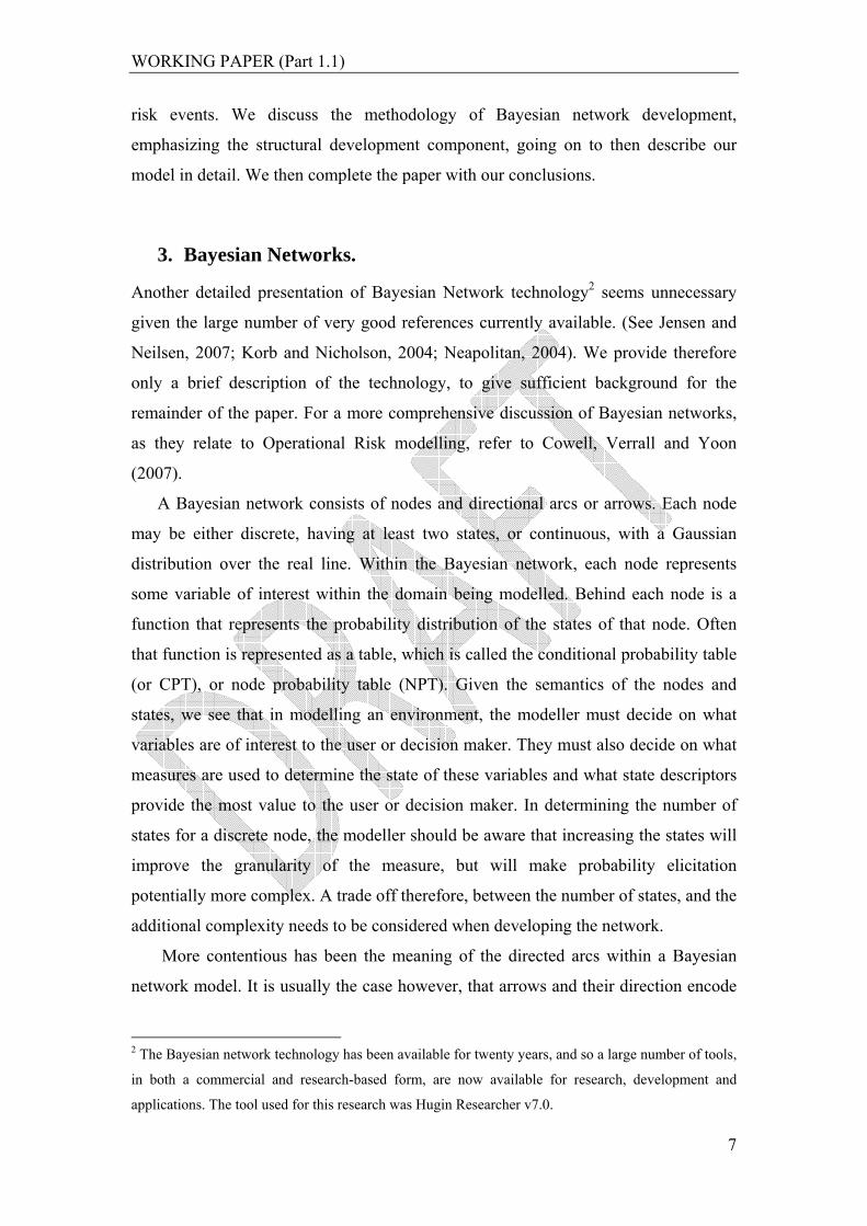
Architecturally, although Bayesian networks can take on an arbitrary level of

complexity, all models consist of three basic structures. These are the serial,

convergent or divergent structures, as illustrated in Figure 1. Although networks can

be constructed whereby all nodes are connected to each other, Bayesian networks are

more suitable as a modelling tool in situations where connections between nodes are

sparse rather than saturated.

Figure 1: Network components. From left to right, serial, divergent and convergent structures.

Once the nodes and causal relationships are identified, and the Bayesian network

constructed, the state probabilities can then be elicited and incorporated into the nodes

CPTs. These state probabilities can be elicited from human experts, statistical analysis

of historical data, or in some situations, learned directly by the Bayesian network.

After state probabilities have been included, the network can then be queried by

the user. In querying the network, information or evidence regarding the state of the

domain is usually entered. This evidence is propagated throughout the network,

allowing the marginal distributions of unobserved states within the environment to be

determined, based on the assumptions encoded in the model. Before any evidence is

entered, a node X will display its a priori marginal distribution, Pr(X). After evidence


9

ε has been entered into the network, the unobserved nodes such as X, will then display

their a posteriori distribution Pr(X | ε).

One of the advantages of using a Bayesian network as a modelling tool is that it

can answer queries that are both predictive and diagnostic. For example, a predictive

query may ask “what is the probability of a payment failure given that a loan is being

processed?”, whilst a diagnostic query may ask, “what is the most probably

transaction type processed given that a payment failure occurred?”. Therefore, having

observed the state of an effect node, such as a payment failure, inference can be

carried out to show the probable states of the causal nodes within the network.

4. Structured Finance Operations.

The bank involved is one of Australia’s largest domestic banks. Included within the

group is the bank’s wholesale banking division, which itself also includes two

business units, the Structured Finance and Corporate Finance units. It is the

responsibility of these two units to develop and market structured finance products to

the banks wholesale corporate customers. Structured products are created by bundling

individual transaction products together to provide a tailored financial solution to

meet an individual clients needs. The different individual products that may be

included within a structured product can range from simple vanilla loans and deposits,

to the more complex risk management tools such as OTC Options and Credit

Derivatives. Such structure products may have overall terms lasting as little as two

weeks, to as long as five years. They may be comprised of only a few individual cash

flows involving only a single currency, or a large number of flows involving different

currencies, values and timings. These structured products may also involve the

establishment of alternative legal structures or Special Purpose Vehicles (SPVs)

necessary to make the transactions tax-effective. To manage these complex

transactions during the life of each structured product, a separate business unit has

been established within the wholesale banking division. This unit, which we will refer

to as Structured Finance Operations (SFO), is responsible for the successful

implementation of each structure finance product.

The management and staffing of SFO consists of a single Director, who has

overall responsibility for the leadership of SFO, its budgets, workflow and personnel.

A number of Associate Directors, reporting directly to the Director, are responsible


10

for the day-to-day management of SFO deal teams. They also have direct

responsibility for any individual deals of a highly complex nature. Below them are the

Associates, or line managers, who take responsibility for a number of outstanding

individual deals, and who direct the Analysts which are junior operational staff within

the deal team. It is the Analysts who perform most of the activities related to the

individual transactions. Given the diversity of transaction types within the domain,

SFO operators tend to be generalists rather than specialists. For this reason, SFO

management have found difficulty in replacing staff once they move on to other areas

of the bank. This creates further potential risks brought on by staff turnover, the

adequacy of staff training, and the level of task instruction necessary.

Given the heterogeneity of the different transaction types making up a structured

product, it is difficult to develop a process based work model to manage them.

Instead, SFO’s has had to implement a ‘Deal Team’ or jobbing arrangement. Such a

structure provides the flexibility to implement the actions necessary to support these

bespoke products. This flexibility is not costless however, with the potential for more

frequent operational risk events resulting from human error. Furthermore, much of the

bank’s existing, automated legacy systems, lack the specific functionality needed to

support these unique products. Therefore the greater reliance on both manual and

spreadsheet-based solutions has resulted, more so, than in a homogenous transaction

environment.

In the process of creating a new structured product for a client, the Structured

Finance and Corporate Finance units produce a physical document known as the

‘Deal Document’. Within this document, all details such as transactions types, cash

flows, timings, currencies, and legal structures are specified and described. The deal

document is the ‘blue print’ that specifies the structured product from initial setup to

termination. It is the deal document that is passed to SFO, and it is the deal document

on which SFO staff relies to guide them through each transaction. Given the potential

complexities and risks involved with structured products, considerable due diligence

is carried out in the authoring of this document. The document passes through a large

number of oversight hurdles prior to its release to SFO, to ensure that any errors are

removed.

From an operational risk perspective and as defined under Basel II, SFO exposes

the bank to ‘Execution, Delivery and Process Management’ risks. SFO has identified

its major operational risks as


11

• Payments made to incorrect beneficiaries, and/or for an incorrect amount,

and/or for an incorrect value date.

• Regulatory breach, such as regulatory reporting or account segregation.

• Failure to enforce its rights or meet its obligations to counterparties over the

life of a deal.

• Exposure capture. This is the risk that the terms of a transaction or details

of a counterparty/security are not accurately recorded in the Bank’s

systems, resulting in a misunderstanding of the risk profile.

Other risks also identified by SFO, include ‘Approval Compliance’; the risk that

transactions are undertaken without the necessary internal approval process,

‘Documentation’; the risk that documentation does not adequately protect the Bank’s

rights because of incorrect execution or incorrect drafting, and ‘Theft’; the risk that

bank or customer funds or property are misappropriated.

As part of the existing operational risk oversight and assessment of SFO, Business

Environment Scorecards are prepared regularly. These identify generic key risk

drivers (KRDs) common to all units within the wholesale banking division and score

individual units against each dimension. These generic risk drivers include; i) whether

the unit is large and distributed or small and centralized; (‘Scale’ measure); ii)

whether transactions processed within the unit are of a large wholesale dollar

amounts, or low retail dollar values; (‘Transaction’ measure); iii) whether the

products are complex, and large in volume or simple and low in volume. (‘Product’

measure); iv) whether the operational processes within the unit are complex, manual

and outsourced, or simple, automated and carried out in-house; (‘Process’ measure);

v) whether the units operational and systems technology is legacy, disparate and with

multiple interfaces, or is modern, integrated and with fewer interfaces; (‘Technology’

measure); vi) whether unit staff are incentive driven, with high turnover, or wage and

salary remunerated with low turnover; (‘Staff measure); vii) whether the unit is

undergoing rapid, large scale and complex change, or slow, small scale and simple


12

change; (‘Change’ measure); viii) whether the unit is experiencing new aggressive

and competitive entrants, or whether competition is benign and stable; (‘Competition’

measure); (ix) whether the unit operates in a tight regulatory environment, with

multiple legal entities and global reach, or whether the unit has a loose regulatory

environment, with few legal entities and a local or national focus;

(‘Regulatory/Legal/Geographic’ measures). For each unit, the operational risk drivers

are rated a number from 1 (highest risk) to 9 (lowest risk). Although scorecards are a

popular and valuable tool, unlike Bayesian networks, they do not make explicit the

causal relationships between various risk drivers.

SFO senior management view the Bayesian network model as offering a number

of practical features. Firstly, the risk communications within and across business units

will be improved, as the model will make explicit the risk drivers and their causal

relationships. Furthermore, auditable justifications for risk decisions will be made

explicit and accessible to external parties. For example, the model could be used to

support the bank’s internal audit team in assessing the risk profile of SFO. The model

will also provide supporting evidence for management decisions on reducing and

mitigating potential operational risks within the business unit. Although the model in

this paper will not incorporate decision nodes, the Bayesian network technology

readily allows for the inclusion of decision, as well as utility nodes, and these may be

added in future version of the model.

5. Methodology

Whilst efficient algorithms for inference in Bayesian networks have been available for

some time, construction and development of these networks is still as much art as it is

science. In modelling a problem domain, the developer must use their judgement in

determining what level of detail is appropriate, which nodes should be included, and

what causal relationships may exist. Supporting these choices is the ultimate purpose

of the model. As a simple modeling rule, choices made have been informed by our

desire to provide potential users with gainful insights of the domain, whilst at the

same time, avoiding the creation of a model whose complexity made future use

cumbersome and difficult to maintain and improve. Pragmatically, the rule has been,

‘Simple enough to be used and complex enough to be useful’. The development

approach is taken from the knowledge elicitation methodology discussed in Korb and

Nicholson (2004). This methodology emphasizes the use of domain experts in the


13

construction and elicitation phases, with iterative feedback and re-modelling being an

important feature.

Reliance on human expert judgement in the construction and elicitation phases

presents a number of difficulties. These include such situations whereby the available

domain experts do not have sufficient knowledge scope to cover all facets of the

domain, or where domain experts have difficulty specifying the correct causal

orderings of events, or where problems associated with the combination of different

probabilities provided by all of the individual experts arise. A potential remedy for

such difficulties is the use of automated machine learning techniques, which have

been an active area of Bayesian network research, motivated particularly by the desire

to overcome the bottleneck associated with using expert judgement. Many Bayesian

network tools incorporate such machine learning algorithms, including the tool used

in this research. Given the lack of available ‘hard’ observational data, domain expert

input appears unavoidable in our specific research. More generally, this may always

be somewhat true, given the very nature of operational risk. Despite these difficulties,

it is our view that with regards to operational risk management; the involvement of

domain experienced expert judgement is very desirable. Incorporation of expert

knowledge is therefore a strength of Bayesian network modeling, as well as ironically

a weaknesses, because of the difficulties expert elicitation presents.

The Bayesian network construction process is iterative; proceeding in steps and

cycles. The following development steps are drawn from Korb and Nicholson (2004);

1. Structural Development and evaluation. Initial development proceeds by

identifying all the relevant risk driver events, their causal relationships, and

the query, hypothesis or operational risk event variables. This produces a

causal network without any elicited or learned probability parameters.

Evaluating the network at this step can be performed by carrying out a d-

separation analysis, and/or a clarity test using domain experts not directly

involved in the network construction.

2. Probability elicitation and parameter estimation. This step involves defining

the probability distributions of the nodes and setting their parameter values.

Parameter values must be set such that they reflect the marginal and

conditional probabilities observed in the domain. Such marginal and


14

conditional distributions can be determined by reference to domain based

experimental results, passive observation of events, learning from historical

data, or access to domain experts. For our purposes, the last source dominates.

3. Model Validation. This step is probably the most problematic component of

the Bayesian network construction, especially when historical data is sparse.

How does one validate a model constructed largely through the subjective

opinion of experts? Korb and Nicholson (2004), suggest a number of

validations approaches including i) an elicitation review; ii) sensitivity

analysis; and iii) case evaluation. We incorporate the first two approaches to

validation of the model.

For the purposes this paper, we are only concerned with the first stage of the

development cycle, ‘Structural Development and Evaluation’, the remaining stages,

two and three, are discussed in Sanford and Moosa (2009).

Structure Development.

In the process of constructing the network model, we sought to answer the

following broad based questions.

• What operational risk queries should the model be able to answer?

• What operational risks categories and events should be included in the

model?

• What are the main risk drivers in SFO for operational risk events?

• What are the causal relationships between risk drivers and risk events?

• What are the key performance indicators for the SFO domain?

Acquiring answers to these initially proceeded through review of SFO’s internal

documentation to gain an appreciation of the business and operational environment.

The existing operational risk documents pertaining to SFO, provided by senior

operational risk staff, were of particular value. Included within this material were the

most recent Business Environment Score ratings for SFO. These scorecard

assessments proved invaluable in providing an overview of the unit’s operational risk

profile. SFO’s ratings were Scale - 8; Transactions - 2, Product - 2, Process - 2,

Technology - 4, People - 8, Change - 4, Competition - 8, Regulatory/Legal/Geography


15

- 7. Obviously from these ratings, Transactions, Products and Processes, as well as

Technology and Change present the greatest challenges to SFO. It has low transaction

volumes but with relatively high dollar values. Its products are relatively complex

whilst its processes are reliant on human performance and manual intervention. It also

faces a business environment which is dynamic and changing due to business growth.

Existing internal documentation also revealed that the key performance indicator

(KPI) used by SFO senior management was the number of transactions process per

month.

Following on from the document reviews, a number of face-to-face unstructured

and semi-structured interviews were carried out with the Director of Quality

Assurance.. For future reference, we refer to this domain expert as the ‘the risk

manager’. The risk manager had over twenties years of banking experience, and was

responsible for the monitoring of SFO’s operational risk events. For this reason they

had considerable interest in the project and the development of the Bayesian network

tool, as it directly impact their own area of responsibilities. The risk manager had

considerable detailed knowledge of the SFO domain and was very familiar with

operational processes involved, the potential risks events, and their drivers. They did

not however have any experience in Bayesian networks or their development as a

decision support or risk management tool. In carrying out these interviews, we sought

responses to the following broadly based questions.

Taking a user’s perspective, the risk manager saw the model as providing

probability outputs for the various operational risk events, conditional on the

underlying characteristics of each type of transaction performed within SFO. It was

the risk manager’s view that SFO management required a more formal method of

assigning operational risk capital allocations for each transaction managed. The

current methods for doing this were somewhat ad-hoc, opaque and reliant on the

judgement of senior management. By introducing the Bayesian model, a more formal

and transparent decision making approach would be available, based on hard

evidence, as well as professional judgement. The model would at the very least make

the cognitive causal models, used implicitly by SFO staff, accessible to internal and

external parties. The network model would also be useful as a baseline, negotiating

position, in discussions between SFO and any of the other transaction originating

business units.


16

During these interviews, several candidates were discussed as potential output

categories. The most important risk events to be included in the model, referred to as

the key risk indicators (KRI), were identified as payment failures, exposure

management failures and the regulatory/legal/tax failures. Payment failures included

any events related to a failed payment such as a payment delay caused by an incorrect

counterparty, incorrect value date, or incorrect payment amount. Exposure

management failures referred to any situations in which the banks financial positions

or risk exposures were incorrectly recorded. And finally, the regulatory/legal/tax

failures related to errors that resulted in the bank failing to meet it regulatory, legal or

tax requirements as they impacted on prudential supervision, legal requirements from

both the banks and the clients perspectives or with regard to the tax effectiveness of

transactions, such as account segregation.

To manage and control operational risks, an understanding their causal

antecedents was a key first step. In the operational risk literature, these causes are

often referred to as the key risk drivers (KRDs). The KRDs identified during the

initial and subsequent interviews included i) the transaction type, ii) the data capture

mode or mechanism (whether manual/spreadsheet or bank legacy system) for

recording transaction information, iii) existence of SPVs, iv) the actively managed

transaction volume currently handled by SFO’s staff, v) the skills (or quality) of

existing SFO staff, vi) the availability of SFO staff, vii) the accuracy of transaction

information capture, viii) the correctness of transaction implementation, and ix) the

existing oversight controls currently performed by SFO staff. Later interviews also

added x) the failure or downtime of computer systems as a risk driver and xi) the

working environment. Validation of the initial network design was carried out using a

structured walk-through by a senior Operational Risk analyst. During the model walk-

through, the operational risk analyst was able to confirm the existing nodes and their

proposed causal relationships, as well make a number of valuable suggestions as to

the inclusion of other nodes. These additional inclusions emphasized legal and

taxation issues. These suggested additions were later discussed, confirmed and

approved by the risk manager for inclusion into the model.

The transaction type driver includes not only the transaction type itself, but more

broadly the implicit transaction processing involved in actioning that transaction type.

Transaction types processed by SFO include; Loans (LN), Deposits (DEP), Foreign

Exchange transactions (FX), Interest Rate Swaps (IRS), Cross-Currency Interest Rate


17

Swaps (XCS), Exchange Traded Derivatives (ETD), Over-the-Counter Options

(OOP), Over-the-Counter Credit Derivatives (OCD), Listed Equities (EQL), Unlisted

Equities (EQU), Preference shares (EQP), Financial Leases (FNL), or Operating

Leases (OPL). Each of these represents a separate transaction type state within the

model. Each instrument may consist of one or more separate payments flows between

counterparties, an acquisition or removal of a financial instruments position, or

creation or closure of a SPV. Each may be denominated in a number of different

currencies. Each of these transaction types will involve a variety of actions, actions

which may be common to many, or unique to only a few. The idea of transaction type

being a driver of risk is an attempt to capture the different operational risks inherent in

each transaction process or the task variation.

The data capture mode driver refers to the manner in which transaction

information is captured and stored. This has implications for the risk profile of any

one transaction. This driver is closely associated with the existence or otherwise of a

SPV associated with the transaction being processed. Transactions processed with an

associated SPV are more likely to have their data capture performed using manual and

spreadsheet based solutions, than via the banks existing information system

infrastructure, with its attendant automated features, error and reconciliation controls.

This is because the use of SPVs can make a transaction more complex, requiring

processing that is unique for that transaction.

Furthermore, transaction-based characteristic risk drivers also include the

transaction size or principal value, and the payment or cash flow sizes associated with

that transaction. These characteristics have particular influence on the impact of an

operational risk event as potential losses can be closely linked to these variables.

Taken together, transaction type, data capture mode, SPV, transaction size and

payment size, constitute what we broadly categorize as the transaction characteristics

that drive operational risk events.

The next set of drivers, actively managed transaction volumes, and quality and

quantity of operational staff, which we broadly classify as ‘Skills & Experience’,

attempt to capture the important states of SFO’s working environment. Actively

managed transaction volumes provide a proxy measure to the key performance

indicator (KPI) used in SFO, the number of transaction processed. By including the

actively managed transaction volumes within the model, we also gain some measure

of the demands of the working environment on operational staff. It is the interaction


18

of external factors as found in the social-working environment and the technical

environment, constituted in the transactions and processes, on operational staff that

drives the internal psychological states of the SFO operators. We consider the internal

and external states of the operational staff to be of particular importance in driving

operational risks events, because of SFO’s reliance on human factors.

In an attempt to formally capture the internal states of the operational staff as they

interacting with their contextual working and technical task environments, we include

within the model a number of nodes that represent three important internal states of

the working operational staff. These categories, stress load, mental effort load and

time load, are taken directly from the Subjective Workload Assessment Technique

(SWAT) framework originally developed by Reid and Nygren (1988). We do not

utilize the SWAT in its entirety, but rather borrow its operator load categories only.

This framework introduces the measures, each of which has discrete, three-tiered

states. Each state is provided with a description which assists the operator in

determining the level of time, mental effort and stress load they experience, whilst

performing a given task. (See Table 1 for a description of each state). The SWAT is a

particularly popular framework, providing good face validity for an operator’s

internal state. By implication, it is the combination of these three individual states that

induce an overall workload state. For our purposes, the workload state is determined

by a simple summation of the individual states.

Further to SFO’s reliance on human factors, we include into the network model

another set of nodes with the purposes of capturing, under a more formal

categorization, the different types of human errors that may generate or potentially

generate operational risk events. These nodes, and the human error categories they

represent, are taken from Reason’s (1990) generic framework for human error

categories. These categories are mistakes, slips, lapses and mode errors. The

definition of each is given in Table 1. All human errors can be categorized under one

of these categories. Our reasoning for including these categories is to support SFOs

efforts to ‘learn’ more about their working and operational environment over time.

Using a formal categorization of human errors may assist SFO to develop a greater

awareness of what type of errors occur and how, particularly as staff interact with the

task environment. Categorizing error will help raise the awareness of the different

forms and their attributes, improving communications and situation awareness. These

categories are quite generic, however specific SFO categories could also be


19

developed, or other human error categories. For example, a more detailed framework

related to spreadsheet error taxonomies is described in Powell, Baker and Lawson

(2008, 2009), and could be incorporated into the network, with the human error

categories being divided between spreadsheet based and non-spreadsheet based errors.

Furthermore, other error categories could be included, such as the commonly used

‘Errors of Commission’, which constitute errors occurring due to actions being taken

that should not have been, and ‘Errors of Omission’, which involve errors arising

from not performing actions that should be performed.

Although the incorporation of Reason’s and the SWAT frameworks improves the

analytical features of the network model, it does come at some small cost. It makes

expert elicitation more difficult, as it is unlikely that local experts within SFO have

every given any consideration to these types of categories, or view their environment

in these terms. They are likely to be unfamiliar with these human error categories or

operator loadings, even though they will be called upon to provide a priori

probabilities. In introducing these node categories, it is important that the local

experts are given sufficient instruction to understand them, and support in deriving

prior probabilities for them.

To provide further categorization to error outcomes, we have also introduced

‘Error Types’ that are more specific to SFO, but which could also be relevant in other

back office and operational environments. These errors types are i) ‘System Errors’,

ii) ‘Data Entry Errors’, iii) ‘Transaction Implementation Errors’, and iv) ‘Oversight

Control Errors’. The only one of these four that we consider to be exogenous is the

systems error. We consider systems errors to be beyond SFOs control, but still having

the potential to cause operational risk events that impact on SFO operations. It is

because of the exogenous nature of this risk, it has no KRDs associated with it as

parent nodes. It was included however to cover those operational risk events that may

originate from a systems failure. We have made the comment similarly, that although

not done with our current model, deal document error could also be included as

another exogenous error type similar to systems error.


20

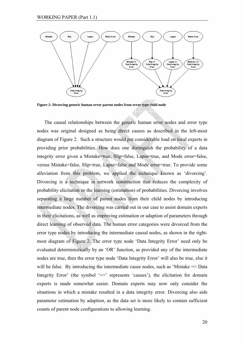
Figure 2: Divorcing generic human error parent nodes from error type child node

The causal relationships between the generic human error nodes and error type

nodes was original designed as being direct causes as described in the left-most

diagram of Figure 2. Such a structure would put considerable load on local experts in

providing prior probabilities. How does one distinguish the probability of a data

integrity error given a Mistake=true, Slip=false, Lapse=true, and Mode error=false,

versus Mistake=false, Slip=true, Lapse=false and Mode error=true. To provide some

alleviation from this problem, we applied the technique known as ‘divorcing’.

Divorcing is a technique in network construction that reduces the complexity of

probability elicitation or the learning (estimation) of probabilities. Divorcing involves

separating a large number of parent nodes from their child nodes by introducing

intermediate nodes. The divorcing was carried out in our case to assist domain experts

in their elicitations, as well as improving estimation or adaption of parameters through

direct learning of observed data. The human error categories were divorced from the

error type nodes by introducing the intermediate causal nodes, as shown in the right-

most diagram of Figure 2. The error type node ‘Data Integrity Error’ need only be

evaluated deterministically by an ‘OR’ function, as provided any of the intermediate

nodes are true, then the error type node ‘Data Integrity Error’ will also be true, else it

will be false. By introducing the intermediate cause nodes, such as ‘Mistake => Data

Integrity Error’ (the symbol ‘=>’ represents ‘causes’), the elicitation for domain

experts is made somewhat easier. Domain experts may now only consider the

situations in which a mistake resulted in a data integrity error. Divorcing also aids

parameter estimation by adaption, as the data set is more likely to contain sufficient

counts of parent node configurations to allowing learning.


21

The final categories are similar in to each other in structure and represent the

categories of operational risks events. These include Regulatory/Legal/Tax, Exposure

management and Payment failure events. Divorcing is also used between the error

types and the risk events, producing intermediate nodes, for example, the ‘Transaction

Implementation Error => Exposure Failure’ event. Divorcing was also done to ease

complexity, and aid, at a later stage of development, expert elicitation and improved

probability adaption.

One driver not included in the mix of KRDs has been the quality of the deal

document presented to SFO. Any errors in the deal document could be manifested

within the SFO environment as an operational risk event. To demarcate between units

we have assumed that the deal document received by SFO is completely correct. This

however is not a realistic assumption and is only used for the purposes of drawing a

boundary around SFO. The problem with this approach is that it removes the

opportunity for the bank to measure the correlations between operational risk events

occurring between units using the model. A failure in one unit manifests itself in

another unit. This is inconsistent with the current inclusion of the system failure KRD,

whose causal antecedents would likely be located in the wholesale banking division’s

information technology and systems management unit. It was Mittnik and

Starobinskaya (2007), critiquing current operational risk models, who suggested that

Bayesian networks represented superior modelling tools because they could more

easily incorporate the linkages between units.

Other operational risks events previously identified by SFO, such as 'Approval

Compliance’ and ‘Documentation’ are not explicitly included in the final network

model, although they may be included within ‘Regulatory/Legal/Tax failure’, at the

discretion of the risk manager. The subsequent modular design of the final network

however would make their inclusions relatively straightforward. As for the remaining

category ‘Theft’, we considered this category to be more problematic and requiring of

its own separate causal model.

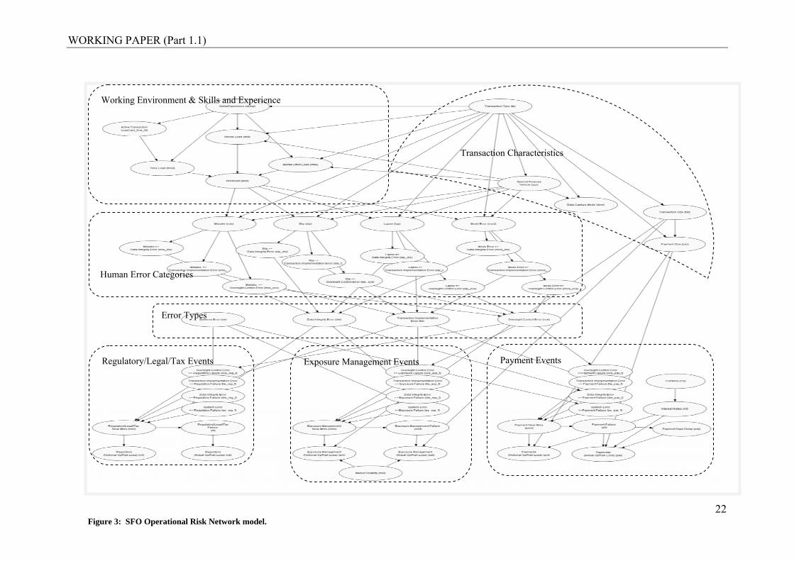
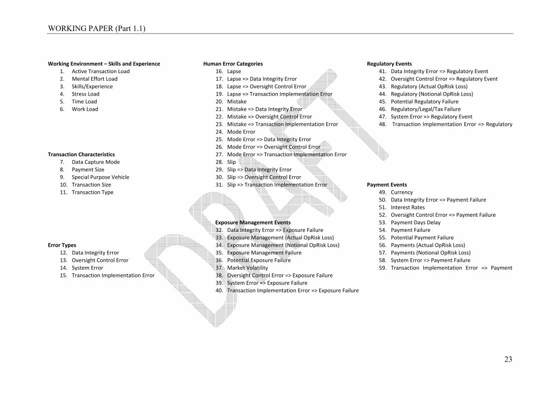
The structure of the final model is partitioned into the following broad categories.

These are described, i) Work Environment/Skills and Experience, ii) Transaction

Characteristics, iii) Human Error Categories, iv) Error Types, and the more familiar

operational risk events; v) Regulatory/Legal/Tax failure Events, vi) Exposure

Management failure Events, and vii) Payment failure Events.


22

Payment Events Exposure Management Events Regulatory/Legal/Tax Events

Human Error Categories

Error Types

Working Environment & Skills and Experience

Transaction Characteristics

Figure 3: SFO Operational Risk Network model.


23

Working Environment – Skills and Experience Human Error Categories Regulatory Events 1. Active Transaction Load 16. Lapse 41. Data Integrity Error => Regulatory Event2. Mental Effort Load 17. Lapse => Data Integrity Error 42. Oversight Control Error => Regulatory Event 3. Skills/Experience 18. Lapse => Oversight Control Error 43. Regulatory (Actual OpRisk Loss)4. Stress Load 19. Lapse => Transaction Implementation Error 44. Regulatory (Notional OpRisk Loss)5. Time Load 20. Mistake 45. Potential Regulatory Failure6. Work Load 21. Mistake => Data Integrity Error 46. Regulatory/Legal/Tax Failure

22. Mistake => Oversight Control Error 47. System Error => Regulatory Event 23. Mistake => Transaction Implementation Error 48. Transaction Implementation Error => Regulatory 24. Mode Error 25. Mode Error => Data Integrity Error 26. Mode Error => Oversight Control Error Transaction Characteristics 27. Mode Error => Transaction Implementation Error

7. Data Capture Mode 28. Slip8. Payment Size 29. Slip => Data Integrity Error9. Special Purpose Vehicle 30. Slip => Oversight Control Error10. Transaction Size 31. Slip => Transaction Implementation Error Payment Events 11. Transaction Type 49. Currency 50. Data Integrity Error => Payment Failure 51. Interest Rates

52. Oversight Control Error => Payment Failure Exposure Management Events 53. Payment Days Delay 32. Data Integrity Error => Exposure Failure 54. Payment Failure 33. Exposure Management (Actual OpRisk Loss) 55. Potential Payment FailureError Types 34. Exposure Management (Notional OpRisk Loss) 56. Payments (Actual OpRisk Loss)

12. Data Integrity Error 35. Exposure Management Failure 57. Payments (Notional OpRisk Loss)13. Oversight Control Error 36. Potential Exposure Failure 58. System Error => Payment Failure14. System Error 37. Market Volatility 59. Transaction Implementation Error => Payment 15. Transaction Implementation Error 38. Oversight Control Error => Exposure Failure 39. System Error => Exposure Failure 40. Transaction Implementation Error => Exposure Failure


24

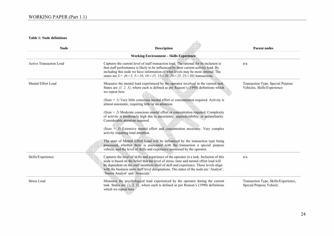
Table 1: Node definitions

Node Description Parent nodes

Working Environment – Skills Experience

Active Transaction Load Captures the current level of staff transaction load. The rational for its inclusion is that staff performance is likely to be influenced by their current activity load. By including this node we have information of what levels may be most optimal. The states are S = {0-<5, 5-<10, 10-<15, 15-<20, 20-<25, 25-<30} transactions.

n/a

Mental Effort Load Measures the mental load experienced by the operator involved in the current task. States are {1, 2, 3}, where each is defined as per Reason’s (1990) definitions which we repeat here. (State = 1) Very little conscious mental effort or concentration required. Activity is almost automatic, requiring little or no attention. (State = 2) Moderate conscious mental effort or concentration required. Complexity of activity is moderately high due to uncertainty, unpredictability, or unfamiliarity. Considerable attention required. (State = 3) Extensive mental effort and concentration necessary. Very complex activity requiring total attention. The state of Mental Effort Load will be influenced by the transaction type being processed, whether there is associated with the transaction a special purpose vehicle, and the level of skills and experience possessed by the operator.

Transaction Type, Special Purpose Vehicles, Skills/Experience

Skills/Experience Captures the level of skills and experience of the operator in a task. Inclusion of this node is based on the belief that the level of stress, time and mental effort load will be dependent on the staff members level of skill and experience. These levels align with the business units staff level designations. The states of the node are ‘Analyst’, ‘Senior Analyst’ and ‘Associate’.

n/a

Stress Load Measures the psychological load experienced by the operator during the current task. States are {1, 2, 3}, where each is defined as per Reason’s (1990) definitions which we repeat here.

Transaction Type, Skills/Experience, Special Purpose Vehicle.


25


(State = 1) Little confusion, risk, frustration, or anxiety exists and can be easily accommodated. (State = 2 ) Moderate stress due to confusion, frustration, or anxiety noticeably adds to the workload. Significant compensation is required to maintain adequate performance. (State = 3) High to very intense stress due to confusion, frustration, or anxiety. High to extreme determination and self-control required. The state of the stress load experienced by an operator will be dependent on the type of transaction being processed, the skills and experience the operator has, and whether the transaction complications associated with a special purpose vehicle are present.

Time Load Measures the time pressures experienced by the operator during the current task. States are {1, 2, 3}, where each is defined as per Reason’s (1990) definitions which we repeat here. (State = 1) Often have spare time. Interruptions or overlap among activities occur infrequently or not at all. (State = 2) Occasionally have spare time. Interruptions or overlap among activities occur frequently. (State = 3) Almost never have spare time. Interruptions or overlap among activities are very frequent, or occur all the time. The level of time load experienced by the operator will be dependent on their current active load and their skills and experience.

Active Transaction Load, Skills/Experience

Work Load Captures all aspects of mental effort, stress and time loads into single measure. The work load is simply the addition of all ratings for time, stress and mental effort load. States for Work Load are S = {Stress Load + Time Load + Mental Effort Load}. Give the states of the parent nodes, the Workload state will vary from 3 up to 9.

Stress Load, Time Load, Mental Effort Load.


26


Transaction Characteristics

Data Capture Mode Describes how transaction information is captured. The capture mode may be either manual, which includes the use of spreadsheets, or automatic, which indicates the use of a bank legacy computer system. The states are S = {‘Automatic’, ‘Manual’}. The capture mode will be influenced by the transaction type involved and whether a special purpose vehicle is use in the transaction.

Transaction Type, Special Purpose Vehicle.

Payment Size Identifies the payment amount in AUD currency. This is a discretized continuous variable. The numeric interval states are {Zero to AUD20million, AUD20million to AUD50million, AUD50 million to AUD100 million, AUD100 million to AUD250 million, AUD250 million to AUD500 million, AUD500 million to AUD1000 million, AUD1000+ million}. The currency node is a parent of the payment size. The assumption being that the currency in which the payment is made contains some information relevant to the size of the payment. For example, payments in US dollars may be generally larger than payments in Australian dollars.

Currency.

Special Purpose Vehicle Describes whether a special purpose vehicle is associated with a transaction. States are {false, true}. The parent node is transaction type. Transaction type is selected as a parent node as some transaction types are more commonly associated with special purpose vehicles.

Transaction Type.

Transaction Size Describes the transaction size in AUD currency. The transaction size is the principal amount involved for a transaction type. The numeric interval states are {Zero to AUD20million, AUD20million to AUD50million, AUD50 million to AUD100 million, AUD100 million to AUD250 million, AUD250 million to AUD500 million, AUD500 million to AUD1000 million, AUD1000+ million}. Transaction Type is a parent of transaction size as a transaction type influences the transaction size amount. Transaction type is the parent node as the transaction type involved will influence the respective transaction sizes.

Transaction Type.

Transaction Type Describe the transaction type. The states for transaction type are {LN, DEP, FX, IRS, XCS, ETD, OOP, OCD, EQL, EQU, EQP, FNL, OPL}. These states represent Loans, Deposits, Foreign Exchange transactions, Interest Rate Swaps, Cross-Currency Swaps, Exchange traded derivatives, Over-The-Counter Options, Over-

No parent nodes.


27


The-Counter Credit Derivatives, Listed Equities, Unlisted Equities, Preference shares, Financial Leases and Operating leases}. In the model, it is important to emphasize that the transaction type represents more than just the type of transaction involved. It more broadly represents the process required to record and implement that particular transaction type.

Error Types

Data Integrity Error Describes the event whereby an error or errors have been introduced into the recording of transactions, whether using a manual or automated system, which is considered by operational risk management to be material enough to cause an operational risk event. The states include {false, true}. The state is updated deterministically, being a function of the state of the parents. If any parent state is true, then this node will also be true.

Mistake => Data Integrity Error Slip=>Data Integrity Error Lapse => Data Integrity Error Mode Error=>Data Integrity Error.

Oversight Control Error Describes the event whereby an error or errors have been introduced into a process which are material enough to cause an operational risk event, and this error has been introduced because of an error in oversight control. Errors that would fall within the oversight control error category include, i) a failure in supervisory oversight, ii) failure in reconciliation procedures, iii) exceeding counterparty exposure limits, iv) exceeding authority. The states include {false, true}. The state is updated deterministically, being a function of the state of the parents. If any parent state is true, then this node will also be true.

Mistake => Oversight Control Error Slip=>Oversight Control Error Lapse => Oversight Control Error Mode Error=>Oversight Control Error.

System Error Describes the event that a systems error has occurred that is material enough to cause a potential operational risk event. A systems error include such events as a loss of systems due to, i) power failure, ii) software failure, iii) hardware failure, iv) computer virus, v) Denial of Service attach. The states include {false, true}. This node has no parents. It is considered that the parents of this node are situated outside of the SFO domain.

n/a

Transaction Implementation Error Describes the event that an error has been introduced in the implementation of a transaction that is material enough to cause an operational risk evernt. States are {false, true}.

Mistake => Transaction Implementation Error Slip=>Transaction Implementation


28


The state is updated deterministically, being a function of the state of the parents. If any parent state is true, then this node will also be true.

Error Lapse => Transaction Implementation Error Mode Error=>Transaction Implementation Error.

Human Error Categories

Lapse Describes whether a lapse error has occurred. A lapse error is defined as the failure to carry out an action. Lapses can be directly related to failures of memory. They are however different from knowledge-based mistakes associated with the overloading of the operators working memory, resulting in poor decision-making. Important lapses may involve the omission of steps in a procedural sequence. In this situation, an interruption is what often causes the sequence to be stopped, then restarted again a step or two later than it should have been. This definition of a lapse is taken from Reason (1990). States are {false, true}. The parent nodes being transaction type, work load and special purpose vehicle. These parents are considered to capture the major causes of human error, the transaction type processes, the complexity associated with special purpose vehicles and the environmental conditions that increase the operator’s workload.

Transaction Type, Work Load, Special Purpose Vehicle

Lapse => Data Integrity Error This allows for details as to the impact of the lapse error. In this case, the lapse error has caused a data integrity error. States are {false, true}.

Lapse

Lapse => Oversight Control Error This allows for details as to the impact of the lapse error. In this case, the lapse error has caused an oversight control error. States are {false, true}.

Lapse

Lapse => Transaction Implementation Error This allows for details as to the impact of the lapse error. In this case, the lapse error has caused a transaction implementation error. States are {false, true}.

Lapse

Mistake Describes whether a mistake error has occurred. A mistake is defined as an error that occurs when an operator fails to formulate the correct intentions. Possible causes include failures in perception, memory, and/or cognition. Normally ‘mistakes’ can be further categorized into ‘knowledge’ based mistake, i.e. Decision Making, where an incorrect plan of action is developed due to a failure to understand the operational situation. Alternatively ‘rule’ based mistakes can also occur, for example, when an operator knows or believes they know the situation

Transaction Type, Work Load, Special Purpose Vehicle.


29


and invoke a rule or plan of action to deal with it. These action rules usually take the form of an 'IF-THEN' logic. The rule-based mistake occurs when a ‘Good’ rule is misapplied, that is, when the IF condition does not apply to the current environment or when a 'Bad' rule is learned and subsequently applied. This definition of a ‘Mistake’ is taken from Reason (1990). States are {false, true}. The parent nodes being transaction type, work load and special purpose vehicle. The rational for this parent combination is the same as for Lapse node above.

Mistake => Data Integrity Error Mistake causing a data integrity error. States are {false, true}. Mistake

Mistake => Oversight Control Error Mistake causing an oversight control error. States are {false, true}. Mistake

Mistake => Transaction Implementation Error Mistake causing a transaction implementation error. States are {false, true}. Mistake

Mode Error A mode error is closely related to a slip, but also has the memory failure characteristics of lapses. A mode error results when a particular action that is highly appropriate in one mode of operation is performed in a different, inappropriate mode because the operator has not correctly remembered the appropriate context. This definition of ‘Mode Error’ is taken from Reason (1990). States are {false, true}. The parent nodes being transaction type, work load and special purpose vehicle. The rational for this parent combination is the same as for Lapse node above.


Mode Error => Data Integrity Error Mode error causing a data integrity error. States are {false, true}. Mode Error

Mode Error => Oversight Control Error Mode error causing an oversight control error. States are {false, true}. Mode Error

Mode Error => Transaction Implementation Error

Mode error causing a transaction implementation error. States are {false, true}. Mode Error

Slip Slips are defined as errors which involve the correct intention implemented incorrectly. Capture errors are a common class of slip in which an intended stream of behaviour is 'captured' by a similar, well practiced behaviour pattern. Slips occur under three different scenarios. The first scenario is where the intended action or action sequence involves a slight departure from a routine, or frequently performed action. The second is where some characteristics of the stimulus environment or the



30


action sequence itself are related to the now inappropriate action. And thirdly, the action sequence is relatively automated and therefore not monitored closely by the operator’s attention. This definition is taken from Reason (1990). States are {false, true}. The parent nodes being transaction type, work load and special purpose vehicle. The rational for this parent combination is the same as for Lapse node above.

Slip => Data Integrity Error Slip causing a data integrity error. States are {false, true}. Slip

Slip => Oversight Control Error Slip causing an oversight control error. States are {false, true}. Slip

Slip => Transaction Implementation Error Slip causing a transaction implementation error. States are {false, true}. Slip

Exposure Management Events

Data Integrity Error => Exposure Failure Data integrity error has caused an exposure management failure. Boolean node, states are {false, true}.

Data Integrity Error

Exposure Management (Actual OpRisk Loss) This is the actual AUD operational loss amount incurred by the bank following the exposure management failure event. The state of the node is calculated by a deterministic function whose inputs are the current states or distribution of the parent node states. This node state is zero if the Exposure Management Failure node state is false.

Transaction Size, Market Volatility, Exposure Management Failure.

Exposure Management (Notional OpRisk Loss) This is the notional AUD operational loss amount that would have been incurred if the potential exposure management failure had not been mitigated.

Transaction Size, Market Volatility, Potential Exposure Failure.

Exposure Management Failure An exposure management failure event has occurred. Boolean node, states = {true, false}.

Potential Exposure Failure

Market Volatility Describes the level of market price volatility. Market volatility impacts the monetary loss experienced when exposure management fails or is poorly managed. This is an interval node with states {-15.0 - <-10.0, -10.0- <-5.0, -5.0 - <-2.0, -2.0 – <0, 0 - <+2.0, +2.0 - <+5.0, +5.0 - <+10.0, +10.0 -< +15.0}. All values are in % p.a.

n/a

Oversight Control Error => Exposure Failure Potential for an Oversight control error to causes an exposure management failure. Oversight Control Error


31


States are {false, true}.

Potential Exposure Failure The node captures the situation where an exposure failure event can potentially occur because the causal conditions exist. If the potential exposure failure does not proceed to an actual exposure failure due to mitigation of the problem, then an exposure failure near miss can be considered to have occurred. States are {false, true}. The state of this node is true, given that any of its parent nodes are true.

Data Integrity Error=>Exposure Failure Event Oversight Control Error=>Exposure Failure Event System Error=>Exposure Failure Event Transaction Implementation Error=>Exposure Failure Event

System Error => Exposure Failure Potential for a System error to causes an exposure management failure event. States are {false, true}.

System Error

Transaction Implementation Error => Exposure Failure

Potential for a transaction implementation error to cause an exposure management failure event. States are {false, true}.

Transaction Implementation Error

Regulatory/Legal/Tax Events

Data Integrity Error => Regulatory Event Potential for a data integrity error to cause a regulatory/legal/tax failure event. States are {false, true}.

Data Integrity Error

Oversight Control Error => Regulatory Event Potential for an oversight control error to cause a regulatory/legal/tax failure event. States are {false, true}.

Oversight Control Error

Potential Regulatory/Legal/Tax Failure The node captures the situation where a regulatory/legal/tax failure event can potentially occur because the causal conditions exist. If the potential exposure failure does not proceed to an actual regulatory/legal/tax failure event due to mitigation of the problem, then a regulatory/legal/tax near miss can be considered to have occurred. States are {false, true}. The state of this node is true, given that any of its parent nodes are true.

Data Integrity Error=>Regulatory Event Oversight Control Error=>Regulatory Event. System Error=>Regulatory Event Transaction Implementation Error=>Regulatory Event.

Regulatory (Actual OpRisk Loss) This is the actual AUD operational loss amount incurred by the bank following the regulatory/tax/legal failure event.

Regulatory/Legal/Tax Failure

Regulatory (Notional OpRisk Loss) This is the notional AUD operational loss that would have been incurred if the potential regulatory/tax/legal failure had not been mitigated.

Potential Regulatory/Legal/Tax Failure


32


Regulatory/Legal/Tax Failure Describes the state when an actual regulatory/legal/tax operational risk event has occurred. These can include failure to provide accurate reporting for prudential supervisor, account separation on international transactions. States are {false, true}.

Potential Regulatory/Legal/Tax Failure

System Error => Regulatory/Legal/Tax Event Describes a state whereby a system error has the potential to cause a regulatory/legal/tax failure event. States are {false, true}.

System Error.

Transaction Implementation Error => Regulatory/Legal/Tax Event

Describes a state whereby a system error has the potential to cause a regulatory/legal/tax failure event. States are {false, true}.

Transaction Implementation Error.

Payment Failure Events

Currency Describes the currencies used in a payment. States are {AUD, USD, EUR, CHF, CAD, JPY, NZD, GBP, OTH}. These being Australian dollars, US dollars, European Euros, Swiss Francs, Canadian dollars, Japanese Yen, New Zealand dollars, British Pounds and all other currencies respectively.

n/a

Data Integrity Error => Payment Failure This indicates the existence of a Data Integrity Error that has potential to cause a Payment Failure. States are {true, false}.

Data Integrity Error.

Interest Rates Describes the current distribution of per annum interest rates for a given currency. The states are numeric intervals (0-2, 2-4, 4-6, 6-8, 8-10, 10-12, 12-14, 14-16, 16-18} as % p.a..

Currency

Oversight Control Error => Payment Failure This indicates the existence of an Oversight Control Error that has the potential to cause a payment failure event. States are {true, false}.

Oversight Control Error

Payment Days Delay Describes the number of days that a payment falls past its value date. The number of days that a payment is late affects the monetary penalty incurred. States are {1, 2, 3, 4, 5} days delay.

Payment Failure Payment failure occurs when a payment misses its value date. The parent node is Potential Payment Failure. A potential payment failure always precedes an actual payment failure. However, an actual payment failure does not necessarily follow a potential payment failure.

Potential Payment Failure

Potential Payment Failure Potential payment failure node allows for mitigation prior to failure. If no mitigation takes place then an actual Payment Failure event will occur. If mitigation

Data Integrity Error=>Payment Failure


33


does take place then we have instead a near miss event. Oversight Control Error=>Payment Failure. System Error=>Payment Failure. Transaction Implementation Error=>Payment Failure.

Payments (Actual OpRisk Loss) The actual loss incurred to the bank due to a payment failure operational risk event. Payment Failure Payment Size Interest Rate Payment Days Delay.

Payments (Notional OpRisk Loss) The notional loss incurred to the bank due to a potential payment failure operational risk event (or near miss).

Potential Payment Failure Payment Size Interest Rate

System Error => Payment Failure Potential for a system error event to cause a payment failure event. System Error.

Transaction Implementation Error => Payment Failure

Potential for a transaction implementation error to cause a payment failure event. Transaction Implementation Error.


34

6. Structure Evaluation.

Two approaches to structure evaluation during and at the end of the construction phase.

Our first approach involved revisions, walkthroughs and feedback from operational risk and

SFO staff, not involved in the model construction. This was a somewhat informal approach,

involving familiarity with the model, questioning, and suggesting alternatives. The second is

involved a more formal, based on the fact that a Bayesian network encodes, via its directed-

acyclic graph, assumptions regarding the conditional dependence and independence

relationships between nodes or variables within the environment. The independence between

nodes is referred to in the Bayesian network literature as d-separation3. Two nodes or two

groups of nodes are said to be d-separated if they are independent or conditionally

independent of each other. For example, nodes in group Y are said to be d-separated from

nodes in group X, given evidence, ε, instantiated on the remaining nodes Z when the

following is true.

( ) ( )εε === ZYPZXYP , .

The probability of event Y, given event X and the evidence Z=ε, is equal to the probability of

event Y given evidence Z=ε. A condition independence relation is sometimes written using

the notational form,

( )ε=⊥ ZXY .

This reads as X and Y are independent given evidence of Z=ε. The d-separation properties

between nodes is also symmetrical, so if X is independent of Y given Z=ε, then Y is

independent of X given Z=ε. Further with regard to d-separation, it is possible for a node or

group of nodes that were previously d-separated, to become d-connected, when evidence is

added to the network4.

3 The terminology, d-separation, is short for ‘Directed Acyclic Graph’- separation. Nodes are said to be d-

connected if their states are dependent. 4 If the state of a child node (effect) is observed, and this child node has multiple parent nodes (causes), then

information about the state of one of the parent nodes can alter the beliefs regarding the state of one of the other

parent nodes. This is referred to as ‘Explaining-Away’.


35

What does d-separation mean from a network modellers perspective? If two nodes or

groups of nodes are d-separated, then information about the first node or groups of nodes will

not provide any further information as to the state or states of the second node or group of

nodes. Therefore, in constructing a network model, the modeller should ensure that the

network structure contains no d-separated nodes, to which a domain expert would consider to

contain information about each other.

Analysing the d-separation properties of the network is important as it allows the domain

expert to check the network against their own understanding of the environments conditional

independencies. The network model should represent a cognitive causal mapping of the

working environment, as understood by the domain expert. By doing the d-separation

analysis, the causal pathways and/or information relevancies of nodes can be validated

against the internal model of the domain expert, in our case, the risk manager. The Bayesian

network tool used for the research comes with functionality that makes the d-separation

analysis relatively straightforward. For a more expansive discussion of d-separation, refer to

Jensen and Nielsen (2007).

In developing the network model, a major design concern was to ensure that the

transaction type node remained d-connected to the operational risk event nodes. One of the

most important outputs required of the model, from the risk manager’s perspective, was to

provide predictive probabilities of operational events, conditional on the different types of

transactions processed and the working conditions within the SFO environment. The

transaction type node represents a considerable amount of implicit information. Contained

within that node is an implicit representation of the process detail, and how that transaction

type process interacts with the working conditions and operator loadings. It would undermine

the models performance if this information was not available to the operational risk event

nodes. It is not necessary to have a direct causal link between the transaction type and the

operational risk events nodes, so long as at least one pathway is available. It might be argued

however that the extra directed causal link from transaction type to operational risk event

nodes, would represent all other causes that were not related to human errors, or system error

events etc. This point is really moot, as ultimately, the transaction type node is d-connected to

all operational risk event nodes, provided that not all of the human error type nodes are

instantiated, and they would not be instantiated when using the model for operational risk

predictions.

All nodes are d-connected to the Transaction Type node, except those nodes related to

System Error. Those nodes being, System Error => Regulatory/Legal/Tax event, System


36

Error=>Exposure Management event, System Error=> Payment Failure event, Currency,

Interest Rate, and Market Volatility nodes. This result is consistent with the risk managers

own conceptualization of the domain. That is, it is expected that the transaction types, and the

processes they represent, within the domain would influence the state of all other nodes,

except those exogenous variables located outside of SFO.

Likewise, the other important nodes related to operational risk events are those that

model the working environment, and the internal state of the operators within SFO. These are

the nodes such as Skills and Experience, Active Transaction Load, Time Load, Mental Effort

Load and Stress Load. These nodes may well be instantiated with evidence as part of the

process of predicting operational risk events. Once again, the transaction type node remains

d-connected to the operational risk event nodes with all of the working environment and

internal operator state nodes instantiated.

7. Conclusions and Future Research.

We have developed a network structure for the modelling of operational risk events based on

a working structured finance operations unit within a major Australian bank. The dominant

perspective used in developing this model structure is that of human error, and its role in

contributing to operational risks. Within the unit consider, human action plays a dominant

role in the transaction processes, and therefore it is logical that human error be emphasized.

The model is designed to generate probabilities of operational risk events by consideration of

the interaction between the working environment, transaction processes and their effect on

the generation of human errors. A valuable feature of our model is its modularity, which

provides the opportunity to add other types of operational risk events as necessary.

Future development of the model involves the elicitation of prior probabilities for

each of the states for each node, and their parent node configurations. This will allow a priori

event probabilities to be generated, and evaluated against the actual probabilities experienced

within the unit. Further research will also consider how the model will adapt as new

information arises in the unit. Bayesian network technology has focused on the learning of

model structure and parameters directly from observed data, and we see this model adaption

technology as an important future development, making the models responsive to changes

within their environments. We also see this adaption feature as being a valuable addition for

the purposes of organizational learning. Operational staff will have the facility to compare

their a priori assumptions and beliefs against the adapting model, as new risk events unfold.


37

With regard to the definition of operational risk (BCBS, 2004), “failure of people,

processes and systems”, although our coverage of the ‘people’ component is well covered by

the current model, we would like to include more features in future that cover the ‘processes

and systems’ components as well. This we feel will give the model a greater range of

application within the banking context. An important further addition will be to introduce

more nodes that help to identify control failures particularly as they relate to internal and

external fraud.

Although we focused on human error in our model, it is worth reminding ourselves

that it is people, and people alone, that possess the only source of agency within an

organization. Although processes and systems may fail, whether due to poor design or

function, it is ultimately people that must take responsibility. It is for this reason, by focusing

on human errors, the model provides a good foundation for future development.


38

References

Adusei-Poku, K., G.J. Van den Brink and W. Zucchini, (2007), Implementing a Bayesian network for foreign exchange settlement: a case study in operational risk management, Journal of Operational Risk, Vol 2, No 2. Alexander, C., (2000), Bayesian Methods for Measuring Operational Risk, Discussion Papers in Finance 2000-02, University of Reading. Alexander, C., (2003), Managing operational risks with Bayesian networks, in Alexander, C. (Editor), Operational Risk: Regulation, Analysis and Management, Prentice-Hall. Anderson, R., R. Mackoy, V. Thompson and G. Harrell, (2004), A Bayesian network estimation of the service-profit chain for transport service satisfaction, Decision Sciences, 35 (4), 665-689. Basel Committee on Bank Supervision, (2004), Part 2, Section V, Sub-Section A, Paragraph 644, pg 137, International Convergence of Capital Measurement and Capital Standards: A Revised Framework. Bedford, T. and R. Cooke, (2001), Probabilistic Risk Analysis: Foundations and Methods, Cambridge University Press. Bednarski, M., W. Cholewa and W. Frid, (2004), Identification of sensitivities in Bayesian networks, Engineering Applications of Artificial Intelligence, 327-335. Bonafede, C.E., and P. Giudici, (2007), Bayesian Networks for enterprise risk assessment, Physica A, Vol 382, 22-28. Bromley, J., N.A. Jackson, O.J. Clymer, A.M. Giacomello and F.V. Jensen, (2005), The Use of Hugin® to develop Bayesian networks as an aid to integrated water resource planning, Environmental Modelling & Software, Vol 20, 231-242. Cooper, R.G., (2000), Strategic Marketing Planning for Radically New Products, Journal of Marketing, Vol 64, 1-16. Cornalba, C., (2009), Clinical and Operational Risk: A Bayesian Approach, Methodology and Computing in Applied Probability, 11(1), 47-63. Cowell, R.G., R.J. Verrall and Y.K. Yoon, (2007), Modeling operational risk with Bayesian Networks, Journal of Risk and Insurance, Vol 74, No 4, 795-827. Davis, G.A, (2003), Bayesian Reconstruction of Traffic Accidents, Law, Probability and Risk, Vol 2, 69-89. van der Gaag, L.C., S. Renooij, C.L.M. Witteman, B.M.P. Aleman and B.G. Taal, (2002), Probabilities for a probabilistic network: a case study in oesophageal cancer, Artificial Intelligence and Medicine, Vol 25, 123-148. Jensen, F.V. and T.D. Nielsen, (2007), Bayesian Networks and Decision Graphs, Springer Science + Business Media, LLC.


39

Kadane, J.B, and Schum, D.A. (1996), A probabilistic analysis of the Sacco and Vanzetti evidence, New York, Wiley. Kemmerer, B., S. Mishra, and P. P. Shenoy. (2001). Bayesian Causal Maps as Decision Aids in Venture Capital Decision Making: Methods and Applications, University of Kansas, Working Paper. Khodakarami, V., N. Fenton and M. Neil, (2007), Project Scheduling: Improved approach to incorporate uncertainty using Bayesian Networks, Project Management Journal, Vol. 38, 39-49. Korb, K.B. and A.E. Nicholson, (2004), Bayesian Artificial Intelligence, Boca Raton, FL, Chapman & Hall/CRC. Mittnik, S. and I. Starobinskaya, (2007), Modeling dependencies in Operational Risk with Hybrid Bayesian Networks, Methodology and Computing in Applied Probability, DOI 10.1007/s11009-007-9066-y Moosa, I. A., (2008), Quantification of Operational Risk under Basel II: The Good, Bad and Ugly, Finance and Capital Market Series, Palgrave MacMillan. Neapolitan, R.E., (1990), Probabilistic Reasoning in Expert Systems: Theory and Algorithms, Wiley NY. Neapolitan, R.E., (2004), Learning Bayesian Networks, Prentice Hall. Neil, M., N. Fenton and M. Tailor, (2005), Using Bayesian Networks to Model Expected and Unexpected Operational Losses, Risk Analysis, Vol 25, No 4., 963-972. Neil, M., D. Häger and L.B. Andersen, (2009), Modeling Operational Risk in Financial Institutions using Hybrid Dynamic Bayesian Networks, Journal of Operational Risk, Vol 4, No 1, 3-33. Neil, M., M. Tailor, D. Marquez, N. Fenton, and P. Hearty, (2008), Modelling dependable systems using hybrid Bayesian Networks., Reliability Engineering and System Safety, Vol 93, 933-939. Paté-Cornell, M.E. and R.L. Dillon, (2006), The Respective Roles of Risk and Decision Analyses in Decision Support, Decision Analysis, Vol 3, No 4, 220-232. Paté-Cornell, M.E. and S. Guikema, (2002), Probabilistic Modeling of Terrorist Threats: A Systems Analysis Approach to Setting Priorities among Countermeasures, Military Operations Research, Vol 7, No 4, 5-20. Pearl, J., (1988), Probabilistic Reasoning in Intelligent Systems: Networks of Plausible Inference, Morgan Kaufmann Publishers. Reason, J., (1990), Human Error, Cambridge University Press.


40

Reid, G. B. and T.E. Nygren, (1988). The Subjective Workload Assessment Technique: A scaling procedure for measuring mental workload, In: Human Mental Workload, (Eds. P. A. Hancock and N. Meshkati), Elsevier Science Publishers, North-Holland, 185-218. Sanford A.D. and I.A. Moosa, (2009), Operational Risk modelling and Organizational Learning in Structured Finance Operations: A Bayesian Network Application, Working Paper, Department of Accounting and Finance, Monash University. Sigurdsson, J.H., I.A. Walls, and J.L. Quigley, (2001), Bayesian Belief Networks for Managing Expert Judgement and Modelling Reliability, Quality and Reliability Engineering International, 17, 181-190. Taroni, F., C. Aitken, P. Garbolino and A. Biedermann, (2006), Bayesian Networks and Probabilistic Inference in Forensic Science, Wiley. Trucco, P., Cagno, E., Ruggeri, F., and Grande, O. (2008), A Bayesian Belief Network modelling of organisational factors in risk analysis: A case study in maritime transportation, Reliability Engineering and System Safety, Vol 93, 823-834. Willems, A., M. Janssen, C. Verstegen and T. Bedford, (2005), Expert Quantification of uncertainties in a risk analysis for an infrastructure project, Journal of Risk Research, Vol 8, 3-17. Uusitalo, L., 2007, Advantages and Challenges of Bayesian networks in environmental modelling, Ecological Modelling, Vol 203, 312-318.

Documents

A Bayesian network structure for operational risk ... · A Bayesian network structure for operational risk ... of Accounting and Finance, Monash University, ... Introduction. Banks