Local Structure Discovery in Bayesian Networks · Local Structure Discovery in Bayesian Networks ... LGL framework (Tsamardinos et al., ... Local Structure Discovery in Bayesian Networks

HELSINGIN YLIOPISTOHELSINGFORS UNIVERSITETUNIVERSITY OF HELSINKI

Local StructureDiscovery inBayesian Networks

Teppo Niinimäki,Pekka ParviainenAugust 18, 2012

University of HelsinkiDepartment of Computer Science

1 / 45

Outline

Introduction

Local learning

From local to global

Summary

2 / 45

Outline

Introduction

Local learning


Summary

3 / 45

Bayesian network

structure: directed acyclic graph AAv

7

6

1 4

2

5

v

8

3

conditional probabilities

p(x) =∏v∈N

p(xv |xAv )

4 / 45

Global structure learning

Data Dn variablesm samples from distribution p

Task: Given data D learn the structure A.

variablessample 1 2 3 · · · 8

1 2 1 0 · · · 12 2 0 2 · · · 03 2 0 1 · · · 04 1 0 2 · · · 1...

......

......

...5000 2 2 1 · · · 1

7

6

1 4

2

5

8

3

5 / 45

Global structure learning

Data Dn variablesm samples from distribution p

Task: Given data D learn the structure A.

Approaches:constraint-based: (pairwise) independencytestsscore-based: (global) score for each structure

5 / 45

Score-based structure learning

Structure learning is NP-hard.

Dynamic programming algorithmO(n22n) timeO(n2n) space

⇒ Exact learning infeasible for large networks.

6 / 45

Score-based structure learning

Structure learning is NP-hard.

Dynamic programming algorithmO(n22n) timeO(n2n) space

⇒ Exact learning infeasible for large networks.

Note: Linear programming based approaches canscale to very large networks.

However, no good worst case guarantees ingeneral case.

6 / 45

Local structure learning

interested in target node(s)learn local structure near target(s)constraint-based HITON, GLL framework(Aliferis, Statnikov, Tsamardinos, Mani andKoutsoukos, 2010)

our contribution: score-based variant: SLL

7 / 45

Local structure learning

interested in target node(s)learn local structure near target(s)constraint-based HITON, GLL framework(Aliferis, Statnikov, Tsamardinos, Mani andKoutsoukos, 2010)our contribution: score-based variant: SLL

7 / 45

Local to global learning

learn local structure for each nodecombine results to global structureMMHC, LGL framework (Tsamardinos et al.,2006; Aliferis et al., 2010)

our contribution: two SLL-based algorithms:SLL+C, SLL+G

8 / 45


learn local structure for each nodecombine results to global structureMMHC, LGL framework (Tsamardinos et al.,2006; Aliferis et al., 2010)our contribution: two SLL-based algorithms:SLL+C, SLL+G

8 / 45

Outline

Introduction

Local learning


Summary

9 / 45

Local learning problem

Markov blanket = neighbors + spouses

t

Given its Markov blanket a node isindependent of all other nodes in the network.

For example, if predicting the value of targetnode t the rest of the nodes can be ignored.

10 / 45

Local learning problem

Markov blanket = neighbors + spouses

t

Task: Given data D and a target node t learn theMarkov blanket of t .

10 / 45

GLL/HITON algorithm outline

1. Learn neighbors:Find potential neighbors (constraint-based)Symmetry correction

2. Learn spouses:Find potential spouses (constraint-based)Symmetry correction

11 / 45

SLL algorithm outline

1. Learn neighbors:Find potential neighbors (score-based)Symmetry correction

2. Learn spouses:Find potential spouses (score-based)Symmetry correction

12 / 45




Assume: Procedure OPTIMALNETWORK(Z )returns an optimal DAG on subset Z of nodes.

if Z small ⇒ exact computation possiblefor example: dynamic programming algorithm

12 / 45

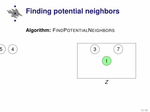
Finding potential neighbors

Algorithm: FINDPOTENTIALNEIGHBORS

Z

t

31745

13 / 45



Z

t

31745

13 / 45



Z

t

31745

13 / 45



Z

t

3

1

745

13 / 45



Z

t

3

1

745

Call OPTIMALNETWORK(Z ).

13 / 45



Z

t

3

7

145

13 / 45



Z

t

3

7

45

13 / 45



Z

t

3 745

13 / 45



Z

t

3 745

13 / 45



Z

t

3 7

8

The remaining nodes are potential neighbors oftarget node t .

13 / 45

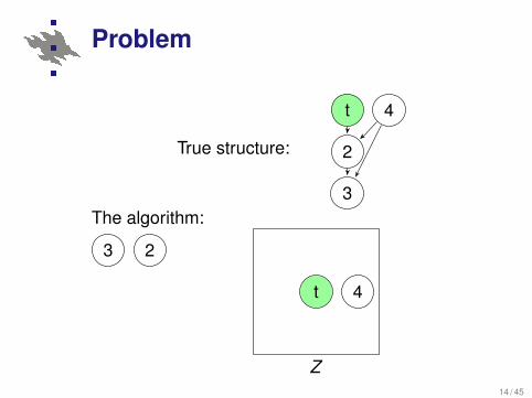
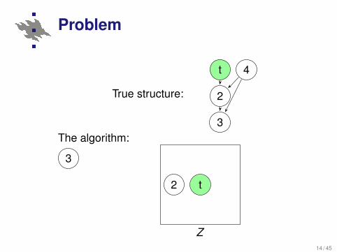
Problem

True structure:

t 4

2

3The algorithm:

Z

t

423

14 / 45

Problem

True structure:

t 4

2

3The algorithm:

Z

t 4

23

14 / 45

Problem

True structure:

t 4

2

3The algorithm:

Z

t

23

14 / 45

Problem

True structure:

t 4

2

3The algorithm:

Z

t2

3

14 / 45

Problem

True structure:

t 4

2

3The algorithm:

Z

t

2

3

14 / 45

Problem

True structure:

t 4

2

3The algorithm:

Z

t2

3

14 / 45

Problem

True structure:

t 4

2

3The algorithm:

Z

t2 3

14 / 45

Problem

True structure:

t 4

2

3The algorithm:

Z

t

2 3

14 / 45

Problem

True structure:

t 4

2

3The algorithm:

Z

t2 3

14 / 45

Symmetry correction forneighbors

Algorithm: FINDNEIGHBORS

1. Find potential neighbors Ht of t2. Remove nodes v ∈ Ht which do not have t as a

potential neighbor.3. The nodes remaining in the end are the

neighbors of t .

Note: Equivalent to symmetry correction in GLL.

15 / 45

Performance

Experiments: returns good results in practise.

Theoretical guarantees?

16 / 45

Asymptotic correctness

Does FINDNEIGHBORS always return the correctset of neighbors under certain assumptions whenthe sample size tends to infinity?

Compare:the generalized local learning (GLL) framework(Aliferis et al., 2010)greedy equivalent search (GES) (Chickering,2002)

17 / 45

Asymptotic correctness

Does FINDNEIGHBORS always return the correctset of neighbors under certain assumptions whenthe sample size tends to infinity?

Compare:the generalized local learning (GLL) framework(Aliferis et al., 2010)greedy equivalent search (GES) (Chickering,2002)

We don’t know for sure, but can say something.

17 / 45

Assumptions

The data distribution is faithful to a Bayesiannetwork. (i.e. there exists a perfect map of thedata distribution)

OPTIMALNETWORK uses a locally consistentand score equivalent scoring criterion (e.g.BDeu)

18 / 45

Network structure properties

DefinitionA structure A contains a distribution p if p can bedescribed using a Bayesian network with structureA (local Markov condition holds).

19 / 45


DefinitionA structure A contains a distribution p if p can bedescribed using a Bayesian network with structureA (local Markov condition holds).

DefinitionA distribution p is faithful to a structure A if allconditional independencies in p are implied by A.

19 / 45


DefinitionA structure A is a perfect map of p if

A contains p andp is faithful to A

20 / 45


DefinitionA structure A is a perfect map of p if

A contains p andp is faithful to A

⇒ no missing or extra independencies

Note: The property of having a perfect map is notclosed under marginalization.

20 / 45

Equivalent structures

DefinitionTwo structures are Markov equivalent if theycontain the same set of distributions.

A scoring criterion is score equivalent if equivalentDAGs always have the same score. (e.g. BDeu)

21 / 45

Equivalent structures

DefinitionTwo structures are Markov equivalent if theycontain the same set of distributions.

A scoring criterion is score equivalent if equivalentDAGs always have the same score. (e.g. BDeu)

⇒ learning possible up to an equivalence class

21 / 45

Consistent scoring criterion

Definition (Chickering, 2002)Let A′ be the DAG that results from adding the arcuv to A. A scoring criterion f is locally consistentif in the limit as data size grows, for all A, u and vhold:

If u 6⊥⊥p v |Av , then f (A′,D) > f (A,D).If u ⊥⊥p v |Av , then f (A′,D) < f (A,D).

⇒ relevant arcs increase score, irrelevant decrease

22 / 45

Finding neighbors: theory

In the limit of large sample size, we get thefollowing result:

LemmaFINDPOTENTIALNEIGHBORS returns a set thatincludes all true neighbors of target node t.

ConjectureFINDNEIGHBORS returns exactly the true neighborsof target node t.

23 / 45

Finding neighbors: Proof of thelemmaIn the limit of large sample size:

LemmaFINDPOTENTIALNEIGHBORS returns a set thatincludes all true neighbors of target node t.

Proof:assume v a neighbor of t in Afaithfulness ⇒ t and v not independent givenany subset of nodeslocal consistency ⇒ OPTIMALNETWORK on Zincluding t and v always returns a structurewith arc between t and vthus v kept in Z once added

24 / 45




25 / 45

Finding potential spouses

Algorithm: FINDPOTENTIALSPOUSES

Z

t

3 7

8

14526

26 / 45



Z

t

3 7

81

4526

26 / 45



Z

t

3 7

81

4

526

Call OPTIMALNETWORK(Z ).

26 / 45



Z

t

3

7

8

1

4

526

26 / 45



Z

t

3

7

8

1

526

26 / 45



Z

t

3 7

81

526

26 / 45



Z

t

3 7

81

6

The remaining new nodes are potential spouses oftarget node t .

26 / 45

Symmetry correction forspouses

Algorithm: FINDSPOUSES

1. Find potential spouses St of t .2. Add nodes which do have t as a potential

spouses.3. The nodes gathered in the end are the

spouses of t .

Note: Equivalent to symmetry correction in GLL.

27 / 45

Finding spouses: theory

Again, in the limit of large sample size:

LemmaFINDPOTENTIALSPOUSES returns a set thatcontains only true spouses of target node t.

ConjectureFINDSPOUSES returns exactly the true spouses oftarget node t.

28 / 45

Finding Markov blanket: theory

Summarising previous lemmas and conjectures:

ConjectureIf the data is faithful to a Bayesian network and oneuses a locally consistent and score equivalentscoring criterion then in the limit of large samplesize SLL always returns the correct Markov blanket.

29 / 45

Time and space requirements

OPTIMALNETWORK(Z ) dominates:O(|Z |22|Z |) timeO(|Z |2|Z |) space

Worst case: |Z | = O(n)⇒ total time at most O(n42n)

In practise: Networks are relatively sparse.⇒ significantly lower running times

30 / 45

SLL implementation

A C++ implementation.

OPTIMALNETWORK(Z ) procedure:dynamic programming algorithmBDeu scorefallback to GES for |Z | > 20

The implementation available athttp://www.cs.helsinki.fi/u/tzniinim/uai2012/

31 / 45

Experiments

Generated data from different Bayesiannetworks. (ALARM5 = 185 nodes, CHILD10 =200 nodes)

Compared score-based SLL toconstraint-based HITON by Aliferis et al.(2003, 2010).

Measured SLHD: Sum of Local HammingDistances between the returned neighbors(Markov blankets) and the true neighbors(Markov blankets).

32 / 45

Experimental results: neighbors

500 1000 5000100

200

300

400

Alarm5

500 1000 50000

100

200

300

400

Child10

HITON

SLL

Average SLHD for neighbors.

33 / 45

Experimental results: Markovblankets

500 1000 5000200

300

400

500

600

Alarm5

500 1000 50000

500

1000

Child10

HITON

SLL

Average SLHD for Markov blankets.

34 / 45

Experimental results: timeconsumption

500 1000 500010

100

1000

Alarm5

500 1000 500010

100

1000

Child10

SLL

HITON

Average running times (s).

35 / 45

Outline

Introduction

Local learning


Summary

36 / 45


Idea: Construct the global network structure basedon local results.

Implemented two algorithms:Constraint-based: SLL+CScore-based: SLL+G

Compared to:max-min hill-climbing (MMHC) by Tsamardinoset al. (2006)greedy search (GS)greedy equivalence search (GES) byChickering (2002)

37 / 45

SLL+C algorithm

Algorithm: SLL+C(constraint-based local-to-global)

1. Run SLL for all nodes.2. Based on the neighbor sets construct the

skeleton of the DAG.3. Direct the edges consistently (if possible) with

the v-structures learned during thespouse-phase of SLL. (see Pearl, 2000)

38 / 45

SLL+G algorithm

Algorithm: SLL+G(greedy search based local-to-global)

1. Run the first phase of the local neighborsearch of SLL for all nodes.

2. Construct the DAG by greedy search but allowadding arc between two nodes only if both areeach others potential neighbors.

⇒ Similar to MMHC algorithm.

39 / 45

Experimental results: SHD

500 1000 50000

100

200

300

Alarm5

500 1000 50000

100

200

300

Child10

GS

GES

MMHC

SLL+G

SLL+C

Average SHD.

40 / 45

Experimental results: scores

500 1000 50000.95

1

1.05

Alarm5

500 1000 50000.98

0.99

1

1.01

1.02

Child10

GS

GES

MMHC

SLL+G

SLL+C

Average normalized score.(1 = true network, lower = better)

41 / 45

Experimental results: timeconsumption

500 1000 500010

100

1000

Alarm5

500 1000 50001

10

100

1000

10000

Child10

GS

GES

MMHC

SLL+G

SLL+C

Average running times (s).

42 / 45

Outline

Introduction

Local learning


Summary

43 / 45

Summary

Score-based local learning algorithm: SLLConjecture: same theoretical guarantees asGES and constraint-based local learningExperiments: competitive alternative toconstraint-based local learning

Score-based local-to-global algorithmsExperiments: mixed results

Future directionsProve the guarantees (or lack thereof)Speed improvements

44 / 45

References

Constantin F. Aliferis, Alexander Statnikov, Ioannis Tsamardinos,Subramani Mani, and Xenofon D. Koutsoukos. Local causal andMarkov blanket induction for causal discovery and feature selection forclassification part I: Algorithms and empirical evaluation. Journal ofMachine Learning Research, 11:171–234, 2010.

Constantin F. Aliferis, Alexander Statnikov, Ioannis Tsamardinos,Subramani Mani, and Xenofon D. Koutsoukos. Local causal andMarkov blanket induction for causal discovery and feature selection forclassification part II: Analysis and extensions. Journal of MachineLearning Research, 11:235–284, 2010.

David Maxwell Chickering. Optimal structure identification with greedysearch. Journal of Machine Learning Reseach, 3:507–554, 2002.

Judea Pearl. Causality: Models, Reasoning, and Inference.Cambridge university Press, 2000.

Ioannis Tsamardinos, Laura E. Brown, and Constantin F. Aliferis. Themax-min hill-climbing Bayesian network structure learning algorithm.Machine Learning, 65:31–78, 2006.

45 / 45

Documents

Local Structure Discovery in Bayesian Networks · Local Structure Discovery in Bayesian Networks ... LGL framework (Tsamardinos et al., ... Local Structure Discovery in Bayesian Networks