A Bayesian multiple comparison approach for gene ... · Journal of Data Science 14(2016), 491-508 A Bayesian multiple comparison approach for gene expression data analysis Erlandson

Journal of Data Science 14(2016), 491-508

A Bayesian multiple comparison approach for gene expression data analysis

Erlandson F. Saraiva1∗, Lu´ıs A. Milan2

1Institute of Mathematics, Federal University of Mato Grosso do Sul

2Department of Statistcs, Federal University of Sao Carlos

Abstract: Methods used to detect differentially expressed genes in situations with

one control and one treatment are t-tests. These methods do not per- form well when

control and treatment variances are different. In situations with a control and more

than one treatment, it is common to apply analysis of variance followed by a Tukey

and/or Duncan test to identify which treatment caused the difference. We propose

a Bayesian approach for multiple comparison analysis which is very useful in the

context of DNA microarray experiments. It uses a priori Dirichlet process and Polya

urn scheme. It is a unified procedure (for cases with one or more treatments) which

detects differentially expressed genes and identify treatments causing the difference.

We use simulations to verify the performance of the proposed method and compare

it with usual methods. In cases with control and one treatment and control and more

than one treatment followed by Tukey and Duncan tests, the method presents better

performance when variances are different. The method is applied to two real data

sets. In these cases, genes not detected by usual methods are identified by the

proposed method.

Key words: Gene Expression, Bayesian approach, Prior Dirichlet process,

Polya urn, Multiple comparison.

1. Introduction

A common interest in gene expression data analysis is to identify genes with different

expression levels. Identifying these genes allows us to detect relationships between genes and

between genes and proteins; also, it allows us to identify which genes are involved in the origin

and/or evolution of diseases with genetic origin, or which genes react to a drug stimulus (Schena

et al., 1995; Allison et al., 2006; DeRisi et al., 1997; Arfin et al., 2000; Lonnstedt and Speed,

2001; Rosenfeld, 2007; Wu, 2001).

Gene expression data can be analyzed in at least three levels of increasing complexity (Baldi

and Long, 2001). In the first level, each gene is analyzed separately and the purpose is to verify

whether the expression levels are different in treatment and control conditions. In the second

492 A Bayesian multiple comparison approach for gene expression data analysis

level, clusters of genes are analyzed in terms of common functionalities and interactions. In the

third level, the purpose is to understand the relationship between genes and proteins.

Here we focus on identifying differentially expressed genes. One of the first proposed

approaches was the fold-change (Schena et al., 1995; Allison et al., 2006), where a gene is

considered differentially expressed if the average of the logarithm of the observed expression

levels in treatment and control differ by more than a cutoff value, Rc, which is previously

prefixed.

Another method used for gene expression data analysis is the two-sample t- test (T T ), see

Baldi and Long (2001) and Hatfield et al. (2003). A limitation for applying T T to gene

expression data is the usual small sample size, which may lead to underestimated variances and

low power of test. To avoid such limitations, some T T modifications were proposed, such as the

Cyber-t (CT) proposed by Baldi and Long (2001) and the Bayesian t-test (BTT) proposed by

Fox and Dimmic (2006). Basically, these methods modify the standard error estimate of the two

sample differences found in the denominator of the standard t statistic.

These methods can be applied to only two experimental conditions (control and treatment).

This is a drawback since in many microarray experiments, the gene expression response is

monitored under M , M > 2, treatment conditions.

The interest is to consider all M (M − 1)/2 pairwise treatments, (Dudoit et al.,

2003).

We propose a hierarchical Bayesian approach with a priori Dirichlet process, which compares

two or more experimental conditions. The comparison is made using the a posteriori probabilities

for models in a model selection procedure. The a posteriori probabilities are calculated using the

Polya urn scheme (Blackwell and MacQueen, 1973).

In order to verify the performance of the proposed method (denoted by PU ), we carried out

a simulation study with small sample sizes, which is usual in gene expression data analysis.

In situations with a control and a treatment, we compared the performance of PU with T T , CT

and BT T . We also considered situations with a control and two and three treatments. In these

cases, we compared the performance of PU with analysis of variance (ANOVA) followed

by the Tukey-test (Cox and Reid, 2000) and Duncan-test (Duncan, 1955). ANOVA was applied

to identify differentially expressed genes. As it does not discrimi- nate which treatments differ

from one another, we applied the Tukey-test and Duncan-test as a post hoc test.

The comparison among the methods was made in terms of the true positive rate and the false

discovery rate. The simulation study showed a better performance for PU , i.e., the greater true

positive rate and the smaller false discovery rate, for cases with different mean and variance. We

also applied these methods to two real data sets. The first is from an experiment with

Escherichia coli bacterium with a control and a treatment condition (Arfin et al., 2000). The

second refers to Plasmodium falciparum protein microarray with a control and two treatments,

obtained from the website cybert.ics.uci.edu (Baldi and Long, 2001).

This paper is structured using the hierarchical Bayesian model for the gene expression data

analysis, described in Section 2. The a posteriori probabilities are calculated using the Polya

urn scheme and the Bayes factor in Section 3. In Section 4, we compare the performance of the

Erlandson F. Saraiva, Lu´ıs A. Milan 493

proposed approach and methods usually considered. Section 5 concludes the paper with final

remarks.

2. Bayesian Model

Consider an experiment with N genes under experimental conditions E1, . . . , EM and E1 as

the control. For each gene g, g = 1, . . . , N , let {y1m, . . . , ynmm}be the set of measurements of

log-expression levels in experimental condition m, where nm is the sample size, for m = 1, . . . ,

M . Although this is not necessary for the proposed approach, to simplify notation we assume

a balanced design common to all genes so that nm = n, for m = 1, . . . , M .

Let Y = {Y1, . . . , YM} be the set of all observed expression levels for gene g, where Ym =

(y1m, . . . , ynm) ́ is a n × 1 vector of conditionally independent observations for treatment m.

Assume Yim ∼ F (θm), where F (θm) is a parametric distribution indexed by unknown parameters

θm. Denote the parametric space by Θ = {θ = (θ1, . . . , θM ); θm ∈ Rd, where d is the dimension

of θm, m = 1, . . . , M }.

Our interest is to verify whether a gene g is differentially expressed in different experimental

conditions, i.e., we search for a model which best fits the data and meets these conditions. These

models can be described as M0 : Θ0 = {θ; θ1 = . . . = θM}); M1 : Θ1 = {θ; θ1 ≠ θ2, θ2 = θ3

= . . . = θM}, or M2 : Θ2 = {θ; θ1 = θ2, θ2 ≠ θ3, = θ3 = . . . = θM}, and successively for all

combinations until MT : ΘT = {θ; θ1 ≠ . . . ≠ θM}.

The equality (or not) of θm’s determines partitions in parameter space Θ, i.e., Θ0, Θ1, . . . , ΘT

are disjointed and Θ0 ∪ Θ1 ∪ . . . ∪ ΘT = Θ. This allows us to develop a hierarchical Bayesian

approach using an a priori Dirichlet process (DP ) on θ1, . . . , θM in order to make simultaneous

comparisons of θm’s (Gopalan and Berry, 1998; Neal, 2000). This exploits the discreteness of the

Dirichlet process that allows parameters to be coincident with positive probability.

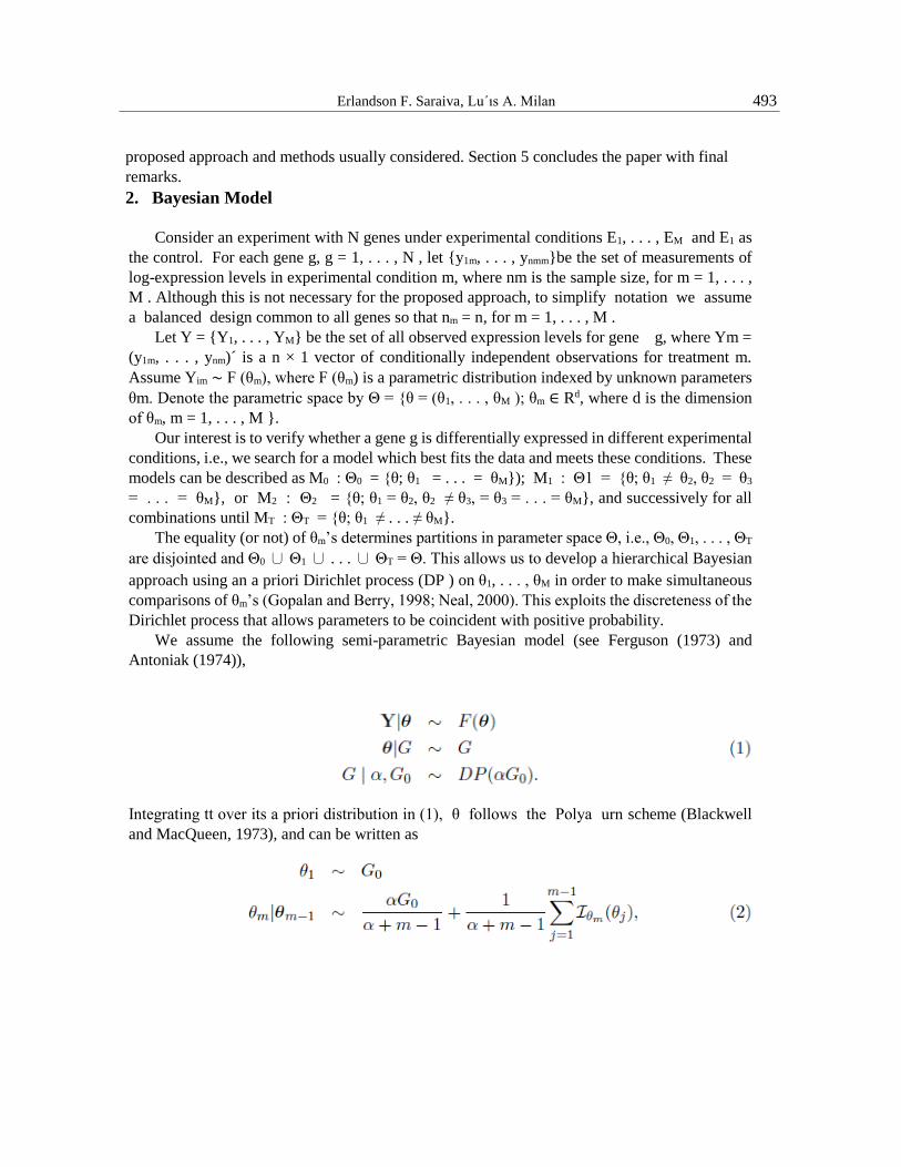
We assume the following semi-parametric Bayesian model (see Ferguson (1973) and

Antoniak (1974)),

Integrating tt over its a priori distribution in (1), θ follows the Polya urn scheme (Blackwell

and MacQueen, 1973), and can be written as


where θm−1 = (θ1, . . . , θm−1), Iθm (θj ) = 1 if θm = θj and Iθm (θj ) = 0 otherwise, for j ∈ {1, . . . , m

− 1} and m ∈ {2, . . . , M }.

Note that at each step of the sampling procedure defined in (2), θm replicates one of the previous

θ j 's, with probability1

𝑎+𝑚−1∑ 𝐼𝜃𝑚(𝜃𝑗)𝑚−1

𝑗=1 , or it assumes a new value, generated from the base

distribution G0, with probability 1

𝑎+𝑚−1 Thus, a sample from the joint distribution of θ1, . . . , θM

yields k groups (1 ≦ k ≦ M) of θm's with distinct values, ∅ 1, . . . ,∅ k, generated from the base

distribution G0.

2.1 A priori Dirichlet process via latent variables

Consider the latent variables c = (c1, . . . , cM ) in a way that cm = j indicates that θm =

φj , φj ∼ G0 for m = 1, . . . , M and j = 1, . . . , k. c classifies the observed data y =

(y1, . . . , yM ) in k groups, {D1, . . . , Dk}, where Dj = {ym; cm = j} with ⋃ 𝐷𝑗 = 𝑦𝑘𝑗=1 .

The likelihood function for c is

L(c|y) =∏ 𝑃 (𝐷𝑗 )𝑘𝑗=1 (3)

and πG0 (·) is the density of the base distribution G0.

Letting nj be the number of observations in Dj given the configuration cm−1 = (c1, . . . ,

cm−1), the Polya urn scheme in (2) can be described by

3. Multiple comparison


Updating the a priori probabilities in (5) and (6) via the likelihood function in (3), we

obtain the conditional a posteriori probabilities

where b is the normalizing constant and P (·) is given by (4).

In order to specify the mass parameter α, from (5) and (6), we define

See Gopalan and Berry (1998). Setting P (M0)/P (MT ) = 1, we obtain

3.1 Particular cases

Now we show some particular cases of (7) and (8).

3.1.1 Control and one treatment

In this case, we have M = 2, y = (y1, y2) and α = 1. Initialize with c1 = 1 and D1 =

{y1}.

Thus, from (7) and (8), we have


Let B21 = 𝑃(𝐷1)𝑃(𝑦2)

𝑃(𝐷1∪𝑦2) be the Bayes factor (Kass and Raftery, 1995). Compare models with

the first assuming Y1 ∼ F (φ1) and Y2 ∼ F (φ2), for φ1 ≠φ2, and the second assuming Y1, Y2 ∼

F (φ1). Thus

P (c2 = 1|c1 = 1, y) =1

1+𝛼𝐵21 and P (c = 2|c = 1, y) =

𝛼𝐵21

1+𝛼𝐵21

If P (c2 = 2|c1 = 1, y) > P (c2 = 1|c1 = 1, y) do c2 = 2. In this case, there is evidence for a

difference between the control and the treatment. Otherwise, do c2 = c1 = 1 considering that there

is not enough evidence for the difference.

3.1.2 Control and two treatment

We now have M = 3, y = (y1, y2, y3) and α = √2. Apply the procedure in 3.1.1 to classify

treatment 1 and define c2, then do the following procedure.

(i)If c2 = c1 = 1, i.e., treatment 1 does not differ in relation to the control,do D1 = {y1, y2}.

The a posteriori probabilities for c3 are given by

P (c3 = j | c2, y) = {

2

2+𝛼𝐵31 , 𝑓𝑜𝑟 𝑗 = 1

𝛼𝐵31

2+𝛼𝐵31 , 𝑓𝑜𝑟 𝑗 = 2

and B31 = 𝑃(𝐷1)𝑃(𝑦3)

𝑃(𝐷1∪𝑦3) , where c2 = (c1 = 1,c2 = 1).

If P(c3 = 2 | c2 , y) > P(c3 = 1 | c2 , y) do c3 = 2 , otherwise do c3 =1.

(ii) If c2 ≠ c1 (c1 = 1 and c2 = 2) then D1 = {y1} and D2 = {y2}.

The a posteriori probabilities for c3 are

Do c3 = (P (c3 = j| ·))𝑗=1,2,3argmax

.

In Appendix 1 of the additional matter (AM), we present a posteriori probabilities for the

case with a control and three treatments.

3.1.3 Algorithm for the general case

The proposed method can be expressed as:

(i) Initialize with c1 = 1, D1 = {y1}, k = 1 and fix α according to (9);

(ii) For m = 2, . . . , M do

(a) Calculate P (Dj ), P (Dj ∪ ym) and P (ym) according to (4), for j =

1, . . . , k;


(b) Calculate P(cm = j|cm-1 , y) ∝ 𝑛𝑗

𝛼+𝑚−1

𝑃(𝐷𝑗∪𝑦𝑚)

𝑃(𝐷𝑗) , as in (7); P(cm = k+1|cm-1 ,

y) ∝ 𝑛𝑗

𝛼+𝑚−1 𝑃(𝑌𝑚) , as in (8);

(c) If P(cm = j| ‧) = max𝑗=1,..,𝑘

(P(cm = 𝑗|‧) , P(cm = k+1| ‧) ), for j ∈

{1,…k }, do Dj = Dj ∪ ym and nj +1 . Else do Dk+1 = {ym} , nk+1 = 1 and k =

k+1;

Given the configuration c = (c1 . . . , cM ), if cm = 1 for all m = 1, . . . , M , we select

model M0, otherwise, if at least one cm ≠ 1, we select another model.Choosing M0 means no

differentially expressed gene for all treatments while in any other model it would imply at least

one treatment with a differentially expressed gene.

4. Data Analysis

We observed the performance of PU and compared it with standard methods using the

simulation.

Gene expression levels in control and treatments are generated from normal distribution,

Yim|µm, σ2 ∼ N (µm, σ2 ), for i = 1, . . . , n and m = 1, . . . , M .The normal assumption for

expression data (log-transformed) is usual in gene expression data analysis, see for example Baldi

and Long (2001); Hatfield et al.(2003); Fox and Dimmic (2006); Saraiva and Milan (2012);

Louzada et al. (2014).

Assume that

for m = 1, . . . , M , where µ0, λ, τ and β are known hyperparameters and IG(·) is the inverse

gamma distribution with mean β/(τ − 2), see Escobar and West (1995) and Casella et al., (2000).

Thus, from (4)


Consider (a, b) as roughly the interval which would include all observations produced by the

experiment. We defined the a priori distributions choosing τ and β such that E[𝜎𝑚2 ] =

𝛽

𝜏−2= R ,

where R is range of the interval R = b-a.Thus , we obtain β=(τ-2) ‧R and we set τ =3. The

hyperparameter µ0 was chosen to be the middle point of the interval µ0 = (a+b) /2 .We also set

λ=0.01.

4.1 Control and one treatment

For this case, we compared the performance of PU with T T , CT (Baldi and Long, 2001) and

the BT T (Fox and Dimmic, 2006).

4.1.1 Simulated data sets

We used µ1 = −14 and σ12 = 0.8 to simulate the data sets.These values are the mean and

variance of the expression levels (log transformed) from the control group of the Escherichia coli

bacterium data set. The sample sizes used are 4 and 8.

To verify how the method performs when treatment parameters θ2 = (µ2, σ22) move away

from the control parameters θ1 = (µ1, σ12), we simulate this using µ2 = µ1 ± δσ1 and σ2 = γσ1,

for δ ∈ {0.0, 0.5, 1.0, 1.5, 2, 2.5, 3} and γ ∈ {1, 2, 3}.

Data sets were generated to mimic a mix of both differentially and non- differentially

expressed genes where the proportion of differentially expressed genes is small. We fixed the

proportion of differentially expressed genes at 5%, being 3% and 2% for situations over and

under expressed, respectively.

The data sets were simulated following the steps. For g = 1, . . . , N , N = 1000, simulate ug

∼ U (0, 1):

(i) If ug ≤ 0.95 fix µ2 = µ1 and σ2 = σ1. Let the index variable IIg = 0 to indicate

that case g is generated under M0;

(ii) If 0 .95 < ug ≤ 0.98 fix µ2 = µ1 + δσ1 and σ2 = γσ1. Set IIg = 1 to indicate that

case g is generated under M1;

(iii) If ug > 0.98 fix µ2 = µ1 − δσ1 and σ2 = γσ1. Set IIg = 1 to indicate that case g is

generated under M1;

(iv) Simulate Yim ∼ N (µm, σm2 ), for m = 1, 2 and i = 1, . . . , n.

After generating the data sets, we apply PU and t-tests to identify the cases with a difference.

To record cases identified with a difference by PU , we consider an index variable IP U = 1 if P

(c2 = 2|c1 = 1, y) > 0.5 and IP U = 0 otherwise.Similarly, for T T , CT and BT T , we consider

Imethod = 1 (where the method is TT or CT or BTT ) for cases with p − value < 0.05 and IIgmethod

= 0 otherwise.

We define as performance indicators the true positive rate, TPr, and the false discovery rate,

FDr, as


When δ = 0 and γ = 1 no case is generated under the alternative model, for this case T Prmethod

= 0.

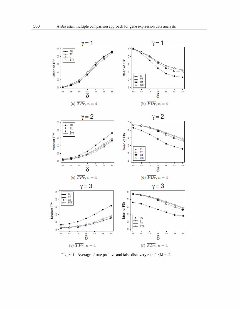
We generate L = 100 different artificial data sets for each pair (δ, γ), as described above.

The average values of TPr and FDr, denoted by 𝑇𝑃𝑟method

and 𝐹𝐷𝑟method

, for n = 4, are

presented in Figure 1. Figure 1 in Appendix 2 of the additional matter (AM) shows the 𝑇𝑃𝑟

and 𝐹𝐷𝑟 for n = 8.

Average true positive curves are presented in Figure 1-a,c,e. As can be observed in Figure

1-a, the performance is similar for n = 4 and all values of δ. For

sample size n = 8 (Figure 1-a of AM), equal variance, γ = 1, and small changes in mean (0.5

≤ δ ≤ 2.0), T T , CT and BT T show a better performance than PU, while for δ ≥ 2.5 all methods

are similar.

As the difference in variance increases, γ = 2 and γ = 3, PU performs better than all methods

tested, and the performance improves as the difference increases, as can be observed in Figures

1-c and 1-e.

Figure 1-b,d,f shows the average false positive (also see Figure 1-b,d,f of the AM).

Considering the condition of equal variances, Figure 1-b, all methods are similar for equal means

and as the difference between the means increases, the performance of PU improves more rapidly

than in the other methods. For different variances, Figures 1-d and 1-f, PU is better in all tested

situations. This good performance of PU for small differences in means and large differences in

variance is especially interesting for detecting differentially expressed genes.


Figure 1: Average of true positive and false discovery rate for M = 2.


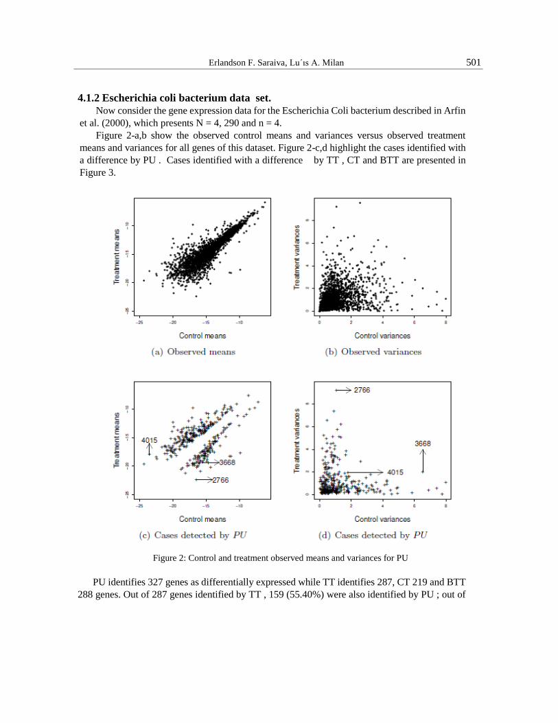
4.1.2 Escherichia coli bacterium data set.

Now consider the gene expression data for the Escherichia Coli bacterium described in Arfin

et al. (2000), which presents N = 4, 290 and n = 4.

Figure 2-a,b show the observed control means and variances versus observed treatment

means and variances for all genes of this dataset. Figure 2-c,d highlight the cases identified with

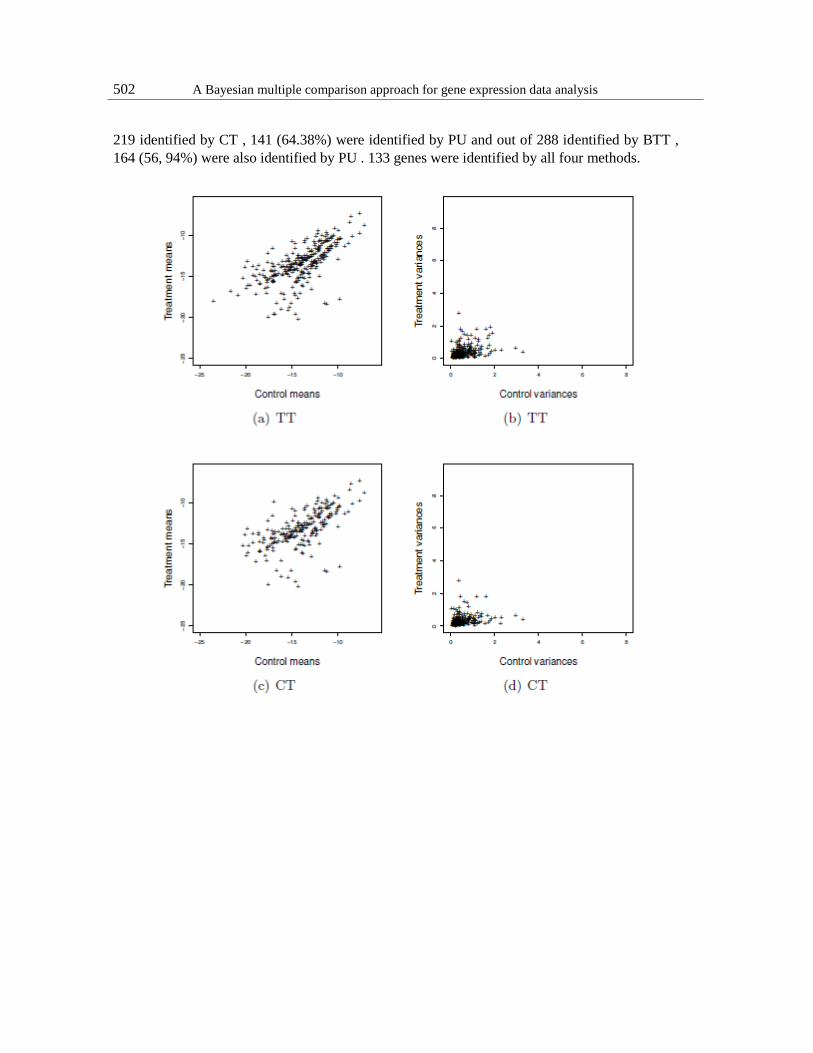
a difference by PU . Cases identified with a difference by TT , CT and BTT are presented in

Figure 3.

Figure 2: Control and treatment observed means and variances for PU

PU identifies 327 genes as differentially expressed while TT identifies 287, CT 219 and BTT

288 genes. Out of 287 genes identified by TT , 159 (55.40%) were also identified by PU ; out of


219 identified by CT , 141 (64.38%) were identified by PU and out of 288 identified by BTT ,

164 (56, 94%) were also identified by PU . 133 genes were identified by all four methods.


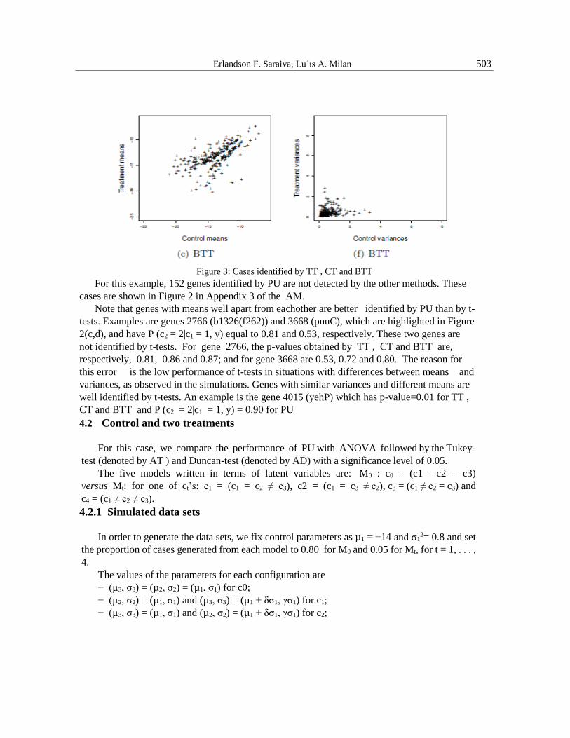
Figure 3: Cases identified by TT , CT and BTT

For this example, 152 genes identified by PU are not detected by the other methods. These

cases are shown in Figure 2 in Appendix 3 of the AM.

Note that genes with means well apart from eachother are better identified by PU than by t-

tests. Examples are genes 2766 (b1326(f262)) and 3668 (pnuC), which are highlighted in Figure

2(c,d), and have P (c2 = 2|c1 = 1, y) equal to 0.81 and 0.53, respectively. These two genes are

not identified by t-tests. For gene 2766, the p-values obtained by TT , CT and BTT are,

respectively, 0.81, 0.86 and 0.87; and for gene 3668 are 0.53, 0.72 and 0.80. The reason for

this error is the low performance of t-tests in situations with differences between means and

variances, as observed in the simulations. Genes with similar variances and different means are

well identified by t-tests. An example is the gene 4015 (yehP) which has p-value=0.01 for TT ,

CT and BTT and P (c2 = 2|c1 = 1, y) = 0.90 for PU

4.2 Control and two treatments

For this case, we compare the performance of PU with ANOVA followed by the Tukey-

test (denoted by AT ) and Duncan-test (denoted by AD) with a significance level of 0.05.

The five models written in terms of latent variables are: M0 : c0 = (c1 = c2 = c3)

versus Mt: for one of ct’s: c1 = (c1 = c2 ≠ c3), c2 = (c1 = c3 ≠ c2), c3 = (c1 ≠ c2 = c3) and

c4 = (c1 ≠ c2 ≠ c3).

4.2.1 Simulated data sets

In order to generate the data sets, we fix control parameters as µ1 = −14 and σ12= 0.8 and set

the proportion of cases generated from each model to 0.80 for M0 and 0.05 for Mt, for t = 1, . . . ,

4.

The values of the parameters for each configuration are

− (µ3, σ3) = (µ2, σ2) = (µ1, σ1) for c0;

− (µ2, σ2) = (µ1, σ1) and (µ3, σ3) = (µ1 + δσ1, γσ1) for c1;

− (µ3, σ3) = (µ1, σ1) and (µ2, σ2) = (µ1 + δσ1, γσ1) for c2;


− (µ2, σ2) = (µ1 + δσ1, γσ1) and (µ3, σ3) = (µ2, σ2) for c3;

− (µ2, σ2) = (µ1 + δσ1, γσ1) and (µ3, σ3) = (µ2 + δσ2, γσ2) for c4,

for δ ∈ {0, 0.50, 1, 1.50, 2, 2.50, 3, 3.50, 4} and γ ∈ {1, 2, 3}.

The generation of a simulated data set is as follows. For g = 1, . . . , N , generate ug from

U ∼ U (0, 1);

(i) If ug ≤ 0.80, fix parameters values according to c0. Let the index vector

Gg = (1, 1, 1) to indicate that case g is generated from M0;

(ii) If 0 .80 < ug ≤ 0.85, fix parameters values according to c1 and set Gg = (1, 1, 2);

(iii) If 0 .85 < ug ≤ 0.90, fix parameters values according to c2 and set Gg = (1, 2, 1);

(iv) If 0 .90 < ug ≤ 0.95, fix parameters values according to c3 and set Gg = (1, 2, 2);

(v) If ug > 0.95, fix parameters values according to c4 and set Gg = (1, 2, 3);

(vi)Generate Yim ∼ N (µm, σm2 ), for m = 1, 2, 3 and i = 1, . . . , n.

For each pair (δ, γ), we generate L = 100 data sets according to steps (i) to (vi) described

above and the results are presented using 𝑇𝑃𝑟 and 𝐹𝐷𝑟, see Appendix 4 of AM.

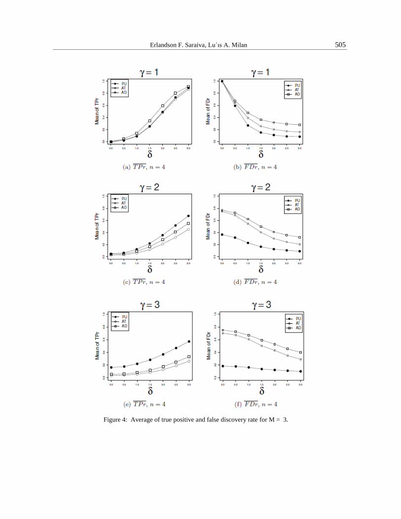
Figure 4-a,c,e shows the true positive rate, 𝑇𝑃𝑟. For equal variance, γ = 1, and n = 4, Figure

4-a, the performance of PU is similar to AT and slightly worse than AD. Increasing the

sample size, n = 8 (Figure 3-a in Appendix 5 of AM), AD is better than PU and AT . For

different variances, Figures 4-c and 4-e (Figures 3-c and 3-e in Appendix 5 of AM), PU is

better than both AT and AD.

The graphs in Figure 4-b,d,f (Figure 3-b,d,f in Appendix 5 of AM) show the false

discovery rate. In all tested situations, PU presented better results, especially in cases where the

variances are different, as shown in Figures 4-d and 4-f (Figures 3-d,f of AM), with the

performance increasing as the difference in variance increases and for a small difference in means.

Appendix 6 of AM shows a comparison of performance of the methods for

M = 4. For this case, the PU also presents higher 𝑇𝑃𝑟 and smaller 𝐹𝐷𝑟.

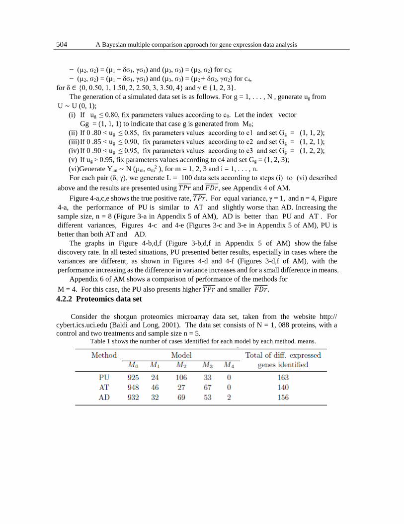
4.2.2 Proteomics data set

Consider the shotgun proteomics microarray data set, taken from the website http://

cybert.ics.uci.edu (Baldi and Long, 2001). The data set consists of N = 1, 088 proteins, with a

control and two treatments and sample size n = 5. Table 1 shows the number of cases identified for each model by each method. means.


Figure 4: Average of true positive and false discovery rate for M = 3.


Out of the 140 rejected null models by AT , 105 (75%) were also rejected by PU ; out of the

46 cases identified by AT as M1, 15 (32.61%) were also identified by PU ; all 27 cases identified

as M2 by AT , were also identified by PU ; and out of the 67 cases identified under M3 by AT ,

17 (25.37%) were also identified by PU .

Out of the 156 rejected null models by AD, 112 (71.79%) were also rejected by PU ; out of

the 32 cases identified by AD as M1, 15 (46.88%) were also identified by PU ; out of the 69

cases identified as M2 by AD, 49 (71.01%) were also identified by PU ; out of the 53 cases

identified as M3 by AD, 18 (33.96%) were also identified by PU ; and the two cases identified

as M4 by AD (proteins 60 and 649) were not identified by PU as M4, but as M1.

Tables 2 and 3 in Appendix 7 of AM show the ten most evident cases identified by PU and

AT -AD, respectively.

For this proteomics data, 51 null hypothesis rejected by PU were not rejected by any of the other

methods. These cases are shown in Table 4 in Appendix 8 of the AM.

5. Discussion

Results from simulations showed a better performance for PU than TT , CT and BTT , for

experiments with control and one treatment. This was clearer in situations with different

variances. For experiments with control and two or three treatments, we compared the

performance of PU with ANOVA followed by the Tukey-test (AT ) or Duncan-test (AD). Once

more, PU presented a better performance than AT and AD emphasizing itself in cases with

different variances. Methods were also applied to real data sets with control and one treatment

and control and two treatments. In both cases, PU showed a better performance. From a biological

point of view, the main interest is that PU brings to light genes that are not identified when

using the other methods considered in comparisons, (TT , AT and AD), AT or AD. This suggests

an eventual complementarity

of the methods.

Additional points in favour of PU are: (1) It is easier to use, especially when M > 2

and (2) it performs well in situations with small sample sizes which are common in gene

expression data analysis. Besides this, the PU can be easily implemented in usual software such

as the software R. The code used for computing is in the R language and can be obtained by e-

mail from the first author.

Acknowledgment

We thank the Editor and the referees for their comments, suggestions and criticisms which

have led to improvements of this article. The first author ac- knowledges the Brazilian institution

CNPq.


References

[1] Allison, D. B., Cui, X., Page, G. P. and Sabripour, M. (2006). Microarray data analysis: from

disarray to consolidation and consensus, Nat. Rev. Genet., 7, 55-65.

[2] Antoniak, C. E. (1974). Mixture of processes Dirichlet with applications to Bayesian

nonparametric problems. The Annals of Statistics, 2, 1152-1174.

[3] Arfin, S. M., Long, A. D., Ito, E. T., Tolleri, L., Riehle, M. M., Paegle, E. S., Hatfield, G.

W. (2000). Global gene expression profiling in Escherichia Coli K12. J. Biol. Chem, 275,

29672-29684.

[4] Baldi, P., Long, D. A. (2001). A Bayesian framework for the analysis of microarray

expression data: regularized t-test and statistical inferences of gene changes.

Bioinformatics, 17, 509-519.

[5] Blackwell, D. and MacQueen, J. B. (1973). Ferguson distribution via Polya urn schemes.

The Annals of Statistics, 1, 353-355.

[6] Casella, G., Robert, C., and Wells, M. (2000). Mixture models, latent variables and

partitioned importance sampling. Technical Report 2000-03, CREST, INSEE, Paris.

[7] Cox, D. R. and Reid, N. M. (2000). The theory of design of experiments.

Chapman-Hall/CRC.

[8] DeRisi, J.L., Iyer, V.R. and Brown, P.O. (1997). Exploring the metabolic and genetic control

of gene expression on a genomic scale. Science, 278, 680-68.

[9] Dudoit, S., Shaffer, J. P. and Boldrick, J. C. (2003). Multiple hypothesis testing in

microarray experiments. Statistical Science, 18(1), 71-103.

[10] Duncan, D B. (1955). Multiple range and multiple F tests. Biometrics, 11, 1-42.

[11] Escobar, M. D. and West, M. (1995). Bayesian Density Estimation and Inference using

Mixtures. Journal of the American Statistical Association, 90, 577– 588.

[12] Ferguson, S. T. (1973). A Bayesian analysis of some nonparametric problems.

The Annals of Statistics, 2, 209-230.

[13] Fox, R. J. and Dimmic, M. W. (2006). A two-sample Bayesian t-test for microarray data.

BMC Bioinformatics, 7:126.

[14] Gopalan, R.; Berry, D. A. (1998). Bayesian multiple comparisons using Dirich- let process

priors. Journal of the American Statistical Association, vol.93, No.443, 1130-1139.


[15] Hatifield, G. W., Hung, S. and Baldi, P. (2003). Differential analysis of DNA microarray

gene expression data. Molecular Microbiology, 47(4), 871-877.

[16] Kass, R., and Raftery, A. (1995). Bayes Factor. Journal of the American Statistical

Association, 90, 773-795.

[17] Lonnstedt, I. Speed, T. P. (2001). Replicated microarray data. Statistica Sinica,

12, 31-46.

[18] Louzada, F, Saraiva, E. F., Milan, L. A. and Cobre, J. (2014). A predictive Bayes factor

approach to identify genes differentially expressed: an application to Escherichia coli

bacterium data. Brazilian Journal of Probability Statistics., 28, 167-189.

[19] Neal, R. M. (2000). Markov chain sampling methods for Dirichlet process mixture models.

Journal of Computational and Graphical Statistics, 9, 249-265.

[20] Rosenfeld, S.(2007) Detection of Differentially Expressed Genes In Small Sets of cDNA

Microarrays. Journal of Data Science, 5, 00-00(JDS-341).

[21] Saraiva, E. F. and Milan, L. A. (2012). Clustering Gene Expression Data using a Posterior Split-

Merge-Birth Procedure. Scandinavian Journal of Statistics, 39, 399-415.

[22] Schena, M., Shalon, D., Davis, R. W. and Brown, P. O. (1995). Quantita- tive

monitoring of gene expression patterns with a complementary DNA microarray. Science,

270, 467-470.

[23] Wu, T. D. (2001). Analyzing gene expression data from DNA microarray to identify

candidates genes. Journal of Pathology, 195(1), 53-65.

Received June 25, 2014; accepted September 28, 2014

Erlandson F. Saraiva

Institute of Mathematics

Federal University of Mato Grosso do Sul Campo

Grande, MS, Brazil

Lu´ıs A. Milan Department of

Statistics

Federal University of Sao Carlos Sao

Carlos, SP, Brazil

Documents

A Bayesian multiple comparison approach for gene ... · Journal of Data Science 14(2016), 491-508 A Bayesian multiple comparison approach for gene expression data analysis Erlandson