Embed Size (px)
Citation preview

The Centre for Australian Weather and Climate Research
A partnership between the Bureau of Meteorology and CSIRO
A Bayesian methodology for detecting anomalous
propagation in radar reflectivity observations
Justin R. Peter, Alan Seed, Peter Steinle, Susan Rennie and Mark Curtis
CAWCR Technical Report No. 077
December 2014


A Bayesian methodology for detecting anomalous
propagation in radar reflectivity observations
Justin R. Peter, Alan Seed, Peter Steinle, Susan Rennie and Mark Curtis.
The Centre for Australian Weather and Climate Research
– a partnership between CSIRO and the Bureau of Meteorology
CAWCR Technical Report No. 077
December 2014 ISSN: 1835-9884 Authors: Peter, J.R., Seed, A., Steinle, P., Rennie, S. and Curtis, M. Title: A Bayesian methodology for detecting anomalous propagation in radar
reflectivity observations.
ISBN: 978-1-4863-0473-8 (Electronic Resource PDF) Series: CAWCR technical report. Notes: Includes bibliographical references and index.
Contact details
Enquiries should be addressed to:
Dr Justin R. Peter
Centre for Australian Weather and Climate Research
GPO Box 1289K
Melbourne
Vic 3001
Australia
Phone: +61 3 9669 4838

Copyright and disclaimer
© 2014 CSIRO and the Bureau of Meteorology. To the extent permitted by law, all rights are reserved
and no part of this publication covered by copyright may be reproduced or copied in any form or by
any means except with the written permission of CSIRO and the Bureau of Meteorology.
CSIRO and the Bureau of Meteorology advise that the information contained in this publication
comprises general statements based on scientific research. The reader is advised and needs to be
aware that such information may be incomplete or unable to be used in any specific situation. No
reliance or actions must therefore be made on that information without seeking prior expert
professional, scientific and technical advice. To the extent permitted by law, CSIRO and the Bureau
of Meteorology (including each of its employees and consultants) excludes all liability to any person
for any consequences, including but not limited to all losses, damages, costs, expenses and any other
compensation, arising directly or indirectly from using this publication (in part or in whole) and any
information or material contained in it.

A Bayesian methodology for detecting anomalous propagation in radar reflectivity observations i
Contents
1. Introduction ....................................................................................................... 1
1.1 On-site processing .................................................................................................... 2
1.2 Post-data-acquisition processing .............................................................................. 2
1.3 An example of spurious radar returns caused by anomalous propagation .............. 3
2. A brief climatology of anaprop in the Sydney region ..................................... 5
2.1 Atmospheric conditions required for anaprop ........................................................... 5
2.2 Datasets .................................................................................................................... 7
2.3 Prevalence of ducts .................................................................................................. 8
3. Radar data ....................................................................................................... 11
4. Bayes clutter classifier ................................................................................... 12
4.1 Feature fields input to the Bayes classifier ............................................................. 13 4.1.1 Texture of reflectivity ........................................................................................... 13 4.1.2 SPIN ................................................................................................................... 13 4.1.3 Vertical profile of reflectivity ................................................................................ 14
4.2 Construction of conditional PDFs from a training dataset ...................................... 14
4.3 Transformation of the conditional PDFs ................................................................. 21
4.4 Independence of the feature fields ......................................................................... 24
5. Results ............................................................................................................. 26
5.1 Varying input feature fields on the training dataset ................................................ 26
5.2 Verification of the classifier ..................................................................................... 28
5.3 Application to the training dataset precipitation cases ........................................... 29
5.4 Application to a case of rain embedded in anaprop ............................................... 30
5.5 The effect of the reflectivity threshold ..................................................................... 32
5.6 Application to radars other than Kurnell ................................................................. 33
5.7 A strength of classification index ............................................................................ 35
6. Summary and conclusions ............................................................................. 38
References ................................................................................................................ 40

ii A Bayesian methodology for detecting anomalous propagation in radar reflectivity observations
List of figures
Fig. 1: (Left) PPI obtained from the Kurnell radar at 1100 UTC (2200 LT). Some of the returns are of the order 35–45 dBZ which is also typical of values obtained from measurements of showers in this location. (Right) RHI obtained at an azimuth of 100 degrees from North. Significant reflectivity values are prevalent between 80 to 130 km range, however, they are only present in the lower two elevations, signifying their source is from anaprop. Only reflectivities above 10 dBZ are shown. The azimuth of the RHI is indicated by the black line shown on the PPI. ............................................... 4
Fig. 2: Schematic of the different propagation conditions of microwave radiation in the atmosphere. From US Weather Bureau (1967) ............................................................. 6
Fig. 3: (Left) sounding obtained at 0018 UTC (11.18 EDT) at Sydney airport. A strong temperature and humidity inversion is present at around 980 hPa. Despite being obtained 11 hours before the PPI shown in Fig. 1, the inversion and ducting layer persisted for many hours and was responsible the presence of anaprop. (Right) The corresponding profile of refractivity. The delineation of conditions for ducting, super refraction, normal refraction and sub refraction are indicated. Note the presence of many different refractivity conditions in the lowest 5 km. ............................................... 7
Fig. 4: Climatology of ducts, super refractive and sub refractive conditions at Sydney airport for the period 1 January 2004 to 31 December 2009. Only measurements below 850 hPa have been included in the calculation. .................................................................... 8
Fig. 5: PDFs of the frequency of occurrence of atmospheric refractivity conditions as a function of height. Ducts and super-refractive conditions display a greater propensity to form in the lowest ~ 30 hPa of the atmosphere, while sub-refractive conditions show a nearly linear relationship in the lowest 200 hPa of the atmosphere. .............................. 9
Fig. 6: Seasonal cycle of duct heights at Sydney. ............................................................... 10
Fig. 7: PPI radar reflectivity displays of the meteorological cases chosen for the training dataset. Clockwise from top left: squall line, widespread shallow stratiform rain, deep convection, widespread deep stratiform rain with embedded convection. ................... 16
Fig. 8: The texture feature field (TDBZ) corresponding to the images shown in Fig. 7. ...... 18
Fig. 9: The SPIN feature field corresponding to the images shown in Fig. 7. ..................... 19
Fig. 10: (Left) The TDBZ feature field and (Right) the SPIN feature field for the anaprop case presented in Fig. 1. .............................................................................................. 20
Fig. 11: Probability distribution functions of the feature fields, TDBZ, SPIN and VPDBZ. PDFs are shown for each of the meteorological situations and for anaprop. These PDFs represent the likelihood function in Bayes formula (Equation (4)). Note the logarithmic axes for TDBZ. ........................................................................................... 20
Fig. 12: The log-likelihood as a function of λ (see Equation (9)). The value of λ which maximizes the log-likelihood function provides the best value to transform the data to an approximately normal distribution via Equation (8)). The dotted lines represent the 95 per cent confidence interval for λ. This curve is the log-likelihood function evaluated for the TDBZ field of the anaprop case. Values for TDBZ and SPIN for each case are presented in Table 3. .................................................................................................... 22
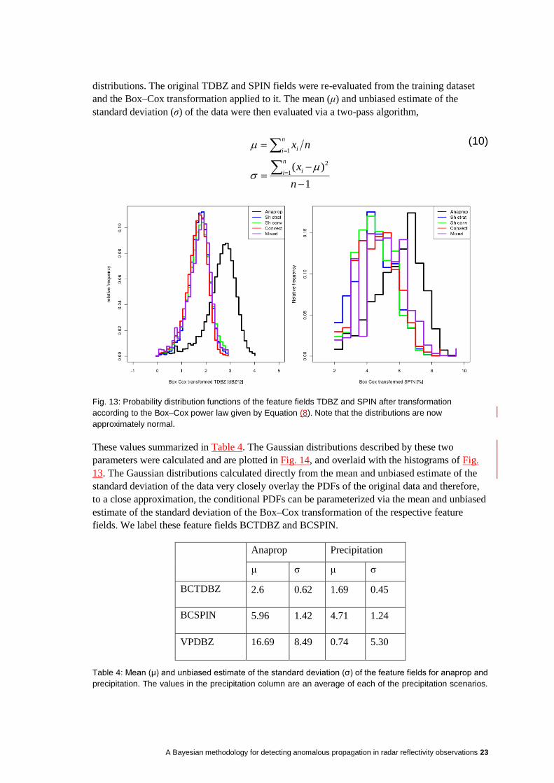
Fig. 13: Probability distribution functions of the feature fields TDBZ and SPIN after transformation according to the Box–Cox power law given by Equation (8). Note that the distributions are now approximately normal. .......................................................... 23
Fig. 14: Same as Fig. 13 including the best-fit normal curves determined from the mean and unbiased estimate of the standard deviation of the Box–Cox transformed training datasets. ....................................................................................................................... 24

A Bayesian methodology for detecting anomalous propagation in radar reflectivity observations iii
Fig. 15: Scatter plots of each of the Box–Cox transformed variables. Values for precipitation are shown in grey while anaprop values are in black. As for Fig. 14, the values for anaprop are separated from those for precipitation. .................................... 24
Fig. 16: The results of the naïve Bayes classifier (NBC) applied to the anaprop training dataset presented in Fig. 1. The image on the left was obtained using BCTDBZ only for classification, while the image on the right used BCTDBZ and VPDBZ. ................. 26
Fig. 17: Images transmitted for public display using the Bureau’s current clutter mitigation system. The images correspond to the anaprop data presented in Fig. 1 and the shallow stratiform case presented in Fig. 7. It can be seen that the current system is ineffective at removing anaprop, especially far from the radar, while it also removes many genuine precipitation pixels, especially close to the radar. ................................. 27
Fig. 18: The results of the NBC applied to the precipitation cases from the training dataset. The original reflectivity images are shown in Fig. 7. ..................................................... 30
Fig. 19: An example of anaprop and a convective storm obtained from the Kurnell radar on 22 January 2010. Anaprop is present in the northeast and a convective storm in the southeast. The top left panel is a PPI image obtained at the lowest elevation (0.7°), while the top right panel was obtained at the next highest elevation (1.5°). Note the absence of anaprop in the higher elevation. The bottom left panel is an RHI obtained at an azimuth of 40° through the anaprop, while the lower right panel is an RHI at 112° and shows the presence of a convective system extending to nearly 10 km height. The azimuths of the RHIs are indicated by the black line in the PPIs. ................................ 31
Fig. 20: The results of the NBC applied to Fig. 19 using BCTDBZ and VPDBZ as input feature fields. The NBC has classified the anaprop correctly, completely eliminating the returns in the northeast, however, some pixels which are returns from precipitation have been incorrectly classified as clutter. ................................................................... 32
Fig. 21: (left) PPI image of mixed anaprop and precipitation using a minimum reflectivity threshold of −30 dBZ. Note the increase in returns over land close to the radar compared to Fig. 19. These returns were most likely due to Bragg scattering. (right) Results of the NBC using −30 dBZ as the minimum reflectivity threshold. .................. 33
Fig. 22: An example of anaprop and shallow maritime cumulus convection observed from three separate radars: Terrey Hills, Kurnell and Wollongong) each with different operating characteristics. .............................................................................................. 34
Fig. 23: The NBC applied to the PPIs from Fig. 22 .............................................................. 34
Fig. 24: The ‘strength of classification’ index evaluated for each of the precipitation cases from the training dataset. A larger value indicates a larger confidence that a pixel is precipitation. .................................................................................................................. 36
Fig. 25: SOC index PDFs evaluated for each of the precipitation training datasets. Theoretically the SOC can have a maximum value of one; however, the majority of values are confined below 0.5. ..................................................................................... 37

iv A Bayesian methodology for detecting anomalous propagation in radar reflectivity observations
List of tables
Table 1: Operating parameters for the Kurnell radar. .......................................................... 11
Table 2: Summary of time periods, number of radar volumes and number of unique reflectivity samples used for the training dataset. ........................................................ 14
Table 3: Calculated values of λ for the Box–Cox transformation described by Equation (8) for anaprop and each of the precipitation cases. The last column shows the average value of λ for all precipitation cases combined. ............................................................ 22
Table 4: Mean (μ) and unbiased estimate of the standard deviation (σ) of the feature fields for anaprop and precipitation. The values in the precipitation column are an average of each of the precipitation scenarios. They were obtained by applying the Box–Cox transformation to the feature fields of the training data and then computing μ and σ of the transformed distribution. ......................................................................................... 23
Table 5: Pearson coefficient of correlation for anaprop conditions and the differing precipitation cases. All possible coefficients are shown for the original feature fields (TDBZ, SPIN and VPDBZ) and the Box–Cox transformed values (BCTDBZ, BCSPIN and VPDBZ). ................................................................................................................. 25
Table 6: Contingency table constructed from the anaprop and precipitation training datasets. A minimum reflectivity threshold of 10 dBZ was applied. ............................. 28

A Bayesian methodology for detecting anomalous propagation in radar reflectivity observations 1
1. INTRODUCTION
Radar data within the Bureau of Meteorology (the Bureau) are currently utilised in a
predominantly qualitative manner. Their main use is for nowcasting—predicting the weather
within a timescale of several hours and spatial scales of several kilometres. Forecasters
routinely use it to visually determine the presence (or lack thereof) of severe storms and guide
the issuance of severe weather or flash flood warnings. To enable quantitative use of radar data,
the Bureau initiated the Strategic Radar Enhancement Project (SREP). Specifically, radar data
can be assimilated in numerical weather prediction (NWP) models to improve their initial
conditions and subsequent predictions. Quality control (QC) of the radar data is central to
providing the data assimilation system with clean data and estimates of the error characteristics
of the observations. It will also benefit quantitative precipitation estimation and forecasting
(QPE and QPF) and generation of public weather radar images.
Weather radar is a microwave pulse and, like all electromagnetic radiation, its path is influenced
by the refractive index of the medium (in this case the atmosphere) through which it propagates.
The refractive index of the atmosphere is related to temperature, pressure and water vapour
content. In some instances, the vertical gradients of these variables can be large enough so as to
bend the radar beam from the path it would take in a standard atmosphere, a phenomenon
known as anomalous propagation (anaprop). Furthermore, if the gradients of temperature or
moisture are large enough the radar beam can become trapped in shallow layers in the
atmosphere (termed ducting) producing returns from the ground. Such conditions are frequently
encountered over the ocean, under the presence of a high pressure cell where significant
evaporation from the ocean coupled with a temperature inversion can produce suitable
conditions for ducting of the radar beam. Much of Australia’s population resides by the coast
and as a result, a large proportion of the Bureau of Meteorology’s (the Bureau) radar network is
also located there, resulting in the potential for a large proportion of radar data to be
contaminated by returns from anaprop of the radar beam.1
Anaprop has been observed since the advent of radar and the meteorological conditions which
produce it have been well described in the literature (e.g. Doviak and Zrnić, 1984; Meischner et
al., 1997). It is easily recognized by operational forecasters due to its shallow vertical extent and
transient temporal characteristics, however, these same properties make its automated detection
difficult. Automated detection of anaprop is of fundamental importance in quantitative weather
radar applications, such as data assimilation for numerical weather prediction (NWP), as
assimilation of anaprop could lead to large overestimates of precipitation totals and initiate
spurious convection. Furthermore, small errors in quantitative precipitation estimation (QPE)
1 The term anaprop is most often used to describe the returns visible on radar images under
conditions where ducting layers occur (an extreme example of anaprop), however it also refers
to departures from normal propagation which the radar beam may experience. We will generally
use anaprop in its former use when referring to its manifestation in radar images, however, in
some instances will use it to describe the refraction of the radar beam under non-standard
atmospheric conditions.

2 A Bayesian methodology for detecting anomalous propagation in radar reflectivity observations
have been shown to propagate nonlinearly in peak rate and runoff volume in hydrologic
calculations (Faures et al., 1995) potentially having a dramatic impact on the efficacy of flood
forecasts.
Several methods have been developed to mitigate anaprop, each of which has advantages and
shortcomings (for a thorough review see Steiner and Smith (2002)). The first is to site the radar
at an appreciable height above mean sea level (MSL) as conditions conducive to anaprop
usually occur close to MSL (Bech et al., 2007; Brooks et al., 1999). Practicalities, however, do
not always permit raised siting of the radar so other methods have been developed. These
methods can be classified into two broad categories; those which perform signal processing on
the return radar beam at the radar site, and those which analyse the data post-acquisition.
1.1 On-site processing
On-site processing is generally performed via filtering the Doppler spectrum in either the time
or frequency domains (Keeler and Passarelli, 1990). The near-zero Doppler velocity and narrow
spectrum width of anaprop can be exploited to remove these signals, however, an unwanted side
effect is that precipitation with a Doppler velocity near zero is also excluded. This is commonly
observed in widespread stratiform rain, where data are often missing at the zero isodop.
Additionally, notch filtering of near zero velocity echoes is ineffective for anaprop over sea as
waves have true measurable velocities. Another disadvantage of this technique (and the reason
that it is performed on-site) is that it requires processing of the in-phase and quadrature-phase (I
and Q) time series resulting in huge datasets that are unable to be transmitted and archived
given current computing limitations.
1.2 Post-data-acquisition processing
Due to the aforementioned problems of archiving the raw I and Q signals, much effort has been
placed on post-processing of archived data. Post-processing techniques have relied mainly on
analysing quantities derived from the spatial and temporal information of the reflectivity field.
Spatial information is usually conveyed in the form of gradients in the reflectivity field between
adjacent range gates in either the horizontal or vertical dimensions (Alberoni et al., 2001;
Kessinger et al., 2004; Steiner and Smith, 2002). There are varying mathematical descriptions
of the gradient of the reflectivity field, however, common formulations are texture, spin (Steiner
and Smith, 2002) and the statistical features (mean, median, mode and standard deviation)
calculated within a local neighbourhood of the range gate in question. These fields usually
exhibit quite different probability distribution functions (PDFs) for echoes from precipitation,
clutter or anaprop. Parameters derived from the reflectivity gradient field have been used within
differing probabilistic classification algorithms including fuzzy logic (Gourley et al., 2007;
Hubbert et al., 2009; Kessinger et al., 2004), neural network (Grecu and Krajewski, 2000;
Krajewski and Vignal, 2001; Lakshmanan et al., 2007; Luke et al., 2008) and Bayesian
(Moszkowicz et al., 1991; Rico-Ramirez and Cluckie, 2008). Although these methodologies
have been developed to take advantage of polarimetric variables, their formulation enables them
to be applied to radar systems utilising only reflectivity measurements at single wavelength and
polarization.

A Bayesian methodology for detecting anomalous propagation in radar reflectivity observations 3
The Bureau radar network consists of single polarization C and S band radars, some of which
have Doppler capability. Furthermore, the only moments which are routinely stored by the
Bureau are corrected reflectivity (the reflectivity after Doppler notch filtering and range
correction has been applied) and Doppler velocity. Therefore, to extract as much useful
information as possible from these moments and produce quality-controlled data useful for
assimilation and QPE, texture-based methods combined with classification algorithm techniques
need to be employed. In this paper, we present the development of a Bayesian classifier, known
as a naïve Bayes classifier (NBC), which takes as input texture-based fields derived from
corrected reflectivity. The NBC is a supervised learning classification algorithm which requires
training datasets where it is known a priori if the returns originate from precipitation or anaprop
(Rico-Ramirez and Cluckie, 2008). The algorithm developed is similar to that presented by
Rico-Ramirez and Cluckie (2008); however, we demonstrate its efficacy with the use of single
polarization data using only corrected reflectivity.
In this document we present a brief climatology of anaprop in several Australian capital cities
which we derive from archived radiosonde sounding data. We then present the development of
an algorithm, based on Bayesian statistics, to identify and distinguish anaprop returns from
those which originate from precipitation.
1.3 An example of spurious radar returns caused by anomalous propagation
To illustrate the problem anaprop presents for radar reflectivity assimilation, consider Fig. 1(a)
which shows a plan position indicator (PPI) radar image obtained from the Kurnell radar on 31
January 2011. It was obtained during the lowest tilt of the volume scan (0.7 degrees) at 1100
UTC. Standard UTC time will be used in this paper, however for reference, local time (LT) is
UTC + 10 hours normally and UTC + 11 hours during daylight saving (EDT). The coastline of
Australia is indicated by the heavy black line and many returns can be seen emanating over the
ocean. The magnitudes of the returns are 35–40 dBZ, values typical of returns from showers in
this location. These returns, however, are not from hydrometeors (i.e. rain), but rather, from the
ocean surface and are the result of a ducting layer present near the ocean surface. We can
ascertain that the returns are not from rain because they are absent in higher elevation scans (see
Fig. 1(b)); sometimes rain also has a shallow vertical extent, a point with implications which we
will return to later. There are also some isolated returns to the west of the radar which are due to
a combination of topography and ‘clear-air’2 returns. It is apparent that if this information was
assimilated the NWP model would attempt to create precipitation where none was present. The
purpose of this report is to present a methodology of objectively discriminating anaprop echoes
from weather.
2 Clear-air returns are returns measured when there are no meteorological targets (i.e.
clouds/rain) present. They can be due to either (1) returns from birds, insects or (2) refractivity
(humidity) gradients in the atmosphere, which is termed Bragg scattering.

4 A Bayesian methodology for detecting anomalous propagation in radar reflectivity observations
Fig. 1: (Left) PPI obtained from the Kurnell radar at 1100 UTC (2200 LT). Some of the returns are of the
order 35–45 dBZ which is also typical of values obtained from measurements of showers in this location.
(Right) RHI obtained at an azimuth of 100 degrees from North. Significant reflectivity values are prevalent
between 80 to 130 km range, however, they are only present in the lower two elevations, signifying their
source is from anaprop. Only reflectivities above 10 dBZ are shown. The azimuth of the RHI is indicated by
the black line shown on the PPI.
A Bayesian methodology for detecting anomalous propagation in radar reflectivity observations 5
2. A BRIEF CLIMATOLOGY OF ANAPROP IN THE SYDNEY REGION
2.1 Atmospheric conditions required for anaprop
The degree of curvature of the radar beam is described by the index of refraction n, however
this quantity is near unity making it convenient to introduce the refractivity N which can be
approximated by,
TepTnN 48106.77101 6 (1)
where p is the total pressure and e the partial pressure of water in hPa, respectively and T is the
absolute temperature in kelvin (Doviak and Zrnić, 1984). The radius of curvature of the beam r
can be related to the gradient refractivity with height h by (Brussard and Watson, 1995),
1571
1
dhdNk
R
re
e (2)
where Re is the true Earth radius and ke is the effective Earth radius factor. The refractive index
gradient for microwave frequency radiation near the Earth’s surface is approximately –39 N
km–1
resulting in an effective Earth radius factor of ke = 4/3, which is known as the ‘standard
refraction’ and is what is assumed for radar displays. Other conditions which can occur are:
ducting ke < 0
super refraction 0 ke 4/3
subrefraction ke 4/3
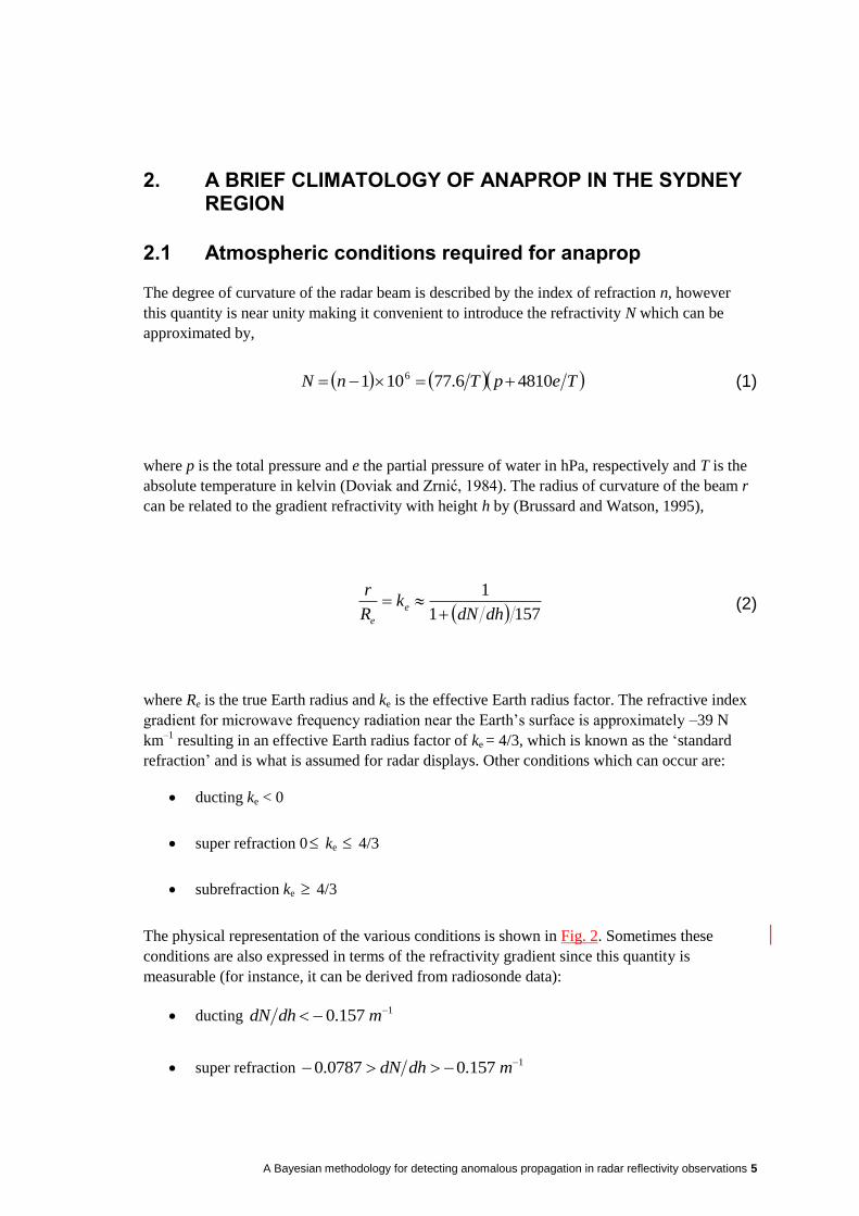
The physical representation of the various conditions is shown in Fig. 2. Sometimes these
conditions are also expressed in terms of the refractivity gradient since this quantity is
measurable (for instance, it can be derived from radiosonde data):
ducting 1157.0 mdhdN
super refraction 1157.00787.0 mdhdN
6 A Bayesian methodology for detecting anomalous propagation in radar reflectivity observations
standard refraction 10787.00 mdhdN
subrefraction 10 mdhdN
Common meteorological situations for anaprop to occur are: (1) when warm dry air from land
flows over water resulting in a near-surface temperature inversion and large increases in surface
humidity due to water vapour fluxes from the ocean, (2) within the nocturnal boundary layer
due to strong radiative cooling at the surface, (3) after the passage of cold fronts due to
humidification of the boundary layer by precipitation. The example presented in Fig. 1 was
most likely due to condition one. Such conditions are common for many coastal regions in
Australia where the majority of the population reside and many of the Bureau’s radars are
located.
Fig. 2: Schematic of the different propagation conditions of microwave radiation in the atmosphere. From
US Weather Bureau (1967)

A Bayesian methodology for detecting anomalous propagation in radar reflectivity observations 7
2.2 Datasets
The data used were from the historical record of radiosonde measurements collected at Sydney
for the period 2004–2010. Sydney was chosen as it is a major population centre in Australia and
comprises one of the ‘test-bed’ centres for the SREP project, the others being Adelaide,
Brisbane and Melbourne. Sonde releases are conducted at Sydney airport usually twice daily at
0000 UTC and 1200 UTC (1000 and 2100 EST).
The Bureau archives two sounding data products labelled as ‘significant level’ and ‘standard
level’. The standard levels are 1000, 925, 850, 700, 500, 400, 300, 250, 200, 150, 100, 70, 50,
30 and 20 hPa, which is too coarse a resolution to characterize anaprop. For instance, ducts
which form due to evaporation over the ocean are typically of the order of a few metres to a few
tens of metres deep (Brooks et al., 1999; Lenouo, 2012). The ‘significant level’ dataset is
typically 1 Hz data transmitted from the sonde, which correspond to a reading very 5–10 m for a
typical balloon ascent rate.
Fig. 3: (Left) sounding obtained at 0018 UTC (11.18 EDT) at Sydney airport. A strong temperature and
humidity inversion is present at around 980 hPa. Despite being obtained 11 hours before the PPI shown in
Fig. 1, the inversion and ducting layer persisted for many hours and was responsible the presence of
anaprop. (Right) The corresponding profile of refractivity. The delineation of conditions for ducting, super
refraction, normal refraction and sub refraction are indicated. Note the presence of many different
refractivity conditions in the lowest 5 km.
A sounding of the ‘standard level’ dataset obtained at 0018 UTC and the corresponding
refractivity profile is shown inFig. 3. It was obtained approximately 11 hours before the anaprop
present in Fig. 1, however radar images taken near the time of the sounding (not shown)
indicate a comparable amount of anaprop. A strong temperature and moisture inversion is
present below about 980 hPa as are large fluctuations in the refractivity gradient. There are
several data points with extreme negative values of refractivity gradient especially in the lowest
2 km which corresponds to the region below the temperature peak present near 900 hPa in the
sounding. Thus the region below 900 hPa is especially conducive to producing ducts.

8 A Bayesian methodology for detecting anomalous propagation in radar reflectivity observations
2.3 Prevalence of ducts
Refractivity profiles were calculated for all radiosonde soundings obtained during the period 1
January 2004 through 31 December 2009. The analysis would have been extended before this
period; however, the transmission of radiosonde data changed frequency from approximately
every five seconds to one second during 2003 which would introduce biases to the following
analysis.
The number of ducts, super-refractive and sub-refractive conditions (ducts, supref and subref,
respectively) was calculated for each category and averaged over each month. If two (or more)
consecutive (in height) measurements were found to be of one category then this was counted
only as one instance of the particular category, rather than two (or more). Furthermore, only
observations below 800 hPa were included in the calculation as ducts above this level don’t
contribute to anaprop as the angle of incidence of the radar beam to the ducting layer is too
large to be internally reflected. The results are shown in Fig. 43, and indicate a clear seasonal
cycle in the prevalence of ducts and super refractive layers with the minimum occurring during
the winter months and maximum during summer.
Fig. 4: Climatology of ducts, super refractive and sub refractive conditions at Sydney airport for the period
1 January 2004 to 31 December 2009. Only measurements below 850 hPa have been included in the
calculation.
3 We will present box plots several times in this paper as they provide a great deal of
information. The horizontal line shows the median value while the bottom and top of the box
represent the 25th and 75
th percentiles. The top and bottom of the whiskers display 1.5 times the
interquartile range of the data or roughly two standard deviations. Points below (above) the
bottom (top) of the whiskers are designated outliers. The width of the boxes is proportional to
the square root of the number of observations within the groups. Finally, the notches in the
boxes give an indication of the statistical significance of the difference between the median of
the samples; boxes in which the notches do not overlap have significantly different medians.

A Bayesian methodology for detecting anomalous propagation in radar reflectivity observations 9
Fig. 5: PDFs of the frequency of occurrence of atmospheric refractivity conditions as a function of height.
Ducts and super-refractive conditions display a greater propensity to form in the lowest ~ 30 hPa of the
atmosphere, while sub-refractive conditions show a nearly linear relationship in the lowest 200 hPa of the
atmosphere.
Histograms of the probability of occurrence of each of the refractivity categories as a function
of height (below 800 hPa) are shown in Fig. 5. Ducts are more likely to occur just near the
surface, which is particularly important as ducts at this location are more likely to result in
anaprop than those which are elevated. Super refractive conditions also are more likely to occur
just near the surface. The probabilities shown in Fig. 5 are the relative probability for each class
and not the probability of occurrence of a particular category. However, referring to Fig. 4, it
can be seen that the number of ducts, sub and super refractive conditions are approximately
equal, such that a general comparison can be made.
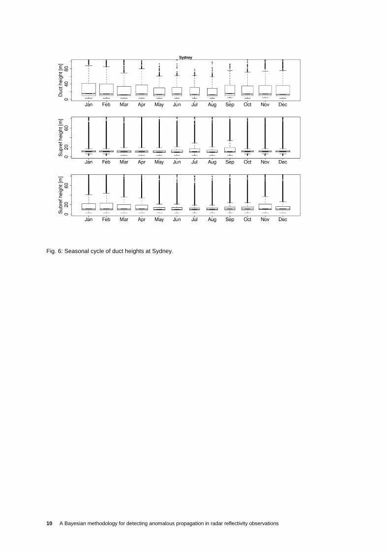
The seasonal cycle of duct heights was also calculated and is shown in Fig. 6. It shows that
ducts are generally deeper during October to March (as well as more common when compared
with Fig. 4). The enhanced prevalence and depth of ducts during the warmer months is due to
the southward progression of the subtropical high which results in strong temperature and
humidity inversions similar to the conditions shown in the sounding of Fig. 3. Often this ridge of
high pressure will form a blocking pattern in the Tasman Sea resulting in several consecutive
days with conditions conducive for ducts (Trenberth and Mo, 1985).
10 A Bayesian methodology for detecting anomalous propagation in radar reflectivity observations
Fig. 6: Seasonal cycle of duct heights at Sydney.

A Bayesian methodology for detecting anomalous propagation in radar reflectivity observations 11
3. RADAR DATA
The data were obtained with the Kurnell radar located south of Sydney at 34.01° S, 151.23° E at
an altitude of 64 m above MSL. The Kurnell radar is C-band (5 cm wavelength) with a 3 dB
beam width of 1°. The data are collected in polar coordinate format, comprising 360 azimuthal
beams each consisting of 596 range gates with a radial spacing of 250 m. The radar operating
characteristics are summarized in Table 1. Analysis was performed on polar data rather than
transformation to Cartesian coordinates. One volume, consisting of scans at eleven tilt angles
(spaced at 0.7, 1.5, 2.5, 3.5, 4.5, 5.5, 6.9, 9.2, 12.0, 15.6, 20.0 degrees) is completed in
approximately five minutes. This radar was chosen for evaluation as it covers one of Australia’s
major population centers and anaprop is a common occurrence in this location, especially
during the summer months when the prevailing subtropical high in the Tasman Sea produces
strong temperature and humidity gradients off the Australian eastern coast.
Peak power (kW) 250
Wavelength (cm) 5
Pulse repetition frequency (Hz) 1000
Pulse length (μs) 1.0
Range resolution (m) 250
Azimuthal sampling interval (°) 1
Rotation rate (°/s) 17.2
Table 1: Operating parameters for the Kurnell radar.

12 A Bayesian methodology for detecting anomalous propagation in radar reflectivity observations
4. BAYES CLUTTER CLASSIFIER
In this work a Bayes classifier is implemented to distinguish anaprop from precipitation echoes.
Bayes’ theorem (Gelman, 2004) relates the a posteriori probability of an object belonging to a
particular class c given a set of input observations nxx ,,1 and can be written as,
n
nn
xxP
cPcxxPxxcP
,
)()|,,(,,|
1
11 (3)
where ),,( 1 cxxP n is the conditional probability distribution (likelihood) of returning a
measurement xi given it belongs to class c; cP is the a priori probability of a given class and
nxxP ,,1 is the probability of obtaining a particular measurement for an input measurement
ix . The denominator in Equation (3) is constant across all classes and therefore a constant of
proportionality which can be ignored for calculations.
In this work, we implement a version of Bayes’ theorem known as the naïve Bayes classifier,
which makes the assumption that the input measurements ix are conditionally independent
which greatly simplifies the calculation of the likelihood term in Equation (3). Assuming
independence of the input measurements the likelihood term in Equation (3) can be expanded as
a multiplication of the individual conditional probabilities (Rico-Ramirez and Cluckie, 2008) so
that,
n
i in cxPcPxxcP11 )()(,, (4)
In practice the independence assumption is often violated, however, the naïve Bayes classifier
has been shown to be effective even when the independence assumption is known to be false
(e.g. Friedman et al., 1997) The conditional probabilities are obtained from training datasets
where the classification is known a priori. To obtain the a priori probability of a particular class
occurring, a climatological dataset could be used obtained to determine the probability of
each class occurring at each location. However, this would induce biases unless the dataset was
very large (in theory infinite) and instead, we make the assumption that each class is equally
likely, i.e. 5.0)()( ionprecipitatPAPP . In this instance we have defined only two
classes, however, the number of classes could be extended, and in general,
classesnocP i ./1)( . Conceptually, the problem of classification reduces to calculation of
the PDFs of the conditional probabilities for each class, while classification is determined by
maximising the a posteriori probability. For our purposes, the vector, ix corresponds to a
sequence of feature fields which can be derived from the radar observations, while the class ic
is one of anaprop or precipitation. We now turn our attention to the feature fields used as input
to the naïve Bayes classifier.

A Bayesian methodology for detecting anomalous propagation in radar reflectivity observations 13
4.1 Feature fields input to the Bayes classifier
In this section we detail the feature fields used as input to the naïve Bayes classifier. The feature
fields can be described as ‘texture-based’, which examine various bin-to-bin relationships in the
retrieved radar fields. The use of feature fields obtained from reflectivity data is advantageous
since they are numerically efficient to compute and can be implemented in post-processing
capacity, rather than requiring upgrades to radar hardware or electronics on site. The three
feature fields we will consider are; texture of reflectivity, spin and vertical profile of reflectivity.
All of these are obtained from the corrected reflectivity transmitted as a standard field from all
of the Bureau’s radars.
4.1.1 Texture of reflectivity
The texture of reflectivity (TDBZ) is a measure of the reflectivity difference between adjacent
radial reflectivity bins. It is computed as (Hubbert et al., 2009; Kessinger et al., 2004),
)(2
,1, MNdBZdBZTDBZN
j
M
i
jiji
(5)
where dBZ is the reflectivity measured in a range gate, N is the number of azimuthal radar
beams and M is the number of radial range gates; the quantity NxM is referred to as the ‘kernel’.
Texture of reflectivity is currently used in the United States WSR-88D network’s clutter
mitigation decision algorithm (Hubbert et al., 2009; Kessinger et al., 2004). These formulations
include only the radial component in the calculations, although others (e.g. Rico-Ramirez and
Cluckie, 2008) include the azimuth in calculations. Here, we use a formulation similar to that of
Hubbert et al. (2009), and average along a kernel of eleven radius gates (centred on the gate of
interest) along a single azimuth ray (i.e. N = 1 and M = 11). Evaluation of TDBZ in only the
radial component has several advantages: (1) it requires less computation time and memory
usage; (2) the radar tends to inherently average or ‘smear’ over azimuths especially at the fast
rotation rates ( ~ 17 °/s) used operationally and (3) for adjacent azimuths the distance between
measurements increases linearly with range, so that TDBZ computed in 2D has range-
dependent properties.
4.1.2 SPIN
The SPIN feature field is a measure of the number of sign changes in the relative difference of
reflectivity between adjacent reflectivity gates. The difference must be greater than a specified
threshold (nominally 2 dBZ) and the result is expressed as a percentage of all possible
fluctuations within a kernel mask (Steiner and Smith, 2002). For example, if Xi–1, Xi, and Xi+1
represent three successive gates along a radar ray, each with an associated dBZ value, then in
order for a SPIN change to occur, two conditions must be met: (1) there must be a sign change
of reflectivity either side of a specified range gate and (2) the magnitude of the average
difference between range gates preceding and following the range gate of interest must exceed a
specified threshold. Mathematically, these conditions can be expressed as (Hubbert et al., 2009),
iiii dBZdBZsigndBZdBZsign 11 (6)

14 A Bayesian methodology for detecting anomalous propagation in radar reflectivity observations
thresholdspinXXXX iiii
2
11
4.1.3 Vertical profile of reflectivity
The vertical gradient of reflectivity measures the gate-to-gate difference of the reflectivity
values between two elevation angles for the same range gate,
lu dBZdBZVPDBZ (7)
where u and l represent the upper and lower elevation angles respectively. This field is
particularly good at identifying anaprop echoes as they are normally confined to the lowest two-
to-three tilts. The Bureau’s post-processing clutter mitigation algorithm currently uses a
measure of VPDBZ to censor echoes due to anaprop, however, it has the undesired effect of
eliminating echoes from shallow stratiform precipitation. Kessinger (2004), used a range
weighting function which varied between one and zero decreasing with increasing distance from
the radar in an attempt to mitigate this problem. Since stratiform rain will have large VPDBZ
values at long distances from the radar, the weighting function is an attempt to reduce these
large values so as to not incorrectly identify stratiform rain as clutter. In the current formulation
we have not applied a range weighting function, however, it will be shown later that the current
form used for VPDBZ is sufficient when used within the framework of the naïve Bayes
classifier.
4.2 Construction of conditional PDFs from a training dataset
Application of the naïve Bayes classifier requires evaluating PDFs of the a priori conditional
probabilities for each class using training datasets. Since we are attempting to distinguish
anaprop from precipitation we specify two classes c1,2, both of which require training data. Data
representative of anaprop are presented in Fig. 1, the left hand side of which shows a plan
position indicator (PPI) radar image obtained from the lowest elevation (0.7 degrees) of the
Kurnell radar at 100 UTC 31 January 2011. The complete anaprop training dataset spanned the
time period 0000–1400 UTC which consisted of 169 volume scans comprising over 5 million
separate reflectivity returns (see Table 2).
Meteorological type Time period (UTC) No. of volumes No. of dBZ samples
Anaprop 0000–1400 169 5 089 099
Sh strat 1420–2315 107 1 405 144
Sh conv 0200–0500 37 664 291
Convect 0230–0730 61 1 007 198
Mixed 1430–2300 103 6 263 822
Table 2: Summary of time periods, number of radar volumes and number of unique reflectivity samples
used for the training dataset.

A Bayesian methodology for detecting anomalous propagation in radar reflectivity observations 15
The eastern coast of Australia is indicated by the heavy black line and many returns can be seen
emanating over the ocean. The reflectivity reaches magnitudes of 35–40 dBZ, values typical of
returns from showers at this location. These returns however, are not from precipitation but
anaprop. This is apparent on examination of the right-hand side of Fig. 1 which shows the
range-height indicator (RHI) volume slice at an azimuth of 100° clockwise from north and
reveals that returns were only present in the lowest two tilts of the volume scan. The shallow
extent of the returns is a clear indication that they are from anaprop. However, there are
occasions when heavy precipitation can occur from shallow stratiform clouds in this region; in
such situations the vertical extent of reflectivity is not necessarily a good discriminator of
anaprop and precipitation. Isolated returns (due to ‘clear-air’4 returns) were also noted to be
present to the West of the radar, however, they are of a relatively low reflectivity and are mostly
absent if a lower reflectivity threshold of 10 dBZ is applied. It was chosen to apply this
threshold to all of the training datasets as 10 dBZ is a suitable minimum reflectivity which
indicates the onset of precipitation-sized droplets (Knight and Miller, 1993). It is apparent that if
the anaprop signals were assimilated the NWP model would attempt to create precipitation
where none was present. The aim therefore, is to identify and remove echoes from anaprop.
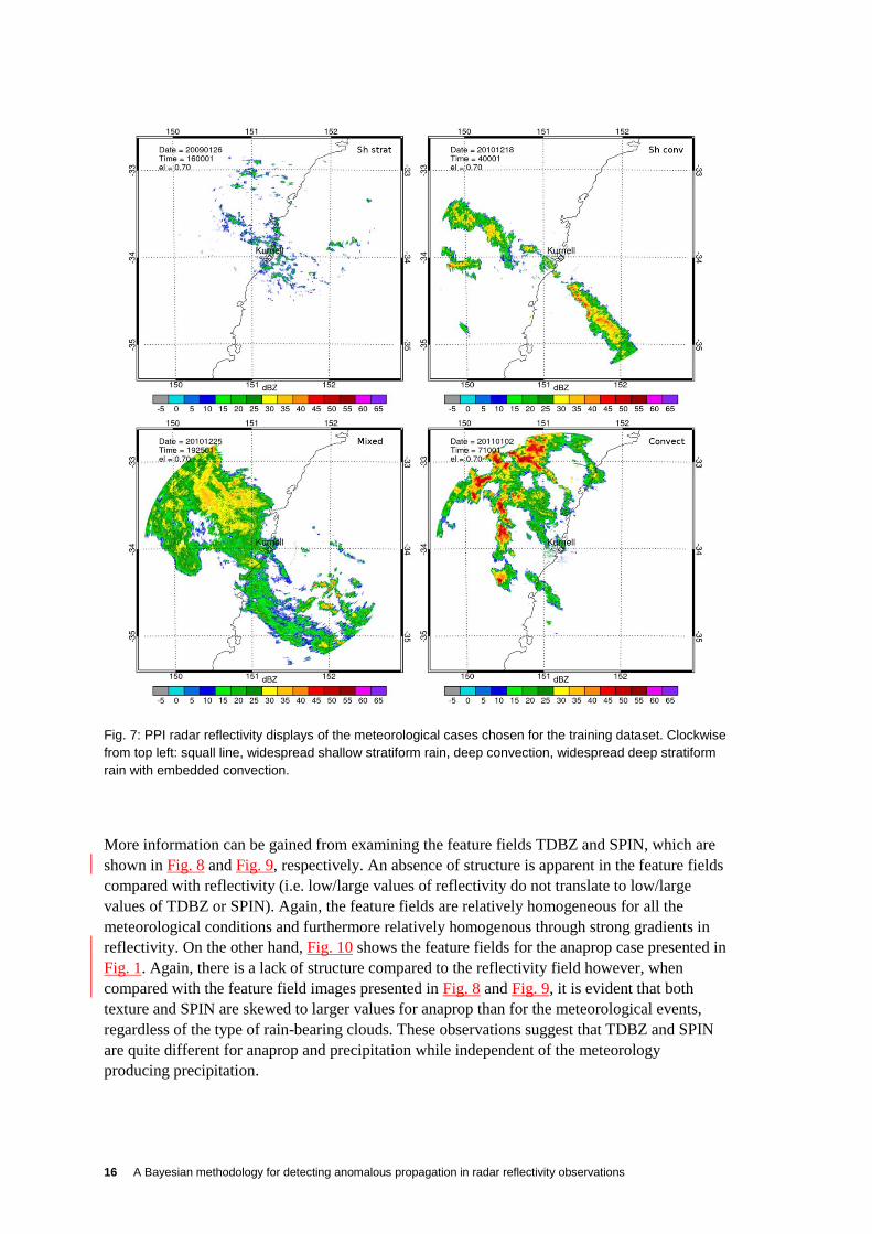
For construction of the conditional PDFs for the precipitation class, four separate precipitation
scenarios were chosen: shallow stratiform (Sh strat) rain where cloud tops were below the
freezing level and precipitation was most likely generated by warm rain processes; a line of
shallow convection (Sh conv) with cloud tops below 5 km; deep, isolated continental
convection (Conv) and widespread stratiform (Mixed) rain with embedded convective elements.
The reasons for these choices were twofold: (1) to capture a wide variety of meteorological
cases and (2) to increase sampling statistics. Radar images (PPIs) of each of the scenarios are
shown in Fig. 7. A visual comparison of the PPIs for the anaprop and shallow convection case
indicate that there is little information in the reflectivity field to distinguish them. Histograms of
reflectivity (not shown) confirm this; in fact, there is little information in the reflectivity field
(of a PPI) to distinguish each of the precipitation examples (except perhaps shallow stratiform
rain) from anaprop. Therein lies the problem of automated detection of anaprop from the
reflectivity field alone.
4 Clear-air returns are returns measured when there are no meteorological targets (i.e. clouds/rain)
present. They can be due to either (1) returns from birds, insects or (2) refractivity (humidity) gradients in
the atmosphere, which is termed Bragg scattering.
16 A Bayesian methodology for detecting anomalous propagation in radar reflectivity observations
Fig. 7: PPI radar reflectivity displays of the meteorological cases chosen for the training dataset. Clockwise
from top left: squall line, widespread shallow stratiform rain, deep convection, widespread deep stratiform
rain with embedded convection.
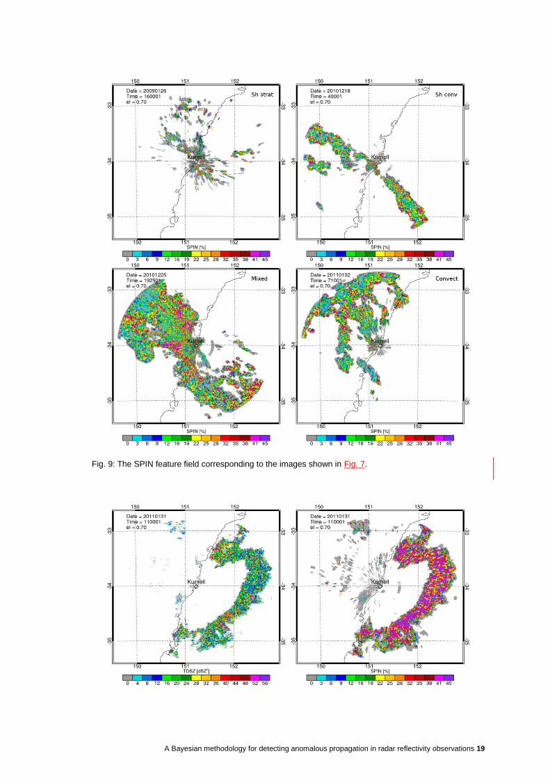
More information can be gained from examining the feature fields TDBZ and SPIN, which are
shown in Fig. 8 and Fig. 9, respectively. An absence of structure is apparent in the feature fields
compared with reflectivity (i.e. low/large values of reflectivity do not translate to low/large
values of TDBZ or SPIN). Again, the feature fields are relatively homogeneous for all the
meteorological conditions and furthermore relatively homogenous through strong gradients in
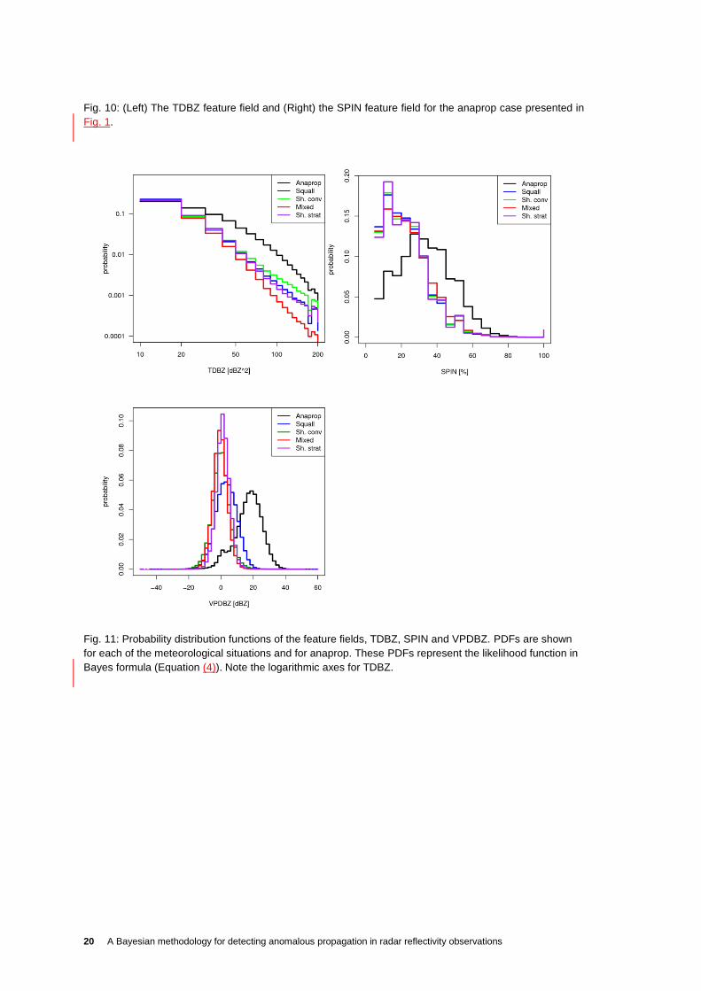
reflectivity. On the other hand, Fig. 10 shows the feature fields for the anaprop case presented in
Fig. 1. Again, there is a lack of structure compared to the reflectivity field however, when
compared with the feature field images presented in Fig. 8 and Fig. 9, it is evident that both
texture and SPIN are skewed to larger values for anaprop than for the meteorological events,
regardless of the type of rain-bearing clouds. These observations suggest that TDBZ and SPIN
are quite different for anaprop and precipitation while independent of the meteorology
producing precipitation.
A Bayesian methodology for detecting anomalous propagation in radar reflectivity observations 17
The figures show a single snapshot in time, representative of the meteorological conditions,
however, for the purposes of constructing the conditional PDFs, time periods were chosen
where the weather scenarios exemplified in Fig. 7 were applicable throughout. These periods
were chosen subjectively by examining sequences of radar images and choosing a subset of
contiguous retrievals such that the precipitation was similar (in the sense of areal extent and
type) in each volume throughout the interval. Combined the precipitation samples consisted of
308 volumes comprising over 9 million samples (see Table 2).
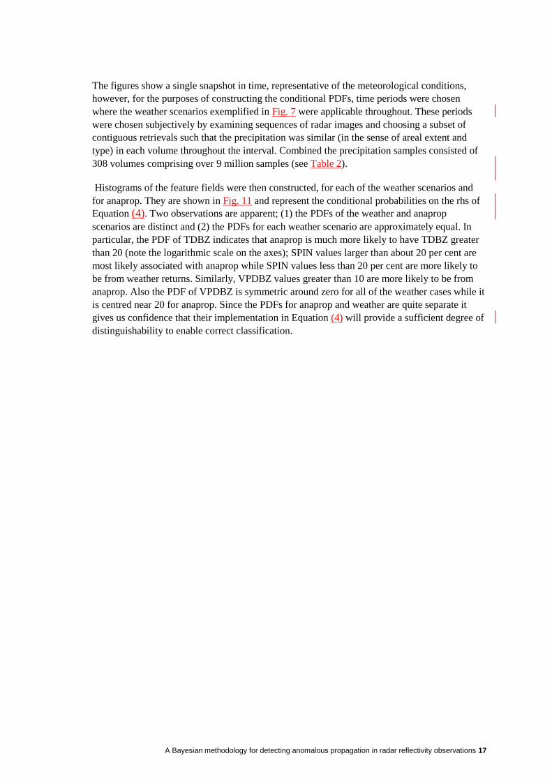
Histograms of the feature fields were then constructed, for each of the weather scenarios and
for anaprop. They are shown in Fig. 11 and represent the conditional probabilities on the rhs of
Equation (4). Two observations are apparent; (1) the PDFs of the weather and anaprop
scenarios are distinct and (2) the PDFs for each weather scenario are approximately equal. In
particular, the PDF of TDBZ indicates that anaprop is much more likely to have TDBZ greater
than 20 (note the logarithmic scale on the axes); SPIN values larger than about 20 per cent are
most likely associated with anaprop while SPIN values less than 20 per cent are more likely to
be from weather returns. Similarly, VPDBZ values greater than 10 are more likely to be from
anaprop. Also the PDF of VPDBZ is symmetric around zero for all of the weather cases while it
is centred near 20 for anaprop. Since the PDFs for anaprop and weather are quite separate it
gives us confidence that their implementation in Equation (4) will provide a sufficient degree of
distinguishability to enable correct classification.

18 A Bayesian methodology for detecting anomalous propagation in radar reflectivity observations
Fig. 8: The texture feature field (TDBZ) corresponding to the images shown in Fig. 7.
A Bayesian methodology for detecting anomalous propagation in radar reflectivity observations 19
Fig. 9: The SPIN feature field corresponding to the images shown in Fig. 7.
20 A Bayesian methodology for detecting anomalous propagation in radar reflectivity observations
Fig. 10: (Left) The TDBZ feature field and (Right) the SPIN feature field for the anaprop case presented in
Fig. 1.
Fig. 11: Probability distribution functions of the feature fields, TDBZ, SPIN and VPDBZ. PDFs are shown
for each of the meteorological situations and for anaprop. These PDFs represent the likelihood function in
Bayes formula (Equation (4)). Note the logarithmic axes for TDBZ.
A Bayesian methodology for detecting anomalous propagation in radar reflectivity observations 21
4.3 Transformation of the conditional PDFs
The conditional PDFs as shown in the above section could be used for the naïve Bayes classifier
but their implementation would require the use of a look-up table. For instance, the feature
fields could be evaluated and a probability determined (via the look-up table) of that
measurement occurring based on whether the classification was that of anaprop or precipitation.
For operational purposes, this is unfeasible due to computational limitations. To facilitate
implementation of the classifier in an operational setting, it would be beneficial if the
conditional probability distributions presented in Fig. 11 were parameterised by a mathematical
function. For instance, if the PDFs were described by a Gaussian distribution then they could be
completely described by the mean and standard deviation requiring minimal computation. To
this end, power transforms of the conditional PDFs, provide a possible technique to make the
data more normal distribution-like. There are many possible transforms but one which is well-
established within the statistical literature is that of the Box–Cox transformation. It provides a
transform which transforms data to a Gaussian or normal distribution. The Box–Cox
transformation is,
.0if,y log
;0 if,1
)(
y
y (8)
where y is a measured variable and is the transformation parameter. The value of is
determined by maximising the logarithm of the likelihood function (Wilks, 2011),
i
n
=i
n
=i
i yλ+n
λyλyn=λy,f
11
2
ln1ln2
(9)
where )(y is the arithmetic mean of the data. In this case, y corresponds to a vector of
observations 321 ,, yyyy
where the elements of the vector are given by the feature fields.
The PDF for VPDBZ is approximately normal (see Fig. 11) and so the transformation was only
applied to the TDBZ and SPIN feature fields.
The log-likelihood function for the TDBZ and SPIN feature fields were evaluated and the
calculations for the TDBZ field of anaprop are shown in Fig. 12. The maximum of this
parabolic function provides the optimal value of for insertion to Equation (8) so as to
transform the PDFs shown in Fig. 11 to approximately normal distributions. Similar
calculations were performed for all meteorological scenarios and each feature field. The results
are summarised in Table 3. Since it is not known a priori what the prevailing meteorology is, an
average value applicable to all precipitation cases weather , was evaluated. These values are listed
in the rhs column of Table 3 and were used to transform the conditional PDFs of Fig. 11 via
Equation (8).

22 A Bayesian methodology for detecting anomalous propagation in radar reflectivity observations
Fig. 12: The log-likelihood as a function of λ (see Equation (9)). The value of λ which maximizes the log-
likelihood function provides the best value to transform the data to an approximately normal distribution via
Equation (8)). The dotted lines represent the 95 per cent confidence interval for λ. This curve is the log-
likelihood function evaluated for the TDBZ field of the anaprop case. Values for TDBZ and SPIN for each
case are presented in Table 3.
Anaprop Sh strat Sh conv Convect Mixed ionprecipitat
TDBZ –0.11 –0.34 –0.2 –0.22 –0.24 –0.25
SPIN 0.3 0.25 0.25 0.26 0.29 0.26
Table 3: Calculated values of λ for the Box–Cox transformation described by Equation (8) for anaprop and
each of the precipitation cases. The last column shows the average value of λ for all precipitation cases
combined.
The resulting transformed PDFs are shown in Fig. 13. As was found prior to application of the
Box–Cox transformation, the PDFs are approximately equal for all precipitation scenarios and
they are distinct from anaprop for both TDBZ and SPIN. It is also noted that the Box–Cox
transformation has been successful at transforming the PDFs to approximately normal
A Bayesian methodology for detecting anomalous propagation in radar reflectivity observations 23
distributions. The original TDBZ and SPIN fields were re-evaluated from the training dataset
and the Box–Cox transformation applied to it. The mean (μ) and unbiased estimate of the
standard deviation (σ) of the data were then evaluated via a two-pass algorithm,
1
)(1
2
1
n
x
nx
n
i i
n
i i
(10)
Fig. 13: Probability distribution functions of the feature fields TDBZ and SPIN after transformation
according to the Box–Cox power law given by Equation (8). Note that the distributions are now
approximately normal.
These values summarized in Table 4. The Gaussian distributions described by these two
parameters were calculated and are plotted in Fig. 14, and overlaid with the histograms of Fig.
13. The Gaussian distributions calculated directly from the mean and unbiased estimate of the
standard deviation of the data very closely overlay the PDFs of the original data and therefore,
to a close approximation, the conditional PDFs can be parameterized via the mean and unbiased
estimate of the standard deviation of the Box–Cox transformation of the respective feature
fields. We label these feature fields BCTDBZ and BCSPIN.
Anaprop Precipitation
μ σ μ σ
BCTDBZ 2.6 0.62 1.69 0.45
BCSPIN 5.96 1.42 4.71 1.24
VPDBZ 16.69 8.49 0.74 5.30
Table 4: Mean (μ) and unbiased estimate of the standard deviation (σ) of the feature fields for anaprop and
precipitation. The values in the precipitation column are an average of each of the precipitation scenarios.

24 A Bayesian methodology for detecting anomalous propagation in radar reflectivity observations
They were obtained by applying the Box–Cox transformation to the feature fields of the training data and
then computing μ and σ of the transformed distribution.
Fig. 14: Same as Fig. 13 including the best-fit normal curves determined from the mean and unbiased
estimate of the standard deviation of the Box–Cox transformed training datasets.
4.4 Independence of the feature fields
The linear independence of the input feature fields is one of the key assumptions of the NBC.
Despite this assumption it has been proven to be effective even when the assumption of
independence is violated (e.g. Friedman et al., 1997). However, it is worthwhile to examine the
independence assumption between each of the feature fields. Scatter plots of each combination
of the transformed feature fields are shown in Fig. 15, and it can be seen that there is some
degree of correlation between each of the feature fields.
Fig. 15: Scatter plots of each of the Box–Cox transformed variables. Values for precipitation are shown in
grey while anaprop values are in black. As for Fig. 14, the values for anaprop are separated from those for
precipitation.
To quantify the magnitude of the correlation, Pearson’s correlation coefficients were calculated
for each combination of the original and Box–Cox transformed feature fields. The results are
summarised in Table 5. The VPDBZ field is either uncorrelated or very weakly correlated with
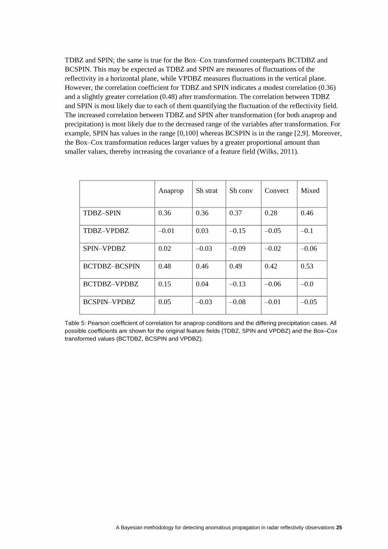
A Bayesian methodology for detecting anomalous propagation in radar reflectivity observations 25
TDBZ and SPIN; the same is true for the Box–Cox transformed counterparts BCTDBZ and
BCSPIN. This may be expected as TDBZ and SPIN are measures of fluctuations of the
reflectivity in a horizontal plane, while VPDBZ measures fluctuations in the vertical plane.
However, the correlation coefficient for TDBZ and SPIN indicates a modest correlation (0.36)
and a slightly greater correlation (0.48) after transformation. The correlation between TDBZ
and SPIN is most likely due to each of them quantifying the fluctuation of the reflectivity field.
The increased correlation between TDBZ and SPIN after transformation (for both anaprop and
precipitation) is most likely due to the decreased range of the variables after transformation. For
example, SPIN has values in the range [0,100] whereas BCSPIN is in the range [2,9]. Moreover,
the Box–Cox transformation reduces larger values by a greater proportional amount than
smaller values, thereby increasing the covariance of a feature field (Wilks, 2011).
Anaprop Sh strat Sh conv Convect Mixed
TDBZ–SPIN 0.36 0.36 0.37 0.28 0.46
TDBZ–VPDBZ –0.01 0.03 –0.15 –0.05 –0.1
SPIN–VPDBZ 0.02 –0.03 –0.09 –0.02 –0.06
BCTDBZ–BCSPIN 0.48 0.46 0.49 0.42 0.53
BCTDBZ–VPDBZ 0.15 0.04 –0.13 –0.06 –0.0
BCSPIN–VPDBZ 0.05 –0.03 –0.08 –0.01 –0.05
Table 5: Pearson coefficient of correlation for anaprop conditions and the differing precipitation cases. All
possible coefficients are shown for the original feature fields (TDBZ, SPIN and VPDBZ) and the Box–Cox
transformed values (BCTDBZ, BCSPIN and VPDBZ).
26 A Bayesian methodology for detecting anomalous propagation in radar reflectivity observations
5. RESULTS
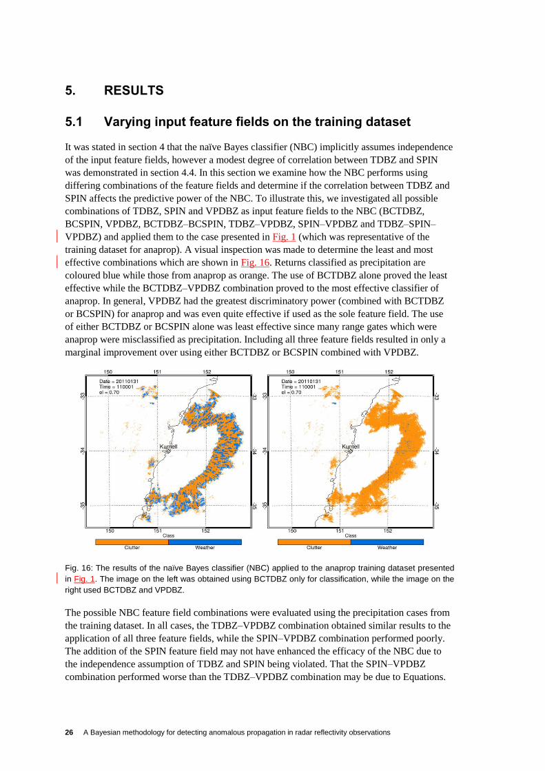
5.1 Varying input feature fields on the training dataset
It was stated in section 4 that the naïve Bayes classifier (NBC) implicitly assumes independence
of the input feature fields, however a modest degree of correlation between TDBZ and SPIN
was demonstrated in section 4.4. In this section we examine how the NBC performs using
differing combinations of the feature fields and determine if the correlation between TDBZ and
SPIN affects the predictive power of the NBC. To illustrate this, we investigated all possible
combinations of TDBZ, SPIN and VPDBZ as input feature fields to the NBC (BCTDBZ,
BCSPIN, VPDBZ, BCTDBZ–BCSPIN, TDBZ–VPDBZ, SPIN–VPDBZ and TDBZ–SPIN–
VPDBZ) and applied them to the case presented in Fig. 1 (which was representative of the
training dataset for anaprop). A visual inspection was made to determine the least and most
effective combinations which are shown in Fig. 16. Returns classified as precipitation are
coloured blue while those from anaprop as orange. The use of BCTDBZ alone proved the least
effective while the BCTDBZ–VPDBZ combination proved to the most effective classifier of
anaprop. In general, VPDBZ had the greatest discriminatory power (combined with BCTDBZ
or BCSPIN) for anaprop and was even quite effective if used as the sole feature field. The use
of either BCTDBZ or BCSPIN alone was least effective since many range gates which were
anaprop were misclassified as precipitation. Including all three feature fields resulted in only a
marginal improvement over using either BCTDBZ or BCSPIN combined with VPDBZ.
Fig. 16: The results of the naïve Bayes classifier (NBC) applied to the anaprop training dataset presented
in Fig. 1. The image on the left was obtained using BCTDBZ only for classification, while the image on the
right used BCTDBZ and VPDBZ.
The possible NBC feature field combinations were evaluated using the precipitation cases from
the training dataset. In all cases, the TDBZ–VPDBZ combination obtained similar results to the
application of all three feature fields, while the SPIN–VPDBZ combination performed poorly.
The addition of the SPIN feature field may not have enhanced the efficacy of the NBC due to
the independence assumption of TDBZ and SPIN being violated. That the SPIN–VPDBZ
combination performed worse than the TDBZ–VPDBZ combination may be due to Equations.

A Bayesian methodology for detecting anomalous propagation in radar reflectivity observations 27
(5) and (6) being evaluated in only the radial direction. A kernel size of 20 was chosen, so as to
allow a sufficient dynamic range in the evaluation of the SPIN (a kernel size of 20 will give a
minimum discrete interval of 5 per cent in the evaluation of SPIN). However, a kernel size of 20
equates to a radial range of 5 km, which may have the unintended consequence of smearing
over precipitation and non-precipitation pixels. The inclusion of azimuths in the evaluation of
SPIN, which will enable the kernel size to be kept the same while decreasing the radial extent,
is needed to evaluate the effectiveness of evaluating SPIN in one dimension only. Despite this,
it appeared that using TDBZ and VPDBZ gave similar results to the application of all three
feature fields and for this reason the BCTDBZ–VPDBZ combination will be used to present the
NBC results herein.
The image which was transmitted for public display by the Bureau corresponding to the anaprop
presented in Fig. 1 is shown in the left-hand side of Fig. 17. The NBC provides a substantial
improvement over the current clutter mitigation system employed at the Bureau, which uses
basic thresholds of reflectivity and vertical height to censor data. However, in the image shown,
the reflectivity and height thresholds were exceeded allowing incorrect radar returns to be
included. The problem becomes more pronounced at greater distances from the radar because
beam propagation causes the beam to be above the minimum height threshold once a certain
range is reached.
Fig. 17: Images transmitted for public display using the Bureau’s current clutter mitigation system. The
images correspond to the anaprop data presented in Fig. 1 and the shallow stratiform case presented in
Fig. 7. It can be seen that the current system is ineffective at removing anaprop, especially far from the
radar, while it also removes many genuine precipitation pixels, especially close to the radar.

28 A Bayesian methodology for detecting anomalous propagation in radar reflectivity observations
5.2 Verification of the classifier
After conducting a visual evaluation of the best combination of feature fields to input to the
NBC the performance of the NBC was quantified. To achieve this we applied the NBC to each
of the training datasets, which we assumed a priori consisted entirely of either anaprop or
precipitation samples. These data were used to construct the conditional probability PDFs (see
Fig. 11, Fig. 13 and Fig. 14), therefore, if the NBC was perfect, would classify each pixel
correctly. The total number of pixels classified as either anaprop or precipitation was calculated
for each of the training datasets and the results are presented as a contingency table in Table 6.
The numbers differ from those in Table 2 because all of the pixels in a volume were used to
construct the contingency table, while only those from the lowest tilt were used to train the
NBC. The raw values are presented above and the proportional values below in parentheses.
There are many different ‘skill scores’ which can be derived from the contingency table;
however, the dimensionality of the table is three and all the information contained in it can be
summarized with three statistics (Wilks, 2011). Three which are commonly used are the hit rate
( caaH ), the false alarm rate ( dbbF ) and the base rate ( cP – or sample
climatological relative frequency) of the class in question. Each of these scalar attributes can be
quoted for each class (i.e. anaprop or precipitation) but we will quote only the values for
anaprop: H = 0.981, F = 0.098, P(c) = 0.095. This means that about 98 per cent of anaprop
pixels were correctly detected and about ten per cent of the precipitation pixels were
misclassified as anaprop. The sample climatological relative frequency of anaprop was about
ten per cent, which is probably substantially larger than the actual climatological frequency of
anaprop. In other words, the NBC is very good (98 per cent) at classifying anaprop correctly
however, ten per cent of the time it incorrectly classifies a precipitation pixel as anaprop. For
the purposes of QPE or NWP assimilation this is a more desirable characteristic than the
opposite (i.e. misclassifying ten per cent of anaprop as precipitation).
Observed
NB
C c
lass
ific
atio
n
Anaprop Precip. Marginal Totals
(forecasts)
Anaprop 6 267 195
(0.047)
5 927 313
(0.044)
12 194 508
(0.091)
Precip. 120 005
(9×10⁻⁴
)
54 680 422
(0.410)
54 800 427
(0.410)
Marginal totals
(observed)
6 387 200
(0.048)
60 607 735
(0.452)
Total no. samples
133 989 870
Table 6: Contingency table constructed from the anaprop and precipitation training datasets. A minimum
reflectivity threshold of 10 dBZ was applied.

A Bayesian methodology for detecting anomalous propagation in radar reflectivity observations 29
5.3 Application to the training dataset precipitation cases
The results of applying the NBC to the precipitation cases, using the BCTDBZ–VPDBZ feature
fields as discriminators, are shown in Fig. 18. For the shallow stratocumulus case (top left) the
NBC has identified most (~70 per cent) reflectivities larger than about 15 dBZ as precipitation.
The formation of precipitation-sized droplets is indicated at radar reflectivities of about 5–10
dBZ for a C-band radar (Knight and Miller, 1993), so the NBC has been particularly effective at
identifying the shallow precipitation bands within these stratocumulus. We also note that the
current method employed at the Bureau to eliminate anaprop, which relies solely on examining
the vertical profile of reflectivity, rejected these echoes in near entirety as anaprop (see right-
hand side of Fig. 17). This was because the precipitation was mainly confined below the height
threshold designed to eliminate anaprop. The NBC represents a substantial improvement for the
identification of shallow precipitation, which will improve QPE calculations. Shallow cumulus
convection is also well distinguished however, some precipitation echoes, especially those at the
edge of the radar volume, have been incorrectly classified as anaprop. This is due to the spread
of the radar beam with distance and the use of VPDBZ as a classifier. In this case cloud top
height was between 4–5 km and at large distances from the radar, two vertically-aligned range
gates were sufficiently large to overshoot cloud top, resulting in a large VPDBZ value, typical
of anaprop (see Fig. 11). We note that the NBC using BCTDBZ only as the input feature field
identified all of the returns as precipitation suggesting that, in the case of shallow precipitation,
the use of BCTDBZ alone may perform better. The inclusion of BCSPIN degraded the
performance of the NBC. However, since it is not known a priori what the source of returns is
and the NBC cannot adapt its input feature fields accordingly, the use of the most effective
combination over all precipitation types (BCTDBZ–VPDBZ) is preferable. The classification of
the deeper precipitation, whether stratus or convective in nature (Convect and Mixed), has been
partially (88 per cent and 94 per cent, respectively) successful and is acceptable for the purposes
of data assimilation or QPE/QPF. Given that the current numerical weather prediction model
used at the Bureau —the Australian Community Earth Climate System Simulator (ACCESS)
(Puri et al., 2012)— has a grid spacing of 5 km, the raw radar reflectivity needs to be thinned
(using ‘superobservations’) so this accuracy is most likely suitable for data assimilation or
QPE/QPF (Weng and Zhang, 2011), although this requires further investigation

30 A Bayesian methodology for detecting anomalous propagation in radar reflectivity observations
Fig. 18: The results of the NBC applied to the precipitation cases from the training dataset. The original
reflectivity images are shown in Fig. 7.
5.4 Application to a case of rain embedded in anaprop
We now evaluate the NBC on a case other than the training dataset. Consider Fig. 19, which is a
particularly interesting example as the image contains returns from both anaprop and
precipitation. The returns in the northeast quadrant of the image are from anaprop while those in
the southeast are from convective storms. This becomes apparent when examining the PPI
obtained at the second radar elevation (top right), where the returns originating from anaprop
have disappeared as the radar beam is no longer internally reflected at the temperature and
humidity inversion. This is further emphasized when the RHIs at 40° and 112° are examined;
the RHI at 40° only has returns in the lowest elevation, while the RHI at 112° indicates the
presence of a well-developed convective storm containing reflectivities greater than 25 dBZ
extending above 7 km. The simultaneous presence of both anaprop and precipitation in the same
image provides a useful example with which to evaluate the efficacy of the NBC.

A Bayesian methodology for detecting anomalous propagation in radar reflectivity observations 31
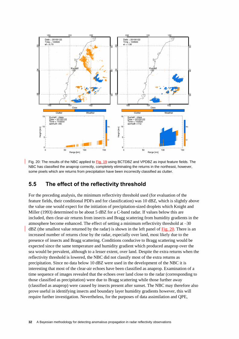
Fig. 20 shows the results of applying the NBC to this scene using BCTDBZ and VPDBZ as
input feature fields. The PPI images (top row) show that the NBC is effective at distinguishing
anaprop from precipitation, however, some precipitation pixels have been misclassified as
anaprop. This is further illustrated by the RHI images (bottom row), again at 40° and 112°
which indicate that while the NBC has positively identified anaprop some precipitation signals
have been misclassified.
Fig. 19: An example of anaprop and a convective storm obtained from the Kurnell radar on 22 January
2010. Anaprop is present in the northeast and a convective storm in the southeast. The top left panel is a
PPI image obtained at the lowest elevation (0.7°), while the top right panel was obtained at the next
highest elevation (1.5°). Note the absence of anaprop in the higher elevation. The bottom left panel is an
RHI obtained at an azimuth of 40° through the anaprop, while the lower right panel is an RHI at 112° and
shows the presence of a convective system extending to nearly 10 km height. The azimuths of the RHIs
are indicated by the black line in the PPIs.
32 A Bayesian methodology for detecting anomalous propagation in radar reflectivity observations
Fig. 20: The results of the NBC applied to Fig. 19 using BCTDBZ and VPDBZ as input feature fields. The
NBC has classified the anaprop correctly, completely eliminating the returns in the northeast, however,
some pixels which are returns from precipitation have been incorrectly classified as clutter.
5.5 The effect of the reflectivity threshold
For the preceding analysis, the minimum reflectivity threshold used (for evaluation of the
feature fields, their conditional PDFs and for classification) was 10 dBZ, which is slightly above
the value one would expect for the initiation of precipitation-sized droplets which Knight and
Miller (1993) determined to be about 5 dBZ for a C-band radar. If values below this are
included, then clear-air returns from insects and Bragg scattering from humidity gradients in the
atmosphere become enhanced. The effect of setting a minimum reflectivity threshold at –30
dBZ (the smallest value returned by the radar) is shown in the left panel of Fig. 20. There is an
increased number of returns close by the radar, especially over land, most likely due to the
presence of insects and Bragg scattering. Conditions conducive to Bragg scattering would be
expected since the same temperature and humidity gradient which produced anaprop over the
sea would be prevalent, although to a lesser extent, over land. Despite the extra returns when the
reflectivity threshold is lowered, the NBC did not classify most of the extra returns as
precipitation. Since no data below 10 dBZ were used in the development of the NBC it is
interesting that most of the clear-air echoes have been classified as anaprop. Examination of a
time sequence of images revealed that the echoes over land close to the radar (corresponding to
those classified as precipitation) were due to Bragg scattering while those further away
(classified as anaprop) were caused by insects present after sunset. The NBC may therefore also
prove useful in identifying insects and boundary layer humidity gradients however, this will
require further investigation. Nevertheless, for the purposes of data assimilation and QPE,

A Bayesian methodology for detecting anomalous propagation in radar reflectivity observations 33
setting a reflectivity threshold near 10 dBZ is advisable and mitigates this problem. However,
the use of the Doppler wind field (e.g.Rennie et al., 2010) is advisable to identify insect echoes
and such research is being undertaken concurrently at the Bureau. Furthermore, software is
being developed within the Bureau which will enable selecting regions of interest, and
subjectively defining an a priori class to them to determine if and how PDFs of feature fields
for insects (for instance) differ from those of anaprop.
Fig. 21: (left) PPI image of mixed anaprop and precipitation using a minimum reflectivity threshold of −30
dBZ. Note the increase in returns over land close to the radar compared to Fig. 19. These returns were
most likely due to Bragg scattering. (right) Results of the NBC using −30 dBZ as the minimum reflectivity
threshold.
5.6 Application to radars other than Kurnell
It is feasible that the texture and SPIN variables may be sensitive to radar operating
characteristics such as wavelength and beamwidth. The Kurnell radar is ideally situated to test
this hypothesis as two Bureau radars are located to the north and south of it each with differing
operating characteristics. The Terrey Hills radar is an S-band (10 cm), 1° beamwidth radar
located about 40 km to the north of the Kurnell radar, while the Wollongong radar is an S-band,
2° beamwidth radar located about 55 km to the south. Comprised, the radars are a combination
of 5 and 10 cm wavelength and 1 and 2 degree beamwidth operating parameters.
Fig. 22 is an example of shallow convection and anaprop observed by each of the radars at
approximately the same time. The same gross features are evident with many convective
elements present over the ocean. The convection was very shallow and confined mostly below 4
km altitude. Consider the small convective element just east of the Kurnell radar which is
circled. It is clearly visible in all three radars; however, more anaprop is evident in the Kurnell
and Wollongong radar images. Fig. 23 shows the results of applying the NBC to the PPIs. It can
be seen that the anaprop surrounding the convection in the Kurnell and Wollongong images has
been correctly distinguished. It is encouraging that the NBC has managed to perform well when

34 A Bayesian methodology for detecting anomalous propagation in radar reflectivity observations
applied to radars with different operating characteristics, and gives us confidence that the NBC
can be directly applied to other radars around the country.
It is unclear why more anaprop is present in the Kurnell and Wollongong radars compared to
Terry Hills. It may be due to the altitude of the radar, however, Terry Hills is at an altitude
midway between the other two indicating no obvious decrease in anaprop as a function of
height of the radar as may be expected. The radar beamwidth may be a contributing factor since
Wollongong (with a 2° beamwidth) exhibits a greater amount of anaprop compared with the
other two radars. In particular, tests of the NBC on radars at other locations around Australia
reveal that the feature fields may be susceptible to beamwidth and range resolution. Another
factor which may influence the NBC, however, may be the climatic region for which it was
tuned i.e. it may not perform so well in the tropical north of the country or in the temperate
regions further south. This point needs further examination and will be the focus of future
studies.
Fig. 22: An example of anaprop and shallow maritime cumulus convection observed from three separate
radars: Terrey Hills, Kurnell and Wollongong) each with different operating characteristics.
Fig. 23: The NBC applied to the PPIs from Fig. 22
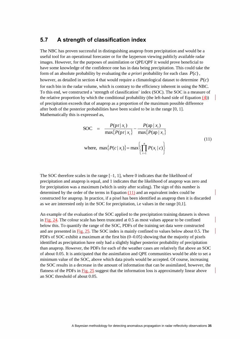
A Bayesian methodology for detecting anomalous propagation in radar reflectivity observations 35
5.7 A strength of classification index
The NBC has proven successful in distinguishing anaprop from precipitation and would be a
useful tool for an operational forecaster or for the layperson viewing publicly available radar
images. However, for the purposes of assimilation or QPE/QPF it would prove beneficial to
have some knowledge of the confidence one has in data being precipitation. This could take the
form of an absolute probability by evaluating the a priori probability for each class )(cP ,
however, as detailed in section 4 that would require a climatological dataset to determine )(cP
for each bin in the radar volume, which is contrary to the efficiency inherent in using the NBC.
To this end, we constructed a ‘strength of classification’ index (SOC). The SOC is a measure of
the relative proportion by which the conditional probability (the left-hand side of Equation (4))
of precipitation exceeds that of anaprop as a proportion of the maximum possible difference
after both of the posterior probabilities have been scaled to be in the range [0, 1].
Mathematically this is expressed as,
ii
i
i
xP
xP
xP
xP
|ap(max
)|ap(
|pr(max
)|pr(SOC
n
i
ii cxPxcP1
)|(max)|(max where,
(11)
The SOC therefore scales in the range [–1, 1], where 0 indicates that the likelihood of
precipitation and anaprop is equal, and 1 indicates that the likelihood of anaprop was zero and
for precipitation was a maximum (which is unity after scaling). The sign of this number is
determined by the order of the terms in Equation (11) and an equivalent index could be
constructed for anaprop. In practice, if a pixel has been identified as anaprop then it is discarded
as we are interested only in the SOC for precipitation, i.e values in the range [0,1].
An example of the evaluation of the SOC applied to the precipitation training datasets is shown
in Fig. 24. The colour scale has been truncated at 0.5 as most values appear to be confined
below this. To quantify the range of the SOC, PDFs of the training set data were constructed
and are presented in Fig. 25. The SOC index is mainly confined to values below about 0.5. The
PDFs of SOC exhibit a maximum at the first bin (0–0.05) showing that the majority of pixels
identified as precipitation have only had a slightly higher posterior probability of precipitation
than anaprop. However, the PDFs for each of the weather cases are relatively flat above an SOC
of about 0.05. It is anticipated that the assimilation and QPE communities would be able to set a
minimum value of the SOC, above which data pixels would be accepted. Of course, increasing
the SOC results in a decrease in the amount of information that can be assimilated, however, the
flatness of the PDFs in Fig. 25 suggest that the information loss is approximately linear above
an SOC threshold of about 0.05.
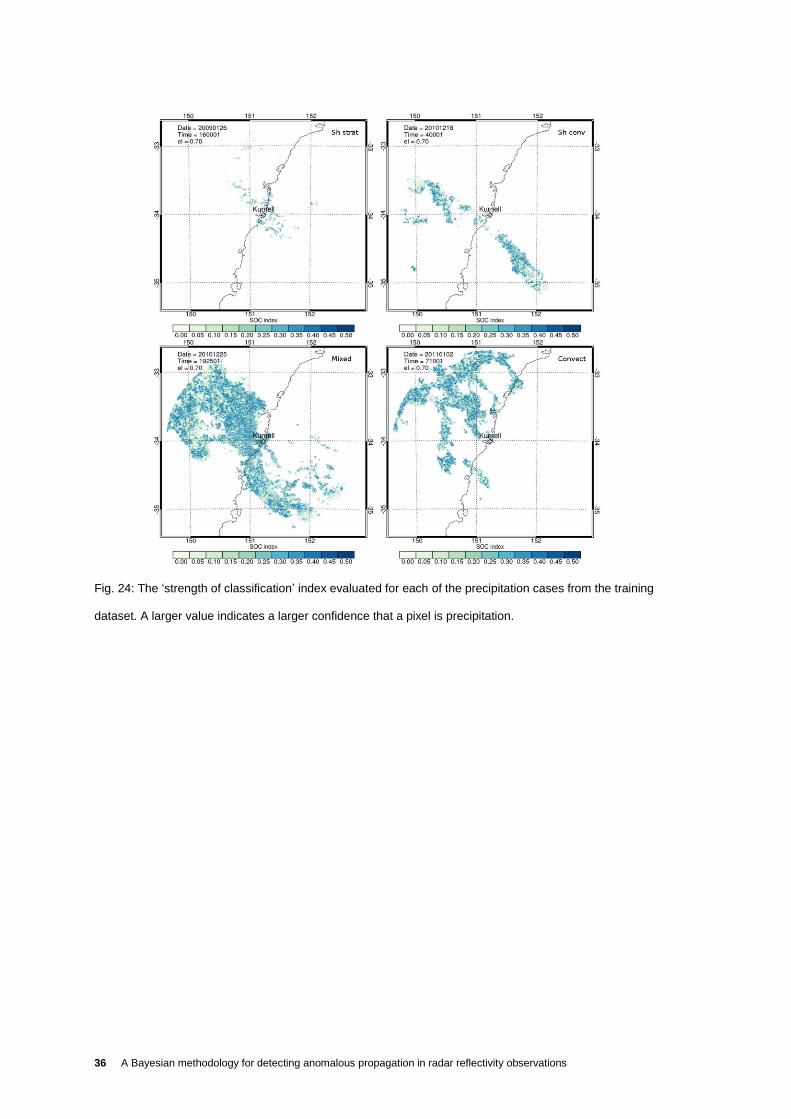
36 A Bayesian methodology for detecting anomalous propagation in radar reflectivity observations
Fig. 24: The ‘strength of classification’ index evaluated for each of the precipitation cases from the training
dataset. A larger value indicates a larger confidence that a pixel is precipitation.
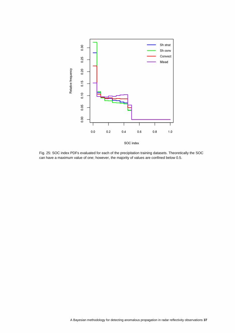
A Bayesian methodology for detecting anomalous propagation in radar reflectivity observations 37
Fig. 25: SOC index PDFs evaluated for each of the precipitation training datasets. Theoretically the SOC
can have a maximum value of one; however, the majority of values are confined below 0.5.

38 A Bayesian methodology for detecting anomalous propagation in radar reflectivity observations
6. SUMMARY AND CONCLUSIONS
In this study a naïve Bayes classifier (NBC) was developed and tested. The NBC is an extension
of Bayes’ theorem which classifies radar echoes into two classes, 21 and cc , based on a series of
feature vectors, nxx ,,1 , by maximizing the a posteriori probability )( ii xcp . The classes were
designated to be either anomalous propagation (anaprop) or precipitation and the feature fields
investigated were texture of reflectivity (TDBZ), spin change variable (SPIN) (Steiner and
Smith, 2002) and vertical profile of reflectivity (VPDBZ).
The NBC is a supervised learning technique, which requires a training dataset of examples in
which the classification is known a priori. The training dataset consisted of five subclasses—
one of anaprop and four distinct precipitation regimes; shallow stratiform, shallow convection,
deep convection and deep stratiform precipitation with embedded convection. Probability
distribution functions (PDFs) of the feature fields were evaluated for anaprop and each of the
precipitation subclasses. The PDFs of the precipitation subclasses were found to be similar
despite distinct meteorological forcing mechanisms. Moreover, the PDFs of the feature fields
for anaprop were distinct from the PDFs of the precipitation subclasses, suggesting that they
convey information which allows categorisation of precipitation and anaprop.
The feature field PDFs were found to be non-normal which, if used in their native form, would
require the use of look-up tables to evaluate the conditional probability in Bayes’ theorem. To
parameterise the conditional PDFs they were transformed to approximately normal distributions
via a Box–Cox transformation, which allowed them to be specified completely via the mean and
standard deviation.
All (seven) possible combinations of the feature fields were investigated on the training datasets
to evaluate the most effective combination, which was found to be TDBZ and VPDBZ. The use
of all three feature fields did not, as a rule, add any benefit to the NBC and in some cases caused
it to perform worse. This was attributed to TDBZ and SPIN not being linearly independent as
they are both measures of the variability of the reflectivity field. When considered individually,
VPDBZ was found to be the most effective feature field at distinguishing anaprop from
precipitation.
The NBC was then applied to an independent case where precipitation and anaprop were
present in the same region. The BCTDBZ–VPDBZ combination of feature fields proved most
effective at classifying pixels correctly. Some pixels were incorrectly classified, but given the
current data resolution required for purposes of data assimilation or QPE these errors were
considered minimal. Some sensitivity to the reflectivity threshold was found, whereby returns
from clear air appeared as the threshold was decreased. However, when the threshold was set at
a reasonable level to distinguish most clear-air returns from the smallest precipitation-sized
drops, (around 5 dBZ for a C-band radar) this problem was circumvented. The NBC however,
shows some promise in being able to distinguish Bragg echoes from insect echoes. Furthermore,
the NBC performed well when applied to the Terrey Hills and Wollongong radars, which means
that the PDFs of texture and SPIN feature fields are most likely independent of radar operating
parameters such as wavelength and beamwidth. However, the NBC was not tested on radars in
differing climatic zones which will be the subject of future research.

A Bayesian methodology for detecting anomalous propagation in radar reflectivity observations 39
The NBC was extended via a ‘strength of classification’ index (SOC), which was constructed as
a measure of the confidence with which a pixel was classified as precipitation. It was
formulated as the difference of the scaled (to be in the range [0, 1]) a posteriori probabilities of
weather and anaprop expressed as a proportion of the maximum possible difference. Formulated
in this way, the SOC has a range [–1, 1], however since we are only interested in determining
the confidence we have in identifying precipitation pixels, negative values (which correspond to
anaprop) are discarded so the SOC is in the range [0,1]. In practice, however it was found that
the SOC was confined to values below about 0.5. The PDF of SOC exhibited relatively constant
values in the range [0.05, 0.5]. The SOC can be used to remove data below a specified threshold
before processing in applications such as assimilation or QPE. Due to the relatively constant
values of the PDF of SOC, increasing the SOC threshold in the range [0.05, 05] will result in an
approximately linear decrease in the amount of accepted data.
The use of a NBC was found to be an effective method of distinguishing anaprop from
precipitation. It should also be noted that it was effective using only a few derived feature fields
and single polarisation data. This makes it useful for the Bureau’s radar network which
currently consists of single polarised radars, a few of which have Doppler capability. At present,
only corrected reflectivity and Doppler velocity are transmitted from the radar, however, plans
exist to extend this to include spectrum width and uncorrected reflectivity. The inclusion of
these variables and their associated feature fields should improve the capability of the NBC. At
present, no dual-polarized radars exist in the Bureau’s operational network, however, the
extension of the NBC to include polarimetric variables could be readily accomplished. The
Bureau now owns the CP2 dual-polarimetric research radar (previously owned by NCAR) so
we plan to investigate the use of the NBC with polarimetric variables in the future.

40 A Bayesian methodology for detecting anomalous propagation in radar reflectivity observations
REFERENCES
Alberoni, P. P., Andersson, T., Mezzasalma, P., Michelson, D.B. and Nanni, S. 2001. Use of the
vertical reflectivity profile for identification of anomalous propagation. Meteorol. Appl., 8, 257–
266.
Bech, J., Codina, B. and Lorente, J. 2007. Forecasting weather radar propagation conditions.
Meteor. Atmos. Phys., 96, 229–243.
Brooks, I.M., Goroch, A.K. and Rogers, D.P. 1999. Observations of strong surface radar ducts
over the Persian Gulf. J. Appl. Meteorol., 38, 1293–1310.
Brussard, G. and Watson, P.A. 1995. Atmospheric modelling and millimetre wave propagation.
Chapman and Hall, 254 pp.
Doviak, R. J. and Zrnić, D.S. 1984. Doppler radar and weather observations. Academic Press,
Inc., 562 pp.
Faures, J. M., Goodrich, D.C., Woolhiser, D.A. and Soorooshian, S. 1995. Impact of small-scale
spatial variability on runoff simulation. J. Hydrol., 173, 309–326.
Friedman, N., Geiger, D. and Goldszmidt, M. 1997. Bayesian network classifiers. Mach. Learn.,
29, 131–163.
Gelman, A. 2004. Bayesian data analysis. Chapman & Hall/CRC.
Gourley, J. J., Tabary, P. and Parent du Chatelet, J. 2007: A Fuzzy logic algorithm for the
separation of precipitating from nonprecipitating echoes using polarimetric radar observations.
J. Atmos. Oceanic Technol., 24, 1439–1451.
Grecu, M. and Krajewski, W.F. 2000. An efficient methodology for detection of anomalous
propagation echoes in radar reflectivity data using neural networks. J. Atmos. Oceanic Technol.,
17, 121–129.
Hubbert, J. C., Dixon, M. and Ellis, S.M. 2009. Weather radar ground clutter. Part II: Real-time
identification and filtering. J. Atmos. Sci., 26, 1181–1197.
Keeler, R. J. and Passarelli, R. E. 1990. Signal processing for atmospheric radars. Radar in
meteorology, D. Atlas, Ed., American Meteorological Society, 199–229.
Kessinger, C., Ellis, S., van Andel, J., Yee, J. and Hubbert, J. 2004. The AP ground clutter
mitigation scheme for the WSR-88D. 20th International Conference on Interactive Information
Processing Systems (IIPS) for Meteorology, Oceanography, and Hydrology, Seattle.
Knight, C.A. and Miller, L.J. 1993: First radar echoes from cumulus clouds. Bull. Amer.
Meteor. Soc., 72, 179–188.
Krajewski, W. and Vignal, B. 2001: Evaluation of anomalous propagation echo detection in the
WSR-88D data: a large sample case study. J. Atmos. Oceanic Technol., 18, 807–814.
Lakshmanan, V., Fritz, A., Smith, T., Hondl, K. and Stumpf, G. 2007: An automated technique
to quality control radar reflectivity data. J. Appl. Meteorol. Clim., 46, 288–305.

A Bayesian methodology for detecting anomalous propagation in radar reflectivity observations 41
Lenouo, A. 2012. Climatology of anomalous propagation radar over Douala, Cameroon.
Meteorol. Appl.
Luke, E.P., Kollias, P., Johnson, K.L.and Clothiaux, E.E. 2008: A technique for the automatic
detection of insect clutter in cloud radar returns. J. Atmos. Oceanic Technol., 25, 1498–1513.
Meischner, P., Collier, C., Illingworth, A., Joss, J. and Randeu, W. 1997: Advanced weather
radar systems in Europe: the COST 75 Action. Bull. Amer. Meteor. Soc., 78, 1411–1430.
Moszkowicz, S., Ciach, G.J. and Krajewski, W.F. 1991: Statistical detection of anomalous
propagation in radar reflectivity patterns. J. Atmos. Oceanic Technol., 11, 1026–1034.
Puri, K., Dietachmayer, G., Steinle, P., Dix, M., Rikus, L., Logan, L., Naughton, M., Tingwell,
C., Xiao, Y., Barras, V., Bermous, I., Bowen, R., Deschamps, L., Franklin, C., Fraser, J.,
Glowacki, T., Harris, B., Lee, J., Le, T., Roff, G., Sulaiman, A., Sims, H., Sun, X., Sun, Z., Zhu,
H., Chattopadhyay, M. and Engel, C. 2012. Implementation of the initial ACCESS numerical
weather prediction system. Aust. Met. Oc. Journal, Accepted.
Rennie, S.J., Dance, S.L., Illingworth, A.J., Ballard, S.P. and Simonin, D. 2010. 3D-Var
assimilation of insect-derived doppler radar radial winds in convective cases using a high-
resolution model. Mon. Weath. Rev., 139, 1148–1163.
Rico-Ramirez, M. A. and Cluckie, I. D. 2008. Classification of ground clutter and amomalous
propagation using dual-polarization weather radar. IEEE Trans. GeoSci. Rem. Sens., 46, 1892–
1904.
Steiner, M. and Smith, J.A. 2002. Use of three-dimensional reflectivity structure for automated
detection and removal of nonprecipitating echoes in radar data. J. Atmos. Oceanic Technol., 19,
673–686.
Trenberth, K. F. and Mo, K.C. 1985. Blocking in the southern hemisphere. Mon. Weath. Rev.,
113, 3–21.
United States Weather Bureau, 1967. Weather radar manual (WBAN).
Weng, Y. and Zhang, F. 2011. Assimilating Airborne Doppler Radar Observations with an
Ensemble Kalman Filter for Convection-Permitting Hurricane Initialization and Prediction:
Katrina (2005). Mon. Weath. Rev., 140, 841–859.
Wilks, D.S. 2011. Statistical methods in the atmospheric sciences. Third ed. Vol. 100,
International Geophysics Series, Elsevier, 676 pp.