A. B. D. J. Ewins Measurement of Translational and …downloads.hindawi.com/journals/sv/1996/737569.pdf · and Angular Vibration ... two principal angular vibrations ... Processes

A. B. Stan bridge

D. J. Ewins Imperial College of Science

Technology and Medicine Department of

Mechanical Engineering London SW72BX, U.K.

Measurement of Translational and Angular Vibration Using a Scanning Laser Doppler Vibrometer

An experimental procedure for obtaining angular and translational vibration in one measurement, using a continuously scanning laser Doppler vibrometer, is described. Sinusoidal scanning, in a straight line, enables one angular vibration component to be measured, but by circular scanning, two principal angular vibrations and their directions can be derived directly from the frequency response sidebands. Examples of measurements on a rigid cube are given. Processes of narrow-band random excitation and modal analysis are illustrated with reference to measurements on a freely suspended beam. Sidebandfrequency response references are obtained by using multiplied excitation force and mirror-drive signals. © 1996 Johll Wiley & SOilS, Illc.

INTRODUCTION

The laser Doppler vibrometer (LDV) provides an extremely valuable instrument for engineers involved in the acquisition of experimental vibration data. The principle of operation is well known and a number of commercial instruments are available. Basically, the point to be measured is illuminated by a focused laser beam and the velocity of the point in the direction of the beam is determined by Doppler frequency comparisons between the illuminating beam and the return light. The instrument has the great advantage of being completely noncontacting and therefore applies no constraint to the motion of lightweight structures. The LDV does not have to be close to the measurement point and can be used on very large structures and very hot surfaces. It

Received November 11, 1994; Accepted August 21, 1995.

Shock and Vibration, Vol. 3, No.2, pp. 141-152 (1996) © 1996 by John Wiley & Sons, Inc.

may also be used to measure vibration of moving surfaces, although generally with some loss in signal/noise ratio. Applications to measurement of vibration of moving belts, rotating disks, etc., suggest themselves, and specialized instruments are available for measuring torsional vibration of rotating shafts.

Similarly, an LDV beam can be scanned continuously along a line on a vibrating surface giving a modulated output that can be used in a number of ways to analyze structural vibration. This article considers the measurement of angular vibration (sometimes referred to as the "rotational degrees of freedom").

Most experiments aimed at quantifying a structure's (linear) vibration properties produce frequency response functions (FRFs) that give the complex quotient of sinusoidal response and in-

CCC 1070-9622/96/02014 I -12

141

142 Stan bridge and ElI'ins

put force as a function of input frequency, the response and force being at specific points on the structure. The response concerned is usually translational because this is easily measured with an accelerometer (or an LDV). However, increasingly, angular vibrations are required. In substructure coupling, for example, where a structure's vibration characteristics are to be predicted from FRFs measured on separated substructures at the coupling points, omission of the rotational degrees of freedom very often leads to gross errors (Ewins, Silva, and Malaci, 1980). Similarly, in updating finite element (FE) models using experimental data, if rotations are neglected, there is a danger that rotary inertias may remain unconsidered (Visser, Imregun and Ewins, 1992).

Other methods of deriving rotations using multiple accelerometers (Urgueira and Ewins, 1989) or laser Doppler techniques (Sommer et aI., 1994) have been described, but they tend to be complicated to apply and may be prone to systematic errors.

LINEAR SINE SCAN

Consider a surface, shown in Fig. 1, displaced in direction z at points A, B, and C by ZA' ZB' and Ze' If ABC remains sensibly straight, point A has a translational deflection ZA and an angular deflection e A about the y axis.

(J = ZB - Ze A 2R'

Similarly, for velocities,

x

t--r----LDV x

I---~:..;:.....--L-.----__ z

FIGURE 1 Displacement of a Moving Surface.

The velocity amplitude z at a point distance x from A is ZA + X· iJA and this is what an LDV aimed at this point would measure.

If the LDV is scanned along the line BAC sinusoidally, at a frequency W L , then the position of the measurement is defined by

where phase angle 8, as will be seen, corresponds to the phase shift between the LDV beam position and the LDV mirror drive signal.

If the deflections of the surface are sinusoidal at the frequency of vibration w, then

where a and f3 are phase angles relative to a time datum, set usually by the sinusoidal excitation F cos wt.

The LDV output signal is hence

z(t) = ZAcos(wt + a)

+ R cos(wLt + 8)· eAcos(wt + f3).

that is,

z(t) = ZAcos(wt + a)

ReA -+- -2- cos«w - WL)t + f3 - 8)

Re + TCOS«W + WL)t + f3 + 8).

(1)

The LDV response thus contains three components: one at the excitation frequency w, giving the translational response, and two others at (w ± WL)' giving the angular response.

It is customary to divide the response by the input forcing to obtain the FRF at frequency w, and clearly this can easily be carried out for the first term in Eq. (1) to give the translational response. Because the LDV measures vibration velocity response, the FRF is inherently a mobility. The angular vibration responses are, however, frequency shifted so that the derivation of their FRFs is not so straightforward.

A number of analysis techniques might be adopted, for example:

1. Knowing their exact frequencies, it should be possible to derive the amplitudes of the sine and cosine components of forcing and response signals by direct curve fitting.

SLDV Measurement of Translational and Angular Vibration 143

2. Frequencies W L and w could be chosen to give response components lying exactly on the fast Fourier transform (FFT) transform lines, in which case the indicated spectrum component magnitudes and relative phase angles would be correct.

3. The method chosen here is to derive a reference signal, used as a basis for a crossspectrum measurement in a conventional multichannel FFT spectrum analyzer, by analogue multiplication of the force signal by the LDV beam deflection drive signal. This has the advantages of not requiring special-purpose software and of being directly applicable to the narrow-band random testing technique to be described in a later section.

That is to say, if the laser drive signal is V cos wLI and the force signal is F cos wI, the reference signal fu(t) is defined as

FV fu(t) = F cos wt· V cos wLt = 2 cos(w - WL)t

(2) FV + 2 cOS(W + WL)t.

The complex quotients are therefore as given in Table 1. Clearly the phase angles {3 and 0 are easily derived by summing and differencing the phase angles measured, using thefu reference, at the sideband frequencies (0A1F , {3) is the angular mobility. 0, the phase shift between the laser beam deflection and the mirror drive input is irrelevant in line scanning, but is required when using circular scanning. (ZA!F' a), the translational mobility, is measured using the unmultiplied force signal as a reference.

Table 1. Sine Scan Frequency Response Components

Magnitude Phase

At frequency w (reference F)

At frequency (w - wL)

(reference fu)

At frequency (w + WL) (reference fv)

Ii. 0 A

V F

{3-o

{3+o

Sine Scan Example

Figure 2 shows an aluminum cube suspended by a soft support and vibrated by a shaker attached off center as shown, via a force transducer, to produce vibration similar to that illustrated in Fig. 1. In this example, sinusoidal vibration at IS8 Hz was applied. Measurement equipment employed included an Ometron VPI Laser Doppler Vibrometer, a Solartron 1220 four-channel FFTanalyzer, and an Analog Devices AD734 Analogue Multiplier.

The LDV used incorporates x and y laser beam deflection mirrors, driven by servocontrolled motors that can be controlled by analogue input voltages. A drive voltage was applied to scan the beam at 20 Hz along a line IS-mm long, centered on point A (i.e., R = 7.S mm). An autospectrum of the LDV output is illustrated in Fig. 3, from which it can be seen that the three expected components are present: at W = IS8 Hz, at (w - wL) = 138 Hz, and at (w + WL) = 178 Hz.

The mirror drive signal and the force signal were fed to the inputs of the analogue multiplier, and its output used as the reference,tu. The mirror drive voltage was 1.04 V (peak) and the multiplier applied a 20-dB attenuation giving an effective value of V in Eq. (2) of 0.104.

Figure 4 shows a frequency response spectrum of the LDV response, based on the multiplied force and mirror drive signals. A "flat-top" weighting was used to maximize the accuracy of sine input measurements. The only data of any consequence in this spectrum are the magnitude and phase at the sideband frequencies, 138 and 178 Hz, listed in Table 2, and indicated in Fig. 4.

The peak amplitudes of the two sidebands are very slightly different. Using a mean value and the formulae in Table 1, the angular mobility magnitude is computed to be 1.26 x 0.104/7.S =

Force Transducer

LOV

FIGURE 2 Test cube sine scan.

144 Stanbridge and Ewins

-

~.A -"'-

o FREQUENCY Hz 158

FIGURE 3 LDV output spectrum, sine scan.

0.0175 rad/sN at a phase angle {3 of 86°, the mirror position-drive phase angle 8 being -19°. As a direct check, (nonscanning) LDV measurements were taken at points Band C in Fig. 2, using the force signal as a reference, and angular vibration was deduced by differencing. This gave a magnitude of 0.0171 rad/sN with a phase angle of 87°.

This check process is in fact one to be recommended in setting up for scanning measurements. In particular, the phase shift 8 ( - 19° at the settings used, ±7.5 mm at 20 Hz) is needed when using circular scanning.

Short examples of the LDV output and the reference multiplier output are included in Fig. 5. The LDV signal is clearly corrupted by speckle noise. This does not, however, greatly affect the quality of the response spectrum (a matter referred to again in the Discussion).

CIRCULAR SCAN

Two linear sine scans along orthogonal x, y axes are sufficient to define the angular vibration asso-

MAGNITUDE

dB

ciated with motion in the z direction. However, by using a circular scan it is possible to obtain this information with just one measurement.

Sinusoidal angular vibration at a point on a surface can be decomposed into two principal deflections that are orthogonal in the sense that the principal vibrations are in quadrature and also that their vectors are at 90°. This is illustrated in Fig. 6. Mode (A) shows one principal deflection in which the surface rotates about DB and the maximum amplitude at a radius R is at A, defined by an angle y. measured from the x axis. The velocity at A is ZA = eAR cos(wt + (3). Mode (B) is the other principal deflection where the maximum velocity is at Band ZR = eRR sin(wt + (3), {3 being the same in both cases because the angular vibrations are in quadrature.

In many cases, one principal deflection is negligible and the motion is one of pure rocking about a fixed axis. However, in structures that have modes with complex eigenvectors, and, particularly where vibration results from rotor unbalance excitation, the principal rotations can be of com-

-100 ~,-,-, ............... L.W ................................................ ........, .......................... L.J.1J"""'''''''''''''''''''-'-'''''''''''''''

200

lHASE deg t -200

o

\ V ~ ~ ~ !

FREQUENCY Hz

~ Ir\ M ~

~ 138 178

FIGURE 4 FRF spectrum (LDV signal/multiplier reference).


Table 2. Sine Scan Test Results

Frequency (Hz)

158 (w)

138 (w - WL)

178 (w + WL)

Magnitude (mm/sN)

0.610 1.254 1.268

Phase

87° 105° (=f3 - 8) 67°(=f3 + 8)

parable magnitude. If they are equal the angular vibration becomes a pure conical motion.

The total velocity at Q defined by angle <P is the sum of these two, plus the translational vibration, i.e.,

ZQ(t) = Z cos(wt + a)

+ 8Acos(wt + {3)R cos(y - <P)

- 8 Bsin(wt + {3)R sin(y - <P).

If the LDV x- and y-drive mirrors are supplied with suitable signals, the laser beam can be made to track around a circle radius R at a speed D so that <P = Dt + 0 (where 0 is, as before, the phase shift between the x-axis mirror position and its drive signal).

Hence


+ 8Acos(wt + {3)R cos(y - Dt - 0)

- 8 Bsin(wt + f3}R sin(y - Dt - 0).

MULTIPLIER

REFERENCE

o

y

/

Mode (A) '-- Axes of RotatIon /' Mode (B)

FIGURE 6 2-Dimensional Angular Displacement of a Moving Surface.

that is,


8A + 8B + 2 R cos«w - D)t + {3 + y - 0) (3)

8 -8 + A 2 B R cos«w+ D)t + {3 - y + 0).

Mobilities can be obtained in a similar way to that used for the linear sine scan: by using the mUltiplied x-axis mirror drive and force signals as a reference.

The principal angular mobility magnitudes 8AiF and 8B/F , phase angle {3 and the angle y, which defines the principal directions, are all directly obtained by summing and differencing the complex quotients in Table 3, assuming that the mirror drive lag 0 is known.

As an alternative to using x- and y-deflection mirrors, it should be possible to achieve the same effect by reflecting the illuminating beam via a

I

•• " ". I."" "" I, """ "I

sees 0.0595

FIGURE 5 LDV and reference signals.


Force Transducer

LDV

FIGURE 7 Test cube, circular scan.

slightly tilted mirror rotated at n rad/s. In this case the required circle radius would be achieved by adjusting the angle of tilt. A sinusoidal reference voltage would be required, phase locked to mirror rotation, as an input to the reference multiplier.

Circular Scan Example

The cube shown in Fig. 2 was set up as shown in Fig. 7 with two shakers attached in orthogonal directions, fed with inputs at 100 Hz, in quadrature, to approximate a condition in which its principal angular vibration axes were parallel to its sides. It was inclined as shown so that these sides were at about 30° to the x and y axes defined by the LDV beam deflection mirrors. Equipment connections are illustrated in Fig. 8; the measurement procedure and equipment were similar to those used for the linear scan, except for the addition of the second shaker.

Ymirror 0,90'

X mirror il, 0°

FFf Spectrum Analyser

Table 3. Circular Scan Frequency Response Components

Magnitude Phase

At frequency w ZfF a (reference F)

At frequency (w - n) R E>A + E>B {3-8+y (reference fv) V F

At frequency (w + n) R E>A - E>B {3+8-y (reference fv) V F

An LDV response auto spectrum with this setup, using a circular scan radius of 7.5 mm and an orbiting frequency of 20 Hz, is shown in Fig. 9. It is similar to that shown in Fig. 3, except that the sideband amplitudes are now dissimilar, the indicator that some extent of conical vibration exists. Values of frequency response function magnitudes and phases were obtained in the same way as before, giving the results in Table 4.

Operating on these data with the formulae in Table 3, with the same values of V and B as before, gives principal angular mobilities of: B AI F = 0.0275 rad/sN and BBI F = 0.0099 rad/sN, with a phase angle f3 of 85S and a principal direction y of -30.6°. These agreed, approximately, with expectations based on measurements at B, C, D, and E (Fig. 7).

RAN DOM EXCITATION

The technique described above is well adapted to stepped sine testing, in which a structure's

Charge Amplifier Force Transducer

FIGURE 8 Equipment connections.


Table 4. Circular Scan Test Results

Frequency (Hz)

100 (w) 80 (w - 11) 120 (w + 11)

Magnitude (mm/sN)

2.04 1.27 2.69

Phase

77° 74° 97°

FRFs are established by testing sequentially at closely spaced frequencies, allowing it to attain steady-state conditions each time. This process, although generally effective, can be time consuming and, in many cases, some form of broadband excitation is used, thereby acquiring the whole FRF from a single measurement. Because of the sideband response inherent in the method described, such testing might appear to be impossible when usingLDV scanning. However, narrowband excitation can be used, provided the bandwidth does not exceed the sideband deviation. As an example, the setup in Fig. 8, with the same circular LDV scan at 20 Hz and a narrow-band forcing of 12.5 Hz, was used to test a freely supported beam. The 12.5-Hz bandwidth was, in this case, quite adequate to enable translational and rotational modal constants to be established from modal analysis of the measured FRF data.

The data illustrated here relate to the fifth transverse bending mode of a 1000 x 62 x 6 mm steel beam at 431.3 Hz. (The positions of two nodes nearest the end of the beam are shown in Fig. 10.) Initially the beam was supported horizontally and the LDV directed at a point near one end as shown in Fig. 10(a), circling in a 15-mm diameter circle at 20 Hz. A 12.5-Hz narrow-band excitation centered at the natural frequency was applied, and the LDV response, force transducer, and Iv reference spectra recorded as before. In

LOV

OUTPUT t-

o 11

100

this case Hanning weighting was applied and five spectra averaged.

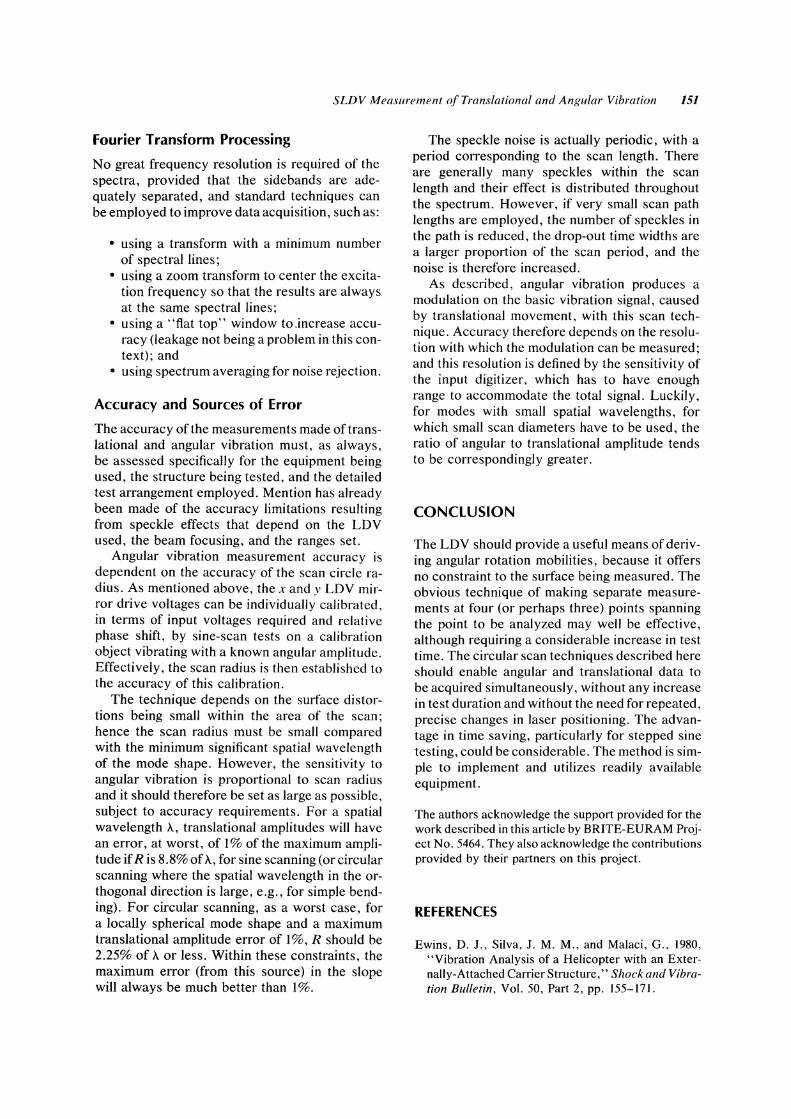
Figure 11 illustrates a short section of LDV and multiplier output signals recorded during this testing. Figure 12(a) shows the normal mobility FRF, referenced to the input force signal. With such narrow-band excitation only the central marked region is meaningful, but it contains more than sufficient data for modal analysis of the resonant mode. This analysis was carried out using ICATS MODENT software (Imregun, 1993), the curve fit being illustrated by comparing the fitted data to the Nyquist plot of the resonance.

As is common when testing a lightly damped structure, some mobility points near the peak were erroneous because of a low forcing input; they were removed from the Nyquist diagrams. The mobility modal constant derived from the Fig. 12(a) response was -0.152 mm/sN at a phase angle of 810. It was expected that this would be purely imaginary; the deviation from 900 was due to phase shift in the LDV output filter.

Sideband FRFs were also obtained using the multipliedIv reference, the result being illustrated in Fig. 12(b). The only meaningful data in this case are in the two sideband ranges marked. Frequency-shifted resonant responses are clearly defined and are plotted separately in Nyquist diagrams that include curve fits, based on modal analysis, in the same way as in Fig. 12(a). Equation (3) and the explanation of the derivation of angular vibration amplitudes given, apply equally to the" modal constants" obtained by modal analysis of the frequency-shifted FRFs. The only modification required is that the modal constant magnitudes have to be multiplied by (w ± fl)lw because of the frequency shifting. The relations in Table 3 can then be used directly to derive principal angular modal constants, in magnitude and phase, as well as to locate the principal rotation axes.

FREQUENCY Hz 250

FIGURE 9 LDV output spectrum, circular scan.


y

(a) I ti l~X

FIGURE 10

The two sidebands give modal constants of similar magnitude, which is to be expected in this case, where one principal angular modal constant is expected to be zero (i.e., 0.264 and 0.257 mml sN at phase angles of 98° and 66°, respectively). The angular modal constant is given, using Table 3, as 0.00362 rad/sN at 82°. The angle 'Y is given, using a value of 8 of -19°, as - 3°. Bearing in mind the experimental setup, angular and translational mobility modal constants are expected to have the same phase, 90°, and'Y should be 0°.

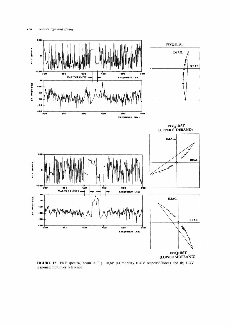
The beam was next rearranged to be inclined at 30°, as sketched in Fig. 9(b), and the test repeated. FRF data for this are shown in Fig. 13, equivalent to those in Fig. 12. The alignment of the sideband Nyquist plots is markedly different; sideband modal constants were 0.284 and 0.289 mm/sN at phase angles 127° and 38°. Application ofthe Table 3 formulae gave a translational modal constant of -0.162 mm/sN at 82° and an angular rotation model constant of 0.00399 rad/sN at 82°, with 'Y = 26°; the only difference in result to be expected is that the angle 'Y should now be 30°. Differences from expectation are small enough to give reasonable validation of the method.

MULTIPUER

REFERENCE

o

(b)

Test beam.

DISCUSSION

Speckle Interference Effects One problem in using LDVs is that, operating as they do with coherent light returned from diffusing surfaces, speckle effects produce regions where returned light is extinguished by destructive interference. The size of these areas can be minimized by proper focusing of the illuminating beam, and for quasistationary measurement this is not a serious problem. However, when scanning, the laser inevitably passes through the speckle pattern, giving multiple signal drop-outs. Figure 5 compares the forcing and LDV response signals associated with Figs. 3 and 4. In this case the LDV signal was small and the drop-outs are very noticeable. Nevertheless, as evident from Fig. 3, the averaging effect of FFT processing spreads such noise effects over the response spectrum to give, even in this case, quite a tolerable signal/noise ratio.

When carrying out the narrow-band resonance tests described above, LDV signals approached full scale more closely, and the drop-outs were far less severe, as shown in Fig. 11.

sees 0.0595

FIGURE 11 LDV and reference signals.

p H A S E , 0 (

" 0 D U L U S

d B

p H A s E

) 0 (

" 0 D U L U S

d B

2U1i1

II

-3ti1l1

II

-16

-33

-48

-64

-8ti1

288

II

-3ea 3ti1ti1

311

18

-111

-3ti1

-511

-"ltil 3_ 358 481i1


FREQUDlCII (Hz'

:I" :1:111

FREQUEI'ICII (Hz)

458 581i1 558

FRBQUEl'!CII (HII'

NYQUIST

IMAG.

l Ii

REAL

..

NYQUIST (UPPER SIDEBAND)

IMAG.

REAL

REAL

NYQUIST (LOWER SIDEBAND)

FIGURE 12 FRF spectra, beam in Fig. lO(a): (a) mobility (LDV response/force) and (b) LDV response/multiplier reference.

150 Stanhridge and Ewins

P H A S E

) o (

M o D U L U s d B

P H A S E

) o (

M o D U L U S

d B

299,-----------------------------------------------------,

-288+---------~--------~----;_~--+_--------~--------~ 31111 3511 4118 5l1li 5511

VAUDRANGE FREQUDlCII (Hz)

9,-------------------------;_~----------------------_,

-16

-32

-48

-64

-88+---------~--------_;----------+_--------;_--------~ 3BB 359 488 45B 58B 55B

FREQUDlCII (Hz)

29B,-------------------------------____________________ __,

111

-2111111+---------~--------_4~~----~+4--------4---------~ 3B9 358

VAUDRANGES 5B8 558

FREQUDlCII (Hz) 3111,---------------------t-~--._~_4------------------__,

1111

-18

-3111

-5111

-78+---------~--------_;----------+_--------;_----------i 388 35111 4111111 45111 588 558

FREQUEttCII (Hz)

NYQUIST

REAL

NYQUIST (UPPER SIDEBAND)

IMAG.

/ REAL

IMAG.

NYQUIST (LOWER SIDEBAND)

FIGURE 13 FRF spectra, beam in Fig. lOeb): (a) mobility (LDV response/force) and (b) LDV response/multiplier reference.


Fourier Transform Processing

No great frequency resolution is required of the spectra, provided that the sidebands are adequately separated, and standard techniques can be employed to improve data acquisition, such as:

• using a transform with a minimum number of spectral lines;

• using a zoom transform to center the excitation frequency so that the results are always at the same spectral lines;

• using a "flat top" window tojncrease accuracy (leakage not being a problem in this context); and

• using spectrum averaging for noise rejection.

Accuracy and Sources of Error

The accuracy of the measurements made of translational and angular vibration must, as always, be assessed specifically for the equipment being used, the structure being tested, and the detailed test arrangement employed. Mention has already been made of the accuracy limitations resulting from speckle effects that depend on the LOV used, the beam focusing, and the ranges set.

Angular vibration measurement accuracy is dependent on the accuracy of the scan circle radius. As mentioned above, the x and y LOV mirror drive voltages can be individually calibrated, in terms of input voltages required and relative phase shift, by sine-scan tests on a calibration object vibrating with a known angular amplitude. Effectively, the scan radius is then established to the accuracy of this calibration.

The technique depends on the surface distortions being small within the area of the scan; hence the scan radius must be small compared with the minimum significant spatial wavelength of the mode shape. However, the sensitivity to angular vibration is proportional to scan radius and it should therefore be set as large as possible, subject to accuracy requirements. For a spatial wavelength A, translational amplitudes will have an error, at worst, of 1 % of the maximum amplitude if R is 8.8% of A, for sine scanning (or circular scanning where the spatial wavelength in the orthogonal direction is large, e.g., for simple bending). For circular scanning, as a worst case, for a locally spherical mode shape and a maximum translational amplitude error of 1 %, R should be 2.25% of A or less. Within these constraints, the maximum error (from this source) in the slope will always be much better than 1 %.

The speckle noise is actually periodic, with a period corresponding to the scan length. There are generally many speckles within the scan length and their effect is distributed throughout the spectrum. However, if very small scan path lengths are employed, the number of speckles in the path is reduced, the drop-out time widths are a larger proportion of the scan period, and the noise is therefore increased.

As described, angular vibration produces a modulation on the basic vibration signal, caused by translational movement, with this scan technique. Accuracy therefore depends on the resolution with which the modulation can be measured; and this resolution is defined by the sensitivity of the input digitizer, which has to have enough range to accommodate the total signal. Luckily, for modes with small spatial wavelengths, for which small scan diameters have to be used, the ratio of angular to translational amplitude tends to be correspondingly greater.

CONCLUSION

The LOV should provide a useful means of deriving angular rotation mobilities, because it offers no constraint to the surface being measured. The obvious technique of making separate measurements at four (or perhaps three) points spanning the point to be analyzed may well be effective, although requiring a considerable increase in test time. The circular scan techniques described here should enable angular and translational data to be acquired simultaneously, without any increase in test duration and without the need for repeated, precise changes in laser positioning. The advantage in time saving, particularly for stepped sine testing, could be considerable. The method is simple to implement and utilizes readily available equipment.

The authors acknowledge the support provided for the work described in this article by BRITE-EURAM Project No. 5464. They also acknowledge the contributions provided by their partners on this project.

REFERENCES

Ewins, D. J., Silva, J. M. M., and Malaci, G., 1980, "Vibration Analysis of a Helicopter with an Externally-Attached Carrier Structure," Shock and Vibration Bulletin, Vol. 50, Part 2, pp. 155-17l.


Imregun, M., 1993, User's Guide to MODENT, Version 3.9A, ICATS, Imperial College, Dept. of Mechanical Engineering, London.

Sommer,H. J. III, Erickson, M. J., Trethewey, M. W., and Cafeo, J. A., 1994, "Single-Beam Laser Vibrometerfor Simultaneous Measurement of Translational, Pitch and Roll with Neural Network Calibration," in Proceedings of the 12th International Modal Analysis Conference, Vol. II, Honolulu, HI, pp. 1196-1201.

Uregueira, A. P. V., and Ewins, D. J., 1989, "A Refined Modal Coupling Technique for Including Residual Effects of Out-of-Range Modes," in Proceedings of the 7th International Modal Analysis Conference, Vol. I, Las Vegas, pp. 299-306.

Visser, W. J., Imregun, M., and Ewins, D. J., 1992, "Direct Use of Measured FRFData to Update Finite Element Models," in Proceedings of the 17th Internal Seminar on Modal Analysis, Vol. 1, Leuven, Belgium, pp. 33-49.

International Journal of

AerospaceEngineeringHindawi Publishing Corporationhttp://www.hindawi.com Volume 2010

RoboticsJournal of

Hindawi Publishing Corporationhttp://www.hindawi.com Volume 2014


Active and Passive Electronic Components

Control Scienceand Engineering

Journal of



RotatingMachinery


Hindawi Publishing Corporation http://www.hindawi.com

Journal ofEngineeringVolume 2014

Submit your manuscripts athttp://www.hindawi.com

VLSI Design



Shock and Vibration


Civil EngineeringAdvances in

Acoustics and VibrationAdvances in



Electrical and Computer Engineering

Journal of

Advances inOptoElectronics

Hindawi Publishing Corporation http://www.hindawi.com

Volume 2014

The Scientific World JournalHindawi Publishing Corporation http://www.hindawi.com Volume 2014

SensorsJournal of


Modelling & Simulation in EngineeringHindawi Publishing Corporation http://www.hindawi.com Volume 2014


Chemical EngineeringInternational Journal of Antennas and

Propagation




Navigation and Observation



DistributedSensor Networks


Documents

A. B. D. J. Ewins Measurement of Translational and …downloads.hindawi.com/journals/sv/1996/737569.pdf · and Angular Vibration ... two principal angular vibrations ... Processes