Embed Size (px)
Citation preview

Hindawi Publishing CorporationJournal of Inequalities and ApplicationsVolume 2009, Article ID 785628, 27 pagesdoi:10.1155/2009/785628
Research ArticleExistence and Stability ofSolutions for Nonautonomous StochasticFunctional Evolution Equations
Xianlong Fu
Department of Mathematics, East China Normal University, Shanghai 200241, China
Correspondence should be addressed to Xianlong Fu, [email protected]
Received 19 March 2009; Accepted 2 June 2009
Recommended by Jozef Banas
We establish the results on existence and exponent stability of solutions for a semilinearnonautonomous neutral stochastic evolution equation with finite delay; the linear part of thisequation is dependent on time and generates a linear evolution system. The obtained results areapplied to some neutral stochastic partial differential equations. These kinds of equations arisein systems related to couple oscillators in a noisy environment or in viscoelastic materials underrandom or stochastic influences.
Copyright q 2009 Xianlong Fu. This is an open access article distributed under the CreativeCommons Attribution License, which permits unrestricted use, distribution, and reproduction inany medium, provided the original work is properly cited.
1. Introduction
In this paper we study the existence and asymptotic behavior of mild solutions for thefollowing neutral non-autonomous stochastic evolution equation with finite delay:
d(Z(t) − k(t, Zt)) = [−A(t)(Z(t) − k(t, Zt)) + F(t, Zt)]dt +G(t, Zt)dW(t), 0 ≤ t ≤ T,Z0 = φ ∈ Lp(Ω, Cα),
(1.1)
where A(t) generates a linear evolution system, or say linear evolution operator {U(t, s) :0 ≤ s ≤ t ≤ T} on a separable Hilbert spaceH with the inner product (·, ·) and norm ‖ · ‖. k; Fand G are given functions to be specified later.
In recent years, existence, uniqueness, stability, invariant measures, and otherquantitative and qualitative properties of solutions to stochastic partial differential equationshave been extensively investigated by many authors. One of the important techniques to

2 Journal of Inequalities and Applications
discuss these topics is the semigroup approach; see, for example, Da Prato and Zabczyk [1],Dawson [2], Ichikawa [3], and Kotelenez [4]. In paper [5] Taniguchi et al. have investigatedthe existence and asymptotic behavior of solutions for the following stochastic functionaldifferential equation:
dZ(t) =[−AZ(t) + f(t, Zt)
]dt + g(t, Zt)dW(t), 0 ≤ t ≤ T,
Z0 = φ ∈ Lp(Ω, Cα),(1.2)
by using analytic semigroups approach and fractional power operator arguments. In thiswork as well as other related literatures like [6–9], the linear part of the discussedequation is an operator independent of time t and generates a strongly continuous (one-parameter) semigroup or analytic semigroup so that the semigroup approach can beemployed. We would also like to mention that some similar topics to the above for stochasticordinary functional differential equations with finite delays have already been investigatedsuccessfully by various authors (cf. [6, 10–13] and references in [14] among others). Relatedwork on functional stochastic evolution equations of McKean-Vlasov type and of second-order are discussed in [15, 16].
However, it occurs very often that the linear part of (1.2) is dependent on timet. Indeed, a lot of stochastic partial functional differential equations can be rewritten tosemilinear non-autonomous equations having the form of (1.2) with A = A(t). There existsmuch work on existence, asymptotic behavior, and controllability for deterministic non-autonomous partial (functional) differential equations with finite or infinite delays; see,for example, [17–20]. But little is known to us for non-autonomous stochastic differentialequations in abstract space, especially for the case that A(t) is a family of unboundedoperators.
Our purpose in the present paper is to obtain results concerning existence, uniqueness,and stability of the solutions of the non-autonomous stochastic differential equations (1.1). Amotivation example for this class of equations is the following non-autonomous boundaryproblem:
d(Z(t, x) − bZ(t − r, x)) =[
a(t, x)∂2
∂2x(Z(t, x) − bZ(t − r, x)) + f(t, Z(t + r1(t), x))
]
dt
+ g(t, Z(t + r1(t), x))dβ(t),
Z(t, 0) = Z(t, π) = 0, t ≥ 0,
Z(θ, x) = φ(x), θ ∈ [−r, 0], 0 ≤ x ≤ π.
(1.3)
As stated in paper [21], these problems arise in systems related to couple oscillators in a noisyenvironment or in viscoelastic materials under random or stochastic influences (see also [22]for the discussion for the corresponding determined systems). Therefore, it is meaningful todeal with (1.1) to acquire some results applicable to problem (1.3). In paper [21], Caraballo

Journal of Inequalities and Applications 3
et al. have, under coercivity condition in an integral form, investigated the second moment(almost sure) exponential stability and ultimate boundedness of solutions to the followingnon-autonomous semilinear stochastic delay equation:
d(X(t) − k(t, X(t − r))) = [A(t)X(t) + F(t, Xt)]dt +G(t, Xt)dW(t), t ≥ 0,
X(t) = φ(t) t ∈ [−r, 0](1.4)
on a Hilbert spaceH, where A(·) ∈ L∞(0, T ;L(V, V ∗))with V ⊂ H ⊂ H∗ ⊂ V ∗.As we know, non-autonomous evolution equations are much more complicate than
autonomous ones to be dealt with. Our approach here is inspired by the work in paper[5, 18, 19]. That is, we assume that {A(t) : t ≥ 0} is a family of unbounded linear operators onH with (common) dense domain such that it generates a linear evolution system. Thus wewill apply the theory of linear evolution system and fractional power operators methodsto discuss existence, uniqueness, and pth (p > 2) moment exponential stability of mildsolutions to the stochastic partial functional differential equation (1.1). Clearly our workcan be regarded as extension and development of that in [5, 21] and other related papersmentioned above.
We will firstly in Section 2 introduce some notations, concepts, and basic resultsabout linear evolution system and stochastic process. The existence and uniqueness of mildsolutions are discussed in Section 3 by using Banach fixed point theorem. In Section 4, weinvestigate the exponential stability for the mild solutions obtained in Section 3, and theconditions for stability are somewhat weaker than in [5]. Finally, in Section 5 we apply theobtained results to (1.3) to illustrate the applications.
2. Preliminaries
In this section we collect some notions, conceptions, and lemmas on stochastic process andlinear evolution system which will be used throughout the whole paper.
Let (Ω,F, P) be a probability space on which an increasing and right continuousfamily {Ft}t∈[0,+∞) of complete sub-σ-algebras of F is defined. H and K are two separableHilbert space. Suppose that W(t) is a given K-valued Wiener Process with a finite tracenuclear covariance operator Q > 0. Let βn(t), n = 1, 2, . . ., be a sequence of real-valued one-dimensional standard Brownian motions mutually independent over (Ω,F, P). Set
W(t) =+∞∑
n=1
√λnβn(t)en, t ≥ 0, (2.1)
where λn ≥ 0 (n = 1, 2, . . .) are nonnegative real numbers, and {en} (n = 1, 2, . . .) is a completeorthonormal basis in K. Let Q ∈ L(K,K) be an operator defined by Qen = λnen with finitetrace trQ =
∑+∞n=1 λn < ∞. Then the above K-valued stochastic process W(t) is called a Q-
Wiener process.
4 Journal of Inequalities and Applications
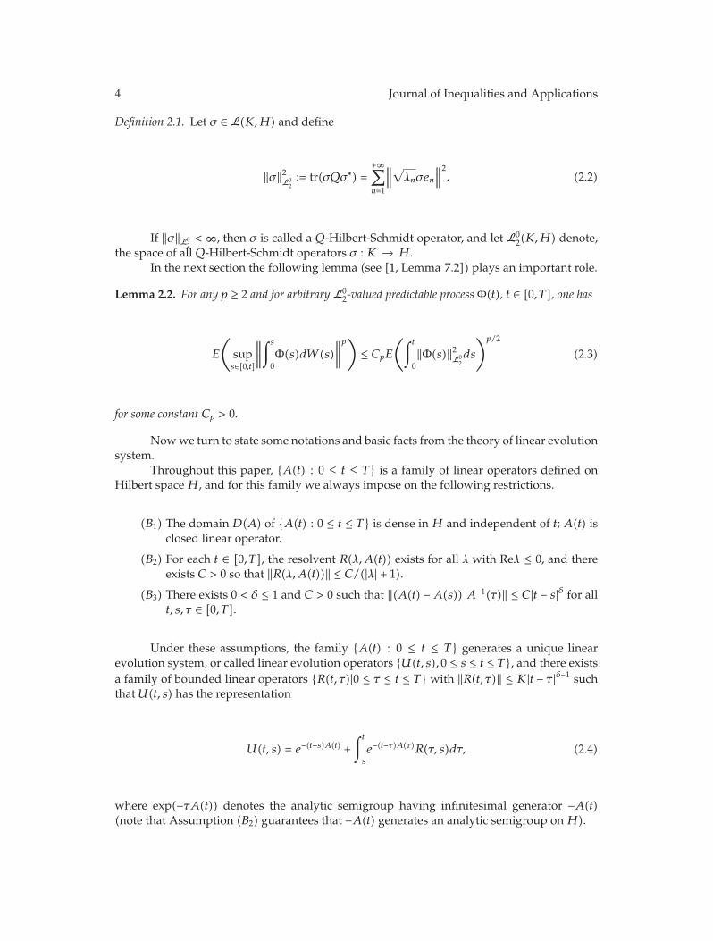
Definition 2.1. Let σ ∈ L(K,H) and define
‖σ‖2L02:= tr(σQσ∗) =
+∞∑
n=1
∥∥∥√λnσen
∥∥∥2. (2.2)
If ‖σ‖L02< ∞, then σ is called a Q-Hilbert-Schmidt operator, and let L0
2(K,H) denote,the space of all Q-Hilbert-Schmidt operators σ : K → H.
In the next section the following lemma (see [1, Lemma 7.2]) plays an important role.
Lemma 2.2. For any p ≥ 2 and for arbitrary L02-valued predictable process Φ(t), t ∈ [0, T], one has
E
(
sups∈[0,t]
∥∥∥∥
∫ s
0Φ(s)dW(s)
∥∥∥∥
p)
≤ CpE
(∫ t
0‖Φ(s)‖2L0
2ds
)p/2
(2.3)
for some constant Cp > 0.
Nowwe turn to state some notations and basic facts from the theory of linear evolutionsystem.
Throughout this paper, {A(t) : 0 ≤ t ≤ T} is a family of linear operators defined onHilbert spaceH, and for this family we always impose on the following restrictions.
(B1) The domain D(A) of {A(t) : 0 ≤ t ≤ T} is dense inH and independent of t; A(t) isclosed linear operator.
(B2) For each t ∈ [0, T], the resolvent R(λ,A(t)) exists for all λ with Reλ ≤ 0, and thereexists C > 0 so that ‖R(λ,A(t))‖ ≤ C/(|λ| + 1).
(B3) There exists 0 < δ ≤ 1 and C > 0 such that ‖(A(t) −A(s)) A−1(τ)‖ ≤ C|t − s|δ for allt, s, τ ∈ [0, T].
Under these assumptions, the family {A(t) : 0 ≤ t ≤ T} generates a unique linearevolution system, or called linear evolution operators {U(t, s), 0 ≤ s ≤ t ≤ T}, and there existsa family of bounded linear operators {R(t, τ)|0 ≤ τ ≤ t ≤ T} with ‖R(t, τ)‖ ≤ K|t − τ |δ−1 suchthatU(t, s) has the representation
U(t, s) = e−(t−s)A(t) +∫ t
s
e−(t−τ)A(τ)R(τ, s)dτ, (2.4)
where exp(−τA(t)) denotes the analytic semigroup having infinitesimal generator −A(t)(note that Assumption (B2) guarantees that −A(t) generates an analytic semigroup onH).

Journal of Inequalities and Applications 5
For the linear evolution system {U(t, s), 0 ≤ s ≤ t ≤ T}, the following properties arewell known:
(a) U(t, s) ∈ L(H), the space of bounded linear transformations on H, whenever 0 ≤s ≤ t ≤ T and maps H into D(A) as t > s. For each x ∈ H, the mapping (t, s) →U(t, s)x is continuous jointly in s and t;
(b) U(t, s)U(s, τ) = U(t, τ) for 0 ≤ τ ≤ s ≤ t ≤ T ;(c) U(t, t) = I;
(d) (∂/∂t)U(t, s) = −A(t)U(t, s), for s < t.
We also have the following inequalities:
∥∥∥e−tA(s)∥∥∥ ≤ K, t ≥ 0, s ∈ [0, T],
∥∥∥A(s)e−tA(s)∥∥∥ ≤ K
t, t, s ∈ [0, T],
‖A(t)U(t, s)‖ ≤ K
|t − s| , 0 ≤ s ≤ t ≤ T.
(2.5)
Furthermore, Assumptions (B1)–(B3) imply that for each t ∈ [0, T] the integral
A−α(t) =1
Γ(α)
∫+∞
0sα−1e−sA(t)ds (2.6)
exists for each α ∈ (0, 1]. The operator defined by (2.6) is a bounded linear operator andyields A−α(t)A−β(t) = A−(α+β)(t). Thus, we can define the fractional power as
Aα(t) =[A−α(t)
]−1, (2.7)
which is a closed linear operator with D(Aα(t)) dense in H and D(Aα(t)) ⊂ D(Aβ(t)) forα ≥ β. D(Aα(t)) becomes a Banach space endowed with the norm ‖x‖α,t = ‖Aα(t)x‖, which isdenoted byHα(t).
The following estimates and Lemma 2.3 are from ([23, Part II]):
∥∥∥Aα(t)A−β(τ)∥∥∥ ≤ K(
α, β)
(2.8)
6 Journal of Inequalities and Applications
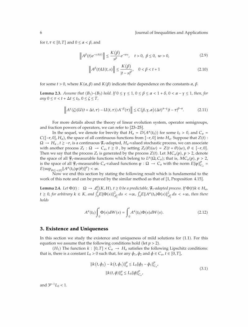
for t, τ ∈ [0, T] and 0 ≤ α < β, and
∥∥∥Aβ(t)e−sA(t)∥∥∥ ≤ K
(β)
sβe−ws, t > 0, β ≤ 0, w > 0, (2.9)
∥∥∥Aβ(t)U(t, s)∥∥∥ ≤ K
(β)
|t − s|β, 0 < β < t + 1 (2.10)
for some t > 0, where K(α, β) and K(β) indicate their dependence on the constants α, β.
Lemma 2.3. Assume that (B1)–(B3) hold. If 0 ≤ γ ≤ 1, 0 ≤ β ≤ α < 1 + δ, 0 < α − γ ≤ 1, then, forany 0 ≤ τ < t + Δt ≤ t0, 0 ≤ ζ ≤ T ,
∥∥∥Aγ(ζ)(U(t + Δt, τ) −U(t, τ))A−β(τ)∥∥∥ ≤ C(β, γ, α)(Δt)α−γ |t − τ |β−α. (2.11)
For more details about the theory of linear evolution system, operator semigroups,and fraction powers of operators, we can refer to [23–25].
In the sequel, we denote for brevity that Hα = D(Aα(t0)) for some t0 > 0, and Cα =C([−r, 0],Hα), the space of all continuous functions from [−r, 0] intoHα. Suppose that Z(t) :Ω → Hα , t ≥ −r, is a continuous Ft-adapted,Hα-valued stochastic process, we can associatewith another process Zt : Ω → Cα, t ≥ 0 , by setting Zt(θ)(ω) = Z(t + θ)(ω), θ ∈ [−r, 0].Then we say that the process Zt is generated by the process Z(t). LetMCα(p), p > 2, denotethe space of all Ft-measurable functions which belong to Lp(Ω, Cα); that is, MCα(p), p > 2,is the space of all Ft-measurable Cα-valued functions ψ : Ω → Cα with the norm E‖ψ‖pCα
=E(supθ∈[−r,0]‖Aα(t0)ψ(θ)‖p) <∞.
Now we end this section by stating the following result which is fundamental to thework of this note and can be proved by the similar method as that of [1, Proposition 4.15].
Lemma 2.4. LetΦ(t) : Ω → L02(K,H), t ≥ 0 be a predictable, Ft-adapted process. IfΦ(t)k ∈ Hα,
t ≥ 0, for arbitrary k ∈ K, and∫ t0E‖Φ(s)‖2L0
2ds < +∞,
∫ t0E‖Aα(t0)Φ(s)‖2L0
2ds < +∞, then there
holds
Aα(t0)∫ t
0Φ(s)dW(s) =
∫ t
0Aα(t0)Φ(s)dW(s). (2.12)
3. Existence and Uniqueness
In this section we study the existence and uniqueness of mild solutions for (1.1). For thisequation we assume that the following conditions hold (let p > 2).
(H1) The function k : [0, T] × Cα → Hα satisfies the following Lipschitz conditions:that is, there is a constant L0 > 0 such that, for any φ1, φ2 and φ ∈ Cα, t ∈ [0, T],
‖k(t, φ2) − k(t, φ1
)‖pα ≤ L0‖φ2 − φ1‖pCα,
‖k(t, φ)‖pα ≤ L0‖φ‖pCα,
(3.1)
and 3p−1L0 < 1.
Journal of Inequalities and Applications 7
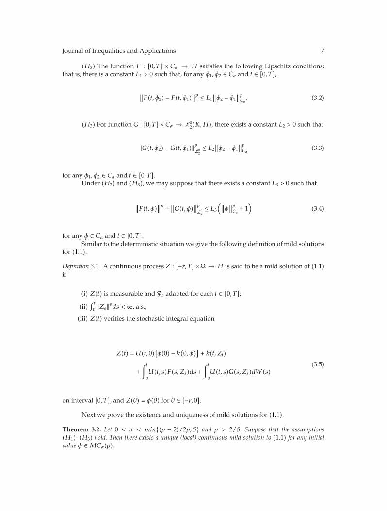
(H2) The function F : [0, T] × Cα → H satisfies the following Lipschitz conditions:that is, there is a constant L1 > 0 such that, for any φ1, φ2 ∈ Cα and t ∈ [0, T],
∥∥F(t, φ2) − F(t, φ1)∥∥p ≤ L1
∥∥φ2 − φ1∥∥pCα. (3.2)
(H3) For function G : [0, T] × Cα → L02(K,H), there exists a constant L2 > 0 such that
‖G(t, φ2) −G(t, φ1)‖pL02≤ L2
∥∥φ2 − φ1∥∥pCα
(3.3)
for any φ1, φ2 ∈ Cα and t ∈ [0, T].Under (H2) and (H3), we may suppose that there exists a constant L3 > 0 such that
∥∥F(t, φ)∥∥p +
∥∥G(t, φ)∥∥pL0
2≤ L3
(∥∥φ∥∥pCα
+ 1)
(3.4)
for any φ ∈ Cα and t ∈ [0, T].Similar to the deterministic situation we give the following definition of mild solutions
for (1.1).
Definition 3.1. A continuous process Z : [−r, T]×Ω → H is said to be a mild solution of (1.1)if
(i) Z(t) is measurable and Ft-adapted for each t ∈ [0, T];
(ii)∫T0 ‖Zs‖pds <∞, a.s.;
(iii) Z(t) verifies the stochastic integral equation
Z(t) = U(t, 0)[φ(0) − k(0, φ)] + k(t, Zt)
+∫ t
0U(t, s)F(s, Zs)ds +
∫ t
0U(t, s)G(s, Zs)dW(s)
(3.5)
on interval [0, T], and Z(θ) = φ(θ) for θ ∈ [−r, 0].
Next we prove the existence and uniqueness of mild solutions for (1.1).
Theorem 3.2. Let 0 < α < min{(p − 2)/2p, δ} and p > 2/δ. Suppose that the assumptions(H1)–(H3) hold. Then there exists a unique (local) continuous mild solution to (1.1) for any initialvalue φ ∈MCα(p).

8 Journal of Inequalities and Applications
Proof. Denote byD the Banach space of all the continuous processes Z(t)which belong to thespace C([−r, T], Lp(Ω,H)) with ‖Z‖D <∞, where
‖Z‖D := supt∈[0,T]
(E‖Zt‖pC
)1/p,
E‖Zt‖pC := E
(
supθ∈[−r,0]
‖Zt(θ)‖p)
.
(3.6)
Define the operator Ψ on D:
(ΨZ)(t) = Aα(t0)U(t, 0)[φ(0) − k(0, φ)] +Aα(t0)k
(t, A−α(t0)Zt
)
+∫ t
0Aα(t0)U(t, s)F
(s,A−α(t0)Zs
)ds +
∫ t
0Aα(t0)U(t, s)G
(s,A−α(t0)Zs
)dW(s).
(3.7)
Then it is clear that to prove the existence of mild solutions to (1.1) is equivalent to find afixed point for the operator Ψ. Next we will show by using Banach fixed point theorem thatΨ has a unique fixed point. We divide the subsequent proof into three steps.
Step 1. For arbitrary Z ∈ D, (ΨZ)(t) is continuous on the interval [0, T] in the Lp-sense.Let 0 < t < T and |h| be sufficiently small. Then for any fixed Z ∈ D, we have that
E‖(ΨZ)(t + h) − (ΨZ)(t)‖p ≤ 4p−1E∥∥Aα(t0)(U(t + h, 0) −U(t, 0))
[φ(0) − k(0, φ)]∥∥p
+ 4p−1E‖Aα(t0)[k(t + h,Aα(t0)Zt+h) − k(t, Aα(t0)Zt)]‖p
+ 4p−1E
∥∥∥∥∥
∫ t+h
0Aα(t0)U(t + h, s)F
(s,A−α(t0)Zs
)ds
−∫ t
0A−α(t0)U(t, s)F(s,A−α(t0)Zs)ds
∥∥∥∥∥
p
+ 4p−1E
∥∥∥∥∥
∫ t+h
0Aα(t0)U(t + h, s)G
(s,A−α(t0)Zs
)dW(s)
−∫ t
0Aα(t0)U(t, s)G(s,A−α(t0)Zs)dW(s)
∥∥∥∥∥
p
:= I1 + I2 + I3 + I4.
(3.8)
Thus, by Lemma 2.3 we get
I1 = 4p−1E‖Aα(t0)(U(t + h, 0) −U(t, 0))A−β(t0)Aβ(t0)[φ(0) − k(0, φ)]‖p
≤ 4p−1Cp|h|p(β−α)E‖Aβ(t0)[φ(0) − k(0, φ)]‖p,(3.9)

Journal of Inequalities and Applications 9
where β > 0 satisfies that α < β < 1 and C > 0 are constant. From Condition (H2) it followsthat
I3 ≤ 8p−1E
∥∥∥∥∥
∫ t
0Aα(t0)[U(t + h, s) −U(t, s)]F(s,A−α(t0)Zs)ds
∥∥∥∥∥
p
+ 8p−1E
∥∥∥∥∥
∫ t+h
t
Aα(t0)U(t + h, s)F(s,A−α(t0)Zs
)ds
∥∥∥∥∥
p
= I31 + I32.
(3.10)
And by (2.8)–(2.10) one has that
I32 ≤ 8p−1E
(∫ t+h
t
‖Aα(t0)A−β(t + h)‖‖Aβ(t + h)U(t + h, s)‖‖F(s,A−α(t0)Zs
)‖ds)p
≤ 8p−1(K(α, β
)K(β))p
E
(∫ t+h
t
1
(t + h − s)β∥∥F
(s,A−α(t0)Zs
)∥∥ds
)p
≤ 8p−1(K(α, β
)K(β))p
(∫ t+h
t
1
(t + h − s)qβds
)p/q
E
∫ t+h
t
‖F(s,A−α(t0)Zs
)‖pds
≤ 8p−1(K(α, β
)K(β))p
(1
1 − qβ)p−1
L3h(1−β)p(1 + ‖Z‖pD
),
(3.11)
where q > 0 solves 1/p + 1/q = 1, and
I31 = 8p−1E
∥∥∥∥∥
∫ t
0Aα(t0)
[
e−(t+h−s)A(t+h) +∫ t+h
s
e−(t+h−τ)A(τ)R(τ, s)dτ
−e−(t−s)A(t) −∫ t
s
e−(t−τ)A(τ)R(τ, s)dτ
]
F(s,A−α(t0)Zs)ds
∥∥∥∥∥
p
≤ 8p−1⎛
⎝∫ t
0
∥∥∥∥∥∥Aα(t0)
⎡
⎣e−(t+h−s)A(t+h)
+∫ t+h
s
e−(t+h−τ)A(τ)R(τ, s)dτ
−e−(t−s)A(t) −∫ t
s
e−(t−τ)A(τ)R(τ, s)dτ
]∥∥∥∥∥
q
ds
⎞
⎠
p/q
× E(∫ t
0
∥∥F(s,A−α(t0)Zs
)∥∥pds
)
:= 8p−1I ′p/q31 E
(∫ t
0‖F(s,A−α(t0)Zs
)‖pds)
≤ 8p−1L3I′p/q31 T(1 + ‖Z‖pD
),
(3.12)
10 Journal of Inequalities and Applications
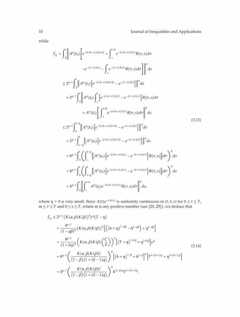
while
I ′31 =∫ t
0
∥∥∥∥∥Aα(t0)
[
e−(t+h−s)A(t+h) +∫ t+h
s
e−(t+h−τ)A(τ)R(τ, s)dτ
−e−(t−s)A(t) −∫ t
s
e−(t−τ)A(τ)R(τ, s)dτ
]∥∥∥∥∥
q
ds
≤ 2q−1∫ t
0
∥∥∥Aα(t0)[e−(t+h−s)A(t+h) − e−(t−s)A(t)
]∥∥∥qds
+ 2q−1∫ t
0
∥∥∥∥∥Aα(t0)
∫ t
s
[e−(t+h−τ)A(τ) − e−(t−τ)A(τ)
]R(τ, s)dτ
+Aα(t0)
[ ∫ t+h
t
e−(t+h−τ)A(τ)R(τ, s)dτ
∥∥∥∥∥
q
ds
≤ 2q−1∫ t−η
0
∥∥∥Aα(t0)[e−(t+h−s)A(t+h) − e−(t−s)A(t)
]∥∥∥qds
+ 2q−1∫ t
t−η
∥∥∥Aα(t0)[e−(t+h−s)A(t+h) − e−(t−s)A(t)
]∥∥∥qds
+ 8q−1∫ t
0
(∫ t−η
s
∥∥∥Aα(t0)[e−(t+h−τ)A(τ) − e−(t−τ)A(τ)
]R(τ, s)
∥∥∥dτ
)q
ds
+ 8q−1∫ t
0
(∫ t
t−η
∥∥∥Aα(t0)[e−(t+h−τ)A(τ) − e−(t−τ)A(τ)
]R(τ, s)
∥∥∥dτ
)q
ds
+ 4q−1∫ t
0
∥∥∥∥∥
∫ t+h
t
Aα(t0)e−(t+h−τ)A(τ)R(τ, s)dτ
∥∥∥∥∥
q
ds,
(3.13)
where η > 0 is very small. Since A(t)e−τA(s) is uniformly continuous in (t, τ, s) for 0 ≤ t ≤ T ,m ≤ τ ≤ T and 0 ≤ s ≤ T , wherem is any positive number (see [23, 25]), we deduce that
I ′31 ≤ 2q−1(K(α, β)K(β)
)qεq(T − η)
+4q−1
(1 − qβ)q(K(α, β)K(β)
)q[((h + η
)1−qβ − h1−qβ)+ η1−qβ
]
+8q−1
(1 + δq)q
(K(α, β)K(β)
(C
δ
))q[(T + η
)1+δq + η1+δq]εq
+ 8q−1(
K(α, β)K(β)C(1 − β)(1 + (δ − 1)q
)
)q[(h + η
)1−β + h1−β]q[
T1+(δ−1)q + η1+(δ−1)q]
+ 4q−1(
K(α, β)K(β)C(1 − β)(1 + (δ − 1)q
)
)q
h(1−β)qT1+(δ−1)q.
(3.14)
Journal of Inequalities and Applications 11
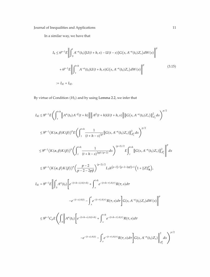
In a similar way, we have that
I4 ≤ 6p−1E
∥∥∥∥∥
∫ t
0A−α(t0)[U(t + h, s) −U(t − s)]G(s,A−α(t0)Zs
)dW(s)
∥∥∥∥∥
p
+ 6p−1E
∥∥∥∥∥
∫ t+h
t
A−α(t0)U(t + h, s)G(s,A−α(t0)Zs
)dW(s)
∥∥∥∥∥
p
:= I41 + I42.
(3.15)
By virtue of Condition (H3) and by using Lemma 2.2, we infer that
I42 ≤ 8p−1E
(∫ t+h
t
∥∥∥Aα(t0)A−β(t + h)∥∥∥∥∥∥Aβ(t + h)U(t + h, s)
∥∥∥∥∥G
(s,A−α(t0)Zs
)∥∥2L2ds
)p/2
≤ 8p−1(K(α, β)K(β)
)pE
(∫ t+h
t
1
(t + h − s)2β∥∥G(s,A−α(t0)Zs)
∥∥2L0
2ds
)p/2
≤ 8p−1(K(α, β)K(β)
)p(∫ t+h
t
1
(t + h − s)2pβ/(p−2)ds
)(p−2)/2E
∫ t+h
t
∥∥G(s,A−α(t0)Zs)∥∥2L0
2
∥∥∥∥∥∥
p
ds
≤ 8p−1(K(α, β
)K(β))p
(p − 2
p − 2 − 2pβ
)(p−2)/2L3h(p−2)/(p−2−2pβ)+1
(1 + ‖Z‖pD
),
I41 = 8p−1E
∥∥∥∥∥
∫ t
0Aα(t0)
[
e−(t+h−s)A(t+h) +∫ t+h
s
e−(t+h−τ)A(τ)R(τ, s)dτ
−e−(t−s)A(t) −∫ t
s
e−(t−τ)A(τ)R(τ, s)dτ
]
G(s,A−α(t0)Zs)dW(s)
∥∥∥∥∥
p
≤ 8p−1CpE
⎛
⎝∫ t
0
∥∥∥∥∥Aα(t0)
[
e−(t+h−s)A(t+h) +∫ t+h
s
e−(t+h−τ)A(τ)R(τ, s)dτ
−e−(t−s)A(t) −∫ t
s
e−(t−τ)A(τ)R(τ, s)dτ
]
G(s,A−α(t0)Zs)
∥∥∥∥∥
2
L02
ds
⎞
⎠
p/2
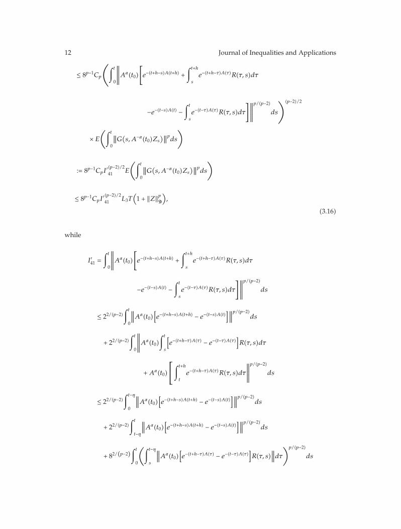
12 Journal of Inequalities and Applications
≤ 8p−1Cp
⎛
⎝∫ t
0
∥∥∥∥∥Aα(t0)
[
e−(t+h−s)A(t+h) +∫ t+h
s
e−(t+h−τ)A(τ)R(τ, s)dτ
−e−(t−s)A(t) −∫ t
s
e−(t−τ)A(τ)R(τ, s)dτ
]∥∥∥∥∥
p/(p−2)ds
⎞
⎠
(p−2)/2
× E(∫ t
0
∥∥G(s,A−α(t0)Zs
)∥∥pds
)
:= 8p−1CpI′(p−2)/241 E
(∫ t
0
∥∥G(s,A−α(t0)Zs
)∥∥pds
)
≤ 8p−1CpI′(p−2)/241 L3T
(1 + ‖Z‖pD
),
(3.16)
while
I ′41 =∫ t
0
∥∥∥∥∥Aα(t0)
[
e−(t+h−s)A(t+h) +∫ t+h
s
e−(t+h−τ)A(τ)R(τ, s)dτ
−e−(t−s)A(t) −∫ t
s
e−(t−τ)A(τ)R(τ, s)dτ
]∥∥∥∥∥
p/(p−2)ds
≤ 22/(p−2)∫ t
0
∥∥∥Aα(t0)[e−(t+h−s)A(t+h) − e−(t−s)A(t)
]∥∥∥p/(p−2)
ds
+ 22/(p−2)∫ t
0
∥∥∥∥∥Aα(t0)
∫ t
s
[e−(t+h−τ)A(τ) − e−(t−τ)A(τ)
]R(τ, s)dτ
+Aα(t0)
⎡
⎣∫ t+h
t
e−(t+h−τ)A(τ)R(τ, s)dτ
∥∥∥∥∥
p/(p−2)ds
≤ 22/(p−2)∫ t−η
0
∥∥∥Aα(t0)[e−(t+h−s)A(t+h) − e−(t−s)A(t)
]∥∥∥p/(p−2)
ds
+ 22/(p−2)∫ t
t−η
∥∥∥Aα(t0)[e−(t+h−s)A(t+h) − e−(t−s)A(t)
]∥∥∥p/(p−2)
ds
+ 82/(p−2)∫ t
0
(∫ t−η
s
∥∥∥Aα(t0)[e−(t+h−τ)A(τ) − e−(t−τ)A(τ)
]R(τ, s)
∥∥∥dτ
)p/(p−2)ds
Journal of Inequalities and Applications 13
+ 82/(p−2)∫ t
0
∥∥∥∥∥Aα(t0)
∫ t
t−η
[e−(t+h−τ)A(τ) − e−(t−τ)A(τ)
]R(τ, s)
∥∥∥∥∥dτ
)p/(p−2)ds
+ 42/(p−2)∫ t
0
∥∥∥∥∥
∫ t+h
t
Aα(t0)e−(t+h−τ)A(τ)R(τ, s)dτ
∥∥∥∥∥
p/(p−2)ds.
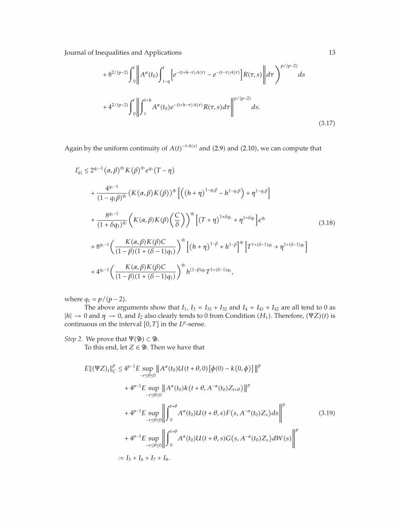
(3.17)
Again by the uniform continuity of A(t)−τA(s) and (2.9) and (2.10), we can compute that
I ′41 ≤ 2q1−1(α, β
)q1K(β)q1εq1
(T − η)
+4q1−1
(1 − q1β)q1(K(α, β
)K(β))q1
[((h + η
)1−q1β − h1−q1β)+ η1−q1β
]
+8q1−1
(1 + δq1)q1
(K(α, β)K(β)
(C
δ
))q1[(T + η
)1+δq1 + η1+δq1]εq1
+ 8q1−1(
K(α, β)K(β)C(1 − β)(1 + (δ − 1)q1)
)q1[(h + η
)1−β + h1−β]q1[
T1+(δ−1)q1 + η1+(δ−1)q1]
+ 4q1−1(
K(α, β)K(β)C(1 − β)(1 + (δ − 1)q1)
)q1
h(1−β)q1T1+(δ−1)q1 ,
(3.18)
where q1 = p/(p − 2).The above arguments show that I1, I3 = I31 + I32 and I4 = I41 + I42 are all tend to 0 as
|h| → 0 and η → 0, and I2 also clearly tends to 0 from Condition (H1). Therefore, (ΨZ)(t) iscontinuous on the interval [0, T] in the Lp-sense.
Step 2. We prove that Ψ(D) ⊂ D.To this end, let Z ∈ D. Then we have that
E‖(ΨZ)t‖pC ≤ 4p−1E sup−r≤θ≤0
∥∥Aα(t0)U(t + θ, 0)[φ(0) − k(0, φ)]∥∥p
+ 4p−1E sup−r≤θ≤0
∥∥Aα(t0)k(t + θ,A−α(t0)Zt+θ
)∥∥p
+ 4p−1E sup−r≤θ≤0
∥∥∥∥∥
∫ t+θ
0Aα(t0)U(t + θ, s)F
(s,A−α(t0)Zs
)ds
∥∥∥∥∥
p
+ 4p−1E sup−r≤θ≤0
∥∥∥∥∥
∫ t+θ
0Aα(t0)U(t + θ, s)G
(s,A−α(t0)Zs
)dW(s)
∥∥∥∥∥
p
:= I5 + I6 + I7 + I8.
(3.19)
14 Journal of Inequalities and Applications
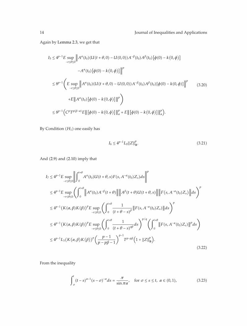
Again by Lemma 2.3, we get that
I5 ≤ 4p−1E sup−r≤θ≤0
∥∥∥Aα(t0)(U(t + θ, 0) −U(0, 0))A−β(t0)Aβ(t0)[φ(0) − k(0, φ)]
−Aα(t0)[φ(0) − k(0, φ)]
∥∥∥p
≤ 8p−1(
E sup−r≤θ≤0
∥∥∥Aα(t0)(U(t + θ, 0) −U(0, 0))A−β(t0)Aβ(t0)[φ(0) − k(0, φ)]∥∥∥p
+E∥∥Aα(t0)
[φ(0) − k(0, φ)]∥∥p
)
≤ 8p−1(CpTp(β−α)E
∥∥[φ(0) − k(0, φ)]∥∥pα + E∥∥[φ(0) − k(0, φ)]∥∥pα
).
(3.20)
By Condition (H1) one easily has
I6 ≤ 4p−1L0‖Z‖pD. (3.21)
And (2.9) and (2.10) imply that
I7 ≤ 4p−1E sup−r≤θ≤0
∥∥∥∥∥
∫ t+θ
0Aα(t0)U(t + θ, s)F(s,A−α(t0)Zs)ds
∥∥∥∥∥
p
≤ 4p−1E sup−r≤θ≤0
(∫ t+θ
0
∥∥∥Aα(t0)A−β(t + θ)∥∥∥∥∥∥Aβ(t + θ)U(t + θ, s)
∥∥∥∥∥∥F
(s,A−α(t0)Zs
)∥∥∥ds
)p
≤ 4p−1(K(α, β)K(β)
)pE sup−r≤θ≤0
(∫ t+θ
0
1
(t + θ − s)β∥∥F(s,A−α(t0)Zs)
∥∥ds
)p
≤ 4p−1(K(α, β)K(β)
)pE sup−r≤θ≤0
(∫ t+θ
0
1
(t + θ − s)qβds
)p/q(∫ t+θ
0
∥∥F(s,A−α(t0)Zs)∥∥pds
)
≤ 4p−1L3(K(α, β
)K(β))p
(p − 1
p − pβ − 1
)p−1Tp−pβ
(1 + ‖Z‖pD
).
(3.22)
From the inequality
∫ t
σ
(t − s)α−1(s − σ)−αds = π
sinπα, for σ ≤ s ≤ t, α ∈ (0, 1), (3.23)
Journal of Inequalities and Applications 15
established in [26], it follows that
I8 = 3p−1∣∣∣∣sinπγπ
∣∣∣∣
p
E sup−r≤θ≤0
∥∥∥∥∥
∫ t+θ
0Aα(t0)U(t + θ, s)(t + θ − s)γ−1R(s)ds
∥∥∥∥∥
p
,(3.24)
where
R(s) =∫s
0(s − σ)−γU(s, σ)G
(σ,A−α(t0)Zσ
)dW(σ), (3.25)
and 0 < γ < (p − 2)/2p. Thus,
I8 ≤ 3p−1(K(α, β)K(β)
∣∣∣∣sinπγπ
∣∣∣∣
)p
E sup−r≤θ≤0
∥∥∥∥∥
∫ t+θ
0(t + θ − s)γ−β−1R(s)ds
∥∥∥∥∥
p
≤ 3p−1L3Cp
(K(α, β)K(β)M0
)p(
p − 1p(β − γ) − 1
)p−1Tp(β−γ)−1
· 11 − 2pγ/
(p − 2
)T4−2pγ/(p−2)(1 + ‖Z‖pD
),
(3.26)
whereM0 = sup0≤σ≤s≤T‖U(s, σ)‖. Hence ‖ΨZ‖pD <∞ and so Ψ(D) ⊂ D.
Step 3. It remains to verify that Ψ is a contraction on D.Suppose that Z1, Z2 ∈ D, then for any fixed t ∈ [0, T],
E‖(ΨZ2)t − (ΨZ1)t‖pC
≤ 3p−1E sup−r≤θ≤0
∥∥Aα(t0)k(t + θ,A−α(t0)Z2,t+θ) −Aα(t0)k(t + θ,A−α(t0)Z1,t+θ
)∥∥p
+ 3p−1E sup−r≤θ≤0
∥∥∥∥∥
∫ t+θ
0Aα(t0)U(t + θ, s)
[F(s,A−α(t0)Z2(s)
) − F(s,A−α(t0)Z1(s))]ds
∥∥∥∥∥
p
+ 3p−1E sup−r≤θ≤0
∥∥∥∥∥
∫ t+θ
0Aα(t0)U(t + θ, s)
[G(s,A−α(t0)Z2(s)
) −G(s,A−α(t0)Z1(s))]dW(s)
∥∥∥∥∥
p
:= I9 + I10 + I11.(3.27)
16 Journal of Inequalities and Applications
Clearly,
I9 ≤ 3p−1L0‖Z2 − Z1‖pD,
I10 ≤(K(α, β)K(β)
)pE sup−r≤θ≤0
(∫ t+θ
0
1
(t + θ − s)qβds
)p/q
×(∫ t+θ
0
∥∥F(s,A−α(t0)Z2(s)
) − F(s,A−α(t0)Z1(s))∥∥pds
)
≤ L1(K(α, β
)K(β))p
(p − 1
p − 1 + pβ
)p−1Tp+pβ‖Z2 − Z1‖pD.
(3.28)
Next, let
R1(u) =∫s
0(s − σ)−γU(s, σ)
[G(s,A−α(t0)Z2(s)
) −G(s,A−α(t0)Z1(s))]dW(σ), (3.29)
then there holds that
I11 ≤ 3p−1(K(α, β)K(β)
∣∣∣∣sinπγπ
∣∣∣∣
)p
E sup−r≤θ≤0
∥∥∥∥∥
∫ t+θ
0(t + θ − s)γ−β−1R1(s)ds
∥∥∥∥∥
p
≤ 3p−1L2Cp
(K(α, β
)K(β)M0
)p(
p − 1p(γ − β) − 1
)p−1Tp(γ−β)−1 · 1
1 − 2pγ/(p − 2
)T4−2pγ/(p−2)
· ‖Z2 − Z1‖pD.(3.30)
Therefore,
‖Ψ(Z2) −Ψ(Z1)‖pD ≤ Θ(T)‖Z2 − Z1‖pD (3.31)
with
Θ(T) =1
1 − 3p−1L0
[(K(α, β
)K(β))p
(p − 1
p − 1 + pβ
)p−1Tp+pβ
+ 3p−1L2Cp
(K(α, β)K(β)M0
∣∣∣∣sinπγπ
∣∣∣∣
)p( p − 1p(γ − β) − 1
)p−1Tp(γ−β)−1
· 11 − (
2pγ/(p − 2
))T4−2pγ/(p−2)]
.
(3.32)
Then we can take a suitable 0 < T1 < T sufficient small such that Θ(T1) < 1, and hence Ψis a contraction on DT1 (DT1 denotes D with T substituted by T1). Thus, by the well-known
Journal of Inequalities and Applications 17
Banach fixed point theoremwe obtain a unique fixed pointZ∗ ∈ DT1 for operatorΨ, and henceZ(t) = A−α(t0)Z∗(t) is a mild solution of (1.1). This procedure can be repeated to extend thesolution to the entire interval [0, T] in finitely many similar steps, thereby completing theproof for the existence and uniqueness of mild solutions on the whole interval [0, T].
For the globe existence of mild solutions for (1.1), it is easy to prove the followingresult.
Theorem 3.3. Suppose that the family A(t)t≥0 satisfies (B1)–(B3) on interval [0,+∞) such thatU(t, s) is defined for all 0 ≤ s ≤ t <∞. Let the functions k : [0,+∞)×Cα → Hα, F : [0,+∞)×Cα →H and G : [0,+∞) ×Cα → L0
2(K,H) satisfy the Assumptions (H1)–(H3), respectively. Then thereexists a unique, global, continuous solution Z : [−r,+∞) × Ω → H to (1.1) for any initial valueφ ∈MCα(p).
Proof. Since T is arbitrary in the proof of the previous theorem, this assertion followsimmediately.
4. Exponential Stability
Now, we consider the stability result of mild solutions to (1.1). For this purpose we need toassume further that the family A(t)t≥0 verifies additionally the following.
(B4) sup0<t,s<∞‖A(t)A−1(s)‖ < ∞, and there exists a closed operator A(∞) withbounded inverse and domain D(A) such that
∥∥∥(A(t) −A(∞))A−1(0)∥∥∥ −→ 0 (4.1)
as t → +∞. Then the following inequalities are true:
‖U(t, s)‖ ≤Me−ω(t−s),
‖Aα(t)U(t, s)‖ ≤M1e−ω(t−s)(t − s)−α,
‖Aα(t0)U(t, s)‖ ≤M1e−ω(t−s)(t − s)−α
(4.2)
for all t ≥ s ≥ 0 (see [23, 25]).
Theorem 4.1. Let the functions k : [0,+∞) × Cα → Hα, F : [0,+∞) × Cα → H, G : [0,+∞) ×Cα → L0
2(K,H) satisfy the Lipschitz conditions (H1)–(H3), respectively. Furthermore, assume thatthere exist nonnegative real numbers Ni ≥ 0 and continuous functions ci : [0,+∞) → R
+ withci(t) ≤ Pie−ωt (i = 0, 1, 2), Pi > 0, such that
E‖k(t, Zt)‖pCα≤N0E‖Zt‖pCα
+ c0(t), t ≥ 0,
E‖F(t, Zt)‖p ≤N1E‖Zt‖pCα+ c1(t), t ≥ 0,
E‖G(t, Zt)‖pL02≤N2E‖Zt‖pCα
+ c1(t), t ≥ 0
(4.3)

18 Journal of Inequalities and Applications
for any mild solution Z(t) of (1.1). If the constants N1 and N2 are small enough such that ω −K3/(1 − 4p−1N0) > 0 with K3 determined by (4.13) below, then the solution is (the pth moment)exponentially stable. In other words, there exist positive constants ε > 0 andK(p, ε, φ) > 0 such that,for each t ≥ 0,
E‖Zt‖pCα≤ K(
p, ε, φ)e−et. (4.4)
Proof. Let Z(t) be a mild solution of (1.1), then
E‖Zt‖pCα= E
(
sup−r≤θ≤0
‖Z(t + θ)‖pα)
≤ 4p−1E
(
sup−r≤θ≤0
∥∥U(t + θ, 0)[φ(0) − k(0, φ)]∥∥pα
)
+ 4p−1E
(
sup−r≤θ≤0
‖k(t + θ,Zt+θ)‖pα)
+ 4p−1E
(
sup−r≤θ≤0
∥∥∥∥∥
∫ t+θ
0U(t + θ, s)F(s, Zs)ds
∥∥∥∥∥
p
α
)
+ 4p−1E
(
sup−r≤θ≤0
∥∥∥∥∥
∫ t+θ
0U(t + θ, s)G(s, Zs)dW(s)
∥∥∥∥∥
p
α
)
:= I12 + I13 + I14 + I15,
I12 ≤ 4p−1E
(
sup−r≤θ≤0
Mp
1e−pω(t+θ)(t + θ)−pα
∥∥[φ(0) − k(0, φ)]∥∥p)
≤ 4p−1Mp
1e−pω(t−r)(t − r)−pαE∥∥[φ(0) − k(0, φ)]∥∥p
≤ 4p−1Mp
1epωrr−pαE
∥∥[φ(0) − k(0, φ)]∥∥p · e−ωt
:= K0 · e−ωt,
I13 ≤ 4p−1(N0E‖Zt‖pCα
+ c0(t)),
I14 ≤ 4p−1Mp
1E
(
sup−r≤θ≤0
(∫ t+θ
0(t + θ − s)−αe−ω(t+θ−s)‖F(s, Zs)‖ds
)p)
= 4p−1Mp
1E
(
sup−r≤θ≤0
(∫ t+θ
0(t + θ − s)−αe−((p−1)ω/p)(t+θ−s)e−(ω/p)(t+θ−s)‖F(s, Zs)‖ds
)p)

Journal of Inequalities and Applications 19
≤ 4p−1Mp
1E
⎛
⎝ sup−r≤θ≤0
(∫ t+θ
0(t + θ − s)−(p/(p−1))αe−ω(t+θ−s)ds
)p−1
×(∫ t+θ
0e−ω(t+θ−s)‖F(s, Zs)‖pds
)⎞
⎠
≤ 4p−1Mp
1eωr
(∫+∞
0(t + θ − s)−(p/(p−1))αe−ω(t+θ−s)ds
)p−1E
(∫ t
0e−ω(t−s)‖F(s, Zs)‖pds
)
≤ 4p−1Mp
1eωr
(Γ(1 − p
p − 1α
)ω(p/(p−1))α−1
)p−1·∫ t
0e−ω(t−s)
[N1E‖Zs‖pCα
+ c1(s)]ds
:= K1 ·∫ t
0e−ω(t−s)
[N1E‖Zs‖pCα
+ c1(s)]ds.
(4.5)
For I15 we have that
I15 = 4p−1E
(
sup−r≤θ≤0
∥∥∥∥∥
∫ t+θ
0Aα(t0)U(t + θ, s)(t + θ − s)γ−1R2(s)ds
∥∥∥∥∥
p)
,(4.6)
where
R2(u) =∫s
0(s − σ)−γU(s, σ)G(s, Zs)dW(σ) (4.7)
with γ satisfying α + 1/p < γ < 1/2. Then,
I15 ≤ 4p−1Mp
1
∣∣∣∣sinπγπ
∣∣∣∣
p
E
⎛
⎝ sup−r≤θ≤0
[∫ t+θ
0(t + θ − s)q(γ−α−1)e−ω(t+θ−s)ds
]p−1
·∫ t+θ
0e−ω(t+θ−s)‖R2(s)‖pds
⎞
⎠
≤ 4p−1eωrMp
1
[Γ(1 − p
p − 1(1 + α − γ)
)ω(p/(p−1))(1+α−γ)−1
]p−1
·∫ t
0e−ω(t−s)E‖R2(s)‖pds
)
.
(4.8)

20 Journal of Inequalities and Applications
Since, by Lemma 2.2,
∫ t
0e−ω(t−s)E‖R2(s)‖pds
=∫ t
0e−ω(t−s)E
∥∥∥∥
∫s
0(s − σ)−γU(s, σ)G(s, Zs)dW(σ)
∥∥∥∥
p
ds
≤ CpMp
∫ t
0e−ω(t−s)E
(∫s
0(s − σ)−2γe−2ω(s−σ)‖G(s, Zs)‖2L0
2dσ
)p/2
ds
≤ CpMpE
∫ t
0
(∫s
0(s − σ)−2γe−2ω(1/q)(s−σ)e−2ω(1/p)(s−σ)‖G(s, Zs)‖2L0
2dσ
)p/2
ds,
(4.9)
and the Young inequality enables us to get immediately that
E
(∫ t
0e−ω(t−s)‖R2(s)‖pds
)
≤ CpMp
(∫ t
0(s − σ)−2γe−2ω(1/q)(s−σ)ds
)p/2(∫ t
0e−ω(t−σ)E‖G(s, Zs)‖pL0
2dσ
)
,
≤ CpMp
(
Γ(1 − 2γ)(2ωq
)2γ−1)p/2(∫ t
0e−ω(t−σ)E‖G(s, Zs)‖pL0
2dσ
)
,
≤ CpMP
(
Γ(1 − 2γ)(2ωq
)2γ−1)p/2(∫ t
0e−ω(t−σ)
[N2E‖Zs‖pCα
+ c2(s)]dσ
)
.
(4.10)
Hence,
I15 ≤ 4p−1eωrMp
1
∣∣∣∣sinπγπ
∣∣∣∣
p[Γ(1 − p
p − 1(1 + α − γ)
)ω(p/(p−1))(1+α−γ)−1
]p−1
· CpMP
(
Γ(1 − 2γ)(2ωq
)2γ−1)p/2(∫ t
0e−ω(t−s)
[N2E‖Zs‖pCα
+ c2(s)]ds
)
:= K2 ·∫ t
0e−ω(t−s)
[N2E‖Zs‖pCα
+ c2(s)]ds.
(4.11)
Therefore, combining the above estimates yields that
(1 − 4p−1N0
)E‖Zt‖pCα
≤ K0e−ωt + 4p−1c0(t) +K3e
−ωt∫ t
0eωsE‖Zs‖pCα
ds
+ e−ωt∫ t
0eωs(K1c1(s) +K2c2(s))ds,
(4.12)

Journal of Inequalities and Applications 21
where
K3 = K1N1 +K2N2. (4.13)
Now, Taking arbitrarily ε ∈ R with 0 < ε < ω and T > 0 large enough, we obtain that
(1 − 4p−1N0
)∫T
0eεtE‖Zt‖pCα
dt
≤ K0
∫T
0e−(ω−ε)tdt +
∫T
04p−1c0(t)eεtdt +K3
∫T
0eεt−ωt
∫ t
0eωsE‖Zs‖pCα
ds dt
+∫T
0e−(ω−ε)t
∫ t
0eωs(K1c1(s) +K2c2(s))dsdt.
(4.14)
While,
∫T
0eεt−ωt
∫ t
0eωsE‖Zs‖pCα
ds dt =∫T
0
∫T
s
eωsE‖Zs‖pCαeεt−ωtdt ds
≤ 1ω − ε
∫T
0eεsE‖Zs‖pCα
ds.
(4.15)
Substituting (4.15) into (4.14) gives that
(1 − 4p−1N0
)∫T
0eεtE‖Zt‖pCα
dt
≤ K0
∫T
0e−(ω−ε)tdt +
∫T
04p−1c0(t)eεtdt +
K3
ω − ε∫T
0eεsE‖Zs‖pCα
ds
+∫T
0e−(ω−ε)t
∫ t
0eωs(K1c1(s) +K2c2(s))dsdt.
(4.16)
Since K3 can be small enough by assumption, it is possible to choose a suitable ε ∈ R+ with
0 < ε < ω −K3/(1 − 4p−1N0) such that
1 − 4p−1N0 − K3
ω − ε > 0. (4.17)
22 Journal of Inequalities and Applications
Hence letting T → +∞ in (4.16) yields that
∫+∞
0eεtE‖Zt‖pCα
dt ≤ 11 − 4p−1N0 −K3/ω − ε
[
K0
∫+∞
0e−(ω−ε)tdt +
∫+∞
04p−1c0(t)eεtdt
+∫+∞
0e−(ω−ε)t
∫ t
0eωs(K1c1(s) +K2c2(s))dsdt
]
:= K′(p, ε, φ)<∞.
(4.18)
On the other hand, from the deduction of (4.12) it is not difficult to see that it alsoholds with ω substituted by ε, that is,
(1 − 4p−1N0
)E‖Zt‖pCα
≤ K0e−εt + 4p−1c0(t) +K3e
−εt∫ t
0eεsE‖Zs‖pCα
ds
+ e−εt∫ t
0eεs(K1c1(s) +K2c2(s))ds,
(4.19)
then it follows from (4.18) and (4.19) that (note the conditions for ci(·))
E‖Zt‖pCα≤[K0 + 4p−1c0(t)eεt +K3K
′(p, ε, φ)+∫+∞
0eεs(K1c1(s) +K2c2(s))ds
]· e−εt
:= K(p, ε, φ
)e−εt,
(4.20)
which is our desired inequality. Then the proof is completed.
We also have the following result for almost surely exponential stability.
Theorem 4.2. Suppose that all the conditions of Theorem 4.1 are satisfied. Then the solution is almostsurely exponentially stable. Moreover, there exists a positive constant ε > 0 such that
lim supt→+∞
log ‖Z(t)‖αt
≤ − ε
2p, a.s. (4.21)
Proof. The proof is similar to that of [5, Theorem 3.3] and we omit it.
5. Examples
Now we apply the results obtained above to consider the following non-autonomousstochastic functional differential equation with finite delay (i.e. , (1.3)).

Journal of Inequalities and Applications 23
Example 5.1. We have
d(Z(t, x) − bZ(t − r, x))
=
[
a(t, x)∂2
∂2x(Z(t, x) − bZ(t − r, x)) + f(t, Z(t + r1(t), x))
]
dt
+ g(t, Z(t + r2(t), x))dβ(t),
Z(t, 0) = Z(t, π) = 0, t ≥ 0,
Z(θ, x) = φ(x), θ ∈ [−r, 0], 0 ≤ x ≤ π,
(5.1)
where −r < ri(t) < 0, a(t, x) is a continuous function and is uniformly Holder continuous int (with exponent 0 < δ ≤ 1) and satisfies that supx|a(t, x) − a(+∞, x)| → 0 as t → +∞. LetH = L2([0, π]) and K = R, β(t) denote a one-dimensional standard Brownian motion.
We define the operators A(t) by
A(t)u = −a(t, x)u′′ (5.2)
with the domain
D(A) ={u(·) ∈ H : u, u′ absolutely continuous, u′′ ∈ H,u(0) = u(π) = 0
}. (5.3)
Then A(t) generates an evolution operator U(t, s) satisfying assumptions (B1)–(B4) (see[23]). SetHα = D(Aα(t0)) for some t0 > 0 and Cα = C([−r, 0],Hα).
In order to discuss the system (5.1), we also need the following assumptions onfunctions f and g.
(A1) The functions f : [0,+∞) × R → R, g : [0,+∞) × R → R are continuous and globalLipschitz continuous in the second variable.
(A2) There exist real numbers N3, N4 > 0 and continuous functions c3(·), c4(·) :[0,+∞) → R+ such that
∣∣F(t, y
)|p ≤N3∣∣y|P + c3(t), for t ≥ 0, y ∈ R,
∣∣G(t, y
)|p ≤N4∣∣y|P + c4(t), for t ≥ 0, y ∈ R,
(5.4)
where c3, c4 satisfy that |ci(t)| ≤ Pie−ωt, for some Pi > 0 small enough (i = 3, 4).

24 Journal of Inequalities and Applications
Nowwe can define k : [0,+∞)×C([−r, 0];Hα) → Hα, F : [0,+∞)×C([−r, 0];Hα) → Hand G : [0,+∞) × C([−r, 0];Hα) → L0
2(R,H) as
k(t, φ
)(x) := bφ(−r)(x),
F(t, φ
)(x) := f
(t, φ(r1(t))(x)
),
G(t, φ
)(x) := g
(t, φ(r1(t))(x)
).
(5.5)
Then it is not difficult to verify that k, F, and G satisfy the conditions (H1), (H2), and (H3),respectively, due to Assumptions (A1), (A2), since, by the embody property of Hα (also see[25, Corollary 2.6.11]), ‖x‖ ≤ C′‖Aα(t0)x‖ for some constant C′ > 0. Hence we have, byTheorems 3.3 and 4.1, the following.
Theorem 5.2. Let 0 < α < min{(p− 2)/2p, δ} and p > 2/δ. Suppose that all the above assumptionsare satisfied. Then for the stochastic system (5.1) there exists a global mild solutionZ(t) = Z(t, 0, φ) ∈Hα, and it is exponentially stable provided thatN3 andN4 are small enough.
We present another system for which the linear evolution is given explicitly, and so allthe coefficients for the conditions of the obtained results can be estimated properly.
Example 5.3. We have
d
[
Z(t, x) +∫ t
−r
∫π
0b(s − t, y, x)Z(s, y)dy ds
]
=
[(∂2
∂x2+ a(t)
)[
Z(t, x) +∫ t
−r
∫π
0b(s − t, y, x)Z(s, y)dy ds
]
+ f(t, Z(t − r, x))]
dt
+ g(t, Z(t − r, x))dβ(t), t ≥ 0,
Z(t, 0) = Z(t, π) = 0,
Z(θ, x) = φ(θ, x),−r ≤ θ ≤ 0, 0 ≤ x ≤ π,(5.6)
where a(t) is a positive function and is Holder continuous in twith parameter 0 < δ < 1. f , gand β are as in Example 5.1, b ∈ C1 and b(s, y, π) = b(s, y, 0) = 0.
LetH = L2([0, π]), K = R. A(t) is defined by
A(t)f = −f ′′ − a(t)f (5.7)
with the domain
D(A) ={f(·) ∈ H : f, f ′ absolutely continuous, f ′′ ∈ H, f(0) = f(π) = 0
}. (5.8)

Journal of Inequalities and Applications 25
Then it is not difficult to verify that A(t) generates an evolution operator U(t, s) satisfyingassumptions (B1)–(B4) and
U(t, s) = T(t − s)e−∫ tsa(τ)dτ , (5.9)
where T(t) is the compact analytic semigroup generated by the operator −Awith −Af = −f ′′
for f ∈ D(A). It is easy to compute that A has a discrete spectrum, and the eigenvalues aren2, n ∈ N, with the corresponding normalized eigenvectors zn(x) =
√(2/π) sin(nx). Thus for
f ∈ D(A), there holds
−A(t)f =∞∑
n=1
(−n2 − a(t)
)〈f, zn〉zn, (5.10)
and clearly the common domain coincides with that of the operatorA. Furthermore, We maydefineAα(t0) (t0 ∈ [0, a]) for self-adjoint operatorA(t0) by the classical spectral theorem, andit is easy to deduce that
Aα(t0)f =∞∑
n=1
(n2 + a(t0)
)α〈f, zn〉zn (5.11)
on the domain D[Aα] = {f(·) ∈ H,∑∞n=1 (n
2 + a(t0))α〈f, zn〉zn ∈ H}. Particularly,
A1/2(t0)f =∞∑
n=1
√n2 + a(t0)〈f, zn〉zn. (5.12)
Therefore, we have that, for each f ∈ H,
U(t, s)f =∞∑
n=1
e−n2(t−s)−∫ tsa(τ)dτ〈f, zn〉zn,
Aα(t0)A−β(t0)f =∞∑
n=1
(n2 + a(t0)
)α−β〈f, zn〉zn,
Aα(t0)U(t, s)f =∞∑
n=1
(n2 + a(t0)
)αe−n
2(t−s)−∫ tsa(τ)dτ〈f, zn〉zn.
(5.13)
Then,
∥∥∥Aα(t)A−β(s)∥∥∥ ≤ (1 + ‖a(·)‖)α,
∥∥∥Aβ(t)U(t, s)A−β(s)∥∥∥ ≤ (1 + ‖a(·)‖)β (5.14)

26 Journal of Inequalities and Applications
for t, s ∈ [0, T], 0 < α < β. And
∥∥∥Aβ(t)U(t, s)f∥∥∥2
=∞∑
n=1
(n2 + a(t)
)2βe−2n
2(t−s)−2∫ tsa(τ)dτ∣∣〈f, zn〉
∣∣2
= (t − s)−2β∞∑
n=1
[(n2 + a(t)
)(t − s)
]2βe−2(n
2+a(t))(t−s)+a(t)(t−s)−2∫ tsa(τ)dτ∣∣〈f, zn〉
∣∣2
= (t − s)−2β∞∑
n=1
e2β log[(n2+a(t))(t−s)]−2(n2+a(t))(t−s)+a(t)(t−s)−2∫ tsa(τ)dτ
∣∣〈f, zn〉∣∣2
≤ (t − s)−2β∞∑
n=1
β2βea(t)(t−s)−2∫ tsa(τ)dτ
∣∣⟨f, zn⟩∣∣2,
(note c log x − x ≤ c log c − c),
(5.15)
which shows that ‖Aβ(t)U(t, s)‖ ≤ Cβ/(t − s)β for Cβ = ββmax{ea(t)(t−s)−∫ tsa(τ)dτ : t, s ∈
[0, T]} > 0.Now we define F,G as above and
k(t, ψ
)(x) =
∫0
−r
∫π
0b(s, y, x
)ψ(s, y
)dy ds (5.16)
for all ψ ∈ Cα = C([−r, 0],Hα) and any x ∈ [0, π]. Thus (5.6) has the form (1.1). Thus wecan easily obtain its existence and stability of mild solutions for (5.6) by Theorems 3.3 and 4.1under some proper conditions.
Acknowledgments
The author would like to thank the referees very much for their valuable suggestions to thispaper. This work is supported by the NNSF of China (no. 10671069), NSF of Shanghai (no.09ZR1408900), and Shanghai Leading Academic Discipline Project (no. B407).
References
[1] G. Da Prato and J. Zabczyk, Stochastic Equations in Infinite Dimensions, vol. 44 of Encyclopedia ofMathematics and Its Applications, Cambridge University Press, Cambridge, UK, 1992.
[2] D. A. Dawson, “Stochastic evolution equations and related measure processes,” Journal of MultivariateAnalysis, vol. 5, pp. 1–52, 1975.
[3] A. Ichikawa, “Stability of semilinear stochastic evolution equations,” Journal of Mathematical Analysisand Applications, vol. 90, no. 1, pp. 12–44, 1982.
[4] P. Kotelenez, “On the semigroup approach to stochastic evolution equations,” in Stochastic Space TimeModels and Limit Theorems, Reidel, Dordrecht, The Netherlands, 1985.
[5] T. Taniguchi, K. Liu, and A. Truman, “Existence, uniqueness, and asymptotic behavior of mildsolutions to stochastic functional differential equations in Hilbert spaces,” Journal of DifferentialEquations, vol. 181, no. 1, pp. 72–91, 2002.

Journal of Inequalities and Applications 27
[6] P. Balasubramaniam and D. Vinayagam, “Existence of solutions of nonlinear neutral stochasticdifferential inclusions in a Hilbert space,” Stochastic Analysis and Applications, vol. 23, no. 1, pp. 137–151, 2005.
[7] T. E. Govindan, “Stability of mild solutions of stochastic evolution equations with variable delay,”Stochastic Analysis and Applications, vol. 21, no. 5, pp. 1059–1077, 2003.
[8] T. E. Govindan, “Almost sure exponential stability for stochastic neutral partial functional differentialequations,” Stochastics, vol. 77, no. 2, pp. 139–154, 2005.
[9] N. I. Mahmudov, “Existence and uniqueness results for neutral SDEs in Hilbert spaces,” StochasticAnalysis and Applications, vol. 24, no. 1, pp. 79–95, 2006.
[10] T. Caraballo, “Existence and uniqueness of solutions for nonlinear stochastic partial differentialequations,” Collectanea Mathematica, vol. 42, no. 1, pp. 51–74, 1991.
[11] K. Liu and X. Xia, “On the exponential stability in mean square of neutral stochastic functionaldifferential equations,” Systems & Control Letters, vol. 37, no. 4, pp. 207–215, 1999.
[12] T. Taniguchi, “Almost sure exponential stability for stochastic partial functional-differentialequations,” Stochastic Analysis and Applications, vol. 16, no. 5, pp. 965–975, 1998.
[13] T. Taniguchi, “Successive approximations to solutions of stochastic differential equations,” Journal ofDifferential Equations, vol. 96, no. 1, pp. 152–169, 1992.
[14] E. Mohammed, Stochastic Functional Differential Equations, Research Notes in Mathematics, no. 99,Pitman, Boston, Mass, USA, 1984.
[15] D. N. Keck and M. A. McKibben, “Abstract stochastic integrodifferential delay equations,” Journal ofApplied Mathematics and Stochastic Analysis, vol. 2005, no. 3, pp. 275–305, 2005.
[16] M. A. McKibben, “Second-order neutral stochastic evolution equations with heredity,” Journal ofApplied Mathematics and Stochastic Analysis, no. 2, pp. 177–192, 2004.
[17] W. E. Fitzgibbon, “Semilinear functional differential equations in Banach space,” Journal of DifferentialEquations, vol. 29, no. 1, pp. 1–14, 1978.
[18] S. M. Rankin III, “Existence and asymptotic behavior of a functional-differential equation in Banachspace,” Journal of Mathematical Analysis and Applications, vol. 88, no. 2, pp. 531–542, 1982.
[19] X. Fu and X. Liu, “Existence of periodic solutions for abstract neutral non-autonomous equations withinfinite delay,” Journal of Mathematical Analysis and Applications, vol. 325, no. 1, pp. 249–267, 2007.
[20] R. K. George, “Approximate controllability of nonautonomous semilinear systems,” NonlinearAnalysis: Theory, Methods & Applications, vol. 24, no. 9, pp. 1377–1393, 1995.
[21] T. Caraballo, J. Real, and T. Taniguchi, “The exponential stability of neutral stochastic delay partialdifferential equations,” Discrete and Continuous Dynamical Systems. Series A, vol. 18, no. 2-3, pp. 295–313, 2007.
[22] J. Wu, Theory and Applications of Partial Functional-Differential Equations, vol. 119 ofAppliedMathematicalSciences, Springer, New York, NY, USA, 1996.
[23] A. Friedman, Partial Differential Equations, Holt, Rinehart and Winston, New York, NY, USA, 1969.[24] P. Sobolevskii, “On equations of parabolic type in Banach space,” American Mathematical Society
Translations, vol. 49, pp. 1–62, 1965.[25] A. Pazy, Semigroups of Linear Operators and Applications to Partial Differential Equations, vol. 44 ofApplied
Mathematical Sciences, Springer, New York, NY, USA, 1983.[26] G. Da Prato, S. Kwapien, and J. Zabczyk, “Regularity of solutions of linear stochastic equations in
Hilbert spaces,” Stochastics, vol. 23, no. 1, pp. 1–23, 1987.


![félcsoport (semigroup) = ({s},{ * : s s s [infix]}. semigroup is a type specification =](https://img.pdfslide.us/doc/110x75/568146e2550346895db41a6d/felcsoport-semigroup-s-s-s-s-infix-semigroup-is-a-type.jpg)
![A Minicourse on Stochastic Partial Di erential Equations13] Guisseppe Da Prato and Jerzy Zabczyk (1992). Stochastic Equations in In nite Dimensions, Encyclopedia of Mathematics and](https://img.pdfslide.us/doc/110x75/5ed5eb4fc46614170c62b9bb/a-minicourse-on-stochastic-partial-di-erential-equations-13-guisseppe-da-prato.jpg)