Manual Cell Border Tracker

Jochen Seebach

Institut für Anatomie und Vaskuläre

Biologie, WWU Münster

1 Cell Border Tracker

1

1. System Requirements

The software requires Windows XP operating system or higher and enough RAM to import the whole image sequence.

Although a resolution of 1280 x 720 would be enough to run the software, we recommend a resolution of 1920 x 1080 or higher.

Operating system Windows XP or higher

RAM 2 GB

Hard Disk 1 GB free space

Resolution 1280 x 720 (min)

1920 x 1080 (optimal)

The latest version as well as test data can be downloaded from the project home-page:

http://campus.uni-muenster.de/index.php?id=7011

2 Cell Border Tracker

2

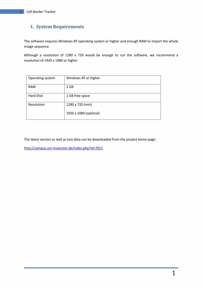
2. Installation of the CellBorderTracker package

Start the setup program.

Choose the installation path.

Accept the license agreement.

2 Cell Border Tracker

3

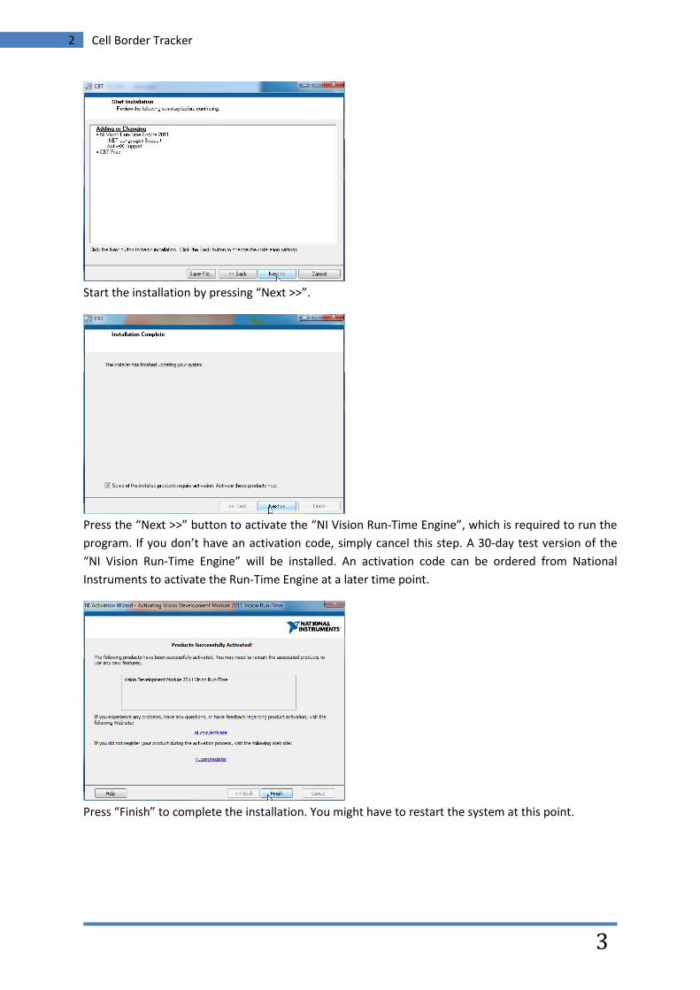
Start the installation by pressing “Next >>”.

Press the “Next >>” button to activate the “NI Vision Run-Time Engine”, which is required to run the program. If you don’t have an activation code, simply cancel this step. A 30-day test version of the “NI Vision Run-Time Engine” will be installed. An activation code can be ordered from National Instruments to activate the Run-Time Engine at a later time point.

Press “Finish” to complete the installation. You might have to restart the system at this point.

3 Cell Border Tracker

4

3. Image Segmentation with the CBE

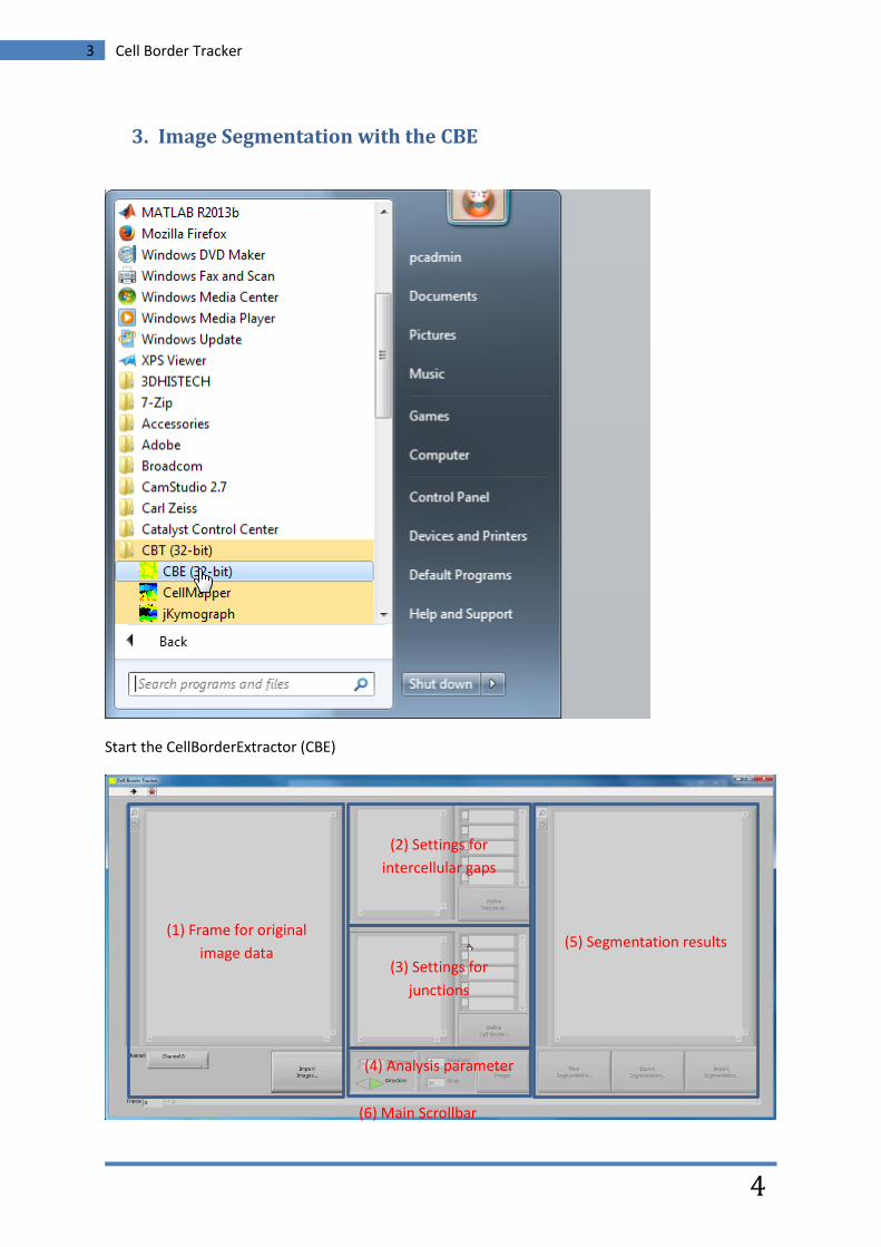
Start the CellBorderExtractor (CBE)

(1) Frame for original image data

(5) Segmentation results

(2) Settings for intercellular gaps

(3) Settings for junctions

(4) Analysis parameter

(6) Main Scrollbar

3 Cell Border Tracker

5

After starting the program the main window will appear. On the left side you will find a region where the original images will be displayed (1). In the middle area you can adjust parameters for the segmentation algorithm (2-4). The segmented images will appear on the right side (5). The main scroll bar allows you to scroll quickly through the image stacks (6). After importing the experimental data, one frame has to be segmented manually to “train” the program before the automated analysis can be started.

Before starting with the image analysis we strongly recommend that you watch the video tutorial (Supplementary Movie 1).

To familiarize you with the program we will use the example of a scratch experiment with endothelial cells expressing a VE-cadherin-EGFP construct. In this tutorial the steps used in analysing this example experiment will be explained in blue text. We strongly recommend that you follow these instructions closely when working with this software for the first time.

3.1 Importing the image data

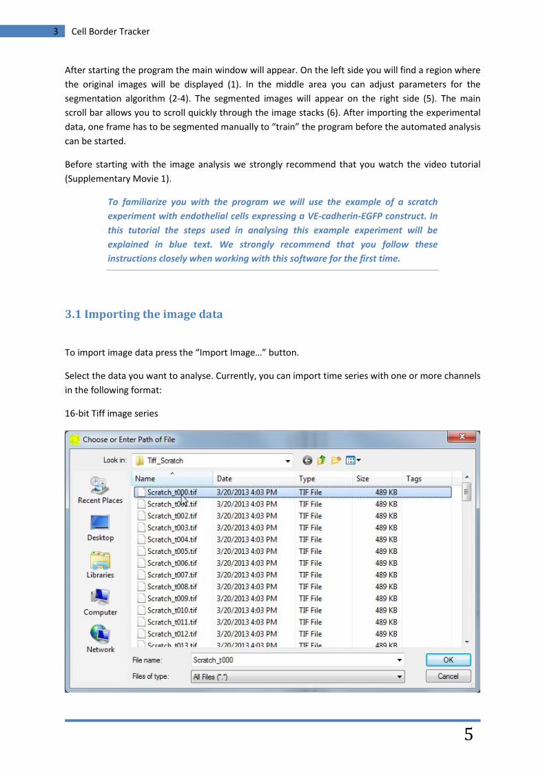
To import image data press the “Import Image…” button.

Select the data you want to analyse. Currently, you can import time series with one or more channels in the following format:

16-bit Tiff image series

3 Cell Border Tracker

6

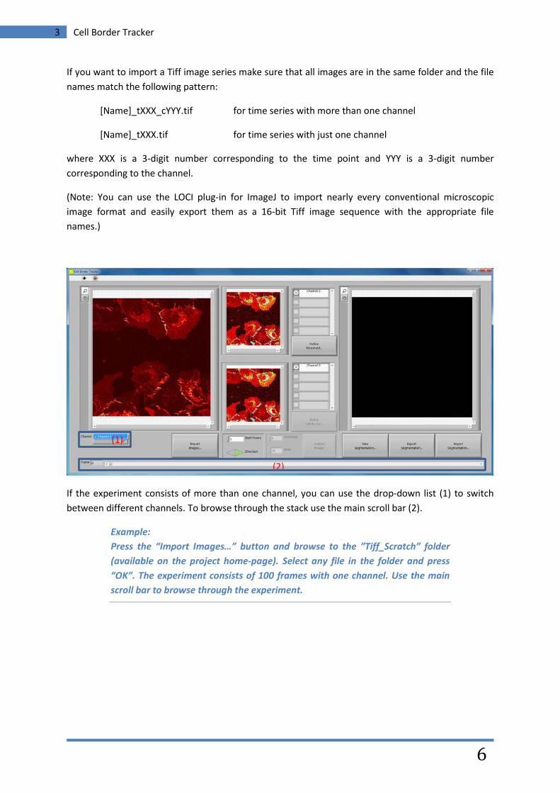
If you want to import a Tiff image series make sure that all images are in the same folder and the file names match the following pattern:

[Name]_tXXX_cYYY.tif for time series with more than one channel

[Name]_tXXX.tif for time series with just one channel

where XXX is a 3-digit number corresponding to the time point and YYY is a 3-digit number corresponding to the channel.

(Note: You can use the LOCI plug-in for ImageJ to import nearly every conventional microscopic image format and easily export them as a 16-bit Tiff image sequence with the appropriate file names.)

If the experiment consists of more than one channel, you can use the drop-down list (1) to switch between different channels. To browse through the stack use the main scroll bar (2).

Example: Press the “Import Images…” button and browse to the ”Tiff_Scratch” folder (available on the project home-page). Select any file in the folder and press “OK”. The experiment consists of 100 frames with one channel. Use the main scroll bar to browse through the experiment.

(1)

(2)

3 Cell Border Tracker

7

3.2 Setting parameters to identify intercellular gaps

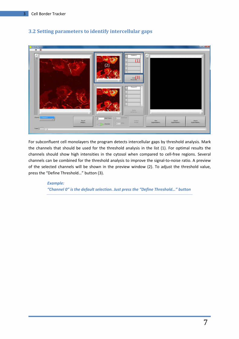
For subconfluent cell monolayers the program detects intercellular gaps by threshold analysis. Mark the channels that should be used for the threshold analysis in the list (1). For optimal results the channels should show high intensities in the cytosol when compared to cell-free regions. Several channels can be combined for the threshold analysis to improve the signal-to-noise ratio. A preview of the selected channels will be shown in the preview window (2). To adjust the threshold value, press the “Define Threshold…” button (3).

Example: “Channel 0” is the default selection. Just press the “Define Threshold…” button

(1) (2)

(3)

3 Cell Border Tracker

8

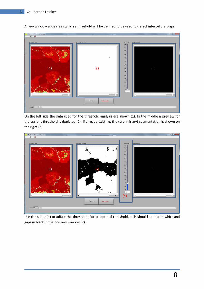
A new window appears in which a threshold will be defined to be used to detect intercellular gaps.

On the left side the data used for the threshold analysis are shown (1). In the middle a preview for the current threshold is depicted (2). If already existing, the (preliminary) segmentation is shown on the right (3).

Use the slider (4) to adjust the threshold. For an optimal threshold, cells should appear in white and gaps in black in the preview window (2).

(1) (2) (3)

(4)

(2) (1) (3)

3 Cell Border Tracker

9

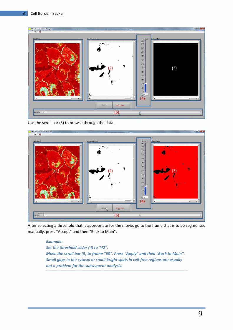
Use the scroll bar (5) to browse through the data.

After selecting a threshold that is appropriate for the movie, go to the frame that is to be segmented manually, press “Accept” and then “Back to Main”.

Example: Set the threshold slider (4) to “42”. Move the scroll bar (5) to frame “60”. Press “Apply” and then “Back to Main”. Small gaps in the cytosol or small bright spots in cell-free regions are usually not a problem for the subsequent analysis.

(5)

(4)

(2) (1) (3)

(4)

(2) (1) (3)

(5)

3 Cell Border Tracker

10

3.3 Setting the parameters for detection of junctions

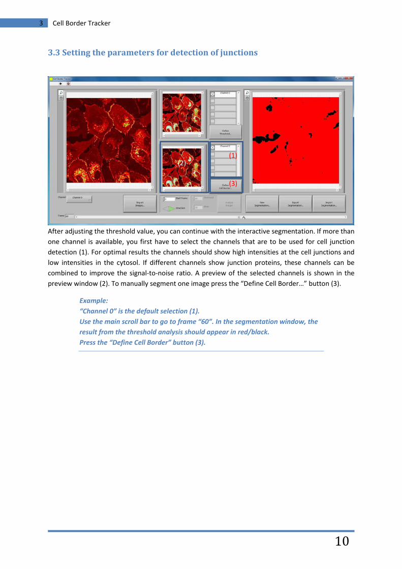
After adjusting the threshold value, you can continue with the interactive segmentation. If more than one channel is available, you first have to select the channels that are to be used for cell junction detection (1). For optimal results the channels should show high intensities at the cell junctions and low intensities in the cytosol. If different channels show junction proteins, these channels can be combined to improve the signal-to-noise ratio. A preview of the selected channels is shown in the preview window (2). To manually segment one image press the “Define Cell Border…” button (3).

Example: “Channel 0” is the default selection (1). Use the main scroll bar to go to frame “60”. In the segmentation window, the result from the threshold analysis should appear in red/black. Press the “Define Cell Border” button (3).

(1) (2)

(3)

3 Cell Border Tracker

11

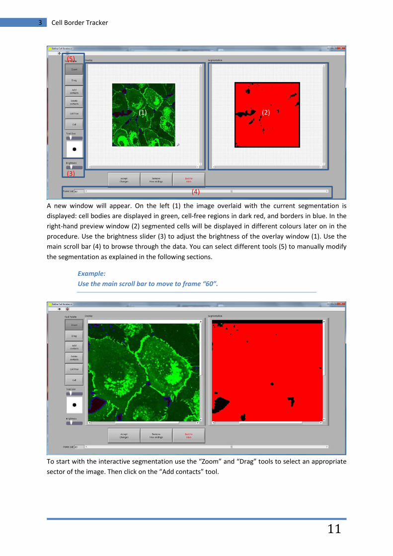
A new window will appear. On the left (1) the image overlaid with the current segmentation is displayed: cell bodies are displayed in green, cell-free regions in dark red, and borders in blue. In the right-hand preview window (2) segmented cells will be displayed in different colours later on in the procedure. Use the brightness slider (3) to adjust the brightness of the overlay window (1). Use the main scroll bar (4) to browse through the data. You can select different tools (5) to manually modify the segmentation as explained in the following sections.

Example: Use the main scroll bar to move to frame “60”.

To start with the interactive segmentation use the “Zoom” and “Drag” tools to select an appropriate sector of the image. Then click on the “Add contacts” tool.

(1) (2)

(3)

(4)

(5)

3 Cell Border Tracker

12

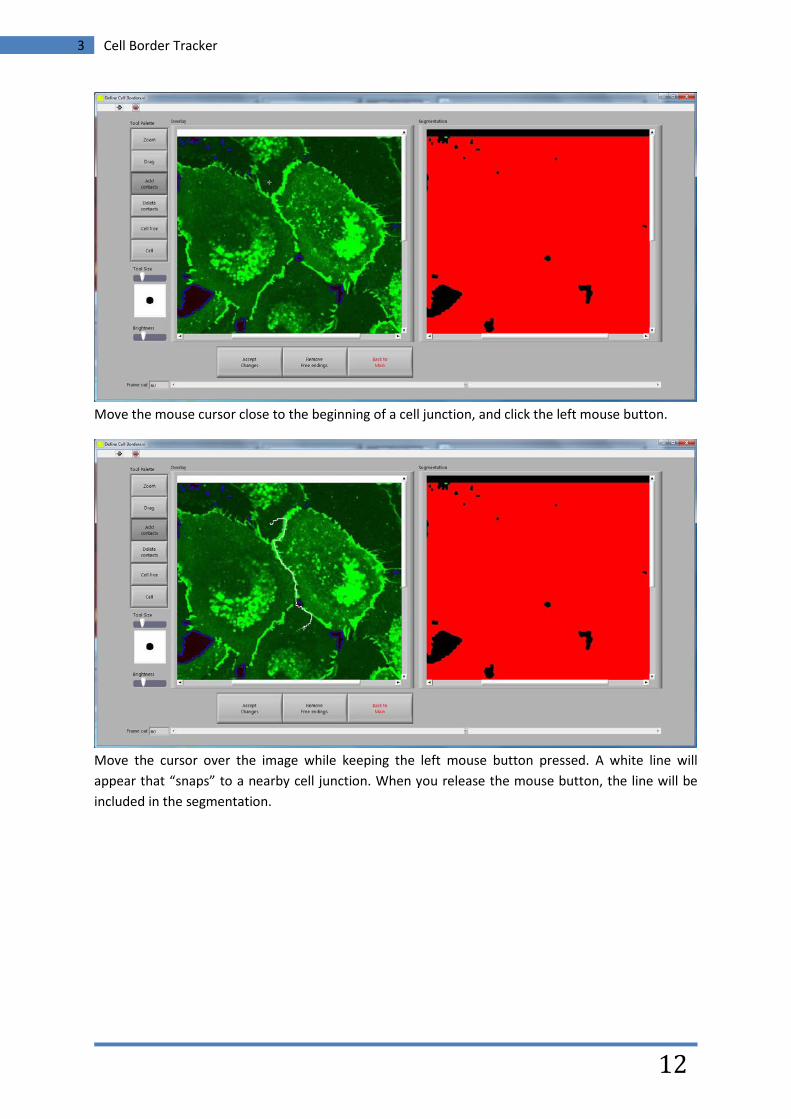
Move the mouse cursor close to the beginning of a cell junction, and click the left mouse button.

Move the cursor over the image while keeping the left mouse button pressed. A white line will appear that “snaps” to a nearby cell junction. When you release the mouse button, the line will be included in the segmentation.

3 Cell Border Tracker

13

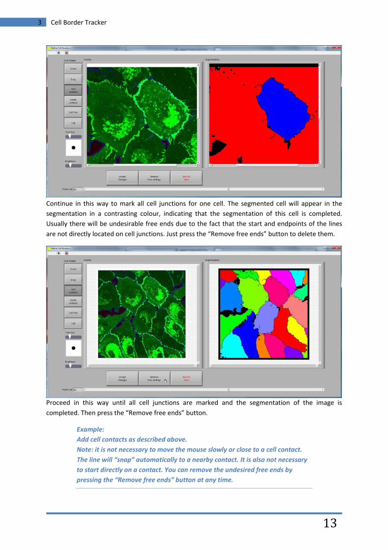
Continue in this way to mark all cell junctions for one cell. The segmented cell will appear in the segmentation in a contrasting colour, indicating that the segmentation of this cell is completed. Usually there will be undesirable free ends due to the fact that the start and endpoints of the lines are not directly located on cell junctions. Just press the “Remove free ends” button to delete them.

Proceed in this way until all cell junctions are marked and the segmentation of the image is completed. Then press the “Remove free ends” button.

Example: Add cell contacts as described above. Note: it is not necessary to move the mouse slowly or close to a cell contact. The line will “snap” automatically to a nearby contact. It is also not necessary to start directly on a contact. You can remove the undesired free ends by pressing the “Remove free ends” button at any time.

3 Cell Border Tracker

14

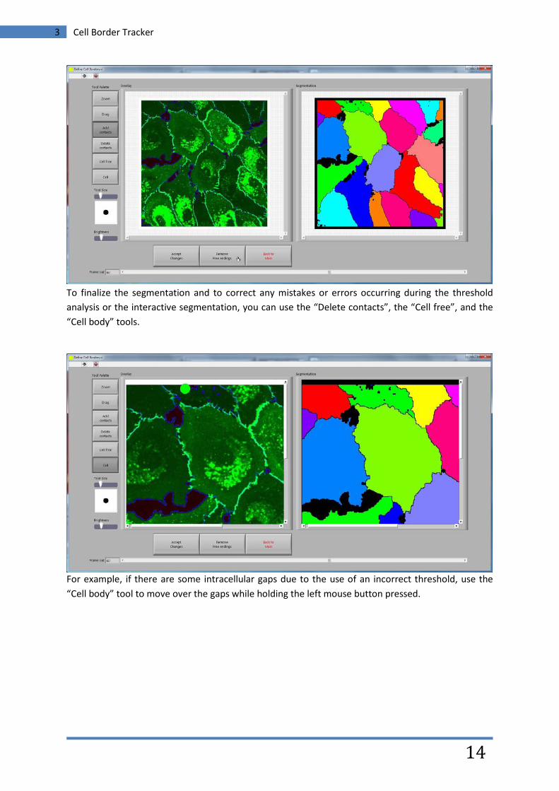
To finalize the segmentation and to correct any mistakes or errors occurring during the threshold analysis or the interactive segmentation, you can use the “Delete contacts”, the “Cell free”, and the “Cell body” tools.

For example, if there are some intracellular gaps due to the use of an incorrect threshold, use the “Cell body” tool to move over the gaps while holding the left mouse button pressed.

3 Cell Border Tracker

15

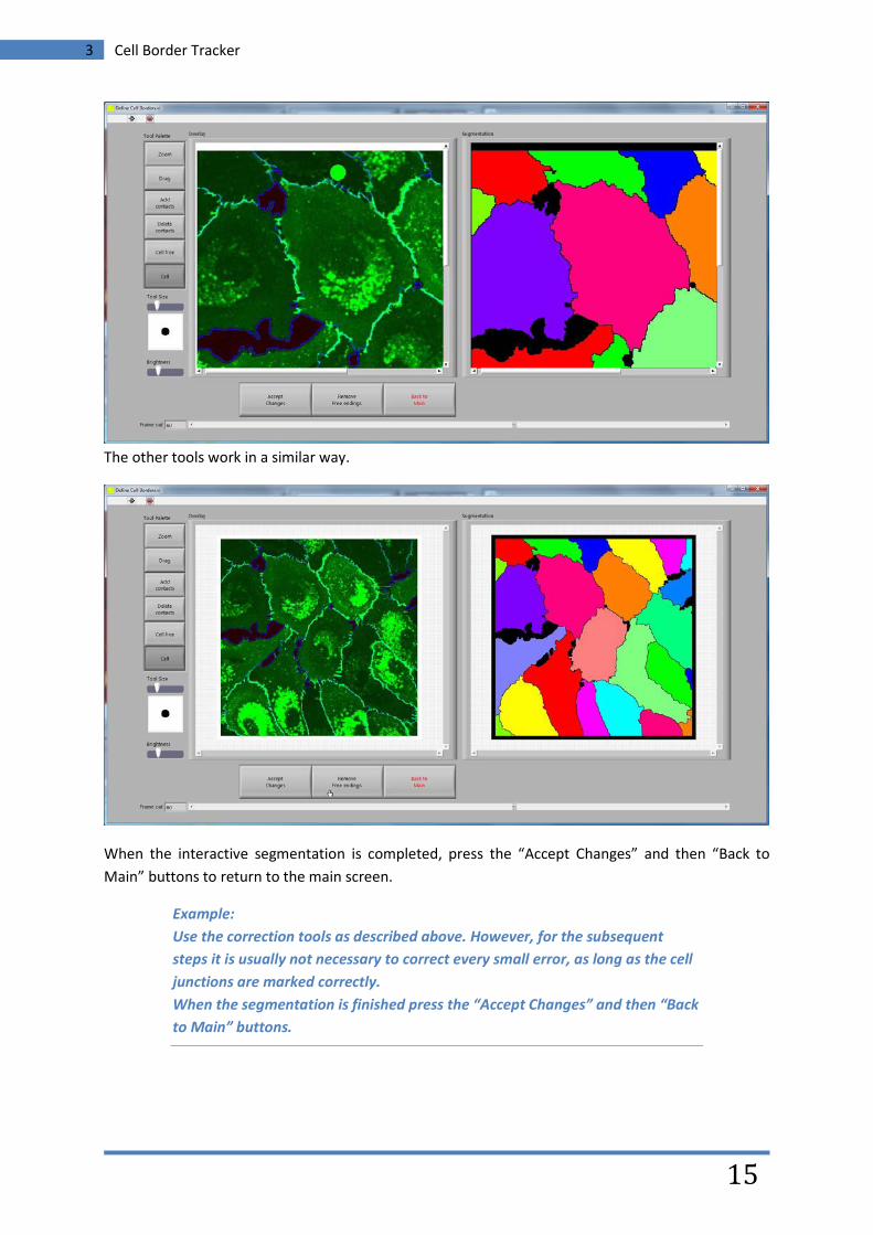
The other tools work in a similar way.

When the interactive segmentation is completed, press the “Accept Changes” and then “Back to Main” buttons to return to the main screen.

Example: Use the correction tools as described above. However, for the subsequent steps it is usually not necessary to correct every small error, as long as the cell junctions are marked correctly. When the segmentation is finished press the “Accept Changes” and then “Back to Main” buttons.

3 Cell Border Tracker

16

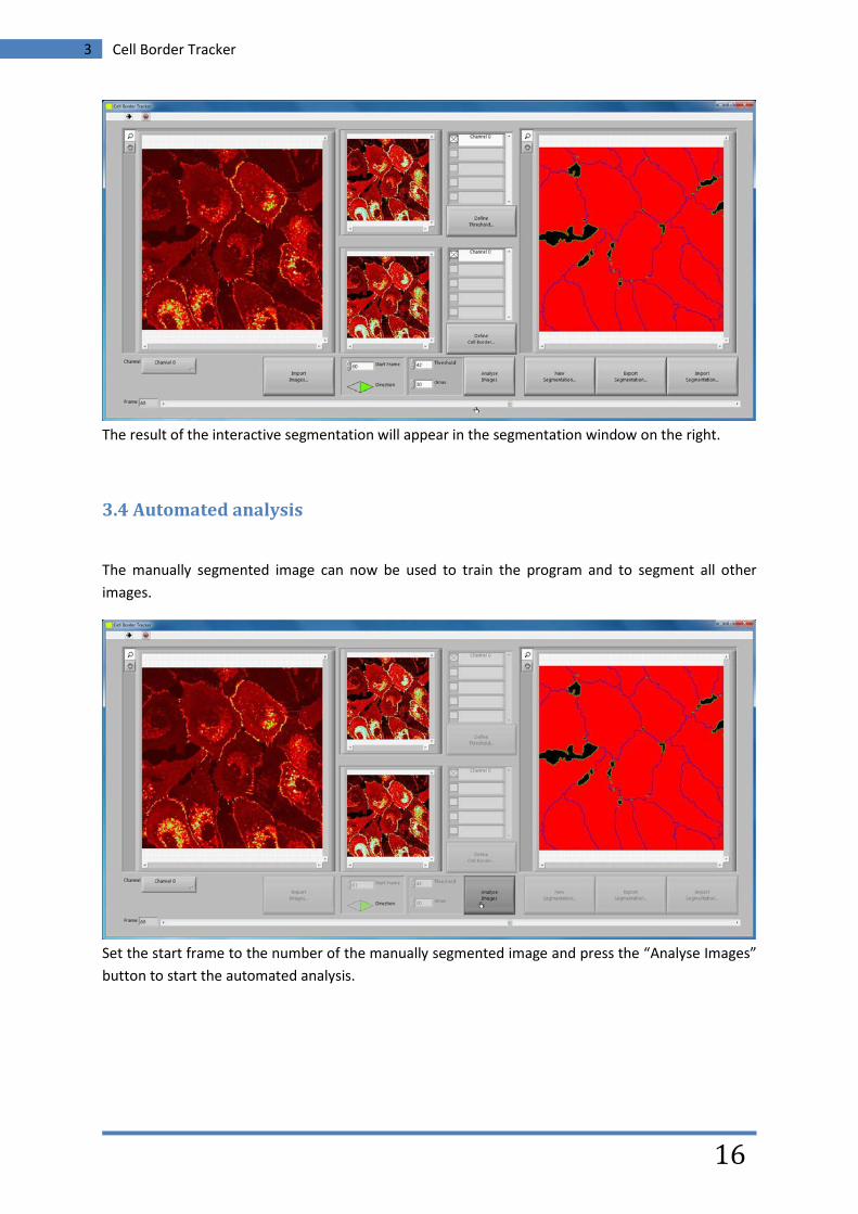
The result of the interactive segmentation will appear in the segmentation window on the right.

3.4 Automated analysis

The manually segmented image can now be used to train the program and to segment all other images.

Set the start frame to the number of the manually segmented image and press the “Analyse Images” button to start the automated analysis.

3 Cell Border Tracker

17

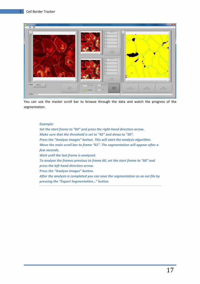
You can use the master scroll bar to browse through the data and watch the progress of the segmentation.

Example: Set the start frame to “60” and press the right-hand direction arrow. Make sure that the threshold is set to “42” and dmax to “20”. Press the “Analyse Images” button. This will start the analysis algorithm. Move the main scroll bar to frame “61”. The segmentation will appear after a few seconds. Wait until the last frame is analysed. To analyse the frames previous to frame 60, set the start frame to “60” and press the left-hand direction arrow. Press the “Analyse Images” button. After the analysis is completed you can save the segmentation as an avi file by pressing the “Export Segmentation…” button

3 Cell Border Tracker

18

3.5 Exporting the segmentations

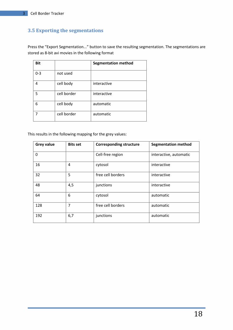
Press the “Export Segmentation...” button to save the resulting segmentation. The segmentations are stored as 8-bit avi movies in the following format

Bit Segmentation method

0-3 not used

4 cell body interactive

5 cell border interactive

6 cell body automatic

7 cell border automatic

This results in the following mapping for the grey values:

Grey value Bits set Corresponding structure Segmentation method

0 Cell-free region interactive, automatic

16 4 cytosol interactive

32 5 free cell borders interactive

48 4,5 junctions interactive

64 6 cytosol automatic

128 7 free cell borders automatic

192 6,7 junctions automatic

3 Cell Border Tracker

19

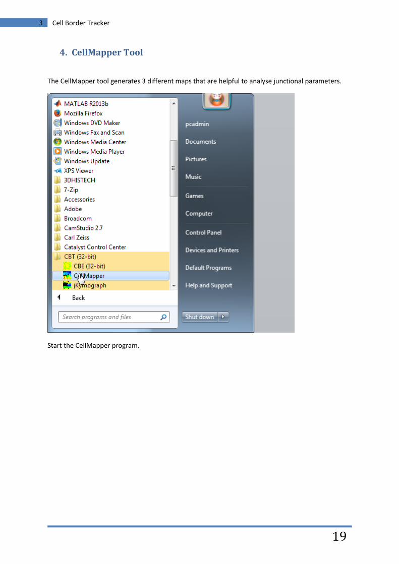
4. CellMapper Tool

The CellMapper tool generates 3 different maps that are helpful to analyse junctional parameters.

Start the CellMapper program.

3 Cell Border Tracker

20

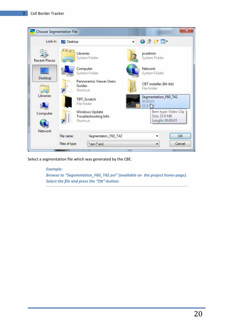
Select a segmentation file which was generated by the CBE.

Example: Browse to “Segemntation_F60_T42.avi” (available on the project home-page). Select the file and press the “OK”-button.

3 Cell Border Tracker

21

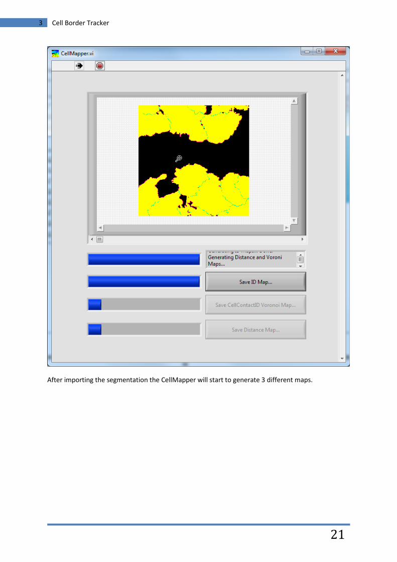
After importing the segmentation the CellMapper will start to generate 3 different maps.

3 Cell Border Tracker

22

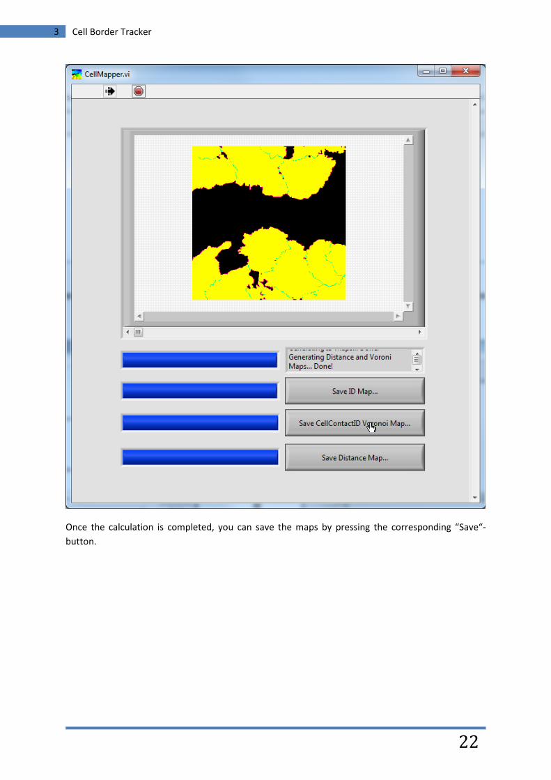
Once the calculation is completed, you can save the maps by pressing the corresponding “Save“-button.

3 Cell Border Tracker

23

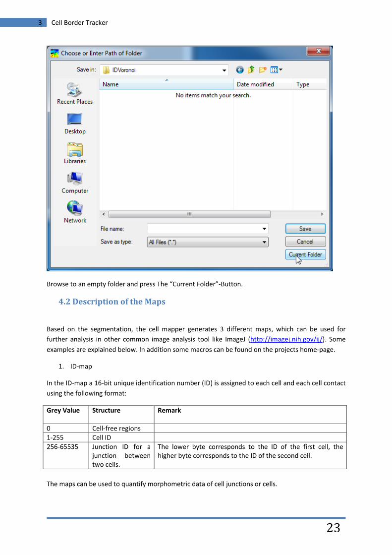
Browse to an empty folder and press The “Current Folder”-Button.

4.2 Description of the Maps

Based on the segmentation, the cell mapper generates 3 different maps, which can be used for further analysis in other common image analysis tool like ImageJ (http://imagej.nih.gov/ij/). Some examples are explained below. In addition some macros can be found on the projects home-page.

1. ID-map

In the ID-map a 16-bit unique identification number (ID) is assigned to each cell and each cell contact using the following format:

The maps can be used to quantify morphometric data of cell junctions or cells.

Grey Value

Structure Remark

0 Cell-free regions 1-255 Cell ID 256-65535 Junction ID for a

junction between two cells.

The lower byte corresponds to the ID of the first cell, the higher byte corresponds to the ID of the second cell.

3 Cell Border Tracker

24

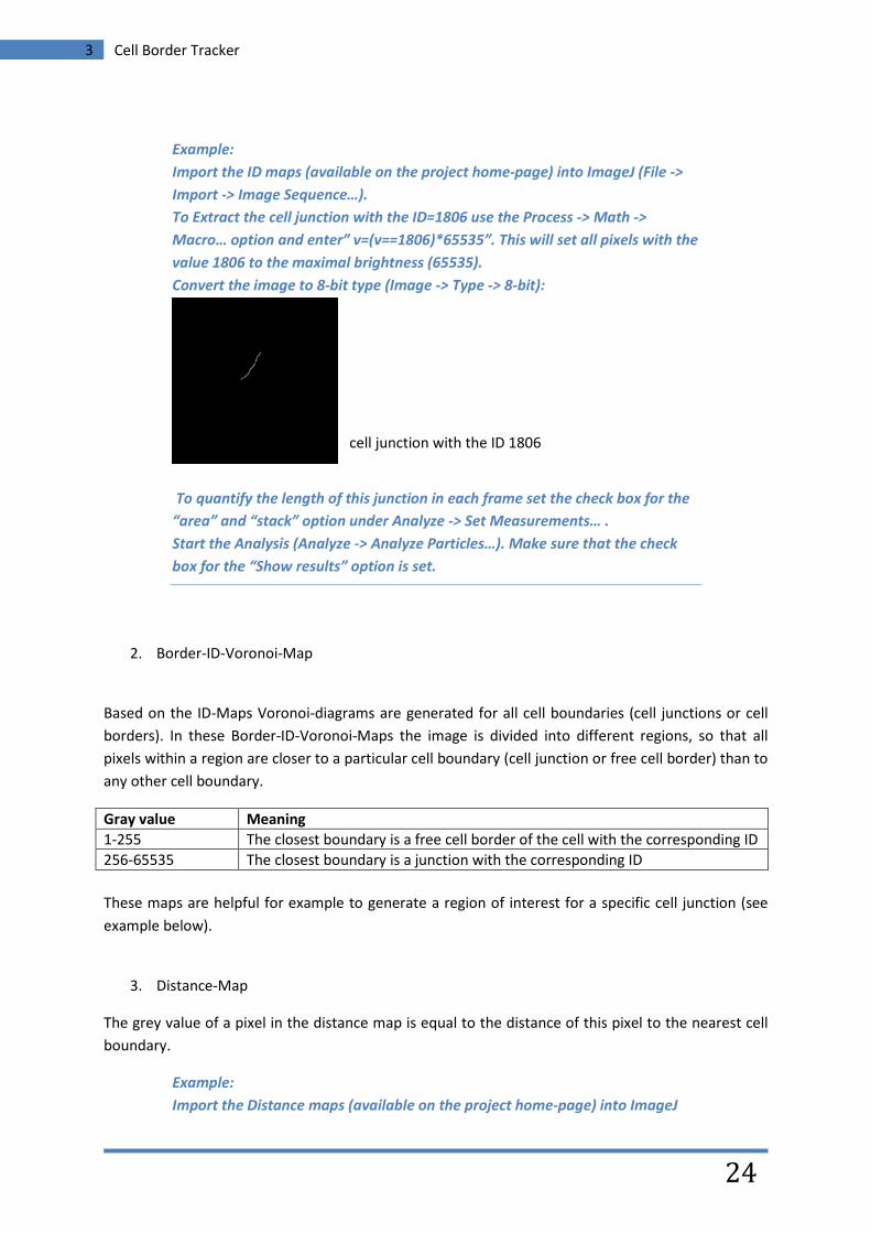
Example: Import the ID maps (available on the project home-page) into ImageJ (File -> Import -> Image Sequence…). To Extract the cell junction with the ID=1806 use the Process -> Math -> Macro… option and enter” v=(v==1806)*65535”. This will set all pixels with the value 1806 to the maximal brightness (65535). Convert the image to 8-bit type (Image -> Type -> 8-bit):

To quantify the length of this junction in each frame set the check box for the “area” and “stack” option under Analyze -> Set Measurements… . Start the Analysis (Analyze -> Analyze Particles…). Make sure that the check box for the “Show results” option is set.

2. Border-ID-Voronoi-Map

Based on the ID-Maps Voronoi-diagrams are generated for all cell boundaries (cell junctions or cell borders). In these Border-ID-Voronoi-Maps the image is divided into different regions, so that all pixels within a region are closer to a particular cell boundary (cell junction or free cell border) than to any other cell boundary.

Gray value Meaning 1-255 The closest boundary is a free cell border of the cell with the corresponding ID 256-65535 The closest boundary is a junction with the corresponding ID These maps are helpful for example to generate a region of interest for a specific cell junction (see example below).

3. Distance-Map

The grey value of a pixel in the distance map is equal to the distance of this pixel to the nearest cell boundary.

Example: Import the Distance maps (available on the project home-page) into ImageJ

cell junction with the ID 1806

3 Cell Border Tracker

25

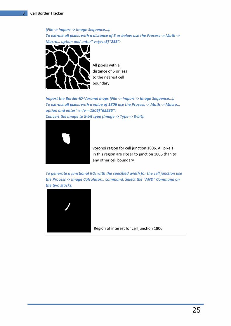
(File -> Import -> Image Sequence…). To extract all pixels with a distance of 5 or below use the Process -> Math -> Macro… option and enter” v=(v<=5)*255”:

Import the Border-ID-Voronoi maps (File -> Import -> Image Sequence…). To extract all pixels with a value of 1806 use the Process -> Math -> Macro… option and enter” v=(v==1806)*65535”. Convert the image to 8-bit type (Image -> Type -> 8-bit):

To generate a junctional ROI with the specified width for the cell junction use the Process -> Image Calculator… command. Select the “AND” Command on the two stacks:

voronoi region for cell junction 1806. All pixels in this region are closer to junction 1806 than to any other cell boundary

Region of interest for cell junction 1806

All pixels with a distance of 5 or less to the nearest cell boundary

3 Cell Border Tracker

26

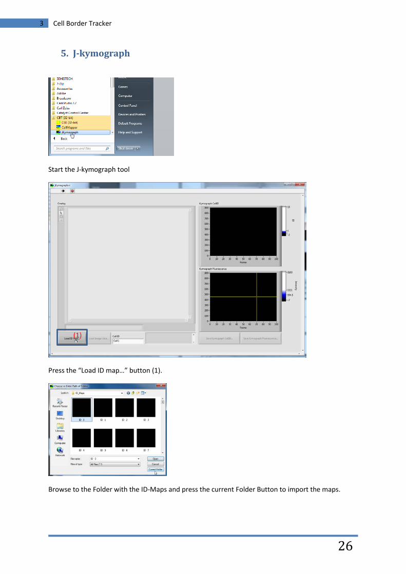
5. J-kymograph

Start the J-kymograph tool

Press the “Load ID map…” button (1).

Browse to the Folder with the ID-Maps and press the current Folder Button to import the maps.

(1)

3 Cell Border Tracker

27

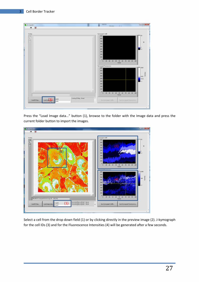
Press the “Load Image data…” button (1), browse to the folder with the Image data and press the current folder button to import the images.

Select a cell from the drop down field (1) or by clicking directly in the preview image (2). J-kymograph for the cell IDs (3) and for the Fluorescence Intensities (4) will be generated after a few seconds.

(1)

(2)

(1)

(3)

(4)

3 Cell Border Tracker

28

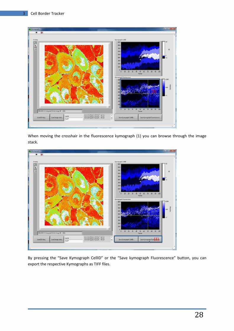
When moving the crosshair in the fluorescence kymograph (1) you can browse through the image stack.

By pressing the “Save Kymograph CellID” or the “Save kymograph Fluorescence” button, you can export the respective Kymographs as TIFF files.

(1)

(1)