A three-dimensional finite element model and image reconstruction algorithm for time-domain

fluorescence imaging in highly scattering media

This article has been downloaded from IOPscience. Please scroll down to see the full text article.

2011 Phys. Med. Biol. 56 7419

(http://iopscience.iop.org/0031-9155/56/23/006)

Download details:

IP Address: 147.188.200.249

The article was downloaded on 25/06/2012 at 09:23

Please note that terms and conditions apply.

View the table of contents for this issue, or go to the journal homepage for more

Home Search Collections Journals About Contact us My IOPscience

IOP PUBLISHING PHYSICS IN MEDICINE AND BIOLOGY

Phys. Med. Biol. 56 (2011) 7419–7434 doi:10.1088/0031-9155/56/23/006

A three-dimensional finite element model and imagereconstruction algorithm for time-domainfluorescence imaging in highly scattering media

Q Zhu1, H Dehghani1, K M Tichauer2, R W Holt3, K Vishwanath4,F Leblond2 and B W Pogue2

1 School of Computer Science, University of Birmingham, Birmingham, B15 2TT, UK2 Thayer School of Engineering, Dartmouth College, NH 03755, USA3 Department of Physics and Astronomy, Dartmouth College, NH 03755, USA4 Department of Biomedical Engineering, Duke University, Durham, NC 27708, USA

E-mail: h.dehghani@cs.bham.ac.uk

Received 27 June 2011, in final form 14 October 2011Published 4 November 2011Online at stacks.iop.org/PMB/56/7419

AbstractIn this work, development and evaluation of a three-dimensional (3D)finite element model (FEM) based on the diffusion approximation of time-domain (TD) near-infrared fluorescence light transport in biological tissueis presented. This model allows both excitation and fluorescence temporalpoint-spread function (TPSF) data to be generated for heterogeneous scatteringand absorbing media of arbitrary geometry. The TD FEM is evaluated viacomparisons with analytical and Monte Carlo (MC) calculations and is shownto provide a quantitative accuracy which has less than 0.72% error in intensityand less than 37 ps error for mean time. The use of the Born–Ratio normalizeddata is demonstrated to reduce data mismatch between MC and FEM to less than0.22% for intensity and less than 22 ps in mean time. An image reconstructionframework, based on a 3D FEM formulation, is outlined and simulation resultsbased on a heterogeneous mouse model with a source of fluorescence inthe pancreas is presented. It is shown that using early photons (i.e. thephotons detected within the first 200 ps of the TPSF) improves the spatialresolution compared to using continuous-wave signals. It is also demonstrated,as expected, that the utilization of two time gates (early and latest photons) canimprove the accuracy both in terms of spatial resolution and recovered contrast.

(Some figures in this article are in colour only in the electronic version)

1. Introduction

Time-domain (TD) near-infrared (NIR) fluorescence imaging is a molecular imaging techniquewhereby a region of interest is irradiated by a red or NIR excitation light source and the

0031-9155/11/237419+16$33.00 © 2011 Institute of Physics and Engineering in Medicine Printed in the UK 7419

7420 Q Zhu et al

emitted fluorescence light, together with the transmitted and/or reflected light at excitation,is used to determine the spatial distributions of fluorescent tracers and/or other fluorescentstructures in biological tissue (Arridge et al 1993, Gao et al 2006, 2008, Kumar et al 2006,Lam et al 2005, Leblond et al 2009, Niedre and Ntziachristos 2010, Patterson and Pogue1994, Soloviev et al 2007, Vishwanath and Mycek 2005). Although the comparison betweenthe different data collection strategies is largely under debate, continuous-wave (CW) andfrequency-domain (FD) systems have to date been relatively inexpensive, less complex todevelop and have provided relatively shorter time scans, whereas TD systems are slow (dueto photon counting nature) but highly sensitive. It is also well accepted that since TD andFD systems provide time-resolved information, it is possible to independently measure thedistribution of both scattering and absorption coefficients, as well as fluorescence lifetime(O’Leary et al 1996). Additionally, a theoretical analysis of the moments of the forwardproblem in fluorescence diffuse optical tomography through use of different data types for TRfluorescence reconstruction has demonstrated the increasing sensitivity of moments to noise(Ducros et al 2009). However, since TD measurement data implicitly contain a weightedsum of modulation frequencies from the FD data types, it can in principle provide muchmore information regarding the underlying optical properties of the tissue being interrogated(Marjono et al 2008).

The benefits of using early arriving photons have been long known (Wu et al 1997), and anumber of researchers have previously studied and developed TD-based image reconstructionstrategies that utilize time-gated data to extract optical properties from the domain beingimaged (Kumar et al 2005, Gao et al 2002). The use of early photons can potentially leadto a better imaging resolution, through the reduction in thickness of the photon measurementdensity function for early sampling times (Schweiger and Arridge 1995). Additionally, therehas been some work describing the use of a gradient-based iterative reconstruction schemewith multiple time gates over the full TD curve (Hielscher et al 1999). More recently, Niedreet al (Niedre et al 2008, Li and Niedre 2011) have demonstrated that improvements inresolution can be achieved by the use of early photons for fluorescence tomographic imagingof lung tumors in mice in vivo. Further studies have shown that when transmitted through thetorso of a mouse, early photons were significantly less diffuse than quasi-CW photons, whichallowed an improved visualization of fluorescent targets for individual optical projections andreconstructed tomographic images (Niedre and Ntziachristos 2010). Leblond et al (2009) havealso demonstrated that early photon data allow the improvement of spatial resolution, since itallows the retention of imaging singular modes corresponding to higher spatial frequencies inthe image reconstruction problem.

For clinical applications, TD imaging can potentially be used to develop a non-invasivein vivo molecular imaging technique that not only allows real-time viewing of cellular activitybut is also able to extract time-related patho-physiological information from biological tissue(Luker and Luker 2008, Zhang et al 2007, Massoud et al 2004). The technique could beapplied for diseases such as cancer detection and diagnosis at a very early stage in comparisonwith other imaging or detection modalities that require months or years for tumors to grow tobe detectable (Palmedo et al 2002, Houston et al 1988, Warner et al 2001). This provides theadvantages of faster treatment of the diseases and better therapeutic monitoring and outcomes.In addition, the model in practice could also potentially be used to accelerate drug discoveryand development due to its ability of nearly real-time viewing of cellular activity in vivo (Lukerand Luker 2008, Rudin and Weissleder 2003, Gross and Piwnica-Worms 2006).

To date, much work relating to TD fluorescent modeling has been done; however, theyare mostly centered on 2D light transport models (Gao et al 2006, 2008), and most havebeen developed for FD systems (Jiang 1998, Lee and Sevick-Muraca 2002). The algorithms

A 3D FEM and image reconstruction algorithm for TD fluorescence imaging in highly scattering media 7421

and techniques presented in this paper are developed for three-dimensional (3D) fluorescentmodels using finite element models (FEM) for TD propagation of NIR light in turbid media.In addition, analytical solutions (Lam et al 2005, Patterson and Pogue 1994, Hattery et al2001) and Monte Carlo (MC) (Vishwanath and Mycek 2005) models have also been usedfor simulations of 3D fluorescent light propagation in TD that can provide model verification.However, analytical solutions provide fast and computationally efficient solutions but typicallysuffer from the drawback that they can only be applied for simple homogeneous geometries,although some developments of analytical solutions based on Kirchoff’s approximation forfluorescence models have been reported (Ripoll et al 2002). MC models, on the other hand, canbe applied for complex geometries; however, these approaches are more time consuming andcomputationally expensive to achieve stable responses (Preisa et al 2009, Fang and Boas 2009),but with the advent of graphics processing unit (GPU) and parallel processing implementationthe processing time has been dramatically improved (Fang and Boas 2009, Jin et al 2011).The FEM introduced in this paper combines the strengths of both these approaches, providinga fast technique that can be applied for complex heterogeneous geometries.

In this paper, we outline in detail the implementation of 3D TD FEM-based fluorescencemodel and its validation via MC and analytical simulations. Specifically, we demonstrate theaccuracy of the application of the fluorescence TD FEM using the diffusion approximation(DA), as compared to both an analytical model (also based on the DA) and an MC modelusing a 3D slab reflectance model. The measured temporal point-spread functions (TPSFs)for both the excitation and emission data are compared against the two models (i.e. analyticaland MC) to demonstrate the limits of the DA on TD data, as well as to outline the benefits ofusing the so-called Born–Ratio (emission normalized with respect to excitation) data. Whencompared to MC, the FEM Born–Ratio data are shown to provide a greater degree of accuracyin terms of data match than the FEM fluorescence data alone. Data are also presented showingthat the early time-bin intensity measurements as acquired from a TD model are a functionof the source/detector separation, though this does not necessarily imply that the accuracy ofshorter time-bins increases with source/detector separation. Finally, the FEM-based imagereconstruction algorithm that can be used for time-gated intensity data is also presented indetail together with the incorporation of multiple time-bins for 3D tomographic imagingof a complex mouse model. The models and algorithms presented were developed using theNIRFAST software (Dehghani et al 2008), which is an open source software package designedfor light transport modeling and image reconstruction.

2. Methods and results

2.1. FEM solutions to the time-dependent diffusion equation

Although generally well known and understood, in order to outline the implementation of boththe forward and inverse model for TD fluorescence within the FEM framework, we will firstdefine the DA. In the following, the subscripts x and m denote the excitation and fluorescenceemission wavelengths, respectively, of a light field propagating within a heterogeneous turbidmedium, �. The medium is excited using an ultra-short point source, which is modeled using adelta-function source, δ(r−rs, t), along the space and time dimensions. The propagation of bothexcitation and emission light in the medium can be modeled by two coupled time-dependentdiffusion equations:[

∇ · κx(r)∇ − (μax(r) + μaf(r))c − ∂

∂t

]φx(r, rs, t) = −δ(r − rs, t), (1)

7422 Q Zhu et al[∇ · κm(r)∇ − μam(r)c − ∂

∂t

]φm(rd, r, t) = −η(r)

τ (r)c[φx(r, rs, t) ⊗ exp(τ (r), t)], (2)

where φv(r, rg, t) (v∈[x, m], g∈[s, d]) are the time-dependent photon density functions attime t and position r. The field φx(r, rs, t) is the impulse/tissue response to a delta-functionsource of wavelength λx located at position rs. On the other hand, φm(rd, r, t) models the lightsignal detected at position rd resulting from fluorescence emitted by a fluorophore distributionwith absorption coefficient μaf(r) located at position r. The photon density functions dependnonlinearly on the effective tissue optical properties, namely the absorption coefficient, μav(r),and the diffusion coefficient, κv(r, t) = 1/[3(μav(r) + μ′

sv(r)], where μ′sv(r) is the reduced

scattering coefficient. The photon density at the excitation wavelength, φx(r, rs, t), is also anonlinear function of the fluorophore absorption coefficient, μaf(r); however, it is customary,when using diffused fluorescence to image tissue, to assume that the fluorophore absorptioncoefficient is much smaller than that associated with other chromophores such as hemoglobinand water. As a consequence, equation (1) is often solved assuming that the fluence functionsare independent of μaf(r) (Gao et al 1998, Lam et al 2005, Niedre et al 2008), whereas, inthis work the potential nonlinear dependence of φx(r, rs, t) on μaf(r) is accounted for. It isassumed that there is negligible overlap between the excitation and emission spectra of thefluorophore at λm and therefore the emission photon density is assumed to be independent ofμaf(r). The other physical parameters characterizing the fluorophores are the lifetime, τ (r),and the quantum efficiency, η(r). In equation (2), exp(τ , t) = e−t/τ (r)U(t), where U(t) is aunit-step function and the operator ⊗ is the temporal convolution operator. Solutions to theequations above are obtained using type III boundary conditions, which have been shown toaccurately account for the index of refraction mismatch at the air/tissue boundary (Schweigeret al 1995).

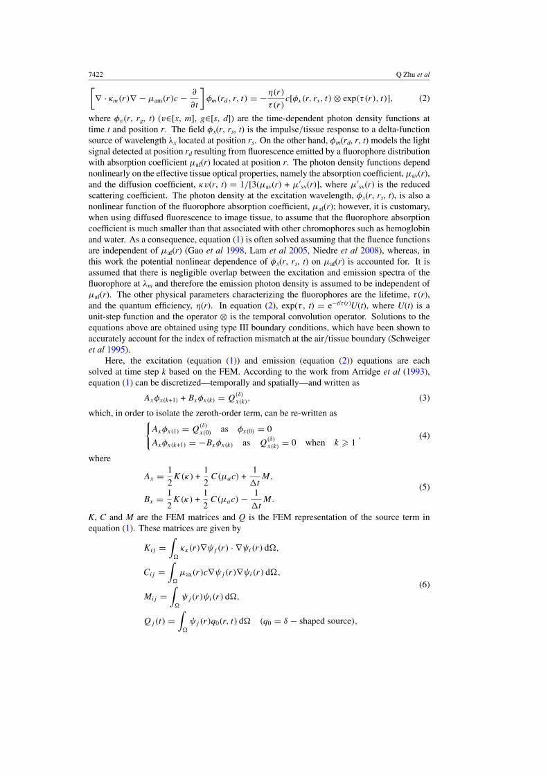
Here, the excitation (equation (1)) and emission (equation (2)) equations are eachsolved at time step k based on the FEM. According to the work from Arridge et al (1993),equation (1) can be discretized—temporally and spatially—and written as

Axφx(k+1) + Bxφx(k) = Q(δ)

x(k), (3)

which, in order to isolate the zeroth-order term, can be re-written as{Axφx(1) = Q

(δ)

x(0) as φx(0) = 0

Axφx(k+1) = −Bxφx(k) as Q(δ)

x(k) = 0 when k � 1, (4)

where

Ax = 1

2K(κ) +

1

2C(μac) +

1

tM,

Bx = 1

2K(κ) +

1

2C(μac) − 1

tM.

(5)

K, C and M are the FEM matrices and Q is the FEM representation of the source term inequation (1). These matrices are given by

Kij =∫

�

κx(r)∇ψj(r) · ∇ψi(r) d�,

Cij =∫

�

μax(r)c∇ψj(r)∇ψi(r) d�,

Mij =∫

�

ψj (r)ψi(r) d�,

Qj(t) =∫

�

ψj (r)q0(r, t) d� (q0 = δ − shaped source),

(6)

A 3D FEM and image reconstruction algorithm for TD fluorescence imaging in highly scattering media 7423

where ψ is the basis function and i, j = 1, 2, 3, · · ·, N, and N is the number of nodeswithin the FEM volume mesh. FEM solutions to equation (1) are obtained by solvingequation (4) through matrix inversion, which is achieved using a bi-conjugate gradient solverwith a pre-conditioner based on one Choleski factorization of the matrix Ax.

Solutions for the emission case are obtained in a manner similar to the excitation casewith the exception of the source term, which is now a function of the FEM fields φx(k). First,equation (2) is written in the form

Amφm(k+1) + Bmφm(k) = Qm(k+1), (7)

where

Qm(r) = −η(r)

τ (r)c[φx(r, rs, t) ⊗ e−t/τ ]

= [Qm(1),Qm(2),Qm(3), . . . , Qm(k)]. (8)

Equation (7) can then be re-written as{Amφm(1) = Qm(1) as φm(0) = 0, k = 0Amφm(k+1) = Qm(k+1) − Bmφm(k) k � 1

(9)

where the structure of the matrices, Am and Bm, is the same as those defined in equation (5),with the exception that the optical properties that are used to evaluate the matrices are thoseassociated with the emission wavelength, λm.

The main difference between equations (4) and (9) is the source term on the right-handside. For the excitation case, the laser source is approximated by a delta function. However,the source term for the emission case depends on the physical properties of the fluorescentmolecules as well as on the spatial and temporal distributions of the excitation field, φx. Inorder to obtain FEM solutions for the excitation field, the first time-step intensity (φx(1)) isinitially obtained by solving equation (4) with the delta-function source. Then, as shown byinspection of equation (4), the calculated solution at time step, k = 1, is used as the sourceterm for calculating the intensity in the next time step (k = 2). This process is repeatediteratively in order to compute the modeled light intensity for every time step until the end ofthe modeled photo-detection time window. For the emission case, the first time-step intensity,φm(1), is obtained by solving equation (9). Prior to solving this equation, however, a timeconvolution operation between the mathematical objects φx(1) and exp(τ , t) is numericallyperformed. Then, the resulting time-vector is multiplied by the ratio of the quantum efficiencyand the lifetime, η(r)/τ (r). The light intensities for all time steps are then derived using asimilar approach as defined for the excitation case.

Validation of the TD algorithm presented was achieved by direct comparison of the time-dependent FEM solutions against both analytical solutions and MC simulations. The particularanalytical and MC models used here have been shown in the past to accurately model lighttransport in tissue for epi-illumination detection geometries (see, e.g., Leblond et al (2010a)for a description of the various detection geometries used in diffuse fluorescence imaging).As such, those methods can be considered gold standards for light transport simulationsin biological tissue. The analytical model is a closed-form solution to the time-dependentdiffusion equation assuming extrapolated boundary conditions consistent with a single-layersemi-infinite turbid medium and is based on the work of Patterson and Pogue (1994). The MCmodel used here was developed by Vishwanath and Mycek (2005), and is able to simulate TDsignals (i.e. TPSFs) at both excitation and fluorescence emission wavelengths in a multi-layeredsemi-infinite turbid medium. However, contrary to numerical FEM solutions and analyticalmodeling, MC simulations are obtained using a statistical approach. As such, the requirementfor acceptable levels of signal-to-noise ratio (SNR) imposes that each simulation keeps track

7424 Q Zhu et al

Table 1. Optical properties and fluorophore physical parameters associated with the tissue-mimicking numerical phantom used for epi-illumination photo-detection simulations. The reducedscattering coefficient used for the FEM and analytical simulations is given as μs′ = (1−g)μs.

Epi-illumination numerical phantom optical properties

Physical parameter Symbol Measured value

Absorption coefficient (excitation) μax 0.035 mm−1

Absorption coefficient (emission) μam 0.035 mm−1

Scattering coefficient (excitation) μsx 10.0 mm−1

Scattering coefficient (emission) μsm 10.0 mm−1

Scattering anisotropy factor (excitation) gx 0.9Scattering anisotropy factor (emission) gm 0.9Fluorophore absorption coefficient (excitation) μaf 0.0019 mm−1

Fluorophore quantum yield η 0.1Fluorophore lifetime τ 1 nsIndex of refraction n 1.52

of large numbers of photons typically of the order of 1 × 106 and more. This explains why MCsimulations can result in prohibitively large computational times and memory requirementswhen compared to numerical FEM and analytical approaches; although with the current adventof low cost GPU computation these computational times have improved (Fang and Boas 2009).

Bench-marking of the FEM against the analytical and MC solutions was achievedassuming an epi-illumination photo-detection geometry. Tissue excitation was modeled asa narrow beam source and light detection was modeled at a single point located a distanced away from the light source. The geometry of a semi-infinite homogeneous turbid mediumwas used for the analytical and MC solutions, whereas, the FEM numerical solutions wereobtained using the mesh of a rectangular cuboid. The physical dimensions of the cuboidwere x = 135 mm, y = 40 mm and z = 60 mm with a mesh resolution of 0.85 mm.More precisely, the ranges of the cuboid spatial coordinates were x = [50 mm : −85 mm],y = [0 mm : −40 mm] and z = [−30 mm : 30 mm], with a nodal spacing of 0.85 mm.

For all simulations (analytical, statistical and numerical), the excitation laser source wasmodeled on the surface at (x,y,z) = (0,0,0) mm, i.e., on the same surface where measurementsare made for source–detector distances of d = 3, 5, 10, 15, 26 mm. The optical properties andfluorophore physical parameters used for the three types of simulations (analytical, statisticaland numerical) are shown in table 1, where g represents the scattering anisotropy factor usedonly for MC simulations. The time-dependent FEM and analytical solutions were obtainedusing a time window of T = 40 ns with a TPSF time resolution of dt = 20 ps, whereas for theMC model the time resolution was also kept at 20 ps for a total of one billion photons.

Figure 1 shows modeled TPSFs generated from FEM, analytical and MC simulationsin an epi-illumination photo-detection geometry. The simulations were performed using theoptical and fluorophore properties shown in table 1 for source–detector separations of d =15 mm (figures 1(a) and (b)) and d = 26 mm (figures 1(c) and (d)). Moreover, TD curves weregenerated at wavelengths for both excitation (figures 1(b) and (d)) and fluorescence emission(figures 1(a) and (c)). For comparison purposes, all TD curves were normalized with respectto their maximum value. This normalization procedure was employed because the relativeamplitude of TPSFs generated with different models is physically irrelevant for simulations.Also, in order to better convey the photon count information in the low signal time-bins (e.g.early photons), the y-axes of the curves are shown on a logarithmic scale.

A 3D FEM and image reconstruction algorithm for TD fluorescence imaging in highly scattering media 7425

(a) (b)

(c) (d)

Figure 1. Normalized TPSFs for the three light transport simulation models considered:(a) reflected excitation field for a source–detector separation of d = 15 mm, (b) fluorescenceemission for a source–detector separation of d = 15 mm, (c) reflected excitation field for a source–detector separation of d = 26 mm, (d) fluorescence emission for a source–detector separation ofd = 26 mm. The y-axes of all curves are shown on a logarithmic scale.

The FEM and analytical models are solutions to the diffusion equation and as such, theyare not expected to effectively capture the physics of the early photons. This componentof the light signal is associated with early time-bins (typically time less than 500 ps infigure 1) and corresponds to photons for which the light paths were too short for randomizationto have occurred. However, because it is modeling the phenomenon of radiation transport, thevalidity of the MC solutions is not limited to diffused photons and is therefore, in principleand as shown experimentally, a more appropriate method for early photon simulations (Valimet al 2010). As expected, the highest discrepancy in figure 1 can be seen for the early arrivingphotons, specifically for the smaller source–detector separation. For the emission case, it canbe seen from figures 1(b) and (d) that the mismatch between all models appears minimal,except for the MC case, where the limited number of photons simulated led to high levels ofnoise, which highlights a weakness of MC simulations. Additionally, in order to show thelevel of agreement between the various simulations for late arriving photons, figures 1(b) and(d) are shown for data up to 4 ns, whereas, to demonstrate the discrepancies for early arrivingphotons, figures 1(a) and (c) are limited to 0.72 and 1.1 ns, respectively.

In order to allow for a more quantitative analysis to be performed, the TPSFs from all threelight transport models were used to calculate two point-spread function data types commonlyused to reconstruct optical images based on TD data (Riley et al 2007, Schweiger and Arridge1999). For each TPSF the total intensity and mean time of flight were computed for all source–detector separations (see Hillman (2002) for details relating to the computation of optical data

7426 Q Zhu et al

(a) (b)

(c) (d)

(e) (f)

Figure 2. Percentage error for (a) excitation intensity and (b) excitation mean time of flight,(c) emission intensity and (d) emission mean time of flight, (e) normalized intensity of emission(ratio of emission with respect to excitation) and (f) difference in mean time between emission andexcitation. All plots represent the difference of FEM with respect to analytical or MC model.

types). Using these calculated data types for each simulation model, a relative error wascalculated between the values obtained using the FEM and those computed based on theanalytical and MC solutions. The results are presented in figures 2(a)–(d) where the intensitydifference is shown as a percentage while mean-time results are shown as absolute differencesin picoseconds. For excitation–emission intensity and mean time, the error between theFEM solutions and those obtained using an analytical model was significantly smaller whencompared to the error between FEM and MC. In fact, the excitation–emission intensity errorsbetween the FEM and analytical model were less than 0.3% while the percentage error withthe MC solutions were close to 0.72% when the source–detector separation was smaller than

A 3D FEM and image reconstruction algorithm for TD fluorescence imaging in highly scattering media 7427

d = 5 mm. Increased agreement between FEM and analytical models is understandable sincethey are both solving the diffusion equation. Also, increased mismatch between FEM and MCsolutions for smaller source–detector distances can be explained by the inability of diffusionmodeling to capture the physics of short light-path photons. For the mean time of flight, theerror between the FEM and MC are greater for the emission data, seen to be 32 ps at 15 mm,whereas the corresponding error at the excitation was 12 ps. In all cases the smallest error wasobserved at the larger source–detector separation.

In applications such as diffuse fluorescence tomography, the conventional treatment ofoptical data consists of using a ratiometric technique to mitigate the impact of unknownexperimental factors (Soubret et al 2005, Leblond et al 2010b). This method consists ofnormalizing the emission intensity data by the excitation intensity data, the so-called Born–Ratio data. However, when considering the mean time, normalization consists in takingthe difference between the emission mean time and the excitation mean time of the TPSFs(Hillman 2002). Figures 2(e) and (f) show the error between these normalized data typescomputed as relative differences between the FEM solutions and the other two gold-standardlight simulation models. In the case of normalized intensity, it can been seen that even in thecase of d = 5 mm, the difference between the FEM and MC data was reduced from more than0.27% (for emission) to less than 0.06% (for normalized emission). In the case of mean timeof flight data, the corresponding error was seen to be reduced from 35 to 22 ps, demonstratinga significant benefit in the use of normalized data as a means to reduce the burden put onaccurate light transport modeling.

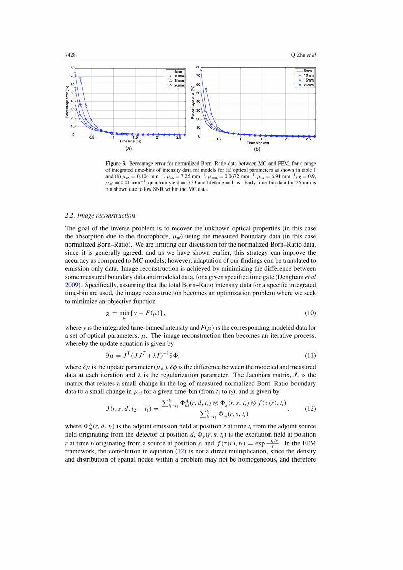
As discussed earlier, many research groups have previously presented the use of earlytime-bin intensity data for image reconstruction. It is therefore crucial to analyze the accuracyprovided by the presented FEM TD fluorescence model with respect to MC, not only as afunction of source/detector separation, but also the time-bins utilized. Figure 3(a) shows thepercentage error between simulated FEM and MC ‘normalized Born–Ratio’ data, for differentintegrated time-bins as a function of source/detector separations for the optical parametersshown in table 1. Interestingly, at the shortest source/detector separations, the percentageerror was smallest for the earliest time gates. This can be explained by the fact that at shortersource/detector distances more early photons will be detected due to a shorter mean photonpath, thus improving the statistics of the early photon gate. This is of important consideration,since most works published to date have considered a unique set of integrated time-bins for allsource/detector combinations for image reconstruction, whereas this result indicates that thebest method may also be a function of source/detector separation. In all cases, the percentageerror reduces to less than 2% for integrated time-bins of more than 1 ns.

Further models were simulated (not shown) to represent realistic bulk tissue opticalproperties of more absorption dominant organs such as the liver and spleen: μax, =0.104 mm−1, μsx = 7.25 mm−1, μam, = 0.0672 mm−1, μsm = 6.91 mm−1, g = 0.9,μaf = 0.01 mm−1, quantum yield = 0.33 and lifetime = 1 ns, which correspond to theproperties of liver at an excitation wavelength of 635 nm and emission wavelength of 660 nm.Similar trends as those shown in figures 1 and 2 were seen, with the maximum percentagedifference for intensity measurement between MC and FEM being less than 2.5% and meantime of flight less than 37 ps. The corresponding numbers for the Born–Ratio data for intensitymeasurements and mean time were found to be less than 0.45% and 22 ps, respectively.Figure 3(b) shows the percentage error between FEM and MC ‘normalized Born–Ratio’ data,for different source/detector separations, as a function of different integrated time-bins forthese higher optical parameters, displaying the same trends as those seen in figure 3(a).

7428 Q Zhu et al

(a) (b)

Figure 3. Percentage error for normalized Born–Ratio data between MC and FEM, for a rangeof integrated time-bins of intensity data for models for (a) optical parameters as shown in table 1and (b) μax = 0.104 mm−1, μsx = 7.25 mm−1, μam, = 0.0672 mm−1, μsx = 6.91 mm−1, g = 0.9,μaf, = 0.01 mm−1, quantum yield = 0.33 and lifetime = 1 ns. Early time-bin data for 26 mm isnot shown due to low SNR within the MC data.

2.2. Image reconstruction

The goal of the inverse problem is to recover the unknown optical properties (in this casethe absorption due to the fluorophore, μaf) using the measured boundary data (in this casenormalized Born–Ratio). We are limiting our discussion for the normalized Born–Ratio data,since it is generally agreed, and as we have shown earlier, this strategy can improve theaccuracy as compared to MC models; however, adaptation of our findings can be translated toemission-only data. Image reconstruction is achieved by minimizing the difference betweensome measured boundary data and modeled data, for a given specified time gate (Dehghani et al2009). Specifically, assuming that the total Born–Ratio intensity data for a specific integratedtime-bin are used, the image reconstruction becomes an optimization problem where we seekto minimize an objective function

χ = minμ

[y − F(μ)] , (10)

where y is the integrated time-binned intensity and F(μ) is the corresponding modeled data fora set of optical parameters, μ. The image reconstruction then becomes an iterative process,whereby the update equation is given by

∂μ = J T (JJ T + λI)−1∂ , (11)

where δμ is the update parameter (μaf), δφ is the difference between the modeled and measureddata at each iteration and λ is the regularization parameter. The Jacobian matrix, J, is thematrix that relates a small change in the log of measured normalized Born–Ratio boundarydata to a small change in μaf for a given time-bin (from t1 to t2), and is given by

J (r, s, d, t2 − t1) =∑t2

ti=t1 A

m(r, d, ti) ⊗ x(r, s, ti) ⊗ f (τ(r), ti)∑t2ti=t1

m(r, s, ti), (12)

where Am(r, d, ti) is the adjoint emission field at position r at time ti from the adjoint source

field originating from the detector at position d, x(r, s, ti) is the excitation field at positionr at time ti originating from a source at position s, and f (τ(r), ti) = exp −ti /τ

τ. In the FEM

framework, the convolution in equation (12) is not a direct multiplication, since the densityand distribution of spatial nodes within a problem may not be homogeneous, and therefore

A 3D FEM and image reconstruction algorithm for TD fluorescence imaging in highly scattering media 7429

Table 2. The seven regions of anatomy used within the heterogeneous mouse model, figure 1,together with chromophore concentrations and scattering properties used (Alexandrakis 2005).

Total Oxygen Water Scatter ScatterRegion hemoglobin (mM) saturation (%) concentration (%) amplitude power

Adipose 0.0033 70 50 0.98 0.53Bones 0.0049 80 15 1.4 1.47Muscles 0.07 80 50 0.14 2.82Stomach 0.01 70 80 0.97 0.97Lungs 0.15 85 85 1.7 0.53Kidneys 0.0056 75 80 1.23 1.51Liver 0.3 75 70 0.45 1.05Pancreas 0.3 75 70 0.45 1.05

the effect of associated shape functions for each spatial node and its associated neighboringnodes must be taken into account (Arridge and Schweiger 1995).

For the case of using multiple time-bin intensity data, equation (11) is simply modifiedwhereby

∂ =

⎡⎢⎢⎢⎣

∂ t2−t1

∂ t3−t2

...

∂ tn−tn−1

⎤⎥⎥⎥⎦ and J =

⎡⎢⎢⎢⎣

Jt2−t1

Jt3−t2

...

Jtn−tn−1

⎤⎥⎥⎥⎦ , (13)

where δφt2−t1 is the rate of change in measured data between time-bins t1 and t2 and Jt2−t1

is the associated Jacobian for time-bins. In the case of utilizing the Born–Ratio data, δφ inequation (11) then becomes

∂ = log

(

expm

expx

)− log

( mod

m

modx

), (14)

where the superscripts exp and mod correspond to experimental and modeled data, respectively.In order to demonstrate the capabilities of the developed image reconstruction algorithm,

together with the benefits of using early time-bins as compared to total intensity data (i.e.total integrated TPSF), a heterogeneous mouse model based on the Digimouse—figure 4(a)(Dogdas et al 2007)—has been created that consists of 46 468 nodes corresponding to 222 262linear tetrahedral elements, with optical properties as shown in table 2. Excitation (635 nm)and emission (660 nm) data were simulated using 25 sources placed directly under theabdomen, proximal to the major abdominal organs, and 25 detectors were simulated directlyon the surface above the same region: figure 4(b). For the forward model, the pancreas wasassumed to contain a fluorescence absorption of 0.002 mm−1 with a quantum efficiency of0.33 and a lifetime of 1 ns, and the TD data were modeled for a total of 3 ns at 50 ps time steps.The computational time for the forward data was 330 s using the MATLAB ParallelizationToolbox on a workstation containing six dual core Opteron 2427 processors and 16 GB ofRAM, running on eight ‘workers’.

For image reconstruction, three sets of time-bins have been considered: (1) the totalintensity from 0–0.2 ns, (2) the total intensity from 0–3 ns and (3) the total intensity from0–0.2 ns as well as the total intensity from 2–3 ns. The Jacobian for each time-bin wascalculated assuming a homogenous model consisting of purely homogenous tissue (μax =0.0115 mm−1, μam = 0.0075 mm−1, μs′x = 1.36 mm−1 and μs′m = 1.32 mm−1) and images

7430 Q Zhu et al

(a) (b)

Figure 4. (a) Heterogeneous mouse model where each region (as in table 2) is represented bydifferent colors and (b) location of the source (underneath) and detectors (above) over the abdomen.

Table 3. The expected and reconstructed peak values, FWHV of the fluorophore absorption of thepancreas in the heterogeneous mouse model, together with computation time per iteration.

Peak μaf (mm−1) FVHM (mm) Iteration time (s)

Target 0.002 7.8 –0–0.2 ns 0.000 048 30.8 1840–3 ns 0.000 056 284.3 8040–2 and 2–3 ns 0.000 052 99.4 804

were reconstructed for fluorescence absorption only, using normalized Born–Ratio data. Inall cases, to avoid the inverse crime, a second mesh consisting of 42 301 nodes correspondingto 210 161 linear tetrahedral elements was used with a regularization parameter ten timesthe maximum diagonal of the matrix JJT (see equation (11)). The corresponding images atiteration 10 are shown in figure 5 with reconstructed parameters shown in table 3.

As evident from the images shown in figure 5, reconstructed images in all cases locatedthe prostate well, with the peak reconstructed value using the ‘early’ time-bins (0–0.2 ns) =0.000 048 mm−1, using ‘early and late’ time-bins (0–0.2 and 2–3 ns) = 0.000 052 mm−1, andthe corresponding values for ‘late’ time-bins (0–3 ns) = 0.000 056 mm−1. The size of thereconstructed object was also larger for the 0–3 ns time-bins. Using either the ‘early’ or ‘earlyand late’ time-bins appears to have maintained better resolution, which is in line with previousstudies (Li and Niedre 2011, Leblond et al 2010a, Kumar et al 2006, Jin et al 2011). The lowrecovered value of the fluorophore can be due to multiple factors, with the main effect beingthe homogenous lower optical property assumption of the model. In this presented example,the whole mouse model used for reconstruction is assumed to consist of purely homogenoustissue, which inherently has a much lower optical attenuation, as compared to the model usedfor simulated data, as shown in figure 4(a).

3. Discussion

A 3D FEM implementation of the TD fluorescence light propagation in soft tissue based onthe DA has been developed and has been evaluated using both analytical and MC simulation.Using the analytical solution for the TD model based on a semi-infinite medium of givenoptical properties (table 1), the data using a 3D FEM was evaluated and shown to provide amatch with an associated error of 0.29% and 0.16% for excitation and emission intensity data,respectively, and less than 10 and 15 ps for the respective mean-time data (figure 2). Similarresults were found for varying optical parameters (not shown).

A 3D FEM and image reconstruction algorithm for TD fluorescence imaging in highly scattering media 7431

Figure 5. Target and reconstructed images for fluorophore absorption within the mouse modelpancreas using different time-bins. All reconstructed images are displayed as the threshold of 50%reconstructed peak value.

Acknowledging the fact that both the analytical and FEM solutions are based on the DA,an MC model was also utilized to provide an additional tool for the evaluation of both theFEM and the analytical solution: figures 1 and 2. TPSF data generated for both the excitationand emission light propagation from a homogenous medium (table 1) provided a good matchbetween all different simulation types (FEM, analytical and MC). As seen from figure 1,the FEM and analytical solutions did not model the early photon propagation well, owing tothe inaccuracy of the DA in this regime. Nonetheless, the overall agreement for the TPSFsbetween these three different models is found to be good in terms of the expected shape andresponses.

To provide a more quantitative evaluation of the models, the total intensity and meantime of flight were calculated for all models as a function of source–detector separation(figure 2). The largest error in the intensity data was observed between the MC modeland FEM for the smallest source–detector separation, especially in the emission data. Thiswas primarily due to the fact that the diffusion equation is not adequate for modeling theearly photons, which travel a more ballistic, i.e. non-diffuse, path. For the mean timeof flight data type, the largest error was also observed between MC and FEM; however,in this case, the emission mean time of flight showed a larger mismatch compared tothe excitation. In all models and for both data types, either for intensity or meantime of flight, the mismatch diminished as the source–detector distance was increased.Demonstrating the utility of normalizing emission data, figures 2(e) and (f) display thedifference between normalized data-sets for FEM and MC models. For both intensityand mean time of flight, the data mismatch is greatly reduced using Born normalization,supporting the use of such normalization for routine fluorescence image reconstruction

7432 Q Zhu et al

using experimental data. However, further work is needed to investigate the effect ofdifferent heterogeneous optical properties at excitation and emission wavelengths, and whethersuch normalization would still provide better information about imbedded fluorescencemarkers.

In the simulation comparison experiment, the analytical model and the FEM showedthe strongest correlation, likely because both models rely on the DA. The majordifference between these models is the type of boundary conditions employed. TheFEM employs type III boundary conditions, which have been shown to be moreaccurate than the extrapolated boundary conditions employed by the analytical model(Schweiger et al 1995).

The accuracy of integrated time-bin normalized Born–Ratio data between the FEM andMC demonstrated that for small source/detector separations the mismatch for early time-bins(<1 ns) is lower than for later arriving photon time-bins, figure 3. Although this finding maybe intuitive, it does demonstrate the need to take into account source/detector distance-specifictime-bins for imaging, using the DA, and not a globally specified early photon time-bin, toimprove the accuracy of image reconstruction.

Finally, the general framework for image reconstruction using the 3D FEM for TDtime-gated data is presented. Using a complex heterogeneous mouse model, it is shownthat early time-bin data can provide better localization and a combination of early andlate time-bins can further improve contrast as compared to total intensity data (figure 5and table 3). However the reconstructed peak values shown in this paper do not reach theexpected values, which is primarily due to the incorrect homogeneous assumption of theoptical properties within the image reconstruction. This can be further improvedby the utilization of additional reconstruction steps, whereby the background opticalproperties may be approximated using the excitation and emission data prior to fluorescencereconstruction, together with utilization of a priori structural information from dual modalitysystems (Davis et al 2007, Kepshire et al 2009).

4. Conclusion

In this paper, a 3D FEM-based diffuse TD model for NIR light transport in biological tissueis presented and validated using both analytical and MC solutions. This new functionalityallows simulation of both excitation and fluorescence TPSFs for heterogeneous scatteringand absorbing media in arbitrary geometries. The paper focused on the development of themodel and evaluations were performed theoretically via comparisons with analytical and MC.The TPSF data types presented in the comparisons include the TPSF curves for a range ofsource/detector separations, the normalized light fluence, the mean-time of photon arrival, theabsolute difference of the mean time and the percentage error between measured and simulatedintensity.

It has been demonstrated that using a 3D FEM implementation of the TD diffusion-basedlight propagation model, both the excitation and emission photon transport in a phantom canbe modeled to create time-dependent information with the lowest accuracy seen at the veryearly arriving photons. Model-based image reconstruction based on FEM implementationhas been outlined together with the utilization of multiple integrated time-bin intensity datademonstrating the benefits of incorporating early and late time-bins for the improvement ofimage accuracy.

A 3D FEM and image reconstruction algorithm for TD fluorescence imaging in highly scattering media 7433

Acknowledgments

This work has been funded by the National Institutes of Health (NIH) grants RO1 CA132750,RO1 CA120368 and K25 CA138578 through the National Cancer Institute (NCI). The TDFEM code is distributed as part of the NIRFAST modeling software at http://www.nirfast.org.

References

Alexandrakis G, Rannou F R and Chatziioannou A F 2005 Tomographic bioluminescence imaging by use of acombined optical-PET (OPET) system: a computer simulation feasibility study Phys. Med. Biol. 50 41

Arridge S R and Schweiger M 1995 Photon-measurement density functions: part 2. Finite-element-method calculationsAppl. Opt. 34 8026–37

Arridge S R, Schweiger M, Hiraoka M and Delpy D T 1993 A finite element approach for modeling photon transportin tissue Med. Phys. 20 299–309

Davis S C, Dehghani H, Wang J, Jiang S, Pogue B W and Paulsen K D 2007 Image-guided diffuse optical fluorescencetomography implemented with Laplacian-type regularization Opt. Express 15 4066–82

Dehghani H, Eames M E, Yalavarthy P K, Davis S C, Srinivasan S, Carpenter C M, Pogue B W and Paulsen K D 2008Near infrared optical tomography using NIRFAST: algorithms for numerical model and image reconstructionalgorithms Commun. Numer. Methods Eng. 25 711–32

Dehghani H, Srinivasan S, Pogue B W and Gibson A 2009 Numerical modelling and image reconstruction in diffuseoptical tomography Phil. Trans. R. Soc. A 367 3073–93

Dogdas B, Stout D, Chatziioannou A F and Leahy R M 2007 Digimouse: a 3D whole body mouse atlas from CT andcryosection data Phys. Med. Biol. 52 577–87

Ducros N, Herve L, Da Silva A, Dinten J M and Peyrin F 2009 A comprehensive study of the use of temporal momentsin time-resolved diffuse optical tomography: part I. Theoretical material Phys. Med. Biol. 54 7089–105

Fang Q and Boas D A 2009 Monte Carlo simulation of photon migration in 3D turbid media accelerated by graphicsprocessing units Opt. Express 17 20178–90

Gao F, Niu H, Zhao H and Zhang H 1998 The forward and inverse models in time-resolved optical tomographyimaging and their finite-element method solutions Image Vis. Comput. 16 703–12

Gao F, Zhao H, Tanikawa Y and Yamada Y 2006 A linear, featured-data scheme for image reconstruction in time-domain fluorescence molecular tomography Opt. Express 14 7109–24

Gao F, Zhao H and Yamada Y 2002 Improvement of image quality in diffuse optical tomography by use of fulltime-resolved data Appl. Opt. 41 778–91

Gao F, Zhao H, Zhang L, Tanikawa Y, Marjono A and Yamada Y 2008 A self-normalized, full time-resolved methodfor fluorescence diffuse optical tomography Opt. Express 16 13104–21

Gross S and Piwnica-Worms D 2006 Molecular imaging strategies for drug discovery and development Curr. Opin.Chem. Biol. 10 334–42

Hattery D, Chernomordik V, Loew M, Gannot I and Gandjbakhche A 2001 Analytical solutions for time-resolvedfluorescence lifetime imaging in a turbid medium such as tissue J. Opt. Soc. Am. A 18 1523–30

Hielscher A H, Klose A D and Hanson K M 1999 Gradient-based iterative image reconstruction scheme for time-resolved optical tomography IEEE Trans. Med. Imaging 18 262–71

Hillman E M 2002 Experimental and theoretical investigations of near infrared tomographic imaging methods andclinical applications PhD Thesis University College London

Houston S T, Jones L W and Waluch V 1988 Nuclear magnetic resonance imaging in detecting and staging prostaticcancer Urology 31 171–5

Jiang H B 1998 Frequency-domain fluorescent diffusion tomography: a finite-element-based algorithm and simulationsAppl. Opt. 37 5337–43

Jin J, Venugopal V and Intes X 2011 Monte Carlo based method for fluorescence tomographic imaging with lifetimemultiplexing using time gates Biomed. Opt. Express 2 871–86

Kepshire D, Mincu N, Hutchins M, Gruber J, Dehghani H, Hypnarowski J, Leblond F, Khayat M and Pogue B W 2009A microcomputed tomography guided fluorescence tomography system for small animal molecular imagingRev. Sci. Instrum. 90 043701

Kumar A T, Skoch J, Bacskai B J, Boas D A and Dunn A K 2005 Fluorescence-lifetime-based tomography for turbidmedia Opt. Lett. 30 3347–9

Kumar A T N, Raymond S B, Boverman G, Boas D A and Bacskai B J 2006 Time resolved fluorescence tomographyof turbid media based on lifetime contrast Opt. Express 14 12255–70

7434 Q Zhu et al

Lam S, Lesage F and Intes X 2005 Time domain fluorescent diffuse optical tomography: analytical expressions Opt.Express 13 2263–75

Leblond F, Davis S C, Valdes P A and Pogue B W 2010a Pre-clinical whole-body fluorescence imaging: review ofinstruments, methods and applications J. Photochem. Photobiol. B 98 77–94

Leblond F, Dehghani H, Kepshire D and Pogue B W 2009 Early-photon fluorescence tomography: spatial resolutionimprovements and noise stability considerations J. Opt. Soc. Am. A 26 1444–57

Leblond F, Tichauer K M and Pogue B W 2010b Singular value decomposition metrics show limitations of detectordesign in diffuse fluorescence tomography Biomed. Opt. Express 1 1514–31

Lee J and Sevick-Muraca E M 2002 Three-dimensional fluorescence enhanced optical tomography using referencedfrequency-domain photon migration measurements at emission and excitation wavelengths J. Opt. Soc. Am.A 19 759–71

Li Z and Niedre M 2011 Hybrid use of early and quasi-continuous wave photons in time-domain tomographic imagingfor improved resolution and quantitative accuracy Biomed. Opt. Express 2 665–79

Luker G D and Luker K E 2008 Optical imaging: current applications and future directions J. Nucl. Med. 49 1–4Marjono A, Yano A, Okawa S, Gao F and Yamada Y 2008 Total light approach of time-domain fluorescence diffuse

optical tomography Opt. Express 16 15268–85Massoud T F, Paulmurugan R and Gambhir S S 2004 Molecular imaging of homodimeric protein–protein interactions

in living subjects FASEB J. 18 1105–7Niedre M and Ntziachristos V 2010 Comparison of fluorescence tomographic imaging in mice with early-arriving

and quasi-continuous-wave photons Opt. Lett. 35 369–71Niedre M J, de Kleine R H, Aikawa E, Kirsch D G, Weissleder R and Ntziachristos V 2008 Early photon tomography

allows fluorescence detection of lung carcinomas and disease progression in mice in vivo Proc. Natl. Acad. Sci.USA 105 19126–31

O’Leary M A, Boas D A, Li X D, Chance B and Yodh A G 1996 Fluorescence lifetime imaging in turbid media Opt.Lett. 21 158–60

Palmedo H, Hensel J, Reinhardt M, Von Mallek D, Matthies A and Biersack H J 2002 Breast cancer imaging withPET and SPECT agents: an in vivo comparison Nucl. Med. Biol. 29 809–15

Patterson M S and Pogue B W 1994 Mathematical model for time-resolved and frequency-domain fluorescencespectroscopy in biological tissues Appl. Opt. 33 1963–74

Preisa T, Virnaua P, Paul W and Schneidera J J 2009 GPU accelerated Monte Carlo simulation of the 2D and 3DIsing model J. Comput. Phys. 228 4468–77

Riley J, Hassan M, Chernomordik V and Gandjbakhche A 2007 Choice of data types in time resolved fluorescenceenhanced diffuse optical tomography Med. Phys. 34 4890–900

Ripoll J, Nieto-Vesperinas M, Weissleder R and Ntziachristos V 2002 Fast analytical approximation for arbitrarygeometries in diffuse optical tomography Opt. Lett. 27 527–9

Rudin M and Weissleder R 2003 Molecular imaging in drug discovery and development Nat. Rev. DrugDiscov. 2 123–31

Schweiger M and Arridge S R 1995 Near-infrared imaging: photon measurement density functions Proc.SPIE 2389 366–77

Schweiger M and Arridge S R 1999 Application of temporal filters to time resolved data in optical tomography Phys.Med Biol. 44 1699–717

Schweiger M, Arridge S R, Hiroaka M and Delpy D T 1995 The finite element model for the propagation of light inscattering media: boundary and source conditions Med. Phys. 22 1779–92

Soloviev V Y, Tahir K B, McGinty J, Elson D S, Neil M A, French P M and Arridge S R 2007 Fluorescence lifetimeimaging by using time-gated data acquisition Appl. Opt. 46 7384–91

Soubret A, Ripoll J and Ntziachristos V 2005 Accuracy of fluorescent tomography in the presence of heterogeneities:study of the normalized Born ratio IEEE Trans. Med. Imaging 24 1377–86

Valim N, Brock J and Niedre M 2010 Experimental measurement of time-dependent photon scatter for diffuse opticaltomography J. Biomed. Optics 15 065006

Vishwanath K and Mycek M A 2005 Time-resolved photon migration in bi-layered tissue models Opt.Express 13 7466–82

Warner E et al 2001 Comparison of breast magnetic resonance imaging, mammography, and ultrasound forsurveillance of women at high risk for hereditary breast cancer J. Clin. Oncol. 19 3524–31

Wu J, Perelman L, Dasari R R and Feld M S 1997 Fluorescence tomographic imaging in turbid media using early-arriving photons and Laplace transforms Proc. Natl. Acad. Sci. USA 94 8783–8

Zhang L, Lee K C, Bhojani M S, Khan A P, Shilman A, Holland E C, Ross B D and Rehemtulla A 2007 Molecularimaging of Akt kinase activity Nat. Med. 13 1114–9