Embed Size (px)
Citation preview
Applying Causal-State SplittingReconstruction Algorithm to Natural
Language Processing Tasks
Tesi Doctoral - PhD Thesis
per a optar al grau deDoctora en Informatica
by
Muntsa Padro Cirera
advisor
Dr. Lluıs Padro Cirera
Ph.D. Program in Artificial IntelligenceDepartament de Llenguatges i Sistemes Informatics
Universitat Politecnica de Catalunya
Barcelona, June 2008


Al Martı, a la meva famılia i als meus amics.
Gracies per ser-hi sempre.

Abstract
This thesis is focused on the study and use of Causal State Splitting Reconstruction (CSSR)algorithm for Natural Language Processing (NLP) tasks. CSSR is an algorithm that cap-tures patterns from data building automata in the form of visible Markov Models. It isbased on the principles of Computational Mechanics and takes advantage of many proper-ties of causal state theory. One of the main advantages of CSSR with respect to MarkovModels is that it builds states containing more than one n-gram (called history in computa-tional mechanics), so the obtained automata are much smaller than the equivalent MarkovModel.
In this work, we first study the behavior of the algorithm when learning patterns relatedto NLP tasks but without performing any annotation task. This first experiments are usefulto understand the parameters that affect the algorithm and to check that it is able to capturethe patterns present in natural language sentences.
Secondly, we propose a way to apply CSSR to NLP annotation tasks. The algorithmis not originally conceived to use the hidden information necessary for annotation tasks,so we devised a way to introduce it into the system in order to obtain automata includingthis information that can be afterwards used to annotate new text. Also, some methods todeal with unseen events and a modification of the algorithm to make it more suitable forNLP tasks have been presented and tested. These three aspects conform the first line ofcontributions of this research, altogether with a deep experimental study of the proposedmethods.
The experimental study of the proposed approach is performed in three different tasks:Named Entity Recognition in general and Biomedical domain and Chunking. The obtainedresults are promising in the two first tasks though not so good for Chunking. Nevertheless,it is not easy to improve the obtained performance following the same approach, sinceCSSR needs quite reduced feature sets to build correct automaton and that limits theperformance of the developed system. For that reason, we propose to combine CSSR withgraphical models, in order to enrich the features that the system can take into account.
This combination conforms the second line of contributions of this thesis. There is avariety of possible graphical models that can be used, but for the moment we propose tocombine CSSR algorithm with Maximum Entropy (ME) models. ME models can be usedas a way of introducing more information into the system, encoding it as features. In thisline, we propose and test two methods for combining CSSR and ME models in order toimprove the results obtained with original CSSR. The first method is simple and does notmodify the automata-building algorithm while the second one is more sophisticated andbuilds automata taking into account the ME features. We will see that though much moresimpler, the first method leads to an important improvement with respect to original CSSRbut the second method does not.
Resum
Aquesta tesi es centra en l’estudi i en l’us de l’algorisme “Causal State Splitting Recon-struction (CSSR)” per tasques de Processat de Llenguatge Natural (PLN). El CSSR esun algorisme que captura els patrons d’un conjunt de dades construint automats d’estatsfinits en la forma de Models de Markov visibles. Es basa en els principis de la MecanicaComputacional tot i traient profit de les moltes propietats interessants de la teoria d’estatscausals. Un dels principals avantatges del CSSR respecte els Models de Markov es queconstrueix estats que contenen mes d’un n-gram, per tant els automats que s’obtenen sonmolt mes petits que el Model de Markov equivalent.
En aquest treball, primer de tot estudiem el comportament de l’algorisme quan l’apliquema l’aprenentatge de patrons relacionats amb tasques de PLN pero sense realitzar cap tascad’anotacio. Aquests experiments inicials ens serveixen per entendre els parametres queafecten l’algorisme i per comprovar que el CSSR pot aprendre els patrons que es troben enles frases de llenguatge natural.
Seguidament, proposem un metode per aplicar el CSSR a tasques d’anotacio de sequenciesde llenguatge natural. L’algorisme no esta originalment pensat per incloure la informaciooculta que es necessita en aquest tipus de tasques, per tant hem dissenyat un metode perintroduir-la al sistema i aixı obtenir automats que inclouen aquesta informacio i podenser usats per anotar text nou. De la mateixa manera, proposem dos metodes per trac-tar els esdeveniments no observats en les dades i una modificacio de l’algorisme que el fames apte per tasques de PLN. Aquests tres aspectes conformen la primera lınia de contribu-cions d’aquesta tesi, juntament amb un estudi experimental detallat dels metodes proposatsaplicats a diferents tasques de processat de llenguatge natural.
Aquest estudi experimental es realitza sobre tres tasques diferents: reconeixement d’enti-tats amb nom tant en un domini general com en el domini Biomedic i deteccio de sintagmes.Els resultats obtinguts son prometedors en les dues primeres tasques, pero no tan bons enl’ultima. No obstant, no es facil millorar els resultats obtinguts seguint el mateix metode,ja que el CSSR necessita tractar amb un nombre reduıt de caracterıstiques per construirautomats correctes i aixo limita la potencia del sistema, ja que no pot tractar informaciocomplicada. Per aquesta rao, proposem combinar el CSSR amb models grafics, per aixıpoder introduir informacio mes sofisticada al sistema.
Aquesta combinacio es la segona lınia de contribucions d’aquesta recerca. Hi ha diversosmodels grafics que es podrien usar, pero de moment nosaltres proposem combinar el CSSRamb models de Maxima Entropia (ME). El primer metode que proposem es el mes simplei no modifica l’algorisme de construccio de l’automat sino que nomes usa els models deME per la tasca d’anotacio. El segon metode es mes sofisticat i modifica el CSSR per talque els automats construıts tinguin en compte tota la informacio usant els models de ME.Veurem que els primer metode, tot i ser molt mes simple, aporta una millora importantdels resultats, mentre que el segon metode no aconsegueix millorar-los significativament.
Agraıments
Aquesta tesi no hauria estat possible sense l’ajuda de moltes persones a qui vull donar lesgracies. Primer de tot, vull agrair al meu germa i director Lluıs la seva ajuda, bon humori guia durant tots aquests anys. D’ell vaig aprendre, ja des de petita, el pensament crıtic iracional. Durant el meu doctorat m’ha ensenyat, a mes, que significa fer investigacio.
Tambe vull agrair a en Cosma Shalizi i la Kristina Klinkner, creadors de l’algorisme quehe utilitzat en aquesta tesi, la seva ajuda en tots els temes teorics i practics que envoltenaquest algorisme. Sense ells i les seves pacients respostes, no hauria arribat al nivell decomprensio necessari per realitzar aquest treball.
Hi ha molta mes gent a qui vull mencionar. Tinc la sort d’haver treballat en un grupon regna el bon humor i l’amabilitat. Agraeixo especialment a l’Horacio Rodrıguez elsseus desinteressats consells pel que fa a la meva recerca i a la redaccio d’aquesta tesi. Ivull mencionar amb afecte a totes les persones amb qui he compartit despatx, estones defeina, vermuts i sopars. Gracies Eli, Robert, Victoria, Luıs, Jesus, Montse, Jordi A., Xavi,Edgar, Pere, Meritxell, Maria, Dani, Roberto, Jordi P., Emili, JuanFra, Mauro i Sergi pelssomriures cada matı. I gracies tambe a la resta del grup de Processat de Llenguatge Naturalde la UPC: Jordi T., Marta, Neus, Ma Teresa, Lluıs M., Alicia, Manu, Bernardino, Nuria,Jordi D., Gerard, Javier, David, Ramon, Angels, Samir, Patrik i Carme.
Aixı mateix, vull donar les gracies a en Bill Keller per haver-me acollit durant quatremesos a la Universitat de Sussex. A ell i a en James Dowdall els agraeixo el treball que vamrealitzar junts, i a tota la gent del grup de processat de llenguatge natural de la Universitatde Sussex la seva hospitalitat.
Tambe vull expressar el meu agraıment a totes les persones que han revisat i llegitaquesta tesi. Agraeixo la seva atencio als membres del tribunal i als tres revisors anonimsque m’han fet arribar els seus comentaris sobre una versio preliminar d’aquest document.
Part de la meva recerca ha estat financada pel Comissionat per a Universitats i Recercadel Departament d’Innovacio, Universitats i Empresa de la Generalitat de Catalunya i delFons Social Europeu a traves d’una beca predoctoral FI, vinculada al projecte ALIADO(Tecnologıas del Habla y el Lenguaje para un Asistente Personal, TIC2002-04447-C02-01).Tambe m’han donat suport economic diferents projectes d’ambit europeu i estatal: CHIL(Computers In the Human Interaction Loop, IP 506909), KNOW (Desarrollo de TecnologıasMultilingues a Gran Escala para la Comprension del Lenguaje Natural), EurOpenTrad(Traduccion Automatica Avanzada de Codigo Abierto para la Integracion Europea de lasLenguas del Estado Espanyol, FIT-350401-2006-5) i HOPS (Enabling an Intelligent NaturalLanguage Based Hub for the Deployment of Advanced Semantically Enriched Multi-channelMass-scale Online Public Services, IP 507967).
Tambe vull expressar el meu agraıment a la gent de l’administracio i del laboratori decalcul del departament de LSI de la UPC que han fer possible la meva feina i estudis aquı.
En el camp personal, vull agrair profundament el seu suport i dedicar aquesta tesi atota la gent que m’ha fet costat tots aquests anys. A la meva famılia, per creure sempre enmi. A en Martı, per la seva infinita paciencia, suport i alegria, i per ajudar-me a veure lescoses clares quan tot s’enfosqueix. I als meus amics, per fer-me la vida molt mes agradable.No els puc mencionar a tots, pero es mereixen una especial atencio en Jordi, per donar-meun gran suport moral i forca de tecnic, l’Alba, per ser molt mes que una germana i estarsempre al meu costat, l’Alina, la Teresa, en Sandri, la Vir, la Montse i en Dıdac per tantacomplicitat i en Robert, en Pere, l’Anna, els tres Davids, l’Olga, en Marc i tota la gent ambqui he compartit la meva passio per tota la diversio, comprensio i felicitat.
Acknowledgments
This thesis would not have been possible without the help of many people to whom I amvery grateful. First of all, I want to thank my brother and supervisor Lluıs for his help,high spirits and guidance during all these years. From him I have learnt, since I was a smallgirl, critical and rational thinking. During my PhD he has taught me, also, the meaning ofresearch work.
I also want to thank Cosma Shalizi and Kristina Klinkner, authors of the algorithmused in this thesis, for their help in all the theoretic and practical aspects of this algorithm.Without them and their patient answers I wouldn’t have been able to understand all thenecessary details to perform this work.
There are many other people I would like to mention. I have been so lucky as to work ina group where there was always friendliness and a good atmosphere. I am specially thankfulto Horacio Rodriguez for his help during my research and the writing of this dissertation.Also, I want to mention with warm affection all the people with whom I have shared myoffice, my working time, celebrations and dinners. Thank you Eli, Robert, Victoria, Luıs,Jesus, Montse, Jordi A., Xavi, Edgar, Pere, Meritxell, Maria, Dani, Roberto, Jordi P.,Emili, JuanFra, Mauro and Sergi for your smiles every morning. And thank you also to therest of the UPC Natural Language Processing Group: Jordi T., Marta, Neus, Ma Teresa,Lluıs M., Alicia, Manu, Bernardino, Nuria, Jordi D., Gerard, Javier, David, Ramon, Angels,Samir, Patrik and Carme.
Furthermore, I am very grateful to Bill Keller for receiving me as a visiting student atthe University of Sussex for four months. I thank him and James Dowdall for the work wedid together and I also thank all the people of Natural Language Processing group of theUniversity of Sussex for their hospitality.
A special acknowledgment goes to the people that have revised and read this thesis. Isincerely thank the three anonymous reviewers that provided me with very useful feedbackabout a previous version of this thesis and the people of the thesis committee.
This research has been partially funded by the Catalan Goverment (Comissionat per aUniversitats i Recerca del Departament d’Innovacio, Universitats i Empresa de la Gener-alitat de Catalunya) through a pre-doctoral grant related to the ALIADO project (Tec-nologıas del Habla y el Lenguaje para un Asistente Personal, TIC2002-04447-C02-01).Also, some other European and Spanish projects have supported my research economi-cally: CHIL (Computers In the Human Interaction Loop, IP 506909), KNOW (Desarrollode Tecnologıas Multilingues a Gran Escala para la Comprension del Lenguaje Natural),EurOpenTrad (Traduccion Automatica Avanzada de Codigo Abierto para la IntegracionEuropea de las Lenguas del Estado Espanol, FIT-350401-2006-5) and HOPS (Enabling anIntelligent Natural Language Based Hub for the Deployment of Advanced SemanticallyEnriched Multi-channel Mass-scale Online Public Services, IP 507967).
Finally, I also want to express my gratitude to the people from the administrative andtechnical offices of the LSI department of the UPC that have made possible the years I havebeen working and studying here.
Contents
1 Introduction 1
1.1 Motivation . . . . . . . . . . . . . . . . . . . . . . . . . . . . . . . . . . . . 11.2 Overview . . . . . . . . . . . . . . . . . . . . . . . . . . . . . . . . . . . . . 21.3 Goals . . . . . . . . . . . . . . . . . . . . . . . . . . . . . . . . . . . . . . . 21.4 Structure of this Document . . . . . . . . . . . . . . . . . . . . . . . . . . . 3
2 State of the Art 5
2.1 Sequential Tasks . . . . . . . . . . . . . . . . . . . . . . . . . . . . . . . . . 52.2 Learning Sequential Models . . . . . . . . . . . . . . . . . . . . . . . . . . . 5
2.2.1 Generative Models . . . . . . . . . . . . . . . . . . . . . . . . . . . . 62.2.2 Conditional Models . . . . . . . . . . . . . . . . . . . . . . . . . . . 62.2.3 Finite State Automata . . . . . . . . . . . . . . . . . . . . . . . . . . 7
2.3 NLP Sequential Tasks . . . . . . . . . . . . . . . . . . . . . . . . . . . . . . 102.3.1 Named Entity Recognition and Classification . . . . . . . . . . . . . 102.3.2 Biomedical Named Entity Extraction . . . . . . . . . . . . . . . . . . 122.3.3 Text Chunking . . . . . . . . . . . . . . . . . . . . . . . . . . . . . . 14
3 Computational Mechanics and CSSR 15
3.1 Foundations of Computational Mechanics . . . . . . . . . . . . . . . . . . . 153.1.1 Definitions . . . . . . . . . . . . . . . . . . . . . . . . . . . . . . . . 163.1.2 Assumptions of the Theory and Limitations of Causal States . . . . 183.1.3 Summary and Important Remarks . . . . . . . . . . . . . . . . . . . 18
3.2 CSSR algorithm . . . . . . . . . . . . . . . . . . . . . . . . . . . . . . . . . 193.2.1 The Algorithm . . . . . . . . . . . . . . . . . . . . . . . . . . . . . . 193.2.2 Time and Space Complexity . . . . . . . . . . . . . . . . . . . . . . . 213.2.3 Important Issues of CSSR . . . . . . . . . . . . . . . . . . . . . . . . 21
3.3 CSSR Algorithm Step by Step . . . . . . . . . . . . . . . . . . . . . . . . . 233.3.1 The Even Process . . . . . . . . . . . . . . . . . . . . . . . . . . . . 233.3.2 The (anbn)∗ Process . . . . . . . . . . . . . . . . . . . . . . . . . . . 273.3.3 Pseudo-Even Process . . . . . . . . . . . . . . . . . . . . . . . . . . . 293.3.4 Discussion . . . . . . . . . . . . . . . . . . . . . . . . . . . . . . . . . 31
ix
x Contents
3.4 CSSR compared with other techniques . . . . . . . . . . . . . . . . . . . . . 333.4.1 ǫ-machines versus Markov Models . . . . . . . . . . . . . . . . . . . 333.4.2 ǫ-machines versus VLMM and Prediction Suffix Trees . . . . . . . . 343.4.3 CSSR versus other ǫ-machine learning algorithms. . . . . . . . . . . 34
3.5 CSSR applications . . . . . . . . . . . . . . . . . . . . . . . . . . . . . . . . 35
4 Study of CSSR Ability to Capture Language Subsequence Patterns 37
4.1 Using CSSR to Capture the Patterns of Language Subsequences . . . . . . 384.2 Capturing the Patterns of Named Entities . . . . . . . . . . . . . . . . . . . 384.3 Capturing the Patterns of Noun Phrases . . . . . . . . . . . . . . . . . . . . 41
4.3.1 Comparing Grammars to Evaluate CSSR Learning Ability . . . . . . 434.3.2 Generating Artificial Data to Study CSSR Performance . . . . . . . 45
4.4 Discussion . . . . . . . . . . . . . . . . . . . . . . . . . . . . . . . . . . . . . 474.5 Conclusions of this Chapter . . . . . . . . . . . . . . . . . . . . . . . . . . . 48
5 Adapting CSSR to Perform Annotation Tasks 49
5.1 Representing the Hidden Information . . . . . . . . . . . . . . . . . . . . . . 505.2 Learning the Automaton with the Hidden Information . . . . . . . . . . . . 50
5.2.1 An Example . . . . . . . . . . . . . . . . . . . . . . . . . . . . . . . 515.3 Using the Learned Automaton to Annotate Language Subsequences . . . . 515.4 Managing Unseen Transitions . . . . . . . . . . . . . . . . . . . . . . . . . . 535.5 Validating the Method . . . . . . . . . . . . . . . . . . . . . . . . . . . . . . 545.6 Conclusions of this Chapter . . . . . . . . . . . . . . . . . . . . . . . . . . . 55
6 Experiments and Results with CSSR in Annotation Tasks 57
6.1 Experimental Settings . . . . . . . . . . . . . . . . . . . . . . . . . . . . . . 576.1.1 Maximum Length . . . . . . . . . . . . . . . . . . . . . . . . . . . . 576.1.2 Hypothesis Test . . . . . . . . . . . . . . . . . . . . . . . . . . . . . 586.1.3 Sink Management . . . . . . . . . . . . . . . . . . . . . . . . . . . . 596.1.4 Adjusting State Deletion . . . . . . . . . . . . . . . . . . . . . . . . . 596.1.5 Synthesis . . . . . . . . . . . . . . . . . . . . . . . . . . . . . . . . . 60
6.2 Evaluation . . . . . . . . . . . . . . . . . . . . . . . . . . . . . . . . . . . . . 606.3 Named Entity Recognition . . . . . . . . . . . . . . . . . . . . . . . . . . . . 61
6.3.1 Data . . . . . . . . . . . . . . . . . . . . . . . . . . . . . . . . . . . . 616.3.2 Baseline . . . . . . . . . . . . . . . . . . . . . . . . . . . . . . . . . . 616.3.3 Alphabet . . . . . . . . . . . . . . . . . . . . . . . . . . . . . . . . . 626.3.4 Experiments and Results . . . . . . . . . . . . . . . . . . . . . . . . 626.3.5 Comparison with a Markov Model . . . . . . . . . . . . . . . . . . . 776.3.6 Discussion . . . . . . . . . . . . . . . . . . . . . . . . . . . . . . . . . 78
6.4 Biomedical Named Entity Recognition . . . . . . . . . . . . . . . . . . . . . 806.4.1 Data . . . . . . . . . . . . . . . . . . . . . . . . . . . . . . . . . . . . 806.4.2 Alphabet . . . . . . . . . . . . . . . . . . . . . . . . . . . . . . . . . 806.4.3 Experiments and Results . . . . . . . . . . . . . . . . . . . . . . . . 836.4.4 Discussion . . . . . . . . . . . . . . . . . . . . . . . . . . . . . . . . . 84
6.5 Text Chunking . . . . . . . . . . . . . . . . . . . . . . . . . . . . . . . . . . 856.5.1 Data . . . . . . . . . . . . . . . . . . . . . . . . . . . . . . . . . . . . 856.5.2 Alphabet . . . . . . . . . . . . . . . . . . . . . . . . . . . . . . . . . 85
Contents xi
6.5.3 Experiments and Results . . . . . . . . . . . . . . . . . . . . . . . . 866.5.4 Discussion . . . . . . . . . . . . . . . . . . . . . . . . . . . . . . . . . 90
6.6 Conclusions of this Chapter . . . . . . . . . . . . . . . . . . . . . . . . . . . 91
7 Extending CSSR with ME models 93
7.1 Maximum Entropy Models . . . . . . . . . . . . . . . . . . . . . . . . . . . . 947.1.1 Representing Context and Constraints . . . . . . . . . . . . . . . . . 947.1.2 Parametric Form . . . . . . . . . . . . . . . . . . . . . . . . . . . . . 95
7.2 Introducing ME models into CSSR . . . . . . . . . . . . . . . . . . . . . . . 957.2.1 Methodology . . . . . . . . . . . . . . . . . . . . . . . . . . . . . . . 967.2.2 Plain ME . . . . . . . . . . . . . . . . . . . . . . . . . . . . . . . . . 967.2.3 ME-over-CSSR . . . . . . . . . . . . . . . . . . . . . . . . . . . . . . 967.2.4 ME-CSSR . . . . . . . . . . . . . . . . . . . . . . . . . . . . . . . . . 97
7.3 Conclusions of this Chapter . . . . . . . . . . . . . . . . . . . . . . . . . . . 100
8 Experiments and Results with ME-extended CSSR 101
8.1 Data and Alphabet . . . . . . . . . . . . . . . . . . . . . . . . . . . . . . . . 1018.2 Features . . . . . . . . . . . . . . . . . . . . . . . . . . . . . . . . . . . . . . 1018.3 Experimental Results . . . . . . . . . . . . . . . . . . . . . . . . . . . . . . . 103
8.3.1 ME-CSSR in more detail . . . . . . . . . . . . . . . . . . . . . . . . 1048.3.2 Discussion . . . . . . . . . . . . . . . . . . . . . . . . . . . . . . . . . 105
8.4 Conclusions of this Chapter . . . . . . . . . . . . . . . . . . . . . . . . . . . 106
9 Conclusions and Future Directions 107
9.1 Summary and Conclusions . . . . . . . . . . . . . . . . . . . . . . . . . . . . 1079.1.1 Main Contributions . . . . . . . . . . . . . . . . . . . . . . . . . . . 1079.1.2 Related Publications . . . . . . . . . . . . . . . . . . . . . . . . . . . 110
9.2 Future Work . . . . . . . . . . . . . . . . . . . . . . . . . . . . . . . . . . . 1119.2.1 CSSR for annotation tasks . . . . . . . . . . . . . . . . . . . . . . . 1119.2.2 CSSR combined with ME models . . . . . . . . . . . . . . . . . . . . 111
Bibliography 113

CHAPTER 1
Introduction
Natural Language Processing (NLP) tasks have an intrinsic difficulty due to the fact thathuman language is very complex and ambiguous. In fact, the various kinds of ambiguity (e.g.lexical, syntactic, semantic, referential...) are one of the main problems in NLP. Solvingthose ambiguities is necessary to develop reliable tools (PoS taggers, Chunking, NamedEntity Recognizers...) that are required to build more sophisticated systems devoted toapplications such as Question Answering, Machine Translation, Information Retrieval, orSummarization among others.
1.1 Motivation
Although a Natural Language sequence may encode a semantically or pragmatically verycomplex message, it is encoded and transmitted in the form of a sequence of sounds orwords. These word sequences follow certain patterns which are usually the focus of mostof the NLP basic processors. For instance, Named Entity Recognition, Chunking, Part ofSpeech Tagging, Multi-word Expressions Detection, are tasks that depend largely on thosesequential patterns and may be approached with systems taking into account this sequentialstructure.
This thesis is focused on approaching some NLP sequential tasks within the frame-work of learning graphical models from data, more concretely, we are interested in learningProbabilistic Finite State Automata (PFSA). From the various algorithms that statisticallyinduce this kind of models, we focus on the study of a specific automata learning algorithm(CSSR) and on its applicability to some sequential NLP tasks.
We focus on this algorithm because it is similar to other algorithms successfully appliedto NLP sequential tasks, such as Markov Models or Variable length Markov Models, buthas some different properties that may be useful when learning NLP patterns, for examplethat it represents the learned patterns in the form of a PFSA.
1
2 Chapter 1. Introduction
1.2 Overview
NLP tasks can be approached using techniques based on linguistic knowledge and hand-builtrules or grammars, or can be also approached using Machine Learning (ML) techniques. Weare specially interested in the latter. Many ML techniques have been applied successfullyto various NLP tasks, but when dealing with sequential structures, it is important to useMachine Learning techniques that take into account this sequence information. According toDietterich (2002), the supervised learning algorithms may fail to learn this kind of processesbecause the training data are not drawn independently and identically as these methodsusually assume, but, as said before, the values in a sequence may influence each other.
1.3 Goals
The main focus of this work is the study and treatment of graphical models applied tosequential NLP tasks. These graphical models often model the sequences using Finite StateAutomata (FSA) or grammars. There are many approaches to this kind of tasks, some ofthe most widely used are Hidden Markov Models (HMM) or their extensions (MaximumEntropy Markov Models, Input-Output HMMs, Conditional Random Fields...). In thesemodels, language utterances are modelled as state sequences where the states represent thehidden information and the observations are modelled as emissions from these states. Oncethe way to encode the hidden information is set, the model is built by computing the variousinvolved probabilities. For example, when using a trigram HMM to perform Part of Speech(PoS) tagging, the states represent tag bigrams (one state for each possible combination oftwo PoS tags) and the emitted symbols are the words in a sentence. Then, the model istrained by computing the transition probabilities from state to state (that is, the trigramprobabilities) and the emission probabilities (probability of emitting each word being in adetermined state).
The main problem of this kind of algorithms is that the acquired graphical model hasa predefined structure, so they are not very flexible and may not adapt well to some kindsof problems. Furthermore, they suffer from data sparseness. However, there are somealgorithms that learn graphical models without predefining the structure of the problem.These algorithms are more flexible and can adapt better to each problem. Also, they canbuild better models with sparse data.
This work is focused on the study of Causal-State Splitting Reconstruction algorithm(CSSR) (Shalizi & Shalizi, 2004) and on its application to sequential NLP tasks. This algo-rithm is based on Computational Mechanics (Crutchfield, 1994) and is originally conceivedto model stationary processes by learning their causal states given data sequences. Thesecausal states build a deterministic automaton that models the process. Its main benefit isthat it builds automata in the form of Markov Models but do not need to have a predefinedstructure. Furthermore, the built models are always minimal in the sense that the automatahave always less (or equal) number of states than the equivalent Markov Model, since thecausal states join various suffixes in the same state, building a much smaller model thanthe Markov Models.
Also, another interest of using CSSR is that, since it builds minimal models, if thepattern to learn is simple enough, the obtained automaton is “intelligible”, providing anexplicit model for the training data.
Once the algorithm and its ability to learn patterns has been studied, we will present
1.4. Structure of this Document 3
an adaptation of CSSR to apply it to some NLP tasks such as text Chunking and NamedEntity Recognition both in general and medical domains. In all these tasks, the automatalearned using CSSR are used as a tool to tag new sentences. To do so, it is importantto introduce into the system knowledge about the tags taken into account, that is, aboutthe hidden information. In this work, we present a simple approach to encode this hiddeninformation into the alphabet.
1.4 Structure of this Document
The rest of this thesis is organized in the following chapters:
• Chapter 2: State of the Art.
This chapter reviews the state of the art of a variety of Machine Learning algorithms,with and special attention to algorithms for capturing sequential structures. Also,we introduce the NLP sequential tasks approached in this thesis and some systemsdevoted to those tasks.
• Chapter 3: Computational Mechanics and CSSR.
This chapter introduces the basic concepts of Computational Mechanics and the CSSRalgorithm with some simple examples of how it learns automata. Once it is presented,we compare CSSR with related techniques and we also review applications of thealgorithm in various research fields.
• Chapter 4: Study of CSSR Ability to Capture Language Subsequence
Patterns
Chapter 4 presents some experiments that we performed to study the applicabilityof CSSR algorithm in NLP tasks (Padro & Padro, 2007b). We used the algorithmto learn the patterns of language subsequences such as Named Entities and NounPhrases and studied the correctness of these patterns and the parameters that havethe largest influence on the algorithm performance. In these first experiments noannotation task was performed, the algorithm is used just to capture the patterns oflanguage subsequences.
• Chapter 5: Adapting CSSR to Perform Annotation Tasks.
This chapter introduces our proposal to use CSSR for annotating tasks (Padro &Padro, 2005a). This is one of the main contributions of this thesis. Since the algorithmis not directly prepared to introduce hidden information, we devised a method tointroduce this information into the system and use it to tag new text. Furthermore,two methods to deal with unseen events that may be found in the annotation stepare explained. Once all these contributions are introduced we present some simpleexperiments used to validate the proposed method.
• Chapter 6: Experiments and Results with CSSR in Tagging Tasks.
In this chapter, the performed experiments and the obtained results with the pro-posed method are presented and discussed. The approached tasks are: Named EntityRecognition, both in general (Padro & Padro, 2005c) and Biomedical domains (Dow-dall et al., 2007), and Text Chunking (Padro & Padro, 2005b). Studying the obtained

4 Chapter 1. Introduction
results, it is shown that one of the main error sources is the way in which CSSRdetermines the recurrent states of the automaton, that are deleted. For that reasona modification of this step of the algorithm is proposed and tested, obtaining betterresults than using original CSSR.
• Chapter 7: Extending CSSR with ME models.
This is the second main contribution of this thesis. In this chapter, we present twodifferent approaches for combining Maximum Entropy Models and CSSR (Padro &Padro, 2007a). In this way, we expect to improve the performance of CSSR alone sincewith ME models we can introduce more complicated information into the system.
• Chapter 8: Experiments and Results with ME-extended CSSR.
In this chapter, the experiments and results performed with the two extensions ofCSSR using Maximum Entropy Models are presented and discussed. These experi-ments are performed for Named Entity Recognition task.
• Chapter 9: Conclusions and Future Directions.
To conclude this work, chapter 9 reviews the main contributions and conclusions ofthis thesis as well as the main future lines that this research opens.
CHAPTER 2
State of the Art
This chapter presents a review of techniques related to Machine Learning for sequentialNLP tasks as well as automata-learning algorithms in general and CSSR in particular.Also, the tasks approached in this work and some state of the art systems devoted to themare introduced.
2.1 Sequential Tasks
We call sequential tasks those that deal with data organized as sequences, i.e. data wherethe elements have significant sequential correlation. The data concerning these kind of tasksconsist of sequences of (x, y) pairs, where x is an observation and y some hidden informationabout it (e.g. a word and its correct PoS tag, a Named Entity and its class, a word andthe tag regarding the chunk it belongs to, etc.). These (x, y) pairs will be usually relatedto other values in the sequence, where the order in which they appear is important.
We choose to focus on algorithms for extracting patterns from sequential data becausethis kind of structures are very frequent in Natural Language, since sentences are sequencesof words influencing each other. In fact, many basic NLP tasks can be regarded as sequentialtasks. Depending on the studied task, the relevant hidden information we are interested inwill be different.
Next section presents a review of different techniques that induce models from sequentialdata. We focus specially on Machine Learning (ML) techniques for learning sequentialmodels, since this is our framework and the algorithm studied in this thesis belongs to thisalgorithm class.
2.2 Learning Sequential Models
There are many different ways of representing sequential processes, and also plenty of al-gorithms for learning the different possible representations from data. We are speciallyinterested in the study of statistical graphical models for sequential tasks.
5
6 Chapter 2. State of the Art
Graphical models (Lauritzen, 1996) are often classified into two classes: directed andundirected. Undirected graphical models are those that are represented as a graph withundirected edges. Some examples are Markov Networks or Conditional Random Fields. Onthe other hand, directed graphical models are represented as directed acyclic graphs whereeach node is a random variable and the arcs represent statistical dependencies betweenthe variables. Some models belonging to this class are Hidden Markov Models or NeuralNetworks, among others. In this chapter, we will review some directed and undirectedgraphical models, with a special interest to those that also belong to the statistical modelsclass.
Statistical models can be classified as generative or discriminative models (also knownas conditional models). In next sections, we make a brief survey of different possible patternrepresentations and algorithms for learning them using this last classification.
2.2.1 Generative Models
Generative models define a joint probability distribution over observation and label se-quences p(x, y). From this joint probability, a conditional distribution can be built from agenerative model through the use of Bayes rule, though very strict independence assump-tions must be done. These models can be used to generate data or, using the conditionalprobability, to deduce the unknown class y.
Generative models have been widely used in many applications of different fields. Inthis category of algorithms there are, for example, Hidden Markov Models (Rabiner, 1990),Input-Output HMMs (IOHMM) which are HMMs for which the emission and transitiondistributions are conditional on another sequence (Bengio & Frasconi, 1995; Bengio, 1996),Generalized Hidden Markov Models that are Markov Models with the transition matricesgeneralized in such a way that they can contain any real number, so they do not representprobabilities (Upper, 1997), or Stochastic Grammars (Lari & Young, 1990). These methodshave been successfully used in a wide variety of NLP problems, not only in text processingbut also in speech recognition. See (Manning & Schutze, 1998) for an overview on theseapplications.
Nevertheless, these models have the problem that very strict independence assump-tions between observations are made when using the Bayes rule to compute the conditionaldistribution from the joint probability distribution. Furthermore, it is not practical to re-present multiple interacting features or long-range dependencies of the observations, sincethe inference problem for such models is intractable.
2.2.2 Conditional Models
The limitations that generative models introduce, due to the independence assumptionsthat must be done, make interesting to explore discriminative or conditional models. Thesemodels are used for modeling the conditional probability of an unobserved variable y on anobserved variable x, p(y|x). This probability can be used for predicting y from x withouthaving to use Bayes rule and the consequent independence assumptions. On the otherhand, conditional models, differently from generative models, do not allow the generationof samples.
In this section, we focus on graphical conditional models, though there are also con-ditional models that do not have a graphical representation, such as Maximum EntropyModels (Berger et al., 1996; Ratnaparkhi, 1997).
2.2. Learning Sequential Models 7
This kind of conditional models are non-generative finite-state models based on next-state classifiers that specify the probabilities of possible label sequences given an observationsequence. These models can take into account the possible dependency of the transitionprobability between labels with not only the current but also with other observations.The independence assumption of generative models does not allow this. Some examplesof conditional models are Maximum Entropy Markov Models (MEMMs) (McCallum et al.,2000), discriminative Markov Models (Bottou, 1991) and Conditional Random Fields (CRF)(Lafferty et al., 2001). In fact, CRFs perform better and avoid some MEMMs limitationsin many experiments performed by Lafferty et al. (2001).
All the models mentioned above, both generative and conditional, have the limitationthat the structure of the model has to be previously determined, they make strong as-sumptions about the nature of the data-generating process. Conditional models have thebenefit that extra features can be introduced which can give more information to the sys-tem. Nevertheless, the only information acquired from the training set are the probabilitydistributions for the models. For that reason, we are interested in studying those algorithmsthat learn finite state automata (FSA) from data. Though FSAs are a subset of generativemodels, we are interested in studying them separately because the algorithm studied in thiswork belongs to this class. Furthermore, this kind of representation has the benefit thatit is not necessary to pre-set the structure of the graphical model so it is interesting todistinguish it from other generative models such as Markov Models.
2.2.3 Finite State Automata
There is a wide range of finite state automata, as well as of automata-learning algorithms.Vidal et al. (2005a; 2005b) present a survey of different FSAs with a detailed theoret-ical study. Here we will summarize some of the possible FSA representations and somealgorithms to learn them.
A Finite State Automaton is a model of behavior consisting of a finite set of states,an input alphabet, and a transition function that maps input symbols and current statesto a next state. It also may have an initial state and a set of final states. Each statestores information about the past, i.e. it reflects the input changes from the system start tothe present moment. The automaton evolutes from one state to another depending on thetransition function. A transition indicates a state change and is labeled with an alphabetsymbol. Furthermore, each transition can have an assigned probability, in this case wewill say that the automaton is probabilistic (PFSA). If there is only one possible transitionfor each state with each symbol, the automaton is said to be deterministic, since there isonly one possible future state given the current state and the transition symbol. When wetalk about FSA, we will refer to deterministic automata. If being in a determined statethere is more than one state receiving a transition with a given symbol, the automata isindeterministic.
Non-statistical Automata Inference
A first group of automata learning algorithms consist of algorithms that infer automatavia non-statistical learning. Under this group, we will distinguish between algorithms thatlearn non-probabilistic automata from those that learn probabilistic automata.
One of the algorithms that learn non-probabilistic automata via non-statistical learningis RPNI (Regular Positive and Negative Inference) (Oncina & Garcia, 1991; Garcia et al.,
8 Chapter 2. State of the Art
2000) that infers regular languages from positive and negative examples. Another exampleis the one proposed by Trakhtenbrot and Barzdin (1973) and applied to grammatical in-ference by Gold (1978). Other algorithms of this kind are Error Correction GrammaticalInference (ECGI) (Rulot & Vidal, 1987; Rulot, 1992), which is a heuristic that incremen-tally constructs a regular grammar from a positive sample set, and Grammatical Inferencemethods based on morphic generators (Garcia et al., 1987; Segarra, 1993) that recognizea specific class of languages (the local languages) but allow the incorporation of a priory
knowledge.Regarding the algorithms that build rules or automata in a non-statistical way but use
some statistics to weight the rules or the transitions in an automaton, for example ECGIgrammars can be extended introducing statistical information about the usage probabilityfor each rule. There are different ways to do so (N.Prieto, 1995; Rulot, 1992), one of theseextensions is named extended ECGI (ECGIE) (Pla, 2000). Another possibility is to estimatethe probabilities of context-free rules to build Stochastic Context Free Grammars (SCFG)(Baker, 1979; Lari & Young, 1991).
Statistical Automata Inference
Finally, there are the reconstruction algorithms that build statistical automata, inferringboth architecture and parameters, using different techniques. This kind of algorithms aremore flexible and are expected to be better for complex NLP tasks where a big amount ofdata would be necessary to learn the automaton that represents (or approximates) them.
Some algorithms in this class are those that build Variable-Length Markov Models(VLMM). To construct VLMM from sequential data, the “context” algorithm (Rissanen,1983) and its descendants (Buhlmann & Wyner, 1999; Willems et al., 1995; Tino & Dorner,2001) can be used. In fact, these algorithms are related to causal state reconstruction algo-rithms (discussed below), being actually included as a special case of them (Shalizi et al.,2002).
The power of VLMM is that the constructed models take into account histories ofdifferent lengths depending on their relevance, which does not happen in traditional HMMs.This is a strength of those models, since they can use long suffixes when necessary withoutstudying all suffixes of that length, what will be computationally very expensive.
VLMMs have been successfully used for example in speech recognition (Nadas, 1984;Jelinek, 1990)
Methods related to VLMMs are those that build Prediction Suffix Trees (PST) (Ronet al., 1994a; Ron et al., 1994b) since it is always possible to transform a PST into a FiniteState Automaton. A PST is an extension of Suffix Trees (Galil & Giancarlo, 1988) thatintroduces probabilities in the edges and states. PST is a tree where each node has a pair (s,γs) where s is a string (drawn from an alphabet Σ) associated to the walk starting at thatnode and ending in the root of the tree, and γs is the next symbol probability distributionfor string s. From each node there is at most one outgoing edge labeled with each symbol.A walk on the underlying graph of the automaton always ends in a state labeled by a suffixof the sequence. Ron et al. (1994a; 1994b) propose an algorithm to implement a variablelength model expanding only the tree branches that add statistically different informationthat the shorter suffixes.
PSTs have been used in NLP field to learn the structure of English to be used to correctcorrupted texts (Ron et al., 1994b) and to tasks such as Part of Speech tagging (Schutze
2.2. Learning Sequential Models 9
& Singer, 1994). Similar tree machines were presented in (Rissanen, 1983) and applied touniversal data compression (Weinberger et al., 1992; Weinberger et al., 1995)
A recent extension of PSTs are Looping Prediction Suffix Trees (Holmes & Isbell, 2006)which is centered on inferring hidden state when the environment takes the form of aPartially Observable Markov Decision Process.
There are also Utile Suffix Memory (USM) algorithm and its extension UTree (Mc-Callum, 1995b; McCallum, 1995a) that are very similar to VLMM learning methods butwith a reward-based stopping criterion that expands a child node only if the distribution ofnext-step reward appears to differ statistically significantly from that of its parent.
ǫ-machines Inference
Another group of algorithms for statistical automata inference, in which we are speciallyinterested, are those that build ǫ-machines. ǫ-machines are statistical automata formed bythe causal states of a process. The causal states of a process are sets of suffixes that havethe same probability distribution for the future. They are very powerful and have manydesirable properties, as will be introduced in chapter 3. According to (Shalizi & Shalizi,2004), VLMM are a particular case of ǫ-machines, under restrictive and generally under-appreciated assumptions. In fact, causal state methods have some advantages over VLMMmethods, beginning with that they are more widely applicable. Furthermore, VLMM aregenerally more complicated than ǫ-machines.
To build ǫ-machines, there are different kinds of algorithms. On the one hand there areState-Merging ǫ-Machine Inference Algorithms that use what one might call state compres-sion or merging. The initial assumption of these algorithms is that each distinct historyencountered in the data is a distinct causal state. Histories are then successively mergedinto causal states when their morphs are close enough. These algorithms can learn HMMs(Stolcke & Omohundro, 1993) and finite automata (Trakhtenbrot & Barzdin, 1973; Mur-phy, 1996). Some algorithms in this group are, for example, subtree-merging algorithm(Crutchfield & Young, 1989; Crutchfield & Young, 1990; Hanson, 1993; Crutchfield, 1994)and “topological” merging procedure (Perry & Binder, 1999).
On the other hand, there is the algorithm used in this work, Causal-State SplittingReconstruction (CSSR) (Shalizi & Shalizi, 2004), also belonging to ǫ-machine inferencealgorithm class. It induces deterministic automata from sequential data by inferring thecausal states of the process (see chapter 3 for details).
Compared to other algorithms for automata learning such as ECGI (or ECGIE), CSSRhas the advantage that the learned automata do not depend on the order the sequencesappear in the training data and that it is more general because it infers the causal statesof processes by studying the future probability distribution for each suffix, so it generalizesthe pattern of the sequence using suffix information instead of creating a pattern for eachoccurrence. Also, since it builds the automaton using statistical information, it is expectedto capture better the behavior of the process.
Chapter 3 will introduce the concepts of Computational Mechanics and the CSSR al-gorithm. Once that has been presented, a more detailed discussion about the similaritiesand differences specially between CSSR and VLMM and Suffix Trees will be performed.Also the algorithm used in this work will be compared with other algorithms that learnǫ-machines.
10 Chapter 2. State of the Art
2.3 NLP Sequential Tasks
As we have said in section 2.1, this work is focused on studying the applicability of CSSRalgorithm to NLP sequential tasks. In this section, the tasks under consideration in thiswork (Named Entity Recognition in general and Biomedical domains and Text Chunking)are briefly presented.
There are other NLP tasks that may be interesting to approach with CSSR algorithm.For example, one task that we are planning to study in the future is Part of Speech tag-ging. Nevertheless, for the moment we focus on tasks that imply detecting subsequences ofwords in a sentence, since in this case the hidden information is much simpler. To mark asubsequence as a Named Entity (NE) or a chunk, we need just three tags marking if a wordis at the beginning of a subsequence, at the end of it or neither of those, or alternativelywe can mark if a word is at the beginning, inside or outside an NE. Apart from that wewill need the information about which kind of subsequence is it (type of chunk or NE), butin our approach we first perform the recognition of the subsequence. If we want to applyCSSR to PoS tagging, for example, or to other tasks that have more possible hidden tags,it is not possible to use the approach we propose in this work, so other methods have to beexplored.
2.3.1 Named Entity Recognition and Classification
Named Entity Recognition and Classification (NERC) task, also known as Named EntityExtraction (NEE), consists of detecting lexical units in a word sequence, referring to concreteentities and of determining which kind of entity the unit is referring to (persons, locations,organizations, etc.). This information is used in many NLP applications such as QuestionAnswering, Information Retrieval, Summarization, Machine Translation, Topic Detectionand Tracking, etc. The more accurate the extraction of Named Entities is, the better theperformance of the system will be.
NERC consists in two steps that could be approached either sequentially or in parallel.The first step is Named Entity Recognition (NER) which consists of detecting which parts ofa text belong to an NE. The second step is Named Entity Classification (NEC) that consistsof classifying the NEs into a set of predefined classes (person, location, organization, etc).
Though first systems related to this task date from 1991 (Rau, 1991) the concept ofNamed Entity was introduced in 1996 within the framework of the Sixth Message Un-derstanding Conference (MUC-6) (Grishman & Sundheim, 1996), devoted to InformationExtraction, that included for the first time an NERC task.
After the introduction of this important task, many other conferences included sharedtasks and workshops devoted to NERC. Some examples are HUB-4 (Chinchor et al., 1998),MUC-7 and MET-2 (Chinchor, 1998), IREX (Sekine & Isahara, 2000), CoNLL-2002 (TjongKim Sang, 2002a) and CoNLL-2003 (Tjong Kim Sang & De Meulder, 2003) shared tasks,ACE (Doddington et al., 2004) and HAREM (Santos et al., 2006).
Framed in these and other conferences, several approaches to Named Entity Recognitionand Classification task can be found. Nadeau and Sekine (2007) present a complete survey ofsome of NERC techniques and of the most used features and evaluation methods. Anotherinteresting survey on a variety of Named Entity Recognition and Classification approachesis presented by Mansouri et al. (2008a).
In next sections we will mention some of these systems dividing them into three classes:
2.3. NLP Sequential Tasks 11
hand-made or knowledge-based systems, supervised learning systems and semi-supervisedand unsupervised methods.
Knowledge-Based Systems
This kind of method was specially used at the beginning of the research in NERC systems.These approaches have typically used manually constructed finite state patterns, or rulesets. Some examples of those systems are found in MUC-6 and MUC-7 conferences or insubsequent related work (Appelt et al., 1995; Weischedel, 1995; Krupka & Hausman, 1998;Humphreys et al., 1998; Black et al., 1998; Aone et al., 1998; Mikheev et al., 1998; Mikheevet al., 1999) for English NERC. More recently, Budi and Bressan (2003) propose an NERCmethod based on association rules, a technique widely used in data mining field.
The performance obtained with such systems is usually high, however, rule-based ap-proaches lack the ability of coping with the problems of robustness and portability. Fur-thermore they need a great human effort to adapt to each new language.
Supervised Learning Systems
Supervised Learning techniques are currently the most widely used for NERC task. Firstapproaches include the use of variants of Hidden Markov Models (Bikel et al., 1997), DecisionTrees (Sekine, 1998), Maximum Entropy Models (Borthwick et al., 1998; Borthwick, 1999)or a variant of Brill (1995) transformation-based rules (Aberdeen et al., 1995). Besides,some hybrid approaches combining machine learning techniques with gazetteer informationor hand-made rules were tested in MUC-7 conference (Yu et al., 1998; Borthwick et al.,1998; Mikheev et al., 1998) .
More recent supervised approaches to NERC task were framed in CoNLL-2002 (TjongKim Sang, 2002a) and CoNLL-2003 (Tjong Kim Sang & De Meulder, 2003) shared tasks.Both tasks consisted of detecting and classifying NEs, on texts written in different languages.All the participant systems used Supervised or Semi-Supervised Learning approaches.
Some examples of supervised methods used for NERC presented both in these andother conferences are Support Vector Machines (McNamee & Mayfield, 2002; Mayfieldet al., 2003; Asahara & Matsumoto, 2003; Mansouri et al., 2008b), decision trees (Black &Vasilakopoulos, 2002), transformation-based learning (Black & Vasilakopoulos, 2002; Flo-rian et al., 2003), Hidden Markov Models (usually combined with other systems) (Jansche,2002; Burger et al., 2002; Malouf, 2002a; Zhou & Su, 2002; Florian et al., 2003; Klein et al.,2003; Mayfield et al., 2003; Whitelaw & Patrick, 2003), Maximum Entropy Models (Malouf,2002a; Chieu & Ng, 2002; Chieu & Ng, 2003; Bender et al., 2003; Curran & Clark, 2003;Florian et al., 2003; Klein et al., 2003), memory-based learning (Tjong Kim Sang, 2002b;Cucerzan & Yarowsky, 2002; Meulder & Daelemans, 2003; Hendrickx & van den Bosch,2003), AdaBoost (Carreras et al., 2002; Tsukamoto et al., 2002; Wu et al., 2002; Carreraset al., 2003b; Wu et al., 2003), Winnow techniques (Zhang & Johnson, 2003; Florian et al.,2003), perceptrons (Carreras et al., 2003a), Conditional Random Fields (McCallum & Li,2003), neural networks (Hammerton, 2003) and combination of various methods (Florian,2002; Florian et al., 2003; Klein et al., 2003; Mayfield et al., 2003; Wu et al., 2003; Munroet al., 2003).
The problem with Supervised Learning techniques is that large amount of tagged dataare necessary to develop accurate systems. Obtaining these data may be very difficult andexpensive, specially in the case of minority languages. For that reason, in last years systemsusing semi-supervised and unsupervised techniques have been developed.
12 Chapter 2. State of the Art
Semi-Supervised and Unsupervised Systems
Semi-supervised methods are those that need some annotated data to learn a first classifierand then improve this classifier using not-annotated data. These methods are speciallyuseful when dealing with tasks or languages with small amount of available data. Here wemention some approaches to NERC task with semi-supervised learning techniques.
Collins and Singer (1999) parse a complete corpus in search of candidate NE patterns.They use the output of a PoS tagger that can mark proper names and also lexical andsyntactic information. Another idea is to learn several types of NE simultaneously whatallows the finding of negative evidence and reduces over-generation (Cucerzan & Yarowsky,1999; Collins, 2002).
One of the most widely used semi-supervised technique is bootstrapping (Riloff & Jones,1999; Cucchiarelli & Velardi, 2001). Some of these systems use hand annotated seeds andothers use the output of existing NERC systems to start the learning of their classifier.
In (Ando & Zhang, 2005) a semi-supervised method based on structural learning calledSVD-ASO is presented and applied to NERC and Chunkhing tasks obtaining a high per-formance.
Ji and Grishman (2006) show that an existing NE classifier can be improved usingbootstrapping methods. They demonstrate that relying upon large collection of documentsis not sufficient by itself. Selection of documents using information retrieval-like relevancemeasures and selection of specific contexts that are rich in proper names and coreferencesbring the best results in their experiments.
Regarding unsupervised learning methods, typical approaches use clustering, lexicalresources, lexical patterns or statistics computed on a large unannotated corpus. Someexamples are the use of WordNet and topic signatures (Alfonseca & Manandhar, 2002),the identification of hypernyms using the web Evans (2003) or the counting of the numberof occurrences of passages that usually precede NEs (Cimiano & Volker, 2005). Also,(Shinyama & Sekine, 2004) present the use of the fact that Named Entities appear, moreoften than common names, at the same time and related to the same topics in multiple newssources. Etzioni et al. (2005) use Pointwise Mutual Information and Information Retrievalas a feature to assess that an NE can be classified under a given type. In (Kim et al., 2002)a combination of three learning systems (Maximum Entropy, memory-based learning andsparse network of Winnows) is used to build an unsupervised learning model that uses asseeds a small-scale named entity dictionary.
2.3.2 Biomedical Named Entity Extraction
Named Entity (NE) Extraction in medical texts consists of identifying the medical termsof a text and classifying them into different classes.
The ability to extract sequences from a document collection that convey domain specificmeaning not only provides the raw material for the creation of domain specific thesauri andontologies (Sanjuan et al., 2005), but also represents a crucial preprocessing stage for NLPapplications that operate over specialized domains (Weeds et al., 2005). However, termi-nology extraction still remains a challenging task to which statistical, linguistic and hybridalgorithms have all been applied with their differing levels of computational complexity andsuccess rates (Castellvı et al., 2001).
This extraction task is complicated by two factors. First, the flexibility with which aterm can be defined leads to many competing and sometimes incompatible notions of what
2.3. NLP Sequential Tasks 13
constitutes a term in a particular field. Broadly the definitions range from statisticallysignificant sequences (Spasic et al., 2005) to specific syntactic phrasal groupings (minimalor fully project noun phrases and coordinated conjunctions involving ellipsis) (Jacquemin& Bourigault, 2003). However, while the exact definition is flexible it is not arbitrary, butresults directly from the application to which the terms will be employed (Cabre et al.,2005; L’Homme et al., 2003). For example, in constructing a domain specific thesaurusit would be useful to extract the embedded term “NF-kappa B” from the second term insentence 2.1. However, as a preprocessing stage for further document analysis (such as inQuestion Answering (Rinaldi et al., 2004a; Rinaldi et al., 2004b)) the complete minimal NP“NF-kappa B activation” is more useful.
The second complicating factor is the level of semantic granularity required for a se-quence to be considered a domain specific term. While the name of an organization willalways be considered a Named Entity regardless of where it appears, terms are inextricablylinked to the corpus they appear in. For example, in sentence 2.1 the phrase “reactive oxy-gen production” is not considered a term from this domain since it is not specific enough.Given a different document collection, with a different domain of focus this same sequencemay well be marked as terminological.
(2.1) IL-2 gene expression and NF-kappa B activation through CD28 requiresreactive oxygen production by 5-lipoxygenase
These factors have lead to much success in measuring domain specificity through corpusanalysis and a growing understanding of the different features useful in extracting termi-nology.
There are many different approaches to this task. For example, the least domain-specific methods for term extraction use weighted document frequency counts to measurethe probable importance of terms in the domain e.g. C/NC techniques (Spasic et al., 2005).Other approaches are based in corpus frequencies, such as a system that performs a corpuscomparison using the range and frequency of word forms (Chung, 2003) or the systemdeveloped by Nakagawa and Mori (2003) based on the statistics about the relation betweena compound noun and its constituents that are simple nouns.
Other state of the art methods can be found in the framework of the shared task atBioNLP/NLPBA 2004 (Kim et al., 2004) that was devoted to Bio-Entity Recognition Task.In this task, the system that performed best (GuoDong & Jian, 2004) combined HMM andSVM with features specially defined for the task and the second one (Finkel et al., 2004)used Maximum Entropy Markov Models combined also with gazetteers and web resources.
A much simpler approach has been proposed by Ponomareva et al. (2007a), that usesan HMM with poor knowledge obtaining very competitive results. In (Ponomareva et al.,2007b) also a comparison between HMMs and Conditional Random Fields applied to thistask is performed.
All this methods perform both recognition and classification of Biomedical NEs. Asfor NER in general domain, in this thesis we will only approach the recognition task.There are some systems that also perform this task separately, to which we will be ableto compare our results. On the one hand, there is the system of Lin et al. (2004) thatuses Maximum Entropy Models, and some post-processing techniques to expand the limitsof NEs depending on the boundary words. On the other hand, another system combiningSVMs (Lee et al., 2004) and some post-processing techniques to extend the boundaries ofNEs based in dictionaries is also comparable to our work.
14 Chapter 2. State of the Art
2.3.3 Text Chunking
Text Chunking consists of dividing sentences into non-recursive non-overlapping phrases(chunks) and of classifying them into a closed set of grammatical classes (Abney, 1991) suchas noun phrase, verb phrase, etc. Each chunk contains a set of correlative, syntacticallyrelated words
This task is usually seen as a preparatory step in full parsing, but in fact, for manyNLP tasks, having the text correctly separated into chunks is preferred than having a fullparse tree, more likely to contain mistakes. In fact, sometimes the only information neededare the noun phrase (NP) chunks, or, at most, the NP and VP (verb phrase) chunks. Forthat reason, the first efforts devoted to Chunking were focused on NP-chunking (Church,1988; Ramshaw & Marcus, 1995), others deal with NP, VP and PP (prepositional phrase)(Veenstra, 1999). In (Buchholz et al., 1999) a complete approach to perform text Chunkingfor NP, VP, PP, ADJP (adjective phrases) and ADVP (adverbial phrases) using Memory-Based Learning is presented.
As most NLP tasks, Chunking can be approached using hand-built grammars and finitestate techniques or via statistical models and Machine Learning techniques. Some of theseapproaches are framed in the CoNLL-2000 Shared Task (Tjong Kim Sang & Buchholz,2000).
Three participant systems of this shared task used rule-based systems (Vilain & Day,2000; Johansson, 2000; Dejean, 2000), one was implemented using memory-based systems(Veenstra & van den Bosch, 2000) and most participants used statistical systems. Thestatistical techniques used were maximum entropy based methods (Osborne, 2000; Koeling,2000) and Markov Models related methods (Pla et al., 2000; Zhou et al., 2000). Finally,the best systems used system combination. Tjong Kim Sang (2000) trained and tested fivememory-based learning systems and then combined them buy majority voting. van Halteren(2000) used Weighted Probability Distribution Voting (WPDV) for combining the results offour WPDV chunkers and a memory-based system. Kudo and Matsumoto (2000) presenteda combination with a dynamic programing algorithm of 231 support vector machines. Animprovement of this system was presented in (Kudo & Matsumoto, 2001).
Posterior systems related to CoNLL-2000 shared task are, for example, (Zhang et al.,2001; Zhang et al., 2002) that use Winnow-related methods and (Carreras & Marquez,2003) that uses a perceptrons. Another interesting approach is presented by Thollard andClark (2002), where Probabilistic Suffix Trees are applied to Chunking task. The data usedin that work is the same as used in CoNLL-2000, so all results can be compared.
The semi-supervised method presented by Ando and Zhang (2005), already introducedin section 2.3.1, also obtains good results in chunking task using the CoNLL-2000 data.
Wu et al. (2006) and Lee and Wu (2007) present a general, multi-lingual phrase chunk-ing system based on combining Support Vector Machines with a masking method thatintroduces a significant improvement of the obtained performance.
Regarding chunking systems devoted to less common languages, an interesting approachfor the Korean is presented in (Park & Zhang, 2003). This approach combines a set of hand-written rules with a memory-based learning method that corrects some of the errors of therule-based system. For Chinese, Li et al. (2003b) present a chunker based on MaximumEntropy Models, Li et al. (2003a) a system based on HMMs and Li et al. (2004) one thatuses support vector machines.
CHAPTER 3
Computational Mechanics and CSSR
This chapter introduces the theoretical foundations of Computational Mechanics (CM) ne-cessary to understand the CSSR algorithm and presents the algorithm itself.
Section 3.1 introduces the basic concepts of Computational Mechanics, 3.2 presents theCSSR algorithm with its main issues summarized in section 3.2.3, section 3.4 discusses thedifferences between CSSR and the similar algorithms already mentioned in 2.2 and section3.5 overviews some other applications of CSSR algorithm either related to NLP tasks ornot. For some examples of how CSSR learns automata from sequential data and discussionabout some interesting issues of the algorithm, see Appendix 3.3.
3.1 Foundations of Computational Mechanics
Since various research fields require models of observed processes, there is an importantinterest on finding the best way to extract patterns from data. Some examples could be timeseries analysis, decision theory or machine learning. Computational mechanics, as definedin (Crutchfield, 1994) aims to understand the nature of patterns and pattern discovery.From either empirical data or from a probabilistic description of a determined behavior,it tries to infer a model of the hidden process that generated the observed behavior. Thisrepresentation captures the patterns of the process reflecting its causal structure what isuseful to predict future behavior. The goal of computational mechanics is to find a predictorof maximum strength and minimum complexity.
In fact, computational mechanics goes further than what is usually called pattern recog-nition in the field of computer science. It is not only concerned about learning the patternsbut also about which is the best way to represent them.
This chapter introduces the basic theoretical ideas related to the part of computationalmechanics we are interested in. These are necessary concepts to introduce the algorithmused in this work.
15
16 Chapter 3. Computational Mechanics and CSSR
3.1.1 Definitions
Next sections define some important concepts of computational mechanics. For these def-initions, we use the convention of using capital letters to denote random variables andlower-case letters for their particular values. For more details see (Shalizi & Crutchfield,2001) or (Crutchfield, 1994).
Process, History and Future
A process is a sequence of random variables (Ai) taking values from a discrete alphabet Σdetermined by a given probability distribution. Thus, a process is a sequence with the formA0, A1, A2, ..., AT .
Given a process, we can define a history or past of length L (XLi ) as any subsequence
of finite length L preceding the ith element (XLi = Ai−(L−1), Ai−(L−2), ..., Ai−1). Given
a history, it is possible to determine the probability of each possible following sequence,called future (ZL
i ) determined by the probability distribution of the process. A future is thesequence of length L following (and including) the ith symbol: ZL
i = Ai, Ai+1, ..., Ai+L−1.We say that a process is stationary if and only if the probability of seeing any subse-
quence is time invariant, so if it does not depend on the index i. This is equivalent to saythat P (ZL
i = zL) = P (ZL0 = zL) for all possible i and L.
From now on, we will consider stationary processes, so we will ignore the index i andrefer to histories and futures as XL and ZL, or more generally as X− and Z+. Then, ourgoal is to predict all or part of the future Z+ using some function of some part of the pastX−.
Equivalent Histories and Causal States
Given a concrete history x− there is a determined probability distribution of seeing a fu-ture Z+ after this history: P (Z+|x−). Two histories, x− and y−, are equivalent whenP (Z+|x−) = P (Z+|y−), i.e. when they have the same probability distribution for thefuture.
The different future distributions build the equivalence classes that are defined by afunction ǫ:
ǫ(y−) ≡ {x− | P (Z+|x−) = P (Z+|y−)}
Those equivalence classes are groups of histories sharing future distributions and arenamed causal states of the process.
Each causal state si has the following information associated:
1. The label (i) of the state.
2. The set of histories belonging to this state.
3. The future probability distribution P (Z+|si), that is equal to P (Z+|x−) for all histo-ries x− belonging to this state si.
Causal states have many desirable properties that make them the best possible repre-sentation of a process. Some of the main properties are that they are minimal (in the sensethat any other representation of the process with equivalent predicting power will be morecomplex) and have sufficient statistics to represent a process, this is, from causal states it
3.1. Foundations of Computational Mechanics 17
is possible to determine the future for a given past, so they define correctly and minimallya process. These, and other properties and theorems are proven in (Shalizi & Crutchfield,2001). Here we summarize the main conclusions and properties:
• Causal states are maximally accurate predictors of minimal statistical complexitywhat makes them the best possible representation of the patterns of a process.
• Causal states are as good at predicting the future as complete histories.
• The causal states of a process are sufficient statistics for predicting it.
• Causal states are minimal, so any other representation of the process, which is as goodas predicting the observations as the causal states, will be more complex
• Causal states are unique
• The causal states of a process form a deterministic machine and are recursively cal-culable.
• A process’s causal states are the largest subsets of histories that are strictly homoge-neous with respect to futures of all lengths1.
Causal State to State Transitions and ǫ-machines
At any given time, the current causal state and the next observed value in the sequencedetermine the next causal state. Furthermore, given the current causal state, all the possiblenext values of the future (Z+) have well defined conditional probabilities. Thus, given a setof causal states representing a process and their future distribution probabilities, we candefine a state-to-state transition matrix (Tij(a)) for each symbol a, that gives the probabilityof making the transition from state si to state sj with a determined symbol a.
Also, we can define a machine that combines the set of causal states and the transitionmatrix Tij(a) that represents the process. This machine is called ǫ-machine (Crutchfield,1994; Upper, 1997). The ǫ-machine is thus a causal representation of all the patterns of theprocess. Furthermore, it is maximally predictive and minimally complex as causal statesare. Here we summarize the most important properties of ǫ-machines:
• ǫ-machines are deterministic so, given a state si and a symbol a there is at most onestate sj receiving the transition from state si with this symbol. This implies that forevery history x− ∈ si the history x−a is a history of state sj.
• ǫ-machines are markovian, what means that the causal state at time t is determinedby the state in time t−1, being independent of the previous causal states. This gives abasis to the claim that the causal states can be considered a generalization of Marko-vian states tough, in fact, ǫ-machines have richer properties than Markov processes(Kemeny & Snell, 1976; Kemeny et al., 1976), as will be argued in section 3.4.1.
ǫ-machine Reconstruction
ǫ-machine reconstruction is any procedure that given a process produces the ǫ-machine thatrepresents it.
1A set X is strictly homogeneous with respect to a random variable Y when the conditional distributionP (Y |X) for Y is the same for all measurable subsets of X.
18 Chapter 3. Computational Mechanics and CSSR
ǫ-machines can be analytically calculated from given distributions or systematically ap-proached from empirical data. In the first case, a mathematical description of the processis needed. In the second case, the only evidence of the process available are some datasequences and it would be necessary to empirically estimate the probability distributionof the process. There are plenty of algorithms that performs this estimation and the re-construction of the ǫ-machine from them. Some, such as those used in (Crutchfield, 1994;Crutchfield & Young, 1990; Crutchfield & Young, 1989; Hanson, 1993) take the raw dataas a whole and produce the ǫ-machine. Others, as the one used in this work, could op-erate incrementally, taking individual measurements and re-estimating the set of causalstates and their transition probabilities. See section 2.2 for more algorithms on ǫ-machinereconstruction.
3.1.2 Assumptions of the Theory and Limitations of Causal States
All we have presented can be formally proven if some restrictive assumptions are made(Shalizi & Crutchfield, 2001; Crutchfield, 1994). Here we summarize these assumptions:
• The observed process is formed by sequences of discrete symbols from a closed alpha-bet, so it will not be valid for processes with continuous variables.
• The process is discrete in time.
• The process is a pure time series, e.g. without spatial extent.
• The observed process is stationary.
• Prediction can only be based on the process’ past, not on any outside source ofinformation.
These assumptions are necessary to prove the theorems and lemmas behind causal statetheory but there are methods and techniques to relax them. In section 3.1.3 we will discusswhich of these assumptions affect us and how CSSR algorithm deals with them.
3.1.3 Summary and Important Remarks
Considering all properties of causal states and ǫ-machines it can be said that, ǫ-machinesfit the goal of computational mechanics since they represent the patterns of a process.Furthermore these machines do so in the best way possible: with maximal accuracy in theprediction and minimal statistical complexity. Since ǫ-machines can be built via ǫ-machinereconstruction algorithms, it can be claimed that ǫ-machine reconstruction is the best wayto discover the patterns of a process.
These properties can be demonstrated under some assumptions (summarized in sec-tion 3.1.2) that seem reasonable. It seems clear, then, that causal states are a good wayto represent processes that fulfill these assumptions or that can be easily modified to fulfillthem.
The problem is, then, how do we generate these ǫ-machines from real processes? Thereare a variety of algorithms that do so, but will they always be able to learn the correctǫ-machine of any process that fulfills the assumptions of the theory? Of course not, sinceif we are dealing with real processes, we will have a limited amount of data that maynot be enough to build a correct representation of the process that generated these data.
3.2. CSSR algorithm 19
Furthermore, if the data is taken experimentally, there could be noise or errors in thepatterns we want to learn.
Nevertheless, using ǫ-machines reconstruction algorithms is expected to lead at least toas good results in representing data as other techniques. In fact, we can expect to takeadvantage of the nice properties of the causal states even if the learned set of states fromdata is not exactly the one that represents the process behind the data.
In next section, we discuss which are the main modifications to the theory that thealgorithm used in this work (CSSR) does to learn the causal states of a process from data.Section 3.2 will present the algorithm itself.
In the Real World
First approximation that must be done to create the causal states given some data regardshistories and futures. Theoretically, to build causal states we consider all possible historiesand futures from length 0 to infinite. Obviously, we could not consider infinite length forsuffixes when implementing an algorithm so what CSSR does is, on the one hand, considerhistories as suffixes of length from 0 to a preestabished maximum length lmax and on theother hand, consider futures of length one. Thus the probability distributions that will beused by the algorithm will have the form P (A|x−), where A is any symbol of the alphabet(future of length one) and x− = A0A1...Al−1 with 0 < l < lmax − 1 (history of length lmax).
Another important issue to take into account is how we define that two probabilitydistributions are equal. If we are dealing with real data, we can estimate the probabilityof seeing each symbol after a determined suffix, but due to the limited amount of data, wecan not expect to have two histories with exactly the same probability distribution for thefuture. In this case, what we have to do is to perform a hypothesis test to compare twodistributions and determine, with a certain confidence degree, if two histories can be saidto have different future distributions or not.
Then, each causal state is a set of suffixes that represent histories of length from 0to lmax with probability distributions for the future that can not be considered differentaccording to a determined hypothesis test with a certain confidence degree.
3.2 CSSR algorithm
Causal-State Splitting Reconstruction (CSSR) (Shalizi & Shalizi, 2004) is an algorithmthat infers the causal states of a process from sequential data. The main parameter of thisalgorithm is the maximum length (lmax) the suffixes can reach. That is, the maximumlength of the considered histories.
Another important parameter of the algorithm is the confidence degree α of the hypo-thesis test performed to determine if two histories can be considered to belong to differentcausal states or not. Also, the hypothesis test used can modify the obtained results.
3.2.1 The Algorithm
To build the causal states of a process, CSSR algorithm studies the data sequence producedby the process. The input and output of the algorithm are:
• Input: Data sequence (d), alphabet (Σ), maximum length of the studied suffixes(lmax), confidence degree for the hypothesis test (α).
20 Chapter 3. Computational Mechanics and CSSR
• Output: Automaton (Q) as a set of causal states (containing each state differentsuffixes) and the transition matrix T (with transition probabilities).
The algorithm starts by assuming the process is an identically-distributed and inde-pendent sequence with a single causal state, and then iteratively adds new states when itis shown by statistical tests that the current state set is not sufficient. The causal statemachine is built in three phases:
1. Initialize:
Set the machine (Q) to one state (q0) containing only the null suffix (λ). Set l = 0(length of the longest suffix so far).
2. Sufficiency:
Iteratively build new states depending on the future probability distribution of eachpossible suffix extension (suffix sons). Before doing so it is necessary to estimate theprobability distribution P (Xt|S = s) (where Xt is the random variable for the nextalphabet symbol in the sequence) for each state. This is necessary because this proba-bility can change at each iteration when new suffixes are added to a determined state.This probability distribution is estimated (via maximum likelihood, for instance) usingthe data (x).
At this phase, the suffix sons (ax) for each longest suffix (x) are created addingeach alphabet symbol (a) at the beginning of each suffix. The future distributionP (Xt|X
t−1t−l ) (probability of each alphabet symbol given the last l symbols) for each
son is computed and a hypothesis test with the following null hypothesis is performed,
P (Xt|Xt−1t−l = ax) = P (Xt|S = s); ∀a ∈ Σ
If this hypothesis is not rejected, the new distribution is considered to be equal (witha certain confidence degree α) to the distribution of an existing state (s). In thiscase, the suffix son is added to this state. In fact, the first state for which the nullhypothesis is tested is the state containing the suffix x (parent state). If the parentstate fails the test, then the test is performed over the other states. If the hypothesisis rejected for all states, a new state for the suffix son is created. To check the nullhypothesis we can use a statistical test such as χ2 or Kolmogorov-Smirnov.
The suffix length l is increased by one at each iteration. This phase goes on until lreaches some fixed maximum value lmax, the maximum length to be considered fora suffix, which represents the longest histories taken into account. The results ofthe system can be significantly different depending on the chosen lmax value, sincethe larger this value is, the more training data will be necessary to learn a correctautomaton with statistical reliability. Also, the time needed to learn the automatongrows linearly with lmax. So it is necessary to tune the best maximum length for theamount of available data (or vice versa, the amount of necessary data for the desiredsuffix length).
3. Recursion:
Since CSSR models stationary processes, first of all the transient states are removed.Then the states are splitted until a deterministic machine is reached. To do so, the
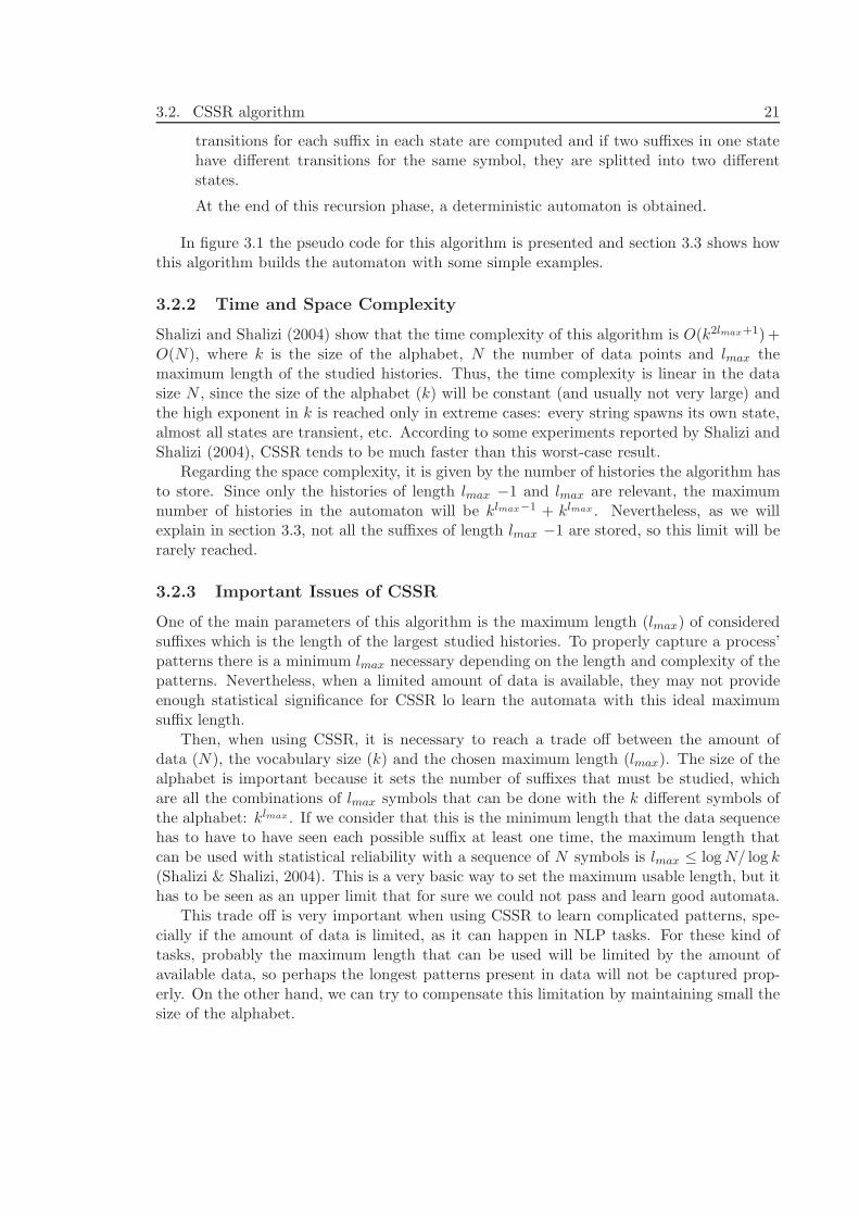
3.2. CSSR algorithm 21
transitions for each suffix in each state are computed and if two suffixes in one statehave different transitions for the same symbol, they are splitted into two differentstates.
At the end of this recursion phase, a deterministic automaton is obtained.
In figure 3.1 the pseudo code for this algorithm is presented and section 3.3 shows howthis algorithm builds the automaton with some simple examples.
3.2.2 Time and Space Complexity
Shalizi and Shalizi (2004) show that the time complexity of this algorithm is O(k2lmax+1)+O(N), where k is the size of the alphabet, N the number of data points and lmax themaximum length of the studied histories. Thus, the time complexity is linear in the datasize N , since the size of the alphabet (k) will be constant (and usually not very large) andthe high exponent in k is reached only in extreme cases: every string spawns its own state,almost all states are transient, etc. According to some experiments reported by Shalizi andShalizi (2004), CSSR tends to be much faster than this worst-case result.
Regarding the space complexity, it is given by the number of histories the algorithm hasto store. Since only the histories of length lmax −1 and lmax are relevant, the maximumnumber of histories in the automaton will be klmax−1 + klmax . Nevertheless, as we willexplain in section 3.3, not all the suffixes of length lmax −1 are stored, so this limit will berarely reached.
3.2.3 Important Issues of CSSR
One of the main parameters of this algorithm is the maximum length (lmax) of consideredsuffixes which is the length of the largest studied histories. To properly capture a process’patterns there is a minimum lmax necessary depending on the length and complexity of thepatterns. Nevertheless, when a limited amount of data is available, they may not provideenough statistical significance for CSSR lo learn the automata with this ideal maximumsuffix length.
Then, when using CSSR, it is necessary to reach a trade off between the amount ofdata (N), the vocabulary size (k) and the chosen maximum length (lmax). The size of thealphabet is important because it sets the number of suffixes that must be studied, whichare all the combinations of lmax symbols that can be done with the k different symbols ofthe alphabet: klmax . If we consider that this is the minimum length that the data sequencehas to have to have seen each possible suffix at least one time, the maximum length thatcan be used with statistical reliability with a sequence of N symbols is lmax ≤ log N/ log k(Shalizi & Shalizi, 2004). This is a very basic way to set the maximum usable length, but ithas to be seen as an upper limit that for sure we could not pass and learn good automata.
This trade off is very important when using CSSR to learn complicated patterns, spe-cially if the amount of data is limited, as it can happen in NLP tasks. For these kind oftasks, probably the maximum length that can be used will be limited by the amount ofavailable data, so perhaps the longest patterns present in data will not be captured prop-erly. On the other hand, we can try to compensate this limitation by maintaining small thesize of the alphabet.
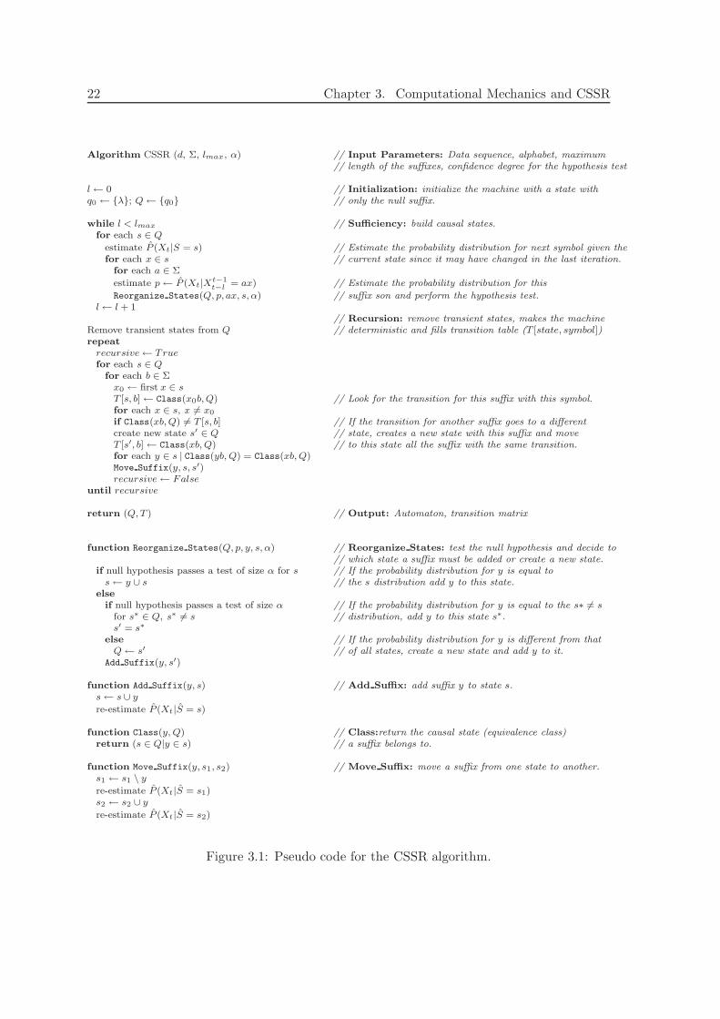
22 Chapter 3. Computational Mechanics and CSSR
Algorithm CSSR (d, Σ, lmax, α) // Input Parameters: Data sequence, alphabet, maximum// length of the suffixes, confidence degree for the hypothesis test
l← 0 // Initialization: initialize the machine with a state withq0 ← {λ}; Q← {q0} // only the null suffix.
while l < lmax // Sufficiency: build causal states.for each s ∈ Q
estimate P (Xt|S = s) // Estimate the probability distribution for next symbol given thefor each x ∈ s // current state since it may have changed in the last iteration.
for each a ∈ Σ
estimate p← P (Xt|Xt−1
t−l= ax) // Estimate the probability distribution for this
Reorganize States(Q, p, ax, s, α) // suffix son and perform the hypothesis test.l← l + 1
// Recursion: remove transient states, makes the machineRemove transient states from Q // deterministic and fills transition table (T [state, symbol])repeat
recursive← True
for each s ∈ Q
for each b ∈ Σx0 ← first x ∈ s
T [s, b]← Class(x0b, Q) // Look for the transition for this suffix with this symbol.for each x ∈ s, x 6= x0
if Class(xb, Q) 6= T [s, b] // If the transition for another suffix goes to a differentcreate new state s′ ∈ Q // state, creates a new state with this suffix and moveT [s′, b]← Class(xb, Q) // to this state all the suffix with the same transition.for each y ∈ s | Class(yb, Q) = Class(xb, Q)Move Suffix(y, s, s′)recursive← False
until recursive
return (Q, T ) // Output: Automaton, transition matrix
function Reorganize States(Q, p, y, s, α) // Reorganize States: test the null hypothesis and decide to// which state a suffix must be added or create a new state.
if null hypothesis passes a test of size α for s // If the probability distribution for y is equal tos← y ∪ s // the s distribution add y to this state.
else
if null hypothesis passes a test of size α // If the probability distribution for y is equal to the s∗ 6= s
for s∗ ∈ Q, s∗ 6= s // distribution, add y to this state s∗.s′ = s∗
else // If the probability distribution for y is different from thatQ← s′ // of all states, create a new state and add y to it.
Add Suffix(y, s′)
function Add Suffix(y, s) // Add Suffix: add suffix y to state s.s← s ∪ y
re-estimate P (Xt|S = s)
function Class(y, Q) // Class:return the causal state (equivalence class)return (s ∈ Q|y ∈ s) // a suffix belongs to.
function Move Suffix(y, s1, s2) // Move Suffix: move a suffix from one state to another.s1 ← s1 \ y
re-estimate P (Xt|S = s1)s2 ← s2 ∪ y
re-estimate P (Xt|S = s2)
Figure 3.1: Pseudo code for the CSSR algorithm.
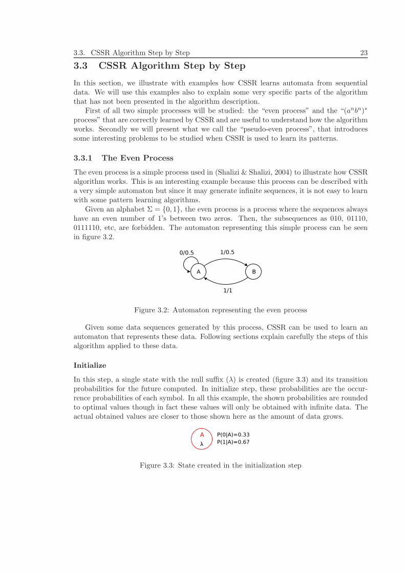
3.3. CSSR Algorithm Step by Step 23
3.3 CSSR Algorithm Step by Step
In this section, we illustrate with examples how CSSR learns automata from sequentialdata. We will use this examples also to explain some very specific parts of the algorithmthat has not been presented in the algorithm description.
First of all two simple processes will be studied: the “even process” and the “(anbn)∗
process” that are correctly learned by CSSR and are useful to understand how the algorithmworks. Secondly we will present what we call the “pseudo-even process”, that introducessome interesting problems to be studied when CSSR is used to learn its patterns.
3.3.1 The Even Process
The even process is a simple process used in (Shalizi & Shalizi, 2004) to illustrate how CSSRalgorithm works. This is an interesting example because this process can be described witha very simple automaton but since it may generate infinite sequences, it is not easy to learnwith some pattern learning algorithms.
Given an alphabet Σ = {0, 1}, the even process is a process where the sequences alwayshave an even number of 1’s between two zeros. Then, the subsequences as 010, 01110,0111110, etc, are forbidden. The automaton representing this simple process can be seenin figure 3.2.
Figure 3.2: Automaton representing the even process
Given some data sequences generated by this process, CSSR can be used to learn anautomaton that represents these data. Following sections explain carefully the steps of thisalgorithm applied to these data.
Initialize
In this step, a single state with the null suffix (λ) is created (figure 3.3) and its transitionprobabilities for the future computed. In initialize step, these probabilities are the occur-rence probabilities of each symbol. In all this example, the shown probabilities are roundedto optimal values though in fact these values will only be obtained with infinite data. Theactual obtained values are closer to those shown here as the amount of data grows.
Figure 3.3: State created in the initialization step
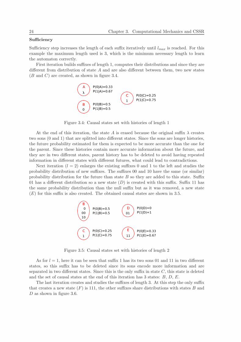
24 Chapter 3. Computational Mechanics and CSSR
Sufficiency
Sufficiency step increases the length of each suffix iteratively until lmax is reached. For thisexample the maximum length used is 3, which is the minimum necessary length to learnthe automaton correctly.
First iteration builds suffixes of length 1, computes their distributions and since they aredifferent from distribution of state A and are also different between them, two new states(B and C) are created, as shown in figure 3.4.
Figure 3.4: Causal states set with histories of length 1
At the end of this iteration, the state A is erased because the original suffix λ createstwo sons (0 and 1) that are splitted into different states. Since the sons are longer histories,the future probability estimated for them is expected to be more accurate than the one forthe parent. Since these histories contain more accurate information about the future, andthey are in two different states, parent history has to be deleted to avoid having repeatedinformation in different states with different futures, what could lead to contradictions.
Next iteration (l = 2) enlarges the existing suffixes 0 and 1 to the left and studies theprobability distribution of new suffixes. The suffixes 00 and 10 have the same (or similar)probability distribution for the future than state B so they are added to this state. Suffix01 has a different distribution so a new state (D) is created with this suffix. Suffix 11 hasthe same probability distribution than the null suffix but as it was removed, a new state(E) for this suffix is also created. The obtained causal states are shown in 3.5.
Figure 3.5: Causal states set with histories of length 2
As for l = 1, here it can be seen that suffix 1 has its two sons 01 and 11 in two differentstates, so this suffix has to be deleted since its sons encode more information and areseparated in two different states. Since this is the only suffix in state C, this state is deletedand the set of causal states at the end of this iteration has 3 states: B, D, E.
The last iteration creates and studies the suffixes of length 3. At this step the only suffixthat creates a new state (F ) is 111, the other suffixes share distributions with states B andD as shown in figure 3.6.
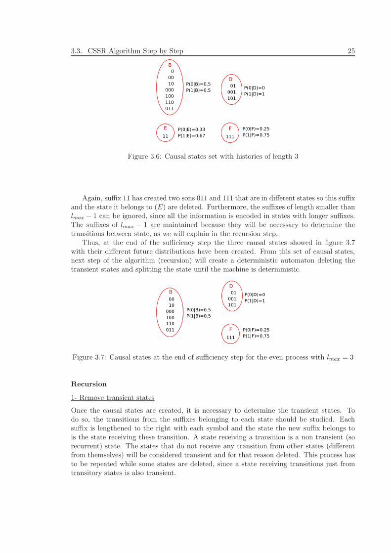
3.3. CSSR Algorithm Step by Step 25
Figure 3.6: Causal states set with histories of length 3
Again, suffix 11 has created two sons 011 and 111 that are in different states so this suffixand the state it belongs to (E) are deleted. Furthermore, the suffixes of length smaller thanlmax − 1 can be ignored, since all the information is encoded in states with longer suffixes.The suffixes of lmax − 1 are maintained because they will be necessary to determine thetransitions between state, as we will explain in the recursion step.
Thus, at the end of the sufficiency step the three causal states showed in figure 3.7with their different future distributions have been created. From this set of causal states,next step of the algorithm (recursion) will create a deterministic automaton deleting thetransient states and splitting the state until the machine is deterministic.
Figure 3.7: Causal states at the end of sufficiency step for the even process with lmax = 3
Recursion
1- Remove transient states
Once the causal states are created, it is necessary to determine the transient states. Todo so, the transitions from the suffixes belonging to each state should be studied. Eachsuffix is lengthened to the right with each symbol and the state the new suffix belongs tois the state receiving these transition. A state receiving a transition is a non transient (sorecurrent) state. The states that do not receive any transition from other states (differentfrom themselves) will be considered transient and for that reason deleted. This process hasto be repeated while some states are deleted, since a state receiving transitions just fromtransitory states is also transient.
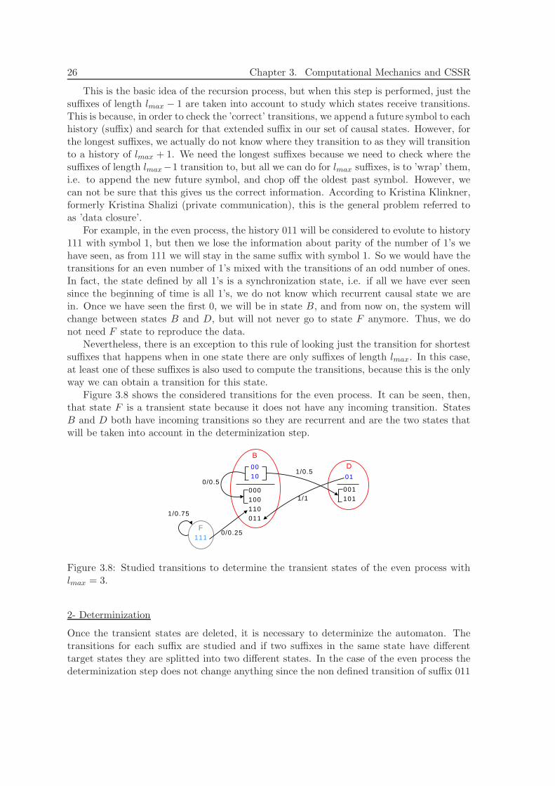
26 Chapter 3. Computational Mechanics and CSSR
This is the basic idea of the recursion process, but when this step is performed, just thesuffixes of length lmax − 1 are taken into account to study which states receive transitions.This is because, in order to check the ’correct’ transitions, we append a future symbol to eachhistory (suffix) and search for that extended suffix in our set of causal states. However, forthe longest suffixes, we actually do not know where they transition to as they will transitionto a history of lmax + 1. We need the longest suffixes because we need to check where thesuffixes of length lmax−1 transition to, but all we can do for lmax suffixes, is to ’wrap’ them,i.e. to append the new future symbol, and chop off the oldest past symbol. However, wecan not be sure that this gives us the correct information. According to Kristina Klinkner,formerly Kristina Shalizi (private communication), this is the general problem referred toas ’data closure’.
For example, in the even process, the history 011 will be considered to evolute to history111 with symbol 1, but then we lose the information about parity of the number of 1’s wehave seen, as from 111 we will stay in the same suffix with symbol 1. So we would have thetransitions for an even number of 1’s mixed with the transitions of an odd number of ones.In fact, the state defined by all 1’s is a synchronization state, i.e. if all we have ever seensince the beginning of time is all 1’s, we do not know which recurrent causal state we arein. Once we have seen the first 0, we will be in state B, and from now on, the system willchange between states B and D, but will not never go to state F anymore. Thus, we donot need F state to reproduce the data.
Nevertheless, there is an exception to this rule of looking just the transition for shortestsuffixes that happens when in one state there are only suffixes of length lmax. In this case,at least one of these suffixes is also used to compute the transitions, because this is the onlyway we can obtain a transition for this state.
Figure 3.8 shows the considered transitions for the even process. It can be seen, then,that state F is a transient state because it does not have any incoming transition. StatesB and D both have incoming transitions so they are recurrent and are the two states thatwill be taken into account in the determinization step.
D01
001101
B
000100110011
0010
0/0.5
F111
1/0.5
1/1
0/0.25
1/0.75
Figure 3.8: Studied transitions to determine the transient states of the even process withlmax = 3.
2- Determinization
Once the transient states are deleted, it is necessary to determinize the automaton. Thetransitions for each suffix are studied and if two suffixes in the same state have differenttarget states they are splitted into two different states. In the case of the even process thedeterminization step does not change anything since the non defined transition of suffix 011
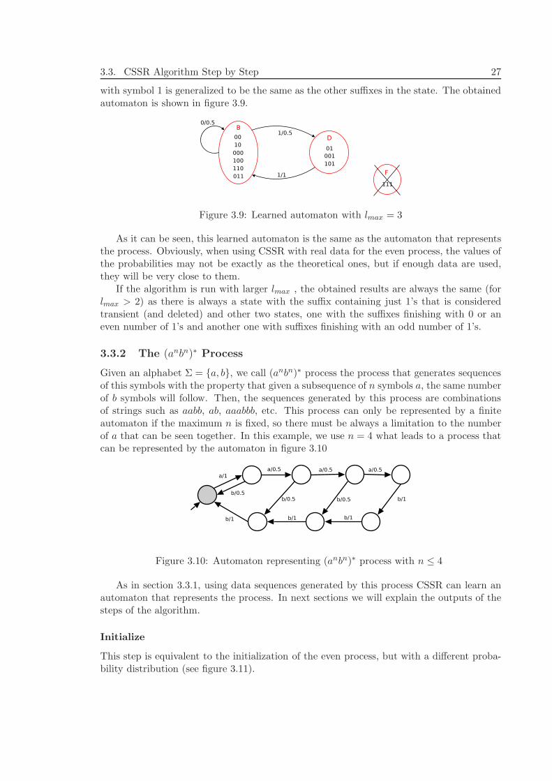
3.3. CSSR Algorithm Step by Step 27
with symbol 1 is generalized to be the same as the other suffixes in the state. The obtainedautomaton is shown in figure 3.9.
Figure 3.9: Learned automaton with lmax = 3
As it can be seen, this learned automaton is the same as the automaton that representsthe process. Obviously, when using CSSR with real data for the even process, the values ofthe probabilities may not be exactly as the theoretical ones, but if enough data are used,they will be very close to them.
If the algorithm is run with larger lmax , the obtained results are always the same (forlmax > 2) as there is always a state with the suffix containing just 1’s that is consideredtransient (and deleted) and other two states, one with the suffixes finishing with 0 or aneven number of 1’s and another one with suffixes finishing with an odd number of 1’s.
3.3.2 The (anbn)∗ Process
Given an alphabet Σ = {a, b}, we call (anbn)∗ process the process that generates sequencesof this symbols with the property that given a subsequence of n symbols a, the same numberof b symbols will follow. Then, the sequences generated by this process are combinationsof strings such as aabb, ab, aaabbb, etc. This process can only be represented by a finiteautomaton if the maximum n is fixed, so there must be always a limitation to the numberof a that can be seen together. In this example, we use n = 4 what leads to a process thatcan be represented by the automaton in figure 3.10
Figure 3.10: Automaton representing (anbn)∗ process with n ≤ 4
As in section 3.3.1, using data sequences generated by this process CSSR can learn anautomaton that represents the process. In next sections we will explain the outputs of thesteps of the algorithm.
Initialize
This step is equivalent to the initialization of the even process, but with a different proba-bility distribution (see figure 3.11).
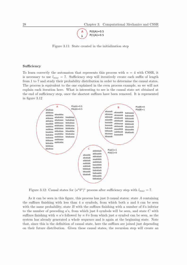
28 Chapter 3. Computational Mechanics and CSSR
Figure 3.11: State created in the initialization step
Sufficiency
To learn correctly the automaton that represents this process with n = 4 with CSSR, itis necessary to use lmax = 7. Sufficiency step will iteratively create each suffix of lengthfrom 1 to 7 and study their probability distribution in order to determine the causal states.The process is equivalent to the one explained in the even process example, so we will notexplain each iteration here. What is interesting to see is the causal state set obtained atthe end of sufficiency step, once the shortest suffixes have been removed. It is representedin figure 3.12
Figure 3.12: Causal states for (anbn)∗ process after sufficiency step with lmax = 7.
As it can be seen in this figure, this process has just 3 causal states: state A containingthe suffixes finishing with less than 4 a symbols, from which both a and b can be seenwith the same probability, state B with the suffixes finishing with a number of b’s inferiorto the number of preceding a’s, from which just b symbols will be seen, and state C withsuffixes finishing with n a’s followed by n b’s from which just a symbol can be seen, as thesystem has already generated a whole sequence and is again at the beginning state. Notethat, since this is the definition of causal state, here the suffixes are joined just dependingon their future distribution. Given these causal states, the recursion step will create an
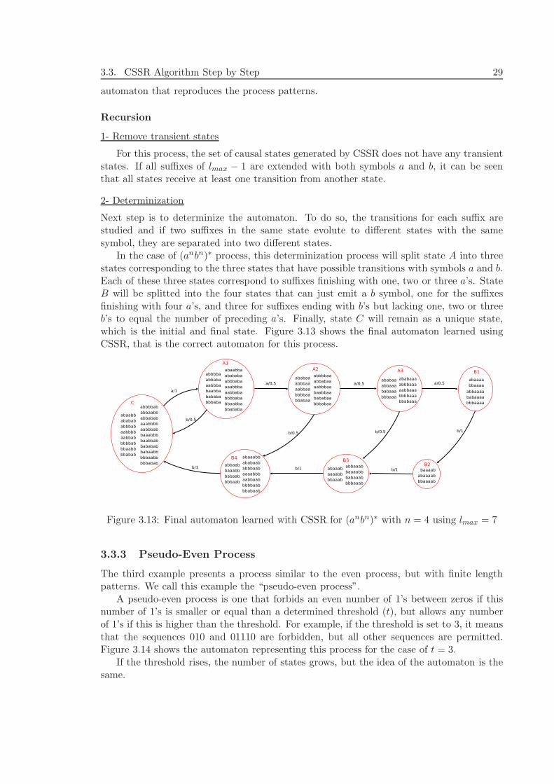
3.3. CSSR Algorithm Step by Step 29
automaton that reproduces the process patterns.
Recursion
1- Remove transient states
For this process, the set of causal states generated by CSSR does not have any transientstates. If all suffixes of lmax − 1 are extended with both symbols a and b, it can be seenthat all states receive at least one transition from another state.
2- Determinization
Next step is to determinize the automaton. To do so, the transitions for each suffix arestudied and if two suffixes in the same state evolute to different states with the samesymbol, they are separated into two different states.
In the case of (anbn)∗ process, this determinization process will split state A into threestates corresponding to the three states that have possible transitions with symbols a and b.Each of these three states correspond to suffixes finishing with one, two or three a’s. StateB will be splitted into the four states that can just emit a b symbol, one for the suffixesfinishing with four a’s, and three for suffixes ending with b’s but lacking one, two or threeb’s to equal the number of preceding a’s. Finally, state C will remain as a unique state,which is the initial and final state. Figure 3.13 shows the final automaton learned usingCSSR, that is the correct automaton for this process.
Figure 3.13: Final automaton learned with CSSR for (anbn)∗ with n = 4 using lmax = 7
3.3.3 Pseudo-Even Process
The third example presents a process similar to the even process, but with finite lengthpatterns. We call this example the “pseudo-even process”.
A pseudo-even process is one that forbids an even number of 1’s between zeros if thisnumber of 1’s is smaller or equal than a determined threshold (t), but allows any numberof 1’s if this is higher than the threshold. For example, if the threshold is set to 3, it meansthat the sequences 010 and 01110 are forbidden, but all other sequences are permitted.Figure 3.14 shows the automaton representing this process for the case of t = 3.
If the threshold rises, the number of states grows, but the idea of the automaton is thesame.
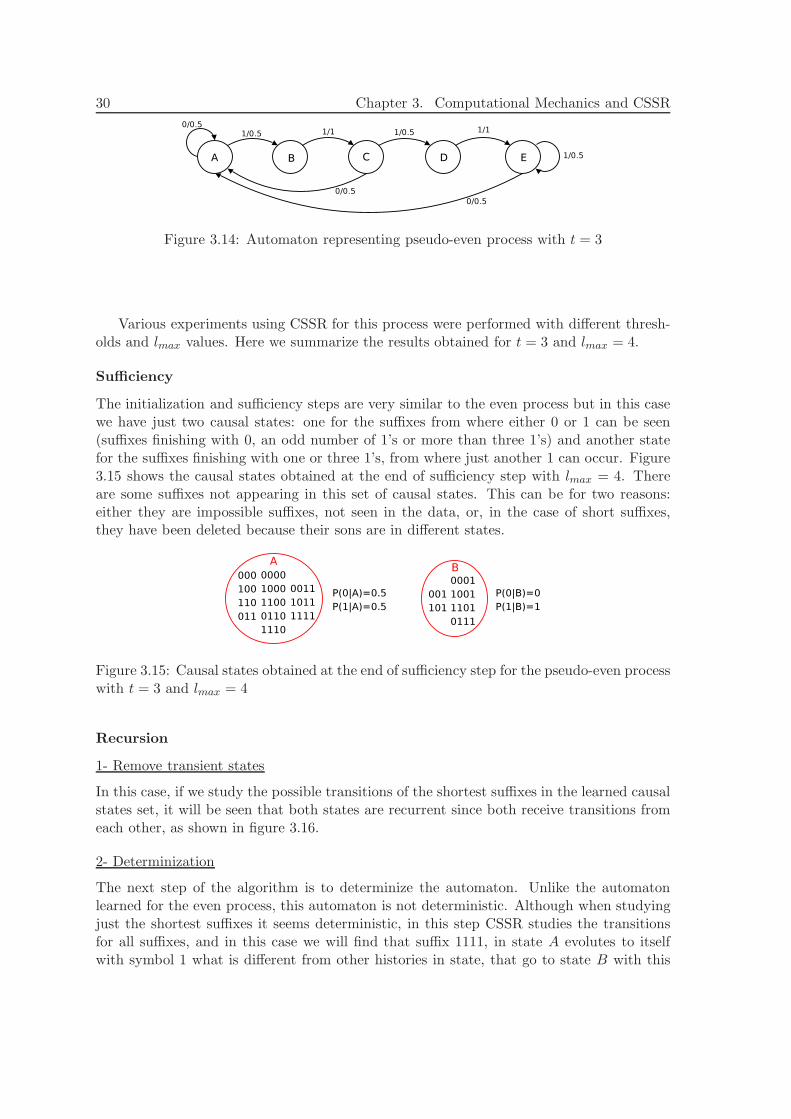
30 Chapter 3. Computational Mechanics and CSSR
Figure 3.14: Automaton representing pseudo-even process with t = 3
Various experiments using CSSR for this process were performed with different thresh-olds and lmax values. Here we summarize the results obtained for t = 3 and lmax = 4.
Sufficiency
The initialization and sufficiency steps are very similar to the even process but in this casewe have just two causal states: one for the suffixes from where either 0 or 1 can be seen(suffixes finishing with 0, an odd number of 1’s or more than three 1’s) and another statefor the suffixes finishing with one or three 1’s, from where just another 1 can occur. Figure3.15 shows the causal states obtained at the end of sufficiency step with lmax = 4. Thereare some suffixes not appearing in this set of causal states. This can be for two reasons:either they are impossible suffixes, not seen in the data, or, in the case of short suffixes,they have been deleted because their sons are in different states.
Figure 3.15: Causal states obtained at the end of sufficiency step for the pseudo-even processwith t = 3 and lmax = 4
Recursion
1- Remove transient states
In this case, if we study the possible transitions of the shortest suffixes in the learned causalstates set, it will be seen that both states are recurrent since both receive transitions fromeach other, as shown in figure 3.16.
2- Determinization
The next step of the algorithm is to determinize the automaton. Unlike the automatonlearned for the even process, this automaton is not deterministic. Although when studyingjust the shortest suffixes it seems deterministic, in this step CSSR studies the transitionsfor all suffixes, and in this case we will find that suffix 1111, in state A evolutes to itselfwith symbol 1 what is different from other histories in state, that go to state B with this
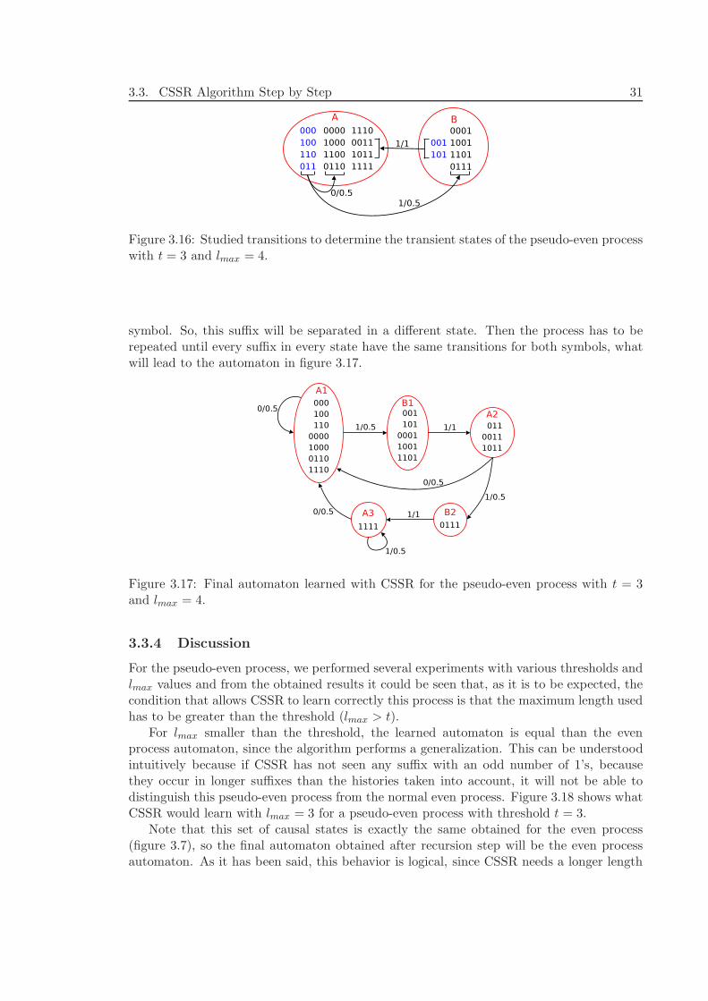
3.3. CSSR Algorithm Step by Step 31
Figure 3.16: Studied transitions to determine the transient states of the pseudo-even processwith t = 3 and lmax = 4.
symbol. So, this suffix will be separated in a different state. Then the process has to berepeated until every suffix in every state have the same transitions for both symbols, whatwill lead to the automaton in figure 3.17.
Figure 3.17: Final automaton learned with CSSR for the pseudo-even process with t = 3and lmax = 4.
3.3.4 Discussion
For the pseudo-even process, we performed several experiments with various thresholds andlmax values and from the obtained results it could be seen that, as it is to be expected, thecondition that allows CSSR to learn correctly this process is that the maximum length usedhas to be greater than the threshold (lmax > t).
For lmax smaller than the threshold, the learned automaton is equal than the evenprocess automaton, since the algorithm performs a generalization. This can be understoodintuitively because if CSSR has not seen any suffix with an odd number of 1’s, becausethey occur in longer suffixes than the histories taken into account, it will not be able todistinguish this pseudo-even process from the normal even process. Figure 3.18 shows whatCSSR would learn with lmax = 3 for a pseudo-even process with threshold t = 3.
Note that this set of causal states is exactly the same obtained for the even process(figure 3.7), so the final automaton obtained after recursion step will be the even processautomaton. As it has been said, this behavior is logical, since CSSR needs a longer length
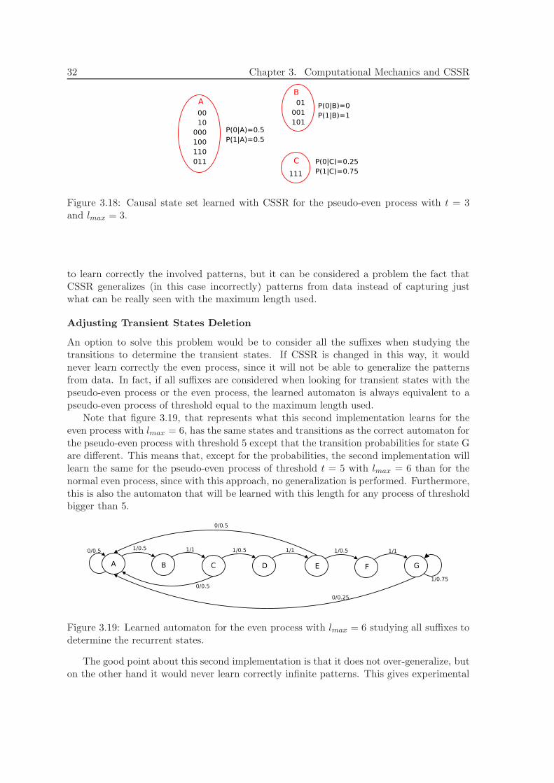
32 Chapter 3. Computational Mechanics and CSSR
Figure 3.18: Causal state set learned with CSSR for the pseudo-even process with t = 3and lmax = 3.
to learn correctly the involved patterns, but it can be considered a problem the fact thatCSSR generalizes (in this case incorrectly) patterns from data instead of capturing justwhat can be really seen with the maximum length used.
Adjusting Transient States Deletion
An option to solve this problem would be to consider all the suffixes when studying thetransitions to determine the transient states. If CSSR is changed in this way, it wouldnever learn correctly the even process, since it will not be able to generalize the patternsfrom data. In fact, if all suffixes are considered when looking for transient states with thepseudo-even process or the even process, the learned automaton is always equivalent to apseudo-even process of threshold equal to the maximum length used.
Note that figure 3.19, that represents what this second implementation learns for theeven process with lmax = 6, has the same states and transitions as the correct automaton forthe pseudo-even process with threshold 5 except that the transition probabilities for state Gare different. This means that, except for the probabilities, the second implementation willlearn the same for the pseudo-even process of threshold t = 5 with lmax = 6 than for thenormal even process, since with this approach, no generalization is performed. Furthermore,this is also the automaton that will be learned with this length for any process of thresholdbigger than 5.
Figure 3.19: Learned automaton for the even process with lmax = 6 studying all suffixes todetermine the recurrent states.
The good point about this second implementation is that it does not over-generalize, buton the other hand it would never learn correctly infinite patterns. This gives experimental
3.4. CSSR compared with other techniques 33
evidence that the fact of using just the short suffixes to determine the recurrent states isthe correct option, as it has been argued in section 3.3.1, specially if we want to use allpower of causal states. Nevertheless, this example also shows that if lmax is too small forthe involved patterns, the learned automaton will not be correct, since it will not either becorrect using the alternative implementation. This must be taken into account for furtherexperiments in NLP tasks. Let’s take for example the chunking task, where CSSR will notbe able to capture chunk structure of length l using lmax < l. Furthermore, given that thelimited amount of data will limit the maximum possible value of lmax to be used, we haveto take into account that longest chunk patterns would be probably lost.
Nevertheless, we can expect that as CSSR is able to perform generalization from data,it will be able to learn patterns that are not specifically present in the data but are alsopossible in natural language sequences. On the other hand, though, it can also be arguedthat for NLP patterns it will be better that CSSR does not generalize anything (taking intoaccount all suffixes when determining recurrent states), since we can prefer the system notto generalize from data but to learn just the patterns that has been seen with the lmax used.In this thesis, we will study the influence of these two possible approaches when applied toNLP tasks.
3.4 CSSR compared with other techniques
In this section, we discuss the difference between CSSR algorithm (and ǫ-machines in gen-eral) and the algorithms presented in chapter 2 that are closer to this technique: MarkovModels, VLMM and Suffix Trees. We will also compare CSSR with other algorithms thatlearn ǫ-machines.
3.4.1 ǫ-machines versus Markov Models
Once causal states have been reduced to sets of suffixes of a maximum determined length,ǫ-machines have the form of Markov Models (MM), where a state is build for each possiblen-gram (equivalent to a suffix).
Then, the many desirable features of MMs are secured for ǫ-machine, but the laterintroduce some interesting features that Markov Models lack. One of the main new is-sues of ǫ-machines with respect to Markov Models is that for ǫ-machines it is not ne-cessary to make any a priory assumptions about the architecture of the system. Eachǫ-machine reconstruction algorithm builds an automaton grouping the histories dependingon their future distribution probabilities while MM create a state for each possible suffix.Furthermore, since causal states join various histories in each state, the size of the gene-rated automaton will be really smaller than the equivalent MM. This could be very usefulin systems where the amount of data limits the order of the MM that can be learned. Wecan expect to be able to learn an equivalent ǫ-machine with longer histories with the samememory. Of course, it depends on the studied process how many suffixes will be groupedinto a causal states, and thus, how much bigger will be the Markov Model with respect tothe ǫ-machine.
Another issue to take into account is that in terms of Markov Models, lmax −1 would bethe potential maximum order of the model. If the generated ǫ-machine would have a statefor each history we would get a Markov Model of order lmax − 1.
34 Chapter 3. Computational Mechanics and CSSR
3.4.2 ǫ-machines versus VLMM and Prediction Suffix Trees
Variable Memory Length Markov Models (Rissanen, 1983; Buhlmann & Wyner, 1999;Willems et al., 1995; Tino & Dorner, 2001) and Prediction Suffix Trees (Ron et al., 1994b;Ron et al., 1994a) properties can be studied together since from one given description ofdata with one of this two techniques, it is always possible to create an equivalent descriptionwith the other. In this section, we will compare both to ǫ-machines.
With all ǫ-machines, PST and VLMM, states may be regarded as classes of histories ofthe observable process. With a PST or a VLMM, every state is defined by a single suffix, andconsists of all and only the histories ending in that suffix. The crucial distinction is that thestates in an ǫ-machine are not defined by unique suffixes, but may contain multiple suffixesrepresenting different contexts that can lead to that state. Furthermore, there are processeswith a finite causal-state representation which do not have finite suffix-tree representations.An example of such a process is the “even process” (see section 3.3.1) that needs an infinitePST to be represented correctly.
The strength of ǫ-machines is that by joining some suffixes in the same state, theyperform a generalization capable of building automata for reproducing infinite process. Thiscan not be done using VLMM or PST. On the other hand, every process with a finite suffixtree representation has a finite causal state model, which is discoverable by CSSR or someother ǫ-machine reconstruction algorithm. Thus, CSSR can be considered more powerfulthan learning PST and for that reason we are interested in studying its performance in NLPtasks.
On the other hand, VLMM and PST have the advantage over CSSR that while CSSRstudies all histories up to a fixed maximum length, VLMM and PST consider just longsuffixes when necessary, leaving some suffixes unexplored when they do not seem to intro-duce different statistical information. In this way, it can be claimed that VLMM and PSTcan deal with longer maximum lengths, since they do not need to study all suffixes, but asCSSR groups histories in states, the computational need is always reduced with respect tothe needs of an HMM for example, so CSSR can still compete with VLMM and PST in thisaspect.
ǫ-machines, VLMM and PSTs have the advantage over HMMs that the architectureof the system is learned according to the data rather than being predefined as in HMMs.Thus, the number of generated states with these methods is expected to be less than |Σ|L
(where |Σ| is the size of the alphabet, this is, the number of considered symbols and L isthe maximum length of the considered suffixes), which would be the number of states ina HMM.
3.4.3 CSSR versus other ǫ-machine learning algorithms.
The main difference between CSSR and State-Merging ǫ-Machine Inference algorithms(Crutchfield & Young, 1989; Crutchfield & Young, 1990; Hanson, 1993; Crutchfield, 1994)is that while CSSR starts considering that all the suffixes belong to the same state andconstructs the automaton splitting the states when necessary, State-Merging ǫ-Machine In-ference algorithms start assuming that each suffix belongs to a state and is whittled downby merging.
As algorithms that infere ǫ-machines, CSSR and State-Merging ǫ-Machine Inferencealgorithms both have the same domain of applicability, but CSSR is more well-behaved andconverges faster than merging methods.
3.5. CSSR applications 35
Furthermore, CSSR makes use of some properties about causal states (they are determi-nistic, Markovian, etc) to guide the search, the automaton construction. This informationis not used by other reconstruction algorithms.
3.5 CSSR applications
CSSR has been applied to various research areas. Here we present a review of these appli-cations and the obtained results.
Varn and Crutchfield (2004) analyze solid-state phase transformations. They study thetransition of annealed ZnS crystals between two different solid structures: 2H and 3C. ZnScrystals are stable in one of these two phases depending on the temperature. These twophases can be characterized by the inter-ML spin distribution. This is, the patterns of spinvalues of consecutive atoms.
In that work, they study the spatial configuration of the crystals in terms of the spinposition during the transformation, given a parameter f that models how close is the crystalto one of the two phases. When f=0 the system is in 2H phase, and for f=1 in 3C. Thespin position depending on f and on the position in the crystal form the data that CSSRuses to construct an ǫ-machine. This machine models the structural description of thespin configuration in various steps of the transformation (i.e. various f values). Thus, thelearned automaton reproduces the observed spin sequences in the different stages of thetransformation. The alphabet used in the transitions has only the two possible spin valuesvalues, 0 and 1. The parameter f modifies the transition probabilities modeling in this waythe two possible phases and the transition stages. Then, the built automaton changes theallowed transitions depending on f modelling the two different phases and the intermediatestages.
In this framework, CSSR is used to obtain a readable automaton that models the pat-terns of the two phase crystals and also modelling the transition between them. With thissmall alphabet and a relatively simple structure two be detected the algorithm is useful andbuilds accurate automata.
Another CSSR application is presented by Ray (2004). The goal of this work is to per-form anomaly detection in complex dynamical systems using tools as Symbolic Dynamics,Finite State Automata and Pattern Recognition.
In a dynamical system, an anomaly is a deviation from its nominal behavior. The ideaof the presented work is to use pattern acquisition techniques to build a patterns of thenormal behavior of a system and then use this pattern to detect deviations in new data. Todo so it is necessary to define a measure of the deviation from the pattern to determine if anobservation can be considered an anomaly or not. They also try to deduce if the anomalyhas any pattern.
In fact, Ray (2004) uses CSSR theoretical work to develop a pattern representation,named D-markov chains that is simpler than ǫ-machines and capture enough informationfor anomaly detection.
One application in the field of Sociology and also related to Natural Language Processingis presented in (Cointet et al., 2007). The aim of this work is to investigate how variousinformation sources such as weblogs and on-line media are intertemporaly correlated.
To do so, they study the presence of 75 relevant topics in 33 French political corpus and6 on-line press sources during 30 days. Three categories are built with the blogs depending
36 Chapter 3. Computational Mechanics and CSSR
on its similarity and a fourth category is used for press. Then, they want to model theinteraction between these 4 categories using CSSR algorithm.
The alphabet is created in the following way: for each term, consider the frequencyof appearing in each category. If this frequency (properly normalized) is bigger than adetermined threshold, the term is considered to appear in this category. Then, each symbolof the alphabet is a possible appearing combination of a term or not appearing in eachcategory. So the alphabet has 24 = 16 symbols.
Thus the presence of each term in the various categories for the different days can beencoded as a sequence of alphabet symbols, one symbol for each day. Using the differentterms they expect to find more correlations, since it increases the number of instances.
Using the data encoded in this way, they use CSSR to learn an automaton represent-ing the causal structure of the data. They interpret the possible transitions as existingcorrelations between groups of blogs having also the probabilities of this correlations.
All the systems presented so far use CSSR as a way to capture the patterns of somedata in order to try to understand the behavior of a determined process. Another use ofCSSR found in the literature is to use the algorithm to study the complexity of a systemor of a data set.
In this line, Shalizi (2001) and Shalizi et al. (2004) propose the use of computationalmechanics and CSSR to compute the statistical complexity of a process as defined byCrutchfield and Young (1989). Via the use of the algorithm, not only the statistical com-plexity of the process can be measured, but also a proposal to define ”emergence” and”self-organization” in complex systems is presented. The ideas can be applied to bothtemporal and spatial patterns.
Following the same line, Boschetti (2007) defines the complexity of an ecological model asthe statistical complexity of the output it produces. It is important to define this complexitymeasure because the ecological models, to become more accurate, are growing in complexity(taking into account more parameters, processes, etc.). This makes the models less tractable,so it is necessary to reach a trade off between the accuracy of the model and its complexity.To do so, it is necessary not only to define but also to measure the complexity of ecologicalmodels. The proposal of Boschetti (2007) is to use CSSR to measure this complexity,similarly to the work presented in (Shalizi, 2001; Shalizi et al., 2004).
Also, Park et al. (2006) present an approach to use CSSR to compute the complexity andentropy density of the Korean stock market. The idea is to use CSSR to learn an automatonthat models the variation on the Korean Composition Stock Price Index (KOSPI) alongtime. The time series formed by the variation of this index is converted into a binary timeseries depending on whether the variation is positive or negative. With these data, anǫ-machine is computed using CSSR for each year and the complexity of the time series iscomputed and compared along the different years. Furthermore, the machine is also usedto compute the entropy density, that shows how random the process is.
In this thesis, first of all we will study the CSSR ability to learn patterns related to NLPdata, since it has been seen that the algorithm is useful to capture patterns in other researchfields. Nevertheless, the main goal of this thesis is to apply CSSR to NLP annotation tasks.To do so, it is necessary to introduce some hidden information into the system in order thatit can learn an automaton that can be afterwards used to annotate new sentences. As faras we know, there is no previous work in NLP or other fields in the line of using CSSR forannotation tasks.

CHAPTER 4
Study of CSSR Ability to Capture Language
Subsequence Patterns
Before applying CSSR algorithm to annotation NLP tasks, some experiments to studythe ability of CSSR to capture the patterns that form some language subsequences wereperformed. The goal of these experiments is to prove that this method is able to capturesentence patterns, as well as to study the influence of the various parameters.
This chapter presents these experiments, that conform a study of the applicability ofCSSR to some NLP basic tasks. For this first study, no annotation tasks are performedsince we are just interested on studying the patterns that CSSR can learn in the NLP fieldto see if it can be useful for the annotation tasks.
The experiments are focused on studying the patterns of Named Entities (NEs) andNoun Phrase (NP) chunks that CSSR learns. It will be seen that the algorithm is able tocapture the patterns of these language subsequences, and the conditions under which thealgorithm performs better and the limitations of CSSR will be discussed.
For NE patterns, we will show that CSSR is able to learn intuitive automata that capturethe patterns of sentences in terms of the selected alphabet. For NP patterns, we will seethat the learned automata are not so easily interpretable, since they are bigger, so wewill propose another way to qualitatively evaluate the correctness of the CSSR automata.Furthermore, and to study the influence of the available amount of data, we will presentsome experiments with artificially generated data and we will see how the learned automatareproduce better the NP patterns when more data is available.
The study of the patterns learned for NEs, presented in section 4.2, was published in(Padro & Padro, 2005c) and the study for NPs (section 4.3) can be found in (Padro &Padro, 2007b).
37
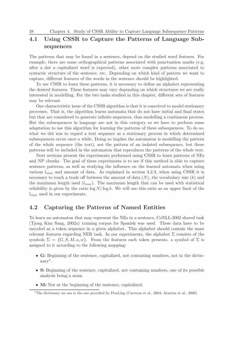
38 Chapter 4. Study of CSSR Ability to Capture Language Subsequence Patterns
4.1 Using CSSR to Capture the Patterns of Language Sub-
sequences
The patterns that may be found in a sentence, depend on the studied word features. Forexample, there are some orthographical patterns associated with punctuation marks (e.g.after a dot a capitalized word is expected), other more complex patterns associated tosyntactic structure of the sentence, etc. Depending on which kind of pattern we want tocapture, different features of the words in the sentence should be highlighted.
To use CSSR to learn these patterns, it is necessary to define an alphabet representingthe desired features. These features may vary depending on which structures we are reallyinterested in modelling. For the two tasks studied in this chapter, different sets of featuresmay be relevant.
One characteristic issue of the CSSR algorithm is that it is conceived to model stationaryprocesses. That is, the algorithm learns automata that do not have initial and final statesbut that are considered to generate infinite sequences, thus modelling a continuous process.But the subsequences in language are not in this category so we have to perform someadaptation to use this algorithm for learning the patterns of these subsequences. To do so,what we did was to regard a text sequence as a stationary process in which determinedsubsequences occur once a while. Doing so implies the automaton is modelling the patternof the whole sequence (the text), not the pattern of an isolated subsequence, but thesepatterns will be included in the automaton that reproduces the patterns of the whole text.
Next sections present the experiments performed using CSSR to learn patterns of NEsand NP chunks. The goal of these experiments is to see if this method is able to capturesentence patterns, as well as studying the influence on the learned automata when usingvarious lmax and amount of data. As explained in section 3.2.3, when using CSSR it isnecessary to reach a trade off between the amount of data (N), the vocabulary size (k) andthe maximum length used (lmax). The maximum length that can be used with statisticalreliability is given by the ratio log N/ log k. We will use this ratio as an upper limit of thelmax used in our experiments.
4.2 Capturing the Patterns of Named Entities
To learn an automaton that may represent the NEs in a sentence, CoNLL-2002 shared task(Tjong Kim Sang, 2002a) training corpus for Spanish was used. These data have to beencoded as a token sequence in a given alphabet. This alphabet should contain the mostrelevant features regarding NER task. In our experiments, the alphabet Σ consists of thesymbols Σ = {G,S,M, a,w}. From the features each token presents, a symbol of Σ isassigned to it according to the following mapping:
• G: Beginning of the sentence, capitalized, not containing numbers, not in the dictio-nary1.
• S: Beginning of the sentence, capitalized, not containing numbers, one of its possibleanalysis being a noun.
• M: Not at the beginning of the sentence, capitalized.
1The dictionary we use is the one provided by FreeLing (Carreras et al., 2004; Atserias et al., 2006)
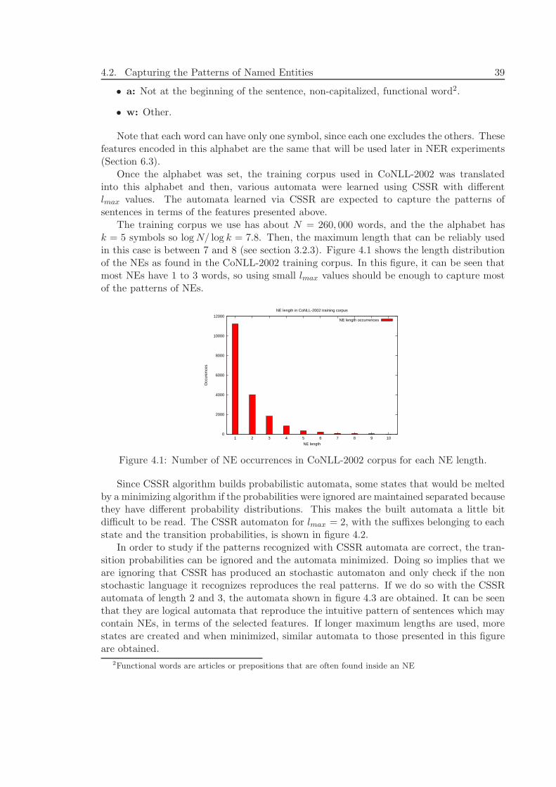
4.2. Capturing the Patterns of Named Entities 39
• a: Not at the beginning of the sentence, non-capitalized, functional word2.
• w: Other.
Note that each word can have only one symbol, since each one excludes the others. Thesefeatures encoded in this alphabet are the same that will be used later in NER experiments(Section 6.3).
Once the alphabet was set, the training corpus used in CoNLL-2002 was translatedinto this alphabet and then, various automata were learned using CSSR with differentlmax values. The automata learned via CSSR are expected to capture the patterns ofsentences in terms of the features presented above.
The training corpus we use has about N = 260, 000 words, and the the alphabet hask = 5 symbols so log N/ log k = 7.8. Then, the maximum length that can be reliably usedin this case is between 7 and 8 (see section 3.2.3). Figure 4.1 shows the length distributionof the NEs as found in the CoNLL-2002 training corpus. In this figure, it can be seen thatmost NEs have 1 to 3 words, so using small lmax values should be enough to capture mostof the patterns of NEs.
0
2000
4000
6000
8000
10000
12000
1 2 3 4 5 6 7 8 9 10
Occ
uren
ces
NE length
NE length in CoNLL-2002 training corpus
NE length occurrences
Figure 4.1: Number of NE occurrences in CoNLL-2002 corpus for each NE length.
Since CSSR algorithm builds probabilistic automata, some states that would be meltedby a minimizing algorithm if the probabilities were ignored are maintained separated becausethey have different probability distributions. This makes the built automata a little bitdifficult to be read. The CSSR automaton for lmax = 2, with the suffixes belonging to eachstate and the transition probabilities, is shown in figure 4.2.
In order to study if the patterns recognized with CSSR automata are correct, the tran-sition probabilities can be ignored and the automata minimized. Doing so implies that weare ignoring that CSSR has produced an stochastic automaton and only check if the nonstochastic language it recognizes reproduces the real patterns. If we do so with the CSSRautomata of length 2 and 3, the automata shown in figure 4.3 are obtained. It can be seenthat they are logical automata that reproduce the intuitive pattern of sentences which maycontain NEs, in terms of the selected features. If longer maximum lengths are used, morestates are created and when minimized, similar automata to those presented in this figureare obtained.
2Functional words are articles or prepositions that are often found inside an NE
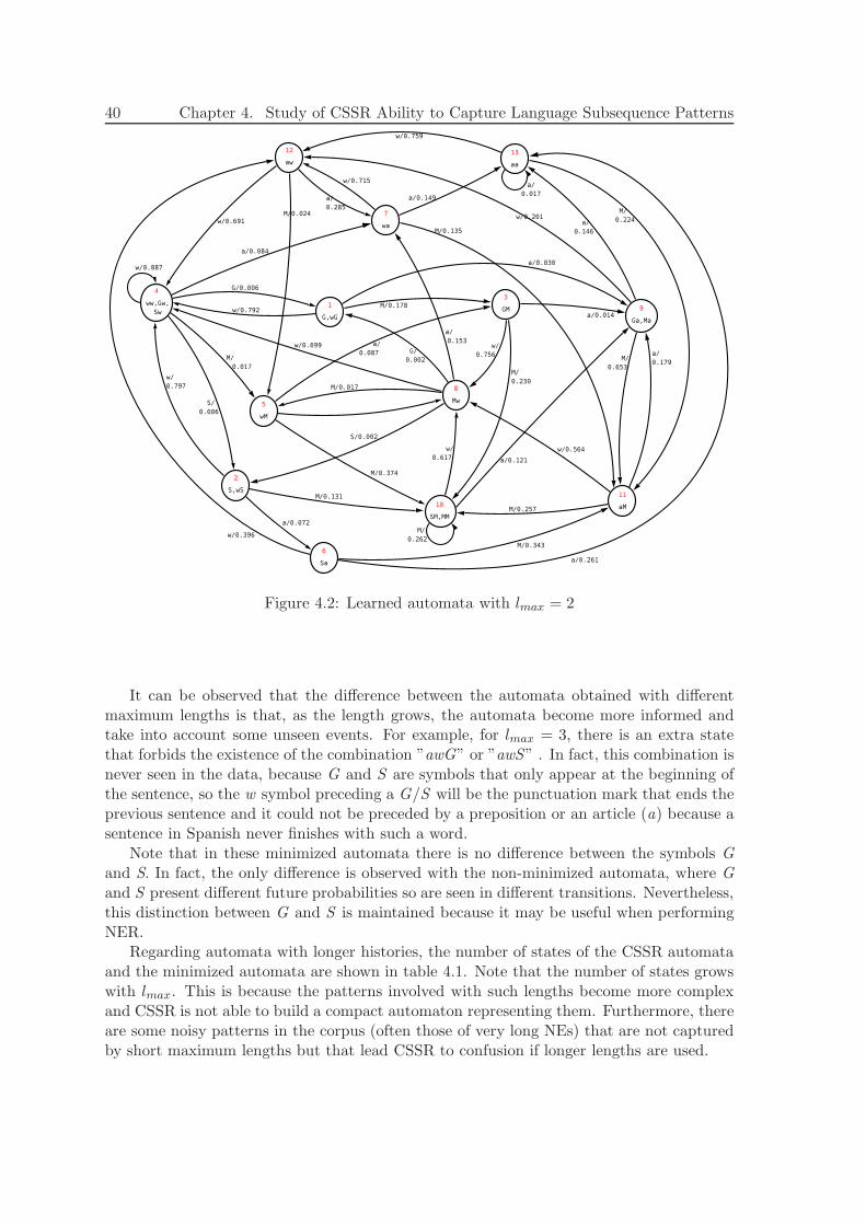
40 Chapter 4. Study of CSSR Ability to Capture Language Subsequence Patterns
Figure 4.2: Learned automata with lmax = 2
It can be observed that the difference between the automata obtained with differentmaximum lengths is that, as the length grows, the automata become more informed andtake into account some unseen events. For example, for lmax = 3, there is an extra statethat forbids the existence of the combination ”awG” or ”awS” . In fact, this combination isnever seen in the data, because G and S are symbols that only appear at the beginning ofthe sentence, so the w symbol preceding a G/S will be the punctuation mark that ends theprevious sentence and it could not be preceded by a preposition or an article (a) because asentence in Spanish never finishes with such a word.
Note that in these minimized automata there is no difference between the symbols Gand S. In fact, the only difference is observed with the non-minimized automata, where Gand S present different future probabilities so are seen in different transitions. Nevertheless,this distinction between G and S is maintained because it may be useful when performingNER.
Regarding automata with longer histories, the number of states of the CSSR automataand the minimized automata are shown in table 4.1. Note that the number of states growswith lmax. This is because the patterns involved with such lengths become more complexand CSSR is not able to build a compact automaton representing them. Furthermore, thereare some noisy patterns in the corpus (often those of very long NEs) that are not capturedby short maximum lengths but that lead CSSR to confusion if longer lengths are used.
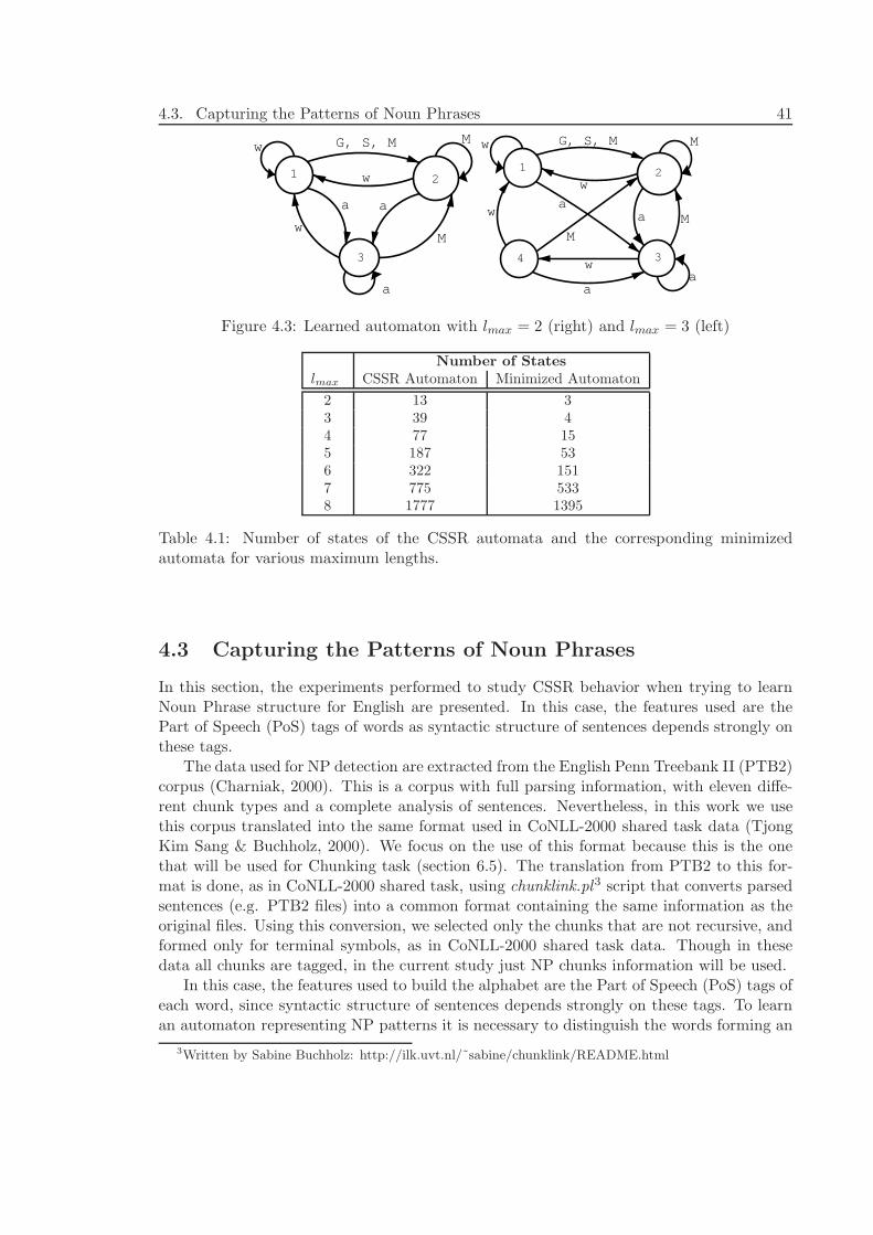
4.3. Capturing the Patterns of Noun Phrases 41
a a
Mw
w
1 2
3
M
a
G, S, M
w
G, S, M
4
a Mw
w
1 2
a
M
3
aw
a
w
M
Figure 4.3: Learned automaton with lmax = 2 (right) and lmax = 3 (left)
Number of States
lmax CSSR Automaton Minimized Automaton
2 13 33 39 44 77 155 187 536 322 1517 775 5338 1777 1395
Table 4.1: Number of states of the CSSR automata and the corresponding minimizedautomata for various maximum lengths.
4.3 Capturing the Patterns of Noun Phrases
In this section, the experiments performed to study CSSR behavior when trying to learnNoun Phrase structure for English are presented. In this case, the features used are thePart of Speech (PoS) tags of words as syntactic structure of sentences depends strongly onthese tags.
The data used for NP detection are extracted from the English Penn Treebank II (PTB2)corpus (Charniak, 2000). This is a corpus with full parsing information, with eleven diffe-rent chunk types and a complete analysis of sentences. Nevertheless, in this work we usethis corpus translated into the same format used in CoNLL-2000 shared task data (TjongKim Sang & Buchholz, 2000). We focus on the use of this format because this is the onethat will be used for Chunking task (section 6.5). The translation from PTB2 to this for-mat is done, as in CoNLL-2000 shared task, using chunklink.pl3 script that converts parsedsentences (e.g. PTB2 files) into a common format containing the same information as theoriginal files. Using this conversion, we selected only the chunks that are not recursive, andformed only for terminal symbols, as in CoNLL-2000 shared task data. Though in thesedata all chunks are tagged, in the current study just NP chunks information will be used.
In this case, the features used to build the alphabet are the Part of Speech (PoS) tags ofeach word, since syntactic structure of sentences depends strongly on these tags. To learnan automaton representing NP patterns it is necessary to distinguish the words forming an
3Written by Sabine Buchholz: http://ilk.uvt.nl/˜sabine/chunklink/README.html
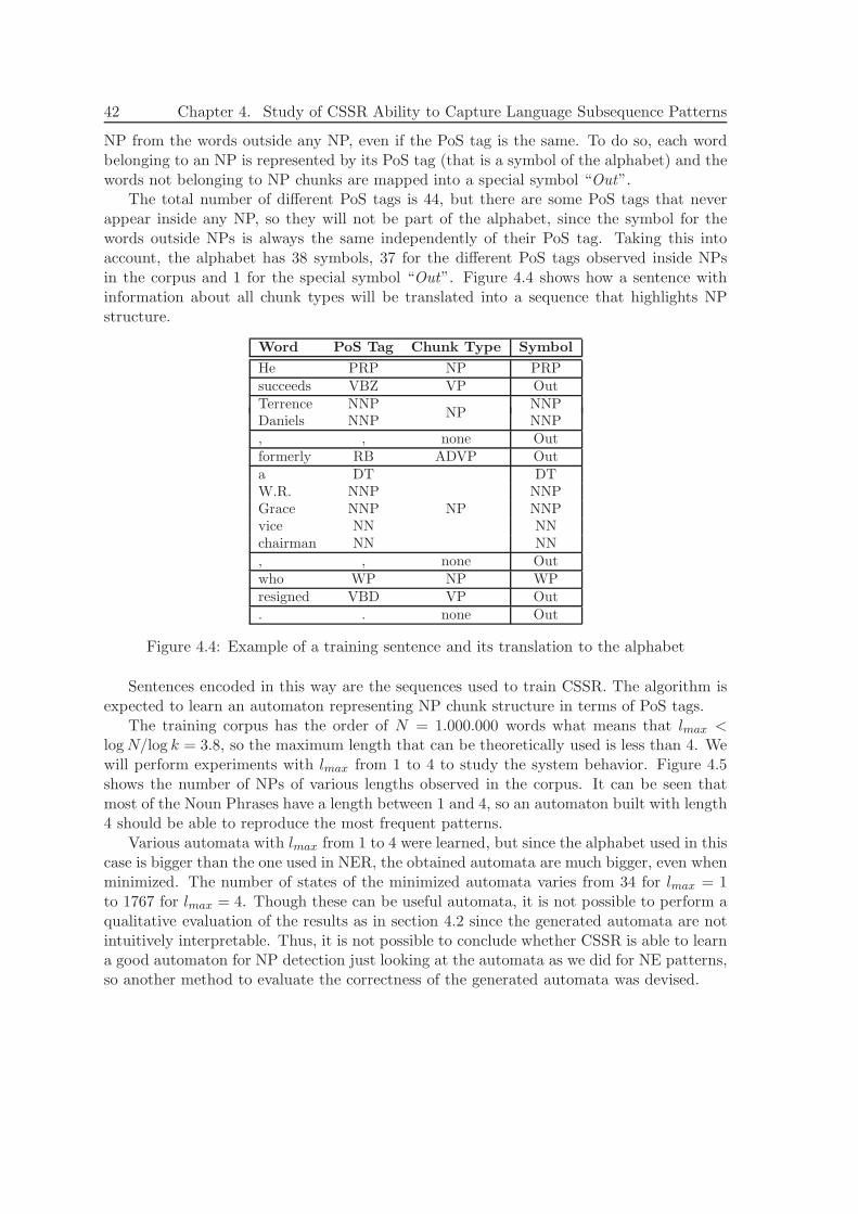
42 Chapter 4. Study of CSSR Ability to Capture Language Subsequence Patterns
NP from the words outside any NP, even if the PoS tag is the same. To do so, each wordbelonging to an NP is represented by its PoS tag (that is a symbol of the alphabet) and thewords not belonging to NP chunks are mapped into a special symbol “Out”.
The total number of different PoS tags is 44, but there are some PoS tags that neverappear inside any NP, so they will not be part of the alphabet, since the symbol for thewords outside NPs is always the same independently of their PoS tag. Taking this intoaccount, the alphabet has 38 symbols, 37 for the different PoS tags observed inside NPsin the corpus and 1 for the special symbol “Out”. Figure 4.4 shows how a sentence withinformation about all chunk types will be translated into a sequence that highlights NPstructure.
Word PoS Tag Chunk Type Symbol
He PRP NP PRPsucceeds VBZ VP OutTerrence NNP NNPDaniels NNP
NPNNP
, , none Outformerly RB ADVP Outa DT DTW.R. NNP NNPGrace NNP NP NNPvice NN NNchairman NN NN, , none Outwho WP NP WPresigned VBD VP Out. . none Out
Figure 4.4: Example of a training sentence and its translation to the alphabet
Sentences encoded in this way are the sequences used to train CSSR. The algorithm isexpected to learn an automaton representing NP chunk structure in terms of PoS tags.
The training corpus has the order of N = 1.000.000 words what means that lmax <log N/log k = 3.8, so the maximum length that can be theoretically used is less than 4. Wewill perform experiments with lmax from 1 to 4 to study the system behavior. Figure 4.5shows the number of NPs of various lengths observed in the corpus. It can be seen thatmost of the Noun Phrases have a length between 1 and 4, so an automaton built with length4 should be able to reproduce the most frequent patterns.
Various automata with lmax from 1 to 4 were learned, but since the alphabet used in thiscase is bigger than the one used in NER, the obtained automata are much bigger, even whenminimized. The number of states of the minimized automata varies from 34 for lmax = 1to 1767 for lmax = 4. Though these can be useful automata, it is not possible to perform aqualitative evaluation of the results as in section 4.2 since the generated automata are notintuitively interpretable. Thus, it is not possible to conclude whether CSSR is able to learna good automaton for NP detection just looking at the automata as we did for NE patterns,so another method to evaluate the correctness of the generated automata was devised.
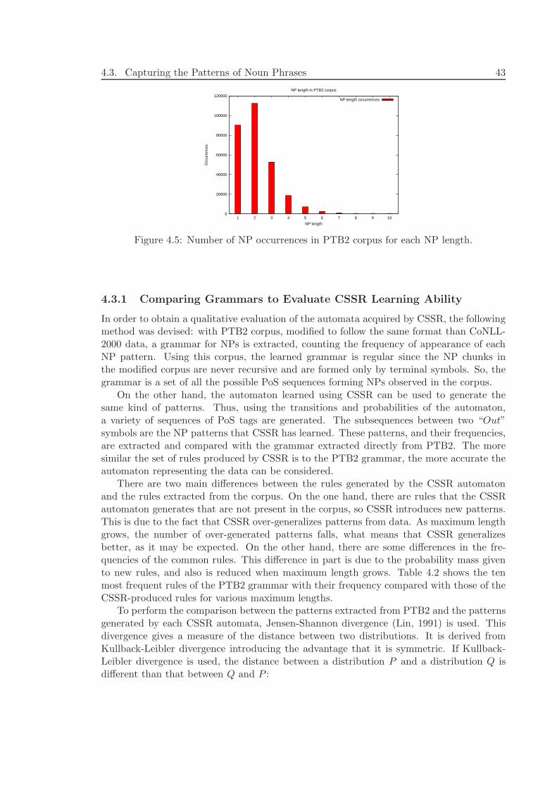
4.3. Capturing the Patterns of Noun Phrases 43
0
20000
40000
60000
80000
100000
120000
1 2 3 4 5 6 7 8 9 10
Occ
uren
ces
NP length
NP length in PTB2 corpus
NP length occurrences
Figure 4.5: Number of NP occurrences in PTB2 corpus for each NP length.
4.3.1 Comparing Grammars to Evaluate CSSR Learning Ability
In order to obtain a qualitative evaluation of the automata acquired by CSSR, the followingmethod was devised: with PTB2 corpus, modified to follow the same format than CoNLL-2000 data, a grammar for NPs is extracted, counting the frequency of appearance of eachNP pattern. Using this corpus, the learned grammar is regular since the NP chunks inthe modified corpus are never recursive and are formed only by terminal symbols. So, thegrammar is a set of all the possible PoS sequences forming NPs observed in the corpus.
On the other hand, the automaton learned using CSSR can be used to generate thesame kind of patterns. Thus, using the transitions and probabilities of the automaton,a variety of sequences of PoS tags are generated. The subsequences between two “Out”symbols are the NP patterns that CSSR has learned. These patterns, and their frequencies,are extracted and compared with the grammar extracted directly from PTB2. The moresimilar the set of rules produced by CSSR is to the PTB2 grammar, the more accurate theautomaton representing the data can be considered.
There are two main differences between the rules generated by the CSSR automatonand the rules extracted from the corpus. On the one hand, there are rules that the CSSRautomaton generates that are not present in the corpus, so CSSR introduces new patterns.This is due to the fact that CSSR over-generalizes patterns from data. As maximum lengthgrows, the number of over-generated patterns falls, what means that CSSR generalizesbetter, as it may be expected. On the other hand, there are some differences in the fre-quencies of the common rules. This difference in part is due to the probability mass givento new rules, and also is reduced when maximum length grows. Table 4.2 shows the tenmost frequent rules of the PTB2 grammar with their frequency compared with those of theCSSR-produced rules for various maximum lengths.
To perform the comparison between the patterns extracted from PTB2 and the patternsgenerated by each CSSR automata, Jensen-Shannon divergence (Lin, 1991) is used. Thisdivergence gives a measure of the distance between two distributions. It is derived fromKullback-Leibler divergence introducing the advantage that it is symmetric. If Kullback-Leibler divergence is used, the distance between a distribution P and a distribution Q isdifferent than that between Q and P :
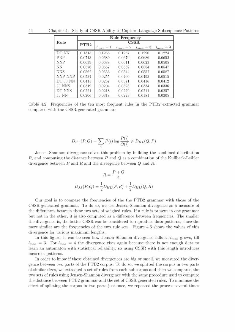
44 Chapter 4. Study of CSSR Ability to Capture Language Subsequence Patterns
Rule
Rule Frequency
PTB2CSSR
lmax = 1 lmax = 2 lmax = 3 lmax = 4
DT NN 0.1315 0.1256 0.1267 0.1290 0.1224PRP 0.0713 0.0689 0.0679 0.0686 0.0652NNP 0.0639 0.0688 0.0611 0.0623 0.0505NN 0.0576 0.0657 0.0562 0.0584 0.0547NNS 0.0562 0.0553 0.0544 0.0557 0.0587NNP NNP 0.0534 0.0255 0.0460 0.0493 0.0515DT JJ NN 0.0415 0.0267 0.0371 0.0416 0.0412JJ NNS 0.0319 0.0204 0.0325 0.0334 0.0336DT NNS 0.0221 0.0218 0.0229 0.0211 0.0257JJ NN 0.0206 0.0318 0.0223 0.0181 0.0205
Table 4.2: Frequencies of the ten most frequent rules in the PTB2 extracted grammarcompared with the CSSR-generated grammars
DKL(P,Q) =∑
i
P (i) logP (i)
Q(i)6= DKL(Q,P )
Jensen-Shannon divergence solves this problem by building the combined distributionR, and computing the distance between P and Q as a combination of the Kullback-Leiblerdivergence between P and R and the divergence between Q and R:
R =P + Q
2
DJS(P,Q) =1
2DKL(P,R) +
1
2DKL(Q,R)
Our goal is to compare the frequencies of the the PTB2 grammar with those of theCSSR generated grammar. To do so, we use Jensen-Shannon divergence as a measure ofthe differences between these two sets of weighed rules. If a rule is present in one grammarbut not in the other, it is also computed as a difference between frequencies. The smallerthe divergence is, the better CSSR can be considered to reproduce data patterns, since themore similar are the frequencies of the two rule sets. Figure 4.6 shows the values of thisdivergence for various maximum lengths.
In this figure, it can be seen how Jensen Shannon divergence falls as lmax grows, tilllmax = 3. For lmax = 4 the divergence rises again because there is not enough data tolearn an automaton with statistical reliability, so using CSSR with this length introducesincorrect patterns.
In order to know if these obtained divergences are big or small, we measured the diver-gence between two parts of the PTB2 corpus. To do so, we splitted the corpus in two partsof similar sizes, we extracted a set of rules from each subcorpus and then we compared thetwo sets of rules using Jensen-Shannon divergence with the same procedure used to computethe distance between PTB2 grammar and the set of CSSR generated rules. To minimize theeffect of splitting the corpus in two parts just once, we repeated the process several times
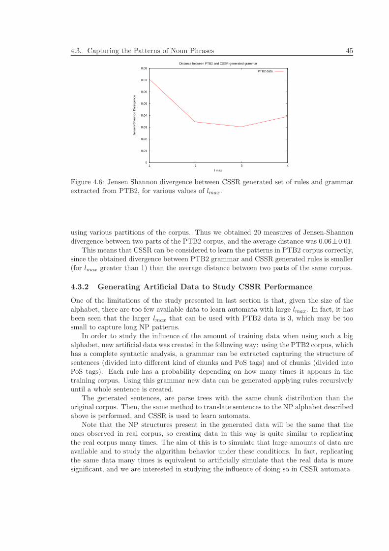
4.3. Capturing the Patterns of Noun Phrases 45
0
0.01
0.02
0.03
0.04
0.05
0.06
0.07
0.08
1 2 3 4
Jens
en-S
hann
on D
iver
genc
e
l max
Distance between PTB2 and CSSR-generated grammar
PTB2 data
Figure 4.6: Jensen Shannon divergence between CSSR generated set of rules and grammarextracted from PTB2, for various values of lmax.
using various partitions of the corpus. Thus we obtained 20 measures of Jensen-Shannondivergence between two parts of the PTB2 corpus, and the average distance was 0.06±0.01.
This means that CSSR can be considered to learn the patterns in PTB2 corpus correctly,since the obtained divergence between PTB2 grammar and CSSR generated rules is smaller(for lmax greater than 1) than the average distance between two parts of the same corpus.
4.3.2 Generating Artificial Data to Study CSSR Performance
One of the limitations of the study presented in last section is that, given the size of thealphabet, there are too few available data to learn automata with large lmax. In fact, it hasbeen seen that the larger lmax that can be used with PTB2 data is 3, which may be toosmall to capture long NP patterns.
In order to study the influence of the amount of training data when using such a bigalphabet, new artificial data was created in the following way: using the PTB2 corpus, whichhas a complete syntactic analysis, a grammar can be extracted capturing the structure ofsentences (divided into different kind of chunks and PoS tags) and of chunks (divided intoPoS tags). Each rule has a probability depending on how many times it appears in thetraining corpus. Using this grammar new data can be generated applying rules recursivelyuntil a whole sentence is created.
The generated sentences, are parse trees with the same chunk distribution than theoriginal corpus. Then, the same method to translate sentences to the NP alphabet describedabove is performed, and CSSR is used to learn automata.
Note that the NP structures present in the generated data will be the same that theones observed in real corpus, so creating data in this way is quite similar to replicatingthe real corpus many times. The aim of this is to simulate that large amounts of data areavailable and to study the algorithm behavior under these conditions. In fact, replicatingthe same data many times is equivalent to artificially simulate that the real data is moresignificant, and we are interested in studying the influence of doing so in CSSR automata.
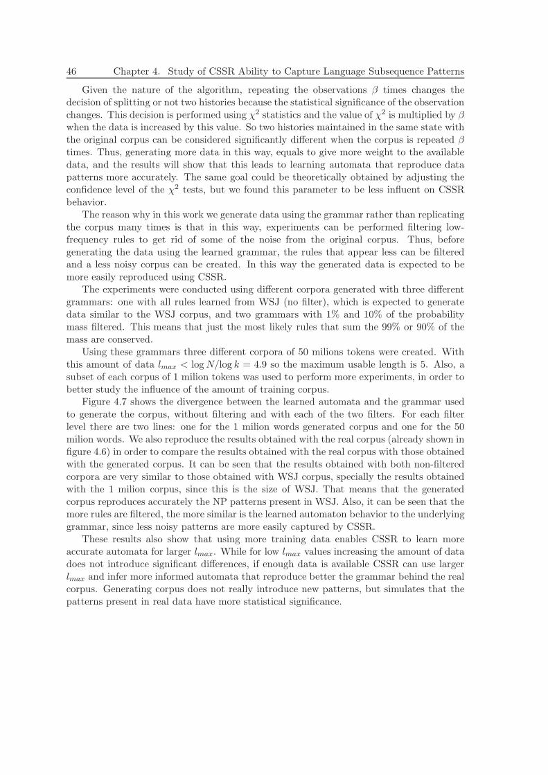
46 Chapter 4. Study of CSSR Ability to Capture Language Subsequence Patterns
Given the nature of the algorithm, repeating the observations β times changes thedecision of splitting or not two histories because the statistical significance of the observationchanges. This decision is performed using χ2 statistics and the value of χ2 is multiplied by βwhen the data is increased by this value. So two histories maintained in the same state withthe original corpus can be considered significantly different when the corpus is repeated βtimes. Thus, generating more data in this way, equals to give more weight to the availabledata, and the results will show that this leads to learning automata that reproduce datapatterns more accurately. The same goal could be theoretically obtained by adjusting theconfidence level of the χ2 tests, but we found this parameter to be less influent on CSSRbehavior.
The reason why in this work we generate data using the grammar rather than replicatingthe corpus many times is that in this way, experiments can be performed filtering low-frequency rules to get rid of some of the noise from the original corpus. Thus, beforegenerating the data using the learned grammar, the rules that appear less can be filteredand a less noisy corpus can be created. In this way the generated data is expected to bemore easily reproduced using CSSR.
The experiments were conducted using different corpora generated with three differentgrammars: one with all rules learned from WSJ (no filter), which is expected to generatedata similar to the WSJ corpus, and two grammars with 1% and 10% of the probabilitymass filtered. This means that just the most likely rules that sum the 99% or 90% of themass are conserved.
Using these grammars three different corpora of 50 milions tokens were created. Withthis amount of data lmax < log N/log k = 4.9 so the maximum usable length is 5. Also, asubset of each corpus of 1 milion tokens was used to perform more experiments, in order tobetter study the influence of the amount of training corpus.
Figure 4.7 shows the divergence between the learned automata and the grammar usedto generate the corpus, without filtering and with each of the two filters. For each filterlevel there are two lines: one for the 1 milion words generated corpus and one for the 50milion words. We also reproduce the results obtained with the real corpus (already shown infigure 4.6) in order to compare the results obtained with the real corpus with those obtainedwith the generated corpus. It can be seen that the results obtained with both non-filteredcorpora are very similar to those obtained with WSJ corpus, specially the results obtainedwith the 1 milion corpus, since this is the size of WSJ. That means that the generatedcorpus reproduces accurately the NP patterns present in WSJ. Also, it can be seen that themore rules are filtered, the more similar is the learned automaton behavior to the underlyinggrammar, since less noisy patterns are more easily captured by CSSR.
These results also show that using more training data enables CSSR to learn moreaccurate automata for larger lmax. While for low lmax values increasing the amount of datadoes not introduce significant differences, if enough data is available CSSR can use largerlmax and infer more informed automata that reproduce better the grammar behind the realcorpus. Generating corpus does not really introduce new patterns, but simulates that thepatterns present in real data have more statistical significance.
4.4. Discussion 47
0
0.01
0.02
0.03
0.04
0.05
0.06
0.07
0.08
1 2 3 4 5
Jens
en-S
hann
on D
iver
genc
e
l max
Distance between PTB2 and CSSR-generated grammar
PTB2 data1 milion words, no filter
50 milion words, no filter1 milion words, filter 1%
50 milion words, filter 1%1 milion words, filter 10%
50 milion words, filter 10%
Figure 4.7: Jensen Shannon divergence between CSSR generated set of rules with a ge-nerated corpus and grammar extracted from PTB2, for various values of lmax when usingvarious filter levels of the grammar
4.4 Discussion
Considering the results, we can conclude that CSSR is a good method for learning patterns,even quite complicated patterns as those of NPs, but it is highly depending on the amountof available data. For each process, there is a necessary lmax value to be able to capturethe patterns, and if this value is high, large corpus will be necessary. Furthermore, sincethe minimum amount of data necessary to learn a good automaton with a determined lmax
depends exponentially on the alphabet size (N > klmax), to be able to increase lmax in 1, itwould be necessary to multiply the data size by the size of the alphabet k.
For NE patterns, it has been seen that the automaton learned using CSSR is intuitiveand captures the patterns of sentences in terms of the designed alphabet. This is partlydue to the fact that for this task the alphabet is quite small, so it is easier to build anunderstandable automaton than in NP task.
For NP detection, the linguistic meaning of CSSR generated automaton can not beintuitively understood, but that does not mean that it does not reproduces NP patternscorrectly. The automaton can be qualitatively studied comparing the patterns that itgenerates with the patterns observed in the training corpus. The more similar are the twosets of patterns, the better is CSSR reproducing the patterns of the task. This comparisonshows that for real data CSSR can learn better patterns as lmax grows but due to thelimited amount of available data, for lmax = 4 the divergence rises again, since there is notenough data to learn an automaton reproducing corpus patterns with this length. So, the
48 Chapter 4. Study of CSSR Ability to Capture Language Subsequence Patterns
performance of the system is limited by the size of the training corpus.The generated and not filtered data can be considered equivalent to the real corpus.
Also, it can be seen that when using a big amount of generated data the performance isbetter than for the real data since the system can deal with longer lmax . When using smalllmax the difference between using 1 milion or 50 milion data is not significant. Furthermore,as it was expected, as the number of filtered rules grows, the divergence falls, being reallysmall when lmax grows. This means that the easier the patterns to learn are, the betterthey are captured by CSSR. In the case of filtered rules, the system also performs betterwith large lmax if enough data is available.
4.5 Conclusions of this Chapter
This chapter has presented a study of how CSSR is able to capture some patterns in lan-guage. It has been seen that this algorithm can learn an automaton representing a processif there is enough data available without, or if the process is simple enough. The influenceof the amount of data and the noise level in the generated automaton has been qualitativelystudied.
The main conclusion of this chapter is that CSSR can learn correctly the patterns ofsequential data, specially if the data is not very noisy, but that it is highly dependent on theamount of data, the size of the alphabet and lmax value. Furthermore, this dependency isexponential, so to increase a little bit the performance of the system, it would be necessaryto magnify the amount of data. CSSR has been proved also to be useful when dealing withsystems with smaller alphabets –as in other applications of CSSR such as those presentedin (Varn & Crutchfield, 2004; Clarke et al., 2003; Cointet et al., 2007)– but to use it insystems with lots of features to be taken into account, as NLP tasks, this could be limitedby the amount of available data.
Nevertheless, since the algorithm has proven to be useful to learn NLP patterns, we thinkit is interesting to apply it to annotating tasks in order to see if the characteristics thatmake CSSR theoretically more powerful than other techniques such as HMM or VLMM,are reflected in the obtained results.
In fact, one of the main limitations of CSSR is that it is useful to learn patterns, but itis not directly prepared to introduce hidden information and to perform annotating tasks.Chapter 5 presents our proposal to introduce this hidden information into the system, andfolowing chapters will present the results obtained with this technique.
CHAPTER 5
Adapting CSSR to Perform Annotation Tasks
So far, this work has focused on the performance of CSSR when learning sentence patternsin terms of some selected sets of features encoded into the alphabet. It has been seen thatCSSR is able to capture the patterns underlying some language subsequences. Nevertheless,for NLP tasks, it is necessary to develop systems able to annotate new sentences. This is,given a new sentence, the system has to detect the subsequences we are interested in. Inthe case of Noun Phrase (NP) detection, for example, we would have sentences with theirPoS, without the information about which words form an NP chunk, and the system shoulddetect the NPs of this sentence. To perform this annotation task with CSSR, it is necessaryto encode into the system the hidden information about where certain subsequences beginand end. Originally, CSSR is not conceived to encode this hidden information, so in thischapter we propose an approach to adapt CSSR to include and use it to annotate newsentences.
In this approach, we focus on tasks where some subsequences of words, with specificproperties, have to be detected. Some examples of this kind of task are Named EntityRecognition (NER) and Chunking. For the NER task, the subsequences we are interestedin are Named Entities (NE) and for Chunking, they are the different kind of phrases. Asa general way of referring to these subsequences we are interested in detecting, we will callthem “chunks”, understanding this concept as the wide idea of a subsequence of wordsbelonging to a class. Also, the task of determining subsequences of words will be referredto as “chunk detection”.
The general idea of our approach is to use CSSR to learn an automaton representingthe chunk structure taking into account the hidden information that says where each sub-sequence begins or ends. Once the automaton is learned with this information, it can beapplied to detect subsequences in untagged text.
This approach and its application to various NLP tasks has been published in (Padro& Padro, 2005a; Padro & Padro, 2005b; Padro & Padro, 2005c).
49
50 Chapter 5. Adapting CSSR to Perform Annotation Tasks
5.1 Representing the Hidden Information
First of all, we need to state a way of representing the hidden information we want tointroduce into the system. Since we are interested in subsequence annotation tasks, thishidden information is simply if a word belongs or not to a determined chunk or subsequence.
There are many different possible approaches to tagging this kind of structures (TjongKim Sang & Veenstra, 1999) one of the most widely used is the “B-I-O” approach (Ramshaw& Marcus, 1995): each word has a B, I or O tag, being B the tag for a word where asubsequence or chunk begins, I when the word is part of a chunk but not the beginning,and O the tag for the words not belonging to any subsequence.
Another approach often used to annotate subsequences, specially syntactic chunks, con-sists of using brackets to determine their boundaries (Church, 1988): the first word in achunk has an opening bracket “[” and the last one a closing bracket “]”. All the wordsinside two consecutive opening and closing brackets belong to the same chunk.
There are other ways of representing chunks but they are mainly modifications or com-binations of these two main methods. For a specific review on them, see (Tjong Kim Sang& Veenstra, 1999).
In this work, we will use the “B-I-O” approach, since it is one of the most widely used inall tasks regarding subsequence detection, and also because our experiments will use the dataof CoNLL 2000 and 2002 shared tasks1 that follow this “B-I-O” approach. Nevertheless,the proposed approach could be used with the other possible annotation systems, since theidea is general enough.
5.2 Learning the Automaton with the Hidden Information
To learn the automaton that must reproduce a chunk structure, different information aboutthe words is used, as it has been seen in chapter 4 where various alphabets have beencreated for learning NE and NP patterns. Obviously, the used information depends onthe specific kind of subsequence we want to detect, and can be for example orthographic,morpho-syntactic, about the position in the sentence, etc. Using the chosen features, thealphabet of the automaton is built as a closed set of symbols, and the words in a sentenceare translated into this alphabet. The sentences in the train corpus translated in such a waywill be the sequence that we use to learn the automaton via CSSR. The learned automatonwill reproduce the sequence behavior in terms of the chosen features.
This is conceptually equivalent to the process performed in chapter 4, but now we needto introduce the hidden information about if a word is part of a determined chunk or not.To do so, we propose to introduce into the alphabet the information of the chunk tag (B,I or O) available in the supervised training corpus. Thus, the correct tag is part of thealphabet symbol that represents each word and is taken into account when building theautomaton.
More specifically, we consider two different parts of the alphabet. First of all, thereis the part that can be built without any hidden information, that we will call the visiblealphabet : Σ = {s1, s2, ..., sk}. This alphabet corresponds to the symbols associated to thevisible features of the words and does not take into account any hidden information. That
1CoNLL 2000 shared task was devoted to text chunking, and CoNLL 2002 shared task approached NamedEntity Recognition and Classification
5.3. Using the Learned Automaton to Annotate Language Subsequences 51
means that we can translate a text into this alphabet even if the chunks in that text arenot tagged. The alphabets used in chapter 4 are purely visible alphabets.
Once this alphabet is defined, to introduce the hidden information, we create anotheralphabet, to which we will refer to as complet alphabet, that combines each possible symbolin the visible alphabet with each possible hidden tag: ΣBIO = {s1
B , s1I , s
1O, ..., sk
B , skI , s
kO}.
Thus, the alphabet size has been multiplied by the number of hidden tags, in our approach,the complet alphabet is three times bigger than the visible alphabet.
Once this complet alphabet is defined, all the sentences in the training corpus, thatcontain the correct B-I-O tag for each word, can be translated into this alphabet and CSSRis used to learn an automaton with these data. Then, the learned automaton will encodein its transitions not only the information about the relevant features for the task, but alsothe information about the probabilities of each kind of word having the B, I or O tag ineach determined context. Thus, we can later use this automaton to compute the best pathfor a sequence and use it to annotate chunks in a new text.
5.2.1 An Example
To better illustrate our proposal to annotate chunks in a sentence using CSSR algorithm,here we present an example of annotating Named Entities. Let’s suppose an approach wherethe features used are the same presented in 4.2. In this case, the alphabet will consist offifteen symbols, which are the possible combinations of those five visible symbols with thethree possible NE tags (GB , GI , GO, SB , SI , SO, MB , MI , GB , GI , GO, SB, SI , SO, MB,MI , MO, aB , aI , aO, wB, wI , wO ). Each word will be translated into one of these symbolsdepending on the features it presents.
Once the data are properly translated into the alphabet, the automaton is built usingCSSR. Figure 5.2 shows a possible (not real) automaton with this alphabet. In this figure,the probabilities are not shown to facilitate the reading but the automaton learned byCSSR would have a probability assigned to each possible transition with each symbol in thealphabet. Note that there are nonexistent transitions (GI and SI never occur, for example).This transitions will have a null probability and will go to a sink state.
This is a simple example, where only sequences such as ...wOwOMBaIMBwO... or...wOGBMBwO... are considered. This automaton forbids sequences such as ...wOMBaIMO...that are very infrequent in real language but may still be found in a real training corpus.In a real automaton learned with CSSR much more transitions and states will be present,since the automaton reproduces all the patterns seen in the corpus even the very infrequentones. Furthermore, as the algorithm builds the causal states depending on the probabilitydistribution for the future, the built automata tend to be bigger because states with similarbehavior regarding the NE structure are maintained separately because they have differentprobability distributions.
5.3 Using the Learned Automaton to Annotate Language
Subsequences
When a concrete kind of subsequence in a sentence has to be annotated, the informationabout the correct chunk tag is not available, so there are several possible alphabet symbolsfor that word. It is possible to know only the part of the translation that depends on theword or sentence features, so we can know the corresponding visible alphabet symbol (si),
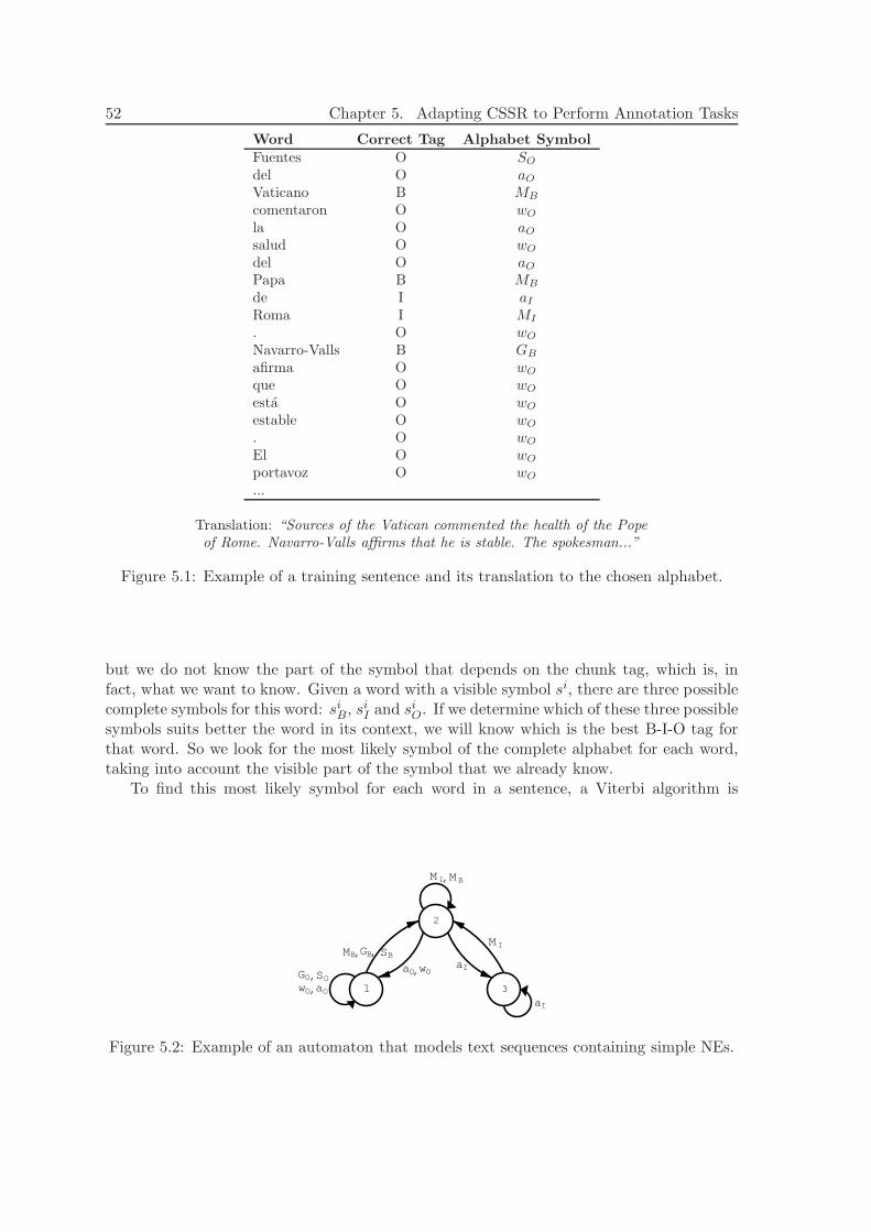
52 Chapter 5. Adapting CSSR to Perform Annotation Tasks
Word Correct Tag Alphabet Symbol
Fuentes O SO
del O aO
Vaticano B MB
comentaron O wO
la O aO
salud O wO
del O aO
Papa B MB
de I aI
Roma I MI
. O wO
Navarro-Valls B GB
afirma O wO
que O wO
esta O wO
estable O wO
. O wO
El O wO
portavoz O wO
...
Translation: “Sources of the Vatican commented the health of the Popeof Rome. Navarro-Valls affirms that he is stable. The spokesman...”
Figure 5.1: Example of a training sentence and its translation to the chosen alphabet.
but we do not know the part of the symbol that depends on the chunk tag, which is, infact, what we want to know. Given a word with a visible symbol si, there are three possiblecomplete symbols for this word: si
B, siI and si
O. If we determine which of these three possiblesymbols suits better the word in its context, we will know which is the best B-I-O tag forthat word. So we look for the most likely symbol of the complete alphabet for each word,taking into account the visible part of the symbol that we already know.
To find this most likely symbol for each word in a sentence, a Viterbi algorithm is
2
1 3
GB BSBM
,, ,
, ,
aO
aOOSGO
Ow
Ow
,
aI
aI
M I
M I M B
Figure 5.2: Example of an automaton that models text sequences containing simple NEs.
5.4. Managing Unseen Transitions 53
applied. That is, for each word in a sentence, the possible states the automaton could reachif the current word had the tag B, I, or O (that is, if the symbol was si
B, siI or si
O), andthe probabilities of these paths are computed. Then, only the highest probability for eachtag is recorded. That means that for each word, the best path for this word having eachtag is stored. At the end of the sentence, the best probability is chosen and the optimalpath is backwards recovered. In this way, the most likely sequence of complete symbols, soof B-I-O tags for each word in the sentence is obtained. There are some forbidden paths,which are those that lead to the OI tag combination. The paths including this combinationare pruned out since they include incorrect tag combinations.
Returning to the example presented in 5.2.1, let’s see how the automaton presented infigure 5.2 will perform the NE-annotation of a sentence. Most of the time the automatonwill stay in the state 1, with input symbols w, as most words will have this symbol. In thisstate, all w words will be tagged with an O, since the symbols wI and wO do not have anytransition from this state. When a G symbol comes, the automaton will transit to state2, supposing that the correct tag for that symbol is B and to state 1, supposing that thecorrect tag is O. Each of these two paths will have different probability depending on theprobabilities assigned to each transition. If after that symbol, a preposition is seen (visiblesymbol a), the system has three possibilities: go from state 2 to 3 with an I tag, from 2 to 1with an O tag, or from 1 to 1 also with an O tag. In the last case, only the path with higherprobability will be recorded, because only the best path for each B-I-O tag is recorded ineach instant. This process goes on until the end of a sentence, when the most likely path ischosen and the tags for each word are recovered.
5.4 Managing Unseen Transitions
When performing the annotation of subsequences in a text, it is possible to find symbolsequences that have not been seen in the training corpus. It can imply that there is notransition available for the studied symbol in the current state. Since there are differenthistories grouped in the same state, sometimes there will be an available transition deter-mined by another suffix in the state, but if this does not happen, the automaton will fall ina sink state, which receives all the unseen transitions. This state can be seen as the statethat contains all the unseen suffixes.
When the system transitions to the sink state, we are interested on not loosing thestudied path, so the probability of the transition from the current state to the sink state isnot considered zero but smoothed to a small value using Lidstone’s law (Manning & Schutze,1998). Actually, the only sequences that have null probability are those that contain a suffixwith the forbidden tag combination “OI”, this is, all suffixes of the form si
OsjI .
When the automaton falls in the sink state, it can not follow the input sequence usingstate-to-state transition information because, since the transitions were not seen, they arenot defined. Then, it is necessary to define a method to allow the system to continueannotating the text, and to go out of the sink state as soon as possible. In this work, wepropose two different ways of dealing with the sink state, presented in next sections. Thefirst method consists of waiting for a seen suffix and the second one in looking for suffixessharing the same ending.
54 Chapter 5. Adapting CSSR to Perform Annotation Tasks
Waiting for a Seen Suffix
This first method propose to keep reading the text input and building all possible suffixestill some of the built suffixes is found in an existing state. To do so, when the automatonfalls into sink state, the suffix of length lmax is built concatenating the last lmax−1 symbolswith the next symbol from the input, which is the symbol that made the automaton fallinto the sink state. This first suffix for sure will not be in any state in the automaton, butthen the next symbol (word) of the input is studied creating the new suffix in the same way.Then, a state containing this new suffix is searched over the automaton and, if found, theautomaton goes to this state and continues its normal functioning. If not, the process isrepeated, getting more symbols from the input sequence, until a state containing the newsuffix is found. Note that for each visible symbol taken from the input, three new suffixesare created, one for each possible complete symbol (combination of the visible symbol withthe B-I-O tags).
This may cause skipping some part of the input, since the suffixes not found in theautomaton are considered to have a smoothed probability so we can not say which is thecorrect tag for them. This is caused by the fact that the text sequence is consideredas a stationary process, and so, when the CSSR-acquired automaton fails, we have toresynchronize it with the input data.
Looking for a Suffix Sharing the Same Ending
Another possibility to fix the problem of falling into the sink state is to study the unseensuffix that has made the automaton evolute to the sink state and look for other suffixessharing the same ending. If the suffixes are long enough, we can consider that shortening alittle bit the history taken into account can not lead to a high loose of information while, onthe other hand, let the system continue its normal functioning without waiting for a seensuffix.
Note that in this case, there could be more than one state sharing the same ending ofthe unseen suffixes. Then, the system considers all the possible states and continues all thepaths from each state and in the next step only the paths with higher probabilities will bekept.
5.5 Validating the Method
A preliminary experiment to validate the proposed approach was performed. The goal ofthis preliminary experiment is to see if CSSR is able to learn correctly the patterns createdby a hand-written automaton and to evaluate the attained performance when using it toannotate new text.
To do so, we focus on Named Entity Recognition task for Spanish, for which FreeLinganalyzer (Carreras et al., 2004; Atserias et al., 2006) has a system that uses a simplehand-built automaton of four states. The alphabet used in this automaton is the same–and encode the same features– than the one presented in 4.2. We use this system to re-annotate both a training and a test corpora, obtaining corpora annotated with a simpleand systematic annotation criteria. Note that now we are not looking for the real NEs, butwe just want to check if CSSR is able to reproduce the behavior of FreeLing automaton,independently of the correctness of the FreeLing tags.
5.6. Conclusions of this Chapter 55
The corpora we use are those of CoNLL-2002 shared task (Tjong Kim Sang, 2002a) forSpanish, that will be also used and better introduced in chapter 6. This data-set containsa training corpus, one corpus for the development of the system and another one for theevaluation. In this case, we will test our system on both the development and evaluationcorpora, since we are not developing a system, just checking the validity of our method.Actually, these experiments could be done with any text, since the manual NE tags arecompletely ignored at this moment and just the FreeLing tags are taken into account.
Thus, these three corpora with the NEs detected by FreeLing analyzer are the data usedto test our proposal for using CSSR at subsequence detection tasks. The vocabulary weuse is the same presented in the example 5.2.1 that combines the visible part of the symbolintroduced in 4.2 with each possible hidden tag: GB , GI , GO, SB, SI , SO, MB , MI , GB ,GI , GO, SB, SI , SO, MB , MI , MO, aB , aI , aO, wB, wI , wO. Since the visible part of thealphabet is the same than the one used by FreeLing NER system, the features taken intoaccount are the same and CSSR is expected to be able to learn automata that reproducescorrectly the behavior of this hand-build NER system.
Using the training corpus annotated with FreeLing translated into the complete alpha-bet, two automata were learned using CSSR algorithm: one for lmax = 2 and one forlmax = 3. Then, these automata were evaluated over both test corpora (also annotatedwith FreeLing) with the method explained in 5.3. The system obtained F1 = 100% whenusing lmax = 2 for both test sets, and using lmax = 3, F1 = 99, 83% for the CoNLL-2002 de-velopment corpus and F1 = 99, 98% for the CoNLL-2002 evaluation corpus were obtained.For lmax = 3, the lost in F1 is due to some missed NEs. In fact the system obtained 100%precision in both cases, but the recall fell a little bit. This lose in the recall, could be due tothe fact that if lmax rises, more training data are necessary to generate a correct automaton.
These results prove that CSSR is able to perfectly acquire the behavior of the FreeLingannotation schema underlying the data. Although this is an easy task, since that schema issimple and systematic, it validates the viability of our adaptation of CSSR from stationary-process acquisition to pattern recognition. In next chapter we will present and discus theperformance of this schema when applied to real data.
5.6 Conclusions of this Chapter
In this chapter, we have presented our approach to use CSSR in NLP annotating tasks. Sofar, we have focused on tasks that imply subsequence detection. The proposed approachconsists basically of introducing the hidden information about where the subsequences beginand end into the alphabet and learn an automaton containing this information. Then, theautomaton can be used to annotate new sentences using a Viterbi algorithm. Also, twomethods for dealing with unseen events when performing the annotating step have beenpresented.
An important issue to take into account is that the fact of introducing the hidden tagsinto the visible alphabet makes the alphabet three times bigger than the visible alphabet.In chapter 4 we have already discussed that one of the limitations of CSSR is that theamount of data necessary to learn a good automaton grows exponentially with the sizeof the alphabet. Now, we are multiplying the alphabet size by three, in respect with theexperiments performed in chapter 4 when no hidden information was taken into account.This means that the amount of necessary data to use CSSR with the same lmax used without

56 Chapter 5. Adapting CSSR to Perform Annotation Tasks
B-I-O information is 3lmax times bigger than what was needed before. If CSSR can learn anaccurate automaton of length l using a training corpus of N = kl words, N ′ = (3k)l = N ∗3l
words will be necessary to perform the annotation task under the B-I-O approach.Next chapter will present the experiments performed with this approach to annotate
Named Entities and to detect the sintactic chunks in a text. Then, at the sight of theresults we will better discuss the limitations of the proposed method and will study theeffect of having a limited amount of data.
CHAPTER 6
Experiments and Results with CSSR in
Annotation Tasks
In this chapter, the performed experiments and the obtained results of applying CSSR toannotation tasks under the approach proposed in chapter 5 are presented.
First of all, we summarize in sections 6.1 and 6.2 the different system configurations thatwe will use and test, as well as the measures and corpora used to determine the performanceof each configuration. Then, we explain in detail the experiments and results with the threeaddressed tasks. The tasks we are interested in are Named Entity Recognition (NER) bothin general and medical domain, and Text Chunking.
Some of the experiments with NER in general domain presented here were published in(Padro & Padro, 2005a; Padro & Padro, 2005c). The application of CSSR to biomedicalNER was presented in a poster at BioLink’07 (Dowdall et al., 2007) and the Chunkingexperiments can be found in (Padro & Padro, 2005b).
6.1 Experimental Settings
So far we have explained the method we use and our proposal to apply it to NLP annotationtasks. We have focused on the main ideas behind the method and we have also explainedwhich are the most important parameters for the algorithm. Nevertheless, when applying itto the real tasks, we found some useful variations of the original system and other parametersthat also could influence the performance of the system. In next sections we review all theseparemeters and enumerate all the different settings that we have used in our experiments.
6.1.1 Maximum Length
As we have already said, one of the main parameters of the CSSR algorithm is the maximumlength lmax the suffixes can reach. All the experiments will be performed with variouslmax values in order to study the influence of this parameter.
57
58 Chapter 6. Experiments and Results with CSSR in Annotation Tasks
6.1.2 Hypothesis Test
Another influent issue is the confidence degree of the hypothesis test and the hypothesistest itself. Our first experiments were performed with χ2 test, and with various values of itsconfidence degree α. But, as we have said in chapter 4, this test depends on the amount ofavailable data, what leads to the phenomenon that if we give more significance to the datareplying the data many times, as in section 4.3.2, the system can improve its performance.In this way, we propose two lines to be studied:
1. In the experiments to tag subsequences of data, apart from using various α values forthe hypothesis test, we simulate that we have more data multiplying the χ2 by a pre-established value β each time we perform the hypothesis test. It can be proved fromthe χ2 equation that if β times more data is available, the χ2 value will be multipliedalso by β. This is, then, a simple way to simulate that we repeat the same corpus βtimes, which is the same to say that we give more statistical reliability to the availabledata. As discussed in section 4.3.2 this could be expected to be equivalent to modifythe confidence degree of the χ2 test but experiments show that introducing β modifiessignificantly the behavior of the system obtaining better results than modifying onlyα. Thus, we see this β value as another parameter that can be tuned to obtain thebest possible performance of the system. In fact, giving more weight to the trainingcorpus in this way is equivalent to accept that this corpus is representative of the realpopulation, this is, to accept that the Maximum Likelihood Estimator is valid. If thisis true, the results will improve when β is tuned, if not, they will be worse. We willperform several experiments with various β values to see how influent this parametercan be and we will see that this can improve the performance of the system.
2. Given that χ2 is very dependent on the size of the corpora, and that it can be a poortest when small amount of data is available, we also propose to use another hypothesistest. In this case, we use the Jensen-Shannon divergence (Lin, 1991), that gives thedistance between two distributions. Then, we consider that two future probabilitydistributions are different if the distance between them is higher than a determinedthreshold d. Note that this is not a test, so in this case the parameter to be tuned isnot the confidence degree α but the allowed distance between distributions d, whichis conceptually different. We are specially interested in using this distance because itwill be very useful when introducing ME models into CSSR, as will be presented inchapter 7.
Thus, our experiments can be performed with two different ways of determining whichsuffixes belong to the same state: the χ2 hypothesis test, in which case we will tune twoparameters (α and β) and the Jensen-Shannon divergence with its parameter d.
The difference between the parameter α for χ2 test and the parameter d for the Jensen-Shannon test is that α represents a confidence degree for the hypothesis test, that is, theconfidence with which two histories can not be considered to have different probabilitydistribution for the future, and can vary from 0 to 1. The bigger α is, the more exigent isthe test to consider two distributions not different, what for CSSR means that less historieswill be considered to have the same probability distributions for the future so to belong tothe same causal states. Thus, the bigger α is, the more states the automaton will have.On the other hand, the Jensen-Shannon divergence can take any value from 0 to ∞, so
6.1. Experimental Settings 59
the chosen threshold d can be any positive value, and represents the threshold under whichtwo distributions are considered not different. Then, and opposite to the χ2 test, if thethreshold d rises, it means that we are being less exigent to consider two histories to havenot different probability distributions, so more histories will be grouped into the same stateand the automaton will have less states.
6.1.3 Sink Management
As explained in section 5.4, we propose two different ways of managing the unseen transitionsand going out of the sink state that will be tested in the proposed tasks.
The first method consist of skipping symbols from the input until a seen history is foundand the automaton can evolute to its state (we will refer to this method as sink-1 ) and thesecond one looks for suffixes in other states with the same ending than the unseen suffix(sink-2 method) .
Nevertheless, the experimental results will show that most of the times that the systemfalls into the sink state, it is not because the current suffix has not been seen in the trainingcorpus but because it has been deleted from the automaton due to the way in what CSSRbuilds it, as it will be explained in the following section. Thus, many of the times that thesystem falls into the sink state can be avoided changing a little bit the algorithm.
6.1.4 Adjusting State Deletion
In section 3.3 we thoroughly illustrate how CSSR builds the automaton. Among othersteps, we discuss the way in which CSSR determines the recurrent states, which can leadto wrong generalizations (see section 3.3.4). To summarize, CSSR determine recurrentstates by studying which states receive transitions from other states. The original CSSRimplementation studies only the transitions for the suffixes of length lmax −1, since theseare the suffixes that can be lengthened, with each symbol, to build an lmax suffix. Then, thislonger suffix is searched in the automaton, and the state containing it receive the transitionfrom the state containing the short suffix with the given symbol.
In the examples presented in section 3.3, we also test an alternative implementation,that uses all the suffixes in all the states to determine recurrent states. This implies thatless states are deleted, loosing generalization power but keeping states that may be usefulin some cases.
The first way of determining the recurrent states is more theoretically justified, and isnecessary for CSSR to perform generalizations. This is, an automaton that can involveinfinite subsequences, will not be generalized correctly if we change this approach. Thoughthe second implementation leads to some loose in CSSR generalization power, as NLPsubsequences are always finite, we are interested in considering also the use of this secondapproach.
In fact, in our experiments, we found that the first approach causes an actual problem,since there are some states that are deleted because they are considered transient, but theycontain suffixes that are necessary in the annotation step. Loosing these suffixes makes thesystem fall into the sink state more often than if these states were not deleted. These statesare only deleted if the only transitions studied to determine the recurrent states are thoseof the suffixes of length lmax − 1. If the transitions for all suffixes are considered, then morestates receive some transitions from long suffixes and are not deleted.
60 Chapter 6. Experiments and Results with CSSR in Annotation Tasks
Despite of the fact that, as it is explained in section 3.3, the correct way of building anautomaton with CSSR is studying just the shortest suffixes, considering the experimentalresults we also tried to learn automata that study the recurrent states taking into accountall the suffixes. Doing so leads to a system unable to represent systems that can involveinfinite subsequences, but as it is not the case of NLP tasks, we consider that the loose inthe generalization power of CSSR that considering all the histories may introduce, can bebetter than removing suffixes from the automaton that may be necessary in the annotationstep. In section 6.3 we will study the results obtained with the different implementationsand discuss the experimental influence of this issue.
6.1.5 Synthesis
Those are the different settings we propose for our system. To summarize, we have fourdifferent ways of building the automata: the two different hypothesis tests combined with thepossibility of studying just the short suffixes when determining recurrent state or studyingall the suffixes. Also, we have two methods for the annotation step, which are the twodifferent ways of dealing with the sink state.
In total, we can make eight combinations that are the eight different methods that we willtest. Each method will be tested with various lmax values and with various significance leveland β if performing χ2 test or with various d when using the Jensen-Shannon divergence.
6.2 Evaluation
Next sections will present the concrete experiments and results obtained at each of theNLP tasks approached in this work. All these tasks are subsequence detection tasks, and,as it has been said in section 5.1, we will use the “B-I-O” approach to represent thesesubsequences.
To determine quantitatively how well our system annotates new text, we will use thetypical measures Precision (P), Recall (R) and Fβ. Precision measures how many subse-quences are correctly tagged over the total number of subsequences annotated by the system(this is, the sum of the correctly annotated sequences and the incorrectly annotated ones).Recall counts the number of correct subsequences over the number of actual subsequencesof the corpus. Fβ is the harmonic mean of this two measures:
P =Correct Subseq.
Annotated Subseq.=
Correct Subseq.
Correct Subseq. + Incorrect Subseq.
R =Correct Subseq.
Actual Subseq.=
Correct Subseq.
Correct Subseq. + Missed Subseq.
Fβ =(1 + β2)P · R
β2 · P + R
In our work we will use β = 1:
F1 =2 · P · R
P + R
A perfect annotation system would have P = R = F1 = 100%. All these measures countwhole subsequences, if a subsequence is partially marked but is not exact, it is not counted
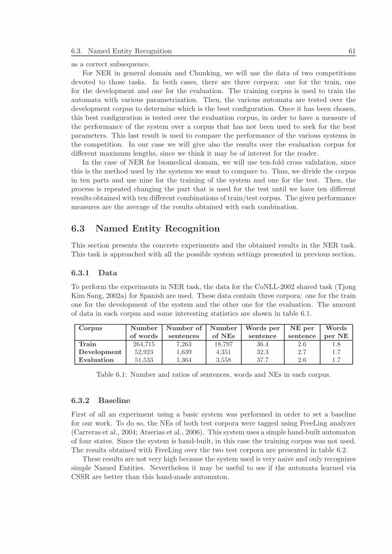
6.3. Named Entity Recognition 61
as a correct subsequence.For NER in general domain and Chunking, we will use the data of two competitions
devoted to those tasks. In both cases, there are three corpora: one for the train, onefor the development and one for the evaluation. The training corpus is used to train theautomata with various parametrization. Then, the various automata are tested over thedevelopment corpus to determine which is the best configuration. Once it has been chosen,this best configuration is tested over the evaluation corpus, in order to have a measure ofthe performance of the system over a corpus that has not been used to seek for the bestparameters. This last result is used to compare the performance of the various systems inthe competition. In our case we will give also the results over the evaluation corpus fordifferent maximum lengths, since we think it may be of interest for the reader.
In the case of NER for biomedical domain, we will use ten-fold cross validation, sincethis is the method used by the systems we want to compare to. Thus, we divide the corpusin ten parts and use nine for the training of the system and one for the test. Then, theprocess is repeated changing the part that is used for the test until we have ten differentresults obtained with ten different combinations of train/test corpus. The given performancemeasures are the average of the results obtained with each combination.
6.3 Named Entity Recognition
This section presents the concrete experiments and the obtained results in the NER task.This task is approached with all the possible system settings presented in previous section.
6.3.1 Data
To perform the experiments in NER task, the data for the CoNLL-2002 shared task (TjongKim Sang, 2002a) for Spanish are used. These data contain three corpora: one for the trainone for the development of the system and the other one for the evaluation. The amountof data in each corpus and some interesting statistics are shown in table 6.1.
Corpus Number Number of Number Words per NE per Words
of words sentences of NEs sentence sentence per NE
Train 264,715 7,263 18,797 36.4 2.6 1.8Development 52,923 1,639 4,351 32.3 2.7 1.7Evaluation 51,533 1,364 3,558 37.7 2.6 1.7
Table 6.1: Number and ratios of sentences, words and NEs in each corpus.
6.3.2 Baseline
First of all an experiment using a basic system was performed in order to set a baselinefor our work. To do so, the NEs of both test corpora were tagged using FreeLing analyzer(Carreras et al., 2004; Atserias et al., 2006). This system uses a simple hand-built automatonof four states. Since the system is hand-built, in this case the training corpus was not used.The results obtained with FreeLing over the two test corpora are presented in table 6.2.
These results are not very high because the system used is very naive and only recognizessimple Named Entities. Nevertheless it may be useful to see if the automata learned viaCSSR are better than this hand-made automaton.

62 Chapter 6. Experiments and Results with CSSR in Annotation Tasks
Precision Recall F1
Development 79.83 88.32 83.86Evaluation 79.14 90.02 84.23
Table 6.2: Obtained results using FreeLing analyzer over the two test corpora.
6.3.3 Alphabet
The alphabet used to build automata using CSSR algorithm to perform Named EntityRecognition was the same used in the example 5.2.1, also used to validate the proposedmethod (section 5.5): GB , GI , GO, SB , SI , SO, MB , MI , MO, aB , aI , aO, wB , wI , wO.
6.3.4 Experiments and Results
Various experiments with the eight different settings presented in section 6.1 and withdifferent values for the parameters were conducted. First of all, we made the experimentsusing χ2 test and using only short suffixes to determine the recurrent states, as it is inthe original CSSR implementation. Nevertheless, we found that this system had a strangebehavior, specially for long lmax (3 or 4) and studying more accurately the error sources,we realized that the problem was due to the fact that the system deleted necessary suffixesbecause they belonged to recurrent states.
To avoid that problem, we changed the way in which the recurrent states are determined,studying the transitions for all suffixes, as it has been explained in section 6.1.4. This led toa better performance of the system. Though the best results are similar, the second systemis much better behaved for long maximum length values and the results depend less on theparameters.
Furthermore, we were interested in testing the use of Jensen-Shannon divergence asan alternative to χ2 hypothesis test. We repeated the experiments using short and longsuffixes to determine the recurrent states. The first approach produced similar results tothose of χ2 test for lmax = 1 or lmax = 2. For longer lmax values, though the systemwas less dependant on the parameters, the obtained results were far behind the best resultsobtained using χ2. Nevertheless this loose in performance was solved when using all suffixesto determine the recurrent states, obtaining a similar performance to the χ2 system thatuses also all suffixes.
In all cases, also the two sink methods, sink-1 and sink-2 were tested. In general, theresults obtained with both methods are similar, specially the best results, but the secondmethod makes the system a little less dependent on the parameters, specially when usingshort suffixes to determine recurrent states.
Next sections present the detailed results for each possible system configuration in-troduced in section 6.1. This is, using χ2 test or Jensen Shannon divergence both withshort and long suffixes when determining the recurrent states. Also the two sink methodspresented in section 6.1.3 are tested in each case.
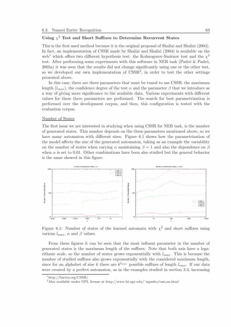
6.3. Named Entity Recognition 63
Using χ2 Test and Short Suffixes to Determine Recurrent States
This is the first used method because it is the original proposal of Shalizi and Shalizi (2004).In fact, an implementation of CSSR made by Shalizi and Shalizi (2004) is available on theweb1 which offers two different hypothesis test: the Kolmogorov-Smirnov test and the χ2
test. After performing some experiments with this software in NER task (Padro & Padro,2005a) it was seen that the results did not change significantly using one or the other test,so we developed our own implementation of CSSR2, in order to test the other settingspresented above.
In this case, there are three parameters that must be tuned to use CSSR: the maximumlength (lmax), the confidence degree of the test α and the parameter β that we introduce asa way of giving more significance to the available data. Various experiments with differentvalues for these three parameters are performed. The search for best parametrization isperformed over the development corpus, and then, this configuration is tested with theevaluation corpus.
Number of States
The first issue we are interested in studying when using CSSR for NER task, is the numberof generated states. This number depends on the three parameters mentioned above, so wehave many automaton with different sizes. Figure 6.1 shows how the parametrization ofthe model affects the size of the generated automaton, taking as an example the variabilityon the number of states when varying α maintaining β = 1 and also the dependence on βwhen α is set to 0.01. Other combinations have been also studied but the general behavioris the same showed in this figure.
Figure 6.1: Number of states of the learned automata with χ2 and short suffixes usingvarious lmax, α and β values.
From these figures it can be seen that the most influent parameter in the number ofgenerated states is the maximum length of the suffixes. Note that both axis have a loga-rithmic scale, so the number of states grows exponentially with lmax. This is because thenumber of studied suffixes also grows exponentially with the considered maximum length,since for an alphabet of size k there are klmax possible suffixes of length lmax. If our datawere created by a perfect automaton, as in the examples studied in section 3.3, increasing
1http://bactra.org/CSSR/2Also available under GPL license at http://www.lsi.upc.edu/˜mpadro/cssr en.html
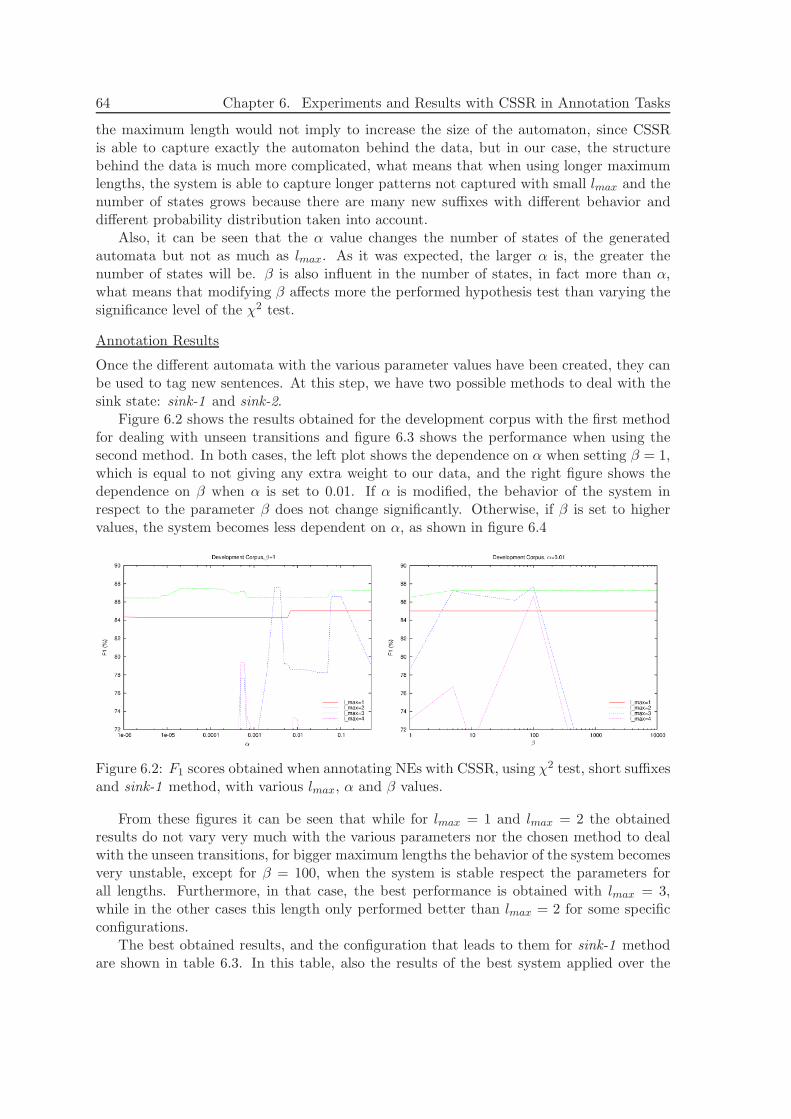
64 Chapter 6. Experiments and Results with CSSR in Annotation Tasks
the maximum length would not imply to increase the size of the automaton, since CSSRis able to capture exactly the automaton behind the data, but in our case, the structurebehind the data is much more complicated, what means that when using longer maximumlengths, the system is able to capture longer patterns not captured with small lmax and thenumber of states grows because there are many new suffixes with different behavior anddifferent probability distribution taken into account.
Also, it can be seen that the α value changes the number of states of the generatedautomata but not as much as lmax. As it was expected, the larger α is, the greater thenumber of states will be. β is also influent in the number of states, in fact more than α,what means that modifying β affects more the performed hypothesis test than varying thesignificance level of the χ2 test.
Annotation Results
Once the different automata with the various parameter values have been created, they canbe used to tag new sentences. At this step, we have two possible methods to deal with thesink state: sink-1 and sink-2.
Figure 6.2 shows the results obtained for the development corpus with the first methodfor dealing with unseen transitions and figure 6.3 shows the performance when using thesecond method. In both cases, the left plot shows the dependence on α when setting β = 1,which is equal to not giving any extra weight to our data, and the right figure shows thedependence on β when α is set to 0.01. If α is modified, the behavior of the system inrespect to the parameter β does not change significantly. Otherwise, if β is set to highervalues, the system becomes less dependent on α, as shown in figure 6.4
Figure 6.2: F1 scores obtained when annotating NEs with CSSR, using χ2 test, short suffixesand sink-1 method, with various lmax, α and β values.
From these figures it can be seen that while for lmax = 1 and lmax = 2 the obtainedresults do not vary very much with the various parameters nor the chosen method to dealwith the unseen transitions, for bigger maximum lengths the behavior of the system becomesvery unstable, except for β = 100, when the system is stable respect the parameters forall lengths. Furthermore, in that case, the best performance is obtained with lmax = 3,while in the other cases this length only performed better than lmax = 2 for some specificconfigurations.
The best obtained results, and the configuration that leads to them for sink-1 methodare shown in table 6.3. In this table, also the results of the best system applied over the
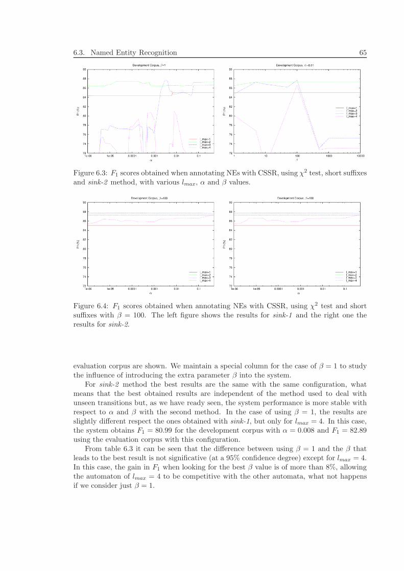
6.3. Named Entity Recognition 65
Figure 6.3: F1 scores obtained when annotating NEs with CSSR, using χ2 test, short suffixesand sink-2 method, with various lmax, α and β values.
Figure 6.4: F1 scores obtained when annotating NEs with CSSR, using χ2 test and shortsuffixes with β = 100. The left figure shows the results for sink-1 and the right one theresults for sink-2.
evaluation corpus are shown. We maintain a special column for the case of β = 1 to studythe influence of introducing the extra parameter β into the system.
For sink-2 method the best results are the same with the same configuration, whatmeans that the best obtained results are independent of the method used to deal withunseen transitions but, as we have ready seen, the system performance is more stable withrespect to α and β with the second method. In the case of using β = 1, the results areslightly different respect the ones obtained with sink-1, but only for lmax = 4. In this case,the system obtains F1 = 80.99 for the development corpus with α = 0.008 and F1 = 82.89using the evaluation corpus with this configuration.
From table 6.3 it can be seen that the difference between using β = 1 and the β thatleads to the best result is not significative (at a 95% confidence degree) except for lmax = 4.In this case, the gain in F1 when looking for the best β value is of more than 8%, allowingthe automaton of lmax = 4 to be competitive with the other automata, what not happensif we consider just β = 1.
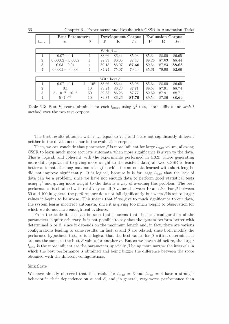
66 Chapter 6. Experiments and Results with CSSR in Annotation Tasks
Best Parameters Development Corpus Evaluation Corpus
lmax α β P R F1 P R F1
With β = 11 0.07 – 0.1 1 83.66 86.44 85.03 85.34 88.00 86.652 0.00002 – 0.0002 1 88.99 86.05 87.45 89.26 87.63 88.443 0.03 – 0.04 1 89.18 86.07 87.60 89.54 87.83 88.68
4 0.0005 – 0.0006 1 84.24 75.07 79.40 85.61 79.90 82.66
With best β1 0.07 – 0.1 1 – 106 83.66 86.44 85.03 85.34 88.00 86.652 0.1 10 89.24 86.23 87.71 89.58 87.91 88.743 5 · 10−6– 10−5 50 89.33 86.26 87.77 89.52 87.91 88.714 5 · 10−6 10 89.37 86.26 87.79 89.54 87.86 88.69
Table 6.3: Best F1 scores obtained for each lmax, using χ2 test, short suffixes and sink-1method over the two test corpora.
The best results obtained with lmax equal to 2, 3 and 4 are not significantly differentneither in the development nor in the evaluation corpus.
Then, we can conclude that parameter β is more influent for large lmax values, allowingCSSR to learn much more accurate automata when more significance is given to the data.This is logical, and coherent with the experiments performed in 4.3.2, where generatingmore data (equivalent to giving more weight to the existent data) allowed CSSR to learnbetter automata for long maximum lengths while the automata learned with short lengthsdid not improve significantly. It is logical, because it is for large lmax that the lack ofdata can be a problem, since we have not enough data to perform good statistical testsusing χ2 and giving more weight to the data is a way of avoiding this problem. The bestperformance is obtained with relatively small β values, between 10 and 50. For β between50 and 100 in general the performance does not fall significantly but when β is set to largervalues it begins to be worse. This means that if we give to much significance to our data,the system learns incorrect automata, since it is giving too much weight to observation forwhich we do not have enough real evidence.
From the table it also can be seen that it seems that the best configuration of theparameters is quite arbitrary, it is not possible to say that the system perform better withdetermined α or β, since it depends on the maximum length and, in fact, there are variousconfigurations leading to same results. In fact, α and β are related, since both modify theperformed hypothesis test, so it is logical that the best values for β with a determined αare not the same as the best β values for another α. But as we have said before, the largerlmax is the more influent are the parameters, specially β being more narrow the intervals inwhich the best performance is obtained and being bigger the difference between the scoreobtained with the different configurations.
Sink State
We have already observed that the results for lmax = 3 and lmax = 4 have a strangerbehavior in their dependence on α and β, and, in general, very worse performance than
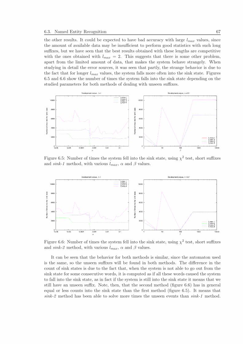
6.3. Named Entity Recognition 67
the other results. It could be expected to have bad accuracy with large lmax values, sincethe amount of available data may be insufficient to perform good statistics with such longsuffixes, but we have seen that the best results obtained with these lengths are competitivewith the ones obtained with lmax = 2. This suggests that there is some other problem,apart from the limited amount of data, that makes the system behave strangely. Whenstudying in detail the error sources, it was seen that partly, the strange behavior is due tothe fact that for longer lmax values, the system falls more often into the sink state. Figures6.5 and 6.6 show the number of times the system falls into the sink state depending on thestudied parameters for both methods of dealing with unseen suffixes.
Figure 6.5: Number of times the system fell into the sink state, using χ2 test, short suffixesand sink-1 method, with various lmax, α and β values.
Figure 6.6: Number of times the system fell into the sink state, using χ2 test, short suffixesand sink-2 method, with various lmax, α and β values.
It can be seen that the behavior for both methods is similar, since the automaton usedis the same, so the unseen suffixes will be found in both methods. The difference in thecount of sink states is due to the fact that, when the system is not able to go out from thesink state for some consecutive words, it is computed as if all these words caused the systemto fall into the sink state, as in fact if the system is still into the sink state it means that westill have an unseen suffix. Note, then, that the second method (figure 6.6) has in generalequal or less counts into the sink state than the first method (figure 6.5). It means thatsink-2 method has been able to solve more times the unseen events than sink-1 method.
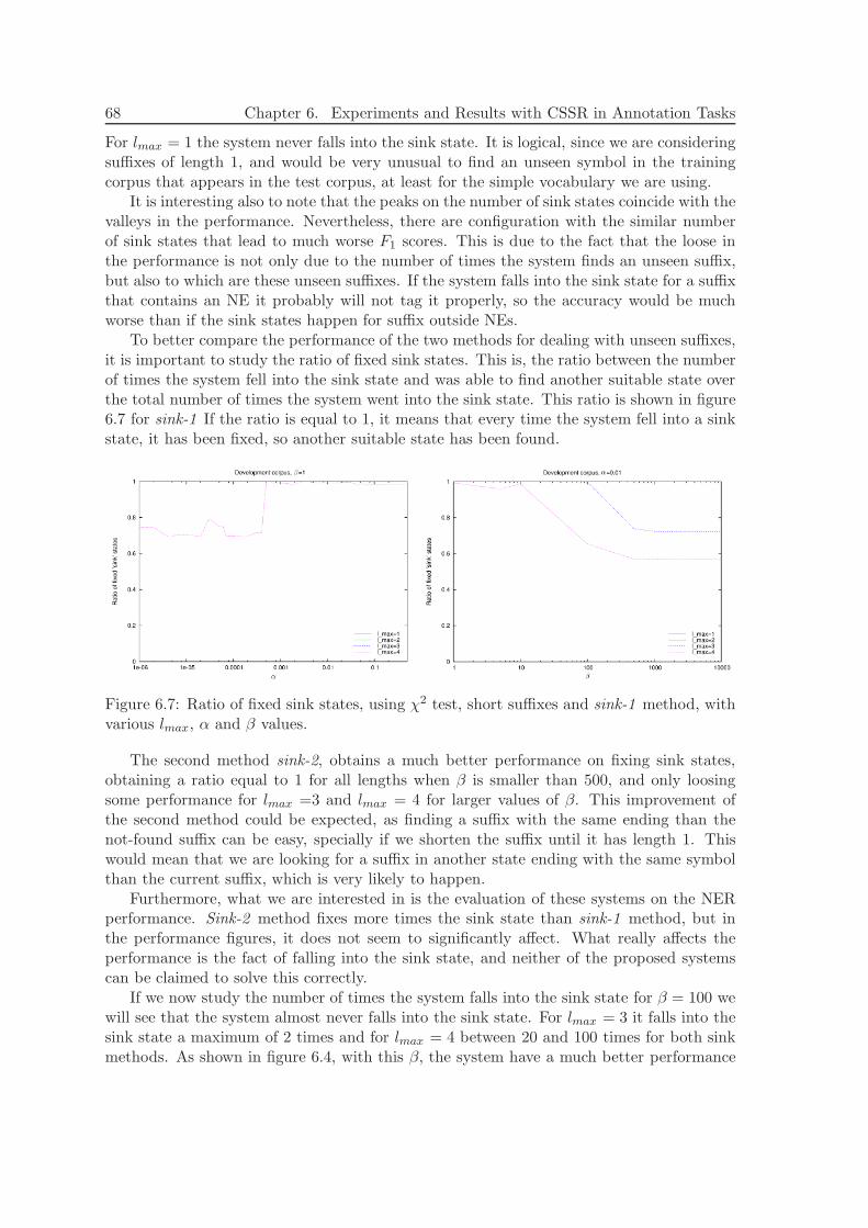
68 Chapter 6. Experiments and Results with CSSR in Annotation Tasks
For lmax = 1 the system never falls into the sink state. It is logical, since we are consideringsuffixes of length 1, and would be very unusual to find an unseen symbol in the trainingcorpus that appears in the test corpus, at least for the simple vocabulary we are using.
It is interesting also to note that the peaks on the number of sink states coincide with thevalleys in the performance. Nevertheless, there are configuration with the similar numberof sink states that lead to much worse F1 scores. This is due to the fact that the loose inthe performance is not only due to the number of times the system finds an unseen suffix,but also to which are these unseen suffixes. If the system falls into the sink state for a suffixthat contains an NE it probably will not tag it properly, so the accuracy would be muchworse than if the sink states happen for suffix outside NEs.
To better compare the performance of the two methods for dealing with unseen suffixes,it is important to study the ratio of fixed sink states. This is, the ratio between the numberof times the system fell into the sink state and was able to find another suitable state overthe total number of times the system went into the sink state. This ratio is shown in figure6.7 for sink-1 If the ratio is equal to 1, it means that every time the system fell into a sinkstate, it has been fixed, so another suitable state has been found.
Figure 6.7: Ratio of fixed sink states, using χ2 test, short suffixes and sink-1 method, withvarious lmax, α and β values.
The second method sink-2, obtains a much better performance on fixing sink states,obtaining a ratio equal to 1 for all lengths when β is smaller than 500, and only loosingsome performance for lmax =3 and lmax = 4 for larger values of β. This improvement ofthe second method could be expected, as finding a suffix with the same ending than thenot-found suffix can be easy, specially if we shorten the suffix until it has length 1. Thiswould mean that we are looking for a suffix in another state ending with the same symbolthan the current suffix, which is very likely to happen.
Furthermore, what we are interested in is the evaluation of these systems on the NERperformance. Sink-2 method fixes more times the sink state than sink-1 method, but inthe performance figures, it does not seem to significantly affect. What really affects theperformance is the fact of falling into the sink state, and neither of the proposed systemscan be claimed to solve this correctly.
If we now study the number of times the system falls into the sink state for β = 100 wewill see that the system almost never falls into the sink state. For lmax = 3 it falls into thesink state a maximum of 2 times and for lmax = 4 between 20 and 100 times for both sinkmethods. As shown in figure 6.4, with this β, the system have a much better performance
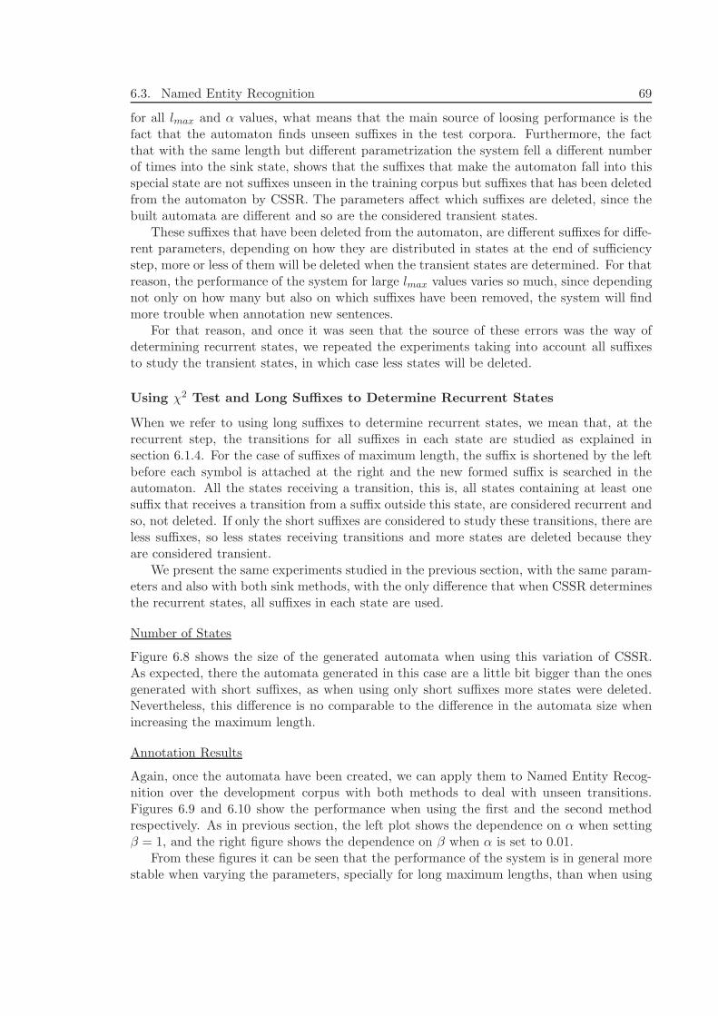
6.3. Named Entity Recognition 69
for all lmax and α values, what means that the main source of loosing performance is thefact that the automaton finds unseen suffixes in the test corpora. Furthermore, the factthat with the same length but different parametrization the system fell a different numberof times into the sink state, shows that the suffixes that make the automaton fall into thisspecial state are not suffixes unseen in the training corpus but suffixes that has been deletedfrom the automaton by CSSR. The parameters affect which suffixes are deleted, since thebuilt automata are different and so are the considered transient states.
These suffixes that have been deleted from the automaton, are different suffixes for diffe-rent parameters, depending on how they are distributed in states at the end of sufficiencystep, more or less of them will be deleted when the transient states are determined. For thatreason, the performance of the system for large lmax values varies so much, since dependingnot only on how many but also on which suffixes have been removed, the system will findmore trouble when annotation new sentences.
For that reason, and once it was seen that the source of these errors was the way ofdetermining recurrent states, we repeated the experiments taking into account all suffixesto study the transient states, in which case less states will be deleted.
Using χ2 Test and Long Suffixes to Determine Recurrent States
When we refer to using long suffixes to determine recurrent states, we mean that, at therecurrent step, the transitions for all suffixes in each state are studied as explained insection 6.1.4. For the case of suffixes of maximum length, the suffix is shortened by the leftbefore each symbol is attached at the right and the new formed suffix is searched in theautomaton. All the states receiving a transition, this is, all states containing at least onesuffix that receives a transition from a suffix outside this state, are considered recurrent andso, not deleted. If only the short suffixes are considered to study these transitions, there areless suffixes, so less states receiving transitions and more states are deleted because theyare considered transient.
We present the same experiments studied in the previous section, with the same param-eters and also with both sink methods, with the only difference that when CSSR determinesthe recurrent states, all suffixes in each state are used.
Number of States
Figure 6.8 shows the size of the generated automata when using this variation of CSSR.As expected, there the automata generated in this case are a little bit bigger than the onesgenerated with short suffixes, as when using only short suffixes more states were deleted.Nevertheless, this difference is no comparable to the difference in the automata size whenincreasing the maximum length.
Annotation Results
Again, once the automata have been created, we can apply them to Named Entity Recog-nition over the development corpus with both methods to deal with unseen transitions.Figures 6.9 and 6.10 show the performance when using the first and the second methodrespectively. As in previous section, the left plot shows the dependence on α when settingβ = 1, and the right figure shows the dependence on β when α is set to 0.01.
From these figures it can be seen that the performance of the system is in general morestable when varying the parameters, specially for long maximum lengths, than when using
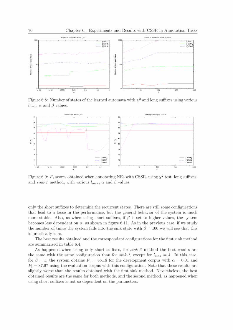
70 Chapter 6. Experiments and Results with CSSR in Annotation Tasks
Figure 6.8: Number of states of the learned automata with χ2 and long suffixes using variouslmax, α and β values.
Figure 6.9: F1 scores obtained when annotating NEs with CSSR, using χ2 test, long suffixes,and sink-1 method, with various lmax, α and β values.
only the short suffixes to determine the recurrent states. There are still some configurationsthat lead to a loose in the performance, but the general behavior of the system is muchmore stable. Also, as when using short suffixes, if β is set to higher values, the systembecomes less dependent on α, as shown in figure 6.11. As in the previous case, if we studythe number of times the system falls into the sink state with β = 100 we will see that thisis practically zero.
The best results obtained and the correspondant configurations for the first sink methodare summarized in table 6.4.
As happened when using only short suffixes, for sink-2 method the best results arethe same with the same configuration than for sink-1, except for lmax = 4. In this case,for β = 1, the system obtains F1 = 86.18 for the development corpus with α = 0.01 andF1 = 87.97 using the evaluation corpus with this configuration. Note that these results areslightly worse than the results obtained with the first sink method. Nevertheless, the bestobtained results are the same for both methods, and the second method, as happened whenusing short suffixes is not so dependent on the parameters.
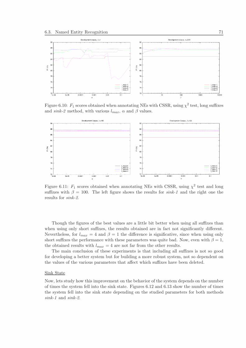
6.3. Named Entity Recognition 71
Figure 6.10: F1 scores obtained when annotating NEs with CSSR, using χ2 test, long suffixesand sink-2 method, with various lmax, α and β values.
Figure 6.11: F1 scores obtained when annotating NEs with CSSR, using χ2 test and longsuffixes with β = 100. The left figure shows the results for sink-1 and the right one theresults for sink-2.
Though the figures of the best values are a little bit better when using all suffixes thanwhen using only short suffixes, the results obtained are in fact not significantly different.Nevertheless, for lmax = 4 and β = 1 the difference is significative, since when using onlyshort suffixes the performance with these parameters was quite bad. Now, even with β = 1,the obtained results with lmax = 4 are not far from the other results.
The main conclusion of these experiments is that including all suffixes is not so goodfor developing a better system but for building a more robust system, not so dependent onthe values of the various parameters that affect which suffixes have been deleted.
Sink State
Now, lets study how this improvement on the behavior of the system depends on the numberof times the system fell into the sink state. Figures 6.12 and 6.13 show the number of timesthe system fell into the sink state depending on the studied parameters for both methodssink-1 and sink-2.
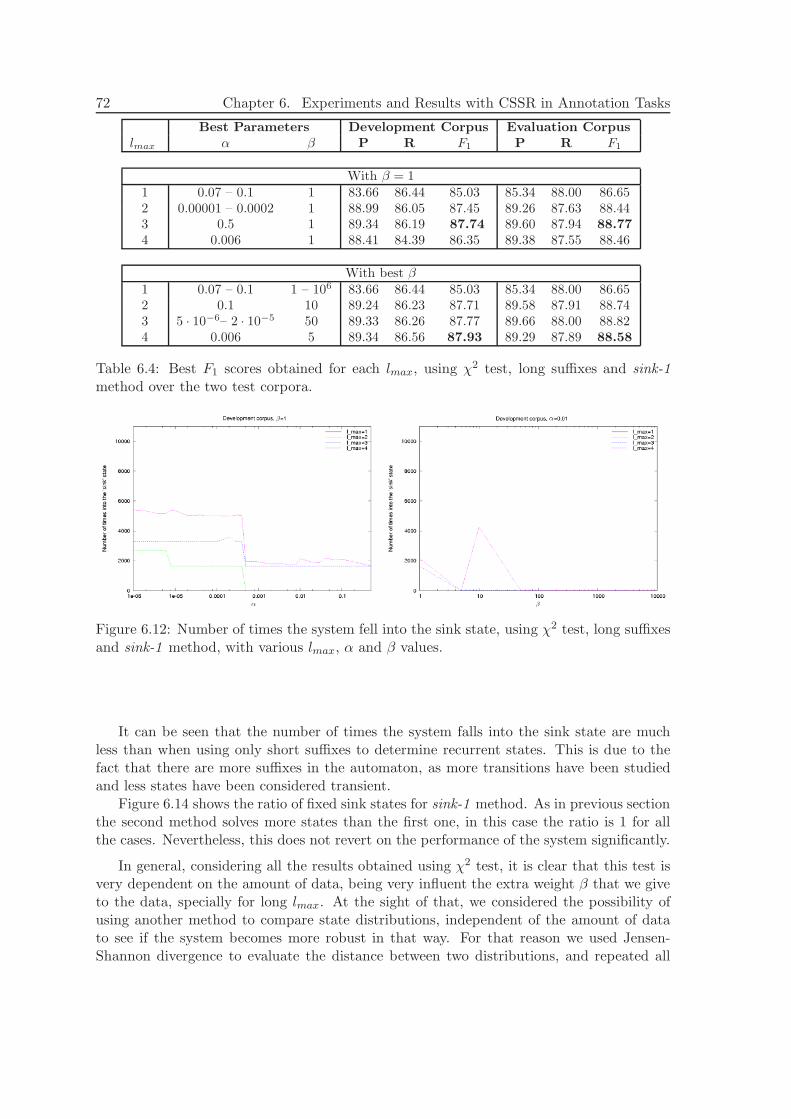
72 Chapter 6. Experiments and Results with CSSR in Annotation Tasks
Best Parameters Development Corpus Evaluation Corpus
lmax α β P R F1 P R F1
With β = 11 0.07 – 0.1 1 83.66 86.44 85.03 85.34 88.00 86.652 0.00001 – 0.0002 1 88.99 86.05 87.45 89.26 87.63 88.443 0.5 1 89.34 86.19 87.74 89.60 87.94 88.77
4 0.006 1 88.41 84.39 86.35 89.38 87.55 88.46
With best β1 0.07 – 0.1 1 – 106 83.66 86.44 85.03 85.34 88.00 86.652 0.1 10 89.24 86.23 87.71 89.58 87.91 88.743 5 · 10−6– 2 · 10−5 50 89.33 86.26 87.77 89.66 88.00 88.824 0.006 5 89.34 86.56 87.93 89.29 87.89 88.58
Table 6.4: Best F1 scores obtained for each lmax, using χ2 test, long suffixes and sink-1method over the two test corpora.
Figure 6.12: Number of times the system fell into the sink state, using χ2 test, long suffixesand sink-1 method, with various lmax, α and β values.
It can be seen that the number of times the system falls into the sink state are muchless than when using only short suffixes to determine recurrent states. This is due to thefact that there are more suffixes in the automaton, as more transitions have been studiedand less states have been considered transient.
Figure 6.14 shows the ratio of fixed sink states for sink-1 method. As in previous sectionthe second method solves more states than the first one, in this case the ratio is 1 for allthe cases. Nevertheless, this does not revert on the performance of the system significantly.
In general, considering all the results obtained using χ2 test, it is clear that this test isvery dependent on the amount of data, being very influent the extra weight β that we giveto the data, specially for long lmax. At the sight of that, we considered the possibility ofusing another method to compare state distributions, independent of the amount of datato see if the system becomes more robust in that way. For that reason we used Jensen-Shannon divergence to evaluate the distance between two distributions, and repeated all
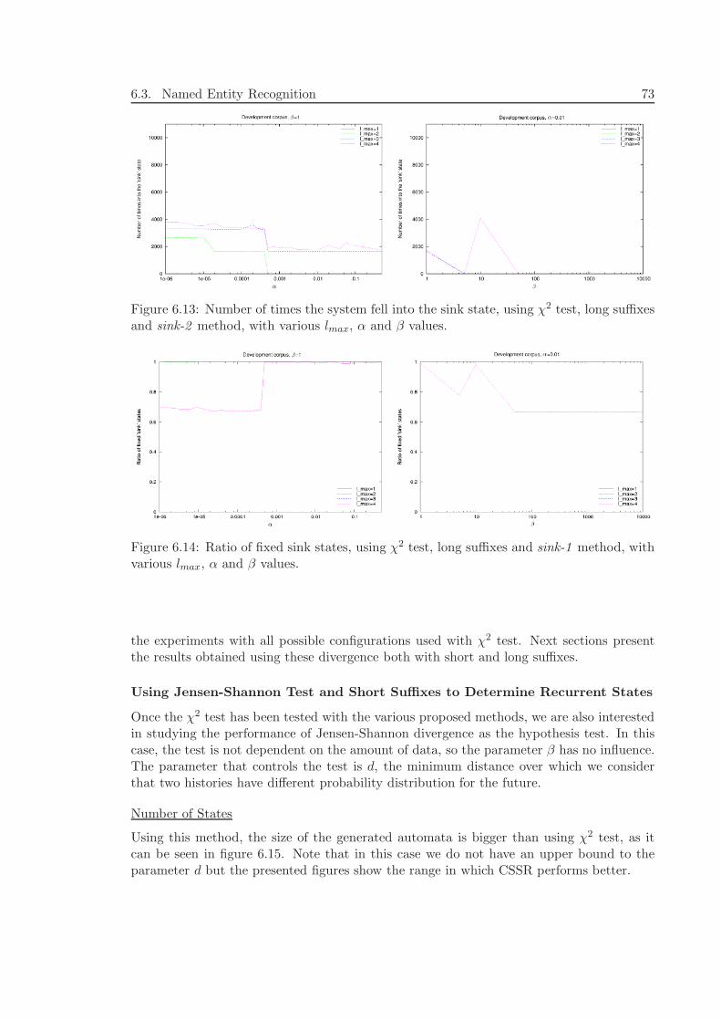
6.3. Named Entity Recognition 73
Figure 6.13: Number of times the system fell into the sink state, using χ2 test, long suffixesand sink-2 method, with various lmax, α and β values.
Figure 6.14: Ratio of fixed sink states, using χ2 test, long suffixes and sink-1 method, withvarious lmax, α and β values.
the experiments with all possible configurations used with χ2 test. Next sections presentthe results obtained using these divergence both with short and long suffixes.
Using Jensen-Shannon Test and Short Suffixes to Determine Recurrent States
Once the χ2 test has been tested with the various proposed methods, we are also interestedin studying the performance of Jensen-Shannon divergence as the hypothesis test. In thiscase, the test is not dependent on the amount of data, so the parameter β has no influence.The parameter that controls the test is d, the minimum distance over which we considerthat two histories have different probability distribution for the future.
Number of States
Using this method, the size of the generated automata is bigger than using χ2 test, as itcan be seen in figure 6.15. Note that in this case we do not have an upper bound to theparameter d but the presented figures show the range in which CSSR performs better.
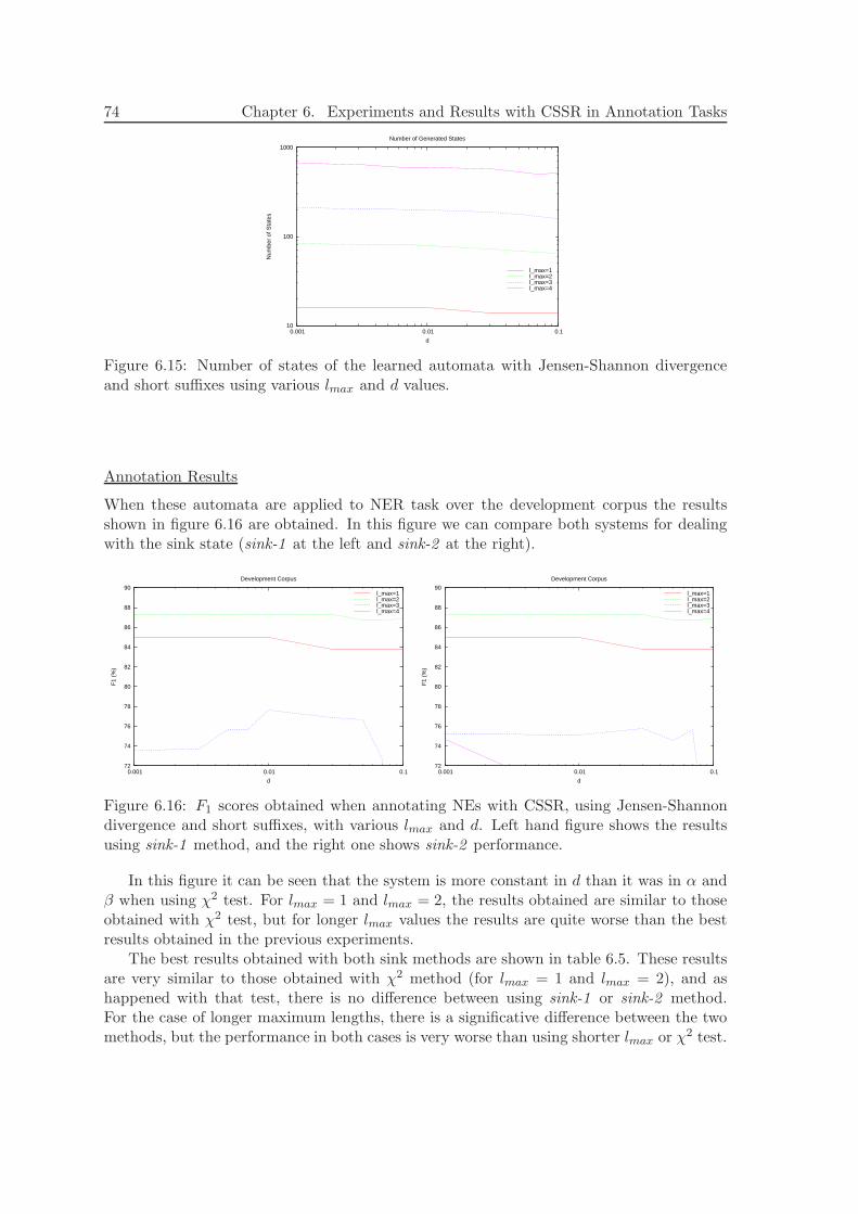
74 Chapter 6. Experiments and Results with CSSR in Annotation Tasks
10
100
1000
0.001 0.01 0.1
Num
ber
of S
tate
s
d
Number of Generated States
l_max=1l_max=2l_max=3l_max=4
Figure 6.15: Number of states of the learned automata with Jensen-Shannon divergenceand short suffixes using various lmax and d values.
Annotation Results
When these automata are applied to NER task over the development corpus the resultsshown in figure 6.16 are obtained. In this figure we can compare both systems for dealingwith the sink state (sink-1 at the left and sink-2 at the right).
72
74
76
78
80
82
84
86
88
90
0.001 0.01 0.1
F1
(%)
d
Development Corpus
l_max=1l_max=2l_max=3l_max=4
72
74
76
78
80
82
84
86
88
90
0.001 0.01 0.1
F1
(%)
d
Development Corpus
l_max=1l_max=2l_max=3l_max=4
Figure 6.16: F1 scores obtained when annotating NEs with CSSR, using Jensen-Shannondivergence and short suffixes, with various lmax and d. Left hand figure shows the resultsusing sink-1 method, and the right one shows sink-2 performance.
In this figure it can be seen that the system is more constant in d than it was in α andβ when using χ2 test. For lmax = 1 and lmax = 2, the results obtained are similar to thoseobtained with χ2 test, but for longer lmax values the results are quite worse than the bestresults obtained in the previous experiments.
The best results obtained with both sink methods are shown in table 6.5. These resultsare very similar to those obtained with χ2 method (for lmax = 1 and lmax = 2), and ashappened with that test, there is no difference between using sink-1 or sink-2 method.For the case of longer maximum lengths, there is a significative difference between the twomethods, but the performance in both cases is very worse than using shorter lmax or χ2 test.
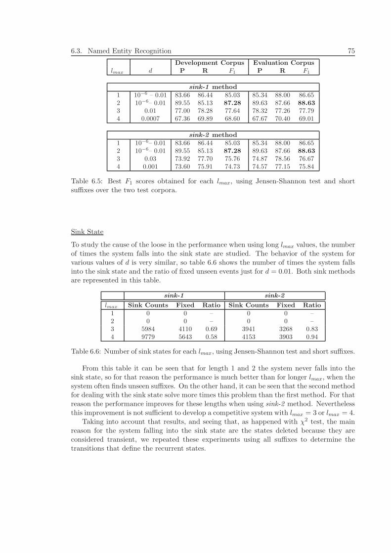
6.3. Named Entity Recognition 75
Development Corpus Evaluation Corpus
lmax d P R F1 P R F1
sink-1 method
1 10−6 – 0.01 83.66 86.44 85.03 85.34 88.00 86.652 10−6– 0.01 89.55 85.13 87.28 89.63 87.66 88.63
3 0.01 77.00 78.28 77.64 78.32 77.26 77.794 0.0007 67.36 69.89 68.60 67.67 70.40 69.01
sink-2 method
1 10−6– 0.01 83.66 86.44 85.03 85.34 88.00 86.652 10−6– 0.01 89.55 85.13 87.28 89.63 87.66 88.63
3 0.03 73.92 77.70 75.76 74.87 78.56 76.674 0.001 73.60 75.91 74.73 74.57 77.15 75.84
Table 6.5: Best F1 scores obtained for each lmax, using Jensen-Shannon test and shortsuffixes over the two test corpora.
Sink State
To study the cause of the loose in the performance when using long lmax values, the numberof times the system falls into the sink state are studied. The behavior of the system forvarious values of d is very similar, so table 6.6 shows the number of times the system fallsinto the sink state and the ratio of fixed unseen events just for d = 0.01. Both sink methodsare represented in this table.
sink-1 sink-2
lmax Sink Counts Fixed Ratio Sink Counts Fixed Ratio
1 0 0 – 0 0 –2 0 0 – 0 0 –3 5984 4110 0.69 3941 3268 0.834 9779 5643 0.58 4153 3903 0.94
Table 6.6: Number of sink states for each lmax, using Jensen-Shannon test and short suffixes.
From this table it can be seen that for length 1 and 2 the system never falls into thesink state, so for that reason the performance is much better than for longer lmax, when thesystem often finds unseen suffixes. On the other hand, it can be seen that the second methodfor dealing with the sink state solve more times this problem than the first method. For thatreason the performance improves for these lengths when using sink-2 method. Neverthelessthis improvement is not sufficient to develop a competitive system with lmax = 3 or lmax = 4.
Taking into account that results, and seeing that, as happened with χ2 test, the mainreason for the system falling into the sink state are the states deleted because they areconsidered transient, we repeated these experiments using all suffixes to determine thetransitions that define the recurrent states.
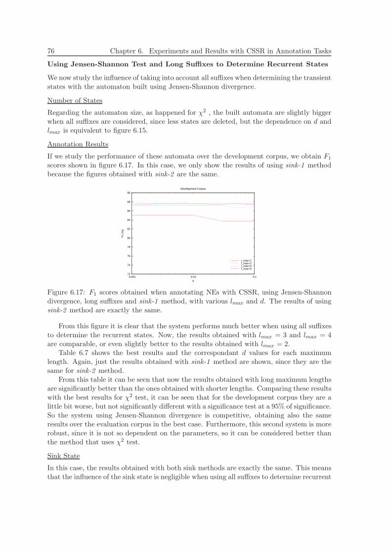
76 Chapter 6. Experiments and Results with CSSR in Annotation Tasks
Using Jensen-Shannon Test and Long Suffixes to Determine Recurrent States
We now study the influence of taking into account all suffixes when determining the transientstates with the automaton built using Jensen-Shannon divergence.
Number of States
Regarding the automaton size, as happened for χ2 , the built automata are slightly biggerwhen all suffixes are considered, since less states are deleted, but the dependence on d andlmax is equivalent to figure 6.15.
Annotation Results
If we study the performance of these automata over the development corpus, we obtain F1
scores shown in figure 6.17. In this case, we only show the results of using sink-1 methodbecause the figures obtained with sink-2 are the same.
72
74
76
78
80
82
84
86
88
90
0.001 0.01 0.1
F1
(%)
d
Development Corpus
l_max=1l_max=2l_max=3l_max=4
Figure 6.17: F1 scores obtained when annotating NEs with CSSR, using Jensen-Shannondivergence, long suffixes and sink-1 method, with various lmax and d. The results of usingsink-2 method are exactly the same.
From this figure it is clear that the system performs much better when using all suffixesto determine the recurrent states. Now, the results obtained with lmax = 3 and lmax = 4are comparable, or even slightly better to the results obtained with lmax = 2.
Table 6.7 shows the best results and the correspondant d values for each maximumlength. Again, just the results obtained with sink-1 method are shown, since they are thesame for sink-2 method.
From this table it can be seen that now the results obtained with long maximum lengthsare significantly better than the ones obtained with shorter lengths. Comparing these resultswith the best results for χ2 test, it can be seen that for the development corpus they are alittle bit worse, but not significantly different with a significance test at a 95% of significance.So the system using Jensen-Shannon divergence is competitive, obtaining also the sameresults over the evaluation corpus in the best case. Furthermore, this second system is morerobust, since it is not so dependent on the parameters, so it can be considered better thanthe method that uses χ2 test.
Sink State
In this case, the results obtained with both sink methods are exactly the same. This meansthat the influence of the sink state is negligible when using all suffixes to determine recurrent
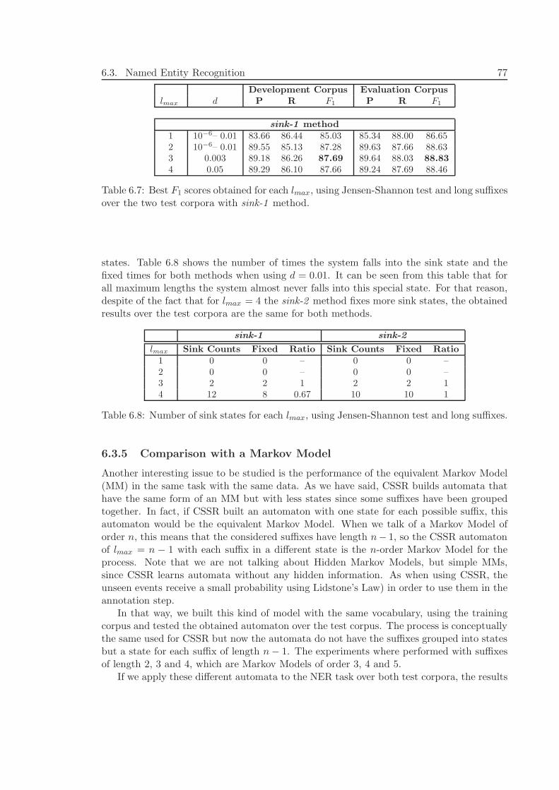
6.3. Named Entity Recognition 77
Development Corpus Evaluation Corpus
lmax d P R F1 P R F1
sink-1 method
1 10−6– 0.01 83.66 86.44 85.03 85.34 88.00 86.652 10−6– 0.01 89.55 85.13 87.28 89.63 87.66 88.633 0.003 89.18 86.26 87.69 89.64 88.03 88.83
4 0.05 89.29 86.10 87.66 89.24 87.69 88.46
Table 6.7: Best F1 scores obtained for each lmax, using Jensen-Shannon test and long suffixesover the two test corpora with sink-1 method.
states. Table 6.8 shows the number of times the system falls into the sink state and thefixed times for both methods when using d = 0.01. It can be seen from this table that forall maximum lengths the system almost never falls into this special state. For that reason,despite of the fact that for lmax = 4 the sink-2 method fixes more sink states, the obtainedresults over the test corpora are the same for both methods.
sink-1 sink-2
lmax Sink Counts Fixed Ratio Sink Counts Fixed Ratio
1 0 0 – 0 0 –2 0 0 – 0 0 –3 2 2 1 2 2 14 12 8 0.67 10 10 1
Table 6.8: Number of sink states for each lmax, using Jensen-Shannon test and long suffixes.
6.3.5 Comparison with a Markov Model
Another interesting issue to be studied is the performance of the equivalent Markov Model(MM) in the same task with the same data. As we have said, CSSR builds automata thathave the same form of an MM but with less states since some suffixes have been groupedtogether. In fact, if CSSR built an automaton with one state for each possible suffix, thisautomaton would be the equivalent Markov Model. When we talk of a Markov Model oforder n, this means that the considered suffixes have length n− 1, so the CSSR automatonof lmax = n − 1 with each suffix in a different state is the n-order Markov Model for theprocess. Note that we are not talking about Hidden Markov Models, but simple MMs,since CSSR learns automata without any hidden information. As when using CSSR, theunseen events receive a small probability using Lidstone’s Law) in order to use them in theannotation step.
In that way, we built this kind of model with the same vocabulary, using the trainingcorpus and tested the obtained automaton over the test corpus. The process is conceptuallythe same used for CSSR but now the automata do not have the suffixes grouped into statesbut a state for each suffix of length n − 1. The experiments where performed with suffixesof length 2, 3 and 4, which are Markov Models of order 3, 4 and 5.
If we apply these different automata to the NER task over both test corpora, the results
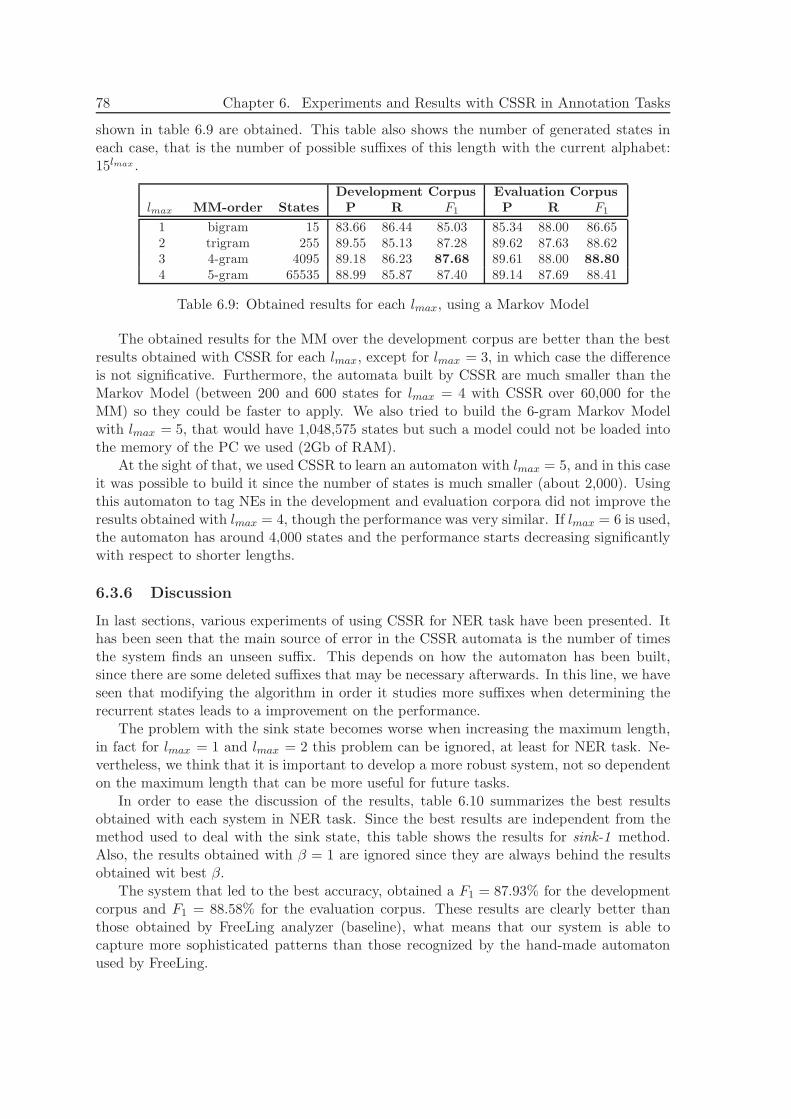
78 Chapter 6. Experiments and Results with CSSR in Annotation Tasks
shown in table 6.9 are obtained. This table also shows the number of generated states ineach case, that is the number of possible suffixes of this length with the current alphabet:15lmax .
Development Corpus Evaluation Corpus
lmax MM-order States P R F1 P R F1
1 bigram 15 83.66 86.44 85.03 85.34 88.00 86.652 trigram 255 89.55 85.13 87.28 89.62 87.63 88.623 4-gram 4095 89.18 86.23 87.68 89.61 88.00 88.80
4 5-gram 65535 88.99 85.87 87.40 89.14 87.69 88.41
Table 6.9: Obtained results for each lmax, using a Markov Model
The obtained results for the MM over the development corpus are better than the bestresults obtained with CSSR for each lmax, except for lmax = 3, in which case the differenceis not significative. Furthermore, the automata built by CSSR are much smaller than theMarkov Model (between 200 and 600 states for lmax = 4 with CSSR over 60,000 for theMM) so they could be faster to apply. We also tried to build the 6-gram Markov Modelwith lmax = 5, that would have 1,048,575 states but such a model could not be loaded intothe memory of the PC we used (2Gb of RAM).
At the sight of that, we used CSSR to learn an automaton with lmax = 5, and in this caseit was possible to build it since the number of states is much smaller (about 2,000). Usingthis automaton to tag NEs in the development and evaluation corpora did not improve theresults obtained with lmax = 4, though the performance was very similar. If lmax = 6 is used,the automaton has around 4,000 states and the performance starts decreasing significantlywith respect to shorter lengths.
6.3.6 Discussion
In last sections, various experiments of using CSSR for NER task have been presented. Ithas been seen that the main source of error in the CSSR automata is the number of timesthe system finds an unseen suffix. This depends on how the automaton has been built,since there are some deleted suffixes that may be necessary afterwards. In this line, we haveseen that modifying the algorithm in order it studies more suffixes when determining therecurrent states leads to a improvement on the performance.
The problem with the sink state becomes worse when increasing the maximum length,in fact for lmax = 1 and lmax = 2 this problem can be ignored, at least for NER task. Ne-vertheless, we think that it is important to develop a more robust system, not so dependenton the maximum length that can be more useful for future tasks.
In order to ease the discussion of the results, table 6.10 summarizes the best resultsobtained with each system in NER task. Since the best results are independent from themethod used to deal with the sink state, this table shows the results for sink-1 method.Also, the results obtained with β = 1 are ignored since they are always behind the resultsobtained wit best β.
The system that led to the best accuracy, obtained a F1 = 87.93% for the developmentcorpus and F1 = 88.58% for the evaluation corpus. These results are clearly better thanthose obtained by FreeLing analyzer (baseline), what means that our system is able tocapture more sophisticated patterns than those recognized by the hand-made automatonused by FreeLing.
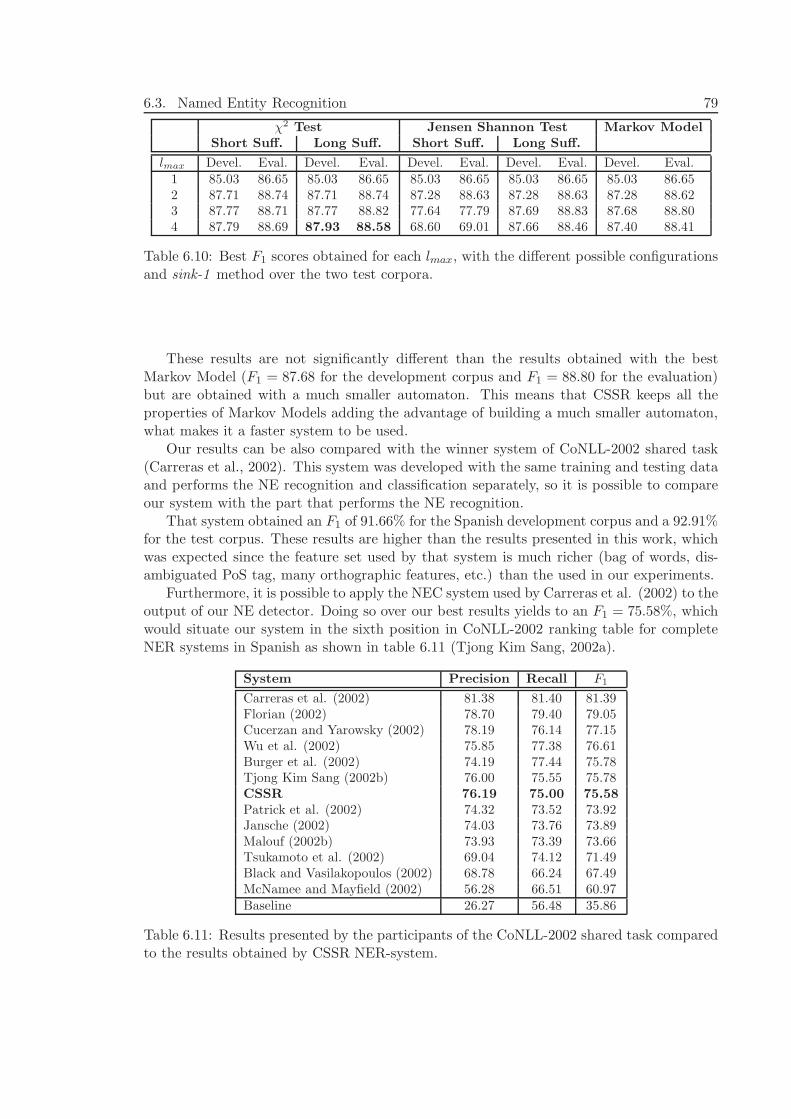
6.3. Named Entity Recognition 79
χ2 Test Jensen Shannon Test Markov Model
Short Suff. Long Suff. Short Suff. Long Suff.
lmax Devel. Eval. Devel. Eval. Devel. Eval. Devel. Eval. Devel. Eval.1 85.03 86.65 85.03 86.65 85.03 86.65 85.03 86.65 85.03 86.652 87.71 88.74 87.71 88.74 87.28 88.63 87.28 88.63 87.28 88.623 87.77 88.71 87.77 88.82 77.64 77.79 87.69 88.83 87.68 88.804 87.79 88.69 87.93 88.58 68.60 69.01 87.66 88.46 87.40 88.41
Table 6.10: Best F1 scores obtained for each lmax, with the different possible configurationsand sink-1 method over the two test corpora.
These results are not significantly different than the results obtained with the bestMarkov Model (F1 = 87.68 for the development corpus and F1 = 88.80 for the evaluation)but are obtained with a much smaller automaton. This means that CSSR keeps all theproperties of Markov Models adding the advantage of building a much smaller automaton,what makes it a faster system to be used.
Our results can be also compared with the winner system of CoNLL-2002 shared task(Carreras et al., 2002). This system was developed with the same training and testing dataand performs the NE recognition and classification separately, so it is possible to compareour system with the part that performs the NE recognition.
That system obtained an F1 of 91.66% for the Spanish development corpus and a 92.91%for the test corpus. These results are higher than the results presented in this work, whichwas expected since the feature set used by that system is much richer (bag of words, dis-ambiguated PoS tag, many orthographic features, etc.) than the used in our experiments.
Furthermore, it is possible to apply the NEC system used by Carreras et al. (2002) to theoutput of our NE detector. Doing so over our best results yields to an F1 = 75.58%, whichwould situate our system in the sixth position in CoNLL-2002 ranking table for completeNER systems in Spanish as shown in table 6.11 (Tjong Kim Sang, 2002a).
System Precision Recall F1
Carreras et al. (2002) 81.38 81.40 81.39Florian (2002) 78.70 79.40 79.05Cucerzan and Yarowsky (2002) 78.19 76.14 77.15Wu et al. (2002) 75.85 77.38 76.61Burger et al. (2002) 74.19 77.44 75.78Tjong Kim Sang (2002b) 76.00 75.55 75.78CSSR 76.19 75.00 75.58
Patrick et al. (2002) 74.32 73.52 73.92Jansche (2002) 74.03 73.76 73.89Malouf (2002b) 73.93 73.39 73.66Tsukamoto et al. (2002) 69.04 74.12 71.49Black and Vasilakopoulos (2002) 68.78 66.24 67.49McNamee and Mayfield (2002) 56.28 66.51 60.97Baseline 26.27 56.48 35.86
Table 6.11: Results presented by the participants of the CoNLL-2002 shared task comparedto the results obtained by CSSR NER-system.

80 Chapter 6. Experiments and Results with CSSR in Annotation Tasks
The obtained results are considered promising, since the used features are very simpleand the system is fast and robust. The possibility of using a more complex alphabetencoding more features remain to be studied, but it is important to take into account thatwhen using a bigger alphabet, more data will be necessary to build correct automata.
6.4 Biomedical Named Entity Recognition
Considering the results on using CSSR to detect Named Entities in general domain, someexperiments on applying it to detect Biomedical Named Entities in medical text were per-formed. In this case, the relevant features are different, since the biomedical terms dependon other characteristics, but the task is conceptually equivalent to detecting NEs in a text.As in NE recognition, here just the part of identifying terms is performed, for the clas-sification step more features would be needed. Despite the simplicity of the approach,preliminary results in the identification step are just slightly behind those of comparablesystems, which may be considered promising.
This work was done in collaboration with Bill Keller and James Dowdall in the Universityof Sussex.
6.4.1 Data
To perform the experiments in Biomedical NE identification, GENIA corpus version 3.0(Kim et al., 2003) is used. This corpus contains 2,000 MEDLINE abstracts and almost90,000 Biomedical NEs. Table 6.12 shows the statistics of this corpus.
GENIA corpus in numbers
18,545 sentences436,967 words89,862 Biomedical NEs
23.6 words/sentence4.8 NE/sentence2.3 words/NE
Table 6.12: Statistics of the GENIA 3.0 corpus.
Note that the frequency of NE occurrence is bigger than for NER in general domainthough the sentences are smaller. Also the number of words per NE is bigger than for NERin general domain.
6.4.2 Alphabet
To use CSSR for terminology extraction, it is necessary to develop an alphabet that capturesthe most relevant features of the task. So it is necessary to determine what features areimportant to determine term structure.
In our approach, one of the features taken into account to create the alphabet is thePoS tag of the word (basically if it is a noun or an adjective). These two PoS tags arespecially interesting because they are the PoS of the words that will form the medical terms(in combination with conjunction, articles, ...).
6.4. Biomedical Named Entity Recognition 81
Another crucial feature for this task is to determine if a word is likely to appear insidea term or not. There will be clearly medical words, that will almost always belong to aterm, some non-medical words, that will be usually outside any term and words that couldbe inside or outside a term depending typically on their position respect other words. Forthat reason, we defined a division in three sets of kinds of words: one for the words thatare very likely to be inside a term (words that appear more frequently as a part of a termor in medical domain texts) what we will call term-like words, words that are probablyoutside a term (words that appear more frequently outside any term or in general domaintexts), these will be non-term-like words and words that can appear both inside or outsidea term or in medical and non-medical texts (ambiguous words). The way of defining anddetermining these three sets, will be discussed in next section.
To better capture the pattern of the terms, there are some relevant kinds of words thatare mapped into special symbols in the alphabet without taking into account the otherfeatures. One of those groups are the functional words, containing articles, prepositionsand conjunctions which can appear inside terms linking other kind of words. Another oneare the words with orthographic peculiarities (alphabetic characters mixed with numbers,punctuation marks inside the word, capitalized and non-capitalized characters mixed orwords totally capitalized), which will often be part of a term. Thus, the visible alphabetused is the following:
• PW: Orthographically peculiar word.
• TN: Term-like noun (without peculiarities).
• NN: Non-term-like noun (without peculiarities).
• GN: Other noun (without peculiarities).
• TA: Term-like adjective (without peculiarities).
• NA: Non-term-like adjective (without peculiarities).
• GA: Other adjective (without peculiarities).
• f: Functional word (prepositions, articles, conjunctions)
• w: Other.
Note that, as in NER task, these classes are disjoint, so each word belongs just to oneof them, having only one possible alphabet symbol.
Going back to the example used in section 2.3.2, the words of that sentence will bemapped into the visible and complete alphabet as shown in figure 6.18. Note that theconsidered term-like, non-term-like or ambiguous words may vary depending on how thesegroups are determined and which thresholds are used.
Term-like and Non-term-like Words
In order to determine if a non-peculiar noun or adjective is to be considered term-like, non-term-like or ambiguous, we developed two different ways to measure how likely is a word tobe medical, so probably a term.
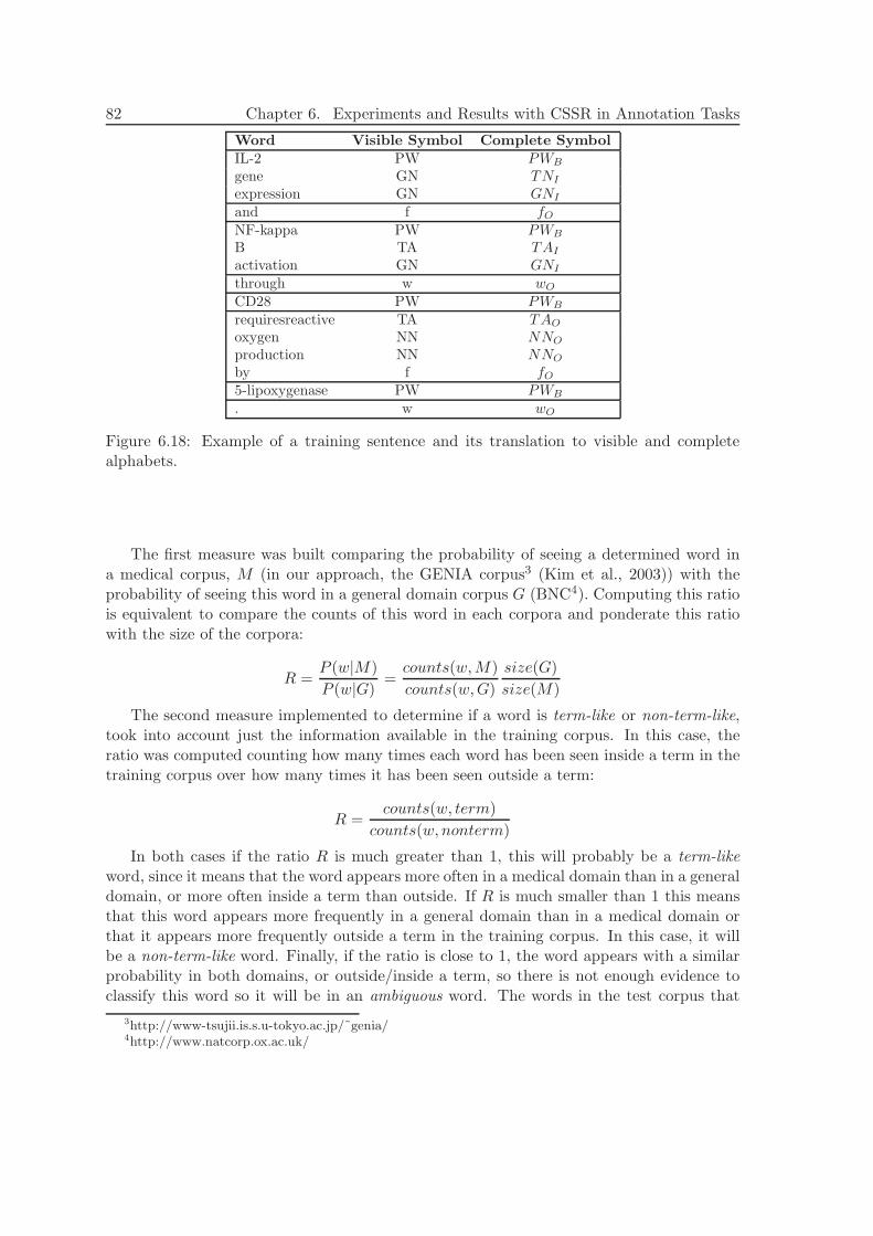
82 Chapter 6. Experiments and Results with CSSR in Annotation Tasks
Word Visible Symbol Complete Symbol
IL-2 PW PWB
gene GN TNI
expression GN GNI
and f fO
NF-kappa PW PWB
B TA TAI
activation GN GNI
through w wO
CD28 PW PWB
requiresreactive TA TAO
oxygen NN NNO
production NN NNO
by f fO
5-lipoxygenase PW PWB
. w wO
Figure 6.18: Example of a training sentence and its translation to visible and completealphabets.
The first measure was built comparing the probability of seeing a determined word ina medical corpus, M (in our approach, the GENIA corpus3 (Kim et al., 2003)) with theprobability of seeing this word in a general domain corpus G (BNC4). Computing this ratiois equivalent to compare the counts of this word in each corpora and ponderate this ratiowith the size of the corpora:
R =P (w|M)
P (w|G)=
counts(w,M)
counts(w,G)
size(G)
size(M)
The second measure implemented to determine if a word is term-like or non-term-like,took into account just the information available in the training corpus. In this case, theratio was computed counting how many times each word has been seen inside a term in thetraining corpus over how many times it has been seen outside a term:
R =counts(w, term)
counts(w,nonterm)
In both cases if the ratio R is much greater than 1, this will probably be a term-likeword, since it means that the word appears more often in a medical domain than in a generaldomain, or more often inside a term than outside. If R is much smaller than 1 this meansthat this word appears more frequently in a general domain than in a medical domain orthat it appears more frequently outside a term in the training corpus. In this case, it willbe a non-term-like word. Finally, if the ratio is close to 1, the word appears with a similarprobability in both domains, or outside/inside a term, so there is not enough evidence toclassify this word so it will be in an ambiguous word. The words in the test corpus that
3http://www-tsujii.is.s.u-tokyo.ac.jp/˜genia/4http://www.natcorp.ox.ac.uk/
6.4. Biomedical Named Entity Recognition 83
have not been seen in the training corpus are also mapped into this last set since there isno evidence to consider them term-like or non-term-like.
To perform the classification in these three sets, two thresholds for R are defined: oneover which a word will be classified as term-like word and another one under which theword will be a non-term-like word. If R is between these two thresholds, the word will beclassified as ambiguous. Lets say sup is the superior threshold for R and inf is the inferiorlimit, then word classification will be:
if R < inf → non-term-like wordif inf < R < sup → ambiguous wordif sup < R → term-like word
The performance of the system is expected to depend strongly on these thresholds thatdetermine the three areas used to classify the words. These thresholds are empiricallydetermined performing the experiments with many different threshold values. Studying theperformance of the system, it was seen that the second measure led to better results thanthe first one. For that reason, the results presented in this work are those obtained withthis second measure.
6.4.3 Experiments and Results
Several experiments to study the influence of the various parameters and to seek for the bestconfiguration were performed. The experiments are conducted with 10-fold cross-validationwith the GENIA 3.0 corpus.
As explained in section 6.4.2, two of the main parameters for this task will be thethresholds to determine if a word is term-like or not. The other important parameters arethe parameters of the algorithm: the maximum length of the histories taken into account(lmax) and the significance level of the hypothesis test. If χ2 test is used to perform thishypothesis test, also the parameter β has to be tuned.
The experiments were originally performed using χ2 test and using only short suffixes todetermine the transient states. In this first experiments, β parameter was set to 1, since thisis the configuration of the original implementation of the algorithm. Secondly we repeatedthe experiments with both χ2 test and Jensen Shannon divergence when using all suffixesto determine recurrent states. In this case, when using χ2 test, β parameter was also tuned.We did not perform the experiments with Jensen Shannon divergence, nor the tuning of βfor χ2 test when using short suffixes to determine recurrent states because we have alreadyseen for NER task that best results are obtained using all suffixes. All the experiments areperformed using sink-1 method.
The best values for precision, recall, and F1 obtained for various maximum lengths andthe values of the parameters that led to these results are presented in the following tables.Table 6.13 shows the results when using χ2 test and short suffixes to determine recurrentstates. In this case, β is set to 1.
In table 6.14 the results obtained with χ2 test and using all suffixes to determine recur-rent states are shown. This table presents both the results obtained using β = 1 and withthe best β.
Finally, table 6.15 shows the best obtained results when using Jensen Shannon diver-gence. In this case, also all suffixes are used to determine recurrent states.
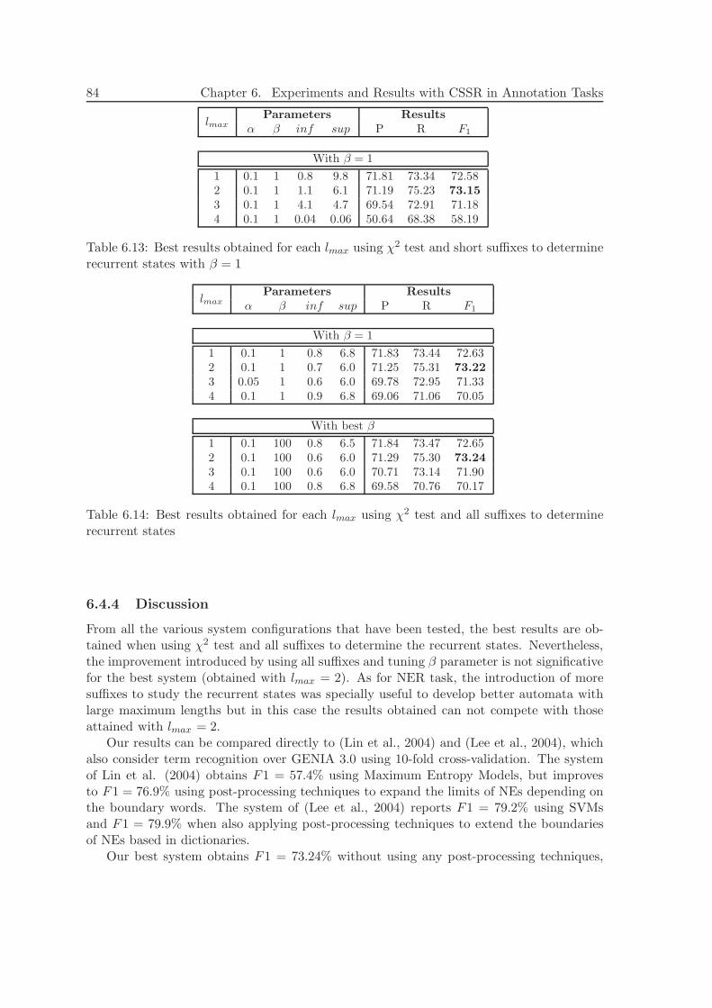
84 Chapter 6. Experiments and Results with CSSR in Annotation Tasks
lmax
Parameters Results
α β inf sup P R F1
With β = 1
1 0.1 1 0.8 9.8 71.81 73.34 72.582 0.1 1 1.1 6.1 71.19 75.23 73.15
3 0.1 1 4.1 4.7 69.54 72.91 71.184 0.1 1 0.04 0.06 50.64 68.38 58.19
Table 6.13: Best results obtained for each lmax using χ2 test and short suffixes to determinerecurrent states with β = 1
lmax
Parameters Results
α β inf sup P R F1
With β = 1
1 0.1 1 0.8 6.8 71.83 73.44 72.632 0.1 1 0.7 6.0 71.25 75.31 73.22
3 0.05 1 0.6 6.0 69.78 72.95 71.334 0.1 1 0.9 6.8 69.06 71.06 70.05
With best β
1 0.1 100 0.8 6.5 71.84 73.47 72.652 0.1 100 0.6 6.0 71.29 75.30 73.24
3 0.1 100 0.6 6.0 70.71 73.14 71.904 0.1 100 0.8 6.8 69.58 70.76 70.17
Table 6.14: Best results obtained for each lmax using χ2 test and all suffixes to determinerecurrent states
6.4.4 Discussion
From all the various system configurations that have been tested, the best results are ob-tained when using χ2 test and all suffixes to determine the recurrent states. Nevertheless,the improvement introduced by using all suffixes and tuning β parameter is not significativefor the best system (obtained with lmax = 2). As for NER task, the introduction of moresuffixes to study the recurrent states was specially useful to develop better automata withlarge maximum lengths but in this case the results obtained can not compete with thoseattained with lmax = 2.
Our results can be compared directly to (Lin et al., 2004) and (Lee et al., 2004), whichalso consider term recognition over GENIA 3.0 using 10-fold cross-validation. The systemof Lin et al. (2004) obtains F1 = 57.4% using Maximum Entropy Models, but improvesto F1 = 76.9% using post-processing techniques to expand the limits of NEs depending onthe boundary words. The system of (Lee et al., 2004) reports F1 = 79.2% using SVMsand F1 = 79.9% when also applying post-processing techniques to extend the boundariesof NEs based in dictionaries.
Our best system obtains F1 = 73.24% without using any post-processing techniques,
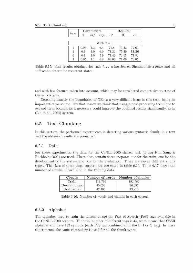
6.5. Text Chunking 85
lmax
Parameters Results
d inf sup P R F1
With β = 1
1 0.05 1.3 6.4 71.8 73.42 72.602 0.1 1.0 6.0 71.22 75.29 73.20
3 0.1 1.0 5.9 71.46 72.15 71.804 0.05 1.1 6.8 69.06 71.06 70.05
Table 6.15: Best results obtained for each lmax using Jensen Shannon divergence and allsuffixes to determine recurrent states
and with few features taken into account, which may be considered competitive to state ofthe art systems.
Detecting exactly the boundaries of NEs is a very difficult issue in this task, being animportant error source. For that reason we think that using a post-processing technique toexpand term boundaries if necessary could improve the obtained results significantly, as in(Lin et al., 2004) system.
6.5 Text Chunking
In this section, the performed experiments in detecting various syntactic chunks in a textand the obtained results are presented.
6.5.1 Data
For these experiments, the data for the CoNLL-2000 shared task (Tjong Kim Sang &Buchholz, 2000) are used. These data contain three corpora: one for the train, one for thedevelopment of the system and one for the evaluation. There are eleven different chunktypes. The sizes of these three corpora are presented in table 6.16. Table 6.17 shows thenumber of chunks of each kind in the training data.
Corpus Number of words Number of chunks
Train 211,794 192,762Development 40,053 36,087Evaluation 47,406 43,210
Table 6.16: Number of words and chunks in each corpus.
6.5.2 Alphabet
The alphabet used to train the automata are the Part of Speech (PoS) tags available inthe CoNLL-2000 corpora. The total number of different tags is 44, what means that CSSRalphabet will have 132 symbols (each PoS tag combined with the B, I or O tag). In theseexperiments, the same vocabulary is used for all the chunk types.
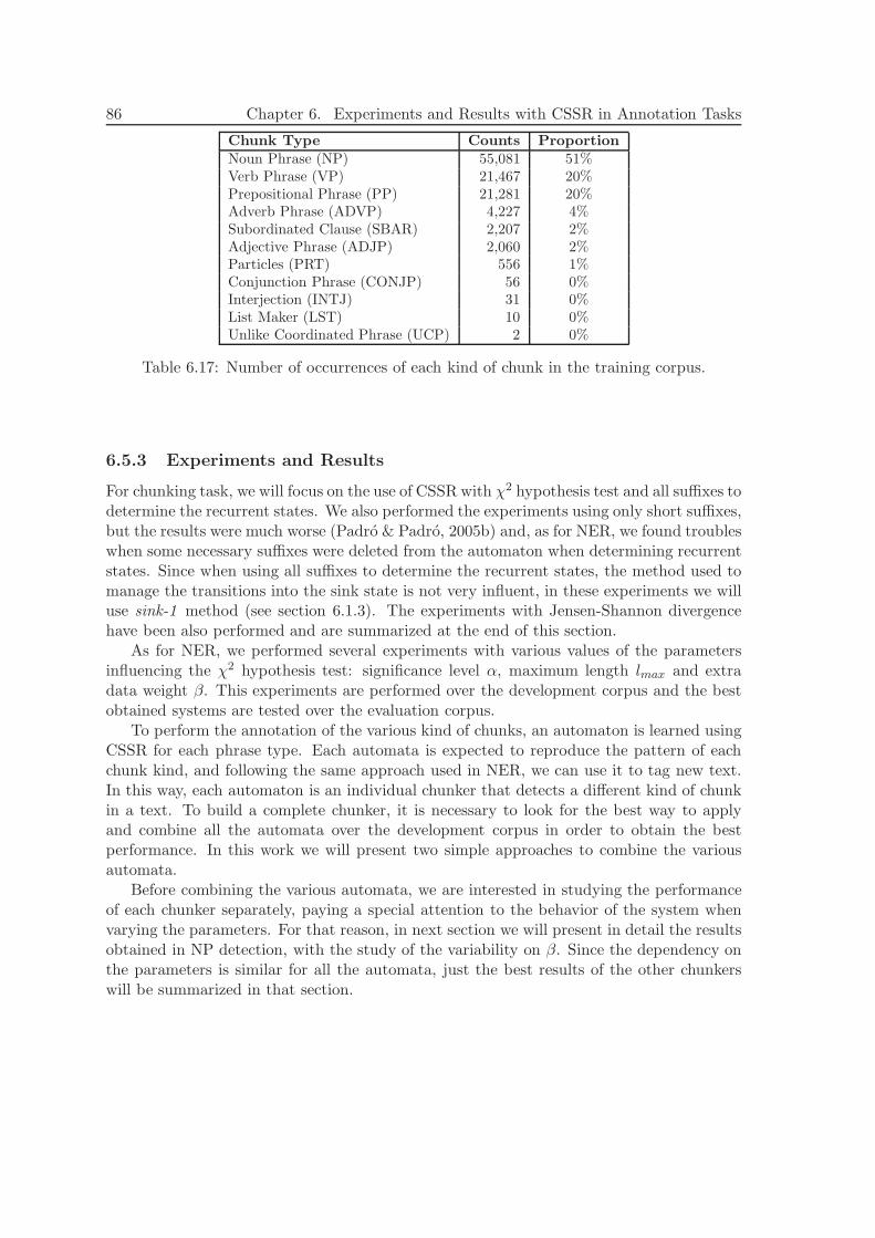
86 Chapter 6. Experiments and Results with CSSR in Annotation Tasks
Chunk Type Counts Proportion
Noun Phrase (NP) 55,081 51%Verb Phrase (VP) 21,467 20%Prepositional Phrase (PP) 21,281 20%Adverb Phrase (ADVP) 4,227 4%Subordinated Clause (SBAR) 2,207 2%Adjective Phrase (ADJP) 2,060 2%Particles (PRT) 556 1%Conjunction Phrase (CONJP) 56 0%Interjection (INTJ) 31 0%List Maker (LST) 10 0%Unlike Coordinated Phrase (UCP) 2 0%
Table 6.17: Number of occurrences of each kind of chunk in the training corpus.
6.5.3 Experiments and Results
For chunking task, we will focus on the use of CSSR with χ2 hypothesis test and all suffixes todetermine the recurrent states. We also performed the experiments using only short suffixes,but the results were much worse (Padro & Padro, 2005b) and, as for NER, we found troubleswhen some necessary suffixes were deleted from the automaton when determining recurrentstates. Since when using all suffixes to determine the recurrent states, the method used tomanage the transitions into the sink state is not very influent, in these experiments we willuse sink-1 method (see section 6.1.3). The experiments with Jensen-Shannon divergencehave been also performed and are summarized at the end of this section.
As for NER, we performed several experiments with various values of the parametersinfluencing the χ2 hypothesis test: significance level α, maximum length lmax and extradata weight β. This experiments are performed over the development corpus and the bestobtained systems are tested over the evaluation corpus.
To perform the annotation of the various kind of chunks, an automaton is learned usingCSSR for each phrase type. Each automata is expected to reproduce the pattern of eachchunk kind, and following the same approach used in NER, we can use it to tag new text.In this way, each automaton is an individual chunker that detects a different kind of chunkin a text. To build a complete chunker, it is necessary to look for the best way to applyand combine all the automata over the development corpus in order to obtain the bestperformance. In this work we will present two simple approaches to combine the variousautomata.
Before combining the various automata, we are interested in studying the performanceof each chunker separately, paying a special attention to the behavior of the system whenvarying the parameters. For that reason, in next section we will present in detail the resultsobtained in NP detection, with the study of the variability on β. Since the dependency onthe parameters is similar for all the automata, just the best results of the other chunkerswill be summarized in that section.
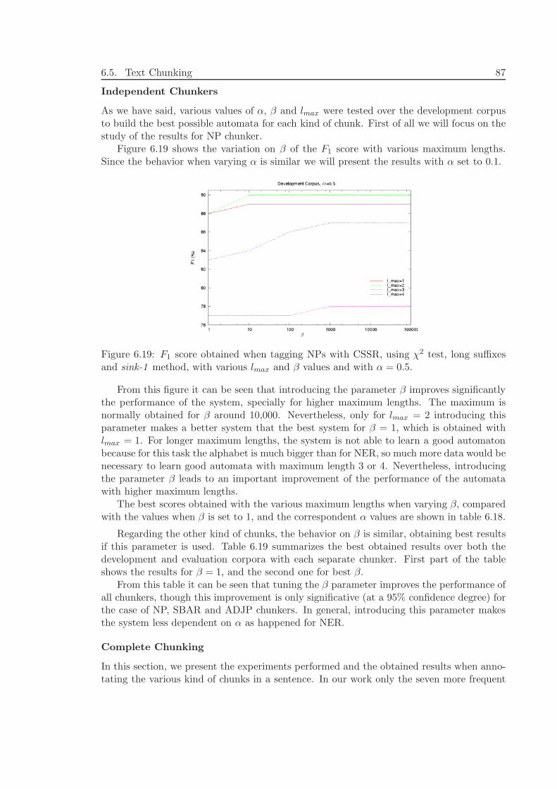
6.5. Text Chunking 87
Independent Chunkers
As we have said, various values of α, β and lmax were tested over the development corpusto build the best possible automata for each kind of chunk. First of all we will focus on thestudy of the results for NP chunker.
Figure 6.19 shows the variation on β of the F1 score with various maximum lengths.Since the behavior when varying α is similar we will present the results with α set to 0.1.
Figure 6.19: F1 score obtained when tagging NPs with CSSR, using χ2 test, long suffixesand sink-1 method, with various lmax and β values and with α = 0.5.
From this figure it can be seen that introducing the parameter β improves significantlythe performance of the system, specially for higher maximum lengths. The maximum isnormally obtained for β around 10,000. Nevertheless, only for lmax = 2 introducing thisparameter makes a better system that the best system for β = 1, which is obtained withlmax = 1. For longer maximum lengths, the system is not able to learn a good automatonbecause for this task the alphabet is much bigger than for NER, so much more data would benecessary to learn good automata with maximum length 3 or 4. Nevertheless, introducingthe parameter β leads to an important improvement of the performance of the automatawith higher maximum lengths.
The best scores obtained with the various maximum lengths when varying β, comparedwith the values when β is set to 1, and the correspondent α values are shown in table 6.18.
Regarding the other kind of chunks, the behavior on β is similar, obtaining best resultsif this parameter is used. Table 6.19 summarizes the best obtained results over both thedevelopment and evaluation corpora with each separate chunker. First part of the tableshows the results for β = 1, and the second one for best β.
From this table it can be seen that tuning the β parameter improves the performance ofall chunkers, though this improvement is only significative (at a 95% confidence degree) forthe case of NP, SBAR and ADJP chunkers. In general, introducing this parameter makesthe system less dependent on α as happened for NER.
Complete Chunking
In this section, we present the experiments performed and the obtained results when anno-tating the various kind of chunks in a sentence. In our work only the seven more frequent
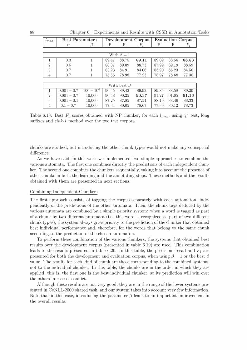
88 Chapter 6. Experiments and Results with CSSR in Annotation Tasks
lmax Best Parameters Development Corpus Evaluation Corpus
α β P R F1 P R F1
With β = 11 0.3 1 89.47 88.75 89.11 89.09 88.56 88.83
2 0.5 1 88.37 89.09 88.73 87.99 89.19 88.593 0.7 1 83.23 84.91 84.06 83.90 85.23 84.564 0.7 1 75.55 78.98 77.23 75.97 78.68 77.30
With best β1 0.001 – 0.7 100 – 106 90.45 89.42 89.93 89,84 88.58 89.202 0.001 – 0.7 10,000 90.48 90.25 90.37 91.27 91.05 91.16
3 0.001 – 0.1 10,000 87.25 87.85 87.54 88.19 88.46 88.334 0.1 – 0.7 10,000 77.34 80.05 78.67 77.39 80.12 78.73
Table 6.18: Best F1 scores obtained with NP chunker, for each lmax, using χ2 test, longsuffixes and sink-1 method over the two test corpora.
chunks are studied, but introducing the other chunk types would not make any conceptualdifference.
As we have said, in this work we implemented two simple approaches to combine thevarious automata. The first one combines directly the predictions of each independent chun-ker. The second one combines the chunkers sequentially, taking into account the presence ofother chunks in both the learning and the annotating steps. These methods and the resultsobtained with them are presented in next sections.
Combining Independent Chunkers
The first approach consists of tagging the corpus separately with each automaton, inde-pendently of the predictions of the other automata. Then, the chunk tags deduced by thevarious automata are combined by a simple priority system: when a word is tagged as partof a chunk by two different automata (i.e. this word is recognized as part of two differentchunk types), the system always gives priority to the prediction of the chunker that obtainedbest individual performance and, therefore, for the words that belong to the same chunkaccording to the prediction of the chosen automaton.
To perform these combination of the various chunkers, the systems that obtained bestresults over the development corpus (presented in table 6.19) are used. This combinationleads to the results presented in table 6.20. In this table, the precision, recall and F1 arepresented for both the development and evaluation corpus, when using β = 1 or the best βvalue. The results for each kind of chunk are those corresponding to the combined systems,not to the individual chunker. In this table, the chunks are in the order in which they areapplied, this is, the first one is the best individual chunker, so its prediction will win overthe others in case of conflict.
Although these results are not very good, they are in the range of the lower systems pre-sented in CoNLL-2000 shared task, and our system takes into account very few information.Note that in this case, introducing the parameter β leads to an important improvement inthe overall results.
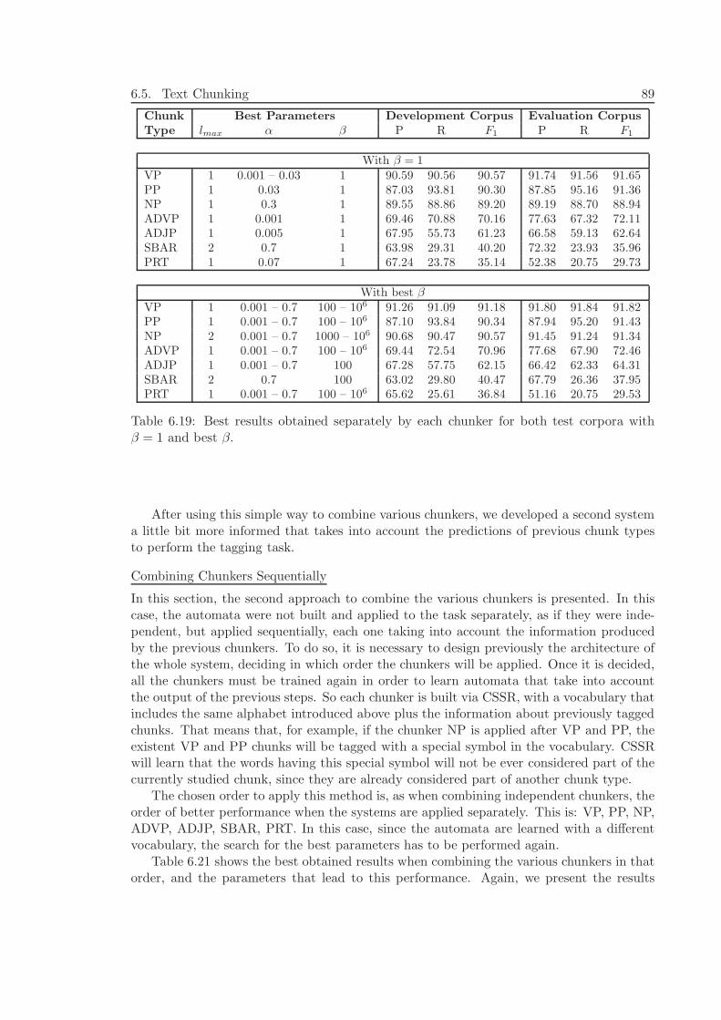
6.5. Text Chunking 89
Chunk Best Parameters Development Corpus Evaluation Corpus
Type lmax α β P R F1 P R F1
With β = 1VP 1 0.001 – 0.03 1 90.59 90.56 90.57 91.74 91.56 91.65PP 1 0.03 1 87.03 93.81 90.30 87.85 95.16 91.36NP 1 0.3 1 89.55 88.86 89.20 89.19 88.70 88.94ADVP 1 0.001 1 69.46 70.88 70.16 77.63 67.32 72.11ADJP 1 0.005 1 67.95 55.73 61.23 66.58 59.13 62.64SBAR 2 0.7 1 63.98 29.31 40.20 72.32 23.93 35.96PRT 1 0.07 1 67.24 23.78 35.14 52.38 20.75 29.73
With best βVP 1 0.001 – 0.7 100 – 106 91.26 91.09 91.18 91.80 91.84 91.82PP 1 0.001 – 0.7 100 – 106 87.10 93.84 90.34 87.94 95.20 91.43NP 2 0.001 – 0.7 1000 – 106 90.68 90.47 90.57 91.45 91.24 91.34ADVP 1 0.001 – 0.7 100 – 106 69.44 72.54 70.96 77.68 67.90 72.46ADJP 1 0.001 – 0.7 100 67.28 57.75 62.15 66.42 62.33 64.31SBAR 2 0.7 100 63.02 29.80 40.47 67.79 26.36 37.95PRT 1 0.001 – 0.7 100 – 106 65.62 25.61 36.84 51.16 20.75 29.53
Table 6.19: Best results obtained separately by each chunker for both test corpora withβ = 1 and best β.
After using this simple way to combine various chunkers, we developed a second systema little bit more informed that takes into account the predictions of previous chunk typesto perform the tagging task.
Combining Chunkers Sequentially
In this section, the second approach to combine the various chunkers is presented. In thiscase, the automata were not built and applied to the task separately, as if they were inde-pendent, but applied sequentially, each one taking into account the information producedby the previous chunkers. To do so, it is necessary to design previously the architecture ofthe whole system, deciding in which order the chunkers will be applied. Once it is decided,all the chunkers must be trained again in order to learn automata that take into accountthe output of the previous steps. So each chunker is built via CSSR, with a vocabulary thatincludes the same alphabet introduced above plus the information about previously taggedchunks. That means that, for example, if the chunker NP is applied after VP and PP, theexistent VP and PP chunks will be tagged with a special symbol in the vocabulary. CSSRwill learn that the words having this special symbol will not be ever considered part of thecurrently studied chunk, since they are already considered part of another chunk type.
The chosen order to apply this method is, as when combining independent chunkers, theorder of better performance when the systems are applied separately. This is: VP, PP, NP,ADVP, ADJP, SBAR, PRT. In this case, since the automata are learned with a differentvocabulary, the search for the best parameters has to be performed again.
Table 6.21 shows the best obtained results when combining the various chunkers in thatorder, and the parameters that lead to this performance. Again, we present the results
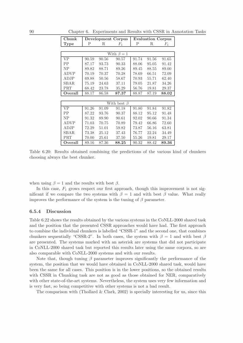
90 Chapter 6. Experiments and Results with CSSR in Annotation Tasks
Chunk Development Corpus Evaluation Corpus
Type P R F1 P R F1
With β = 1VP 90.59 90.56 90.57 91.74 91.56 91.65PP 87.17 93.73 90.33 88.06 95.05 91.42NP 89.82 88.71 89.26 89.45 88.55 89.00ADVP 70.19 70.37 70.28 78.69 66.51 72.09ADJP 69.88 50.56 58.67 70.93 55.71 62.40SBAR 75.19 24.63 37.11 79.05 21.87 34.26PRT 68.42 23.78 35.29 56.76 19.81 29.37Overall 88.17 86.58 87.37 88.87 87.19 88.02
With best βVP 91.26 91.09 91.18 91.80 91.84 91.82PP 87.22 93.76 90.37 88.12 95.12 91.48NP 91.32 89.90 90.61 92.02 90.66 91.34ADVP 71.03 70.75 70.89 79.42 66.86 72.60ADJP 72.29 51.01 59.82 73.87 56.16 63.81SBAR 73.38 25.12 37.43 76.77 22.24 34.49PRT 70.00 25.61 37.50 55.26 19.81 29.17Overall 89.16 87.36 88.25 90.32 88.42 89.36
Table 6.20: Results obtained combining the predictions of the various kind of chunkerschoosing always the best chunker.
when using β = 1 and the results with best β.In this case, F1 grows respect our first approach, though this improvement is not sig-
nificant if we compare the two systems with β = 1 and with best β value. What reallyimproves the performance of the system is the tuning of β parameter.
6.5.4 Discussion
Table 6.22 shows the results obtained by the various systems in the CoNLL-2000 shared taskand the position that the presented CSSR approaches would have had. The first approachto combine the individual chunkers is labelled “CSSR-1” and the second one, that combineschunkers sequentially “CSSR-2”. In both cases, the system with β = 1 and with best βare presented. The systems marked with an asterisk are systems that did not participatein CoNLL-2000 shared task but reported this results later using the same corpora, so arealso comparable with CoNLL-2000 systems and with our results.
Note that, though tuning β parameter improves significantly the performance of thesystem, the position that we would have obtained in CoNLL-2000 shared task, would havebeen the same for all cases. This position is in the lower positions, so the obtained resultswith CSSR in Chunking task are not as good as those obtained for NER, comparativelywith other state-of-the-art systems. Nevertheless, the system uses very few information andis very fast, so being competitive with other systems is not a bad result.
The comparison with (Thollard & Clark, 2002) is specially interesting for us, since this
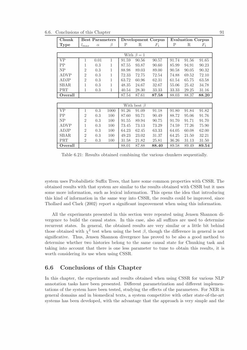
6.6. Conclusions of this Chapter 91
Chunk Best Parameters Development Corpus Evaluation Corpus
Type lmax α β P R F1 P R F1
With β = 1VP 1 0.01 1 91.59 90.56 90.57 91.74 91.56 91.65PP 1 0.3 1 87.55 93.87 90.60 85.99 94.91 90.23NP 2 0.3 1 88.98 89.03 89.00 90.58 90.05 90.32ADVP 2 0.3 1 72.33 72.75 72.54 74.88 69.52 72.10ADJP 2 0.3 1 63.72 60.96 62.31 61.54 65.75 63.58SBAR 1 0.3 1 48.35 24.67 32.67 55.06 25.42 34.78PRT 1 0.3 1 40.54 28.30 33.33 33.33 29.25 31.16Overall 87.54 87.61 87.58 88.03 88.37 88.20
With best βVP 1 0.3 1000 91.26 91.09 91.18 91.80 91.84 91.82PP 2 0.3 100 87.60 93.71 90.49 88.72 95.06 91.76NP 2 0.3 100 91.55 89.94 90.75 91.70 91.71 91.70ADVP 1 0.3 100 73.45 73.13 73.29 74.59 77.26 75.90ADJP 2 0.3 100 64.23 62.45 63.33 64.05 60.08 62.00SBAR 2 0.3 100 49.23 23.02 31.37 64.25 21.50 32.21PRT 2 0.3 100 31.58 21.82 25.81 36.26 31.13 31.50Overall 88.01 87.88 88.40 89.58 89.49 89.54
Table 6.21: Results obtained combining the various chunkers sequentially.
system uses Probabilistic Suffix Trees, that have some common properties with CSSR. Theobtained results with that system are similar to the results obtained with CSSR but it usessome more information, such as lexical information. This opens the idea that introducingthis kind of information in the same way into CSSR, the results could be improved, sinceThollard and Clark (2002) report a significant improvement when using this information.
All the experiments presented in this section were repeated using Jensen Shannon di-vergence to build the causal states. In this case, also all suffixes are used to determinerecurrent states. In general, the obtained results are very similar or a little bit behindthose obtained with χ2 test when using the best β, though the difference in general is notsignificative. Thus, Jensen Shannon divergence has proved to be also a good method todetermine whether two histories belong to the same causal state for Chunking task andtaking into account that there is one less parameter to tune to obtain this results, it isworth considering its use when using CSSR.
6.6 Conclusions of this Chapter
In this chapter, the experiments and results obtained when using CSSR for various NLPannotation tasks have been presented. Different parametrization and different implemen-tations of the system have been tested, studying the effects of the parameters. For NER ingeneral domains and in biomedical texts, a system competitive with other state-of-the-artsystems has been developed, with the advantage that the approach is very simple and the
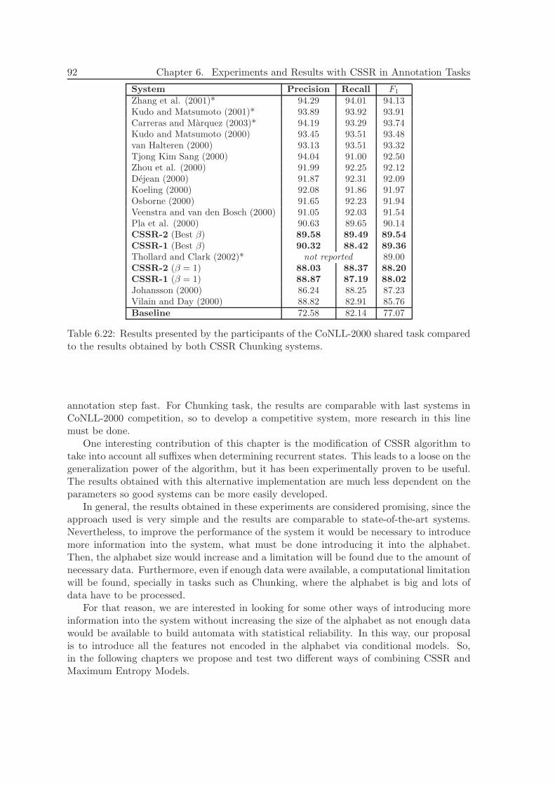
92 Chapter 6. Experiments and Results with CSSR in Annotation Tasks
System Precision Recall F1
Zhang et al. (2001)* 94.29 94.01 94.13Kudo and Matsumoto (2001)* 93.89 93.92 93.91Carreras and Marquez (2003)* 94.19 93.29 93.74Kudo and Matsumoto (2000) 93.45 93.51 93.48van Halteren (2000) 93.13 93.51 93.32Tjong Kim Sang (2000) 94.04 91.00 92.50Zhou et al. (2000) 91.99 92.25 92.12Dejean (2000) 91.87 92.31 92.09Koeling (2000) 92.08 91.86 91.97Osborne (2000) 91.65 92.23 91.94Veenstra and van den Bosch (2000) 91.05 92.03 91.54Pla et al. (2000) 90.63 89.65 90.14CSSR-2 (Best β) 89.58 89.49 89.54
CSSR-1 (Best β) 90.32 88.42 89.36
Thollard and Clark (2002)* not reported 89.00CSSR-2 (β = 1) 88.03 88.37 88.20
CSSR-1 (β = 1) 88.87 87.19 88.02
Johansson (2000) 86.24 88.25 87.23Vilain and Day (2000) 88.82 82.91 85.76Baseline 72.58 82.14 77.07
Table 6.22: Results presented by the participants of the CoNLL-2000 shared task comparedto the results obtained by both CSSR Chunking systems.
annotation step fast. For Chunking task, the results are comparable with last systems inCoNLL-2000 competition, so to develop a competitive system, more research in this linemust be done.
One interesting contribution of this chapter is the modification of CSSR algorithm totake into account all suffixes when determining recurrent states. This leads to a loose on thegeneralization power of the algorithm, but it has been experimentally proven to be useful.The results obtained with this alternative implementation are much less dependent on theparameters so good systems can be more easily developed.
In general, the results obtained in these experiments are considered promising, since theapproach used is very simple and the results are comparable to state-of-the-art systems.Nevertheless, to improve the performance of the system it would be necessary to introducemore information into the system, what must be done introducing it into the alphabet.Then, the alphabet size would increase and a limitation will be found due to the amount ofnecessary data. Furthermore, even if enough data were available, a computational limitationwill be found, specially in tasks such as Chunking, where the alphabet is big and lots ofdata have to be processed.
For that reason, we are interested in looking for some other ways of introducing moreinformation into the system without increasing the size of the alphabet as not enough datawould be available to build automata with statistical reliability. In this way, our proposalis to introduce all the features not encoded in the alphabet via conditional models. So,in the following chapters we propose and test two different ways of combining CSSR andMaximum Entropy Models.
CHAPTER 7
Extending CSSR with ME models
In previous chapters, it has been seen that using CSSR for NLP tasks leads to reasonablygood results, specially taking into account the simplicity of the considered features. Theproblem is that the proposed approach is rather limited, since all information we wantto take into account has to be encoded in the alphabet, so if we want to introduce moresophisticated features into the system to try to improve the performance, the alphabetsize will grow. But since the amount of necessary data to build a correct automaton growsexponentially with the alphabet size, it is important not to increase the alphabet size beyondthe limit established by the available data.
For that reason, the improvement of the performance of the system is tied to introducingmore information into the system without increasing the alphabet size. In this line, wepropose to combine CSSR algorithm with conditional models that can take into accountmore complicated information. Thus, the generative model of CSSR would be convertedinto a conditional model. Two examples of conditional models that could be used in thisway are Conditional Random Fields (Lafferty et al., 2001; Wallach, 2004) or MaximumEntropy (ME) Models (Berger et al., 1996; Ratnaparkhi, 1997).
Convining conditional models with CSSR we expect to take advantage of the power ofconditional models, for example the ability to take many features into account and also touse the good properties of CSSR such as it builds markovian automata that are minimal,so we can encode the same information than a Markov Model encodes but with much lessmemory.
We focus on the use of ME models with CSSR because McCallum et al. (2000) alreadyapproached a way of combining these models with Hidden Markov Models, named Maxi-mum Entropy Markov Models (MEMM) obtaining good results in the field of InformationExtraction. Since CSSR builds automata similar to Markov Models, we think that it isinteresting to try to combine it with ME models in a similar way than MEMMs do. Ne-vertheless, our proposal can not be directly compared to MEMMs since they use HiddenMarkov Models and our approach uses CSSR automata that do not directly include hiddeninformation.
This chapter first of all introduces the Maximum Entropy Models framework (section
93
94 Chapter 7. Extending CSSR with ME models
7.1) and then presents, in section 7.2, the proposed approaches to combine ME models andCSSR. We will present two different systems and a baseline that will be tested in chapter 8in NER task.
7.1 Maximum Entropy Models
Maximum Entropy (ME) models (Berger et al., 1996; Ratnaparkhi, 1997) offer a way toestimate the probability of a determined linguistic class given a linguistic context. Theintuitive idea behind these models is to look for the most uniform probability distributionthat satisfies all the constraints (context). This is equivalent to say that the model fulfills theconstraints but makes the fewest possible assumptions. This uniformity of the distributioncan be measured with the entropy, the higher the entropy, the more uniform the distribution.Thus, the Maximum Entropy models are constructed in order that the computed probabilitymaximizes the entropy of the model, while keeping it consistent with the observation.
Consider A the set of all possible classes and B the set of all possible contexts. Thenwe can define a ∈ A, b ∈ B and the probability of a in context b will be p(a|b). When theseprobabilities are estimated from data, we denote p(a, b) the estimated probability for thepair (a, b).
7.1.1 Representing Context and Constraints
To represent the evidence, this is, the context of an observation, all relevant informationis encoded into features, that take into account the useful information of the system. Foreach task, various features will be relevant. Each feature is a binary function of the currentclass and the context f(a, b) that is set to one when certain values of a and b occur and iszero in any other case. When f(a, b) = 1, we will say that the feature is active.
Thus, all the relevant information useful to model the system must be translated intofeature functions creating a feature set fi. To ensure that the model takes into account thisinformation, the expected value p(f) that the model assigns to the corresponding featurefunction f is constrained with the f value for each (a, b) pair:
p(f) =∑
a∈A, b∈B
p(a, b)f(a, b) =∑
a∈A, b∈B
p(b)p(a|b)f(a, b)
where p(b) is the empirical distribution of b in the training sample. Then, the constraintour model has to fulfill is that its estimated probability p(f) is equal to the real probabilityp(f). There will be various models p(a|b) consistent with these constraints, but following thePrinciple of Maximum Entropy (Jaynes, 1957; Good, 1963) we look for the model p∗(a|b)that maximizes the entropy H(p):
H(p) ≡ −∑
a∈A, b∈B
p(b)p(a|b) log p(a|b)
remaining consistent with the evidence. Thus the selected model will be
p∗ = argmaxpH(p)
7.2. Introducing ME models into CSSR 95
7.1.2 Parametric Form
Given a real corpus and a set of features, the task of determining which is the model thatsatisfies the constraints and maximizes the entropy is not trivial. The most usual approachis to use the method of Lagrange multipliers to estimate this best model. Here we willsummarize the basic ideas of this technique, for a more detailed explanation see (Bergeret al., 1996; Ratnaparkhi, 1997; Della Pietra et al., 1997).
The basic idea is that each feature fi has a Lagrange multiplier λi associated calledweight. Then we can define a Lagrangian function Λ(p, λ) that must be maximized tomaximize the entropy. Then, it can be demonstrated that the model that maximizes theentropy is a function of the features and its weights:
pλ(a|b) =1
Zλ(b)exp
(
∑
i
λifi(a, b)
)
where Zλ(b) is a normalization constant that mantains the probability distribution normal-ized and is computed as
Zλ(b) =∑
a
exp
(
∑
i
λifi(a, b)
)
This way of computing p(a|b) is called parametric form and is used to compute proba-bilities once the various weights λ for each feature and each class are estimated. There isa variety of algorithms to estimate λ values such as Generalized Iterative Scaling (Darroch& Ratcliff, 1972), Improved Iterative Scaling (Della Pietra et al., 1997) or Limited MemoryBFGS (Daume III, 2004). This last algorithm is the one that will be used in this work. Fora comparison of some of these algorithms, see (Malouf, 2002a).
Given a data set, what these algorithms do is to estimate the weights of each featurefor each class that maximize the entropy fulfilling the constraints. Once these weights havebeen determined, they can be used to estimate the probability of any class in any contextwhich is, in fact, what is needed to process new examples.
7.2 Introducing ME models into CSSR
As we have said, our main goal is to introduce into CSSR information that is not encoded inthe alphabet. In this way, the algorithm should be able to build more informed automatonwithout suffering the problems of increasing the alphabet size while having a limited amountof data.
As discussed before, there are various conditional models that would be suitable forthe proposed approach, but in this work we focus on the use of Maximum Entropy modelsto compute the probability distribution of the future. The classes of ME models are thesymbols of the complete alphabet used with CSSR, and they define the possible transitionsof each state in the automaton. The relevant information associated to each word is encodedin a variety of features, and ME models are used to compute the probability distribution ofthe next symbol given the current active features.
For example, considering the alphabet used for NER in section 6.3, with CSSR theprobability to be computed had the form of P (MB |SBaIwO), but now the probability will

96 Chapter 7. Extending CSSR with ME models
be computed as P (MB |h) where h is a history including the symbols and relevant featuresof last words.
7.2.1 Methodology
In order to study the performance of ME models in the approached NLP tasks and oftheir combination with CSSR, we present two different approaches to combine these twoalgorithms: ME-over-CSSR and ME-CSSR. Also, a baseline method (Plain-ME) will beused, that uses ME models but does not combine them with CSSR.
All these methods have in common that they need an ME model learned taking intoaccount the relevant features of the task. Also, all of them will use the symbols of thecomplete alphabet as the classes of the model.
To build ME models, it is necessary, first of all, to define the feature set relevant foreach concrete task. Once it has been done, the features for each word in each corporaand the corresponding class (which corresponds to a symbol of the complete alphabet) areextracted. In our work, we do that using libfries-0.93, which is part of FreeLing analyzer(Carreras et al., 2004; Atserias et al., 2006)1 and based on (Cumby & Roth, 2003). Oncethe corpora are encoded in that way, the training corpus is used to learn the MaximumEntropy model, this is, the weights for each feature and each class. In our case, this isperformed with MEGA Model Optimization Package (Daume III, 2004)2.
In next sections we describe the two approaches used in this work to combine ME modelsand CSSR, as well as the baseline method.
7.2.2 Plain ME
This first approach will be used as a baseline of ME models performance since, in fact, itdoes not use CSSR in any way.
The idea of this first method it to use the learned ME models to compute the probabilityof each word in test corpus of having each possible class. It has to be taken into accountthat there is a known part of the symbol (e.g. we know if it is G, M , w, etc.), so the possibleclasses will be three, one for each possible B, I, O tag. For example, if we know that theword has the visible symbol M , the probability of seeing this word in this context with thecomplet symbol MB, MI and MO will be computed using the ME model.
Then, with these probabilities computed, the most likely sequence of tags is computedusing the Viterbi algorithm, following a similar approach to the one used by Ratnaparkhi(1996).
7.2.3 ME-over-CSSR
This is a first proposal to combine CSSR and ME models without changing the algorithmitself. This method is fast and simple, and we use it to see if introducing more informa-tion into the system with ME models leads to better results than using both techniquesseparately.
1FreeLing: Software and information available at http://www.lsi.upc.edu/˜nlp/freeling2MEGAM: Software and information available at http://www.cs.utah.edu/˜hal/megam
7.2. Introducing ME models into CSSR 97
Building the Automaton
The method consists of using CSSR to learn an automaton as in chapter 5, using a simplealphabet that includes the hidden information. So in the automaton building step, MEmodels are not used. The model is used only during the annotation task, to refine thetransition probabilities.
Annotating New Text
To annotate new sentences with ME-over-CSSR, a Viterbi algorithm using CSSR learnedautomaton is used, as explained in section 5.3. But in this case, the transition probabilityfor a word with a symbol a is computed as a linear combination of the transition probabilityfor the current state s given by CSSR automaton and the probability computed with theME model taking into account the features of the studied word (F = {f1, f2, ...fn}):
P (a|s, F ) = µ · PCSSR(a|s) + (1 − µ) · PME(a|F )
In this way, we combine the power of the ME models, that are expected to give moreaccurate probabilities given the real context, and the information encoded in the automaton,that can, for example, forbid some transition between states or provide information notcaptured by the ME models. Note that this way of computing P (a|s, F ) includes the twolimit cases: if µ = 0, we are taking into account just the probability of the ME model, so weare not using the automaton at all. This will be equivalent to perform directly the Viterbialgorithm using ME models as in the method “Plain ME”. On the other hand, if µ = 1, justthe probability of the state is used, so it is equivalent to use CSSR without ME models.
Managing Unseen Transitions
As for normal CSSR, when performing the annotation task, there can be symbol com-binations that has not been seen in the training corpus and the automaton would fall intoa sink state. Then, it is necessary to implement some method to evolute to a known stateand continue tagging the sentence normally.
For ME-over-CSSR we have used the same methods for dealing with the sink statepresented in section 5.4. The difference between this process for CSSR and for ME-over-CSSR is that in the first case, while the system is in the sink state there is no informationabout the probabilities each possible symbol can have. Nevertheless, when using ME-over-CSSR, if we are in the sink state we still can compute the probability for each symbolgiven the context using the ME model so we have more information to tag correctly theunknown word that when using simple CSSR. This makes the problem of falling into thesink state less important and the difference between the two sink methods tested for NERnot significant.
7.2.4 ME-CSSR
In this approach, CSSR is modified to include the use of ME models in both the stepof building the automaton and the annotation task. The main idea of this approach isbased on generalizing the concept of history. Instead of considering histories as sequencesof alphabet symbols corresponding to the last lmax words, we define histories as sets ofrelevant information about the last lmax words. Thus, histories can be encoded as collectionsof features of the words in a window of size lmax. Then, causal states can still be defined as
98 Chapter 7. Extending CSSR with ME models
sets of histories with the same distribution for the future and can be calculated followingthe structure of CSSR.
In this way, all the information encoded in the features is taken into account whenbuilding the automaton and the automaton is expected to better capture the patterns ofsequences since it has more information.
Building the automaton with ME-CSSR
Once the histories are extended to be sets of features rather than simple suffixes, the al-gorithm for building the automaton is conceptually similar to the original CSSR but withsome variations:
• As in CSSR, the transitions between states are labelled with the complete symbolalphabet (including the hidden tag), as it is necessary to have a closed and reducednumber of transitions. Then, the probability distribution of a history is P (a|x−) wherea is a symbol of the complete alphabet and x− is a history represented as a set offeatures.
• Probability distributions for each history are computed using Maximum Entropy mo-dels, instead of Maximum Likelihood as original CSSR does. To do so it is necessaryto extract the feature set for each word in the training corpus and compute the MEmodels before executing ME-CSSR. With this models ME-CSSR can compute theprobability distribution of the histories and compare it with the distribution of thevarious causal states using a hypothesis test such as χ2 test or a distribution distancesuch as Jensen Shannon distance (Lin, 1991).
• In Sufficiency step, CSSR builds iteratively all possible suffixes and compares theirprobability distributions with existing causal states. ME-CSSR can not do that as theconsidered features may not be a closed set. Then, sufficiency is performed studyingall histories that have been seen in the training corpus, from length 1 to lmax .
• The automaton built using ME-CSSR is not deterministic, but this is not a problem forannotation tasks, since Viterbi algorithm can explore all possible paths and choosethe best one. The causal state machine is not deterministic not only because twohistories with the same probability distribution for the future can evolute to differentstates with a given symbol, but also because there can be multiple transitions for aconcrete history. For example, consider the history formed by the features of threeconsecutive words (lmax = 3):
w1 : F1 = {f11 f2
1 f31 ...}
w2 : F2 = {f12 f2
2 f32 ...}
w3 : F3 = {f13 f2
3 f33 ...}
The history h1 is formed by all the features of the last three words: F1F2F3, andwith a given symbol a will evolute to F2F3F4, where F4 is the set of features for thenext word, including the symbol a. Note that the first word disappears because themaximum considered length is 3. The only thing that we know about the historyreceiving the transition is that its last symbol must be a, but there can be different
7.2. Introducing ME models into CSSR 99
valid values of all other features for last position F4. Thus there can be various existinghistories in various states receiving the transitions of history h1 with symbol a, andit is not possible to make it deterministic by splitting histories in different states asCSSR does since a single history makes the automaton indeterministic. Even a statewith just one history would have different possible transitions for each symbol.
Annotation Tasks with ME-CSSR
When the annotation task is to be performed with the learned automaton, the same ap-proach presented in section 5.3 is applied. Thus, the alphabet used for the transitionscontains the hidden information and a Viterbi algorithm is applied to determine the mostlikely symbol sequence which is the best B-I-O tag sequence.
In this case, the difference is that the states and their transitions already encode in-formation about more complicated features. Nevertheless, it is still interesting to use notonly the probabilities for the states but also the real features of the word we are tagging tocompute the probability of seeing each symbol. In this way, we take maximum advantageof the learned ME models and the information encoded in them. So, in the annotation taskthe ME model is also used to compute the probability of seeing each symbol (class) giventhe current context.
As for ME-over-CSSR, to obtain the probability of a determined symbol given a wordwith its context and being in a state of the automaton, the probability given by the MEmodel is combined (with a weight µ) with the probability given by the state.
In this way, we have a global transition probability that takes into account both theinformation of the ME model and of CSSR. The idea is that there can be informationencoded in the automaton that can not be encoded in the ME models, and vice versa.Again, if µ = 0, the system will perform equivalently to the method “Plain ME” and ifµ = 1, only the transition probabilities of the automaton will be used, tough in this case,this will not be equivalent to CSSR as the states are formed by more complicated histories.
Several experiments with various values of µ will be performed to see the behavior ofthe annotation system in the case of both methods.
Managing Unseen Transitions
In this case, to solve the problem of falling into the sink state, it is not possible to usethe same approach used for the basic CSSR or for ME-over-CSSR, where the basic idea wasto search for similar suffixes in other states or to wait for a known suffixes, as, if the featureset is complicated enough, there will be lots of unseen histories and waiting for a historyequal to some history present in the automaton could take a long time.
Thus, we propose to compare the probability distribution of the current (and unseen)history, computed using the ME model, with all the states in the automaton. This is thesame procedure that ME-CSSR does when building the automaton to determine which stateeach history belongs to. Then, the system evolves to those states that pass the test withthe same confidence degree used to learn the automaton.
If no state passes the test, the path is continued using only the ME computed probabilityand the same operation is performed with next word until the system finds a suitable statefor the new history.

100 Chapter 7. Extending CSSR with ME models
7.3 Conclusions of this Chapter
At the sight of the results presented in chapter 6, it was seen that the approach proposedto apply CSSR to annotation NLP tasks had some limitations due to the limited amount ofavailable data and to the complicated nature of such tasks. For that reason, two methods tocombine CSSR algorithm with ME models have been devised and presented in this chapter.Next chapter presents the performed experiments with these two methods and with thebaseline method, in NER task. In the future, other tasks will be also approached with thesemethods.
CHAPTER 8
Experiments and Results with ME-extended CSSR
The two methods and the baseline presented in chapter 7 have been tested in the task ofNamed Entity Recognition (NER).
Regarding ME-CSSR, first experiments were performed using χ2 hypothesis test, andsome preliminary results were presented in FSMNLP’07 workshop (Padro & Padro, 2007a).Nevertheless, these preliminary results, and the study of the error sources showed that thistest is not suitable when using ME-CSSR, as we will explain in section 8.3. For that reasonwe used Jensen Shannon divergence to compare future distributions. The experiments andresults obtained with this system, performed with more complicated features are presentedin this chapter, and are under review for publication.
8.1 Data and Alphabet
As we have said, the data and alphabet used for NER task with ME-extended CSSR arethe same used for the task with CSSR alone. This is, the data are those of CoNLL-2002shared task (Tjong Kim Sang, 2002a), that have a train corpus and two test corpora andthe visible alphabet has 5 symbols which combined with the B-I-O tags lead to a 15 symbolcomplete alphabet.
8.2 Features
To use the different proposed methods to combine ME and CSSR, it is necessary to definethe relevant features for the task.
For the development step, different combinations of some relevant features were testedover the development corpus. For each feature set, the features that appear less are filtered,testing also various filter levels to obtain the best possible model. Furthermore, each modelis tested using different parametrization that can affect the performance of the method. Theparameters to be tuned for the methods that use ME models and CSSR are: the maximum
101
102 Chapter 8. Experiments and Results with ME-extended CSSR
length of the histories, the significance degree of the hypothesis test and the ponderationvalue for the annotation step µ.
Many combinations of various features were used and tested with these methods, herewe summarize the features that led to best results. The features we use include informationabout the words in the sentence, their orthography, their Part of Speech tag and their BIOtag.
All the best feature sets include a basic set of features that we will call Basic formedby: word, lemma, PoS tag, sentence-end mark, visible symbol, complete symbol and BIO-tag. Note that for the last two features this information is available in the training corpus,which is necessary to build the models, but not in the test corpus. So, when performingthe annotation step, the feature used for the hidden information is the one predicted by thealgorithm for the currently studied path.
The other features used in the best models are:
• BoW, BoL, BoP : size lmax bags of words (BoW), lemmas (BoL) or Part of Speech(BoP).
• Cap: Capitalized word.
• AllCaps: All letters capitalized.
• FuncW : Functional word (words that often appear inside NEs such as conjunctionsand prepositions)
• Num: Word containing numbers.
• VisSuf : Suffix of the last three visible symbols. Can be included for the last word(VisSuf-1) or for the last two words (VisSuf-2).
The five combinations of these features that obtained best performance were:
• F1 = {Basic, VisSuf-1}
• F2 = {Basic, VisSuf-1, VisSuf-2}
• F3 = {Basic, VisSuf-1, Cap, AllCaps, FuncW, Num}
• F4 = {Basic, VisSuf-1, VisSuf-2, Cap, AllCaps, FuncW, Num, BoW, BoP}
• F5 = {Basic, VisSuf-1, Cap, AllCaps, FuncW, Num, BoW, BoP, BoL}
All these features, except the visible suffix are taken into account for each word in awindow of size lmax to the left of the current word. To maintain the idea of histories it isnecessary to consider the same maximum length for all features which will be the lengthused by CSSR to learn the automaton. All feature sets also include the known part of thesymbol (e.g. m or M) and the PoS tag of the current word.
The effects of taking into account various lengths for different features, of introducingfeatures of future words, and how to combine it with CSSR algorithm, remains to be studied.
8.3. Experimental Results 103
8.3 Experimental Results
As we have said, first experiments with ME-CSSR were performed using χ2 hypothesis test,as original CSSR does, but the obtained results were really behind the ones obtained withthe other systems, and a study of the error source showed that one of the main problems wasthe use of χ2 test. This test is highly dependent on the amount of data, being a poor testif there is few evidence, and this is our case when using ME-CSSR, since when introducingfeatures into the system, there are many more different histories so less occurrences of them.In fact, we realized that when performing the comparison between a determined history andthe set of ME-CSSR already created states with χ2 test, the test would pass for more thanone state, often with all the states, so the decision of which state this new history has tobelong to was quite arbitrary.
For that reason, we dismissed χ2 test and focused on the use of Jensen-Shannon diver-gence to determine if two distribution probabilities are different or not, since some prelimi-nary experiments showed that it was much less ambiguous. Furthermore, in the experimentsof NER with simple CSSR, we obtained good results with this divergence so it has provento be useful for causal state machine reconstruction.
For ME-over-CSSR, since the automaton used is built with original CSSR, the com-parison between future distribution can be performed either with χ2 test or using Jensen-Shannon divergence. Furthermore, any of the configuration explained in 6.3 can be used.We choose to use χ2 test taking into account all suffixes to determine the recurrent states,since this is the configuration that led to the best results.
The various feature sets presented in section 8.2 were tested over the development corpuswith the two proposed methods and with the baseline method, all with different parametriza-tion. The parameters that can vary for each feature set are the threshold frequency underwhich the features are filtered, and for the systems that use CSSR the ponderation value forthe annotation step (µ), the Jensen-Shannon threshold distance (d) to perform the proba-bility distribution comparison (or the significance level of χ2 test if we use ME-over-CSSRwith this test) and the maximum length of the histories (lmax).
Table 8.1 shows the best F1 scores obtained for the various feature sets over the de-velopment and the evaluation corpora. The maximum lengths used are 2 and 3, since forlmax = 4, there are too many possible histories and the system is not able to build anautomaton.
The table shows the best results in each case, obtained with various parameters. Thebest parametrization is determined using the development corpus and then, the system withthese parameters is used to annotate the evaluation corpus. The best configuration dependson the chosen features and on the maximum length. Nevertheless, for some parameters ageneral behavior independent of the features can be observed.
Table 8.1 also shows the parameter µ that led to each result, since it is useful to see howmuch the systems use the probabilities given by ME models with respect to those of theCSSR automaton. It has been observed that optimal values for µ are around 0.75 for ME-over-CSSR and between 0.25 and 0.5 for ME-CSSR. That means that for the first method,the automaton transitions have an important weight, improving the results of ME modelsalone when used, but for ME-CSSR, the system obtains better results when giving equal ormore weight to the ME models than to the automaton built with ME probabilities.
Regarding the other parameters, for ME-CSSR in all cases the best performance isobtained with d = 0.01. The filter level of the features seems to be quite arbitrary, being
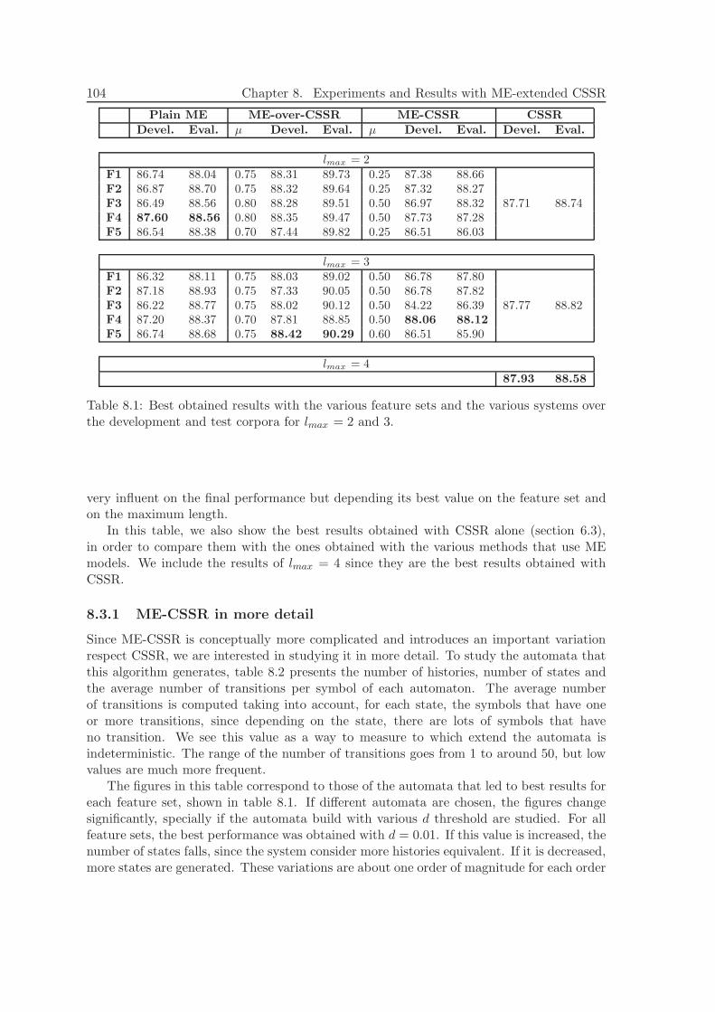
104 Chapter 8. Experiments and Results with ME-extended CSSR
Plain ME ME-over-CSSR ME-CSSR CSSR
Devel. Eval. µ Devel. Eval. µ Devel. Eval. Devel. Eval.
lmax = 2F1 86.74 88.04 0.75 88.31 89.73 0.25 87.38 88.66
87.71 88.74F2 86.87 88.70 0.75 88.32 89.64 0.25 87.32 88.27F3 86.49 88.56 0.80 88.28 89.51 0.50 86.97 88.32F4 87.60 88.56 0.80 88.35 89.47 0.50 87.73 87.28F5 86.54 88.38 0.70 87.44 89.82 0.25 86.51 86.03
lmax = 3F1 86.32 88.11 0.75 88.03 89.02 0.50 86.78 87.80
87.77 88.82F2 87.18 88.93 0.75 87.33 90.05 0.50 86.78 87.82F3 86.22 88.77 0.75 88.02 90.12 0.50 84.22 86.39F4 87.20 88.37 0.70 87.81 88.85 0.50 88.06 88.12
F5 86.74 88.68 0.75 88.42 90.29 0.60 86.51 85.90
lmax = 487.93 88.58
Table 8.1: Best obtained results with the various feature sets and the various systems overthe development and test corpora for lmax = 2 and 3.
very influent on the final performance but depending its best value on the feature set andon the maximum length.
In this table, we also show the best results obtained with CSSR alone (section 6.3),in order to compare them with the ones obtained with the various methods that use MEmodels. We include the results of lmax = 4 since they are the best results obtained withCSSR.
8.3.1 ME-CSSR in more detail
Since ME-CSSR is conceptually more complicated and introduces an important variationrespect CSSR, we are interested in studying it in more detail. To study the automata thatthis algorithm generates, table 8.2 presents the number of histories, number of states andthe average number of transitions per symbol of each automaton. The average numberof transitions is computed taking into account, for each state, the symbols that have oneor more transitions, since depending on the state, there are lots of symbols that haveno transition. We see this value as a way to measure to which extend the automata isindeterministic. The range of the number of transitions goes from 1 to around 50, but lowvalues are much more frequent.
The figures in this table correspond to those of the automata that led to best results foreach feature set, shown in table 8.1. If different automata are chosen, the figures changesignificantly, specially if the automata build with various d threshold are studied. For allfeature sets, the best performance was obtained with d = 0.01. If this value is increased, thenumber of states falls, since the system consider more histories equivalent. If it is decreased,more states are generated. These variations are about one order of magnitude for each order
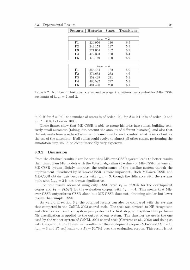
8.3. Experimental Results 105
Features Histories States Transitions
lmax = 2F1 220,956 110 6.5F2 244,153 147 5.9F3 221,054 132 5.9F4 472,393 150 6.4F5 472,149 190 5.9
lmax = 3F1 355,454 162 5.0F2 374,632 232 4.6F3 358,499 211 5.1F4 483,582 247 5.3F5 481,498 280 5.1
Table 8.2: Number of histories, states and average transitions per symbol for ME-CSSRautomata of lmax = 2 and 3.
in d: if for d = 0.01 the number of states is of order 100, for d = 0.1 it is of order 10 andfor d = 0.001 of order 1000.
These figures show that ME-CSSR is able to group histories into states, building rela-tively small automata (taking into account the amount of different histories), and also thatthe automata have a reduced number of transitions for each symbol, what is important forthe use of the automata. If all states could evolve to almost all other states, performing theannotation step would be computationally very expensive.
8.3.2 Discussion
From the obtained results it can be seen that ME-over-CSSR system leads to better resultsthan using plain ME models with the Viterbi algorithm (baseline) or ME-CSSR. In general,ME-CSSR system slightly improves the performance of the baseline system though theimprovement introduced by ME-over-CSSR is more important. Both ME-over-CSSR andME-CSSR obtain their best results with lmax = 3, though the difference with the systemsbuilt with lmax = 2 is not always significative.
The best results obtained using only CSSR were F1 = 87.93% for the developmentcorpus and F1 = 88.58% for the evaluation corpus, with lmax = 4. This means that ME-over-CSSR outperforms CSSR alone but ME-CSSR does not, obtaining similar but lowerresults than simple CSSR.
As we did in section 6.3, the obtained results can also be compared with the systemsthat competed in the CoNLL-2002 shared task. The task was devoted to NE recognitionand classification, and our system just performs the first step, so a system that performsNE classification is applied to the output of our system. The classifier we use is the oneused by the winner system of CoNLL-2002 shared task (Carreras et al., 2002) and doing sowith the system that obtains best results over the development corpus (ME-over-CSSR withlmax = 3 and F5 set) leads to a F1 = 76.79% over the evaluation corpus. This result is not
106 Chapter 8. Experiments and Results with ME-extended CSSR
significantly different from the system that classified 4th (Wu et al., 2002), that reportedF1 = 76, 61% for the evaluation corpus.
8.4 Conclusions of this Chapter
In this chapter, we have presented the obtained results when applying the methods thatcombine ME and CSSR to NER task. Also a baseline has been tested. Summarizing,we can say that, from the two presented systems, ME-over-CSSR is much simpler andleads to better results than ME-CSSR and the baseline. The second system, ME-CSSR,theoretically more sophisticated, improves slightly the baseline results but is always behindME-over-CSSR.
The main interest of developing these systems that combine ME and CSSR was toimprove the results obtained with CSSR alone. This goal is fulfilled only by ME-over-CSSRin which case the improvement is significant and the system can compete with the 4thsystem of CoNLL-2002 shared task.
We consider that the obtained results with ME-over-CSSR system are very interesting,since this method improves the CSSR performance combining it with simple ME models.In this way, we developed a fast and simple system that performs competitive NER takingadvantage of the CSSR ability to build minimal automata and of the ME capacity tocompute probability distributions taking into account many features.
Nevertheless, the fact that ME-CSSR obtains lower results than ME-over-CSSR andonly improves the baseline slightly is quite surprising, since it was expected that, being amore informed system that combines the power of ME models and CSSR, the results wouldbe better. This limited performance can be due to the fact that the amount of availabledata is not enough for CSSR to build correct automata, even if we are using a good methodfor sparse data such as ME models.
In this line, a point requesting further study is the trade-off between the data-sparsenesscaused by the fact of viewing histories as feature sets. Since the richer feature set we use,the less occurrences we will have of each particular history, the CSSR algorithm will haveless evidence to accurately build the causal states. On the other hand, richer feature setsshould produce better ME models, which can compensate this lack of evidence.
CHAPTER 9
Conclusions and Future Directions
To conclude, in this chapter we summarize the main contributions of this dissertation aswell as the publications related to them. Also, we state some future research lines that canfollow this work.
9.1 Summary and Conclusions
In this thesis, we have presented the application of a finite automata acquisition algorithmto some NLP tasks. This algorithm (CSSR) builds the causal state machine of a processfrom sequential data. This kind of machines have many interesting properties: they aredeterministic, markovian and are the minimal representation of a process. In fact, theautomata built with CSSR have the form of Markov Models with several suffixes groupedinto each state, building a much smaller automaton than a Markov Model for a givenprocess.
In order to use this algorithm for NLP tasks, first of all we have studied a variety ofaspects regarding the algorithm and its behavior when learning sentence patterns. Secondly,we have exposed an approach to introduce hidden information into the algorithm and thenapply it to NER in general and medical domain and Chunking. Finally, and consideringthe limitations that this approach has, we have proposed a method to combine CSSR withME models in order to build a system that takes into account more information.
9.1.1 Main Contributions
In the following points we summarize the contributions of this work, which we differentiatein three main lines:
1. Study of the ability of CSSR to capture text patterns.
We have performed some preliminary experiments in order to study the algorithm be-havior and its dependency on the various parameters. In this step, we have focused onthe study of the learned automata when the input for the system are data drawn from
107
108 Chapter 9. Conclusions and Future Directions
natural language texts, were some features have been highlighted. These automataare expected to reproduce the patterns of a text in terms of the selected features.First of all we have selected features related to Named Entities, in order to see howCSSR represents a text with this kind of entities, and secondly we have studied theability of the algorithm to capture the patterns of Noun Phrases in terms of the PoStags of each word.
These experiments have shown that CSSR is able to learn correctly these kind ofpatterns, though its performance is very dependent on the amount of available data.
2. Applying CSSR to NLP annotation tasks.
We have proposed an approach to introduce the hidden information, necessary for theannotation tasks, into the alphabet used by the algorithm. Then, these informationis taken into account when the automaton is built and can be afterwards used toannotate new text using a Viterbi algorithm. The main advantage of this techniquein comparison, for example, with a Markov Model is that the automata involved aremuch smaller so it is faster to annotate new text. Also, models with longer suffixes canbe built if enough data is available since the number of generated states will be muchsmaller than the equivalent Markov Model and thus more computationally tractable.
There are three main contributions our research introduces in the field of applyingCSSR to annotation task:
(a) The idea of introducing the hidden tags into the visible alphabet, building acomplete alphabet and performing a Viterbi algorithm to use the automaton toannotate new sentences.
(b) Two methods for dealing with unseen transitions have been presented. As weare performing annotation tasks with CSSR automata, there can be suffixesappearing in the test corpus that have not been seen in the training corpus.Then, some method to deal with these unseen events has to be developed.
(c) We also have proposed and tested a modification of the algorithm in the way itdetermines recurrent states. This modification theoretically leads to a loose inthe generalization power of CSSR but suits better the approached NLP tasks.
With these different proposed methods to apply CSSR to NLP annotation tasks, weperformed several experiments:
(a) The method has been validated by applying it to learn sentence patterns from acorpus annotated with a simple hand-made automaton, and checking that CSSRis able to exactly reproduce its behavior. The results show that CSSR is able toannotate perfectly this corpus.
(b) This approach has been applied to NER, with a deep study of the influence ofthe various parameters of the algorithm and of some different proposed imple-mentations. It has been shown that CSSR can build automata that give prettygood results in this task.
(c) The system has been also applied to Biomedical Named Entity Recognition, usinga very simple approach. The obtained results are comparable to other state-of-the-art systems, though some post-processing techniques should be implementedto improve the performance of CSSR in this task.
9.1. Summary and Conclusions 109
(d) Finally, the proposed approach has been used for Chunking task. In this case,various automata must be built to annotate each different kind of chunk and thentheir predictions must be combined. We have proposed and tested two differentmethods for combining the various chunkers obtaining not as good results as forNER when compared to other systems, but still being comparable with state-of-the-art systems.
3. Combining CSSR and Maximum Entropy Models.
Once the proposed approach to use CSSR for NLP tasks has been tested in varioustasks, and seeing that to improve the performance of the system it is necessary tointroduce more information into it, we have proposed to combine CSSR algorithm withME models. The goal of this combination is to take advantage of the good propertiesof CSSR (for example the ability of building minimal automata that represent aprocess) but combine it with the power of ME models, that can compute probabilitydistributions taking into account lots of features, what CSSR can not do.
In this line, we have proposed two approaches to combine these two methods. Thesemethods have been tested in NER task and compared with a baseline that used onlyCSSR. The developed systems and the obtained results can be summarized as follows:
(a) First approach (ME-over-CSSR) combines CSSR and ME models only in theannotation step, using the automata built with normal CSSR and the ME pro-babilities to predict the most likely tag for each word in a sentence. The resultsobtained with this system are quite good, beating both the baseline that usesME models and the results obtained with CSSR alone. That means that thecombination of CSSR and ME models really makes a more informed system.
(b) The second approach (ME-CSSR) uses ME models both in the automaton build-ing step and in the annotation step. This is a more complex proposal, thatintroduces modifications into the algorithm with the goal of building directlymore informed automata rather than using the original CSSR automata in com-bination with ME models. Nevertheless, the obtained results are worse thanthose of ME-over-CSSR, and do not improve those of CSSR alone. Regardingthe baseline, ME-CSSR slightly outperforms it.
To conclude this dissertation, we can say that CSSR algorithm is a powerful algorithmthat can learn the patterns of sentences in terms of some selected features, capturing thebehavior of NPs or NEs. It also can be satisfactorily applied to NER task, both in generaland medical domain but obtains not so competitive results in Chunking task. CSSR per-forms better as smaller is the vocabulary, since to learn good automata with big alphabets,huge amount of data would be necessary.
In fact, this is one of the main limitations of the algorithm: it needs and importantamount of data to perform good statistics and this ties the possibility of improving itsperformance by taking into account more features and increasing the vocabulary size. Forthat reason we have devised two methods to combine CSSR with ME models obtaininggood results with the first one but not improving CSSR alone for the second one. Thisopens a door to continue the research in this line, since it has been seen that combining MEand CSSR leads to a better system that using only CSSR, but there are still many issuesto be studied.
110 Chapter 9. Conclusions and Future Directions
9.1.2 Related Publications
The work presented in this PhD thesis has been published in various conferences. Here wesummarize these publications:
Study of CSSR ability to Learn Language Patterns
• Padro, M., & Padro, L. (2007b). Studying CSSR Algorithm Applicability on NLPTasks. Procesamiento del Lenguaje Natural, 39, 89–96.
Applying CSSR to NLP Annotating Tasks
• Padro, M., & Padro, L. (2005a). Applying a Finite Automata Acquisition Algorithmto Named Entity Recognition. Proceedings of 5th International Workshop on Finite-State Methods and Natural Language Processing (FSMNLP’05). Helsinki, Finland.
• Padro, M., & Padro, L. (2005b). Approaching Sequential NLP Tasks with an Au-tomata Acquisition Algorithm. Proceedings of International Conference on RecentAdvances in NLP (RANLP’05). Bulgaria.
• Padro, M., & Padro, L. (2005c). A Named Entity Recognition System Based on aFinite Automata Acquisition Algorithm. Procesamiento del Lenguaje Natural, 35,319–326.
• Dowdall, J., Keller, B., Padro, L., & Padro, M. (2007). An Automata Based Approachto Biomedical Named Entity Identification. Annual Meeting of Proceedings of theAnnual Meeting of the ISMB BioLINK Special Interest Group on Text Data Mining.Vienna, Austria.
Extending CSSR algorithm with ME models
• Padro, M., & Padro, L. (2007a). ME-CSSR: an extension of CSSR using maximumentropy models. Proceedings of the 2007 Conference on Finite-State Methods for NLP(FSMNLP). Potsdam, Germany.
9.2. Future Work 111
9.2 Future Work
Further work that can be done following the work presented in this dissertation can bedivided in two main lines: the first one following the proposed approach to apply CSSRto NLP annotation tasks and the second one regarding the combination of CSSR and MEmodels. In both directions other applications can be developed and also there is still workto be done regarding the implementation of the system and the tunning of the parameters.In next sections we briefly present some relevant future lines following these two directions.
9.2.1 CSSR for annotation tasks
Modifications of the System
We propose to modify the use of CSSR to make it more similar to a Hidden Markov Model(HMM), rather than using it as a visible Markov Model as done so far. The idea is to definethe alphabet of CSSR as the possible hidden information, as an HMM does, and let CSSRlearn an automaton reproducing the patterns of this information. This automaton will besimilar to the hidden part of a HMM but with much less states. Once the automaton isbuilt, emission probabilities could be added to each state.
Note that this would be a way of building much small HMMs, so probably modelsinvolving longer histories than HMMS could be built. Nevertheless, for the kind of tasksapproached in this PhD, to build HMMs is not a good approach, since there are just threehidden tags and the states will have too few information.
Other Applications
One of the applications we are interested in using CSSR is PoS tagging. This task cannot be directly approached using the proposed method to combine the visible part of thealphabet with the hidden tags since the visible information usually used in this task arethe words in a sentence and using them as a visible alphabet would be impossible. Then,it should be approached using the system proposed in previous section.
In this case, the alphabet of CSSR would be built by the PoS tags and CSSR would learnan automata reproducing the patterns of these tags. Then, the possible emissions (that forthe case of PoS tagging are the words) for each state will be added and its probabilitiescomputed.
Another point requesting further study is the combination of CSSR with some post-processing techniques, specially for the case of Biomedical NER. Such techniques have beenused in other systems, leading to a significative improvement of the results.
9.2.2 CSSR combined with ME models
Modifications of the Systems
Some interesting points requesting further study to improve the systems that combine MEmodels and CSSR are:
1. The use of different lengths for different features. In this way, just the most relevantfeatures will be taken into account for higher maximum lengths, allowing the use oflonger lmax values without exploiting the number of considered histories, as happenswith the current implementation.
112 Chapter 9. Conclusions and Future Directions
2. The possibility of introducing features for future words into the feature set for bothME-over-CSSR and ME-CSSR. This can be done without problem for ME-over-CSSRsystem, since it uses the features independently of the histories of the automaton, butit has to be studied carefully for the case of ME-CSSR, where histories include thefeatures of last lmax words. This means that introducing features about future wordswill modify the concept of history a little bit, since the future features for one wordwill be past features for another word that can be in the same history. For that reasonthis possibility has to be studied carefully specially for ME-CSSR.
3. Regarding ME-CSSR, we are also interested on studying why the performance islower than what we expected (often close to the baseline) and looking for some waysto improve it.
4. To improve ME-CSSR performance, one possibility is to use ME models and CSSRtogether to build a system more similar to a Hidden Markov Model, as it has beenproposed in section 9.2.1, but for tasks with B-I-O tags. The idea that we proposeis to set the vocabulary to the three hidden tags Σ = {B, I,O}. This would be atoo poor vocabulary for original CSSR, but since ME-CSSR builds states taking intoaccount all the features that we want to encode independently of the alphabet, thefinal automata could be rich enough. Thus, the automaton will have sets of historiesthat would build the states, the transition between states labeled by a B-I-O tag anda visible part that would be the visible part of the alphabet. This is a modification ofthe proposed ME-CSSR that separates the visible part of the alphabet and the hiddentags, and we think that it could be useful in the learning step since the vocabularysize (the classes of the ME model) will be much smaller so the estimated probabilitiesbetter.
Other Applications
For the case of the two systems that combine ME models and CSSR, the same applicationsto NLP task proposed with the original CSSR can be approached. In this way, the systemscould be applied to tasks such as Biomedical NER and Chunking since CSSR led to rea-sonably good results but needed more information to improve them, or to PoS tagging asexplained in previous section. It would be interesting to see if, as for NER, the system thatuses ME models is better than the one that uses only CSSR.
Also, since combining CSSR with ME models allows us to introduce more informationinto the system, it could be applied to more complex tasks such as NE classification bothin general and Biomedical domains, what can not be done with original CSSR because ofthe limitation in the alphabet size.
Bibliography
Aberdeen, J., Burger, J. D., Day, D., Hirschman, L., Robinson, P., & ain, M. V. (1995).mitre: Description of the alembic system used for MUC-6, 141–155. Proceedings of the6th Messsage Understanding Conference, MUC-6. Columbia, Maryland: Morgan Kauf-mann Publishers, Inc.
Abney, S. (1991). Parsing by chunks. R. Berwick, S. Abney and C. Tenny (eds.) Principle–based Parsing. Dordrecht: Kluwer Academic Publishers.
Alfonseca, E., & Manandhar, S. (2002). An unsupervised method for general named en-tity recognition and automated concept discovery. Proceedings of the first InternationalConference of Global WordNet Association. Mysore, India.
Ando, R. K., & Zhang, T. (2005). A high-performance semi-supervised learning method fortext chunking. ACL ’05: Proceedings of the 43rd Annual Meeting on Association for Com-putational Linguistics (pp. 1–9). Morristown, NJ, USA: Association for ComputationalLinguistics.
Aone, C., Halverson, L., Hampton, T., & Ramos-Santacruz, M. (1998). SRA: Description ofthe IE2 system used for MUC. Proceedings of the 7th Messsage Understanding Conference,MUC-7. Fairfax, Virginia.
Appelt, D. E., Hobbs, J. R., Bear, J., Israel, D., Kameyama, M., Kehler, A., Martin, D.,Myers, K., & Tyson, M. (1995). SRI international fastus system muc-6 test results andanalysis, 237–248. Proceedings of the 6th Messsage Understanding Conference. Columbia,Maryland: Morgan Kaufmann Publishers, Inc.
Asahara, M., & Matsumoto, Y. (2003). Japanese named entity extraction with redundantmorphological analysis. Proceedings of the 2003 Conference of the North American Chap-ter of the Association for Computational Linguistics on Human Language Technology,NAACL ’03 (pp. 8–15). Morristown, NJ, USA: Association for Computational Linguis-tics.
Atserias, J., Casas, B., Comelles, E., Gonzalez, M., Padro, L., & Padro, M. (2006). FreeLing1.3: Syntactic and semantic services in an open-source NLP library. Proceedings of the fifth
113
114 BIBLIOGRAPHY
international conference on Language Resources and Evaluation (LREC 2006). Genoa,Italy. http://www.lsi.upc.edu/ nlp/freeling.
Baker, J. (1979). Trainable grammars for speech recognition. Speech communication paperspresented at the 97th Meeting of the Acoustical Society (pp. 547–550).
Bender, O., Och, F. J., & Ney, H. (2003). Maximum entropy models for named entityrecognition. Proceedings of the seventh conference on Natural Language Learning atHLT-NAACL 2003, CoNLL-2003 (pp. 148–151). Morristown, NJ, USA: Association forComputational Linguistics.
Bengio, Y. (1996). Markovian models for sequential data. Technical Report 1049, Dept.IRO. Universite de Montreal.
Bengio, Y., & Frasconi, P. (1995). An input output HMM architecture. Advances in NeuralInformation Processing Systems (pp. 427–434). The MIT Press.
Berger, A., Pietra, S. D., & Pietra, V. D. (1996). A maximum entropy approach to naturallanguage processing. Computational Linguistics, 22, 39–71.
Bikel, D. M., Miller, S., Schwartz, R., & Weischedel, R. (1997). Nymble: A high performancelearning name-finder. Proceedings of the 5th Conference on Applied Natural LanguageProcessing, ANLP. Washington DC.
Black, W. J., Rinaldi, F., & Mowatt, D. (1998). Facile: Description of the ne system usedfor muc-7. Proceedings of the 7th Message Understanding Conference, MUC-7. Fairfax,Virginia.
Black, W. J., & Vasilakopoulos, A. (2002). Language-independent named entity classifica-tion by modified transformation-based learning and by decisi on tree induction. Proceed-ings of CoNLL-200 (pp. 159–162). Taipei, Taiwan.
Borthwick, A., Sterling, J., Agichtein, E., & Grishman, R. (1998). nyu: Description of themene named entity system as used in muc-7. Proceedings of the 7th Message Understand-ing Conference, MUC-7. Fairfax, Virginia.
Borthwick, A. E. (1999). A maximum entropy approach to named entity recognition. Doc-toral dissertation, New York University, New York, NY, USA. Adviser-Ralph Grishman.
Boschetti, F. (2007). Mapping the complexity of ecological models. Ecological Complexity,5, 37–47.
Bottou, L. (1991). Une approche theorique de l’apprentissage connexionniste: Applicationsa la reconnaissance de la parole. Doctoral dissertation, Universite de Paris XI, Orsay,France.
Brill, E. (1995). Transformation–based error–driven learning and natural language process-ing: A case study in part–of–speech tagging. Computational Linguistics, 21, 543–565.
Buchholz, S., Veenstra, J., & Daelemans, W. (1999). Cascaded grammatical relation as-signment. In Proceedings of EMNLP/VLC-99 (pp. 239–246). University of Maryland,USA.
BIBLIOGRAPHY 115
Budi, I., & Bressan, S. (2003). Association rules mining for name entity recognition. Proceed-ings of the Fourth International Conference on Web Information Systems Engineering,WISE ’03. Washington, DC, USA: IEEE Computer Society.
Buhlmann, P., & Wyner, A. J. (1999). Variable length markov chains. The Annals ofStatistics, 27 (pp. 480–513).
Burger, J. D., Henderson, J. C., & Morgan, W. T. (2002). Statistical named entity recognizeradaptation. Proceedings of CoNLL-2002 (pp. 163–166). Taipei, Taiwan.
Cabre, T., Condamines, A., & Sanjuan, F. I. (2005). Introduction: Application-driventerminology engineering. Terminology, 11, 1–20.
Carreras, X., Chao, I., Padro, L., & Padro, M. (2004). Freeling: An open-source suite of lan-guage analyzers. Proceedings of the 4th International Conference on Language Resourcesand Evaluation (LREC’04). Lisbon, Portugal.
Carreras, X., & Marquez, L. (2003). Phrase recognition by filtering and ranking withperceptrons. Proceedings of the International Conference on Recent Advances on NaturalLanguage Processing (RANLP’03). Borovets, Bulgaria.
Carreras, X., Marquez, L., & Padro, L. (2002). Named entity extraction using adaboost.Proceedings of CoNLL Shared Task (pp. 167–170). Taipei, Taiwan.
Carreras, X., Marquez, L., & Padro, L. (2003a). Learning a perceptron-based named en-tity chunker via online recognition feedback. CoNLL 2003 Shared Task Contribution.Edmonton, Canada.
Carreras, X., Marquez, L., & Padro, L. (2003b). A simple named entity extractor usingadaboost. CoNLL 2003 Shared Task Contribution. Edmonton, Canada.
Castellvı, M. T. C., Bagot, R. E., & Palatresi, J. V. (2001). Automatic term detection: Areview of current systems. In D. Bourigault, C. Jacquemin and M.-C. L’Homme (Eds.),Recent advances in computational terminology, 53–88. Amsterdam/Philadelphia: JohnBenjamins.
Charniak, E. (2000). Bllip 1987-89 wsj corpus release 1. Linguistic Data Consortium.Philadelphia.
Chieu, H. L., & Ng, H. T. (2002). Named entity recognition: A maximum entropy approachusing global information. COLING.
Chieu, H. L., & Ng, H. T. (2003). Named entity recognition with a maximum entropyapproach. Proceedings of the seventh conference on Natural language learning at HLT-NAACL 2003, CoNLL-2003 (pp. 160–163). Morristown, NJ, USA: Association for Com-putational Linguistics.
Chinchor, N. A. (1998). Overview of muc-7/met-2. Proceedings of the 7th Message Under-standing Conference,MUC-7. Fairfax, Virginia.
Chinchor, N. A., Robinson, P., & Brown, E. (1998). HUB-4 named entity task definition.Proceedings of the DARPA Broadcast News Workshop. Herndon, VA.
116 BIBLIOGRAPHY
Chung, T. M. (2003). A corpus comparison approach for terminology extraction. Termi-nology, 9, 221–246(26).
Church, K. W. (1988). A stochastic parts program and noun phrase parser for unrestrictedtext. Proceedings of the 1st Conference on Applied Natural Language Processing, ANLP(pp. 136–143).
Cimiano, P., & Volker, J. (2005). Towards large-scale, open-domain and ontology-basednamed entity classification. Proceedings of the International Conference on Recent Ad-vances in Natural Language Processing (RANLP’05) (pp. 166–172). Borovets, Bulgaria:INCOMA Ltd.
Clarke, R. W., Freeman, M. P., & Watkins, N. W. (2003). The application of computationalmechanics to the analysis of geomagnetic data. Physical Review E, 67, 016203.
Cointet, J.-P., Faure, E., & Roth, C. (2007). Intertemporal topic correlations in onlinemedia. Proc. ICWSM Intl Conf Weblogs Social Media. Boulder, CO, USA.
Collins, M. (2002). Ranking algorithms for named-entity extraction: boosting and the votedperceptron. Proceedings of the 40th Annual Meeting on Association for ComputationalLinguistics,ACL ’02 (pp. 489–496). Morristown, NJ, USA: Association for ComputationalLinguistics.
Collins, M., & Singer, Y. (1999). Unsupervised models for named entity classification.Proceedings of the Joint SIGDAT Conference on Empirical Methods in Natural LanguageProcessing and Very Large Corpora.
Crutchfield, J. P. (1994). The calculi of emergence: computation, dynamics and induc-tion. Proceedings of the NATO advanced research workshop and EGS topical workshopon Chaotic advection, tracer dynamics and turbulent dispersion (pp. 11–54). New York,NY, USA: Elsevier North-Holland, Inc.
Crutchfield, J. P., & Young, K. (1989). Inferring statistical complexity. Physical ReviewLetters, 63, 105–108.
Crutchfield, J. P., & Young, K. (1990). Computation at the onset of chaos. In Wojciech H.Zurek, editor, Complexity, Entropy, and the Physics of Information, volume 8 of SantaFe Institute Studies in the Sciences of Complexity, pages 223-269. Massachusetts.
Cucchiarelli, A., & Velardi, P. (2001). Unsupervised named entity recognition using syn-tactic and semantic contextual evidence. Computational Linguistics, 27, 123–131.
Cucerzan, S., & Yarowsky, D. (1999). Language independent named entity recognitioncombining morphological and contextual evidence. Proceedings of the 1999 Joint SIGDATConference on EMNLP and VLC (pp. 90–99).
Cucerzan, S., & Yarowsky, D. (2002). Language independent ner using a unified modelof internal and contextual evidence. Proceedings of CoNLL-2002 (pp. 171–174). Taipei,Taiwan.
BIBLIOGRAPHY 117
Cumby, C., & Roth, D. (2003). Feature extraction languages for propositionalized relationallearning. IJCAI’03 Workshop on Learning Statistical Models from Relational Data. Aca-pulco, Mexico.
Curran, J. R., & Clark, S. (2003). Language independent ner using a maximum entropy tag-ger. Proceedings of the seventh conference on Natural Language Learning at HLT-NAACL2003, CoNLL-2003 (pp. 164–167). Morristown, NJ, USA: Association for ComputationalLinguistics.
Darroch, J. N., & Ratcliff, D. (1972). Generalized iterative scaling for log-linear models.The Annals of Mathematical Statistics, 43, 1470–1480.
Daume III, H. (2004). Notes on CG and LM-BFGS optimization of logistic regression.Paper and implementation available at http://www.cs.utah.edu/~hal/megam/.
Dejean, H. (2000). Learning syntactic structures with xml. Proceedings of CoNLL-2000 andLLL-2000 (pp. 133–135). Lisbon, Portugal.
Della Pietra, S., Della Pietra, V. J., & Lafferty, J. D. (1997). Inducing features of randomfields. IEEE Transactions on Pattern Analysis and Machine Intelligence, 19, 380–393.
Dietterich, T. G. (2002). Machine learning for sequential data: A review. Proceedings ofthe Joint IAPR International Workshop on Structural, Syntactic, and Statistical PatternRecognition (pp. 15–30). London, UK: Springer-Verlag.
Doddington, G., Mitchell, A., Przybocki, M., Ramshaw, L., Strassel, S., & Weischedel, R.(2004). The Automatic Content Extraction (ACE) Program–Tasks, Data, and Evaluation.Proceedings of LREC 2004, 837–840.
Dowdall, J., Keller, B., Padro, L., & Padro, M. (2007). An automata based approach tobiomedical named entity identification. Annual Meeting of Proceedings of the AnnualMeeting of the ISMB BioLINK Special Interest Group on Text Data Mining. Vienna,Austria.
Etzioni, O., Cafarella, M., Downey, D., Popescu, A.-M., Shaked, T., Soderland, S., Weld,D. S., & Yates, A. (2005). Unsupervised named-entity extraction from the web: anexperimental study. Artificial Intelligence, 165, 91–134.
Evans, R. (2003). A framework for named entity recognition in the open domain. Proceedingsof Recent Advances in Natural Language Processing, RANLP’03 (pp. 137 – 144). Borovetz,Bulgaria.
Finkel, J., Dingare, S., Nguyen, H., Nissim, M., Sinclair, G., & Manning, C. (2004). Ex-ploiting context for biomedical entity recognition: From syntax to the web. Proceedings ofthe Joint Workshop on Natural Language Processing in Biomedicine and its Applications(JNLPBA).
Florian, R. (2002). Named entity recognition as a house of cards: Classifier stacking.Proceedings of CoNLL-2002 (pp. 175–178). Taipei, Taiwan.
118 BIBLIOGRAPHY
Florian, R., Ittycheriah, A., Jing, H., & Zhang, T. (2003). Named entity recognition throughclassifier combination. Proceedings of the seventh conference on Natural language learningat HLT-NAACL 2003 (pp. 168–171). Morristown, NJ, USA: Association for Computa-tional Linguistics.
Galil, Z., & Giancarlo, R. (1988). Data structures and algorithms for approximate stringmatching. Complexity, 4, 33–72.
Garcia, P., Cano, A., & Ruiz, J. (2000). A comparative study of two algorithms for automataidentification. Proceedingf of the 5th International Colloquium on Grammatical Inference,ICGI 2000.
Garcia, P., Vidal, E., & Casacuberta, F. (1987). Local languages, the sucessor method,and a step towards a general methodology for the inference of regular grammars. IEEETransactions on Pattern Analysis and Machine Intelligence, PAMI, 9(6), 841–845.
Gold, E. M. (1978). Complexity of automaton identification from given data. Informationand Control, 37(3), 302–320.
Good, I. J. (1963). Maximum entropy for hypothesis formulation, especially for multidi-mensional contingency tables. Annals of Mathematical Statistics, 34, 911–934.
Grishman, R., & Sundheim, B. (1996). Message understanding conference-6: a brief history.Proceedings of the 16th conference on Computational linguistics (pp. 466–471). Morris-town, NJ, USA: Association for Computational Linguistics.
GuoDong, Z., & Jian, S. (2004). Exploring deep knowledge resources in biomedical namerecognition. COLING 2004 International Joint workshop on Natural Language Process-ing in Biomedicine and its Applications (NLPBA/BioNLP) 2004 (pp. 99–102). Geneva,Switzerland: COLING.
Hammerton, J. (2003). Named entity recognition with long short-term memory. Proceedingsof the seventh conference on Natural language learning at HLT-NAACL 2003, CoNLL-2003 (pp. 172–175). Morristown, NJ, USA: Association for Computational Linguistics.
Hanson, J. E. (1993). Computational mechanics of cellular automata. Doctoral dissertation,University of California, Berkeley.
Hendrickx, I., & van den Bosch, A. (2003). Memory-based one-step named-entity recogni-tion: effects of seed list features, classifier stacking, and unannotated data. Proceedings ofthe seventh conference on Natural language learning at HLT-NAACL 2003 (pp. 176–179).Morristown, NJ, USA: Association for Computational Linguistics.
Holmes, M. P., & Isbell, C. L. (2006). Looping suffix tree-based inference of partiallyobservable hidden state. ICML ’06: Proceedings of the 23rd international conference onMachine learning (pp. 409–416). New York, NY, USA: ACM Press.
Humphreys, K., Gaizauskas, R., Huyck, C., Mitchell, B., Cunningham, H., & Wilks, Y.(1998). University of Sheffield: Description of the LaSIE-II system and used for MUC-7.Proc. MUC-7.
BIBLIOGRAPHY 119
Jacquemin, C., & Bourigault, D. (2003). Term extraction and automatic indexing. InR. Mitkov (Ed.), Handbook of computational linguistics, 599–615. Oxford.
Jansche, M. (2002). Named entity extraction with conditional markov models and classifiers.Proceedings of CoNLL-2002 (pp. 179–182). Taipei, Taiwan.
Jaynes, E. T. (1957). Information theory and statistical mechanics. Physical Review, 106,620–630.
Jelinek, F. (1990). Self-organized language modeling for speech recognition. In A. Waibeland K.-F. Lee (Eds.), Readings in speech recognition, 450–506. San Francisco, CA, USA:Morgan Kaufmann Publishers Inc.
Ji, H., & Grishman, R. (2006). Data selection in semi-supervised learning for name tagging.Proceedings of the Workshop on Information Extraction Beyond The Document in ACL’06(pp. 48–55). Sydney, Australia: Association for Computational Linguistics.
Johansson, C. (2000). A context sensitive maximum likelihood approach to chunking. Pro-ceedings of CoNLL-2000 and LLL-2000 (pp. 136–138). Lisbon, Portugal.
Kemeny, J. G., & Snell, J. L. (1976). Finite markov chains. Undergraduate Texts inMathematics. New York: Springer. 2nd edition.
Kemeny, J. G., Snell, J. L., & Knapp, A. W. (1976). Denumerable markov chains. GraduateTexts in Mathematics. New York: Springer. 2nd edition.
Kim, J. D., Ohta, T., Tateisi, Y., & Tsujii, J. (2003). GENIA corpus a semanticallyannotated corpus for bio-textmining. BioInformatics, 19, i180–i182.
Kim, J. D., Ohta, T., Tsuruoka, Y., Tateisi, Y., & Collier, N. (2004). Introduction to thebio-entity recognition task at JNLPBA. Proceedings of the International Joint Workshopon Natural Language Processing in Biomedicine and its Applications (JNLPBA), Geneva,Switzerland (pp. 70–75). held in conjunction with COLING’2004.
Kim, J.-H., Kang, I.-H., & Choi, K.-S. (2002). Unsupervised named entity classificationmodels and their ensembles. Proceedings of the 19th international conference on Com-putational linguistics (pp. 1–7). Morristown, NJ, USA: Association for ComputationalLinguistics.
Klein, D., Smarr, J., Nguyen, H., & Manning, C. D. (2003). Named entity recognitionwith character-level models. Proceedings of the seventh conference on Natural languagelearning at HLT-NAACL 2003 (pp. 180–183). Morristown, NJ, USA: Association forComputational Linguistics.
Koeling, R. (2000). Chunking with maximum entropy models. Proceedings of CoNLL-2000and LLL-2000 (pp. 139–141). Lisbon, Portugal.
Krupka, G. R., & Hausman, K. (1998). Isoquest, inc.: Description of the netowlTM extractorsystem as used for muc-7. Proceedings of the 7th Message Understanding Conference,MUC-7. Fairfax, Virginia.
120 BIBLIOGRAPHY
Kudo, T., & Matsumoto, Y. (2000). Use of support vector learning for chunk identification.Proceedings of CoNLL-2000 and LLL-2000 (pp. 142–144). Lisbon, Portugal.
Kudo, T., & Matsumoto, Y. (2001). Chunking with support vector machines. Proceedingsof NAACL-2001.
Lafferty, J., McCallum, A., & Pereira, F. (2001). Conditional random fields: Probabilisticmodels for segmenting and labeling sequence data. Eighteenth International Conferenceon Machine Learning (ICML-2001) (pp. 282–289). San Francisco, CA, USA: MorganKaufmann Publishers Inc.
Lari, K., & Young, S. J. (1990). The estimation of stochastic context-gree grammars usingthe inside-outside algorithm. Computer Speech and Language, 4, 35–56.
Lari, K., & Young, S. J. (1991). Application of stochastic context-free grammars using theinside-outside algorithm. Computer Speech and Language, 5, 237–257.
Lauritzen, S. L. (1996). Graphical models. Oxford University Press.
Lee, K.-J., Hwang, Y.-S., Kim, S., & Rim, H.-C. (2004). Biomedical named entity recogni-tion using two-phase model based on svms. J. of Biomedical Informatics, 37, 436–447.
Lee, Y.-S., & Wu, Y.-C. (2007). A robust multilingual portable phrase chunking system.Expert Systems with Applications, 33, 590–599.
L’Homme, M.-C., Heid, U., & Sager, J. C. (2003). Terminology during the past decade(1994-2004). Terminology, 9, 151–161.
Li, H., Webster, J., & Kit, C. (2003a). Transductive hmm based chinese text chunking.Proceeding of International Conference on Natural Language Processing and KnowledgeEngineering (pp. 257–262).
Li, H., Zhu, J., & Yao, T. (2004). Svm based chinese text chunking. Journal of ChineseInformation Processing, 18, 1–7.
Li, S., Liu, Q., & Yang, Z. (2003b). Chunking based on maximum entropy. Chinese Journalof Computer, 25, 1734–1738.
Lin, J. (1991). Divergence measures based on the shannon entropy. IEEE Transactions onInformation Theory, 37, 145–151.
Lin, Y.-F., Tsai, T.-H., Chou, W.-C., Wu, K.-P., Sung, T.-Y., & Hsu, W.-L. (2004). Amaximum entropy approach to biomedical named entity recognition. BIOKDD (pp. 56–61).
Malouf, R. (2002a). A comparison of algorithms for maximum entropy parameter estima-tion. CoNLL-2002 (pp. 49–55). Taipei, Taiwan.
Malouf, R. (2002b). Markov models for language-independent named entity recognition.Proceedings of CoNLL-2002 (pp. 187–190). Taipei, Taiwan.
Manning, C. D., & Schutze, H. (1998). Foundations of statistical natural language process-ing. The MIT Press.
BIBLIOGRAPHY 121
Mansouri, A., Affendey, L. S., & Mamat, A. (2008a). Named entity recognition approaches.International Journal of Computer Science and Network Security, IJCSNS, 8, 339–344.
Mansouri, A., Affendey, L. S., & Mamat, A. (2008b). Named entity recognition using a newfuzzy support vector machine. International Journal of Computer Science and NetworkSecurity, IJCSNS, 8, 320–325.
Mayfield, J., McNamee, P., & Piatko, C. (2003). Named entity recognition using hun-dreds of thousands of features. Proceedings of the seventh conference on Natural languagelearning at HLT-NAACL 2003 (pp. 184–187). Morristown, NJ, USA: Association forComputational Linguistics.
McCallum, A. (1995a). Instance-based utile distinctions for reinforcement learning withhidden state. ICML (pp. 387–395).
McCallum, A. (1995b). Reinforcement learning with selective perception and hidden state.Doctoral dissertation, Department of Computer Science, University of Rochester.
McCallum, A., Freitag, D., & Pereira, F. (2000). Maximum entropy Markov models forinformation extraction and segmentation. Proc. 17th International Conf. on MachineLearning (pp. 591–598). Morgan Kaufmann, San Francisco, CA.
McCallum, A., & Li, W. (2003). Early results for named entity recognition with conditionalrandom fields, feature induction and web-enhanced lexicons. Proceedings of the seventhconference on Natural language learning at HLT-NAACL 2003, CoNLL-2003 (pp. 188–191). Morristown, NJ, USA: Association for Computational Linguistics.
McNamee, P., & Mayfield, J. (2002). Entity extraction without language-specific resources.Proceedings of CoNLL-2002 (pp. 183–186). Taipei, Taiwan.
Meulder, F. D., & Daelemans, W. (2003). Memory-based named entity recognition usingunannotated data. Proceedings of the seventh conference on Natural language learning atHLT-NAACL 2003 (pp. 208–211). Morristown, NJ, USA: Association for ComputationalLinguistics.
Mikheev, A., Grover, C., & Moens, M. (1998). Description of the ltg system used for muc-7.Proceedings of the 7th Message Understanding Conference, MUC-7. Fairfax, Virginia.
Mikheev, A., Moens, M., & Grover, C. (1999). Named entity recognition without gazetteers.Proceedings of the ninth conference on European chapter of the Association for Compu-tational Linguistics, EACL’99 (pp. 1–8). Morristown, NJ, USA: Association for Compu-tational Linguistics.
Munro, R., Ler, D., & Patrick, J. (2003). Meta-learning orthographic and contextual modelsfor language independent named entity recognition. Proceedings of the seventh confer-ence on Natural language learning at HLT-NAACL 2003, CoNLL-2003 (pp. 192–195).Morristown, NJ, USA: Association for Computational Linguistics.
Murphy, K. P. (1996). Passively learning finite automata. Technical Report 96-04-017.Santa Fe Institute.
122 BIBLIOGRAPHY
Nadas, A. (1984). Estimation of probabilities in the language model of the ibm speechrecognition system. IEEE Transactions on Acoustics, Speech and Signal Processing, 4,859–861.
Nadeau, D., & Sekine, S. (2007). A survey of named entity recognition and classification.Journal of Linguisticae Investigationes, 30.
Nakagawa, H., & Mori, T. (2003). Automatic term recognition based on statistics of com-pound nouns and their components. Terminology, 9, 201–219.
N.Prieto (1995). Aprendizaje de modelos semanticos para sistemas de comprension deldiscurso continuo. Doctoral dissertation, Universidad Politecnica de Valencia. Advisor:Dr. E.Vidal.
Oncina, J. M., & Garcia, P. (1991). Inferring regular languages in polynomial update time.Pattern Recognition and Image Analysis, volume 1 of Series in Machine Perception andArtificial Intelligence (pp. 49–61). World Scientific.
Osborne, M. (2000). Shallow parsing as part-of-speech tagging. Proceedings of CoNLL-2000and LLL-2000 (pp. 145–147). Lisbon, Portugal.
Padro, M., & Padro, L. (2005a). Applying a finite automata acquisition algorithm to namedentity recognition. Proceedings of 5th International Workshop on Finite-State Methodsand Natural Language Processing (FSMNLP’05). Helsinki, Finland.
Padro, M., & Padro, L. (2005b). Approaching sequential NLP tasks with an automataacquisition algorithm. Proceedings of International Conference on Recent Advances inNLP (RANLP’05). Bulgaria.
Padro, M., & Padro, L. (2005c). A named entity recognition system based on a finiteautomata acquisition algorithm. Procesamiento del Lenguaje Natural, 35, 319–326.
Padro, M., & Padro, L. (2007a). ME-CSSR: an extension of CSSR using maximum entropymodels. Proceedings of the 2007 Conference on Finite-State Methods for NLP (FSMNLP).Potsdam, Germany.
Padro, M., & Padro, L. (2007b). Studying CSSR algorithm applicability on NLP tasks.Procesamiento del Lenguaje Natural, 39, 89–96.
Park, J., won Lee, J., Jo, H.-H., Yang, J.-S., & Moon, H.-T. (2006). Complexity and entropydensity analysis of the korean stock market. JCIS.
Park, S.-B., & Zhang, B.-T. (2003). Text chunking by combining hand-crafted rules andmemory-based learning. Proceedings of the 41st Annual Meeting on Association for Com-putational Linguistics, ACL’03 (pp. 497–504). Morristown, NJ, USA: Association forComputational Linguistics.
Patrick, J., Whitelaw, C., & Munro, R. (2002). Slinerc: The sydney language-independentnamed entity recogniser and classifier. Proceedings of CoNLL-2002 (pp. 199–202). Taipei,Taiwan.
BIBLIOGRAPHY 123
Perry, N., & Binder, P. M. (1999). Finite statistical complexity for sofic systems. PhysicalReview E, 60, 459–463.
Pla, F. (2000). Etiquetado lexico y analisis sintactico superficial basado en modelos es-tadısticos. Doctoral dissertation, Departament de Sistemes Informatics i Computacio,Universitat Politecnica de Valencia.
Pla, F., Molina, A., & Prieto, N. (2000). Improving Chunking by means of Lexical-Contextual Information in Statistical Language Models. Proceedings of ConNLL–2000.Lisbon, Portugal.
Ponomareva, N., Pla, F., Molina, A., & Rosso, P. (2007a). Biomedical named entity recog-nition: A poor knowledge hmm-based approach. NLDB (pp. 382–387).
Ponomareva, N., Rosso, P., Pla, F., & Molina, A. (2007b). Conditional random fields vs.hidden markov models in a biomedical named entity recognition task. In Proceedings ofRANLP 2007. Borovets, Bulgaria.
Rabiner, L. R. (1990). A tutorial on hidden markov models and selected applications inspeech recognition. Readings in Speech Recognition (eds. A. Waibel, K. F. Lee). SanMateo, CA: Morgan Kaufmann Publishers, Inc.
Ramshaw, L., & Marcus, M. P. (1995). Text chunking using transformation-based learning.Proceedings of the Third ACL Workshop on Very Large Corpora.
Ratnaparkhi, A. (1996). A maximum entropy part–of–speech tagger. Proceedings of the 1stConference on Empirical Methods in Natural Language Processing, EMNLP.
Ratnaparkhi, A. (1997). A simple introduction to maximum entropy models for naturallanguage processing Technical Report 97-08. Institute for Research in Cognitive Science,University of Pennsylvania.
Rau, L. F. (1991). Extracting company names from text. Seventh IEEE Conference onArtificial Intelligence Applications (pp. 29–32).
Ray, A. (2004). Symbolic dynamic analysis of complex systems for anomaly detection.Signal Process., 84, 1115–1130.
Riloff, E., & Jones, R. (1999). Learning dictionaries for information extraction by multi-level bootstrapping. Proceedings of National Conference on Artificial Intelligence (pp.474–479).
Rinaldi, F., Dowdall, J., Schneider, G., & Persidis, A. (2004a). Answering questions inthe genomics domain. Proceedings of the ACL04 Workshop on Question Answering inRestricted Domains. Barcelona, Spain.
Rinaldi, F., Hess, M., Dowdall, J., Molla, D., & Schwitter, R. (2004b). Question answering interminology-rich technical domains. In M. T. Maybury (Ed.), New directions in questionanswering, 71–82. AAAI Press.
Rissanen, J. (1983). A universal data compression system. IEEE Transactions in Informa-tion Theory, IT-29:656-664.
124 BIBLIOGRAPHY
Ron, D., Singer, Y., & Tishby, N. (1994a). Learning probabilistic automata with variablememory length. Computational Learing Theory (pp. 35–46).
Ron, D., Singer, Y., & Tishby, N. (1994b). The power of amnesia. Advances in NeuralInformation Processing Systems (pp. 176–183). Morgan Kaufmann Publishers, Inc.
Rulot, H. (1992). Ecgi: Un algoritmo de inferencia gramatical basado en la correccion deerrores. Doctoral dissertation, Universitat de Valencia. Advisor(s): Dr. E. Vidal and Dr.F. Casacuberta.
Rulot, H., & Vidal, E. (1987). Modelling (sub)string-length based constraints through agrammatical inference method. In Pattern recognition theory and applications, 451–459.Springer-Verlag.
Sanjuan, E., Dowdall, J., Ibekwe-Sanjuan, F., & Rinaldi, F. (2005). A symbolic approachto automatic multiword term structuring. Computer Speech and Language, 19, 524–542.
Santos, D., Seco, N., Cardoso, N., & Vilela, R. (2006). HAREM: an Advanced NEREvaluation Contest for Portuguese. Proceedings of LREC’2006 (pp. 1986–1991). Genoa,Italy.
Schutze, H., & Singer, Y. (1994). Part-of-speech tagging using a variable memory markovmodel. Proceedings of ACL 32’nd.
Segarra, E. (1993). Una aproximacion inductiva a la comprension del discurso continuo.Doctoral dissertation, Universidad Politecnica de Valencia.
Sekine, S. (1998). Nyu: Description of the japanese ne system used for Met-2. Proceedingsof the 7th Message Understanding Conference, MUC-7.. Fairfax, Virginia.
Sekine, S., & Isahara, H. (2000). Irex: Ir and ie evaluation project in japanese. 2ndInternational Conference on Language Resources and Evaluation (LREC) 2000 (pp. 1475–1480).
Shalizi, C. R. (2001). Causal architecture, complexity, and self-organization in time seriesand cellular automata. Doctoral dissertation, University of Michigan.
Shalizi, C. R., & Crutchfield, J. P. (2001). Computational mechanics: pattern, predictionstrucutre and simplicity. Journal of Statistical Physics, 104, 817–879.
Shalizi, C. R., & Shalizi, K. L. (2004). Blind construction of optimal nonlinear recursivepredictors for discrete sequences. Uncertainty in Artificial Intelligence: Proceedings ofthe Twentieth Conference.
Shalizi, C. R., Shalizi, K. L., & Crutchfield, J. P. (2002). An algorithm for pattern discoveryin time series. SFI Working Paper 02-10-060.
Shalizi, C. R., Shalizi, K. L., & Haslinger, R. (2004). Quantifying self-organization withoptimal predictors. Physical Review Letters, 93.
Shinyama, Y., & Sekine, S. (2004). Named entity discovery using comparable news articles.Proceedings of the 20th international conference on Computational Linguistics, COLING’04. Morristown, NJ, USA: Association for Computational Linguistics.
BIBLIOGRAPHY 125
Spasic, S., Ananiadou, S., McNaught, J., & Kumar, A. (2005). Text mining and ontologiesin biomedicine: Making sense of raw text. Briefings in Bioinformatics.
Stolcke, A., & Omohundro, S. (1993). Hidden markov model induction by bayesian modelmerging. In Stephen Jose Hanson, J. D. Gocwn, and C. Lee Giles, editors, Advances inNeural Information Processing Systems, volume 5, pages 11-18. Morgan Kaufmann, SanMateo, California.
Thollard, F., & Clark, A. (2002). Shallow parsing using probabilistic grammatical inference.ICGI ’02: Proceedings of the 6th International Colloquium on Grammatical Inference (pp.269–282). London, UK: Springer-Verlag.
Tino, P., & Dorner, G. (2001). Predicting the future of discrete sequences from fractalrepresentations of the past. Machine Learning, 45, 187–217.
Tjong Kim Sang, E. F. (2000). Text chunking by system combination. Proceedings ofCoNLL-2000 and LLL-2000 (pp. 151–153). Lisbon, Portugal.
Tjong Kim Sang, E. F. (2002a). Introduction to the conll-2002 shared task: Language-independent named entity recognition. Proceedings of CoNLL-2002 (pp. 155–158). Taipei,Taiwan.
Tjong Kim Sang, E. F. (2002b). Memory-based named entity recognition. Proceedings ofCoNLL-2002 (pp. 203–206). Taipei, Taiwan.
Tjong Kim Sang, E. F., & Buchholz, S. (2000). Introduction to the conll-2000 shared task:Chunking. Proceedings of CoNLL-2000 and LLL-2000 (pp. 127–132). Lisbon, Portugal.
Tjong Kim Sang, E. F., & De Meulder, F. (2003). Introduction to the conll-2003 sharedtask: Language-independent named entity recognition. Proceedings of CoNLL-2003 (pp.142–147). Edmonton, Canada.
Tjong Kim Sang, E. F., & Veenstra, J. (1999). Representing text chunks. Proceedings ofEACL’99 (pp. 173–179). Bergen, Norway.
Trakhtenbrot, B., & Barzdin, Y. (1973). Finite automata: Behaviour and synthesis. NorthHolland Publishing Company.
Tsukamoto, K., Mitsuishi, Y., & Sassano, M. (2002). Learning with multiple stacking fornamed entity recognition. Proceedings of CoNLL-2002 (pp. 191–194). Taipei, Taiwan.
Upper, D. R. (1997). Theory and algorithms for hidden markov models and generalizedhidden markov models. Doctoral dissertation, University of California at Berkeley.
van Halteren, H. (2000). Chunking with wpdv models. Proceedings of CoNLL-2000 andLLL-2000 (pp. 154–156). Lisbon, Portugal.
Varn, D. P., & Crutchfield, J. P. (2004). From finite to infinite range order via annealing:The causal architecture of deformation faulting in annealed close-packed crystals. PhysicsLetters A, 324, 299–307.
Veenstra, J. (1999). Memory-based text chunking. Nikos Fakotakis (ed), Machine learningin human language technology, workshop at ACAI 99. Chania, Greece.
126 BIBLIOGRAPHY
Veenstra, J., & van den Bosch, A. (2000). Single-classifier memory-based phrase chunking.Proceedings of CoNLL-2000 and LLL-2000 (pp. 157–159). Lisbon, Portugal.
Vidal, E., Thollard, F., C. de la Higuera, F. C., & Carrasco, R. (2005a). Probabilistic finite-state machines - part I. IEEE Transactions on Pattern Analysis and Machine Intelligence,27, 1013–1025.
Vidal, E., Thollard, F., C. de la Higuera, F. C., & Carrasco, R. (2005b). Probabilisticfinite-state machines - part II. IEEE Transactions on Pattern Analysis and MachineIntelligence, 27, 1025–1039.
Vilain, M., & Day, D. (2000). Phrase parsing with rule sequence processors: an applicationto the shared conll task. Proceedings of CoNLL-2000 and LLL-2000 (pp. 160–162). Lisbon,Portugal.
Wallach, H. M. (2004). Conditional random fields: An introduction (Technical ReportMS-CIS-04-21). Department of Computer and Information Science, University of Penn-sylvania.
Weeds, J., Dowdall, J., Schneider, G., Keller, B., & Weir, D. (2005). Using distributionalsimilarity to organise biomedical terminology. Terminology, 1, 107 – 141.
Weinberger, M. J., Lempel, A., & Ziv, J. (1992). A sequential algorithm for the universalcoding of finite memory sources. IEEE Transactions on Information Theory, 38, 1002–1014.
Weinberger, M. J., Rissanen, J., & Feder, M. (1995). A universal finite memory source.IEEE Transactions on Information Theory, 41, 643–652.
Weischedel, R. (1995). bbn: Description of the plum system as used for muc-6, 55–69. Pro-ceedings of the 6th Messsage Understanding Conference. Columbia, Maryland: MorganKaufmann Publishers, Inc.
Whitelaw, C., & Patrick, J. (2003). Evaluating corpora for named entity recognition usingcharacter-level features. Australian Conference on Artificial Intelligence (pp. 910–921).Springer.
Willems, F., Shtarkov, Y., & Tjalkens, T. (1995). The context-tree weighting method:basicproperties. IEEE Transactions in Information Theory, IT-41:653-664.
Wu, D., Ngai, G., & Carpuat, M. (2003). A stacked, voted, stacked model for namedentity recognition. Proceedings of the seventh conference on Natural language learning atHLT-NAACL 2003, CoNLL-2003 (pp. 200–203). Morristown, NJ, USA: Association forComputational Linguistics.
Wu, D., Ngai, G., Carpuat, M., Larsen, J., & Yang, Y. (2002). Boosting for named entityrecognition. Proceedings of CoNLL-2002 (pp. 195–198). Taipei, Taiwan.
Wu, Y.-C., Chang, C.-H., & Lee, Y.-S. (2006). A general and multi-lingual phrase chunkingmodel based on masking method. CICLing (pp. 144–155).
BIBLIOGRAPHY 127
Yu, S., Bai, S., & Wu, P. (1998). Description of the kent ridge digital labs system usedfor muc-7. Proceedings of the 7th Message Understanding Conference, MUC-7. Fairfax,Virginia.
Zhang, T., Damerau, F., & Johnson, D. (2001). Text chunking using regularized winnow.Meeting of the Association for Computational Linguistics (pp. 539–546).
Zhang, T., Damerau, F., & Johnson, D. (2002). Text chunking based on a generalization ofwinnow. J. Mach. Learn. Res., 2, 615–637.
Zhang, T., & Johnson, D. (2003). A robust risk minimization based named entity recog-nition system. Proceedings of the seventh conference on Natural language learning atHLT-NAACL 2003, CoNLL-2003 (pp. 204–207). Morristown, NJ, USA: Association forComputational Linguistics.
Zhou, G., & Su, J. (2002). Named entity recognition using an hmm-based chunk tagger. ACL’02: Proceedings of the 40th Annual Meeting on Association for Computational Linguistics(pp. 473–480). Morristown, NJ, USA: Association for Computational Linguistics.
Zhou, G., Su, J., & Tey, T. (2000). Hybrid text chunking. Proceedings of CoNLL-2000 andLLL-2000 (pp. 163–166). Lisbon, Portugal.