A 2 Model of the Flow in Hydrocyclones - COMSOL

September 17 - 19

A 2 Model of the Flow in Hydrocyclones

B. Chinè1, F. Concha2 and M. Meneses3

1 Escuela de Ciencia e Ing. Materiales, Instituto Tecnológico de Costa Rica, Cartago, Costa Rica; 2 Departamento de Ing. Metalúrgica, Universidad de Concepción, Concepción, Chile;

3 Escuela de Ing. en Producción Industrial, Instituto Tecnológico de Costa Rica, Cartago,Costa Rica

[email protected]

218/11/2014COMSOL CONFERENCE 2014 CAMBRIDGE

Presentation overview

• Introduction

• Swirling flows in hydrocyclones

• Geometry and experimental values of the simulated flow

• Physical model and equations

• Numerical results

• Conclusions

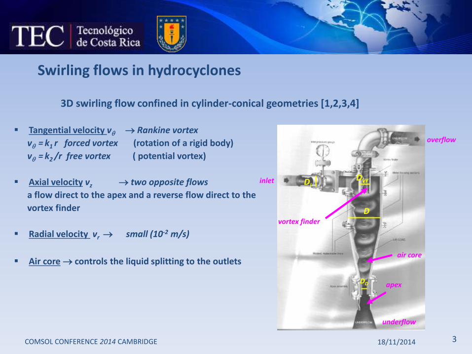
3D swirling flow confined in cylinder-conical geometries [1,2,3,4]

Tangential velocity v Rankine vortex

v = k1 r forced vortex (rotation of a rigid body)

v = k2 /r free vortex ( potential vortex)

Axial velocity vz two opposite flows

a flow direct to the apex and a reverse flow direct to the

vortex finder

Radial velocity vr small (10-2 m/s)

Air core controls the liquid splitting to the outlets


Swirling flows in hydrocyclones

vortex finder

apex

air core

D

DVF

DD

DIinlet

overflow

underflow


Swirling flows in hydrocyclones

From experimental works (LDV) we know that the flow in a hydrocyclone (conical and flat bottom) has the following properties:

velocity profiles of vz and v are not completely axisymmetric vz ,v , and their RMS values z and , only change their magnitude with pressure

p vz changes with z turbulence is neither homogeneous nor isotropic : z and are different and

depend on z and r the position of the air core does depend on p and the ratio DVF /DD (vortex finder

diameter/apex diameter)


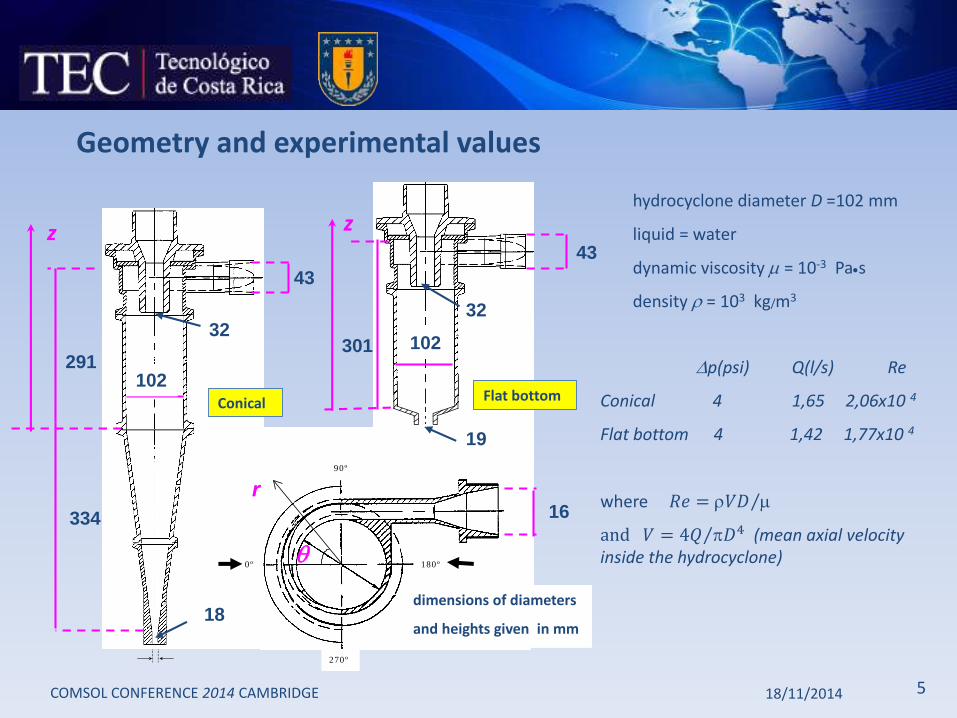
Geometry and experimental values

0º

90º

180º

270º

z

r

18

32

19

16

43

32

291

334

43

z

301

dimensions of diameters

and heights given in mm

p(psi) Q(l/s) Re

Conical 4 1,65 2,06x10 4

Flat bottom 4 1,42 1,77x10 4

where 𝑅𝑒 = 𝑉𝐷

and 𝑉 = 4𝑄 𝐷4 (mean axial velocity inside the hydrocyclone)

102

102

Conical Flat bottom

hydrocyclone diameter D =102 mm

liquid = water

dynamic viscosity = 10-3 Pas

density = 103 kg/m3


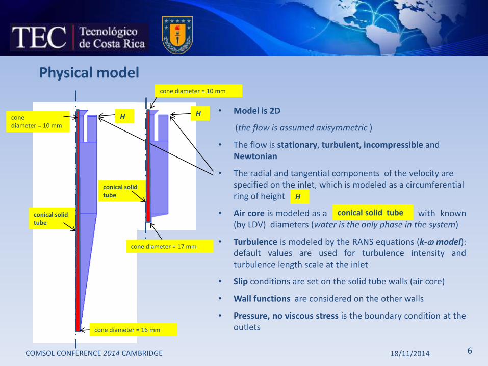
Physical model

• Model is 2D

(the flow is assumed axisymmetric )

• The flow is stationary, turbulent, incompressible andNewtonian

• The radial and tangential components of the velocity are specified on the inlet, which is modeled as a circumferential ring of height

• Air core is modeled as a with known(by LDV) diameters (water is the only phase in the system)

• Turbulence is modeled by the RANS equations (k- model):default values are used for turbulence intensity andturbulence length scale at the inlet

• Slip conditions are set on the solid tube walls (air core)

• Wall functions are considered on the other walls

• Pressure, no viscous stress is the boundary condition at theoutlets

H H

H

conical solidtube

conical solidtube

conical solid tube

cone diameter = 16 mm

conediameter = 10 mm




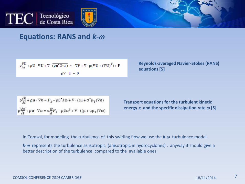
Equations: RANS and k-

Reynolds-averaged Navier-Stokes (RANS) equations [5]

Transport equations for the turbulent kinetic energy and the specific dissipation rate [5]

In Comsol, for modeling the turbulence of this swirling flow we use the k- turbulence model.

k- represents the turbulence as isotropic (anisotropic in hydrocyclones) : anyway it should give a better description of the turbulence compared to the available ones.


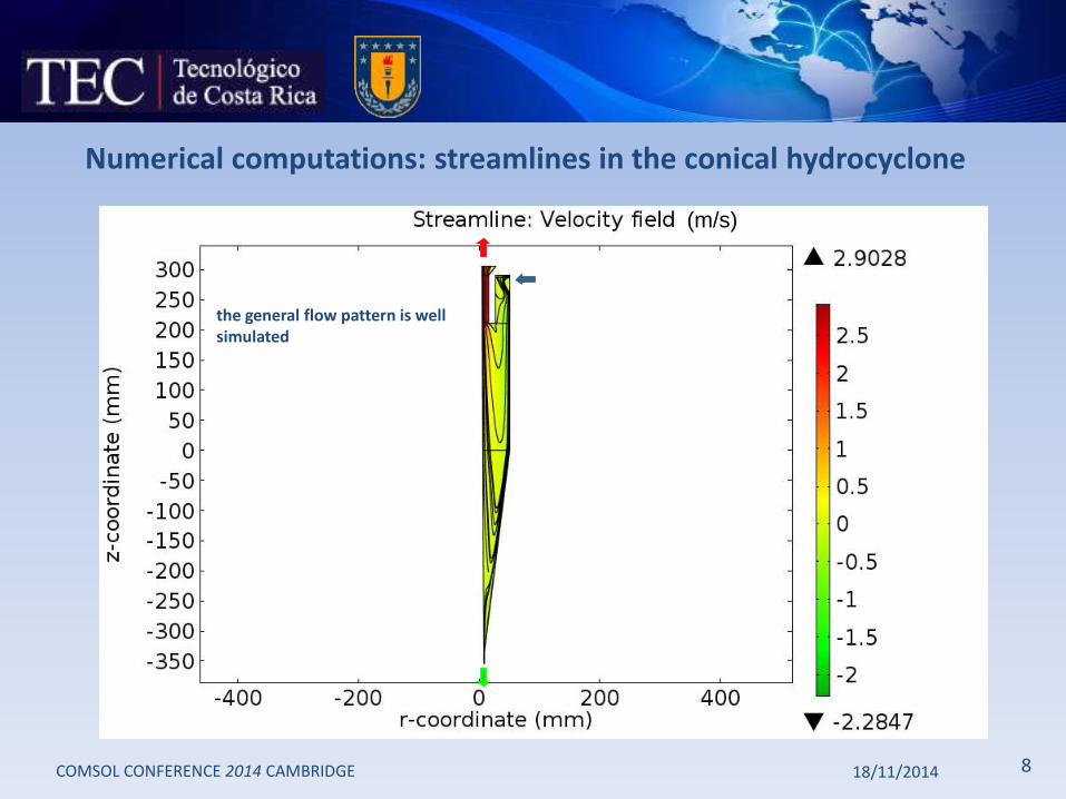
Numerical computations: streamlines in the conical hydrocyclone

(m/s)

the general flow pattern is well simulated


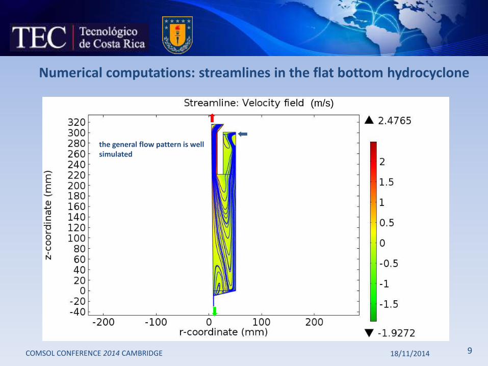
Numerical computations: streamlines in the flat bottom hydrocyclone

(m/s)

the general flow pattern is well simulated


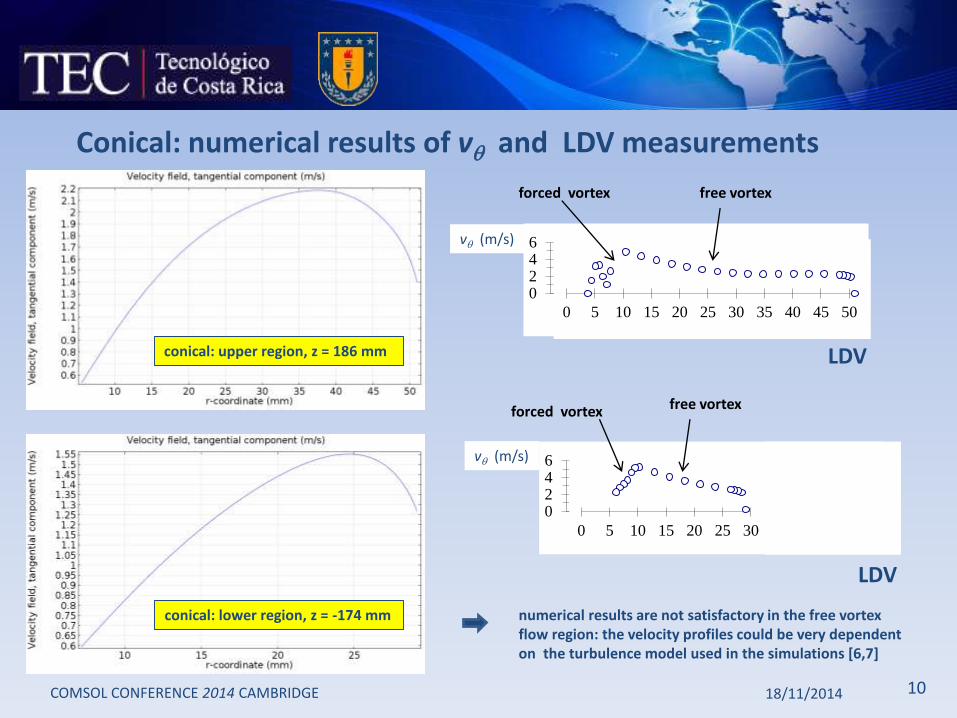
Conical: numerical results of v and LDV measurements

conical: upper region, z = 186 mm

conical: lower region, z = -174 mm

0246

051015202530354045500 5 10 15 20 25 30 35 40 45 50

v (m/s)

0246

051015202530354045500 5 10 15 20 25 30

v (m/s)

free vortexforced vortex

forced vortex free vortex

numerical results are not satisfactory in the free vortex flow region: the velocity profiles could be very dependent on the turbulence model used in the simulations [6,7]

LDV

LDV


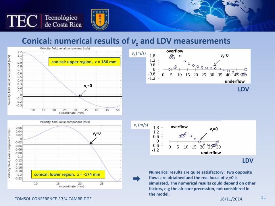
Conical: numerical results of vz and LDV measurements

conical: upper region, z = 186 mm

conical: lower region, z = -174 mm

-1.2-0.6

00.61.21.8

051015202530354045500 5 10 15 20 25 30 35 40 45 50

vz (m/s)

-1.2-0.6

00.61.21.8

051015202530354045500 5 10 15 20 25 30

vz (m/s)

underflow

overflow

overflow

underflow

Numerical results are quite satisfactory: two opposite flows are obtained and the real locus of vz=0 is simulated. The numerical results could depend on other factors, e.g the air core precession, not considered in the model.

vz=0

vz=0

vz=0

vz=0

LDV

LDV


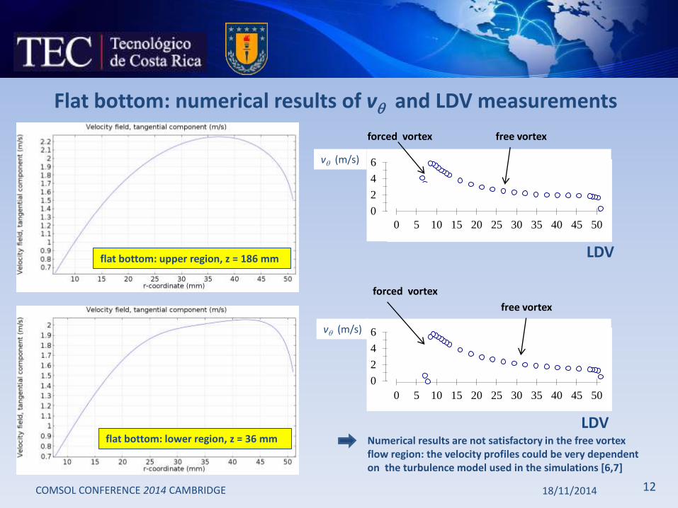
Flat bottom: numerical results of v and LDV measurements

flat bottom: upper region, z = 186 mm

flat bottom: lower region, z = 36 mm

0

2

4

6

051015202530354045500 5 10 15 20 25 30 35 40 45 50

v (m/s)

0

2

4

6

051015202530354045500 5 10 15 20 25 30 35 40 45 50

v (m/s)

LDV

LDV

forced vortex free vortex

forced vortex

free vortex

Numerical results are not satisfactory in the free vortex flow region: the velocity profiles could be very dependent on the turbulence model used in the simulations [6,7]


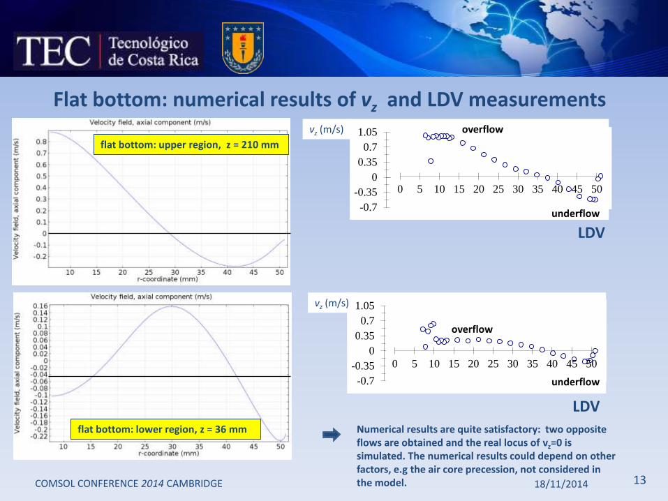
Flat bottom: numerical results of vz and LDV measurements

flat bottom: upper region, z = 210 mm

flat bottom: lower region, z = 36 mm

-0.7

-0.35

0

0.35

0.7

1.05

051015202530354045500 5 10 15 20 25 30 35 40 45 50

vz (m/s)

-0.7

-0.35

0

0.35

0.7

1.05

051015202530354045500 5 10 15 20 25 30 35 40 45 50

vz (m/s)

LDV

LDV

overflow

overflow

underflow

underflow

Numerical results are quite satisfactory: two opposite flows are obtained and the real locus of vz=0 is simulated. The numerical results could depend on other factors, e.g the air core precession, not considered in the model.


Conclusions

• Swirling flows in 2D hydrocyclones have been simulated by developing an axisymmetric model of the flow

• The general flow pattern is quite well reproduced

• Tangential velocity profiles differ from LDV measurements, they give a poor description of the free vortex: the k- turbulence model doesn't assume anisotropy , which is present in the flow

• Axial velocity profiles are quite satisfactory: some difference with LDV measurements could also be dependent on other factors, e.g. the air core precession , not considered here

• Although more complete models might be developed, e.g. 3D, including the modeling of the air core, the anisotropy of the turbulence, etc., computational requirements and computing times have to be considered.


References

[1] D.F. Kelsall , A study of the motion of solid particles in a hydraulic cyclone, Trans. Instn Chem. Engrs, 30 , 87-108 (1952).

[2] F. Concha, Flow pattern in hydrocyclones, KONA, 25, 97-132 (2007).[3] K.T. Hsieh and R.K Rajamani , Mathematical model of the hydrocyclone based on physics of fluid flow, AIChE

Journal 37(5), 735-746 (1991).[4] B. Chiné and F. Concha , Flow patterns in conical and cylindrical hydrocyclones, Chemical Engineering Journal,

80(1-3), 267-274 (2000).[5] Comsol AB, Comsol Multiphysics-CFD Module, User’s Guide, Version 4.3b (2013).[6] A. Davailles, E. Climent and F. Bourgeois, Fundamental understanding of swirling flow pattern in hydrocyclones,

Separation and Purification Technology, 92, 152-160 (2012).[7] Y. Rama Murthy and K. Udaya Bhaskar, Parametric CFD studies on hydrocyclone, Powder Technology, 230, 36-47

(2012).


Acknowledgements

Many thanks for your attention !

We would like to also acknowledge:

Vicerrectoría de Investigación y Extensión

Universidad de Concepción

… and to the organizers of the

Documents

A 2 Model of the Flow in Hydrocyclones - COMSOL