9.1 EstimatingDerivativeswithFiniteDiﬀerencesalgebra.sci.csueastbay.edu/~grewe/CS6825/Book_online/edgedetection.pdf · 1/256, 4/256 and 16/256 of the full range of brightness respectively

Chapter 9

EDGE DETECTION

9.1 Estimating Derivatives with Finite Differences

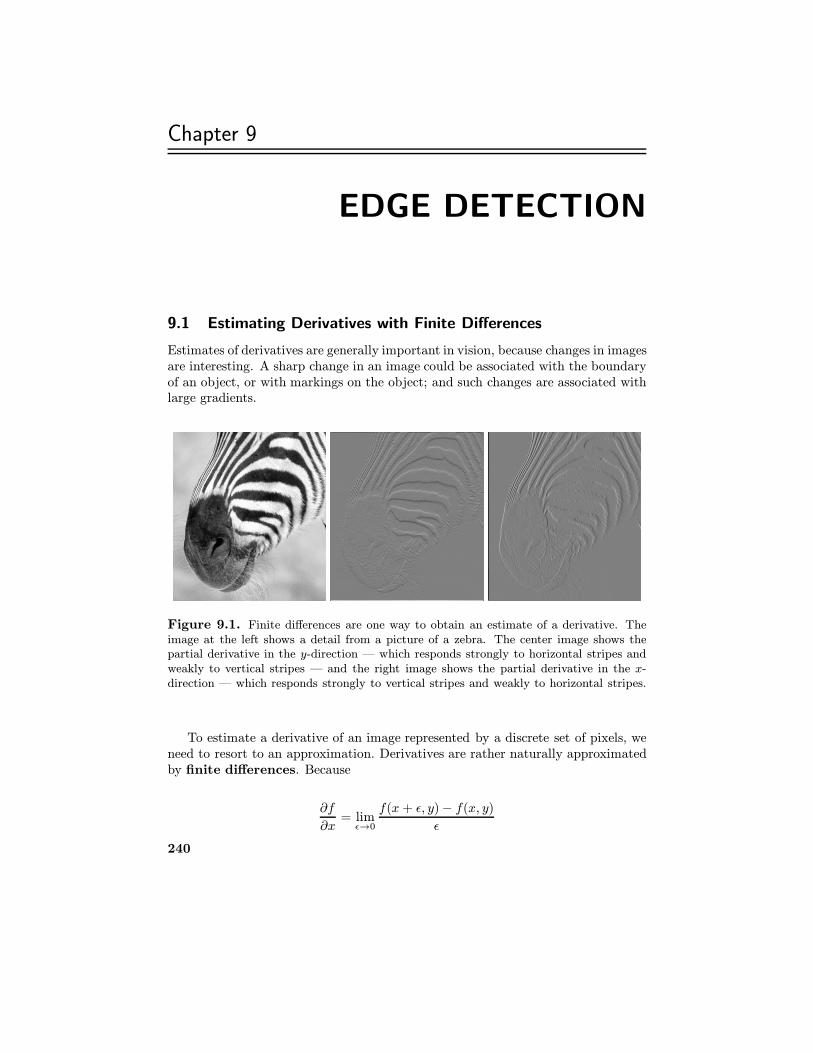
Estimates of derivatives are generally important in vision, because changes in imagesare interesting. A sharp change in an image could be associated with the boundaryof an object, or with markings on the object; and such changes are associated withlarge gradients.

Figure 9.1. Finite differences are one way to obtain an estimate of a derivative. Theimage at the left shows a detail from a picture of a zebra. The center image shows thepartial derivative in the y-direction — which responds strongly to horizontal stripes andweakly to vertical stripes — and the right image shows the partial derivative in the x-direction — which responds strongly to vertical stripes and weakly to horizontal stripes.

To estimate a derivative of an image represented by a discrete set of pixels, weneed to resort to an approximation. Derivatives are rather naturally approximatedby finite differences. Because

∂f

∂x= lim

ε→0

f(x + ε, y)− f(x, y)

ε

240

Section 9.1. Estimating Derivatives with Finite Differences 241

we might estimate a partial derivative as a symmetric difference:

∂h

∂x≈ hi+1,j − hi−1,j

This is the same as a convolution, where the convolution kernel is

G =

0 0 01 0 −10 0 0

Notice that this kernel could be interpreted as a template — it will give a largepositive response to an image configuration that is positive on one side and negativeon the other, and a large negative response to the mirror image.

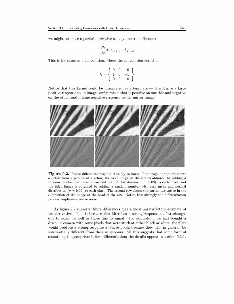
Figure 9.2. Finite differences respond strongly to noise. The image at top left showsa detail from a picture of a zebra; the next image in the row is obtained by adding arandom number with zero mean and normal distribution (σ = 0.03) to each pixel; andthe third image is obtained by adding a random number with zero mean and normaldistribution (σ = 0.09) to each pixel. The second row shows the partial derivative in thex-direction of the image at the head of the row. Notice how strongly the differentiationprocess emphasizes image noise.

As figure 9.2 suggests, finite differences give a most unsatisfactory estimate ofthe derivative. This is because this filter has a strong response to fast changesdue to noise, as well as those due to signal. For example, if we had bought adiscount camera with some pixels that were stuck at either black or white, the filterwould produce a strong response at those pixels because they will, in general, besubstantially different from their neighbours. All this suggests that some form ofsmoothing is appropriate before differentiation; the details appear in section 9.3.1.

242 Edge Detection Chapter 9

9.2 Noise

We have asserted that smoothing suppresses some kinds of noise. To be moreprecise we need a model of noise. Usually, by the term noise, we mean imagemeasurements from which we do not know how to extract information, or fromwhich we do not care to extract information; all the rest is signal. It is wrong tobelieve that noise does not contain information — for example, we should be ableto extract some estimate of the camera temperature by taking pictures in a darkroom with the lens-cap on. Furthermore, since we cannot say anything meaningfulabout noise without a noise model, it is wrong to say that noise is not modelled.Noise is everything we don’t wish to use, and that’s all there is to it.

9.2.1 Additive Stationary Gaussian Noise

In the additive stationary Gaussian noise model, each pixel has added to it avalue chosen independently from the same Gaussian probability distribution. Al-most always, the mean of this distribution is zero. The standard deviation is aparameter of the model. The model is intended to describe thermal noise in cam-eras.

Linear Filter Response to Additive Gaussian Noise

Assume we have a discrete linear filter whose kernel is G, and we apply it to a noiseimageN consisting of stationary additive Gaussian noise with mean µ and standarddeviation σ. The response of the filter at some point i, j will be:

R(N )i,j =∑u,v

Gi−u,j−vNu,v

Because the noise is stationary, the expectations that we compute will not de-pend on the point, and we assume that i and j are zero, and dispense with thesubscript. Assume the kernel has finite support, so that only some subset of thenoise variables contributes to the expectation; write this subset as n0,0, . . . , nr,s.The expected value of this response must be:

E[R(N )] =

∫ ∞−∞{R(N )}p(N0,0, . . . , Nr,s)dN0,0 . . . dNr,s

=∑u,v

G−u,−v{

∫ ∞−∞Nu,vp(Nu,v)dNu,v}

where we have done some aggressive moving around of variables, and integratedout all the variables that do not appear in each expression in the sum. Since all theNu,v are independent identically distributed Gaussian random variables with meanµ, we have that:

E[R(N )] = µ∑u,v

Gi−u,j−v

Section 9.2. Noise 243

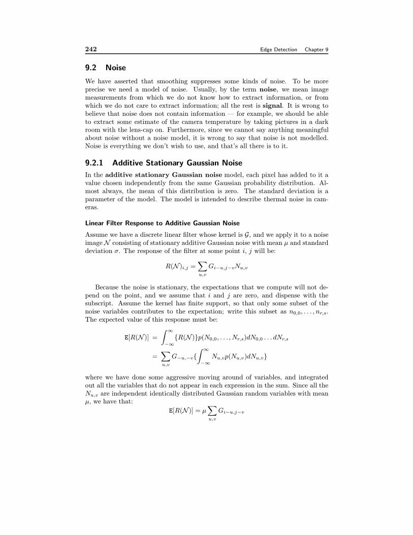
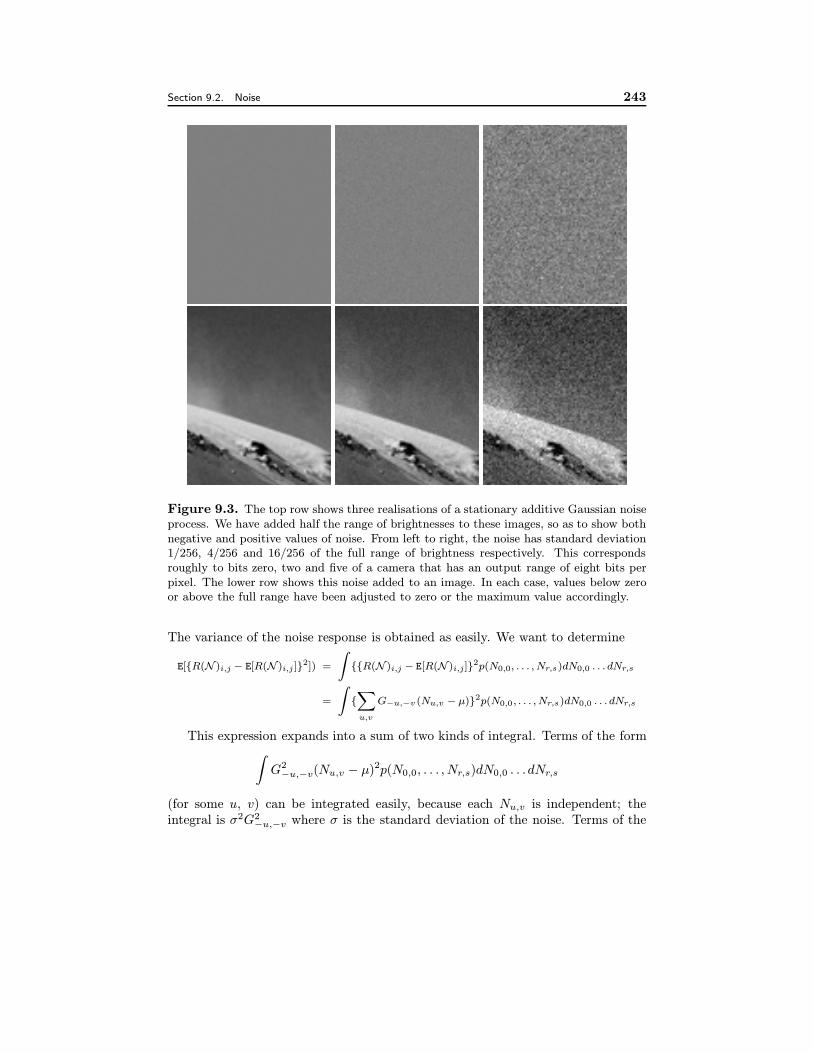
Figure 9.3. The top row shows three realisations of a stationary additive Gaussian noiseprocess. We have added half the range of brightnesses to these images, so as to show bothnegative and positive values of noise. From left to right, the noise has standard deviation1/256, 4/256 and 16/256 of the full range of brightness respectively. This correspondsroughly to bits zero, two and five of a camera that has an output range of eight bits perpixel. The lower row shows this noise added to an image. In each case, values below zeroor above the full range have been adjusted to zero or the maximum value accordingly.

The variance of the noise response is obtained as easily. We want to determine

E[{R(N )i,j − E[R(N )i,j ]}2]) =

∫{{R(N )i,j − E[R(N )i,j]}

2p(N0,0, . . . , Nr,s)dN0,0 . . . dNr,s

=

∫{∑u,v

G−u,−v (Nu,v − µ)}2p(N0,0, . . . , Nr,s)dN0,0 . . . dNr,s

This expression expands into a sum of two kinds of integral. Terms of the form∫G2−u,−v(Nu,v − µ)

2p(N0,0, . . . , Nr,s)dN0,0 . . . dNr,s

(for some u, v) can be integrated easily, because each Nu,v is independent; theintegral is σ2G2

−u,−v where σ is the standard deviation of the noise. Terms of the


form ∫G−u,−vG−a,−b(Nu,v − µ)(Na,b − µ)p(N0,0, . . . , Nr,s)dN0,0 . . . dNr,s

(for some u, v and a, b) integrate to zero, again because each noise term is inde-pendent. We now have:

E[{R(N )i,j − E[R(N )i,j]}2] = σ2

∑G2u,v

Finite Difference Filters and Gaussian Noise

From these results, we get some insight into the noise behaviour of finite differences.Assume we have an image of stationary Gaussian noise of zero mean, and considerthe variance of the response to a finite difference filter that estimates derivatives ofincreasing order. We shall use the kernel

0 01 −10 0

to estimate the first derivative. Now a second derivative is simply a first derivativeapplied to a first derivative, so the kernel will be:

0 0 01 −2 10 0 0

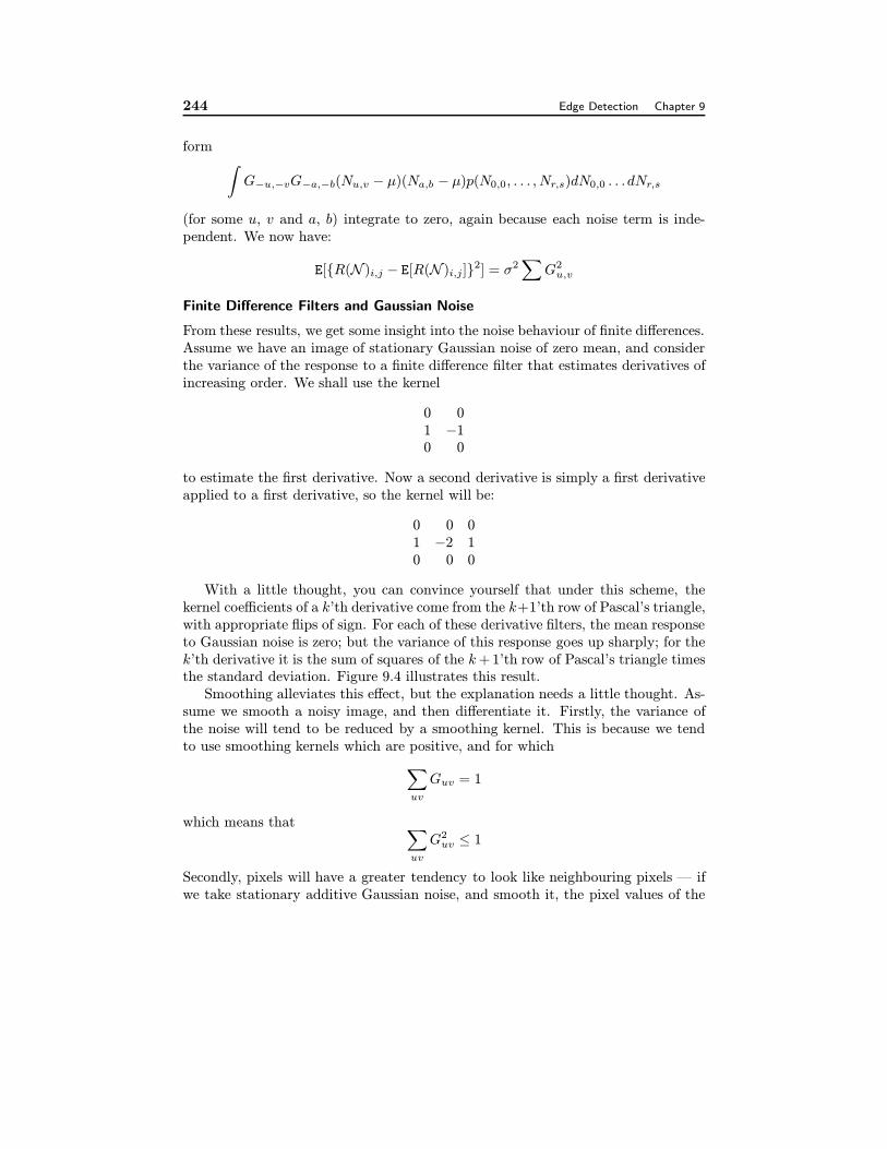
With a little thought, you can convince yourself that under this scheme, thekernel coefficients of a k’th derivative come from the k+1’th row of Pascal’s triangle,with appropriate flips of sign. For each of these derivative filters, the mean responseto Gaussian noise is zero; but the variance of this response goes up sharply; for thek’th derivative it is the sum of squares of the k+1’th row of Pascal’s triangle timesthe standard deviation. Figure 9.4 illustrates this result.

Smoothing alleviates this effect, but the explanation needs a little thought. As-sume we smooth a noisy image, and then differentiate it. Firstly, the variance ofthe noise will tend to be reduced by a smoothing kernel. This is because we tendto use smoothing kernels which are positive, and for which∑

uv

Guv = 1

which means that ∑uv

G2uv ≤ 1

Secondly, pixels will have a greater tendency to look like neighbouring pixels — ifwe take stationary additive Gaussian noise, and smooth it, the pixel values of the

Section 9.2. Noise 245

1 2 3 4 5 6 7 80

0.2

0.4

0.6

0.8

1

1.2

1.4

1.6

1.8

Figure 9.4. Finite differences can accentuate additive Gaussian noise substantially,following the argument in section ??. On the left, an image of zero mean Gaussian noisewith standard deviation 4/256 of the full range. The second figure shows a finite differenceestimate of the third derivative in the x direction, and the third shows the sixth derivativein the x direction. In each case, the image has been centered by adding half the full rangeto show both positive and negative deviations. The images are shown using the same greylevel scale; in the case of the sixth derivative, some values exceed the range of this scale.The rightmost image shows the standard deviations of these noise images compared withthose predicted by the Pascal’s triangle argument.

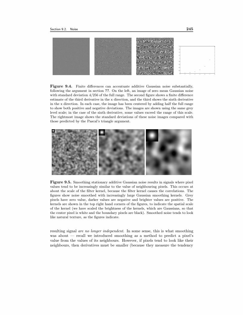
Figure 9.5. Smoothing stationary additive Gaussian noise results in signals where pixelvalues tend to be increasingly similar to the value of neighbouring pixels. This occurs atabout the scale of the filter kernel, because the filter kernel causes the correlations. Thefigures show noise smoothed with increasingly large Gaussian smoothing kernels. Greypixels have zero value, darker values are negative and brighter values are positive. Thekernels are shown in the top right hand corners of the figures, to indicate the spatial scaleof the kernel (we have scaled the brightness of the kernels, which are Gaussians, so thatthe center pixel is white and the boundary pixels are black). Smoothed noise tends to looklike natural texture, as the figures indicate.

resulting signal are no longer independent. In some sense, this is what smoothingwas about — recall we introduced smoothing as a method to predict a pixel’svalue from the values of its neighbours. However, if pixels tend to look like theirneighbours, then derivatives must be smaller (because they measure the tendency


of pixels to look different from their neighbours).Smoothed noise has applications. As figure 9.5 indicates, smoothed noise tends

to look like some kinds of natural texture, and smoothed noise is quite widely usedas a source of textures in computer graphics applications []).

Difficulties with the Additive Stationary Gaussian Noise Model

Taken literally, the additive stationary Gaussian noise model is poor model of imagenoise. Firstly, the model allows positive (and, more alarmingly, negative!) pixelvalues of arbitrary magnitude. With appropriate choices of standard deviation fortypical current cameras operating indoors or in daylight, this doesn’t present muchof a problem, because these pixel values are extremely unlikely to occur in practice.In rendering noise images, the problematic pixels that do occur are fixed at zero orfull output respectively.

Secondly, noise values are completely independent, so this model does not cap-ture the possibility of groups of pixels that have correlated responses, perhaps be-cause of the design of the camera electronics or because of hot spots in the cameraintegrated circuit. This problem is harder to deal with, because noise models thatdo model this effect tend to be difficult to deal with analytically. Finally, this modeldoes not describe “dead pixels” (pixels that consistently report no incoming light,or are consistently saturated) terribly well. If the standard deviation is quite largeand we threshold pixel values, then dead pixels will occur, but the standard devi-ation may be too large to model the rest of the image well. A crucial advantageof additive Gaussian noise is that it is easy to estimate the response of filters tothis noise model. In turn, this gives us some idea of how effective the filter is atresponding to signal and ignoring noise.

9.3 Edges and Gradient-based Edge Detectors

Sharp changes in image brightness are interesting for many reasons. Firstly, objectboundaries often generate sharp changes in brightness — a light object may lieon a dark background, or a light object may lie on a dark background. Secondly,reflectance changes often generate sharp changes in brightness which can be quitedistinctive — zebras have stripes and leopards have spots. Cast shadows can alsogenerate sharp changes in brightness. Finally, sharp changes in surface orientationare often associated with sharp changes in image brightness.

Points in the image where brightness changes particularly sharply are oftencalled edges or edge points. We should like edge points to be associated withthe boundaries of objects and other kinds of meaningful changes. It is hard todefine precisely the changes we would like to mark — is the region of a pastoralscene where the leaves give way to the sky the boundary of an object? Typically,it is hard to tell a semantically meaningful edge from a nuisance edge, and to doso requires a great deal of high-level information. Nonetheless, experience buildingvision systems suggests that very often, interesting things are happening in an image

Section 9.3. Edges and Gradient-based Edge Detectors 247

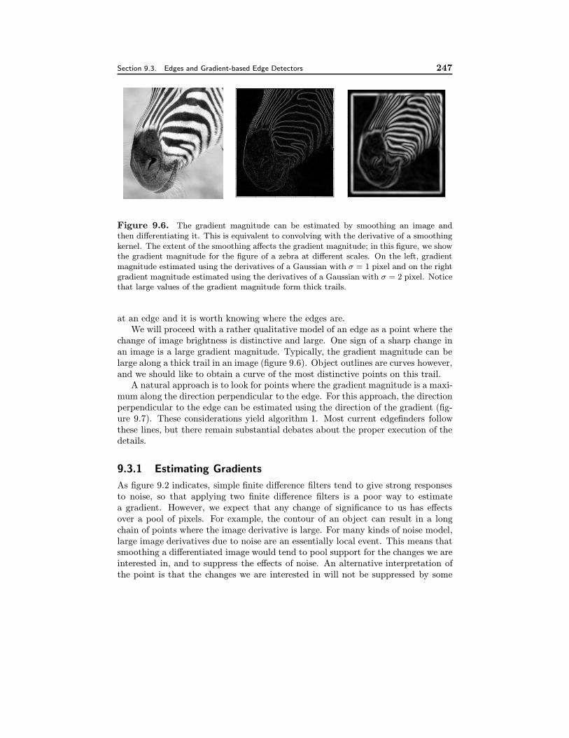
Figure 9.6. The gradient magnitude can be estimated by smoothing an image andthen differentiating it. This is equivalent to convolving with the derivative of a smoothingkernel. The extent of the smoothing affects the gradient magnitude; in this figure, we showthe gradient magnitude for the figure of a zebra at different scales. On the left, gradientmagnitude estimated using the derivatives of a Gaussian with σ = 1 pixel and on the rightgradient magnitude estimated using the derivatives of a Gaussian with σ = 2 pixel. Noticethat large values of the gradient magnitude form thick trails.

at an edge and it is worth knowing where the edges are.We will proceed with a rather qualitative model of an edge as a point where the

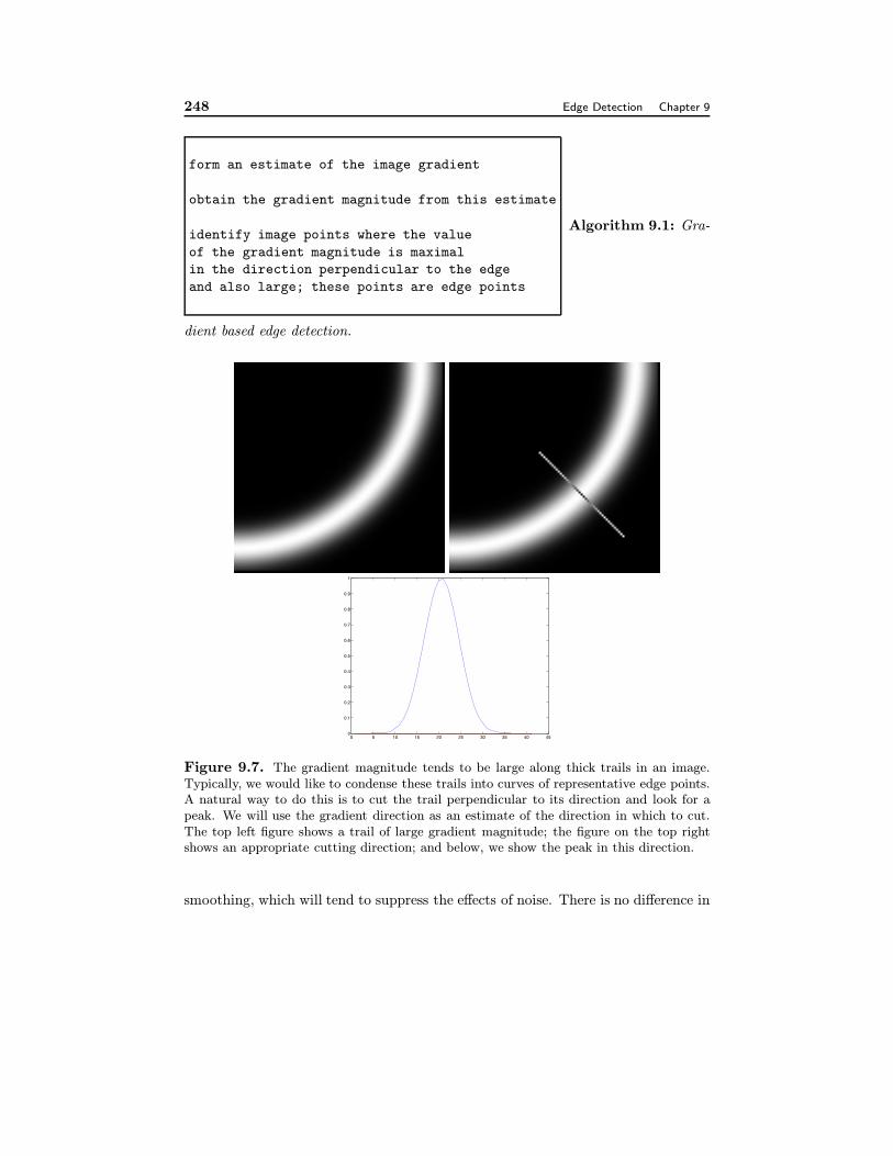
change of image brightness is distinctive and large. One sign of a sharp change inan image is a large gradient magnitude. Typically, the gradient magnitude can belarge along a thick trail in an image (figure 9.6). Object outlines are curves however,and we should like to obtain a curve of the most distinctive points on this trail.

A natural approach is to look for points where the gradient magnitude is a maxi-mum along the direction perpendicular to the edge. For this approach, the directionperpendicular to the edge can be estimated using the direction of the gradient (fig-ure 9.7). These considerations yield algorithm 1. Most current edgefinders followthese lines, but there remain substantial debates about the proper execution of thedetails.

9.3.1 Estimating Gradients

As figure 9.2 indicates, simple finite difference filters tend to give strong responsesto noise, so that applying two finite difference filters is a poor way to estimatea gradient. However, we expect that any change of significance to us has effectsover a pool of pixels. For example, the contour of an object can result in a longchain of points where the image derivative is large. For many kinds of noise model,large image derivatives due to noise are an essentially local event. This means thatsmoothing a differentiated image would tend to pool support for the changes we areinterested in, and to suppress the effects of noise. An alternative interpretation ofthe point is that the changes we are interested in will not be suppressed by some


form an estimate of the image gradient

obtain the gradient magnitude from this estimate

identify image points where the value

of the gradient magnitude is maximal

in the direction perpendicular to the edge

and also large; these points are edge points

Algorithm 9.1: Gra-

dient based edge detection.

0 5 10 15 20 25 30 35 40 450

0.1

0.2

0.3

0.4

0.5

0.6

0.7

0.8

0.9

1

Figure 9.7. The gradient magnitude tends to be large along thick trails in an image.Typically, we would like to condense these trails into curves of representative edge points.A natural way to do this is to cut the trail perpendicular to its direction and look for apeak. We will use the gradient direction as an estimate of the direction in which to cut.The top left figure shows a trail of large gradient magnitude; the figure on the top rightshows an appropriate cutting direction; and below, we show the peak in this direction.

smoothing, which will tend to suppress the effects of noise. There is no difference in


principle between differentiating a smoothed image, or smoothing a differentiatedimage.

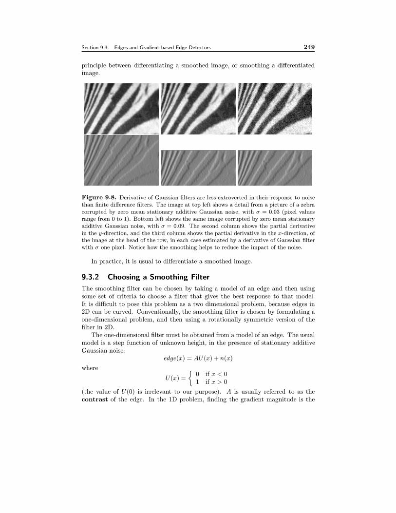
Figure 9.8. Derivative of Gaussian filters are less extroverted in their response to noisethan finite difference filters. The image at top left shows a detail from a picture of a zebracorrupted by zero mean stationary additive Gaussian noise, with σ = 0.03 (pixel valuesrange from 0 to 1). Bottom left shows the same image corrupted by zero mean stationaryadditive Gaussian noise, with σ = 0.09. The second column shows the partial derivativein the y-direction, and the third column shows the partial derivative in the x-direction, ofthe image at the head of the row, in each case estimated by a derivative of Gaussian filterwith σ one pixel. Notice how the smoothing helps to reduce the impact of the noise.

In practice, it is usual to differentiate a smoothed image.

9.3.2 Choosing a Smoothing Filter

The smoothing filter can be chosen by taking a model of an edge and then usingsome set of criteria to choose a filter that gives the best response to that model.It is difficult to pose this problem as a two dimensional problem, because edges in2D can be curved. Conventionally, the smoothing filter is chosen by formulating aone-dimensional problem, and then using a rotationally symmetric version of thefilter in 2D.

The one-dimensional filter must be obtained from a model of an edge. The usualmodel is a step function of unknown height, in the presence of stationary additiveGaussian noise:

edge(x) = AU(x) + n(x)

where

U(x) =

{0 if x < 01 if x > 0

(the value of U(0) is irrelevant to our purpose). A is usually referred to as thecontrast of the edge. In the 1D problem, finding the gradient magnitude is the


same as finding the square of the derivative response. For this reason, we usuallyseek a derivative estimation filter rather than a smoothing filter (which can then bereconstructed by integrating the derivative estimation filter).

Canny established the practice of choosing a derivative estimation filter by usingthe continuous model to optimize a combination of three criteria:

• Signal to noise ratio — the filter should respond more strongly to the edgeat x = 0 than to noise.

• Localisation — the filter response should reach a maximum very close tox = 0.

• Low false positives — there should be only one maximum of the responsein a reasonable neighbourhood of x = 0.

Once a continuous filter has been found, it is discretised. The criteria can becombined in a variety of ways, yielding a variety of somewhat different filters. Itis a remarkable fact that the optimal smoothing filters that are derived by mostcombinations of these criteria tend to look a great deal like Gaussians — this isintuitively reasonable, as the smoothing filter must place strong weight on centerpixels and less weight on distant pixels, rather like a Gaussian. In practice, optimalsmoothing filters are usually replaced by a Gaussian, with no particularly importantdegradation in performance.

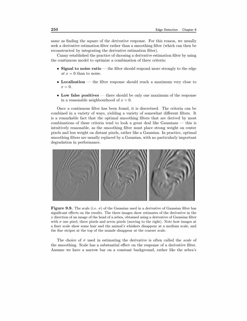
Figure 9.9. The scale (i.e. σ) of the Gaussian used in a derivative of Gaussian filter hassignificant effects on the results. The three images show estimates of the derivative in thex direction of an image of the head of a zebra, obtained using a derivative of Gaussian filterwith σ one pixel, three pixels and seven pixels (moving to the right). Note how images ata finer scale show some hair and the animal’s whiskers disappear at a medium scale, andthe fine stripes at the top of the muzzle disappear at the coarser scale.

The choice of σ used in estimating the derivative is often called the scale ofthe smoothing. Scale has a substantial effect on the response of a derivative filter.Assume we have a narrow bar on a constant background, rather like the zebra’s


whisker. Smoothing on a scale smaller than the width of the bar will mean that thefilter responds on each side of the bar, and we will be able to resolve the rising andfalling edges of the bar. If the filter width is much greater, the bar will be smoothedinto the background, and the bar will generate little or no response (as figure 9.9).

9.3.3 Why Smooth with a Gaussian?

While a Gaussian is not the only possible blurring kernel, it is convenient becauseit has a number of important properties. Firstly, if we convolve a Gaussian with aGaussian, and the result is another Gaussian:

Gσ1 ∗ ∗Gσ2 = G√σ2

1+σ22

This means that it is possible to obtain very heavily smoothed images by resmooth-ing smoothed images. This is a significant property, firstly because discrete convo-lution can be an expensive operation (particularly if the kernel of the filter is large),and secondly because it is common to want to see versions of an image smoothedby different amounts.

Efficiency

Consider convolving an image with a Gaussian kernel with σ one pixel. Althoughthe Gaussian kernel is non zero over an infinite domain, for most of that domainit is extremely small because of the exponential form. For σ one pixel, pointsoutside a 5x5 integer grid centered at the origin have values less than e−4 = 0.0184and points outside a 7x7 integer grid centered at the origin have values less thane−9 = 0.0001234. This means that we can ignore their contributions, and representthe discrete Gaussian as a small array (5x5 or 7x7, according to taste and thenumber of bits you allocate to representing the kernel).

However, if σ is 10 pixels, we may need a 50x50 array or worse. A back ofthe envelope count of operations should convince you that convolving a reasonablysized image with a 50x50 array is an unattractice prospect. The alternative —convolving repeatedly with a much smaller kernel — is much more efficient, becausewe don’t need to keep every pixel in the interim. This is because a smoothed imageis, to some extent, redundant (most pixels contain a significant component of theirneighbours’ values). As a result, some pixels can be discarded. We then have astrategy which is quite efficient: smooth, subsample, smooth, subsample, etc. Theresult is an image that has the same information as a heavily smoothed image, butis very much smaller and is easier to obtain. We explore the details of this approachin section 9.4.1.

The Central Limit Theorem

Gaussians have another significant property which we shall not prove but illustratein figure 9.10. For an important family of functions, convolving any member of thatfamily of functions with itself repeatedly will eventually yield a Gaussian. With


0 20 40 60 80 100 1200

0.01

0.02

0.03

0.04

0.05

0.06

0.07

0.08

0.09

0.1

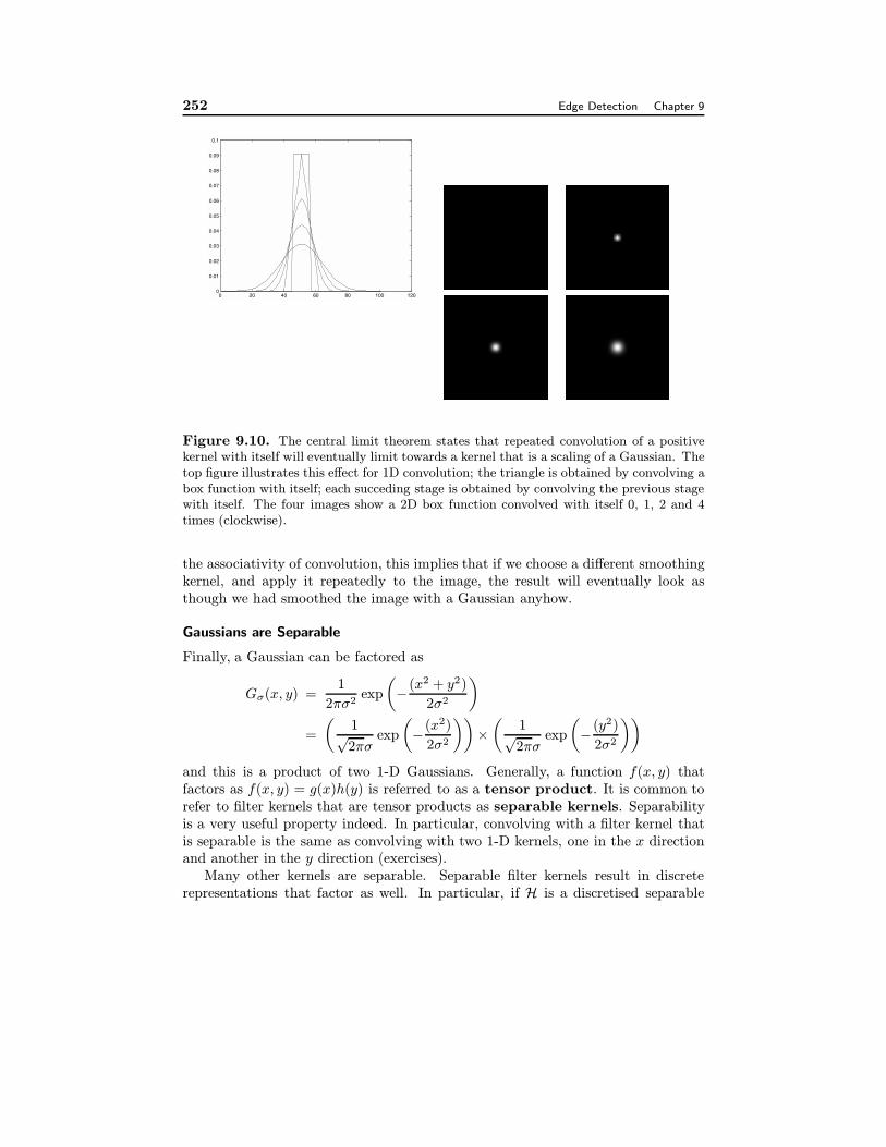
Figure 9.10. The central limit theorem states that repeated convolution of a positivekernel with itself will eventually limit towards a kernel that is a scaling of a Gaussian. Thetop figure illustrates this effect for 1D convolution; the triangle is obtained by convolving abox function with itself; each succeding stage is obtained by convolving the previous stagewith itself. The four images show a 2D box function convolved with itself 0, 1, 2 and 4times (clockwise).

the associativity of convolution, this implies that if we choose a different smoothingkernel, and apply it repeatedly to the image, the result will eventually look asthough we had smoothed the image with a Gaussian anyhow.

Gaussians are Separable

Finally, a Gaussian can be factored as

Gσ(x, y) =1

2πσ2exp

(−(x2 + y2)

2σ2

)

=

(1

√2πσ

exp

(−(x2)

2σ2

))×

(1

√2πσ

exp

(−(y2)

2σ2

))

and this is a product of two 1-D Gaussians. Generally, a function f(x, y) thatfactors as f(x, y) = g(x)h(y) is referred to as a tensor product. It is common torefer to filter kernels that are tensor products as separable kernels. Separabilityis a very useful property indeed. In particular, convolving with a filter kernel thatis separable is the same as convolving with two 1-D kernels, one in the x directionand another in the y direction (exercises).

Many other kernels are separable. Separable filter kernels result in discreterepresentations that factor as well. In particular, if H is a discretised separable


filter kernel, then there are some vectors f and g such that

Hij = figj

It is possible to identify this property using techniques from numerical linear algebra;commercial convolution packages often test the kernel to see if it is separable beforeapplying it to the image. The cost of this test is easily paid off by the savings if thekernel does turn out to be separable.

9.3.4 Derivative of Gaussian Filters

Smoothing an image and then differentiating it is the same as convolving it with thederivative of a smoothing kernel. This fact is most easily seen by thinking aboutcontinuous convolution.

Firstly, differentiation is linear and shift invariant. This means that there issome kernel — we dodge the question of what it looks like — that differentiates.That is, given a function I(x, y)

∂I

∂x= K ∂

∂x∗ ∗I

Now we want the derivative of a smoothed function. We write the convolutionkernel for the smoothing as S. Recalling that convolution is associative, we have

(K ∂∂x∗ ∗(S ∗ ∗I)) = (K ∂

∂x∗ ∗S) ∗ ∗I = (

∂S

∂x) ∗ ∗I

This fact appears in its most commonly used form when the smoothing function isa Gaussian; we can then write

∂ (Gσ ∗ ∗I)

∂x= (∂Gσ

∂x) ∗ ∗I

i.e. we need only convolve with the derivative of the Gaussian, rather than convolveand then differentiate. A similar remark applies to the Laplacian. Recall that theLaplacian of a function in 2D is defined as:

(∇2f)(x, y) =∂2f

∂x2+∂2f

∂y2

Again, because convolution is associative, we have that

(K∇2 ∗ ∗(Gσ ∗ ∗I)) = (K∇2 ∗ ∗Gσ) ∗ ∗I = (∇2Gσ) ∗ ∗I

This practice results in much smaller noise responses from the derivative esti-mates (figure 9.8).


Gradient

p

q

r

r

sGradient

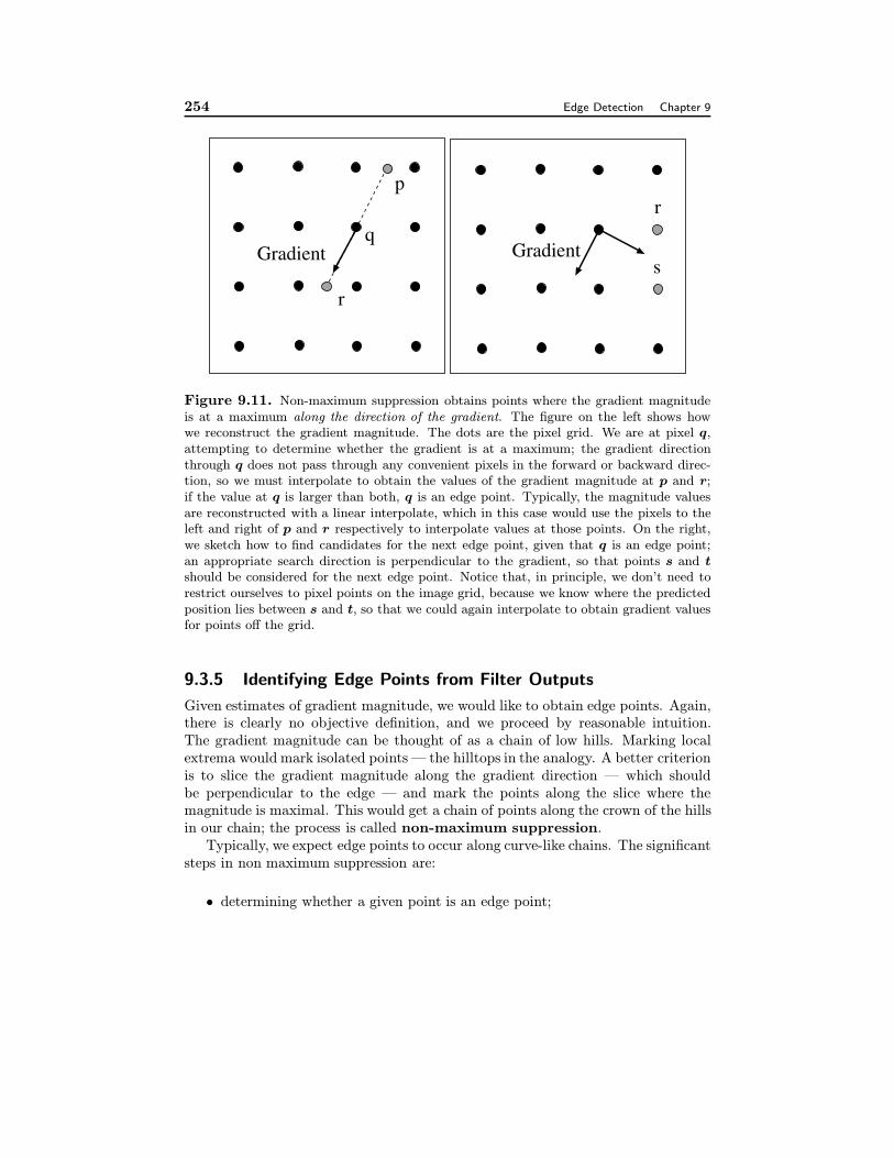
Figure 9.11. Non-maximum suppression obtains points where the gradient magnitudeis at a maximum along the direction of the gradient. The figure on the left shows howwe reconstruct the gradient magnitude. The dots are the pixel grid. We are at pixel q,attempting to determine whether the gradient is at a maximum; the gradient directionthrough q does not pass through any convenient pixels in the forward or backward direc-tion, so we must interpolate to obtain the values of the gradient magnitude at p and r;if the value at q is larger than both, q is an edge point. Typically, the magnitude valuesare reconstructed with a linear interpolate, which in this case would use the pixels to theleft and right of p and r respectively to interpolate values at those points. On the right,we sketch how to find candidates for the next edge point, given that q is an edge point;an appropriate search direction is perpendicular to the gradient, so that points s and tshould be considered for the next edge point. Notice that, in principle, we don’t need torestrict ourselves to pixel points on the image grid, because we know where the predictedposition lies between s and t, so that we could again interpolate to obtain gradient valuesfor points off the grid.

9.3.5 Identifying Edge Points from Filter Outputs

Given estimates of gradient magnitude, we would like to obtain edge points. Again,there is clearly no objective definition, and we proceed by reasonable intuition.The gradient magnitude can be thought of as a chain of low hills. Marking localextrema would mark isolated points — the hilltops in the analogy. A better criterionis to slice the gradient magnitude along the gradient direction — which shouldbe perpendicular to the edge — and mark the points along the slice where themagnitude is maximal. This would get a chain of points along the crown of the hillsin our chain; the process is called non-maximum suppression.

Typically, we expect edge points to occur along curve-like chains. The significantsteps in non maximum suppression are:

• determining whether a given point is an edge point;


• and, if it is, finding the next edge point.

Once these steps are understood, it is easy to enumerate all edge chains. We findthe first edge point, mark it, expand all chains through that point exhaustively,marking all points along those chains, and continue to do this for all unmarkededge points.

While there are points with high gradient

that have not been visited

Find a start point that is a local maximum in the

direction perpendicular to the gradient

erasing points that have been checked

while possible, expand a chain through

the current point by:

1) predicting a set of next points, using

the direction perpendicular to the gradient

2) finding which (if any) is a local maximum

in the gradient direction

3) testing if the gradient magnitude at the

maximum is sufficiently large

4) leaving a record that the point and

neighbours have been visited

record the next point, which becomes the current point

end

end

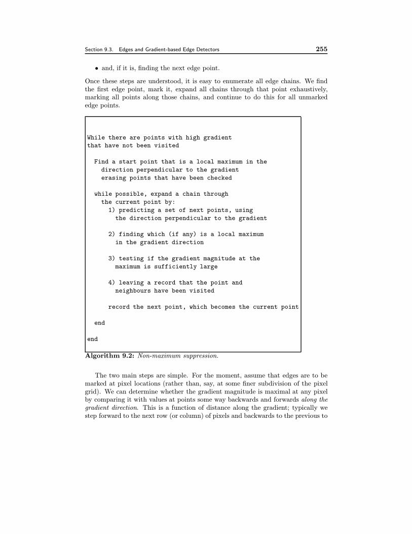
Algorithm 9.2: Non-maximum suppression.

The two main steps are simple. For the moment, assume that edges are to bemarked at pixel locations (rather than, say, at some finer subdivision of the pixelgrid). We can determine whether the gradient magnitude is maximal at any pixelby comparing it with values at points some way backwards and forwards along thegradient direction. This is a function of distance along the gradient; typically westep forward to the next row (or column) of pixels and backwards to the previous to


determine whether the magnitude at our pixel is larger (figure 9.11). The gradientdirection does not usually pass through the next pixel, so we must interpolate todetermine the value of the gradient magnitude at the points we are interested in; alinear interpolate is usual.

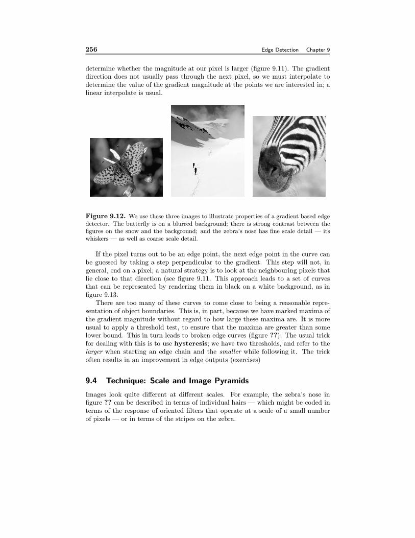
Figure 9.12. We use these three images to illustrate properties of a gradient based edgedetector. The butterfly is on a blurred background; there is strong contrast between thefigures on the snow and the background; and the zebra’s nose has fine scale detail — itswhiskers — as well as coarse scale detail.

If the pixel turns out to be an edge point, the next edge point in the curve canbe guessed by taking a step perpendicular to the gradient. This step will not, ingeneral, end on a pixel; a natural strategy is to look at the neighbouring pixels thatlie close to that direction (see figure 9.11. This approach leads to a set of curvesthat can be represented by rendering them in black on a white background, as infigure 9.13.

There are too many of these curves to come close to being a reasonable repre-sentation of object boundaries. This is, in part, because we have marked maxima ofthe gradient magnitude without regard to how large these maxima are. It is moreusual to apply a threshold test, to ensure that the maxima are greater than somelower bound. This in turn leads to broken edge curves (figure ??). The usual trickfor dealing with this is to use hysteresis; we have two thresholds, and refer to thelarger when starting an edge chain and the smaller while following it. The trickoften results in an improvement in edge outputs (exercises)

9.4 Technique: Scale and Image Pyramids

Images look quite different at different scales. For example, the zebra’s nose infigure ?? can be described in terms of individual hairs — which might be coded interms of the response of oriented filters that operate at a scale of a small numberof pixels — or in terms of the stripes on the zebra.

Section 9.4. Technique: Scale and Image Pyramids 257

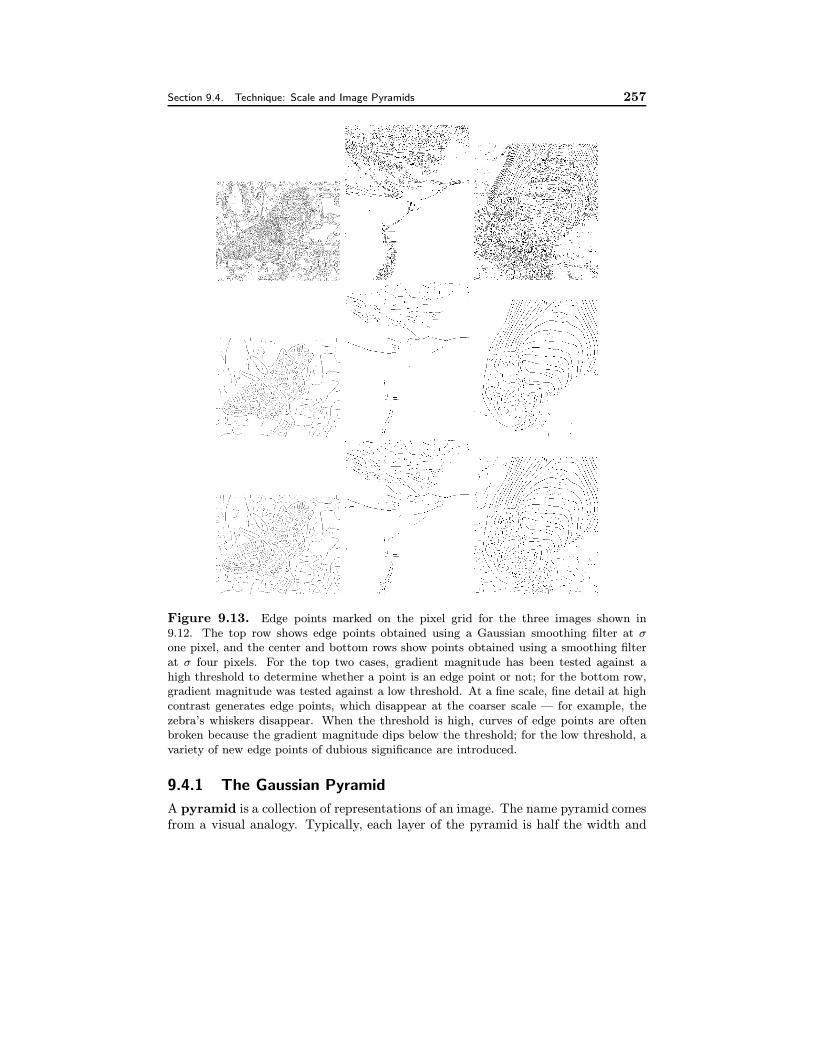
Figure 9.13. Edge points marked on the pixel grid for the three images shown in9.12. The top row shows edge points obtained using a Gaussian smoothing filter at σone pixel, and the center and bottom rows show points obtained using a smoothing filterat σ four pixels. For the top two cases, gradient magnitude has been tested against ahigh threshold to determine whether a point is an edge point or not; for the bottom row,gradient magnitude was tested against a low threshold. At a fine scale, fine detail at highcontrast generates edge points, which disappear at the coarser scale — for example, thezebra’s whiskers disappear. When the threshold is high, curves of edge points are oftenbroken because the gradient magnitude dips below the threshold; for the low threshold, avariety of new edge points of dubious significance are introduced.

9.4.1 The Gaussian Pyramid

A pyramid is a collection of representations of an image. The name pyramid comesfrom a visual analogy. Typically, each layer of the pyramid is half the width and


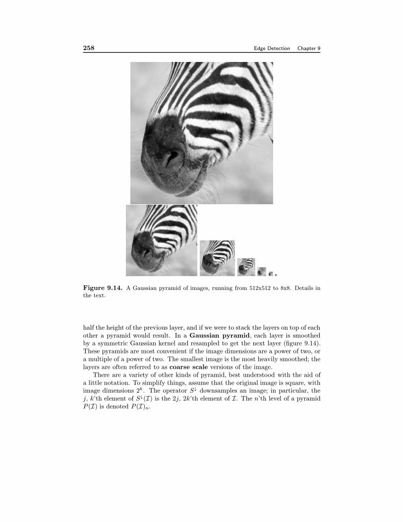
Figure 9.14. A Gaussian pyramid of images, running from 512x512 to 8x8. Details inthe text.

half the height of the previous layer, and if we were to stack the layers on top of eachother a pyramid would result. In a Gaussian pyramid, each layer is smoothedby a symmetric Gaussian kernel and resampled to get the next layer (figure 9.14).These pyramids are most convenient if the image dimensions are a power of two, ora multiple of a power of two. The smallest image is the most heavily smoothed; thelayers are often referred to as coarse scale versions of the image.

There are a variety of other kinds of pyramid, best understood with the aid ofa little notation. To simplify things, assume that the original image is square, withimage dimensions 2k. The operator S↓ downsamples an image; in particular, thej, k’th element of S↓(I) is the 2j, 2k’th element of I. The n’th level of a pyramidP (I) is denoted P (I)n.


We can now write simple expressions for the layers of a Gaussian pyramid:

PGaussian(I)n+1 = S↓(Gσ ∗ ∗PGaussian(I)n) (9.4.1)

= (S↓Gσ)PGaussian(I)n) (9.4.2)

(where we have written Gσ for the linear operator that takes an image to theconvolution of that image with a Gaussian). The finest scale layer is the originalimage

PGaussian(I)1 = I

A simple, immediate use for a Gaussian pyramid is to obtain zero-crossings of aLaplacian of Gaussian (or a DOG) at various levels of smoothing.

Set the finest scale layer to the image

For each layer, going from next to finest to coarsest

Obtain this layer by smoothing the next finest

layer with a Gaussian, and then subsampling it

end

Algorithm

9.3: Forming a Gaussian pyramid

9.4.2 Applications of Scaled Representations

Gaussian pyramids are useful, because they make it possible to extract representa-tions of different types of structure in an image. For example, in the case of thezebra, we would not want to apply very large filters to find the stripes. This isbecause these filters are inclined to spurious precision — we don’t wish to have torepresent the disposition of each hair on the stripe — inconvenient to build, andslow to apply.

A more practical approach than applying very large filters is to apply smallerfilters to a less detailed version of the image. We expect effects to appear at avariety of scales, and so represent the image in terms of several smoothed andsampled versions. Continuing with the zebra analogy, this means we can representthe hair on the animal’s nose, the stripes of its body, dark legs, and entire zebras,each as bars of different sizes.


Scale and Spatial Search

Another application is spatial search, a common theme in computer vision. Typi-cally, we have a point in one image and are trying to find a point in a second imagethat corresponds to it. This problem occurs in stereopsis — where the point hasmoved because the two images are obtained from different viewing positions — andin motion analysis — where the image point has moved either because the cameramoved, or because it is on a moving object.

Searching for a match in the original pairs of images is inefficient, because wemay have to wade through a great deal of detail. A better approach, which is nowpretty much universal, is to look for a match in a heavily smoothed and resampledimage, and then refine that match by looking at increasingly detailed versions ofthe image. For example, we might reduce 1024x1024 images down to 4x4 versions,match those and then look at 8x8 versions (because we know a rough match, it iseasy to refine it); we then look at 16x16 versions, etc. all the way up to 1024x1024.This gives an extremely efficient search, because a step of a single pixel in the 4x4version is equivalent to a step of 256 pixels in the 1024x1024 version. We will explorethis strategy of coarse-to-fine matching in greater detail in chapters ??.

Edge Tracking

Most edges found at coarse levels of smoothing tend are associated with large, highcontrast image events, because for an edge to be marked at a coarse scale a largepool of pixels need to agree that there is a high contrast edge. Typically, theseedges understate the extent of a feature — the contrast might decay along the edge,for example — and their localisation can be quite poor — a single pixel error in acoarse-scale image represents a multiple pixel error in a fine-scale image.

At fine scales, there are many edges, some of which are associated with smaller,low contrast events. One strategy for improving a set of edges obtained at a finescale is to track edges across scales to a coarser scale, and accept only the fine scaleedges that have identifiable parents at a coarser scale. This strategy in principlecan suppress edges resulting from textured regions (often referred to as “noise”)and edges resulting from real noise.

9.4.3 Scale Space

Coarse scale components give the overall structure of a signal, and fine scale com-ponents give detailed information, as figure ?? suggests. This approach allows usto think about representing such objects as trees, which appear to exist at severaldistinct scales; we would want to be able to represent a tree both as a puff of foliageon top of a stalk (coarse scale) and as a collection of individual leaves and twigs(fine scale).

Gaussian pyramids are not an ideal tool for this representation, because theysample the range of smoothed images quite coarsely. Instead of a discrete pyramidof images, we might consider a one parameter family of images (or, equivalently, a


Figure 9.15. Edge tracking

function of three dimensions)

Φ(x, y, u) = Gσ(u) ∗ I(x, y)

where the extent of the smoothing is now a continuous parameter. For a 1D signal,we can draw the behaviour of features as the scaling parameter changes, and thisdrawing gives us a simple and sometimes quite informative description of the signal(figure ??). If we define a “feature” to be a zero-crossing of the Laplacian, thenit is possible to show that in this family of images, features are not created bysmoothing. This means that all coarse-scale zero-crossings will have finer-scaleevents corresponding to them, so that there are quite simple rules for what thesedrawings look like (figure ??). These drawings and the underlying representationsare often referred to as scale space.

If we think of the signal as being composed of a set of parametric patches joinedat these feature points, we obtain a different decomposition of the signal at eachscale. Instead of representing the signal with a continuous family of decompositionswhere the feature points move, we could fix the location of these feature points andthen use the simple rules for constructing scale-space drawings to obtain a strip-likedecomposition (as in figure ??). This is not a decomposition with a canonical form— we get to choose what the features are and the nature of the parametric patches— but it is often rather useful in practice, mainly because the decomposition of thesignal appears to reflect the structure apparent to humans.

2D scale space

It is possible to extend these decompositions from 1D to 2D. Again, the choiceof features is somewhat open, but a reasonable choice is the points of maximumor minimum brightness. Smoothing an image with a symmetric Gaussian cannotcreate local maxima or minima in brightness, but it can (and does) destroy them.Assume we have a scale value σdie where a maximum (or minimum — we will justtalk about the one case, for simplicity) is destroyed. If we now reduce the scale, astandard pattern will appear — there will be a corresponding maximum surrounded


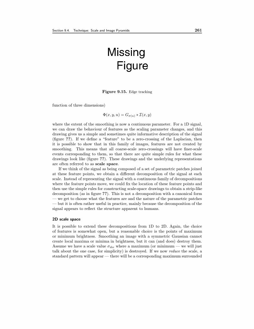
Figure 9.16. On the left, a 1D signal smoothed using Gaussian filters of increasing σ(scale increases vertically; the signal is a function of the horizontal coordinate). As thesignal is smoothed, extrema merge and vanish. The smoothest versions of the signal canbe seen as an indication of the “overall trend” of the signal, and the finer versions haveincreasing amounts of detail imposed. The representation on the left marks the position ofzero crossings of the second derivative of the smoothed signal, as the smoothing increases(again, scale increases vertically). Notice that zero crossings can meet and obliterate oneanother as the signal is smoothed but no new zero-crossing is created. This means that thefigure shows the characteristic structure of either vertical curves or inverted “u” curves.An inverted pitchfork shape is also possible — where three extrema meet and become one— but this requires special properties of the signal and usually becomes an inverted u nextto a vertical curve. Notice also that the position of zero crossings tends to shift as thesignal is smoothed. Figure from “Scale-space filtering,” A.P. Witkin, Proc. 8’th IJCAI,1983, page 1020, in the fervent hope, etc.

by a curve of equal brightness that has a self intersection. Thus, corresponding toeach maximum (or minimum) at any scale, we have a blob, which is the regionof the image marked out by this curve of equal brightness. Typically, maximaare represented by light blobs and minima by dark blobs. All of this gives us arepresentation of an image in terms of blobs growing (or dying) as the scale isdecreased (or increased).

9.4.4 Anisotropic Scaling

One important difficulty with scale space models is that the symmetric Gaussiansmoothing process tends to blur out edges rather two aggressively for comfort. Forexample, if we have two trees near one another on a skyline, the large scale blobscorresponding to each tree may start merging before all the small scale blobs havefinished. This suggests that we should smooth differently at edge points than atother points. For example, we might make an estimate of the magnitude and orien-tation of the gradient: for large gradients, we would then use an oriented smoothing


- + + - + - +

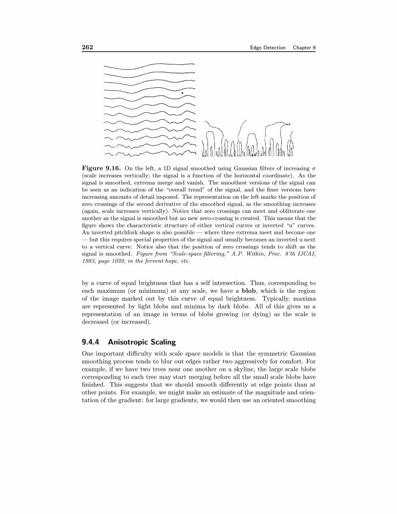
Figure 9.17. Smoothing an image with a symmetric Gaussian cannot create local max-ima or local minima of brightness. However, local extrema can be extinguished. Whathappens is that a local maximum shrinks down to the value of the surrounding pixels. Thisis most easily conveyed by drawing a contour plot — the figure shows a contour plot witha local maximum which dies as the image is smoothed (the curve is a contour of constantbrightness; the regions marked + have brightness greater than that of the contour, so theblob must have a maximum in it; the regions marked - have brightness less than that ofthe contour). Recording the details of these disappearances — where the maximum thatdisappears is, the contour defining the blob around the maximum, and the scale at whichit disappears — yields a scale-space representation of the image.

operator that smoothed aggressively perpendicular to the gradient and very littlealong the gradient; for small gradients, we might use a symmetric smoothing oper-ator. This idea used to be known as edge preserving smoothing.

In the modern, more formal version (details in in []), we notice the scale spacerepresentation family is a solution to the diffusion equation

∂Φ

∂σ=∂2Φ

∂x2+∂2Φ

∂y2

= ∇2Φ

Φ(x, y, 0) = I(x, y)

If this equation is modified to have the form

∂Φ

∂σ= ∇ · (c(x, y, σ)∇Φ)

= c(x, y, σ)∇2Φ+ (∇c(x, y, σ)) · (∇Φ)

Φ(x, y, 0) = I(x, y)

then if c(x, y, σ) = 1, we have the diffusion equation we started with, and ifc(x, y, σ) = 0 there is no smoothing. We will assume that c does not dependon σ. If we knew where the edges were in the image, we could construct a maskthat consisted of regions where c(x, y) = 1, isolated by patches along the edgeswhere c(x, y) = 0; in this case, a solution would smooth inside each separate region,but not over the edge. While we do not know where the edges are — the exercisewould be empty if we did — we can obtain reasonable choices of c(x, y) from the


magnitude of the image gradient. If the gradient is large, then c should be small,and vice-versa.

9.5 Human Vision: More of the Visual Pathway

9.5.1 The Lateral Geniculate Nucleus

The LGN is a layered structure, consisting of many sheets of neurons. The layers aredivided into two classes — those consisting of cells with large cell bodies (magno-cellular layers), and those consisting of cells with small cell bodies (parvocellularlayers). The behaviour of these cells differs as well.

Each layer in the LGN receives input from a single eye, and is laid out likethe retina of the eye providing input (an effect known as retinotopic mapping).Retinotopic mapping means that nearby regions on the retina end up near oneanother in the layer, and so we can think of each layer as representing some formof feature map. Neurons in the lateral geniculate nucleus display similar receptivefield behaviour to retinal neurons. The role of the LGN is unclear; it is known thatthe LGN receives input from the cortex and from other regions of the brain, whichmay modify the visual signal travelling from the retina to the cortex.

9.5.2 The Visual Cortex

Most visual signals arrive at an area of the cortex called area V1 (or the primaryvisual cortex, or the striate cortex). This area is highly structured and has beenintensively studied. Most physiological information about the cortex comes fromstudies of cats or monkeys (which are known to react differently from one anotherand from humans if the cortex is damaged). The cortex is also retinotopicallymapped. It has a highly structured layered architecture, with regions organised bythe eye of origin of the signal (often called ocular dominance columns). Withinthese columns, cells are arranged so that their receptive fields move smoothly fromthe center to the periphery of the visual field. Neurons in the primary visual cortexhave been extensively studied. Two classes are usually recognised — simple cellsand complex cells.

Simple cells have orientation selective receptive fields, meaning that a partic-ular cell will respond more strongly to an oriented structure. To a good approxima-tion, the response of a simple cell is linear, so that the behaviour of these cells canbe modelled with spatial filters. The structure of typical receptive fields means thatthese cells can be thought of as edge and bar detectors [?], or as first and secondderivative operators. Some simple cells have more lobes to their receptive field, andcan be thought of as detecting higher derivatives. The preferred orientation of acell varies fairly smoothly in a principled way that depends on the cell’s position.

Complex cells typically are highly non-linear, and respond to moving edges orbars. Typically, the cells display direction selectivity, in that the response of a cellto a moving bar depends strongly on both the orientation of the bar and the direction

Section 9.5. Human Vision: More of the Visual Pathway 265

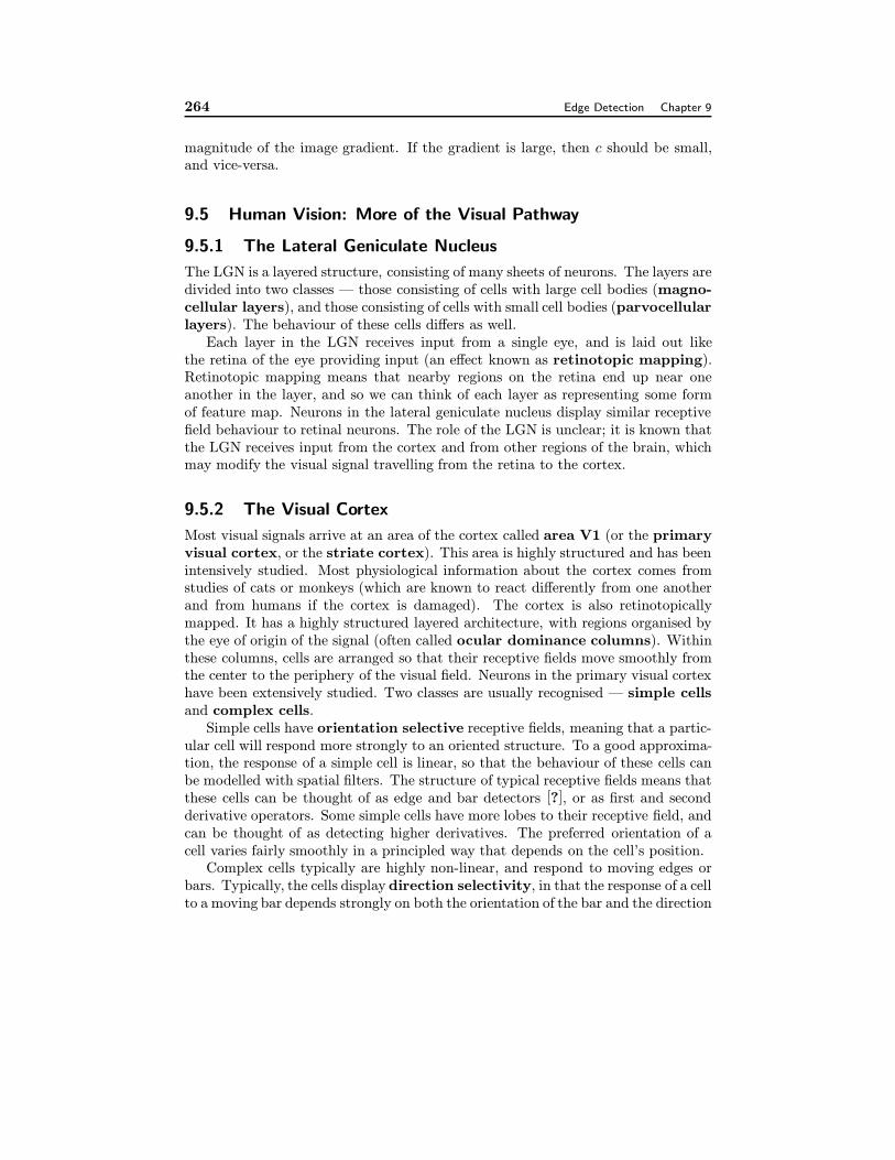
Figure 9.18. Receptive fields of some cortical simple cells, which can be modelled aslinear. ‘+’ signs mean that light in the area excites the cell; ‘-’ signs means that it inhibitsthe cell. Notice that these cells are orientation selective; the cell on the left respondsmost strongly to a bright bar on a dark background, the cell on the center will respondmost strongly to a dark bar off center on a light background, and the cell on the rightwill respond strongly to an oriented edge. Figure from John Dowling’s book “Neurons andNetworks - an introduction to neuroscience”, page 336, in the fervent hope that permissionwill be granted Notice the similarity to the derivative of Gaussian filters plotted on below.

of the motion (figure 9.19). Some complex cells, often called hypercomplex cellsrespond preferentially to bars of a particular length.

One strong distinction between simple and complex cells appears when one con-siders the time-course of a response to a contrast reversing pattern— a spatialsinusoid whose amplitude is a sinusoidal function of time. Exposed to such a stim-ulus, a simple cell responds strongly for the positive contrast and not at all forthe negative contrast — it is trying to be linear, but because the resting responseof the cell is low, there is a limit to the extent to which the cell’s output can beinhibited. In contrast, complex cells respond to both phases (figure 9.20). Thus,one can think of a simple cell as performing half-wave rectification — it respondsto the positive half of the amplitude signal — and a complex cell as performing fullwave rectification — it gives a response to both the positive and negative half ofthe amplitude signal.


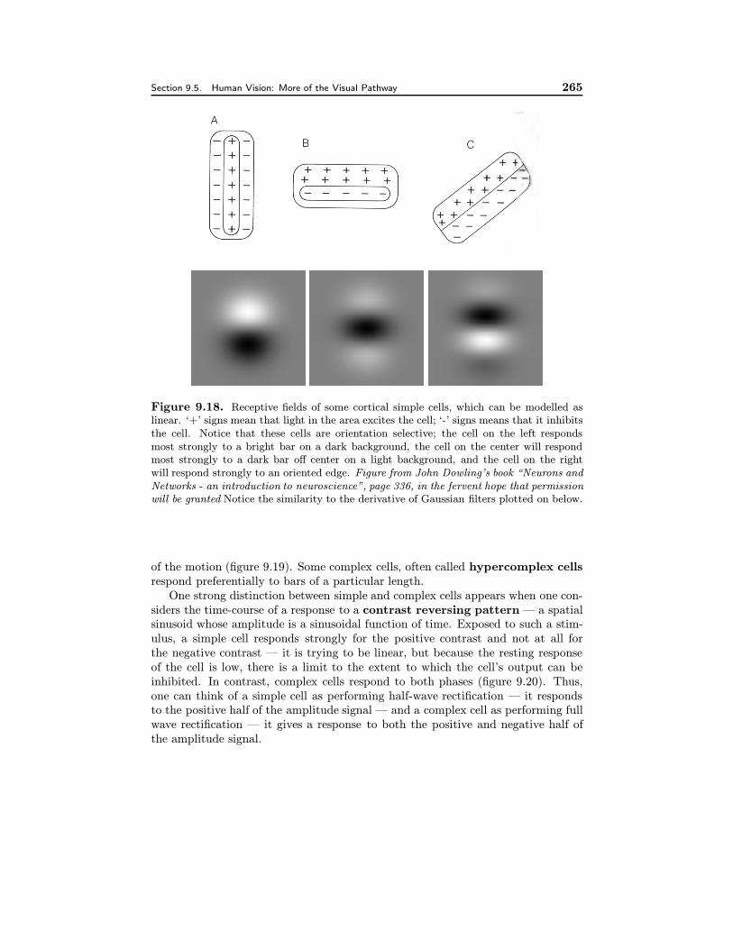
Figure 9.19. Cortical cells give stronger or weaker responses to moving bars, dependingon the direction in which the bar moves. The figure shows the response of a cell toa moving bar; note that, as the bar moves forward in the direction perpendicular to itsextent, the response is stronger than when the bar moves backward. Similarly, the strengthof the response depends on the orientation of the bar. Figure from Brian Wandell’s book,“Foundations of Vision”, page171, in the fervent hope that permission will be granted afterHubel and Wiesel, 1968.

9.5.3 A Model of Early Spatial Vision

We now have a picture of the early stages of primate vision. The retinal image istransformed into a series of retinotopic maps, each of which contains the output of

Section 9.5. Human Vision: More of the Visual Pathway 267

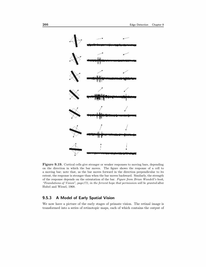
Figure 9.20. Cortical cells are classified simple or complex, depending on their responseto a time-reversing grating. In a simple cell (on the left), the response grows as theintensity of the grating grows, and then falls off as the contrast of the grating reverses.The negative response is weak, because the cell’s resting output is low so that it cannotcode much inhibition. The response is what one would expect from a linear system witha lower threshold on its response. On the right, the response of a complex cell, whichlooks like full wave rectification; the cell responds similarly to a grating with positive andreversed contrast. Figure from Brian Wandell’s book, “Foundations of Vision”, page172,in the fervent hope that permission will be granted after DeValois et al 82

a linear filter which may have spatial or spatio-temporal support. The retinotopicstructure means that each map can be thought of as an image which is filteredversion of the retinal image. The filters themselves are oriented filters that lookrather a lot like various derivatives of a Gaussian, at various orientations. Theretinotopic maps are subjected to some form of non-linearity (to get the output ofthe complex cells).

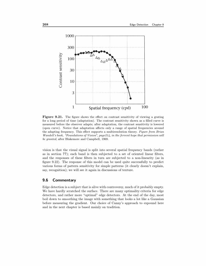
This model can be refined somewhat, with the aid of psychophysical studiesof adaptation. Adaptation is a term that is used fairly flexibly; generally, the re-sponse of an observer to a stimulus declines if the stimulus is maintained and staysdepressed for some time afterwards. Adaptation can be used to determine com-ponents of a signal that are coded differently — or follow different psychophysicalchannels, in the jargon — if we adopt the model that channels adapt indepen-dently. Observer sensitivity to gratings can be measured by the contrast sensi-tivity function, which codes the contrast that a periodic signal must have with aconstant background before it is visible (figure ??).

In experiments by Blakemore and Campbell [], observers were shown spatialfrequency gratings until they are adapted to that spatial frequency. It turns outthat the observer’s contrast sensitivity is decreased for a range of spatial frequenciesaround the adapting frequency. This suggests that the observer is sensitive toseveral spatial frequency channels; the contrast sensitivity function can be seen asa superposition of several contrast sensitivity functions, one for each channel.

This is a multiresolution model. The current best model of human early


Figure 9.21. The figure shows the effect on contrast sensitivity of viewing a gratingfor a long period of time (adaptation). The contrast sensitivity shown as a filled curve ismeasured before the observer adapts; after adaptation, the contrast sensitivity is lowered(open curve). Notice that adaptation affects only a range of spatial frequencies aroundthe adapting frequency. This effect supports a multiresolution theory. Figure from BrianWandell’s book, “Foundations of Vision”, page214, in the fervent hope that permission willbe granted, after Blakemore and Campbell, 1969.

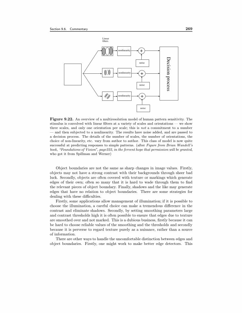
vision is that the visual signal is split into several spatial frequency bands (ratheras in section ??); each band is then subjected to a set of oriented linear filters,and the responses of these filters in turn are subjected to a non-linearity (as infigure 9.22). The response of this model can be used quite successfully to predictvarious forms of pattern sensitivity for simple patterns (it clearly doesn’t explain,say, recognition); we will see it again in discussions of texture.

9.6 Commentary

Edge detection is a subject that is alive with controversy, much of it probably empty.We have hardly scratched the surface. There are many optimality criteria for edgedetectors, and rather more “optimal” edge detectors. At the end of the day, mostboil down to smoothing the image with something that looks a lot like a Gaussianbefore measuring the gradient. Our choice of Canny’s approach to expound hereand in the next chapter is based mainly on tradition.

Section 9.6. Commentary 269

+

noise

+

noise

+

noise

Decision process

nonlinearity

nonlinearity

nonlinearity

Linearfilters

Figure 9.22. An overview of a multiresolution model of human pattern sensitivity. Thestimulus is convolved with linear filters at a variety of scales and orientations — we showthree scales, and only one orientation per scale; this is not a commitment to a number— and then subjected to a nonlinearity. The results have noise added, and are passed toa decision process. The details of the number of scales, the number of orientations, thechoice of non-linearity, etc. vary from author to author. This class of model is now quitesuccessful at predicting responses to simple patterns. (after Figure from Brian Wandell’sbook, “Foundations of Vision”, page222, in the fervent hope that permission will be granted,who got it from Spillman and Werner)

Object boundaries are not the same as sharp changes in image values. Firstly,objects may not have a strong contrast with their backgrounds through sheer badluck. Secondly, objects are often covered with texture or markings which generateedges of their own; often so many that it is hard to wade through them to findthe relevant pieces of object boundary. Finally, shadows and the like may generateedges that have no relation to object boundaries. There are some strategies fordealing with these difficulties.

Firstly, some applications allow management of illumination; if it is possible tochoose the illumination, a careful choice can make a tremendous difference in thecontrast and eliminate shadows. Secondly, by setting smoothing parameters largeand contrast thresholds high it is often possible to ensure that edges due to textureare smoothed over and not marked. This is a dubious business, firstly because it canbe hard to choose reliable values of the smoothing and the thresholds and secondlybecause it is perverse to regard texture purely as a nuisance, rather than a sourceof information.

There are other ways to handle the uncomfortable distinction between edges andobject boundaries. Firstly, one might work to make better edge detectors. This


approach is the root of a huge literature, dealing with matters like localisation,corner topology and the like. We incline to the view that returns are diminishingrather sharply in this endeavour.

Secondly, one might deny the usefulness of edge detection entirely. This ap-proach is rooted in the observation that some stages of edge detection, particularlynon-maximum suppression, discard information that is awfully difficult to retrievelater on. This is because a hard decision — testing against a threshold — has beenmade. Instead, the argument proceeds, one should keep this information around ina “soft” (a propaganda term for probabilistic) way. Attactive as these argumentssound, we are inclined to discount this view because there are currently no practicalmechanisms for handling the volumes of soft information so obtained.

Finally, one might regard this as an issue to be dealt with by overall questions ofsystem architecture — the fatalist view that almost every visual process is going tohave obnoxious features, and the correct approach to this problem is to understandthe integration of visual information well enough to construct vision systems thatare tolerant to this. Although it sweeps a great deal of dust under the carpet —precisely how does one construct such architectures? — we find this approach mostattractive and will discuss it again and again.

All edge detectors behave badly at corners; only the details vary. This hasresulted in two lively strands in the literature (i - what goes wrong; ii - what to doabout it). There are a variety of quite sophisticated corner detectors, mainly becausecorners make quite good point features for correspondence algorithms supportingsuch activities as stereopsis, reconstruction or structure from motion. This hasled to quite detailed practical knowledge of the localisation properties of cornerdetectors (e.g. []).

A variety of other forms of edge are quite common, however. The most com-monly cited example is the roof edge, which can result from the effects of inter-reflections (figure 3.17). Another example that also results from interreflections isa composite of a step and a roof (figure ??). It is possible to find these phenomenaby using essentially the same steps as outlined above (find an “optimal” filter, anddo non-maximum suppression on its outputs). In practice, this is seldom done.There appear to be two reasons. Firstly, there is no comfortable basis in theory(or practice) for the models that are adopted — what particular composite edgesare worth looking for? the current answer — those for which optimal filters arereasonably easy to derive — is most unsatisfactory. Secondly, the semantics of roofedges and more complex composite edges is even vaguer than that of step edges —there is little notion of what one would do with roof edge once it had been found.

Edges are poorly defined and usually hard to detect, but one can solve problemswith the output of an edge detector. Roof edges are similarly poorly defined andsimilarly hard to detect; we have never seen problems solved with the output ofa roof edge detector. The real difficulty here is that there seems to be no reliablemechanism for predicting, in advance, what will be worth detecting. We will scratchthe surface of this very difficult problem in section ??.

Section 9.6. Commentary 271

Assignments

Exercises

1. Show that forming unweighted local averages — which yields an operation ofthe form

Rij =1

(2k + 1)2

u=i+k∑u=i−k

v=j+k∑v=j−k

Fuv

is a convolution. What is the kernel of this convolution?

2. Write E0 for an image that consists of all zeros, with a single one at the center.Show that convolving this image with the kernel

Hij =1

2πσ2exp

(−((i− k − 1)2 + (j − k − 1)2)

2σ2

)

(which is a discretised Gaussian) yields a circularly symmetric fuzzy blob.

3. Show that convolving an image with a discrete, separable 2D filter kernel isequivalent to convolving with two 1D filter kernels. Estimate the number ofoperations saved for an NxN image and a 2k + 1× 2k + 1 kernel.

4. We said “One diagnostic for a large gradient magnitude is a zero of a “secondderivative” at a point where the gradient is large. A sensible 2D analogue tothe 1D second derivative must be rotationally invariant” in section 8.6. Whyis this true?

5. Each pixel value in 500 × 500 pixel image I is an independent normally dis-tributed random variable with zero mean and standard deviation one. Esti-mate the number of pixels that where the absolute value of the x derivative,estimated by forward differences (i.e. |Ii+1,j − Ii,j| is greater than 3.

6. Each pixel value in 500 × 500 pixel image I is an independent normally dis-tributed random variable with zero mean and standard deviation one. I isconvolved with the 2k + 1× 2k + 1 kernel G. What is the covariance of pixelvalues in the result? (There are two ways to do this; on a case-by-case basis —e.g. at points that are greater than 2k+1 apart in either the x or y direction,the values are clearly independent — or in one fell swoop. Don’t worry aboutthe pixel values at the boundary.)

7. For a set with 2k+1 elements, the median is the k+1’th element of the sortedset of values. For a set with 2k elements, the median is the average of thek and the k + 1’th element of the sorted set. Show that it does not matterwhether the set is sorted in increasing or decreasing order.

8. Assume that we wish to remove salt-and-pepper noise from a uniform back-ground. Show that up to half of the elements in the neighbourhood could benoise values and a median filter would still give the same (correct) answer.


Programming Assignments

• One way to obtain a Gaussian kernel is to convolve a constant kernel withitself, many times. Compare this strategy with evaluating a Gaussian kernel.

1. How many repeated convolutions will you need to get a reasonable ap-proximation? (you will need to establish what a reasonable approxi-mation is; you might plot the quality of the approximation against thenumber of repeated convolutions).

2. Are there any benefits that can be obtained like this? (hint: not everycomputer comes with an FPU)

• Why is it necessary to check that the gradient magnitude is large at zerocrossings of the Laplacian of an image? Demonstrate a series of edges forwhich this test is significant.

• The Laplacian of a Gaussian looks similar to the difference between two Gaus-sians at different scales. Compare these two kernels for various values of thetwo scales — which choices give a good approximation? How significant is theapproximation error in edge finding using a zero-crossing approach?

• Obtain an implementation of Canny’s edge detector (you could try the visionhome page at http://www.somewhereorother) and make a series of imagesindicating the effects of scale and contrast thresholds on the edges that aredetected. How easy is it to set up the edge detector to mark only objectboundaries? Can you think of applications where this would be easy?

• It is quite easy to defeat hysteresis in edge detectors that implement it —essentially, one sets the lower and higher thresholds to have the same value.Use this trick to compare the behaviour of an edge detector with and withouthysteresis. There are a variety of issues to look at:

1. What are you trying to do with the edge detector output? it is sometimesvery helpful to have linked chains of edge points — does hysteresis helpsignificantly here?

2. Noise suppression: we often wish to force edge detectors to ignore someedge points and mark others. One diagnostic that an edge is useful ishigh contrast (it is by no means reliable). How reliably can you usehysteresis to suppress low contrast edges without breaking high contrastedges?

• Build a normalised correlation matcher. The hand finding application is anice one, but another may occur to you.

1. How reliable is it?

2. How many different patterns can you tell apart in practice?

3. How sensitive is it to illumination variations? shadows? occlusion?

Chapter 10

NON-LINEAR FILTERS

10.1 Filters as Templates

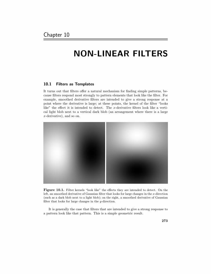
It turns out that filters offer a natural mechanism for finding simple patterns, be-cause filters respond most strongly to pattern elements that look like the filter. Forexample, smoothed derivative filters are intended to give a strong response at apoint where the derivative is large; at these points, the kernel of the filter “lookslike” the effect it is intended to detect. The x-derivative filters look like a verti-cal light blob next to a vertical dark blob (an arrangement where there is a largex-derivative), and so on.

Figure 10.1. Filter kernels “look like” the effects they are intended to detect. On theleft, an smoothed derivative of Gaussian filter that looks for large changes in the x-direction(such as a dark blob next to a light blob); on the right, a smoothed derivative of Gaussianfilter that looks for large changes in the y-direction.

It is generally the case that filters that are intended to give a strong response toa pattern look like that pattern. This is a simple geometric result.

273

Documents

9.1 EstimatingDerivativeswithFiniteDiﬀerencesalgebra.sci.csueastbay.edu/~grewe/CS6825/Book_online/edgedetection.pdf · 1/256, 4/256 and 16/256 of the full range of brightness respectively