9-1

9 ADAPTIVE OPTICS

9.1 Overview of GMT Adaptive Optics

9.1.1 Introduction

The primary goal of adaptive optics is the correction of atmospheric blurring to recover images with the diffraction limited beam profile, thus providing the GMT with correspondingly improved sensitivity. The GMT’s large aperture holds the potential of uniquely sharp images, three times sharper than the limit for current 8 m apertures. The resulting unprecedented sensitivity and resolution of the GMT are illustrated by the modeled Hα image in Figure 9-1 of a starburst galaxy at z = 1.4, in a 1 hour, narrow-band exposure at 1.58 μm. Images of this quality and covering 1000 times the area of the 1″ square shown will be obtained even at the Galactic poles, where the probability of finding a suitable guide star remains high. Figure 9-2 shows the GMT beam profile and that of a filled circular aperture of 24.4 m diameter that has the same resolution. High Strehl AO corrected images from GMT in the thermal infrared will realize this ideal profile in practice, with access to most of the sky and with no compromise of the thermal infrared background.

Figure 9-1. (Left) The 40″ square field of the GMT HRCam imager is shown superposed on a deep 2′ square NICMOS field from the HST. Simulated AO correction over this field is made from wavefront measurements of the six laser beacons projected as shown at 35″ radius, and an H = 17 guide star 1′ off axis. (Right) Detail of a 1″ square within the corrected field showing a starburst galaxy at z = 1.4, as it would be detected in an H band image with the 16 mas resolution of the GMT AO system, ten times that of HST. The input was an Hα image of NGC 4038/39. The individual redshifted HII regions were taken to have H magnitude ~24.5. The detector plate scale is 10 mas/pixel. Sky noise is modeled for a 1 hour exposure through a 2.5% filter at the redshifted Hα wavelength. The insert shows the stellar PSF with the same 10 mas pixel size and the projected 40% Strehl ratio for two stars, one saturated, separated by 100 mas. The elongation is due to increased tilt anisoplanatism in the direction of the guide star.

9-2

Figure 9-2. Aberration-free PSFs for the GMT (left) and a filled 24.4 m disc (middle) which has the same FWHM. Scale in arcsec is for 1.65 μm where the FWHM is 14 mas. Cuts through the radially averaged PSFs are shown on the right, along with the Airy pattern of the individual 8.4 m segments, in a log intensity plot.

9.1.2 Goals for the GMT AO System

The promise of an extremely large telescope (ELT) with AO, combining sharper resolution at the diffraction limit with a huge collecting area, is obvious. But the degree to which adaptive optics at an ELT can deliver on this promise has to be carefully thought through. Our expectation is that not only can higher resolution be achieved, but that a Strehl ratio of 40% can be maintained for H band images, even when the guide star is 1′ off axis for images at the Galactic poles. The GMT’s large aperture gives inherently better sky access; thus adaptive correction will be a powerful tool for the general observer.

The first major step toward increasing sky coverage is now being taken with the development of laser guide stars on 8-m class telescopes. Light from a sodium resonance beacon generated at ~90 km altitude follows the path taken by light from the target closely enough that a good estimate of the aberrations in the latter can be derived. A field star is still needed to measure the fast tip-tilt component of the atmospheric turbulence, but this star can be fainter and further away than if it were needed for measurement of the full wavefront. The power of sodium beacons for science programs is now being realized at the Keck II telescope (Wizinowich et al. 2006).

Laser wavefront sensing can be extended to larger apertures provided the cone effect, which causes a discrepancy between the wavefront of a laser guide star and that of a natural star, can be overcome. This effect increases with telescope diameter and for apertures beyond about 10 m becomes severe. However, for the GMT at 25 m aperture, this problem will be overcome by using six sodium lasers projected in a small-angle constellation from a common launch telescope. A tomographic solution for the turbulence then can be expected to correct the wavefront to the same accuracy or better than an 8 m telescope with a single beacon, in a technique called laser tomography adaptive optics (LTAO).

The sky coverage is potentially better than for the 8 m system for two reasons. One is that the anisoplanatic error in tip-tilt measurement made from a field star at given radius decreases with aperture, even faster than the decrease in diffraction width. As we show below in Section 9.6.7.2, for typical atmospheric conditions, the RMS differential motion projected for the diffraction limited GMT rises to only ~5 milliarcseconds (mas) RMS for a field star at 1′ radius. The second is that the limiting magnitude for useful field stars increases sharply with aperture,

9-3

provided the tilt sensor is built to sense the diffraction core of the star’s laser-sharpened infrared image, rather than a seeing limited optical image (Angel 1992). Not only does the sharpness of the image compared to the seeing limit dramatically improve the sensitivity of the tilt measurement, but by enabling a sensor with pixels of very small angular subtense, the contamination by sky background can be reduced by many magnitudes. In Section 9.4.3.2 we show that the limiting magnitude for tip-tilt sensing with the GMT is ≥17 in the H band, which is the key factor in realizing access to most of the sky. Taken together, we see that with its multi beacon system the GMT should be able to observe most scientific targets, with a contribution to the image width from image jitter of only ~10 mas RMS.

This limit has helped us decide how aggressively we should set GMT goals for wavefront correction with the laser beacon system. Table 9-1 lists the image FWHM at the diffraction limit of the GMT. The H band limit is 14 mas, which would be increased to 17 mas by 10 mas of tilt broadening. In the J band, 11 mas would be increased to 15 mas. Thus in terms pushing the resolution limit for faint objects, we reach a point of diminishing returns somewhere around the H band.

Table 9-1. Diffraction limited image goal for GMT laser system, with 200 nm RMS residual wavefront error.

λ (μm) FWHM (arcsec)

Isoplanatic angle (arcsec)

Strehl (percent)

0.9 0.008 4.2 14 1.25 0.011 6.3 36 1.65 0.014 8.8 56 2.2 0.019 12.4 72 3.5 0.029 21.7 90 5 0.042 33.3 94 10 0.085 76.5 98 20 0.170 176 99.6

The other key factor that must guide us is the corrected field of view. With a single deformable mirror this is limited because the turbulence causing seeing is present at heights up to 15 km, so wavefront aberration varies with viewing angle. The third column of Table 9-1 gives the isoplanatic angle, the nominal field radius in average seeing at which the Strehl ratio drops to 50%, as a function of wavelength, supposing that the on-axis wavefront is perfectly corrected with a deformable mirror conjugated to the telescope pupil. (We note that the isoplanatic angle is as variable as the seeing width, so larger, as well as smaller, values may sometimes prevail).

The corrected field can be increased with multi-conjugate adaptive optics (MCAO), but even with just one deformable mirror, the field in the K band is already 25″ in diameter, and often larger, 1300 times the diffraction width. The H band field of 18″ is similarly rich. The ability to guide on very faint field stars ensures high sky coverage. Thus, MCAO is not included in the baseline design for GMT. The tomographic solution derived from the multiple LGS signals will be used to drive just GMT’s adaptive secondary mirror in the LTAO mode.

These considerations have led us to adopt for the GMT a baseline AO capability with a sodium laser beacon constellation system aimed at good correction in the H band, with near full sky

9-4

coverage. The wavefront correction, at least to start with, will be made with a single common deformable mirror conjugated to the ground turbulence. The target for wavefront correction accuracy from the beacon system is 200 nm RMS under typical seeing conditions. This is chosen to give relatively good Strehl in the H band, 56% for a guide star on axis, degrading to 35% for a tilt star 1′ off axis. The 200 nm RMS target is significantly better than is typically achieved with current systems, but our analysis later in this chapter shows it will be possible. Table 9-1 shows the corresponding on-axis Strehl ratios for other wavelengths.

A second major goal for the GMT is extreme adaptive optics or ExAO, for imaging other solar systems at high contrast. In many cases the targets will be bright, consistent with the more accurate wavefront sensing and correction that will be essential for high contrast. Many targets with known planets are as bright as 6th magnitude, where we can aim at high Strehl correction in the H band. Here, planet imaging to an inner working angle of 4 λ/D (56 mas) is targeted, to allow detection in reflected light of many planets of known mass from radial velocity searches. Correction with AO to 112 nm RMS has been achieved in practice for a star of 6th magnitude in V (Fugate et al. 1999). For the GMT we set a target of 120 nm RMS error for such bright stars, corresponding to 80% Strehl at 1.65 µm. Detection of thermal emission in the M band, where giant planets are expected to be anomalously bright will also be important. Here 120 nm RMS corresponds to 98% Strehl, a level that will allow high sensitivity to ~2 λ/D, or 84 mas radius.

The third goal for AO at the GMT is to improve seeing over a wide field by correction of just the ground layer (GLAO). This method is expected to give useful improvement in the H and K bands over fields up to 10′, and is planned for 8 m telescopes. While the GMT has no qualitative gain over an 8 m telescope in resolution in this mode, GLAO is needed to preserve its quantitative advantage of seven times higher throughput than 8 m apertures. The same laser beacons used for diffraction limited imaging will also serve to implement GLAO simply by expanding the diameter of the beacon constellation and the projected pattern of the corresponding wavefront sensors. The large segment size of the GMT simplifies GLAO in that the individual 8 m apertures have diffraction limits much smaller than the near IR seeing and thus in this mode do not need to be coherently phased.

9.1.3 GMT AO Challenges - Special Considerations for Very Large Aperture

We recognize at the outset that our goals represent both a quantitative leap in resolution compared to ~8 m aperture, as well as a qualitative leap in the art and technology of adaptive optics. The use of laser guide stars for wavefront sensing is a technique still in its infancy with just one laser. Use of a constellation of several laser beacons, with tomographic wavefront sensing in a closed-loop servo is a technique still unproven at any telescope. Similarly, ground layer correction remains a plausible, but still theoretical concept. Very high contrast imaging for exoplanet searches is similarly in its infancy with current telescopes. Thus we are faced with designing AO for a 25 m aperture with operational modes not yet developed even for an 8 m aperture.

To build a telescope that is to be at the forefront in adaptive optics not only ten years hence, but through the following decades, we need the clearest vision of not only its potential as set by physical limits such as atmospheric turbulence and photon noise limited sensors, but also of engineering solutions that can exploit the advanced technology likely to be available then.

9-5

In many instances the optimum AO solution is likely to require incorporation into the GMT telescope itself, rather than development of some black box later. Thus an overriding consideration in designing the GMT has been to try to anticipate these features and build them in. We have built on our AO developments and experience for 8 m class telescopes to provide integrated adaptive optics to the GMT. The critical new technology is that required to combine the seven 8 m wavefront segments into a coherent whole after the segments are individually corrected by methods already known and being developed. We examine here some specific issues peculiar to aberrations across very large apertures.

1) The amplitude of Kolmogorov turbulence increases as the 5/6 power of the aperture, while the wavefront error to reach a given Strehl ratio, after correction, remains independent of aperture. Therefore, there is a new challenge in dealing with unprecedentedly large aberrations of many μm over large scales. These aberrations must be measured and corrected to the same limit of ~100 nm RMS as for small-scale errors. The outer scale of atmospheric turbulence is likely to be approximately equal to the 25 m aperture of the telescope and will provide some relief, but only under some conditions.

2) Wavefront aberrations generated in the telescope itself, from wind-induced vibrations and from local convection, are likely to be larger than for lighter and stiffer small telescopes unless great care is taken.

3) Wavefront discontinuities are present because of segmentation. Fortunately the advances made with the Keck telescope AO system show that the difficulties presented by segmented primaries can be overcome (Wizinowich et al. 2004).

4) The diffraction limit for the thermal infrared for 25 m aperture becomes much sharper than the seeing limit, and so AO correction will enable higher resolution improvement compared to current 6-10 m telescopes. Current large aperture telescopes can be corrected in the 8-12 µm region with a relatively simple tip-tilt secondary unless high dynamic range imaging is important (Close et al. 2003, Liu et al. 2005). But for the GMT the larger aperture with adaptive correction opens the possibility of greatly increased sensitivity in the thermal infrared, provided the advantage of sharper images is not offset by increased thermal background in the AO correction system.

9.1.4 Meeting the Challenges

9.1.4.1 Correction with a Deformable Gregorian Secondary

In order to meet the goals and challenges above, the GMT will base its AO system around a deformable secondary mirror for wavefront correction. There are several advantages:

1) Deformable secondary technology has now matured to the point where it offers excellent overall performance in terms of high stroke and spatial resolution correction, fast response and accurate internal metrology.

2) Since all the telescope foci follow the secondary mirror, atmospheric correction at that mirror will be available for any instrument on the telescope which can benefit and for which wavefront information is available.

9-6

3) Sensitivity at wavelengths longward of ~2 µm is maximized because the correction is accomplished without the conventional addition of warm reimaging optics, a tip-tilt mirror and a separate deformable mirror, all of which contribute thermal background. The deformable secondary mirror will allow diffraction-limited imaging with the highest sensitivity over the full 2-25 µm wavelength range where background emission from separate AO optics could otherwise dominate.

4) For ground layer correction there are two advantages. First the field of view limitations from an optical relay are avoided. Second, the Gregorian deformable secondary conjugates to a height centered on the ground turbulence, 200 m above ground, for the widest possible field.

5) With such a powerful correcting element built-in, the goal of a universal wavefront sensing system becomes practical.

The GMT deformable secondary will be built using the technology developed with the pioneering secondaries built for the MMT (Wildi et al. 2002) and LBT (Riccardi et al. 2004). It is specified to have 4620 actuators, the same number per 8 m segment as for the LBT, and corresponding to a spacing of 32 cm at the entrance pupil. This enables a system with 120 nm RMS wavefront error as desired for ExAO at near and mid infrared wavelengths. It also opens the possibility of correction with useful Strehl ratio at wavelengths significantly less than 1 μm, where very high resolution imaging (~7 mas) around bright targets will be possible with CCD detectors.

9.1.4.2 Conjugated Segments for the Primary and Secondary

We have already mentioned that a new and important task for the GMT AO system is to ensure that the wavefronts from the seven 8.4 m segments are joined together coherently so as to make a single, diffraction-limited whole. The “conventional” approach for a segmented primary telescope, as implemented at the Keck and planned for the JWST, is to use primary actuators to maintain the segment surfaces in exact registration, to avoid edge discontinuities in the wavefront reflected by the primary. For the GMT with its primary of very large segments and a very short focal length, another avenue presents itself, if the deformable secondary is made with the same seven segment configuration as the primary. The task of recovering a continuous wavefront can then be efficiently divided between the two mirrors. This is the route we have chosen. It has the advantage that the highly agile secondary segments can much more readily compensate dynamic disturbances in piston and tilt from the atmospheric turbulence or wind. Thus discontinuities produced by wind gusts will be sensed mechanically between the primary segments but corrected by pistoning the secondary segments. Also by sky baffling each of the secondary segments, the entire complex entrance pupil can be sky baffled, as shown in Figure 9-3. This is desirable to minimize thermal emission, and allows full advantage to be taken of the low emissivity of the two mirror AO corrected system.

9.1.4.3 Constellation of Six Sodium Laser Beacons

To cover all the needs from narrow-field tomography to wide-field ground layer correction, a sodium beacon projection system will be built in to provide a constellation of variable diameter,

9-7

from 1′ to 8′. The diameter will be chosen according to the field to be corrected and the prevailing vertical distribution of aberrating layers. For narrow field tomography, the diameter will be 1.2′, so that their light collectively samples the full volume of atmosphere traversed by light from a target on axis. The instantaneous stellar wavefront will be computed by a tomographic algorithm applied to the wavefronts measured from all the beacons (Ragazzoni et al. 1999, Tokovinin et al. 2001, Lloyd-Hart & Milton 2003). This method will recover the full wavefront across the 25 m aperture. While in the first light configuration correction will be made with the adaptive secondary alone, the tomographic method will yield the information needed to implement multi-conjugate correction (MCAO) for wider field. Thus, the groundwork is laid for this addition at a later stage.

Six beacons will be projected in a regular hexagon. This number is favorable for the tomographic solution, and also for the reduction of interference of the Rayleigh scattered column of one laser with the resonance scattered beacon of another (fratricide). This is markedly reduced if the beacons are projected in the directions of the six gaps, as shown in Section 9.5. Six continuous wave (CW) sodium lasers of 30 W each will be used, based on the existing summed frequency YAG technology demonstrated for guide stars at the Starfire Optical Range (Fugate et al. 2004).

Figure 9-3. Segmented adaptive secondary seen against the sky from the Gregorian focus.

9.1.4.4 Universal Wavefront Sensing Capability

The GMT AO system will provide for simultaneous sensing of the same natural guide star with different sensors at optical and infrared wavelengths, as well as the laser guide stars. The system separates the light between the science instruments and the wavefront sensors by both wavelength division using dichroic mirrors, and by focal plane division with articulated probes to pick off guide stars when the sensing and science need the same wavelength bands. All the sensors will operate across the full pupil, not individual segments.

9.1.4.5 Advanced Natural Guide Star Wavefront Sensors

Our strategy for sensing wavefront aberrations with natural guide stars goes beyond present practice: currently the near-universal choice for AO wavefront sensors are either Shack-Hartmann sensors with CCDs or curvature sensors with avalanche diodes, both working in the visible band. Shack-Hartmann sensors remain the best choice for the beacon wavefront sensors. For very large apertures alternative infrared sensors that can exploit the spatial coherence of

9-8

natural starlight have fundamental advantages. As we have already mentioned, the most valuable of these advantages is for global tip-tilt sensing, in the case where correction by laser guide stars alone has produced instantaneous diffraction limited infrared images of moderate Strehl. Image motion must be measured with a natural star and corrected to ~1/10 the diffraction width to avoid significant reduction in Strehl. This requires detection of around 50 photons in the diffraction limited core. But the photon flux within the core is directly proportional to the telescope collecting area, so for measurement in a given short time interval, the bigger the telescope the fainter star it can work with. This is why the larger telescope has a higher probability of finding a suitable infrared guide star within the isoplanatic angle for tilt.

A unique role for segmented mirror telescopes played by infrared guide stars is to measure the absolute size of steps in the wavefront between the segments, so the edge sensors can be calibrated correctly. The methods developed for the Keck telescope use this principle (Chanan & Pinto 2004) but can be simplified and made more sensitive because of the small number of segments in the GMT.

Infrared wavefront sensors that take advantage of diffraction limited natural star images to measure the full wavefront aberration to high accuracy are also planned. Interferometric wavefront sensors of this type are commonly used in lab metrology systems, but as yet have no track record in astronomical adaptive optics. This is largely because infrared detector arrays with the required high frame rate and sensitivity are as yet unavailable. The VLT has the first IR wavefront sensor (Gendron et al. 2003), but it is a Shack-Hartmann type that does not exploit large scale coherence. Closed loop optical AO systems that exploit full-aperture diffraction have been demonstrated: the fixed pyramid sensor (Esposito et al. 2003), and interferometers that use starlight from the diffraction peak as a phase reference beam (Angel 1994, Colucci & Angel 1992, Codona et al. 2006). PYRAMIR (Costa et al. 2004) will be the first to be used in a closed loop system at the telescope.

The first IR arrays with multiple outputs suitable for such sensing at the GMT are now being developed for use in AO and interferometry. With read noise projected at <10 e- RMS, these would already enable high accuracy IR wavefront sensing of bright stars at the GMT. For ExAO at the highest contrast levels, focal plane wavefront sensors with photon counting infrared arrays are required. We can already plan on small fiber-fed arrays of discrete transition edge infrared photon counting sensors, adequate for searches near the inner working distance. With appropriate investment, larger arrays could be developed in time for the GMT.

9.1.5 AO System Architecture and First Operational Modes

A simple conclusion to be drawn is that achieving the limiting capability for AO correction for the GMT, and indeed any ELT, will require a complex system. It follows that this system should not be duplicated for each instrument needing AO-corrected images, but should be implemented only once if possible. A key challenge is therefore to incorporate all the AO correction and sensing elements into the telescope optical path, making the necessary separation of the beam for wavefront sensing without compromising the science instruments. This has been a guiding principle in designing the GMT telescope AO system.

9-9

Figure 9-4. Schematic diagram of the AO system components mounted on the GMT telescope elevation structure (not to scale). Most of the different science instruments and wavefront sensors remain fixed in place and are brought into play via a set of articulated, retractable dichroic mirrors, marked low, middle and high. The optical sensor unit has Shack-Hartmann sensors for the laser beacons and a natural star, and separate NGS tilt sensors. The IR unit includes sensors for tilt and piston for faint field stars and a high resolution pyramid sensor. The IR field passing through the sensor unit is relayed via a cooled Offner relay (shown as a lens), to multiple science cameras.

The overall concept is shown schematically in Figure 9-4. The deformable Gregorian secondary, the beacon projector, and a removable artificial source are mounted at the top of the telescope. The separate optical and infrared wavefront sensing units are located on the upper side of the instrument platform above the direct focus, along with the diffraction-limited AO instruments. Instruments using GLAO are mounted below. The operation of the system is most readily understood by considering the four basic operational configurations, listed in Table 9-2.

9-10

Table 9-2. Operational modes for the AO system.

Legend: NIR = near infrared, NGS = natural guide star, LGS = laser guide star, PRWFS = pyramid wavefront sensor

9.1.5.1 Mode 1: No AO

Included for completeness, this mode uses no adaptive correction. The dichroic mirrors and lower optical sensors retract to allow the full 24′ field to pass unvignetted to the direct Gregorian focus. All the wavefront control is then from the slow active control system.

9.1.5.2 Mode 2: Ground Layer AO (GLAO)

Ground layer AO in the J, H and K bands. The low-lying component of the turbulence contributes a component of wavefront error common to objects over a much wider field of view than the conventional isoplanatic angle. Images will retain the seeing-limited profile imposed by upper altitude seeing, but will show much less morphological change over the corrected field than in conventional diffraction-limited AO. The size of the correctable field depends on the thickness of the ground layer turbulence, and can be several arcminutes.

In this mode, only the low dichroic mirror is inserted to reflect sodium beacon light and optical field stars. It is sized to transmit up to 8′ of field without vignetting. The ground layer aberration is obtained as the average of all the measured beacon wavefronts, which will be spread out to a diameter up to 8′, depending on the thickness of the ground layer and the desired science field and degree of compensation. The wavefront is corrected by the deformable secondary mirror, which is well conjugated to the ground layer. Because the GMT primary segments are very large, their individual diffraction profiles are smaller than the GLAO images, and therefore it is not necessary to phase them. Thus only tip-tilt and slow focus correction are necessary, and these measurements are provided by up to three field stars sensed with optical probes that range over the 8′ optical field in regions clear of the pattern of six beacons.

9.1.5.3 Modes 3 and 4: Diffraction Limited AO

A plan view of the instrument configuration is shown in Figure 9-5. The near infrared beam for instruments and wavefront sensors operating in the JHK bands is reflected (to the left) out of the main beam by the middle dichroic mirror which transmits optical light through to the low dichroic and optical wavefront sensor. At the bent Gregorian focus a faint natural star will be

Wavefront sensors

Operating mode Science λ (μm)

Focal station

Field (′)

Dichroics: low middle high

Fast tilt and piston

High order

Direct 24 1. No AO - Folded 4 out-out-out - -

2. Ground Layer AO 0.9-2.5 Direct 8 in-out-out Optical NGS LGS 3a. NIR NGS PRWFS 3b. NIR LTAO 0.9-2.5 Folded 1 in-in-out NIR NGS LGS 4a. Thermal IR NGS PRWFS 4b. Thermal IR LTAO

3-25 Folded 4 in-in-in NIR NGS LGS

9-11

accessed by one of three field probes to feed sensors with IR detector arrays to measure slow, flexure-induced phase steps between the seven segments, global image motion at full adaptive speed, and focus shifts arising from changes in the mean height of the sodium layer, none of which are well sensed by the lasers. In addition there will be an infrared pyramid sensor for full wavefront sensing, fed either by a small probe mirror or, to access an on-axis bright target, by a dichroic with one of the J, H or K bands.

Figure 9-5. Schematic plan view of the instrument platform. The thick red arrows show three simultaneous beams going from the low dichroic to the optical sensor (6 o’clock), from the mid-dichroic to the near IR wavefront sensors, Offner relay and instrument, (9 o’clock) and from the high dichroic to a thermal IR instrument (2 o’clock). HRCAM allows NIR (1-2.5 μm) AO imaging and long slit spectra. The ExAOCAM allows very high-contrast NIR imaging. NIRS allows very high resolution spectra from 1-2.5 μm (SWM) and 3-5 μm (LWM). MIISE allows 3-25 μm imaging, spectra, and nulling. See Chapter 13 for more detail on each of these AO instruments.

The full suite of optical and infrared sensors can be used to correct for science instruments both in the JHK bands, which would access the 1′ field passing the sensors and corrected by an Offner relay (mode 3), shown in Figure 9-6, and in longer thermal bands, feed a 4′ field by reflection from the high dichroic brought in above, transmitting both optical and near infrared through to the sensors (mode 4). To maintain diffraction limited imaging performance for the near IR sensors when the upper dichroic is in place, aberrations in the transmitted beam will be corrected by a compensating plate inserted ahead of the near IR focus. In all cases the science beam will be correctable either by tomography with laser beacons, or by a natural star in the field.

9-12

Figure 9-6. Configurations for modes 3 and 4, IR diffraction limited imaging (view rotated 90 degrees from Figure 9-5 above). A 4′ field in the thermal IR is reflected to the instruments off the top dichroic, which transmits visible and near IR. For the near IR a dichroic is introduced to reflect a 4′ beam over 1-2.5 μm to the left, while transmitting the optical beam through to the lower dichroic and optical wavefront sensors. This beam enters the dewar before the focus. The infrared sensors deploy across the 4′ field, and a 1′ field passes through to the modified Offner relay which yields an f/15 beam. This passes through an atmospheric dispersion corrector up to a beam steering mirror to the instruments, which are connected by gate valves.

9.1.5.4 Mode 3: 1 to 2.5 µm Diffraction Limited AO

An Offner relay provides science instruments in this mode a 1′ field corrected to the diffraction limit in the J band, and includes an atmospheric dispersion corrector and a cold, rotating pupil stop. The pupil image at this stop is of high fidelity, with only 0.6% anamorphic distortion, thus a rotating stop masking thermal emission outside the seven circular segments will be located here. If required, a fast steering mirror could also be located at this pupil to control non-common path vibration. The relayed beam is at f/15, for a plate scale of ~2 mm/arcsec. Different instruments will be accessed by a steering mirror turning about an axis parallel to the main axis and displaced by 2 m. The diffraction limited FWHM in the K band of 0.019″ will be critically Nyquist sampled in the direct beam by pixels of 16.5 μm.

9.1.5.5 Mode 4: Thermal Infrared Diffraction Limited AO

For instruments operating in the thermal infrared, the high dichroic is added on the main telescope axis, above the first two. It reflects just wavelengths longer than 3 μm and transmits the optical and the near infrared to the wavefront sensors below. This reflection is made with 30° angle of incidence, so as to bring the reflected beam clear of the wide field where it can be folded down to the science instruments within the 2 m clearance above the platform. Because it is not possible to make a single dichroic with high reflectance from 3 to 25 μm and good

Steering mirror and gate valves to mode 3 instruments

Atmospheric dispersion corrector

Rotating cold pupil stop Middle dichroic

transmits optical light to laser WFS

f/15 beam

Infrared tilt and piston and pyramid sensors

2 m

High dichroic inserted for mode 4 thermal IR instruments

9-13

transmission in the near infrared, we plan for interchangeable dichroics. One with a single very high reflectance stack will be used to reflect the L and M bands (3.4-5.1 μm). The second of thin gold has high reflection at wavelengths 8-25 μm and transmits the optical and J bands through to the wavefront sensors. Details are given in Section 9.8 below.

9.1.5.6 Extreme Contrast AO

Instruments for extreme contrast (ExAO) imaging will operate in both the near (HRCAM, ExAOCAM) and thermal (MIISE) infrared positions, and will benefit from the clean and simple optics of the telescope's AO system. Most if not all of the needed wavefront correction can be provided by the deformable secondary. The telescope’s high resolution IR wavefront sensor will be used also, though for the brighter stars additional focal plane interferometric wavefront sensors will likely be incorporated in ExAOCAM. High contrast imaging of fainter stars such as late M stars, brown and white dwarfs will still benefit from laser tomography to allow imaging at extreme contrast ratio. A key requirement for the GMT discussed later in this chapter is a way to suppress the complex diffraction PSF of the seven-segment pupil close to the star.

9.1.5.7 Future Advanced AO Modes

The initial system with its multiple laser beacons and tomographic analysis lays the groundwork for multi-conjugate and multi-object AO (MCAO, MOAO) (Beckers 1988, Tokovinin et al. 2000, Dekany et al. 2004). These techniques complement the 3D tomographic wavefront solution for the atmospheric turbulence with 3D correction involving additional deformable mirrors conjugated to higher altitude. In this way correction to the near IR diffraction limit over a field of 1-2′ should be possible, several times the isoplanatic angle. The GMT design does not call for MCAO or MOAO to be implemented initially, but the AO system, including the lasers, tomographic sensing, and adaptive secondary mirror make a natural base which could readily be extended later on to include them.

9.1.6 Organization of the AO Chapter

The remaining sections of this chapter develop the details of the AO system and its expected performance.

Section 9.2 discusses and summarizes the performance requirements. It includes a definition of common AO terms and a summary of the projected atmospheric characteristics of the Las Campanas site. From these are derived the requirements for the different AO modes, natural guide star, laser tomography (LTAO), thermal imaging, high contrast imaging (ExAO), and ground layer correction (GLAO). The section includes error budgets for the primary modes.

Section 9.3 summarizes research at the University of Arizona in the advanced AO techniques to be used at the GMT. These techniques include: (1) the development of deformable secondaries with Arcetri Observatory, (2) field tests at the MMT of the first multi-beacon system of tomographic and ground layer wavefront sensors, (3) closed loop AO correction of atmospheric piston errors across the old MMT mirrors, and (4) results of lab tests of an AO system closed about an interferometric focal plane wavefront sensor, as planned for ExAO at the GMT.

Section 9.4 describes the strategy for wavefront sensing and control, and gives a detailed

9-14

discussion of the optical and infrared sensors required to provide the initial AO capabilities. Sensitivity estimates are given for natural star sensing of the high order and tilt terms.

Section 9.5 describes the GMT’s sodium laser beacon constellation, with an overview of the chosen multi-beacon geometry optimized for laser tomography, and the optics and mechanics of the laser projection optics.

Section 9.6 covers the GMT AO as a system, including the strategy for bringing the seven 8 m wavefront segments into a diffraction limited whole. System performance estimates are developed, including all error sources that lead to the projected performance in LTAO mode, as illustrated in Figure 9-1.

Section 9.7 describes the real-time wavefront reconstructor.

Section 9.8 describes the optical and mechanical system used to share the telescope beam between the optical and infrared wavefront sensors and the science instruments. It includes details of the dichroics and the Offner relay that provides a corrected f/15 beam to the near IR AO instruments.

9.2 AO Requirements

9.2.1 Some AO definitions

Since some readers will not be familiar with AO jargon, we start with some quick definitions that experts may skip.

Strehl ratio and phase errors. The Strehl ratio S is the ratio of the peak intensity of the aberrated image to that with perfectly flat wavefront. For aberration that is not too large it is given in terms of the RMS wavefront aberration σ (in meters) by the Maréchal approximation S = exp(-2πσ/λ)2 . Here 2πσ/λ is the phase aberration in radians, which is dependent on the wavelength λ. For random aberrations from different sources which add in quadrature we can assign Strehl ratios to the different terms and multiply them to get the system Strehl ratio.

Structure function and rx. The structure function characterizes the wavefront phase aberration in terms of the time-averaged RMS difference in phase between two points as a function of their separation. Kolmogorov turbulence is a good representation of the atmospheric turbulence on scales of 0.1 to a few meters, and in this range the structure function is given by F(Δx) = ⟨[φ(x)-φ(x+Δx)]2⟩ = 6.88(Δx/r0)5/3. Fried’s length r0 is a measure of the seeing. For 1″ seeing at 0.5 μm wavelength r0 = 10 cm.

Outer scale of turbulence L0. Atmospheric turbulence does not keep increasing for scales larger than L0. As a consequence the above structure function overestimates turbulence for scales greater than a few meters. A finite outer scale modifies the power spectrum of phase fluctuations from Φ(κ) α κ-11/3 (Kolmogorov, infinite outer scale) to Φ(κ) α (κ2 + κ0

2)-11/6 (von Karman), where κ is the spatial frequency and κ0 = 2π/L0. This is very significant at the 24.4 m size of the GMT pupil: for a typical observed value of L0 of 25 m, it represents a reduction in power by a factor of 3.4.

9-15

Fitting error. An AO system will not be able to correct errors below some critical length, set by the larger of the actuator spacing on the DM or by the subaperture size of the wavefront sensor. Because this dimension s is small, the fitting error is appropriately derived from the Kolmogorov structure function. The error is given by:

σ fit (nm) = 43 sr0(0.5μm)

⎛

⎝ ⎜

⎞

⎠ ⎟

5 / 6

Equation 9-1

Anisoplanatism and θ0. Wavefront correction applied with a single DM will be correct for an object on axis. The correction will degrade for objects further away in the field. The RMS phase error for an object at angle θ is given by:

σ aniso(nm) = 80 θθ0(0.5μm)

⎛

⎝ ⎜

⎞

⎠ ⎟

5 / 6

Equation 9-2

Tilt and piston anisoplanatism. The anisoplanatic error described above affects all modes of the wavefront. Of particular concern for GMT is the error in global tip-tilt (tilt anisoplanatism) and in the measured mean phase differences between the seven segments (piston anisoplanatism) because these terms must be sensed from a star which will in general be offset from the science target. These terms are dependent on θ0 and L0 and are derived by modeling.

Focus anisoplanatism. Because laser beacons are at finite height in the atmosphere, rays of light from LGS sample the atmosphere differently from rays of starlight. The resulting difference between wavefronts measured from a natural star and those from an LGS pointed in the same direction is called focal anisoplanatism. For 8 m telescopes, the error is not so large as to prevent high Strehl imaging in H and K with a single LGS, but the error grows with aperture, and at the size of GMT the error would be prohibitive with a single LGS.

Servo lag error and τ0. For a correction applied to the wavefront shape at time t based on measurements recorded an interval Δt earlier, the wavefront will have evolved, introducing a phase error given by:

σ time (nm) = 80 Δtτ 0(0.5μm)

⎛

⎝ ⎜

⎞

⎠ ⎟

5 / 6

Equation 9-3

Reconstruction error. Even with noise-free data from hypothetical perfect wavefront sensors, the recovery of the wavefront by the reconstructor computer will be in error. The error depends on the type of sensor used and arises because most sensors do not measure directly the quantity we seek (the wavefront phase aberration) but some related quantity such as the average phase gradient over a subaperture, and information is to some degree inevitably lost in translation. For highest contrast ExAO imaging, interferometric sensors are used to avoid this error.

9-16

9.2.2 Summary of Adopted Atmospheric Parameters

As a baseline for quantifying the atmospheric disturbance and the performance of the AO systems in overcoming it, we have adopted values of the atmospheric parameters describing the spatial coherence r0, temporal coherence τ0, and the isoplanatic angle θ0. In addition, an outer scale of turbulence L0 of 25 m has been assumed. These values have been derived from measurements from several sources: near-continuous night-time monitoring with MASS and DIMM instruments for the full year 2005 at both Cerro Las Campanas at the site of the 6.5 m Magellan telescopes and at Cerro Tololo, and data from balloon flights conducted during the site testing campaign for Gemini South on Cerro Pachón. The values adopted are summarized in Table 9-3 below.

Table 9-3. Adopted values for key atmospheric parameters.

0.5 μm 2.2 μm Parameter Median 10 %ile 90 %ile Median 10 %ile 90 %ile

r0 (cm) 14.3 25.3 9.4 84.6 150 55.6 τ0 (ms) 2.07 3.51 0.79 12.2 20.8 4.7 θ0 (arcsec)* 2.10 2.80 1.33 12.4 16.6 7.9

*Values of θ0 at 2.2 μm do not include the effect of outer scale, which will improve the size of the corrected field of view.

9.2.3 Wavefront Accuracy Requirements for Diffraction Limited Imaging

The initial system will include provision for AO operation for general purpose diffraction limited imaging with maximum sky access, based on wavefront sensing with multiple laser guide stars (LGS) and a highly sensitive infrared tip-tilt sensor. It will also include a simpler system for higher accuracy wavefront correction derived from bright natural stars (NGS).

Performance targets are defined primarily in terms of residual wavefront error in the beam delivered by the telescope to AO instruments. The targeted wavefront errors for the GMT are 200 nm RMS for general purpose LTAO observations, and 120 nm RMS for bright natural guide stars (NGS). These are higher quality than achieved by current AO systems, but we project will be achievable with the GMT. The basis for this expectation comes from analysis of the various component errors which depend on many factors such as telescope aperture, laser power, and detector noise considered in this section and in Sections 9.4 and 9.6 below. Table 9-4 summarizes the performance in terms of Strehl ratio estimated by the Maréchal formula, for on-axis sources in average seeing as given in Table 9-3.

9.2.4 LGS Performance Requirements

Estimates of the performance of 8 m class laser beacon systems have been made since 1994, when Sandler et al. set out the various contributing terms. In that paper a system wavefront error of 310 nm was projected for a tip-tilt guide star on-axis, for somewhat better than the average conditions adopted above (r0 = 18 cm, θ0 = 3″, τ0 = 3.6 ms, all at 500 nm). The largest error contribution was from the fitting error of 180 nm from the assumed 1 m subapertures.

9-17

Table 9-4. Strehl ratio for targeted residual wavefront error.

λ (μm) r0 (cm) τ0 (ms) Strehl (200 nm)

Strehl (120 nm)

0.65 19.6 2.8 0.024 0.26 0.9 29.0 4.2 0.14 0.49 1.25 42.9 6.2 0.36 0.69 1.65 59.9 8.7 0.56 0.81 2.2 84.6 12 0.72 0.89 3.6 153 22 0.88 0.96 5 227 33 0.94 0.98 10 521 75 0.98 0.99 20 1200 173 0.99 1.00

Within the past couple of years, the first system of this type has been realized at the Keck II telescope. A total closed loop system wavefront error of 421 nm RMS was reported for its first engineering runs (Bouchez et al. 2004). It is recognized that many of the contributing factors listed can be improved in the future, including the dominant term of 275 nm RMS from noise in the beacon sensor. This should be reduced by as much as a factor of ten by increased beacon brightness from a non-saturating CW laser. Such lasers with enough power (20-30 W) and in sufficient number are feasible with today’s demonstrated technology (Fugate et al. 2004). The second largest term is focus anisoplanatism, listed for the Keck system at 155 nm, (136 nm for the smaller 8 m aperture of Sandler et al. and intolerably large for the 24.4 m GMT), but this will be mitigated by tomographic reconstruction (LTAO) at the GMT. The third is fitting error at 128 nm, a basic limit set by the Shack-Hartmann subaperture size, which for the Keck is 0.57 m. This error will be 110 nm in the same seeing for the GMT’s 0.49 m subapertures. The fourth term is 110 nm from imperfect measurement of tip-tilt, set by the bandwidth of the tip-tilt star sensor. As we show later, this can be much reduced by use of a fast infrared sensor, but at the GMT will be replaced by tilt anisoplanatism of similar amount for typical field stars 1′ off axis at high Galactic latitude.

Our target of 200 nm RMS for the GMT laser system is aggressive, but is supported by the error budget in Table 9-8 below, by our analysis in Section 9.6, and by numerical simulations by De La Rue & Ellerbroek (2002).

9.2.5 NGS Performance Requirements

The GMT will have two separate wavefront sensing stations, one optical and one infrared. Because the wavelengths are split by a full-field dichroic mirror, both can obtain wavefront data on the same star at the same time.

The initial optical sensor will be a conventional Shack-Hartmann system with a CCD sensor. This will have 0.494 m subapertures configured in the same format as for the LGS sensors. In addition to correcting at high speed in its own right, the optical NGS sensor will be used at low bandwidth in conjunction with the LGS, to guard against focus errors introduced by unknown changes in mean range to the sodium layer, and slowly changing discrepancies between the laser

9-18

and stellar wavefronts. In this mode it will likely work with the optical component of the same off-axis star whose IR flux is being used to measure rapid tip-tilt and slow piston differential.

The infrared sensor will be used in the high accuracy correction system, given a bright star. We set the 120 nm RMS wavefront error requirement to allow very high Strehl and high contrast imaging in the near IR and very high resolution imaging (<10 mas) with useful Strehl down to visible wavelengths. It forms the basis of the high contrast exoplanet imaging system described in Section 9.2.8 below. For the initial infrared sensor we baseline a pyramid sensor, on the assumption that these sensors will be shown to realize in practice their theoretical advantage, and that fast, low noise infrared array detectors with adequate format are developed in the next few years. Subaperture size will be dynamically defined by binning pixels in the sensor’s pupil images, with highest resolution at 0.32 m to match the deformable secondary actuator pitch. At this resolution, for which the fitting error is 84 nm in average seeing (r0 = 14.4 cm), it will be possible to measure and control bright star wavefronts to the 120 nm RMS target.

9.2.6 Additional Requirements for Diffraction Limited AO

9.2.6.1 Corrected Field of View

We do not specify a field of view for the science imaging as a performance requirement, since we do not plan to implement multiconjugate correction for the initial system and the field is thus set by the prevailing atmospheric conditions. The corrected field set by the isoplanatic angle is wavelength dependent, and its radius given by Equation 9-2 is set out in Table 9-1. In practice, larger isoplanatic angles are observed because of the effect of an outer scale of turbulence typically measured to be 25-30 m.

9.2.6.2 AO Instrument Interface

The goal is that all the sensing and control requirements for performance at the required levels are incorporated in the GMT telescope system. Dichroic and field mirrors remove the light needed for the wavefront sensors and segment phasing system. The AO instruments will need only a slow field star guider to remove effects of differential flexure.

9.2.6.3 System Stability

The AO system must hold a stable lock for up to an hour. Non-common path flexure, including the effect of slow guiding on a field star, must be held to no more than 3 mas over any 5° change of elevation angle to preserve image placement on a spectroscopic feed.

9.2.7 Requirements for Thermal AO

9.2.7.1 Thermal Background Emission

The requirement is set that the thermal emissivity of the entire telescope and AO system be less than 7%. This is set by the desire to take advantage of the low thermal background in those regions of the spectrum where sky is especially dark, for example, at 3.8 µm and 11 µm. In these regions the sky background is at or below that of a 3% emissive gray body. Even clean

9-19

telescope optics are expected to contribute at approximately this level, and any unnecessary additional emissivity will result in additional observing time to reach the same sensitivity level.

9.2.7.2 Chopping

The variable nature of the sky background in much of the thermal infrared places a requirement on rapid beam switching or chopping. The majority of observations will be of point source images (<1″) where the throw angle should be significantly larger than the image size. We place a requirement of chopping 20 λ/D full throw at the longest wavelength of observation (25 µm), or a full chop throw of approximately 4″. This is within the range of the deformable secondary’s actuators allowing implementation of chopping with the secondary, as is standard practice for thermal infrared observations.

The rate of chopping should be sufficient to minimize the noise contribution of the variable sky brightness. Our experience with the MMT AO system is that the sky does not vary at rates above 0.1 Hz on good nights. On nights which have thin clouds or high water vapor the sky variation can be both stronger and vary more rapidly. Thus the secondary should chop at least as fast as 1 Hz, with a goal of 5 Hz. The duty cycle should be 90% for this arrangement, requiring transition times of less than 50 ms and 10 ms for the requirement and goal rates respectively.

9.2.8 ExAO Requirements for Imaging Extrasolar Planetary Systems

9.2.8.1 GMT ExAO Goals

The GMT will be used for direct detection of planets in two distinct wavelength regimes: 1.1-2.5 μm (J, H, and K bands) and 3.5-5 μm (L and M bands). In general, shorter wavelengths will allow imaging of planets fainter and closer to their parent star, but the diffraction limit advantage is offset by the difficulty of controlling residual wavefront phase errors and poor planet/star contrast for reflected light detections.

The best candidates for imaging in reflected light are nearby giant planets that are already known to have planets from radial velocity surveys. There are ~10 of them visible from Chile in the radius range 50-100 mas, with contrast ratios projected to cover 1.5–6.5×10-8. They orbit stars with mH = 4–6. Detection of these would be a huge advance over the present state of the art, represented by the detection of AB Dor C at 120 mas at a contrast ratio of 100 in the H band (Close et al. 2005). But it is a challenge we project will be possible to meet with the GMT.

Self luminous hot planets around very young stars may be detectable in the near IR at much larger radii and with less demanding contrast. Thus the nearest young stellar associations may offer easier targets (though still very difficult). Older, cooler planets around more nearby stars will be good targets for detection in the thermal infrared, the most favorable band being at 5 μm, where their contrast is expected to be typically ~10-5 for a 4 MJ planet of age 1 Gy (Burrows et al. 2004). Some of the planets known already at 10 MJ and at orbital radii out to a few AU should be detectable, and there will likely be many more further out with long periods that have escaped RV detection.

9-20

Each of these wavelength regions places a different requirement on the performance of the adaptive optics system, but for both it seems likely that scientific value will be greatest if the AO system will allow very high contrast very close to the star, within a few diffraction widths. Only at these separations will it be possible to study a significant sample of planets of known mass from radial velocity, as well as to probe separations similar to giant planets in our own solar system.

Another area for study of extrasolar systems will be of debris disks, indicative of planetismals. This will also involve both NIR detection (through scattered light) and thermal detection at N band. For the latter the GMT pupil geometry with its large unobscured segments is well suited for nulling interferometry, a method being developed at the LBT (Hinz et al. 2004).

9.2.8.2 Strategy

Our goal with the GMT is to reach the fundamental sensitivity limit for ground based observations set by photon noise in the wavefront sensor when tracking the random component of evolving atmospheric turbulence. If this limit can be reached, sensitivity to at least the 10-8 contrast level could be achieved, as we show below. The principles of such correction are important to understand now, so the architecture of the GMT’s AO system can be built to facilitate this capability. It would be a mistake to build a system that would operate well for normal AO use, but would corrupt the corrected wavefront in some way that would preclude further sensing or correction to very high contrast.

Our expectation is that high contrast imaging will be accomplished by the telescope AO system working in conjunction with specialized ExAO instruments. Ideas for high contrast coronagraphic and interferometric instruments are evolving rapidly, in part because of the activity in developing similar instruments for NASA’s TPF. The instruments will include apodization of the GMT pupil to suppress diffraction, simultaneous imaging in narrow spectral bands that sample across absorption bands (Close et al 2005) and likely also specialized wavefront sensing and an additional very high speed deformable mirror.

9.2.8.3 Requirements for High Contrast Imaging

The desired optimum performance of an AO servo is different for very high contrast imaging than for “normal” AO imaging. For typical adaptive optics based on laser beacons or faint natural guide stars we are concerned with achieving correction of the chaotically-evolving wavefront on the basis of relatively noisy wavefront sensor data. The servo strategy currently used is simply to measure and correct as fast as possible. This maximizes the Strehl ratio, which maximizes the resolution and sensitivity against a sky background that is independent (or nearly so) of the degree of correction. We are not usually concerned about the details of the diffraction pattern, just happy enough to see Airy rings at all.

The situation is different for the bright sources typical of much exoplanet imaging. Since exoplanets will frequently be found in the regions of sky very close to bright stars, the scattered and diffracted starlight halo will generally be the dominant limitation to detection. But the strong photon flux also opens the possibility of high accuracy sensing and correction methods. Thus, our AO imaging system goals are expanded.

9-21

We must make corrections that:

1) Reduce the RMS wavefront error, thereby maximizing the intensity of the exoplanet image,

2) Apodize the beam to suppress diffraction,

3) Minimize the noise in the averaged star halo in the search region,

4) Avoid aliasing and non-common path errors by focal plane sensing and simultaneous differential imaging.

9.2.8.4 Strehl Ratio Requirement

The requirement for high Strehl ratio for high contrast imaging is driven mostly by the need to keep the planet signal as high as possible. We have set our target for 80% Strehl ratio for bright targets in the H band, which translates to 120 nm RMS wavefront error.

A second requirement comes from nulling interferometry in the thermal infrared. The light remaining in the nulled beam can be approximated by taking the amount of uncorrected light (1- S) and dividing it by the actuator count in each nulled beam (the individual 8 m apertures). In order to achieve a 104 null at 11 µm wavelength we require a Strehl ratio of 98%.

9.2.8.5 Apodization of the GMT Pupil

The native PSF for the GMT is more complex than the Airy pattern for a filled disc. In the ideal Airy case 84% of the energy peak is in the central core and 16% in the rings. For the GMT, 66% is in the core and 34% in the wings. (No telescope is ideal – for example, the HST’s performance is scarcely better, 72% in the core and 28% outside). In all cases some form of coronagraph or apodization is therefore needed to give strong diffraction suppression very close to the stellar core. Conventional Lyot coronagraphy is inefficient at best, because strong suppression near the core results in substantial loss of both flux and resolution. This is especially true for the GMT pupil. However, efficient apodization of the GMT pupil close-in is possible. The most efficient method in principle would be that of phase induced amplitude apodization (Guyon 2005). This requires further analysis and optical manufacturing methods that are under development. Here we analyze the use of phase apodization (Codona & Angel 2004), which can be readily implemented. The correction is restricted to a maximum castor of 180° in the focal plane, but has the advantage of high throughput and almost no loss of resolution.

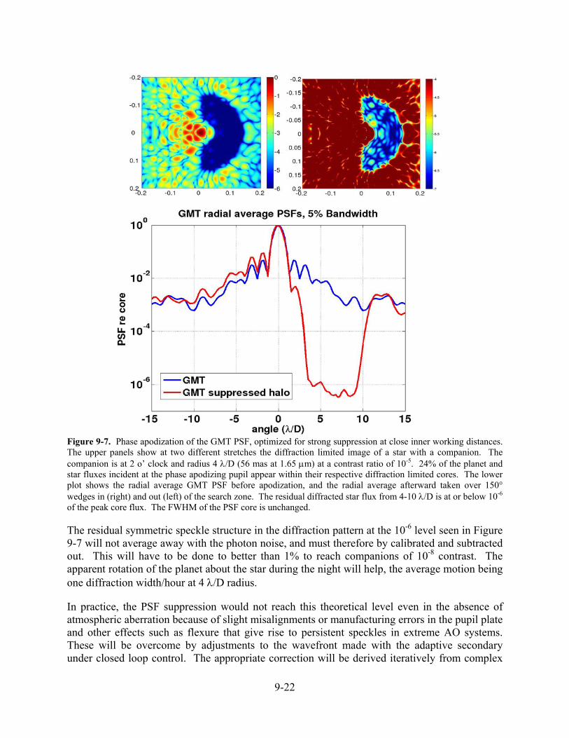
Phase apodization requires introduction of a static phase aberration across the pupil. This will be done in practice with a contoured transmission plate at a pupil stop. The effect is to modify the PSF so as to move energy from one side to the other. The correction is chromatic, but for 5% bandwidth can be very effective, as shown in Figure 9-7, which shows suppression to 10-6 from 4–10 λ/D. We envisage that an ExAO instrument would implement several 5% bandwidth channels used simultaneously, separated by dichroic mirrors. The bands would be imaged simultaneously, with bands chosen in and out of the strongest absorption features.

9-22

Figure 9-7. Phase apodization of the GMT PSF, optimized for strong suppression at close inner working distances. The upper panels show at two different stretches the diffraction limited image of a star with a companion. The companion is at 2 o’ clock and radius 4 λ/D (56 mas at 1.65 μm) at a contrast ratio of 10-5. 24% of the planet and star fluxes incident at the phase apodizing pupil appear within their respective diffraction limited cores. The lower plot shows the radial average GMT PSF before apodization, and the radial average afterward taken over 150° wedges in (right) and out (left) of the search zone. The residual diffracted star flux from 4-10 λ/D is at or below 10-6 of the peak core flux. The FWHM of the PSF core is unchanged.

The residual symmetric speckle structure in the diffraction pattern at the 10-6 level seen in Figure 9-7 will not average away with the photon noise, and must therefore by calibrated and subtracted out. This will have to be done to better than 1% to reach companions of 10-8 contrast. The apparent rotation of the planet about the star during the night will help, the average motion being one diffraction width/hour at 4 λ/D radius.

In practice, the PSF suppression would not reach this theoretical level even in the absence of atmospheric aberration because of slight misalignments or manufacturing errors in the pupil plate and other effects such as flexure that give rise to persistent speckles in extreme AO systems. These will be overcome by adjustments to the wavefront made with the adaptive secondary under closed loop control. The appropriate correction will be derived iteratively from complex

9-23

amplitudes measured interferometrically in the focal plane, thus avoiding all non-common path errors and aliasing effects. (This was the method used to obtain the Airy ring suppression described below in Section 9.3.4). The outer radius of suppression is set by the density of actuators across the deformable mirror. We set as a target control out to 0.6″ radius, which in the H band corresponds to 35 λ/D. This requires 60 actuators across the pupil, or about 35 cm actuator spacing at the entrance pupil.

9.2.8.6 Minimizing the Noise in the Averaged Star Halo Background

Obtaining a stellar halo background that is both faint and smooth requires three different elements: 1) minimizing the photon noise, i.e. the halo intensity in the search region. 2) minimizing the speckle correlation time so that atmospheric speckles will quickly average out in the integrated background and 3) eliminating non-common path wavefront errors that cause unsensed and slowly evolving speckles in the search region.

The halo intensity in the critical search region very close to the star is controlled by errors of low spatial frequency across the pupil, thus for the GMT the strength of the halo at 4 λ/D is set by Fourier terms of wavelength 6 m. The spatial fitting error is not a significant factor in controlling such long wavelengths. Temporal errors are more challenging. These are caused by the lag between the interval needed to collect a useful number of photons for the WFS and the time when the processed information can be applied to the DM. This lag error sets the residual intensity level. The nature of the problem posed by lag is illustrated in Figure 9-8.

Here we have numerically modeled for the phase-apodized GMT pupil the evolution of the complex amplitude at 1 ms intervals at a radius of 4 λ/D, at 9 points in the focal plane shown in the circles in the inset PSF. The atmosphere was modeled with near average conditions of r0 = 15 cm and τ0 = 2.5 ms at 0.5 μm wavelength, as “boiling” turbulence, by superposing several pairs of phase screens moving in opposite directions at 20 m/s. The amplitudes show the evolution assuming that at t = 0 the wavefront is perfectly compensated by an AO system, which is then frozen. They are normalized to the star peak; assuming an observed wavelength of 1.65 μm wavelength, where 4 λ/D is 56 mas. Thus the intensity of a point in the halo with amplitude 0.01 will appear at 10-4 of the stellar core. We find that after 1 ms the amplitude is typically 0.005. Thus a simple servo with 1 ms lag would show instantaneous speckles at 2.5×10-5 of the stellar peak. Because the complex amplitude tracks are mostly linear for a few milliseconds, the error resulting from lag would repeat with about the same value for ~10 ms and thus the speckles would average out only slowly. A companion at 2.5×10-5 of the star would appear the same as a speckle over its 10 ms lifetime, and thus be detected at 1σ in that time. A 104 s integration to reduce speckle noise would thus be required for 5σ detection of a companion at 1.25×10-6.

However, we can expect to do a lot better with a tracking servo, as first pointed out by Stahl and Sandler (1995), because the photon flux from the star is enough to allow accurate complex amplitude measurements on millisecond time scale. The photon count N from a candidate star at H = 5 incident on the telescope pupil in a 1 ms integration is 107. A coherent wavefront sensor with an effective overall efficiency of q = 10% will be able to measure the phase and amplitude of the Fourier components across the wavefront with a normalized amplitude error ~1/√(qN) = 0.001 (Angel 2003). Error bars of this amplitude are drawn in Figure 9-8.

9-24

Figure 9-8. Evolution of the complex amplitude of Fourier components of the wavefront across the GMT pupil that result in starlight diffracted into the 9 points at 4 λ/D radius shown in the inset. The evolution supposes the wavefront is perfectly corrected in phase at t = 0. The plotted points show the complex amplitude normalized to the stellar peak at intervals of 1 ms, computed for λ = 1.65 μm.

If the AO servo is such that at each instant of measurement the amplitudes of the Fourier terms being applied to the DM are known, then their tracks can be reconstructed and a prediction made of the shape change to be applied, as a superposition of the predicted Fourier amplitudes. In this way it would seem possible, given a DM with smooth predictable and known response, and the predictability of low frequency atmospheric evolution shown in Figure 9-8, to significantly reduce both the residual halo intensity and the speckle correlation time by an optimized tracker.

The limit depends on many details of the measurement technique, but for a DM with 0.5 ms response time, and a sensor with 2 kHz frame rate, a limit set by sensor photon noise, we estimate that correction should be achievable to residual amplitudes of 2×10-3, twice the 1 ms measurement error, with 2 ms speckle decorrelation time. In this case the contrast limit imposed by time averaged halo speckles, themselves the result of photon noise in the wavefront sensor, should be a contrast of 10-8 at 5σ for a 10,000 s integration. Photon noise in the integrated focal plane images in 5% spectral bandwidth does not prevent this limit being reached. Thus for a total throughput that results in 10% of the in-band planet photons incident on the telescope being detected in the diffraction core image, the signal for the above case is 20,000 counts for a planet at contrast 10-8, while the star background, at 2×10-6 of the stellar peak, yields a total count of 4×106 for a photon noise of 2000. The formal SNR limit set by photon noise in the image is 10σ.

9.2.8.7 Avoiding Systematic Errors

To realize even the speckle noise limit for the tracking system in practice will require great care in controlling systematic errors and aliasing. This falls into the scope of the AO instruments, but we project that the limit can be reached through:

9-25

1) Use of focal plane interferometric sensors to measure the instantaneous halo complex amplitude directly, thus removing all non-common-path errors. This will require use of small arrays of single photon counting IR detectors discussed in Section 9.4.3 below.

2) Duplication of the focal plane sensing/imaging system in several adjacent 5% wavebands. This allows for both efficient phase apodization in narrow bands, and use of simultaneous differential imaging (Close et al 2005) to differentiate away any residual persistent speckles.

3) Use of coherent pupil plane wavefront sensors working in the remainder of the H and K bands, to improve the instantaneous measurement noise.

9.2.8.8 Requirements for the Telescope AO System to Support ExAO

Clearly at this early stage of development of ExAO it is not possible to set a formal performance requirement of 10-8 contrast at 56 mas in the H band, but from the discussion above we can see that there is the potential to reach such a limit, and we set it as a goal. The value of this is that it leads to requirements on the AO system to support ExAO, as set out in Table 9-5.

Table 9-5. Summary of special requirements to support ExAO. Parameter Value Driver

System wavefront accuracy

120 nm RMS (80% Strehl at H for H<6, V<8)

High planet signal strength

DM response time 0.5 ms Minimize lag error for high Strehl and for tracking wavefront evolution

Actuator spacing 1) 35 cm 2) 32 cm

Adjust phase apodization to 35 λ/D radius Fitting error of 80 nm for 80% Strehl for planet in H

Controllability of amplitudes of low order modes

Fourier component accuracy 0.26 nm RMS. Implies actuator random errors √4620 larger, i.e. 18 nm RMS.

Control speckles to 10-3 radians at λ = 1.65 μm

DM actuator signals

Position and velocity controllable separately. Must accept input from ExAO instruments.

Track low order modes with smooth continuous motion from predictive tracker

DM reporting Must know applied Fourier components to 0.26 nm RMS on time scale of 0.3 ms

To allow reconstruction of evolution of atmospheric wavefront

Thermal emission Additional emissivity <5% Not to compromise exoplanet searches in M band

The deformable secondary meets all of the requirements in Table 9-5. Its non-contacting actuators are completely free of stiction and hysteresis, and its internal reference allows measurement of shape to ~3 nm at each actuator. Individual Fourier components will be known

9-26

with much higher accuracy, roughly 3/√4620 nm since all actuators contribute to each component, and the errors in the actuator sensors are uncorrelated. The sensors will be read at 80 kHz, so their values can be made available as often as required to allow both position and velocity to be accurately controlled. The open loop response time of the secondary is 0.5 ms, with smooth motion which can be accurately predicted on even shorter timescales.

9.2.9 GLAO Requirements

The requirement for GLAO is for correction over a field of up to 8′ diameter at the direct Gregorian focus. The target is for seeing improvement in the K band of 0.1″ under good conditions (<0.4″ seeing) and 0.2″ under poor conditions (>0.7″). This requirement is somewhat uncertain at this stage, since GLAO has not yet been demonstrated in closed loop at any telescope. Here we review what is known at present that leads to these requirements.

Since GLAO, uniquely among the AO modes planned for the telescope, is still fundamentally seeing limited, its performance is essentially independent of the size of the aperture and thus we can appeal to the feasibility studies recently carried out for a GLAO system on the Gemini South telescope by Andersen et al. (2006) and for the VLT by Hubin et al. (2004).

The Gemini South study relied on the best characterization of the low atmospheric layers available from any site, derived from extensive balloon flights carried out during the site testing campaign on Cerro Pachón. The achievable performance depends strongly on the detailed structure of the atmosphere below 2 km. The improvement in image quality for ground-layer correction was studied as a function of wavelength, field of view, seeing conditions, and number of guide stars, both natural and artificial. Nine turbulence profiles derived from the Cerro Pachón site survey data were used, with calculated probabilities of occurrence that led to a seeing histogram approximately matching what is observed at the telescope. The improvement in image quality for three of the profiles with a system of five sodium LGS in a pentagon is illustrated by the graphs of Figure 9-9. Although the absolute image quality improvement is not dramatic, the cumulative effect on the seeing histogram is. This is shown for K band in Figure 9-10. The improvement is particularly valuable when the seeing is worse than median, and suggests that seeing at the present 20th percentile or better will be available 60-80% of the time.

The VLT study by Hubin et al. (2004) was for four sodium beacons at 4′ radius. Several scenarios were modeled. The models of the vertical distributions of turbulence were somewhat pessimistic, to represent conditions to be expected at the 70% percentile level at Paranal, with 0.9″ seeing and θ0 = 1.8″. For the model believed to best represent Paranal conditions the improvement in FWHM in the K band was from was from 0.44″ to 0.25″, uniformly across an 8′ square field, as shown in Figure 9-11. This is in good agreement with the Gemini result for 70% conditions (Figure 9-9).

These modeling results for 8 m aperture should carry over directly to the GMT with its seven 8.4 m segments superposed incoherently. The only difference in detail for the GMT is that the beacon constellation projected from the central axis will show more radial spot elongation in the laser beacon, but the additional error for GLAO wavefront reconstruction will not be significant (see section 9.4).

9-27

Figure 9-9. Performance of GLAO vs. corrected field of view at 1 μm (left) and vs. wavelength for a 10′ field (right). Three seeing cases, good (G), typical (T), and bad (B) are modeled. In each case, the top line of the pair represents the uncorrected seeing, and the lower line the PSF after correction on the basis of five sodium LGS.

Figure 9-10. Calculated improvement in the histogram of K-band seeing for a 5-beacon GLAO system on Gemini South, averaged over a 10′ FOV.

The conclusion we draw is that GLAO is worth implementing, and that it will be valuable primarily in the K band under most seeing conditions, but also in J and H when the seeing is good. The requirements are given in Table 9-6.

9-28

The wide field of view afforded by GLAO and the lower order and speed of compensation required compared to diffraction limited modes of AO have in the past encouraged the hope that a viable system could be built that relied exclusively on natural stars. Even were such a system feasible, the availability of the LGS system on GMT, required by LTAO, makes them much more attractive as beacons for GLAO. The constant beacon geometry maintains a stable PSF across different fields, and they are much brighter than natural stars that would typically be available. The wavefront sensor hardware is also simpler with the LGS: the individual sensors must move radially to match the diameter of the beacon constellation, but they are not required to patrol the field in both dimensions as would be the case for natural stars.

Figure 9-11. Improvement of K band FWHM projected by Hubin et al. (2004) for GLAO with 4 sodium beacons. Natural seeing shown by diamonds, GLAO-corrected seeing by crosses.

Table 9-6. GLAO requirements.

Instrument focal station Direct Gregorian Science field Up to 8′ diameter Wavelength range 1 – 2.5 μm Dichroic insertion loss <10% Sky cover Anywhere >45° elevation Laser constellation diameter Variable up to 8′ Tip-tilt probes Three, optical quad cell, 8′ field Segment phasing Not required

0.1″ FWHM in uncorrected K = 0.4″ seeing Expected image size 0.25″ FWHM in uncorrected K = 0.7″ seeing 9.2.10 Summary of Top Level AO System Performance Requirements

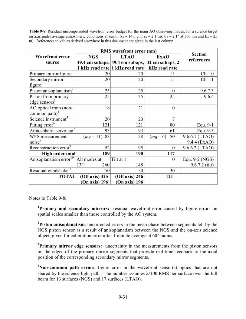
The performance requirements for the different AO modes and design choices motivated by these requirements are collected together in Table 9-7. In addition, Figure 9-12 and Table 9-8 bring together the requirements for wavefront error for the main AO modes. They show how the top level requirement for system wavefront error breaks down into the main component errors of Section 9.2.1. The considerations leading to the value of each component error are developed in the following Sections 9.4 and 9.6. The last column of Table 9-8 gives the specific subsections dealing with each component.

9-29

Table 9-7. AO system performance requirement summary.

AO area Parameter Requirement Driver System Spectral range 0.9 – 25 μm General Maximum FOV

transmitted for AO science instruments

1′ 4′ 8′

NIR Thermal IR GLAO

Corrected field of view to diffraction limit

Not specified Correction over isoplanatic angle with single conjugate

Min. lock hold time 1 hour NIR spectroscopy Flexure 3 mas over 5° elevation change NIR spectroscopy Servo bandwidth -3dB error rejection at 50 Hz High Strehl Emissivity increase ≤2% goal Thermal AO DM Mirror type Single adaptive secondary General Actuator spacing & # 32 cm, 4620 total High Strehl imaging Accuracy of control Individual actuators to 5 nm RMS

Fourier components to 0.26 nm RMS

General ExAO

Servo type Local and global position & speed ” Actuator update rate 2000 Hz ” DM actuator stroke 150 μm Chopping/windshake Full chop angle 4″ Thermal IR 10%-90% chop time 8 ms (goal), 40 ms (requirement) ” LGS Sensor subaperture 0.5 m Beacon configuration Six over 1.2′ to 8′ DL and GLAO SH WFS frame rate 1000 Hz Slope error 0.025″ RMS over a subaperture Total system error 200 nm Tilt sensor band 1-2.5 μm Tilt field 2′ radius Global tilt error 120 nm Sky cover 80% at 30° Galactic lat, 50% at pole Tilt magnitude limit H = 17 NGS WFS

Optical sensor wavefront error

<200 nm RMS LGS slow calibration

IR system wf error 120 nm, 80% Strehl at H for V<8 ExAO GLAO Focal station Direct Gregorian Wavelength range 1 – 2.5 μm Insertion loss <10% Sky cover Anywhere >45° elevation Tip-tilt probes Three, optical STRAP type, 8′ field Segment phasing Not required Image improvement 0.1″ for K seeing <0.4″

9-30

Figure 9-12. Error budgets for the errors listed in Table 9-8 below. The area of each pie reflects the total mean square error (with the total RMS value given numerically below, with corresponding H band Strehl ratio), and the pie sectors show the mean square values of the individual terms. The major error sources are marked and all are color coded to match across the 5 panels. All the charts are for the science target and the center of the laser constellation being on axis. The lower charts show the added error from anisoplanatism when the natural guide star is offset by the given angle. The guides star angular separations are reported at the bottom of the table and their magnitudes at the top.

9-31

Table 9-8. Residual uncompensated wavefront error budget for the main AO observing modes, for a science target on axis under average atmospheric conditions at zenith (r0 = 14.3 cm, τ0 = 2.1 ms, θ0 = 2.1″ at 500 nm and L0 = 25 m). References to values derived elsewhere in this document are given in the last column.

RMS wavefront error (nm) Wavefront error

source NGS

49.4 cm subaps, 1 kHz read rate

LTAO 49.4 cm subaps, 1 kHz read rate

ExAO 32 cm subaps, 2 kHz read rate

Section references

Primary mirror figure1 20 20 15 Ch. 10 Secondary mirror figure1

20 20 15 Ch. 11

Piston anisoplanatism2 25 25 0 9.6.7.3 Piston from primary edge sensors3

25 25 25 9.6.4

AO optical train (non-common path)4

18 21 0

Science instrument5 20 20 7 Fitting error6 121 121 80 Equ. 9-1 Atmospheric servo lag7 93 93 61 Equ. 9-3 WFS measurement noise8

(mV = 11) 83 28 (mH = 6) 50 9.6.6.1 (LTAO) 9.4.4 (ExAO)

Reconstruction error9 52 95 0 9.6.6.2 (LTAO) High order total 189 190 117

Anisoplanatism error10 All modes at 13″: 260

Tilt at 1′: 148

0 Equ. 9-2 (NGS) 9.6.7.2 (tilt)

Residual windshake11 50 50 30 TOTAL (Off axis) 325

(On axis) 196 (Off axis) 246(On axis) 196

121

Notes to Table 9-8:

1Primary and secondary mirrors: residual wavefront error caused by figure errors on spatial scales smaller than those controlled by the AO system.

2Piston anisoplanatism: uncorrected errors in the mean phase between segments left by the NGS piston sensor as a result of anisoplanatism between the NGS and the on-axis science object, given for calibration error after 1 minute average at 60″ radius.

3Primary mirror edge sensors: uncertainty in the measurements from the piston sensors on the edges of the primary mirror segments that provide real-time feedback to the axial position of the corresponding secondary mirror segments.

4Non-common path errors: figure error in the wavefront sensor(s) optics that are not shared by the science light path. The number assumes λ/100 RMS per surface over the full beam for 13 surfaces (NGS) and 17 surfaces (LTAO).

9-32

5Science instrument: another source of non-common path wavefront error contributed by 16 surfaces (NGS and LTAO) and 2 surfaces (ExAO), assuming λ/100 RMS per surface.

6Fitting error: high-order error left over after the best fit is made to the wavefront from the available information. For NGS and LTAO modes, the limit is imposed by the resolution of the Shack-Hartmann sensors. For ExAO, it comes from the actuator spacing on the ASM.

7Servo lag error: residual error introduced by evolution of the wavefront between the time of measurement and correction. The time delay is taken to be 2.5 ms for NGS and LTAO modes, and 1.5 ms for ExAO.

8Measurement noise: photon noise from the guide star introduces an error in the measured wavefront. The NGS and ExAO cases assume operation with a guide star of V magnitude 10 and H magnitude 6 respectively. The LGS case assumes 30 W lasers with DQE of 20%.

9Reconstruction error: for NGS, the main source of reconstruction error lies in not knowing the behavior of the wavefront in the gaps in the pupil. For LTAO, the best tomographic estimation of the wavefront from the six beacons will be in error because information from the LGS is fundamentally incomplete. This is analogous to focal anisoplanatism for a single LGS. It is difficult to quantify without extensive modeling; the number here is drawn from preliminary modeling by Milton & Lloyd-Hart (2003).

10Anisoplanatism: when an off-axis guide star is used, isoplanatic error is introduced between the guide star and science object. For NGS operation, all modes are affected; we give the number for a guide star 13″ off axis. For LTAO, only global tilt is affected because high order modes are derived from the LGS, pointed at the object; we give the number for a guide star 1′ off axis. For ExAO, the target star provides its own wavefront reference and there is no isoplanatic error.

11Windshake: aberration arising from wind buffet, mainly appearing in a resonance of the telescope structure at 8 Hz.

9-33

9.3 Field Development and Tests of Advanced Systems for GMT AO

9.3.1 Introduction

The conceptual design for GMT adaptive optics builds on a program of advanced AO technology development at the University of Arizona, in collaboration with l’Osservatorio di Arcetri, funded by the AFOSR, the NSF, and NASA, for the specific issues of extremely large telescopes. In addition, Carnegie Observatories have been making experiments toward ground layer correction at Las Campanas. Four areas are of particular relevance to GMT and are discussed below.

9.3.2 Adaptive Secondary Mirrors

The MMT adaptive secondary mirror, Figure 9-13, is the first of its kind and is now in routine use for scientific observation. It has already demonstrated the unique power of secondary correction for the thermal IR (Liu et al. 2005). The accuracy of wavefront correction achieved with the single element with 336 actuators is similar to conventional systems with correction in an optical relay with five or more additional surfaces including separate mirrors for tip-tilt and higher order correction.

Figure 9-13. MMT deformable Cassegrain secondary, mounted in the telescope at sunset.

The location and large stroke of the adaptive secondary allows for all the correction at the single surface, including tip-tilt. This removes the need for the additional optical train, and the Cassegrain image passes directly into the instrument dewar, whose entrance window reflects optical light to the wavefront sensors. The secondary is currently used with a Shack-Hartmann sensor in a system that corrects 56 modes. The typical Strehl is 20% at H and 98% at N-band. The H band Strehl is currently limited by vibration of the telescope mount. Accelerometers are

9-34

being installed so the motion can be sensed and corrected, to reach the 30% Strehl shown by current fast-framing data after residual image motion has been corrected. The RMS wavefront error of 290 nm RMS after vibration correction is similar to the 260 nm RMS for the Keck NGS AO system (van Dam et al. 2004). Table 9-9 compares the two systems.

The deformable secondary mirror technology was developed in conjunction with Arcetri Observatory in Italy, with the two deformable secondaries now being built for the LBT as a major goal. At 0.9 m diameter and with 672 actuators each, the LBT secondaries will serve as near full-size prototypes for the GMT secondary segments.

Table 9-9. Comparison of Keck and MMT AO performance.

MMT Keck Shack-Hartmann subaperture size

0.54 m 0.56 m

WFS frame rate 550 Hz 670 Hz Normalized number of modes corrected

1.9/m2 3.1/m2

RMS wavefront error (bright reference star)

290 (tip-tilt removed) 260

9.3.3 Wavefront Sensing with Multiple Laser Guide Stars

Until recently, no telescope had attempted wavefront sensing using more than one LGS. Within the last two years, the first tomographic wavefront sensor using multiple laser beacons has been built and tested at the MMT, by the University of Arizona. This prototype of the tomographic wavefront sensing system to be used at the GMT uses Rayleigh beacons range gated at 25 km altitude. Because of the smaller aperture, the 6.5 m is a good scale model for tomography with the 25 m GMT using sodium beacons at 90 km altitude. The range gate used at the MMT is 9 km, from 20 to 29 km. This range gate results in large spot elongation, about 8″ for the edge subapertures. This is corrected by focusing with a mirror oscillating at the 5 kHz pulsed laser frequency, the first field test of any system to correct spot elongation.

The constellation diameter is set to 2′, representing a compromise between the ideals for LTAO and GLAO. The five beacons are derived from two 15 W doubled YAG lasers at 532 nm, pulsed at 5 kHz. The unique Shack-Hartmann sensor places all five beacons on a single detector, with electronic shuttering to implement the beacon range gate (Figure 9-14). For each laser beacon there are 60 subapertures in a hexapolar pattern, with a subaperture dimension of 0.7 m. A separate WFS with 0.5 m subapertures analyzes light from a natural star within the LGS field.

The data comprise simultaneous measurements of wavefronts sensed by the beacons and a series of natural stars. We have found that the average beacon wavefront gives a good measurement of ground layer aberration, and that tomographic reconstruction of the five beacon wavefronts allows estimation of the stellar wavefront in any chosen direction within the field enclosed by the beacons (Lloyd-Hart et al. 2005).

9-35

Figure 9-14. Single frame from the 5-beacon Shack-Hartmann sensor. All five patterns are imaged onto a single electronically gated CCD with 16 output channels with up to 1 kHz frame rate.

Wavefront data have been recorded during two telescope runs in September 2004 and June 2005. During the earlier run, the seeing was 1.0″ in V, worse than median for the site, but was 0.5″ during the June run. The results of ground-layer correction, in which the instantaneous average of the five LGS wavefronts is used to correct the simultaneous wavefront from a natural star, are shown in Figure 9-15 as a function of the field angle between the star and the geometric center of the LGS constellation.

Figure 9-15. Results of ground layer estimation from the MMT laser guide stars. The RMS residual after correction of a stellar wavefront by the average of the five laser wavefronts is shown as a function of field angle for data recorded during two separate telescope runs. The corresponding uncorrected values, constant with field angle, are shown as dashed lines for September 2004 (upper) and June 2005 (lower).

These data provide the first experimental evidence of the gains to be expected from GLAO. In both cases, correction extends beyond the radius of the LGS constellation. Note too that though the fractional improvement in the residual wavefront aberration was greater in the September data, the absolute improvement was better in the June data, when the natural seeing was twice as good. This supports the view emerging from numerical simulations that GLAO will be of particular value when the seeing is poor.

9-36

From the residual wavefront errors, an estimate of the corrected PSF can be calculated. Figure 9-16 shows examples calculated for J band from 60 s of data. Table 9-10 below shows the widths and relative peak intensities for PSFs calculated from the June results. At J band, there is modest improvement in image width with ground-layer correction, and a factor of two improvement in peak intensity. At K band, the correction is sufficient to reach within a factor of two of the diffraction limit. Also shown in the table is the effect of tomographic correction, where the goal is not to separate the ground layer contribution common across the field, but to reconstruct the integrated wavefront error along a single line of sight. In this case, the K band is corrected almost to the diffraction limit, with a 14-fold increase in peak intensity. The relatively low order reconstruction attempted to correct only the first 45 Zernike modes, which was insufficient to achieve the diffraction limit in J, but the improvement in resolution and peak brightness are both substantial.

Figure 9-16. Synthetic J-band PSFs calculated from the corrected and uncorrected natural star wavefronts.

Table 9-10. Performance of open loop GLAO and tomography from the MMT, where the diffraction limit is 0.04″ in J band and 0.07″ in K band.

Wave band

Uncorrected Ground-layer correction

Tomographic correction

FWHM (arcsec) 0.44 0.38 0.10 J Relative peak 0.26 0.50 1.00 FWHM (arcsec) 0.40 0.12 0.09 K Relative peak 0.07 0.47 1.00

Reconstructors for full tomographic recovery of the on-axis wavefront have now been computed from portions of the simultaneous natural and laser star wavefronts, by filtered singular value decomposition. Estimates of the stellar wavefronts are calculated from the laser wavefronts from other portions of the data, using the reconstructors. An example comparing the measured and estimated amplitudes of the focus term for a 10 s data sequence is shown in Figure 9-17 where we show the comparison with both the GLAO and LTAO estimates. Figure 9-18 illustrates the RMS wavefront error summed over all 54 sensed modes. Tip-tilt is deliberately excluded because it contains the majority of the wavefront error, yet is easiest to sense and correct. It therefore gives a somewhat misleading sense of the overall degree of correction.

0.5 arcsec

Uncorrected Ground layer corrected Corrected by tomography

1.25 μm

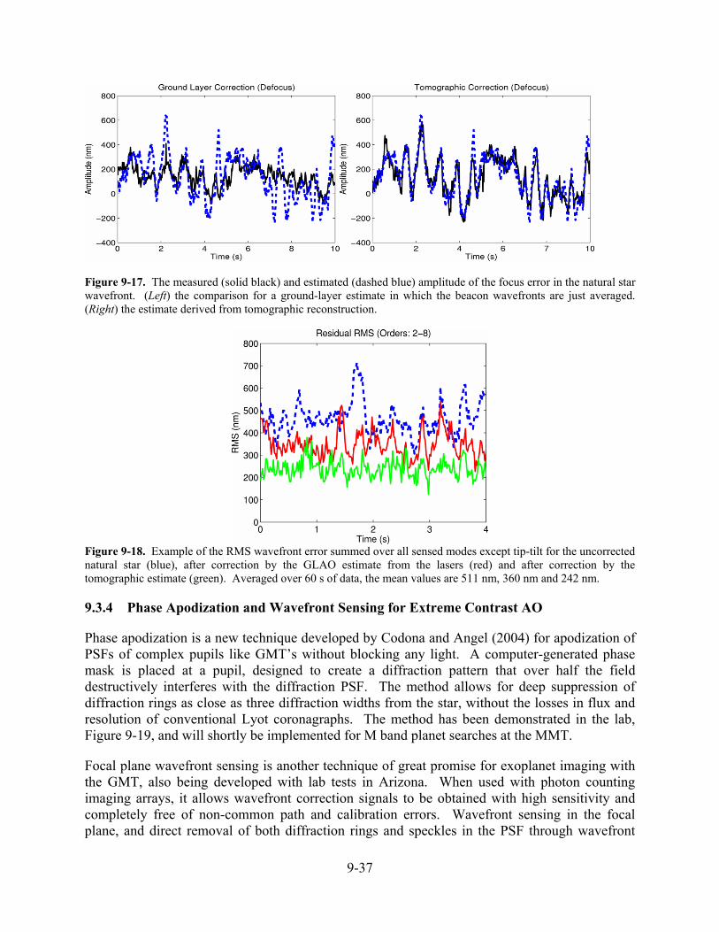
9-37

Figure 9-17. The measured (solid black) and estimated (dashed blue) amplitude of the focus error in the natural star wavefront. (Left) the comparison for a ground-layer estimate in which the beacon wavefronts are just averaged. (Right) the estimate derived from tomographic reconstruction.

Figure 9-18. Example of the RMS wavefront error summed over all sensed modes except tip-tilt for the uncorrected natural star (blue), after correction by the GLAO estimate from the lasers (red) and after correction by the tomographic estimate (green). Averaged over 60 s of data, the mean values are 511 nm, 360 nm and 242 nm.

9.3.4 Phase Apodization and Wavefront Sensing for Extreme Contrast AO

Phase apodization is a new technique developed by Codona and Angel (2004) for apodization of PSFs of complex pupils like GMT’s without blocking any light. A computer-generated phase mask is placed at a pupil, designed to create a diffraction pattern that over half the field destructively interferes with the diffraction PSF. The method allows for deep suppression of diffraction rings as close as three diffraction widths from the star, without the losses in flux and resolution of conventional Lyot coronagraphs. The method has been demonstrated in the lab, Figure 9-19, and will shortly be implemented for M band planet searches at the MMT.

Focal plane wavefront sensing is another technique of great promise for exoplanet imaging with the GMT, also being developed with lab tests in Arizona. When used with photon counting imaging arrays, it allows wavefront correction signals to be obtained with high sensitivity and completely free of non-common path and calibration errors. Wavefront sensing in the focal plane, and direct removal of both diffraction rings and speckles in the PSF through wavefront

9-38

phase control, have been shown in closed loop in the lab (Codona et al. 2006). These techniques are the basis of direct planet detection planned with the GMT.

Figure 9-19. Lab demonstration of phase apodization of the Airy pattern, with strong suppression at 2 λ/D.

9.3.5 Coherent Phasing of Wavefront with Discrete Segments

In experiments with the old six mirror MMT, the Arizona team demonstrated diffraction-limited performance of the telescope with the segments cophased in real time, Figure 9-20, using two different focal plane natural star wavefront sensing techniques (Angel et al. 1990, Lloyd-Hart et al. 1992, Lloyd-Hart et al. 1993). One of these relied on phase diversity to break the symmetry in the focal plane. Phase steps between pairs of segments with the same baseline vector produce identical results in an image at the focal plane, but by examining a pair of simultaneous images with a known focal shift between them, it is possible to solve unambiguously for the wavefront error. The only parameters sought are the piston errors between distinct pieces of wavefront that define localized regions in Fourier space. It is therefore possible to solve directly for these errors from the transform of the image rather than relying on a full-blown iterative phase diversity algorithm. The methods pioneered at the MMT will serve as the basis for the stellar phase calibration sensors planned for the GMT segments.

Figure 9-20. Coherent phasing at the old MMT. With five of the six segments open, the beams were cophased at 40 Hz by examining the Fourier transform of the coherent image at 2.2 μm. A similar technique will be used to cophase the GMT with natural starlight for diffraction limited AO modes.

9-39

9.4 Wavefront Sensing Strategy and Hardware

The GMT AO system will use a range of sensors to determine the wavefront correction signals. The measurements will be of natural stars in the optical and infrared, and of laser beacons at 589 nm. The focal plane data will be augmented by data from mechanical sensors of the relative position of primary segments and from accelerometers on the secondary support frame. This section sets out the strategy for wavefront sensing, identifying the required sensors, which we then describe. The control system that links these sensors and the projected performance of the overall system is given in Section 9.6.

9.4.1 Overall Strategy for Wavefront Measurement

The wavefront errors to be controlled can be divided into high order errors from atmospheric turbulence, global tilt errors from the atmosphere, vibration, and wind buffet, and piston errors between the segments from all sources. All these errors must be controlled to high accuracy in all AO modes, with the exception of inter-segment piston errors in the case of GLAO. The most general case is control to the diffraction limit using LTAO, which uses most of the hardware elements of the AO system. The overall picture for controlling the wavefront in this mode of operation is shown in Figure 9-21.

9.4.1.1 LTAO Sensing of High Order Errors

High-order errors over the individual 8.4 m segments are to be sensed from the laser beacon constellation. To do this, laser light (yellow in Figure 9-21) is passed by the middle dichroic in Figure 9-4 and reflected by the low dichroic to the Shack-Hartmann sensors, one per beacon. Although global tilt cannot be recovered from the LGS measurements, all other modes across the pupil are reconstructed from the slopes measured across the full aperture. The 24.4 m pupil wavefront is recovered in the reconstruction, but the gaps between segments cause an additional error component of ~50 nm in normal seeing, as shown in Section 9.6.7.3.

As has been found at the Keck II telescope, drift of the LGS sensors and unknown variations in the height of the sodium layer mean that periodic calibration against a slow NGS sensor is essential. Optical light from a field star will be used for this (blue in Figure 9-21), transmitted to a separate CCD Shack-Hartmann sensor that divides the pupil with the same subaperture configuration as the six LGS sensors. Information from this sensor will be used to update a table of centroid offsets in the LGS real-time subaperture slope calculator, and the axial positions of the LGS sensors themselves to accommodate changes in range of the sodium layer. Depending on the brightness of the NGS and the time needed to average out anisoplanatism, updates from it will be computed on a timescale of tens of seconds.

9.4.1.2 Measurement of Global Tilt

Global tilt sensing for the GMT will be of the IR image of the same field star used for LGS calibration, reflected to the IR wavefront sensor unit. The IR is chosen because in the visible (λ<1 μm) the wavefront remains largely incoherent, even after AO correction. Thus from a visible sensor global tilt can only be recovered to an accuracy limited by the seeing width. On the other hand, a measurement to high accuracy can be made from a sensor that sees the image of

9-40

a natural guide star sharpened by the LTAO, as for the case in the near IR of a star close to the axis of LTAO correction. At 60” separation though, high-order anisoplanatism will reduce the deformable-secondary correction to the seeing limit, even in the near IR. High quality imaging will be restored from the multi-laser sensor by correcting the stellar wavefront separately using the technique of multi-object adaptive optics (MOAO). The tomographic wavefront solution derived from the LGS will be integrated along the line of sight to the tilt reference star, just as it is for the line of sight to the science object. After the solution for the science object is applied to the adaptive secondary, a small DM in the tilt sensor path will be adjusted to give the additional differential correction required for the guide star.

Figure 9-21. Overview of the wavefront control paths for GMT. The thick black line at 45° represents the middle dichroic of Figure 9-4, transmitting the optical and reflecting the near infrared.

9-41

A 1024 actuator MEMS DM in the path to the tilt sensor will be used to correct for the angular anisoplanatism, correcting the H-band image of the star to Strehl ratio of 50% under median conditions. No differential tilt correction will be applied, since that is rather the quantity to be sensed. The required stroke is then just 2 μm, already within the capabilities of MEMS devices. The infrared advantage for tilt sensing increases for very large telescopes since not only does the image become sharper, but the flux in the image increases. Furthermore, the increase in image sharpness with larger aperture reduces the noise from underlying sky background because smaller sensor pixels may be used. Figure 9-22 illustrates the pixel scale to be used in the tilt sensor and the NGS piston sensor discussed in the next section. Thus for a guide star at H = 17 at 50% Strehl ratio, the diffraction core surface brightness is ~9th mag/arcsec, still 40× brighter than sky background of H = 13 per square arcsec. Location of the tilt sensors - the near IR light reflects off the middle dichroic (Figure 9-4 and Figure 9-21) and into the wavefront sensor unit that precedes the Offner relay to the science instruments. Here it will be picked up by one of three separate tilt sensors fed by probe mirrors that each patrol 1/3 of the central 4′ field. The probes are small to cause least disruption to the field that passes by to be reimaged into the science instruments.

Figure 9-22. The diffraction limited PSF in H band shown in a linear z-scale with a grid overlaid illustrating the 14 mas pixel size to be used in the near IR global tilt sensor. The four central pixels for tilt sensing would be implemented by four separate fiber-fed TES detectors. The same pixel scale will be used in an array as the NGS piston sensor, Section 9.4.1.3. Use of such small pixels enormously reduces sky background contamination compared to a seeing limited sensor.

Wind-induced vibrations of the telescope also contribute to image motion. Experience at the MMT, and at Keck and Gemini, has shown that even at present large telescopes the motion can be difficult to control just with the AO optical loop. The amplitude of such resonances on the GMT will be larger, though finite element modeling shows they are expected to have most power in modes clustered around a relatively benign 8 Hz. To supplement the IR NGS tilt measurements, accelerometers mounted on the secondary mirror structure will provide feedback to the real-time reconstructor on vibrations of the mirror. Four triaxial accelerometers have been mounted on the MMT’s secondary to deal with 20 Hz vibrations there, and we will shortly understand how such data should be combined with the optical tilts in the real-time loop.

0.08″

9-42

9.4.1.3 Inter-Segment Piston Control

For all segmented mirrors the absolute wavefront steps across the gaps between the segments must be measured and periodically calibrated absolutely by interferometry from a natural star. For the GMT the 30 cm gaps require that the interfering baseline be at least this long. Because the full pupil has only seven segments, the NGS piston measurement can be recovered at high speed and high accuracy for even quite faint guide stars on-axis. Nevertheless, field anisoplanatism will limit the value of such sensing in the general LTAO case.

It is possible that the MOAO solution to the anisoplanatic problem described for global tilt sensing may also work for the piston sensor, but the requirement is an order of magnitude more challenging. For tilt, one need only correct the wavefront well enough to give the star image reasonable Strehl ratio, but for the piston a recovery of the mean phase across the segment gaps to a few tens of nm is needed. Instead we adopt as baseline an approach similar to the high-order correction: fast measurement sensors supplemented by periodic calibration.

For fast piston sensing, the primary segment edge sensors will be used to correct the wavefront reconstructed from the global Shack-Hartmann data. This reconstruction recovers piston differences arising from the continuous atmospheric wavefront aberration, but insensitive to discontinuities in piston induced by wind buffeting and vibration of the segments. These motions will be determined by edge sensors that will bridge the 30 cm gaps optically to recover with 20 nm accuracy. Fast correction of the total piston errors will be made with the secondary mirror, while the error build up from mechanical motions will be offloaded to the primary mirror actuators on time scales of several minutes.

Periodic absolute calibration will be made with a small fraction of the near IR NGS starlight forming two defocused images on a separate small detector array built into each tilt sensor. These images will be read out about once a minute, and a phase-diversity algorithm will recover the six long-term average relative piston errors from the image pair.

9.4.1.4 Strategy in Other AO Modes

For GLAO the lasers will also be used, in a constellation now spread to 8′ diameter. In this case, the strategy and equipment for wavefront sensing and correction will be the same as described above for LTAO with the exception of piston sensing. Since the diffraction limit of the individual apertures is sharper than the combined GLAO image, piston errors can be ignored. The general shape of the primary mirror will still be kept under control by the active optics system, with periodic reference to the segment edge sensors.

The classic NGS AO mode will be available, without lasers, when an adequately bright natural star is available for the science program. In the case of exoplanet searches when the primary star is bright it will always provide the wavefront reference. Two NGS wavefront sensors are provided. The visible Shack-Hartmann sensor normally deployed to calibrate the LGS sensors may be used also at high speed, offering a conventional NGS capability with 0.49 m subapertures, and for magnitudes V<11 is expected to outperform LTAO. Also available will be a near IR pyramid sensor (PRWFS) in front of the Offner relay and in the same area as the near IR tilt and piston sensors. With scalable subaperture size down to 0.32 m, it will be sensitive

9-43

over a range of guide star brightness. Anticipating the availability of low noise IR array detectors, the PRWFS is likely to be the preferred NGS sensor except when near IR science requirements preclude its use, because of its inherently higher accuracy determination of low-order modes than the Shack-Hartmann sensor.

9.4.2 The Optical and Infrared Wavefront Sensors

At present the natural star wavefront sensors in almost all AO systems use silicon detectors with high quantum efficiency for wavelengths <0.9 μm. This reflects current technology, in which optical detectors, both arrays (CCDs) and point detectors (avalanche diodes) are faster and quieter than their near infrared counterparts. But the flux of a typical K5 field star at wavelengths longer than 0.9 μm is more than twice that below 0.9 μm, as shown in Figure 9-23, and as we have seen, much greater accuracy in measurements of low order aberrations will be possible with sensors in the near IR. Thus it will be highly desirable for the GMT to make additional natural star wavefront measurements in the near infrared. On the time scale of the GMT, the potential for infrared sensors with comparable sensitivity as today’s optical sensors looks good, as we discuss in section 9.4.3 below.

Figure 9-23 Total photon flux incident on the GMT from a typical K5 faint field star (H = 17, V = 19). Photons below 0.9 μm (dashed line) can be efficiently detected with a CCD.

Anticipating the use of IR detectors, the GMT AO architecture is arranged with dichroic separation at 1 μm to deliver the same wide field to two separate stations, both equipped with wavefront sensors. In many cases, the brightest and closest field star will be sensed at both stations simultaneously, so that all its light can be used to best advantage. In the following sections we describe the suite of optical and infrared sensors summarized in Table 9-11.

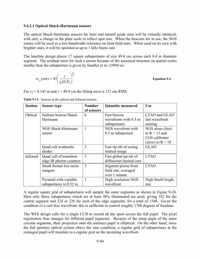
9-44

9.4.2.1 Optical Shack-Hartmann sensors

The optical Shack-Hartmann sensors for laser and natural guide stars will be virtually identical, with only a change in the plate scale to reflect spot size. When the beacons are in use, the NGS sensor will be used as a low-bandwidth reference on faint field stars. When used on its own with brighter stars, it will be operated at up to 1 kHz frame rate.

The baseline design places 17 square subapertures of size 49.4 cm across each 8.4 m diameter segment. The residual error for such a sensor because of the unsensed structure on spatial scales smaller than the subaperture is given by Sandler et al. (1994) as:

56

0

( ) 43(0.5)fitsnm

rσ

⎛ ⎞= ⎜ ⎟

⎝ ⎠ Equation 9-4

For r0 = 0.143 m and s = 49.4 cm the fitting error is 121 nm RMS.

Table 9-11. Sensors at the optical and infrared stations.

Station Sensor type Number of sensors

Quantity measured Use

Sodium beacon Shack-Hartmann

6 Fast beacon wavefronts with 0.5 m subapertures

LTAO and GLAO fast wavefront sensing

NGS Shack-Hartmann sensor

1 NGS wavefront with 0.5 m subaperture

NGS alone (fast) to R = 13 and LGS calibrator (slow) to R = 18

Optical

Quad cell avalanche diodes

3 Fast tip-tilt of seeing limited image

GLAO

Quad cell of transition edge IR photon counters

3 Fast global tip-tilt of diffraction limited core

LTAO

Small format low noise imagers

3 Segment piston from field star, averaged over 1 minute

LTAO

Infrared

Pyramid with variable subapertures to 0.32 m

1 High resolution NGS wavefront

High Strehl bright star

A regular square grid of subapertures will sample the outer segments as shown in Figure 9-24. Here only those subapertures which are at least 50% illuminated are used, giving 192 for the central segment and 224 or 226 for each of the edge segments, for a total of 1540. Given the condition of a curl-free wavefront, this is sufficient to control roughly 1700 degrees of freedom.

The WFS design calls for a single CCD to record all the spots across the full pupil. The pixel registration thus changes for different pupil segments. Because of the steep angle of the outer circular segments, their projection onto the entrance pupil is elliptical. On the other hand, since the full aperture optical system obeys the sine condition, a regular grid of subapertures at the reimaged pupil will translate to a regular grid on the incoming wavefront.

9-45

A 256×256 pixel CCD will be used. For the NGS, the pixels will subtend 0.5″ and the detector will be configured with a 4×4 pixel image of each spot with a one-pixel guard band. For highest sensitivity the lenslets will be aligned as in the MMT sensor so that for a flat wavefront the spots are centered on the intersection of 4 pixels. If the CCD has 15 μm pixels a collimated pupil image 3.75 mm across would be formed on lenslets 75 μm square at f/15. The CCDs will be read out at full resolution at 1 kHz frame rate. The total pixel rate is thus 65 Mpix/s, a realistic extrapolation from current practice. For example, the MMT LGS program’s Shack-Hartmann sensor uses a 128×128 CCID18 from MIT’s Lincoln Lab, read at 14.7 MHz with 16 amplifiers running at near 1 MHz rate with 7 e- RMS noise. For the GMT, in order to reach a read noise of 3 e-, each CCD will need 256 channels, read at 256 kpixel/s per amplifier. CCDs with 64 amplifiers are already made, so the extension to 256 is realistic. A readout architecture would be chosen in which all 5×5 pixels in a sub-array go to the same amplifier. This will be done with serial registers passing between columns of pixels, so amplifiers could service five rows of 50 columns. This type of architecture is being developed for the LSST CCDs (Geary et al. 2005).

Figure 9-24. The arrangement of 1540 subapertures for the optical Shack-Hartmann wavefront sensors. The 50×50 spot array will be imaged onto a 256×256 pixel detector. The same CCD and optical format would be used for the laser beacons sensors. However, since in this case because the spots are radially streaked, the lenslet focal ratio will be decreased so the pixels subtend 1.0″ for a 4″ square field. If needed, further angular separation of the streaked spots can be achieved by using anamorphic lenses that include a cylindrical component in the radial direction. Recovery of centroids will be done by cross correlating each measured 4×4 spot image (ignoring the guard band pixels) with fixed template images matched to the expected shape of the spot at each subaperture. Unlike the conventional center-of-mass calculation, which weights most heavily those pixels at the edge of the subaperture that contain the least light and therefore have the lowest signal-to-noise ratio, this technique places most emphasis on the illuminated pixels (Poyneer & Véran 2005).

9-46

Given that the seeing limited spot images of both NGS and LGS will have broad wings, a field stop matched to the size of a subaperture will be required in front of each WFS. In this way, beacon light will be prevented from bleeding from one subaperture to its neighbors, incorrectly biasing the measured slope signals. Table 9-12 summarizes the characteristics of the optical Shack-Hartmann sensors.

Table 9-12. Shack-Hartmann parameters.

LGS and NGS wavefront sensors Shack-Hartmann, 7 in all Subaperture size and number 0.49 m square, 1540 spots per sensor Frame rate 1 kHz Detector CCD, 256 pixel square, Readout 256 channels @ 250 kHz/ch. @ 3e- RMS read noise Correlation field per subaperture 4″ (LGS) 2″ (NGS) Pixel size 1″ (LGS), 0.5″ (NGS) (5×5 per subaperture)

9.4.2.2 Optical Tip-Tilt Sensors

The optical tip-tilt sensors are quad cells with four photon counting avalanche silicon diodes. These have high quantum efficiency from 0.4–0.9 μm wavelength, and are widely used in today’s 8 m class AO systems. On GMT they will be used primarily for GLAO. Three sensors will be used, fed by pick-off mirrors in the natural star focal plane ahead of the beacon Shack-Hartmann sensors.

9.4.3 Infrared Sensors

9.4.3.1 Detectors

IR array detectors exist already that are adequate for the fast tip-tilt and slow piston calibration measurements to be made at the GMT. The best in use today is the HAWAII 2 array, read out through a single channel at a 1 MHz pixel rate with 10 e- RMS noise, two to three times the read noise of fast CCDs. For fast full aperture wavefront sensing, new arrays with multiple outputs are being designed specifically for AO and interferometry. For example, ESO and Caltech are developing with Rockwell a HgCdTe 128×128 pixel device, “Calico”, with eight parallel outputs, a frame rate of up to 2.7 kHz and a projected noise of 7 e- RMS at 800 frames/s (Finger et al. 2004). Since the pixel rate per channel and noise represent only a modest advance (50% improvement) compared to HAWAII 2, it is reasonable to plan for devices at least this powerful on the time scale of the GMT.

For single photon counting in the near infrared, point detectors fed by single mode fibers exist already. These are transition edge sensor (TES) detectors, the equivalent for λ>1 μm of silicon avalanche detectors. They detect single photons when they are absorbed by a thin island of tungsten just cold enough to be superconducting (100 mK). The deposited energy is detected as a momentary increase in resistance. These detectors are being built at NIST for quantum computing and quantum cryptography, and have now reached the high performance levels needed for astronomy (Rosenberg et al. 2005). The current version optimized for detection at 1.55 μm has a level of performance that would be already suitable for a near infrared quadcell

9-47

for the GMT (Figure 9-25). The single element detector has a quantum efficiency of 88%. Dark current at the operating temperature of ~100 mK is negligible. The dead time between pulses is <10 μs, allowing for count rates up to 10,000/sec with little saturation. The AR coating in the NIST detector was tailored for 1.55 μm, but has high efficiency across the H band. Other detectors could be tailored for the K band detector with absorption from 2 to 2.4 μm.

Figure 9-25. Transition edge sensor photon counting detector performance at 1.55 μm wavelength. The quantum efficiency is 88% over the H band. The plot is a histogram of the signal level measured at the known time of arrival of a weak pulse averaging 3 photons.

It seems that on the timescale of the GMT high sensitivity imaging arrays of TES photon counters could be developed. Already TES detectors of 20% QE have been built in arrays as large as 8×8 pixels, and have been used in astronomy (Romani et al. 2001). The technology for making such arrays is similar to that developed for SCUBA 2 at the JCMT, which also uses transition edge superconductor bolometers, again developed by NIST but in this case optimized for detection in the submillimeter with a molybdenum/copper superconductor at 120 mK. SCUBA-2 will use several 40×32 element arrays (Audley et al. 2004).

9.4.3.2 Tip-Tilt Sensor and Limiting Magnitude

The advantage of sensing tip-tilt in the near IR may be quantified as follows. The image width in the optical seeing limit is λ/r0, i.e. ~0.6″. For the H band diffraction limit, where Deff = 24.4 m for the GMT, the width is λ/Deff or 0.014″. The photon fluxes incident on the telescope for the H = 17 guide star of Figure 9-23 will be 180/ms for a CCD detector sensing below 0.9 μm and ~80/ms for the H band diffraction core, assuming 50% Strehl. The photon noise limited error in tip-tilt will be in the ratio 0.6/0.014 × √(80/180) = 28. Since the error is proportional to 1/√N, where N is the photon flux, the same accuracy in the optical as in the H band would require a star 800× or 7 magnitudes, brighter. Even with this advantage, the scarcity of bright stars within the isoplanatic angle for tilt at high Galactic latitude puts a premium on using the highest possible sensitivity for the tilt sensor detector (see Section 9.6).

9-48

The GMT will use an H band quad cell using 4 TES detectors with single mode fiber feeds. Pupil shaping optics will be used to couple the field segments to the fibers with little loss. The tilt sensitivity at H = 17 is calculated here, since we will find that stars at this magnitude must be used to get all-sky cover. Assuming 40% effective quantum efficiency in the H band for the telescope, optics and detector, the H band photon detection rate will be N ~ 32/ms for the diffraction core. These counts will be distributed as approximately 8 in each quadrant of the quad cell sensor. TES detectors have no read noise, and with negligible H band flux from sky background as discussed above, the slope error for the quad sensor (Sandler et al. 1994) is 0.7 λ/D√N = 1.6 mas/√t(ms).

9.4.3.3 Segment Piston Sensor

The NGS pyramid sensor has the potential to provide piston information (Esposito et al. 2003), but we plan to use dedicated high sensitivity sensors aimed specifically at piston sensing of faint field stars. The data they provide will be used with both the NGS and LGS Shack-Hartmann sensors in the diffraction-limited imaging modes. The arrays will be incorporated with the tip-tilt sensors used for fast image motion control, and will share a small fraction of the infrared light from the same star.

Chanan and Pinto (2004) have tested a technique for phasing the Keck, where the telescope was defocused to the point that the 36 segment boundaries could be distinguished in the defocused images. For the Keck 36 segment system an iterative procedure, starting with images taken in narrow bandwidth L and ending with broadband K, was projected to give 20 nm RMS wavefront accuracy for a bright star. In our case we have only six piston differences to measure, a less challenging problem. Two approaches to the sensor are being considered. Our baseline design derives the piston information by phase diversity from two images formed simultaneously, with small known defocus terms of equal magnitude and opposite sign introduced into them. An example of measuring a piston error with defocus for the GMT is given in Figure 9-26. Here the defocus is ¼ wave RMS in the K band, and the effect of a 400 nm displacement appears clearly in the defocused images. Standard phase diversity methods would be used to recover the piston values.

Figure 9-26. GMT PSFs in the K band either side of focus (A and B). The segments are in phase except for the outer segment at 6 o’clock which had 400 nm piston error. The difference image is on the right. Such phase diverse images will be used to recover piston errors between segments averaged over ~1 minute.

A second approach we will investigate would extend the method of Lloyd-Hart et al. described in Section 9.3.5. The functioning of this sensor is illustrated in Figure 9-27. The GMT pupil is split into three different configurations, and an in-focus infrared star image is formed from each. This is done with little loss of light with dielectric beamsplitters in the pupil. The first redirects

9-49

half the light from the ring of six outer segments to form the bottom diffraction limited image in the second column of Figure 9-27. The remaining light is split again at the pupil to form the two upper pupils and images. The fifth and sixth columns show the MTFs of the three images for the cases of piston error in the 9 o’clock segment (PSF in the third column) and in the center segment (PSF in the fourth column).

Both methods are viable and a selection will be made pending further analysis. Their sensitivity to detector and photon noise and to anisoplanatic effects will be investigated. For calibration once per minute, a Hawaii 2 array would be completely adequate. For real time piston measurements of a star on or near axis, this approach could be adapted to encode the piston information in as few as 18 pixels, which could be sensed by 18 TES sensors with zero read noise placed on the six peaks in the first Airy ring in the three images. About half of the signal from the star would go into the detectors. The flux of 400 photons in 10 ms from a star of H = 17 would allow piston measurements to be made in this integration time.

Figure 9-27. Tip-tilt-piston sensor. The GMT pupil is split in 3 parts (column 1), and a stellar PSF formed from each (columns 2, 3, 4 for no error and ¼ wave in an outer and the central segment respectively). The corresponding MTFs for the aberrated cases (columns 5 and 6) encode the segment piston errors. The field of view required for the detector array is out to the first Airy minimum of the 8.4 m subapertures, i.e. 7.5 λ/D for the full aperture.

9.4.4 High Resolution NGS Sensor

To reach the goal of 120 nm RMS closed loop wavefront error for high fidelity correction a very fast low noise array detector is needed. An optical sensor with the required speed and resolution will likely be available, and could be used in a Shack-Hartmann sensor scaled up from the Starfire Optical Range (SOR) design, which has achieved 112 nm RMS on a V = 5.7 star (Fugate et al. 1999). Such a design would be a fallback position for the GMT. But an IR sensor with the necessary speed and resolution is preferable, and we take this as our baseline.

9-50

To take full advantage of the IR, the sensor must exploit the coherence of the corrected wavefront, as do the IR tip-tilt and piston sensors. Since the advantage is present only when the wavefront has been corrected to some coherence already, the optical Shack-Hartmann sensor looking at the program star would be used to bootstrap the correction to the level of 200 nm RMS residual error. Two wavefront sensors will be explored that would use the IR from the same star to correct further to the 120 nm goal: the stationary pyramid sensor (Ragazzoni & Farinato 1999) and the Mach-Zehnder interferometric wavefront sensor (Angel 1994, 2003).

Pyramid sensors operate by dividing the starlight into four beams by focusing the image of the star at the tip of a four-sided pyramid. Four images of the pupil, one for each beam, are then formed and measured simultaneously. Pyramid sensors have been successfully demonstrated in the lab, including in closed loop AO systems (Esposito et al. 2000) and in preliminary telescope tests at the TNG (Ghedina et al. 2003). Pyramid sensors with CCD detectors are being built for the facility adaptive optics system for the Large Binocular Telescope, by a group at Arcetri Observatory. The LBT AO system is currently being tested with delivery to the telescope planned for 2006.

The alternative is a Mach-Zehnder interferometer used as a variant of the self-referenced Zernike interferometer. In this design, the light in the diffraction core is separated by a small optical element in the focal plane to form a reference beam which is then recombined to interfere with two or four pupil images. These are recorded simultaneously, just as for the pyramid sensor. A closed loop AO system based on a Mach-Zehnder sensor has been demonstrated in the lab (Codona et al. 2006) and was used to produce the diffraction suppression PSF in Figure 9-19.

Both pyramid and interferometric sensors require accurate guiding of the IR diffraction core, and both need similar IR sensors. If a separate array is used for each of four pupil images, each one must have 80×80 pixels to record the full pupil image with 32 cm resolution. A frame rate of 2 kHz would be preferred, i.e. 13 Mpixel/s for each array.

Let us calculate the limiting magnitude supposing that a detector with 7e- RMS read noise is available for use at the GMT, and that it is operated with read and photon noise balanced, i.e. at a photon flux that yields 50 photoelectrons per pixel per read per pupil image. The signal/noise ratio would then be 5 per pixel. For the interferometer, and likely the pyramid sensor also, this will result in an RMS wavefront error of ~λ/(2π(S/N)) = 50 nm for H band sensing. Assuming 30% DQE and 2 kHz read rate, the H band magnitude corresponding to the above photoelectron signal is H = 6.3. This is already a very useful limit for high contrast imaging of nearby stars.

This projected limit is in reasonable agreement with extrapolation from VLT experience with their Shack-Hartmann IR sensor. When used with 1.4 m2 subapertures at 160 Hz frame rate, it ceases to be read noise limited for K<11. If we scale for subapertures of 0.1 m2 at 2 kHz we require a flux 175× higher, or an increase in magnitude from 11 to 5.6.

The final choice for the GMT for the high resolution IR sensor will depend on experience developed at the LBT, and the evolution to IR sensor arrays that can exploit fully the potential gain of a high resolution IR system. An example of what might be achieved in pushing to fainter magnitudes if lower noise detectors are realized is shown in Figure 9-28. The sensitivity is modeled for an IR Shack-Hartmann sensor, using the entire photon flux from 0.9 – 2.4 μm and

9-51

assuming an infrared sensor with a read noise of 3 e- RMS. For Strehl ratio of 0.8 in K, corresponding to 165 nm RMS wavefront error, the limiting V magnitude equivalent is 9.6, corresponding to H = 7 for the assumed K5 star. The pyramid sensor is projected to be about 1 magnitude more sensitive. An increase in integration time to 5 ms gives a further 2 magnitude increase in sensitivity with only small loss of Strehl ratio.

9.4.5 Secondary Mirror Accelerometers

In addition to the direct measurements from the wavefront sensors, there will be accelerometers on the deformable secondary support frame, to sense wind-induced vibrations of the telescope structure. This technique is being tested out currently with the MMT secondary. There, four triaxial accelerometers are mounted at the top, bottom, left and right edge of the reference body. This allows redundant measurement of both angular and lateral displacement of the secondary. The accelerometers used are PCB piezoelectronics 365B18. These have an RMS noise of 14 nm displacement at 10 Hz. The noise dependence is proportional to 1/f2, so the noise is 22 nm for an 8 Hz vibration.

Figure 9-28. Performance of an IR NGS Shack-Hartmann sensor with 0.5, 5, 10, and 20 ms integration and 0.3 m subapertures for the two shortest integrations and 1 m subapertures for the two longest integrations. Read noise of 3 e-. Bright star limiting wavefront error of 120 nm RMS.

For the GMT, if we assume the whole secondary structure (not the individual segments) is moving, then a 1 μm lateral movement at the edge of the structure would correspond to a secondary tilt of 30 mas, and 9 mas of image motion. The 8 Hz vibrations seen in the GMT structural models would be detected at a noise level corresponding to 0.2 mas. We envisage that the accelerometers and optical tilt motions would be calibrated to each other with a bright star, at which point feed forward correction should be effective, especially given the relatively high Q of 5 – 10 of the 8 Hz vibration.

9-52

9.5 Laser Tomography - Sodium Beacons and their Configuration

9.5.1 Introduction

For the first light AO for GMT the same laser beacon constellation will be used for two different types of AO correction. For LTAO diffraction limited imaging, the integrated aberration along a single stellar line of sight will be recovered from measurements of the beacons in a narrow constellation. For seeing improvement with GLAO the low-lying aberration common to objects over a wide field will be sensed by spreading the beacons over a much wider constellation, and the aberration estimated through a tomographic algorithm. In both cases, correction will be by the telescope’s adaptive secondary mirror.

These two cases represent the extremes in the trade of resolution versus field of view. The GMT system is being designed to accommodate intermediate settings of constellation and sensor diameter, as will be needed to accommodate different effective heights of the ground layer and for later implementation of multiconjugate AO (MCAO).

Tomographic wavefront sensing is a technique in its infancy. Two experiments on solar telescopes have attempted closed-loop multi-conjugate AO correction relying on high contrast features on the sun’s surface to probe different directions through the atmosphere (Langlois et al. 2004, Berkefeld et al. 2005). Just one experiment at the MMT, described in Section 9.3.3, has used wavefront sensing of multiple laser guide stars to demonstrate recovery of ground-layer and stellar wavefront aberrations by tomography. Closed loop tests about the MMT’s adaptive secondary mirror are planned for mid 2006.

While tomography is just getting started, there is now significant experience with single sodium resonance beacons for adaptive optics. After many years of development, the first reliable high power lasers tuned to the sodium resonance line are just now being used in closed loop systems, most notably at the Air Force Research Lab’s SOR and at the Keck II telescope.

In this section, we first summarize the properties of the sodium layer and its excitation, then describe the beacon configuration adopted for the GMT.

9.5.2 Character of the Sodium Layer and Beacon Intensity

The sodium layer which generates the beacons by resonant backscatter of laser light is located at an average height of about 95 km above sea level. It has a thickness of typically 10-15 km, with internal structure (local number density of Na atoms) that varies substantially over periods of minutes. Longer term variations in integrated column density of Na are also seen, from night to night, and from season to season, with minimum strength in the local summer months. Mean seasonal variation is typically a factor of three (Figure 9-29), and this directly affects the brightness of the return beacon signal for a given projected power.

9-53

Figure 9-29. Seasonal variation of sodium column density over Fort Collins, CO (from She et al. 2000).

The beacon flux scattered from a circularly polarized CW dye laser tuned to the peak of the D2 hyperfine structure line (Figure 9-30) was measured at the MMT by Ge et al. (1998) as a function of sodium column density, measured independently by echelle spectroscopy of the D1 line. The measured ratio at beam power levels of ~2 W was 1.2×106 ph/m2/J.

Now a much more powerful CW YAG frequency summed laser has been developed at Starfire Optical Range. Recently its narrow bandwidth (10 kHz) CW beam as bright as 30 W has shown returns as high as 2×106 photons/m2/J, with the same hyperfine profile and no saturation evident (Fugate et al. 2004).

Figure 9-30. Spectral dependence of intensity, showing the hyperfine structure response for a circularly polarized beacon. Recorded at the MMT by Ge et al. (1998). The peak response is 2.5 times higher than the average over 3 GHz bandwidth, showing the advantage of a narrow band tuned CW laser over a pulsed, broadened laser.

Pulsed dye lasers with low duty cycle must be broadened across the hyperfine structure to avoid saturation and are thus less efficient. The pulsed laser at the Keck telescope returns 4.2×104 to

9-54

1.1×105 photons/m2/J (Wizinowich et al. 2006). The lower return may be caused by the combined effects of spectral broadening and residual saturation, because of the very low duty cycle (<0.3%) which results in peak power levels of 5000 W.

As we will show below, a pulsed laser with higher duty cycle (8 µs pulses at 200 µs intervals) might be ideal for the multiple beacon constellation at the GMT, but given the lengthy development and the results to date, the proven, high return CW laser clearly has strong advantages, and we take this as the baseline for GMT.

9.5.3 Geometric Considerations and Laser Choice for the GMT

We lay out below the geometric considerations taken into account in our choice of projection geometry for multiple laser beacons that determine our choice between CW or pulsed laser type for the GMT.

Because of the finite thickness of the sodium layer, illumination by a laser produces a glowing column. Seen end-on, as by wavefront subapertures near the center of the pupil, the column appears as a seeing-limited spot (with seeing from both up and down paths). Subapertures at the outer edge of the pupil see the column slightly from the side, and it therefore appears streaked in an effect called perspective elongation. The effect is minimized by projecting the beacons from the center of the pupil, but the streak will nonetheless be up to 4″ long for sub-apertures at the edge of the GMT pupil. Figure 9-31 shows the effect modeled on observations from the Keck II laser guide star, where the distance between the laser axis and the further edge of the pupil in their side-mounted geometry is almost identical to that for the GMT with its center-mounted beam projector.

Figure 9-31. Spot elongation as seen by any of the 6 laser beacon wavefront sensors for central projection. This simulation for the GMT pupil is put together by copying spot patterns recorded for the individual 1.8 m segments of the Keck telescope (left). The offset of the side-projected Keck laser, whose axis is 12 m from the furthest subaperture, is almost identical to that for the GMT, where the furthest separation is 12.5 m. The radial streaks show the sharpening effect of a density peak at the top of the sodium layer.

9-55

The effect of the elongation is to degrade the SNR of the WFS spot centroid determination in the direction along the streak. The elongation then affects strongly only the outer subapertures of the telescope. While the SNR of these centroids will be compromised in the radial direction, it can be made up with extra laser power and by resolving and cross correlating intensity peaks due to layering in the sodium. Ellerbroek (2004) calculates that for 30 m aperture, the mean SNR of the centroids measured across the full pupil can be restored with an increase of laser power of a factor of less than two. For 25 m aperture, the corresponding power increase would be somewhat less.

An effect that becomes important for multiple beacons is the Rayleigh scattering column. Its surface brightness drops to a negligible value at an altitude of ~30 km. The Rayleigh column does not interfere with the wavefront sensor looking at the sodium resonance beacon displaced from its tip (Figure 9-32). Even for the innermost subapertures of the GMT sensors, about 1.5 m from the optical axis on which the beacons are projected, the angular separation of the beacon from the tip of the Rayleigh column will be 7″. Thus a field stop of 10″ diameter placed in front of each WFS will be sufficient to block all the Rayleigh light.

However, when CW lasers are used for multiple beacons some subapertures measuring one beacon wavefront will find themselves looking through the Rayleigh column from another beacon, a phenomenon known as fratricide. This is bad for two reasons. Photon noise from the Rayleigh background will degrade the SNR with which the corresponding spot locations can be identified. Furthermore, in some cases atmospheric motion of the interfering Rayleigh column will corrupt the measured beacon motion, if the column is not sufficiently defocused for seeing-induced motion of the image to be washed out by geometric image blur. In consequence, those subapertures must be excluded in computing the wavefront.

Figure 9-32. The sodium beacon is well separated from the Rayleigh column in this image from ~10 m off axis taken near the old MMT.

As a way to overcome both spot elongation and fratricide we have considered pulsed lasers. Elongation can be eliminated by dynamically altering the focus of the telescope to track the

9-56

image of each pulse as it flies through the sodium layer. This has been key to the MMT multi-Rayleigh beacon system with pulsed lasers, where a mechanical resonator moving a mirror in the WFS optics tracks the laser pulse. For the sodium lasers of GMT, the pulse length would have to be sufficiently short that at the range of the sodium layer it does not exceed the telescope’s seeing-limited depth of focus. A pulse length of ~8 μs would ensure that geometric blurring will be kept under 0.5″. Fratricide can also be eliminated, by gating the detector to suppress the unwanted Rayleigh scattering. However, since sodium lasers have proven difficult to engineer properly, and particularly pulsed lasers, we plan to use CW for the first light GMT design, and to optimize the beacon geometry to minimize spot elongation and fratricide.

9.5.4 GMT Beacon Geometry to Minimize Fratricide and Spot Elongation

We are free to choose the projection points and the angular diameter of the beacon constellation. For any choice, the pattern of potential fratricide can be envisaged by projecting onto the primary mirror the “shadow” of each Rayleigh column cast by a light source radiating from the beacon being measured. Those subapertures that are shadowed will be corrupted.

In this way we find one favorable configuration has six beacons projected from the central axis at the angles between the six primary segments. Spot elongation is minimized by the central projection, and most of the fratricide “shadows” lie in the gaps between the primary segments. This is illustrated in Figure 9-33 which shows the fratricide seen in the wavefront sensor measuring the wavefront of the top (red) beacon. Four of the six outer pupil segments are untouched, the bottom two are crossed by a diagonal shadow. The central segment is clear over 240°, but the bottom 120° section is crossed by five beams, which will be brighter than for the outer segments because they represent Rayleigh scattering close to the ground (Figure 9-34).

Figure 9-33. Pattern of potential fratricide for the WFS looking at the top (red) beacon. Affected lines in the pupil are shown in colors matching the affected beacons.

9-57

Figure 9-34. (Left) Subapertures of a segmented pupil viewing Beacon 1 also sees scattered light from Beacon 2. (Right) simulation of the WFS image from a single 8.4 m segment showing the spots from Beacon 1 and the fratricidal streak from Beacon 2.

An alternate geometry that avoids fratricide completely has the lasers launched from radius of about 11 m, tucked into the gaps between the mirror segments, and angled radially away from the telescope axis. But spot elongation is doubled, and would at a minimum require a quadrupling of laser power to restore signal strength. This geometry has therefore not been considered further, and we have adopted the central projection geometry with a circle of six beacons.

9.5.5 Angular Diameter of the Constellation

The first implementation for diffraction limited imaging will make use of correction only with the single deformable secondary. The tomographic solution will therefore be aimed at correcting the on-axis wavefront, and the constellation diameter should be just large enough to give complete sampling of the turbulent layers traversed by a star on axis. This turns out to be 35″ as illustrated in Figure 9-35, which shows the metapupil offsets for layers at 5 km and 10 km, and compares them to the offsets for the same layers encountered with the MMT tomography geometry. The lateral offsets which amount to ±0.75 m at the outer edges of the GMT pupil for the 5 km layer are in fact less than those at the MMT (±1.5 m), thus the tomographic solution should be more accurate than that already found at the MMT. Table 9-13. Summary of laser properties.

Number and type of lasers Six, CW 589 nm Power 30 W for 20 W on sky per beacon Radius 35″ to 4′ continuously variable

Beacon 2 Beacon 1

9-58

Figure 9-35. Star’s view of the MMT and GMT tomography configurations, to the same scale. The beacons (20 to 30 km at 1′ radius for the MMT, 85 to 95 km at 35″ radius for the GMT) are shown as radial streaks. The primary mirrors are in yellow. The rings show the intersection of the cones from the beacons to the primary segments at turbulent layers at 5 km (upper pair) and 10 km (lower pair). The tomographic solution for the GMT will be better because the metapupil offsets are smaller and the give complete sampling, even for a layer at 15 km.

9.5.6 Beacon Projection System

The GMT will deploy six sodium laser beacons, respecting the hexagonal geometry of the telescope. The hexagonal geometry of the GMT pupil would also readily admit a 3-beacon laser system, but numerical simulations show that this is insufficient for tomographic wavefront reconstruction. The baseline design is to project them from a common launch telescope behind the secondary mirror. The launch telescope diameter will be 50 cm, roughly 3r0 at the beacon wavelength of 589 nm, so that seeing in the upward path induces primarily beam wander, without causing the illumination of the sodium layer to break into a speckle cloud. In this way, which mimics the laser implementation at the MMT and other telescopes, the physical size of the illuminated spot at the sodium layer is minimized.

The same lasers and WFSs will be used for both narrow-field LTAO and wide-field GLAO correction. This means that the diameter of the LGS constellation must be variable from the 70″ spread required for LTAO to the 8′ needed for GLAO. The smaller diameter is set by the requirement that it be as small as possible, to maximize the overlap in the beacon paths, which

Turbulent layer at 5 km

Turbulent layer at 10 km

MMT GMT

9-59

makes the tomography more accurate, while also completely sampling the column of turbulent air defined by starlight. With a constellation diameter of 70″, sampling is complete up to an altitude of about 40 km.

The lasers that generate the LGS will be housed in a thermally isolated enclosure on the azimuth platform. Figure 9-37 shows the beam path from the top of the enclosure to the elevation axis, and thence to the beam projector telescope behind the secondary mirror. The short jog along the elevation axis is done with two mirrors. The first is articulated, driven as the telescope moves in elevation to remain fixed with respect to the lasers. The second mirror is mounted rigidly to the telescope. In this way, the laser beam pointing remains fixed as the telescope tracks.

Figure 9-36. View showing the laser optics. Six sodium laser beacons are housed in the room on the az-platform (lower left). The beams are directed to a projector above the secondary via two flat mirrors on the elevation axis. The platform-mounted AO instruments are visible directly below the primary mirror assembly. The lasers themselves will be mounted vertically against the inside wall of the enclosure, with electronics and closed-cycle coolers mounted against the outer wall (Figure 9-38). The six beams, projected upward, are routed across the ceiling by mirrors, and arranged in the final hexagonal pattern of variable radius. Lasers meeting the power requirement are only now being realized, and their native polarization is likely to be linear. On the other hand, maximum return from the sodium layer is achieved with circular polarization because of optical pumping of the sodium atoms. Adjustable phase plates in the six beams will convert the polarization. Feedback to the phase plate rotation from a polarization sensor mounted in the beam just before the last lens of the beam projector will maintain circularity at the exit pupil as the telescope moves in elevation.

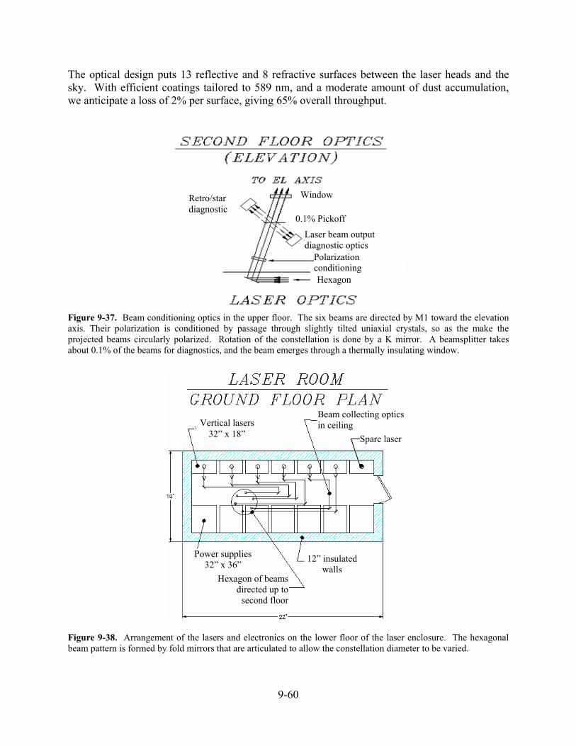
9-60

The optical design puts 13 reflective and 8 refractive surfaces between the laser heads and the sky. With efficient coatings tailored to 589 nm, and a moderate amount of dust accumulation, we anticipate a loss of 2% per surface, giving 65% overall throughput.

Figure 9-37. Beam conditioning optics in the upper floor. The six beams are directed by M1 toward the elevation axis. Their polarization is conditioned by passage through slightly tilted uniaxial crystals, so as the make the projected beams circularly polarized. Rotation of the constellation is done by a K mirror. A beamsplitter takes about 0.1% of the beams for diagnostics, and the beam emerges through a thermally insulating window.

Figure 9-38. Arrangement of the lasers and electronics on the lower floor of the laser enclosure. The hexagonal beam pattern is formed by fold mirrors that are articulated to allow the constellation diameter to be varied.

Retro/star

diagnostic Window

0.1% Pickoff

Hexagon

Laser beam output diagnostic optics

Polarization conditioning

Vertical lasers32” x 18”

Beam collecting optics in ceiling

Power supplies 32” x 36”

Spare laser

Hexagon of beams directed up to

second floor

12” insulated walls

9-61

9.6 AO System, Operation and Overall Performance.

9.6.1 Introduction

A general overview of the sensor and control strategy has been set out in Section 9.4 and in Figure 9-21. In this section we further develop the system aspects and show how the GMT builds on the actual and modeled characteristics of 8 m class AO systems using natural stars and multiple laser beacons for monolithic and segmented telescopes. Thus we explore how the GMT will bring the 8 m segments together as a coherent aperture of 25 m. Unique elements are the very large segment size, the shape of the pupil and its discontinuities, and the use of the one deformable secondary to correct all wavefront errors, including short term motion of the primary segments as well as atmospheric distortion. These aspects are explored in some detail.

Residual errors after adaptive correction of the GMT are relatively straightforward to calculate with a bright star on axis. It is not so easy in LTAO mode, when the wavefront must be reconstructed tomographically from the beacons, and the best available natural guide star is faint and off-axis. The elements of the LTAO system were outlined in Section 9.4. Here we look quantitatively at the performance of all the elements of the LTAO system put together. In this section we account for all the major error terms that were introduced in the performance requirements set out in Section 9.2.

9.6.2 The 8 m Building Blocks

Each of the GMT’s seven 8.4 m primary and corresponding secondary segments can be considered as a powerful 8 m AO system in its own right, with its own 672 actuator deformable secondary and a six-beacon laser constellation for wavefront sensing. Thus when the AO system is turned on, and before any segment co-phasing has been implemented, each segment should perform at the levels being projected for 8 m class telescopes with advanced AO systems. The analysis and experience being developed with monolithic primary mirrors at the MMT, Gemini and the VLT will all be directly applicable to the individual GMT segments.

In our discussion we have already drawn on the experience with a single sodium beacon at Keck. Upcoming development of multi-beacon systems on current 8 m class telescopes will be of particular interest and value. The five Rayleigh beacon system at the MMT, already described, should give closed-loop results on both LTAO and GLAO in the next year or so. In five years time, before the GMT system has to be finalized, there will likely be experience from multi-sodium beacon systems at Gemini and the VLT. The planned implementation at Gemini South has similar parameters to that for the individual GMT segments, with Shack-Hartmann sensor subapertures of 0.5 m and five CW laser beacons of 10 W each. That system is more ambitious in that correction with 3 conjugate deformable mirrors is planned over a 1′ MCAO field, but the wavefront correction on-axis should be similar for the Gemini and GMT single deformable mirror systems. A doubling of laser power will be required at the GMT to offset the Keck-like spot elongation. The main LGS errors for the Gemini system are projected to be 109 nm RMS from fitting error (from the 0.5 m subaperture size), 32 nm RMS from wavefront sensor photon and read noise and 26 nm from servo lag at a sensor frame rate of 800 Hz, close to GMT’s 1 kHz (Ellerbroek et al. 2003). Such performance if proven in practice would validate these error terms for the GMT’s startup AO system.

9-62

Experience with the higher resolution correction possible with the GMTs deformable secondary will be obtained starting in the next year or two with the LBT, and later with the VLT. The LBT shares the same 0.32 m actuator spacing, and will implement correction with pyramid wavefront sensing with the same effective resolution. Correction for bright natural stars at the 120 nm RMS level may thus be validated by this system. The VLT’s planned multiple sodium beacon project, MUSE, aims at correction by an adaptive secondary with 0.25 m subapertures, slightly higher resolution still. This will be a good test of what second generation laser wavefront sensors at the GMT might accomplish. MUSE is a second generation instrument scheduled for operation in 2011. High fidelity correction of the ground layer for improved seeing below 1 μm wavelength is one mode of operation for MUSE that could also be implemented with the GMT beacon constellation. In this mode 4 sodium LGS are set in a square 60″ or 75″ off axis, and high resolution correction is made at 700 Hz frame rate. In worse than average seeing (1.1″) the models project a doubling of the seeing core intensity at 750 nm wavelength over a 1′ field (Hubin et al. 2004).

9.6.3 Bringing the 8 m Segments Together at a Coherent Focus

At the GMT the wavefront from all seven 8.4 m segments is sensed on a single Shack-Hartmann sensor covering the full pupil. Thus the relative tilts across the pupil will be sensed and controlled, whether with natural stars or laser beacons. If no attention were paid to piston errors, then the broadband focus would show an incoherent superposition of the diffraction limited 8 m Airy cores from all seven wavefront segments (Figure 9-39a). Since the long-term differential tilt errors from the Shack-Hartmann sensors are much smaller than the 8 m diffraction limit, in practice the Strehl would be the same as for the individual systems. But if an unresolved star is observed in a short exposure through a narrow band filter, interference will show itself in the form of a triangular pattern of speckles crossing the Airy core. They will show the full pupil resolution, as do speckles at today’s telescopes (Figure 9-39b).

Figure 9-39. Incoherent time averaged K band image, with wavefront control by the full pupil Shack-Hartmann sensor only. a) The ideal 8.4 m Airy pattern. b,c) Narrow band snapshots showing interference speckles, random piston settings. d) Broadband K image with piston values equalized and stabilized. (Square root stretch to show the weaker features.)

To recover the static, coherent full aperture PSF over a broad band (Figure 9-39d), the piston differences between segments must be corrected as follows:

Static set up

a) Set the secondary segments so they form a continuous surface, using optical metrology with an artificial light source.

a b c d

9-63

b) Use starlight piston sensor to measure telescope segment displacements, and remove them by adjusting the primary segments so the speckles are seen in white light.

Operational low frequency control (few Hz)

The primary segment edge sensors will measure differential motions due to telescope structural deformation. Such deformation might be caused by wind gusting, on a time scale of seconds; changing elevation and thermal distortions will cause larger but slower changes. Correct these on short time scale with compensating secondary motions, and by readjusting the primary segments at longer intervals (several minutes).

Operational fast control (kHz)

Corrections to the wavefront shape including tilt and piston terms interpolated across the gaps are sensed at kHz rates optically by the Shack-Hartmann reconstruction and tilt sensors and mechanically by accelerometers. The adaptive secondary will be adjusted to compensate these fast changes. The commands to each secondary segment will include piston motions to ensure continuity of the corrected wavefront across the boundaries.

9.6.4 Static Calibration of Piston of the Primary and Secondary Segments

The deformable secondary is specified so that in operation the shape reference for the deformable surfaces (formed by the segment reference bodies linked to the common subframe) can be trusted not to develop piston differentials >50 nm RMS on time scales of a few minutes, and <2 μm RMS from day to day. The perturbing forces will come from elevation change, temperature changes and wind gusts. If necessary, secondary edge sensors or open loop controls based on elevation will be used to hold these tolerances.

The full seven-segment surface will be calibrated to tolerance of 10 nm RMS by introduction of a retroreflector at prime focus and a metrology unit at the folded Gregorian focus. Details of the calibration system are given in Section 11.3.8.

Once the secondary segments are set to their nominal common surface with the calibrator, the telescope will be pointed to a bright star and the AO control will be turned on, so as to flatten the wavefront segments. The infrared piston sensor will be used, first in capture mode (narrow band filter) to sense the large scale piston errors. These will be removed to better than 1 μm by adjustments to the primary hexapod actuators. At this point the secondary segments can be adjusted to recover the full pupil PSF, and the primary edge sensors will be brought into play.

A conceptual design has been developed for optical sensing of relative tilt and height between primary mirror segments (see Section 8.4.2). The optics will project target images across the gaps between adjacent segments to imaging cameras. The projectors and cameras will be attached to cast bosses on the sides of the primary segments. Two images will be projected, one collimated across the gap, so tilt is sensed, the other passing through an intermediate focus in the gap, so as to sense vertical and lateral shifts. In addition, changes in the gap width will be sensed as changes in focus. The target will consist of a grid (rather than a point), so that the positions of the detected images will be averaged over many CCD detector pixels. In this way, shifts of a

9-64

few nm, much smaller than the 10 μm pixels, will be detectable. On the basis of Keck experience, we estimate the error propagator will be about five, i.e. the wavefront RMS error deduced from the sensor readings will be about five times larger than the individual sensor errors. Thus we expect 5 nm target sensing, and 25 nm RMS wavefront error.

To calibrate the sensors absolutely, primary piston steps will be introduced with the hexapods, and the corresponding secondary segment moved in compensation to recover the full phased pupil PSF, as determined by the interferometric star piston sensor. The secondary calibration source at prime focus will be designed to allow simultaneous operation so that it may be operated during this process, to ensure the secondary surface remains continuous. When the calibration is complete, piston differences measured by the primary edge sensors will be corrected in open loop with the secondary mirror, without adjustments to the primary hexapods on short time scales. Accumulated errors will be off-loaded from the secondaries by primary mirror motions at intervals of a few minutes. Such primary adjustments, which will be accurate to better than 1 μm but not to 20 nm, may involve momentary loss of AO lock. However, the edge sensors will be sensitive to 20 nm RMS motions, and fast responding, so recovery should be possible in a short interval, (<1 s) by feed-forwarding displacement information to the secondary control.

9.6.5 Performance of AO with Natural Guide Stars Only

AO with natural guide stars is the simplest mode of AO operation, and for those applications where a suitable natural star is available will be the mode of choice. Section 9.4.4 gives an analysis of the system sensitivity with a bright star and infrared sensor operating on the coherent beam. In this case, all information for AO control including direct measurement of differential piston errors, comes from the one detector.

9.6.5.1 AO with Shack-Hartmann Sensing of Natural Guide Star

When the NGS wavefront is sensed with the optical NGS Shack-Hartmann sensor, the wavefront across the full pupil will be flattened and tilt corrected, leaving only piston errors between segments. The errors will be no more than half a wave once the correction loop is closed about the primary segment edge sensors. In this case, the interferometric piston sensor described in Section 9.4.3.3, operating in broad-band, will have the sensitivity to recover the piston errors between all the segments unambiguously at the full control speed.

The projected system sensitivity for closed loop operation with the optical Shack-Hartmann sensor and 0.5 m subapertures, is shown in Figure 9-40. For bright stars, the limiting wavefront error for 1 kHz frame rate is 155 nm RMS (S = 0.8 at K), which is dominated by the fitting error (110 nm). For guide stars fainter than 10th magnitude, the degradation due to photon noise is lessened by increasing the integration time. Curves for integration times up to 20 ms are shown. The maximum Strehl ratios and isoplanatic angles as a function of wavelength are given in Table 9-1).

9-65

Figure 9-40. Optical NGS performance with 0.5 m subapertures and 1, 5, 10, and 20 ms integration. The bright star’s RMS residual wavefront error is 155 nm. The atmospheric parameters assumed were r0 = 15 cm and τ0 = 4.3 ms at 0.5 μm.

The same optical sensor, when used to calibrate the LGS sensors, will need an integration time of ~1 minute to reach a faint field star. We suppose a limit of R = 19, which will give an 80% probability of finding a star within 1′ at the Galactic pole. The photon flux over 600–900 nm bandwidth will be ~250 photons/m2/s. The appropriate long term FWHM of the spots is set by normal seeing, which we take as 0.7″. We would like to measure the time average slopes to 0.02″ RMS error, to be more accurate than the laser measurement. Following the same estimation procedure described in Section 9.6.6.1 below for the LGS mode, and assuming negligible read and sky noise, we find the required photoelectron count is 600, which will require an integration time of 24 s, set by photon noise. This is commensurate with the integration time of ~1 minute needed to average out atmospheric errors arising from anisoplanatism.

9.6.6 LTAO: Tomographic Reconstruction of Shack-Hartmann Data

The Shack-Hartmann sensors used to measure the laser beacon wavefronts are described in Section 9.4.2.1 above. Here we estimate the expected errors in the tomographically reconstructed wavefront, in addition to the fitting error, which is 121 nm in median seeing from the 49.4 cm subaperture size.

Extensive modeling of tomographic reconstructors for apertures up to 32 m has been made by Ellerbroek (2004). The atmospheric parameters he adopted were similar to the median values for Las Campanas listed in 9.2, except for a more favorable value of τ0 (0.5 μm) of 4.9 ms vs. our 2.5 ms. The subaperture size of 50 cm was very close to our 49.4 cm, and the beacon constellation was similar, 5 beacons on a 2′ diameter vs. our six on 1.3′ diameter. Ellerbroek’s result for 25 m aperture is a reconstructed wavefront error of 155 nm RMS. The major contributors are fitting error, temporal lag error for a 700 Hz frame rate, and noise in the Shack-Hartmann spot measurement of 0.02″.

The GMT project has not yet completed a full tomographic reconstruction model for the GMT pupil at a corresponding level of sophistication, but our own projection, based on our assessment of the component terms, is in good agreement.

9-66

9.6.6.1 Photon Noise

For the GMT, the contribution due to photon noise in the slope measurements is estimated as follows. The baseline power for each laser is 30 W, with a projected uplink transmission of 65%, giving 20 W at the beam projector. The return path has optical losses which we estimate will lead to an overall 40% effective quantum efficiency. (These losses include the primary and secondary mirrors, the middle dichroic in transmission and the low one in reflection, the narrow band 589 nm transmission dichroic that reflects away the calibration NGS, the relay optics, the lenslet array and the CCD). The estimated signal from the measured typical return from a CW laser of 1.2×106/m2/J (Ge et al. 1998) is 2,400 photoelectrons per subaperture per ms, half this for low column density. This count corresponds to an average flux of 100 photoelectrons over each of the 25 pixels in each subaperture, for an RMS photon noise average of 10 e- RMS. Since the slope signal will be derived from the brighter pixels, the read noise of 3 e- RMS will be negligible. In this limit, the subaperture slope error is given by 0.7(FWHM)/√N (Sandler et al, 1994). The effective FWHM is taken to be 2″ for the radial direction, which is appropriate for subapertures at the pupil edge, assuming advantage has been taken of cross correlation methods on radial structure. On this basis we find a slope error σθ = 0.028″ RMS under typical column density, and 0.040″ when the column density is low. The resulting noise term for the reconstructed wavefront is given by Gσθd, where d is the subaperture dimension and G a noise propagation parameter, which is approximately unity for multiple beacon reconstructors (Sandler 1999). For G = 1, we find the error contribution for a single wavefront sensor for average column density of 68 nm RMS and 100 nm for low column density. When all six wavefront sensors are combined tomographically, the errors are reduced to 28 nm and 40 nm RMS.

9.6.6.2 Effect of Segment Gaps on the Reconstruction

The error in the tomographic reconstruction from residual effects of focus anisoplanatism is likely to be similar to the continuous filled aperture modeled by Ellerbroek, except for the effect of the segment gaps. These are bridged by the reconstruction with full aperture modes. To explore what piston errors might arise, we have built a Shack-Hartmann reconstructor explicitly for the GMT pupil. For simplicity, the input slopes were for a single NGS wavefront measured with the 49.4 cm subaperture geometry over the full pupil, not for the full tomographic set of six beacons. (Piston error may well be smaller for the tomographic solution, which does in fact sense across the gaps for layers higher than 2 km). The reconstructor uses a basis set derived from sinusoidal modes, orthogonalized over the GMT pupil. The reconstructor is not yet fully optimized, but it already is finding that the piston error caused by the gaps is not large.

The left panel of Figure 9-41 shows an example of a modeled input wavefront, with r0 = 15 cm and outer scale 25 m. The RMS error across the full pupil after subtraction of the reconstruction of this wavefront is shown in the right panel, to the same scale as the input. Figure 9-42 shows a typical set of slopes across the subapertures that are the inputs to the reconstructor.

9-67

Figure 9-41. (Left) Single realization of atmospheric wavefront across the GMT pupil from a distribution with r0=15 cm and outer scale 25 m. (Right) Residual error after subtraction of full aperture wavefront reconstructed from the slope data of Figure 9-42.

Time sequences showing the evolution over time of piston differences of the uncorrected wavefront and the residual piston errors after subtraction of the reconstructed wavefront are shown in Figure 9-43 and Figure 9-44. The uncorrected pistons are the terms that must be applied to the deformable secondary segments. The RMS of the individual piston motions is 4 μm. The RMS piston error after subtraction of the reconstructed wavefront in this example is 90 nm RMS. At this level the residual is a significant but not dominant contribution to the total error budget. On the basis of additional modeling, we project that for a fully optimized GMT reconstructor the piston error will be halved to 50 nm rms.

Figure 9-42. Wavefront slopes for simulation in Figure 9-41 that are the inputs for the Shack-Hartmann reconstruction.

9-68

Figure 9-43. Evolution over 1 s of segment-averaged piston motions for the modeled atmospheric wavefront, with r0 = 15 cm and τ0 (0.5 μm)= 2 ms. These are representative of the atmospheric component of piston motions that must be applied to the seven deformable secondary segments. The piston velocities are typically 20 μm/s, and the accelerations are 50 μm/s2, less than 10-5 g.

Figure 9-44. Seven piston residuals after correction by Shack-Hartmann reconstruction of the full pupil. The RMS error is 90 nm.

9.6.7 LTAO: NGS Measurements

In the LTAO mode, fast tilt measurements and piston error calibration must be measured from a faint natural star off-axis. The performance is limited if the best available star is either too faint, in which case photon or sky noise enters, or else too far off-axis, in which case anisoplanatism limits the accuracy of the measurement. We examine here how these limits apply to the GMT, focusing on the limits that are peculiar to this telescope.

9.6.7.1 Field Star Statistics

The density and probability for finding field stars can be derived from the convenient summary in a chart for R band magnitude limits by Roddier (1999). This shows that at the Galactic pole we must search out to 60″ radius to find a star of R magnitude 19 or brighter with probability

9-69

80%. The corresponding H magnitude for typical field stars, giants of spectral type K5, is 16.8, and 16.6 in K band. We found in Section 9.4.3.2 that the photon counting tip-tilt sensor would have sensitivity limited by photon noise to 1.6 mas RMS in 1 ms for H = 17. Thus the probability of finding a field star of this magnitude at the Galactic pole is >80%.

9.6.7.2 Tilt Anisoplanatism

We are concerned with tilt anisoplanatism, which limits the accuracy of fast tip-tilt measurements as off-axis angle is increased, and piston anisoplanatism, which limits the accuracy of instantaneous segment piston differences measured with an off-axis star.

The RMS image motion due to tilt anisoplanatism in the radial and tangential directions for Kolmogorov turbulence (with no outer scale of turbulence) is given in terms of r0 and the isoplanatic angle θ0 by

σθ = k λD

θθ0

Dr0

⎛

⎝ ⎜

⎞

⎠ ⎟

−1/ 6

Equation 9-5

where k = 0.22 for motion in the x direction and 0.13 for the y direction (Sandler et al. 1994). We see that for given angular separation the motion as a fraction of the diffraction width gets smaller with increasing telescope diameter D, but only as the -1/6 power. However, for the GMT the effect of outer scale of turbulence must be included, since the telescope diameter is of comparable scale. The result is favorable, in that anisoplanatism is less than would be the case for Kolmogorov turbulence, and thus the tilt motion relative to the diffraction limit becomes smaller.

The CAOS simulation package (Carbillet et al. 2001) has been used to model this effect for the GMT. Model atmospheres with specific strengths of turbulence as a function of height were taken from the detailed measurements at Cerro Pachón. Two vertical profiles for Cn

2 were used, to represent typical and good seeing (r0 = 14 cm, θ0 = 2.10″ and r0 = 18 cm, θ0 = 2.38″ respectively, all at 0.5 μm wavelength), and results were calculated for outer scales of 25 m and infinity. The results for tilt anisoplanatism are shown in Figure 9-45.

The numerical model for infinite outer scale is in reasonable agreement with the analytical formula. For an angular separation of 60″, Equation 9-5 yields a combined RMS motion (for either of the two orthogonal directions) of 13 mas and 12 mas for typical and good seeing motions respectively, compared to 10 and 9.5 mas for the model. However, when the typical outer scale of 25 m is included, the tilt anisoplanatism is halved to ~5 mas. This means that the GMT is at a huge advantage compared to 8 m class telescopes. The field available to find stars sharing motion to a given fractional limit is approximately doubled, and thus the probability of finding a star to a given magnitude limit is quadrupled.

The increased anisoplanatic angle, higher sensitivity because of higher photon flux and less sensitivity to sky background combine to give the GMT an >80% probability of finding a highly viable guide star with ≤ 5 mas RMS tip/tilt error at any point on the sky.

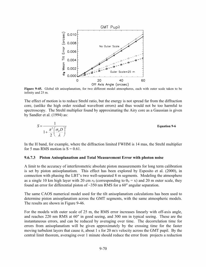
9-70

Figure 9-45. Global tilt anisoplanatism, for two different model atmospheres, each with outer scale taken to be infinity and 25 m.

The effect of motion is to reduce Strehl ratio, but the energy is not spread far from the diffraction core, (unlike the high order residual wavefront errors) and thus would not be too harmful to spectroscopy. The Strehl multiplier found by approximating the Airy core as a Gaussian is given by Sandler et al. (1994) as:

S =1

1+π 2

2σθ D

λ⎛ ⎝ ⎜

⎞ ⎠ ⎟

2 Equation 9-6

In the H band, for example, where the diffraction limited FWHM is 14 mas, the Strehl multiplier for 5 mas RMS motion is S = 0.61.

9.6.7.3 Piston Anisoplanatism and Total Measurement Error with photon noise

A limit to the accuracy of interferometric absolute piston measurements for long term calibration is set by piston anisoplanatism. This effect has been explored by Esposito et al. (2000), in connection with phasing the LBT’s two well-separated 8 m segments. Modeling the atmosphere as a single 10 km high layer with 20 cm r0 (corresponding to θ0 = x) and 20 m outer scale, they found an error for differential piston of ~350 nm RMS for a 60″ angular separation.

The same CAOS numerical model used for the tilt anisoplanatism calculations has been used to determine piston anisoplanatism across the GMT segments, with the same atmospheric models. The results are shown in Figure 9-46.

For the models with outer scale of 25 m, the RMS error increases linearly with off-axis angle, and reaches 220 nm RMS at 60″ in good seeing, and 300 nm in typical seeing. These are the instantaneous errors, and can be reduced by averaging over time. The decorrelation time for errors from anisoplanatism will be given approximately by the crossing time for the faster moving turbulent layers that cause it, about 1 s for 20 m/s velocity across the GMT pupil. By the central limit theorem, averaging over 1 minute should reduce the error from projects a reduction

9-71

by √60, i.e. from 220 nm RMS (at 60″) to 30 nm RMS. Thus 1 minute integrations should be completely satisfactory for calibration.

Figure 9-46. Anisoplanatism for differential piston measurement made with an off-axis star.

The wavelength for piston measurements should be long enough so that the instantaneous piston fluctuations from anisoplanatism are ≤1 radian, so that the averaging can be simply by integration of the interference images on the detector array. K band should be satisfactory for 1′ field angle, with 300 nm instantaneous error in typical seeing corresponding to 1 radian, not enough to wash out the contrast of the diversity images.

The total error in the 1 minute integrations must include the term from photon noise. If we suppose the same the K = 17 guide star is divided with a beamsplitter into 90% for tilt and 10% for the piston sensor, the total detected photoelectron flux from the piston sensor will be ~105 photoelectrons. This flux will be detected over the two phase diverse images, each with about 100 pixels. The average count per pixel will thus be 500, and the photometry per pixel will be good to 5% as long as the read noise is <10 e- RMS. We have not yet calculated the noise propagator for the piston solution. However, it is likely that at this level of photometry, the piston errors will be larger than the 25 nm time averaged anisoplanatism, but still below an acceptable 50 nm RMS level. Otherwise, longer integrations for calibration will be required.

We note that for AO correction of the L band, tilt anisoplanatism will be acceptable to 2′ radius. For this reason, we required the field for infrared tilt and piston stars for the GMT to be 4′ diameter. The larger field may be of value also at shorter wavelengths for spectroscopy, when a larger aperture for high encircled energy is used. Tilt anisoplanatism of 8 mas RMS at 2′ off-axis would not cause much loss of energy in a 0.03″ wide slit.

9.6.8 LTAO: Start Up, Capture and Operation

The sequence of operations for a cold start to diffraction limited LTAO will be as follows:

9-72

1) Set deformable secondary to continuous 3 m parent surface (zero piston errors). Metrology to do this during the day will be by insertion of reflector at prime focus and double pass white light interferometer at the Gregorian focus.

2) Use laser trackers to get primary segment pistons within 100 μm in six degrees of freedom. Each segment will have three fixed reflectors referenced to the surface during manufacture. The trackers will be near the secondary.

3) Point to bright star on axis and bring 8 m individual AO systems into operation without regard to piston.

4) Run AO system now with piston changes interpolated by full pupil reconstructor.

5) With narrow band filter and fast IR camera look at interference in 8 m diffraction core – at this point the interference pattern becomes stable.

6) Correct piston path differences. This will be done by the Chanan method of exploring visibility, in this case by pistoning the adaptive secondary segments. The errors are reduced by moving the primary segments by their hexapods and progressing to broader band and shorter wavelength. When the errors are nulled the primary segment edge sensor readings will be recorded.

7) Switch to stars at different elevation, and show that differential displacements measured by primary edge sensors can be corrected in open loop by secondary deformations.

8) Check that field star sensors give correct fast tilt and slow piston values. Tilt measured from field star should be applied as full rigid body motion of adaptive secondary.

9) For LTAO mode, turn on the laser beacon tomography system with a field star providing fast tip-tilt and slow piston, and fast piston from edge sensors. Verify that the tomographically reconstructed wavefronts agree with that measured for a field star on axis (this is the stage now reached with the MMT multi-beacon system, though without the complication of a segmented wavefront).

10) Point the GMT to a starburst galaxy at z = 1.4, Lock on the LTAO beacon correction, then also lock tilt on the field star at 1 arcminute radius. Integrate for an hour with the narrowband H filter in HRCam, with calibration of piston and laser wavefront every minute from the same tilt star, to obtain the image shown in Figure 9-1.

9.7 Real-time Reconstructor

A reconstructor for the GMT AO system must be capable of reconstructing the wavefront from the wavefront slopes in order to update the deformable mirror’s 4620 actuators every millisecond. The size of the computational problem is challenging: with the LGS in operation, the Shack-Hartmann sensor for each beacon has 1500 subapertures. For a continuous deformable mirror, the reconstructor matrix would then naively have 18000×4620 elements. On each iteration, wavefront reconstruction with a fully-populated matrix would require 8×107

9-73

floating point operations. The real-time computer would have to be capable of sustained calculation at a minimum of 100 GFlop.

For the GMT, though, there is no coupling of actuator influences across the segment boundaries. The wavefront reconstruction can be conceptually broken into two pieces: the first recovers the 8.4 m pieces of wavefront across each of the segments independently, and the second estimates those few low-order modes across the full 24.4 m pupil that contribute significantly to the atmospheric piston errors. The computational demand is therefore reduced by a factor of seven, since actuators on a given secondary segment are driven almost entirely by Shack-Hartmann slopes measured within the same segment. In fact, each segment needs less computing power than the Gemini MCAO system, which must drive three DMs (instead of one) from five laser beacons sensed with about the same sampling in the pupil as GMT.

The real-time computer must run at ~15 GFlop sustained throughput, which would not be particularly difficult to construct even today. The MMT tomographic system will be driven by a computer built by Microgate, which is designed to accept up to 1500 WFS slope inputs, and drive the MMT’s 336-actuator ASM at 1 kHz frame rate. It is capable of sustained calculation at ~1 GFlop, and is a small unit, easily fitting into a single bay of a standard 19 inch rack. It is designed around custom boards, with computation handled by floating point DSPs, and high-speed communication handled by large FPGAs. It is a readily expandable architecture which we adopt for GMT, anticipating that it will be implemented with upgraded hardware to be expected on the timescale of the telescope’s construction.

9.8 Optical System for AO Wavefront Sensors and AO Instruments

The system of dichroics and field probes for separation of the science instruments and AO wavefront sensing functions has been outlined above in Section 9.1.5. Here we give more details of the system and its components.

9.8.1 Wide field Optical AO System

The low dichroic mirror (Figure 9-4) on a CaF2 substrate is located at the level of the platform floor, 70 cm above the Gregorian focus. It transmits 1-2.5 μm to wide field imagers or spectrographs at the direct Gregorian focus. The aberration of the transmitted beam caused by transmission through the tilted plate is corrected by figuring the underside of the substrate with slight cylinder. The mirror is angled at 25° incidence and reflects the optical light in the 8′ field needed for GLAO toward the LGS and NGS optical sensors, kept clear of the incoming 8′ beam.

The sensor assembly is shown in Figure 9-47. Three optical tip-tilt sensors are located on probes that move across the infinity focal surface to pick up field stars. They will be constrained to move within the six wedges defined by the footprint of the LGS light at the infinity focal plane (Figure 9-48) where they will not obscure any part of the beacon pupils. The sodium beacon focal surface lies from 20 to 40 cm further back, corresponding to 90 to 180 km range (elevation down to 30°). Here, a six-armed radial assembly supports the six Shack-Hartmann sensors. The whole assembly rotates about its axis to counter the effect of the telescope’s field rotator, keeping the individual sensors pointed at their corresponding beacons and preserving the mapping of each sensor onto the actuators of the adaptive secondary. The sensors are also

9-74

individually articulated to move both radially 24 cm (out to 4′ radius) and axially over 20 cm. A full resolution optical Shack-Hartmann sensor for NGS will be fed via a 589 nm notch transmitting dichroic behind the focal plane, so it can be set anywhere within a 3′ diameter field while the lasers are set out to 2′ diameter with no pupil vignetting. When the telescope is to be used for direct imaging with no AO over a field of view up to 24′ in diameter, the dichroic and sensor unit is translated to the right to clear the beam completely.

9.8.2 Relay Optics to near IR AO Instruments and Wavefront Sensors

In order for IR AO instruments operating at the diffraction limit to share the same optical wavefront sensing unit, they will be fed by dichroic mirrors located higher up in the beam. The first of these (the middle dichroic in Figure 9-4) will be used to feed both the IR wavefront sensors and the JHK science instruments. It has the reverse reflection characteristic to the lower dichroic, transmitting the optical through to the optical sensor, and reflecting the J, H and K bands. The central 1′ field passing by these sensor probes is relayed via an Offner relay to science instruments (Figure 9-6). To improve performance, the angle of incidence on this dichroic is chosen again to be as small as possible, 25°, consistent with throwing the reflected beam clear so that the wavefront sensor unit (which is in vacuum) can remain in place without vignetting the 24′ diameter direct Gregorian feed. A preliminary design for this dichroic is shown in Figure 9-49. It achieves an average of 98% reflectivity from 1.1-2.5 µm, while transmitting >80% at 589 nm.

Figure 9-47. Optical wavefront sensor package. The laser beacon sensors are on radial and axial stages, and are shown positioned at 2′ diameter and at the inner (180 km) focus (blue rays). The sodium images are formed ahead of the optical assemblies that relay the light to the sensors. Three STRAP tip-tilt units are shown fed by small pickoff mirrors in the infinity focal plane. In addition, to the right is a full resolution Shack-Hartmann sensor fed by a removable 589 notch dichroic that reflects a 3′ NGS field and transmits a laser beacon constellation of 2′ diameter.

9-75

Figure 9-48. Footprint of sodium beacons at 90 km on infinity focal plane where the NGS tip-tilt sensor probes are located. The radii are shown from the closest, 40″ radius, in dark blue to the widest, 4′ radius.

Figure 9-49. Preliminary design for the middle dichroic at 25° incidence to reflect JHK (blue) to the diffraction limited science instruments and transmit optical (red) through to the optical sensor unit.

At the 4′ bent Gregorian focus inside the dewar will be the near-IR pyramid (PRWFS) sensor to provide full wavefront sensing for those targets for which a convenient brighter NGS is available. It will serve also as the first-stage sensor for ExAO. The sensor will be fed with a choice of a probe mirror or one of two 1′ dichroics which allow it to share light by wavelength division with a bright on-axis science target. Three other probes across the 4′ field will be used to feed tip-tilt and phase sensors to be used in conjunction with the LGS sensors fed from the low dichroic. The reason for such a large field is that when the guider is used for longer wavelengths, the isoplanatic patch increases to be this big.

The Offner relay gives diffraction limited images over 1′ relayed to f/15. Spot diagrams are shown in Figure 9-50. The design includes an atmospheric dispersion corrector placed in the f/15 beam rising up to the instrument selector mirror. The design has two zero-deviation prisms of zinc sulphide and zinc selenide whose dispersions are well balanced for this compensation. The prisms are each 280 mm diameter with ½ degree wedge angle and achromatize images to the diffraction limit over the J, H, and K bands and the full elevation range of the telescope.

9-76

Figure 9-50. Spot diagrams for the Offner corrector. All three panels show spots over the 1′ field displaced up and down and left and right by 20″, 40″ and 60″ from the axis. The upper set is for zenith pointing, middle set for 45° elevation showing atmospheric dispersion and the bottom set with the ZnS-ZnSE ADC in place. The circles are the dark Airy ring for 1.25 µm wavelength.

9-77

Because this correction is made after the wavefront sensor pickoffs, the sensors will include additional small individual atmospheric dispersion correctors. A nice feature of the Offner design is that the image of the pupil formed on the second (convex) mirror has very little anamorphic distortion of only 0.6%, thus the rotating cold pupil stop at this location will work very well (Figure 9-51). Figure 9-52 shows the Offner relay and IR wavefront sensor on the rotating platform.

Figure 9-51. Footprint of the pupil on the Offner secondary mirror, where a cold rotating pupil stop will be located, and possibly also a fast steering mirror.

Figure 9-52. IR wavefront sensor and Offner relay dewar on the rotating platform, shown being fed by the middle dichroic.

9.8.3 Relay for Thermal IR Instruments

Instruments operating in the thermal infrared will be served by two interchangeable dichroics that reflect just the longer wavelengths and transmit the optical and near infrared. They will be inserted above the two wavefront sensor-feeding dichroics. These top dichroics will be angled at 30° incidence, so the reflected beam comes clear of the 24′ wide field and is then folded down within the 2 m clearance above the platform. Different thermal infrared instruments can thus be located permanently on the platform, and the upper dichroic will be inserted and rotated as required. The entrance windows to these instruments are tilted down at 30° to the vertical. One dichroic, with a single very high reflectance stack will be used to reflect the L and M bands (3.4–

9-78

5.1 μm). Figure 9-53 shows the result of an early investigation into the dielectric stack required for this dichroic.

The second dichroic, illustrated by the reflectance and transmission curves of Figure 9-54, will be used for longer wavelengths (λ>8 µm). Reflectivity is excellent in the science bands, while the transmission peaks at 70% in the J band. Further work is needed to find the optimal layer stack to improve transmission in the near IR to feed the wavefront and tip-tilt-piston sensors.

Figure 9-53. Preliminary reflectance and transmission characteristics for the dichroic for L and M band science instruments. Good transmission is obtained shortward of 1 μm, and at J, H, and K. Very high reflectivity is exhibited in the thermal science bands.

Figure 9-54. Early investigation into a dichroic optimized for high reflection from 8 to 25 μm with as much optical and near IR transmission as possible. Two thin silver layers provide the broadband IR reflection. Transmission peaks at 70% in J band.

9-79

When an upper dichroic is introduced, the transmitted beam at shorter IR wavelengths is aberrated by transmission through the filter substrate. To maintain diffraction limited imaging performance for the near IR sensors when the mid IR dichroic is in place, an additional compensating plate will be inserted ahead of the near IR focus.

9.9 References

Andersen, D. R. et al. 2006, “Performance Modelling of a Wide Field Ground Layer Adaptive Optics System,” submitted to PASP

Angel, J. R. P., Wizinowich. P. L., Lloyd-Hart, M., & Sandler, D. G. 1990, “Adaptive Optics for Array Telescopes using Neural Network Techniques,” Nature, 348, 221

Angel, J. R. P. 1992, “Use of Natural Stars with Laser Beacons for Large Telescope Adaptive Optics,” Proc. Laser Guide Star Adaptive Optics Workshop, Kirtland AFB, Albuquerque, 2, 494

Angel, J. R. P. 1994, “Ground-Based Imaging of Extrasolar Planets Using Adaptive Optics,” Nature, 368, 203

Angel, J. R. P. 2003, “Imaging Exoplanets from the Ground,” ASP Conference Series, 294, 543

Angel, J.R.P., Lloyd-Hart, M., Codona, J., & Johns, M. 2005 “The Giant Magellan Telescope: 24 m Aperture Optimized for Adaptive Optics,” AMOS Technical Conference, to be published

Audley, M. D. et al. 2004, “Modeling the Electromagnetic Properties of the SCUBA-2 Detectors,” Proc. SPIE, 5498, 416

Beckers, J. M. 1988, “Increasing the Size of the Isoplanatic Patch with Multiconjugate Adaptive Optics,” in Very Large Telescopes and their Instrumentation, ed. M.-H. Ulrich, (Garching: ESO), 2, 693

Berkefeld, T., Soltau, D., & von der Lühe, O. 2005, “Results of the Multi-Conjugate Adaptive Optics System at the German Solar Telescope, Tenerife,” Proc. SPIE, 5903, 180

Bouchez, A. H. et al. 2004, “Keck Laser Guide Star Adaptive Optics: Science Verification Results,” Proc. SPIE, 5490, 321

Burrows, A., Sudarsky, D., & Hubeny, I. 2004, “Spectra and Diagnostics for the Direct Detection of Wide-Separation Extrasolar Giant Planets,” ApJ, 609, 407

Carbillet, M., Fini, L., Femenía, B., Riccardi, A., Esposito, S., Viard, É., Delplancke, F., and Hubin, N. 2001, “CAOS Simulation Package 3.0: an IDL-based Tool for Adaptive Optics Systems Design and Simulations,” ASP Conf. Proc., 238, 249

Carbillet, M., Vérinand, C., Esposito, S., Riccardi, A., Puglisi, A., Femenía, B., & Fini, L. 2003, “Performance of the First-Light Adaptive Optics System of LBT by Means of CAOS Simulations,” Proc. SPIE, 4839, 131

9-80

Chanan, G. & Pintó, A. 2004, “Efficient Method for the Reduction of Large Piston Errors in Segmented-Mirror Telescopes,” Proc. SPIE, 5382, 422

Chauvin, G. et al. 2004, “ A Giant Planet Candidate Near a Young Brown Dwarf,” Astron. Astrophys. Lett., 425, L29

Close, L. M. et al. 2003, “Mid-Infrared Imaging of the Post-AGB Star AC Herculis with the MMT Adaptive Optics System,” ApJ Lett, 598, L35

Close, L. M. et al. 2005, “A Dynamical Calibration of the Mass-Luminosity Relation at Very Low Stellar Masses and Young Ages,” Nature, 433, 286

Codona, J. L. & Angel, J. R. P. 2004, “Imaging Extrasolar Planets by Stellar Halo Suppression in Separately-Corrected Color Bands,” ApJ Lett, 605, L117

Codona, J. L. & Angel, J. R. P. 2006, “Limiting Sensitivity for Ground-Based Detection of Exoplanets,” in preparation

Colucci, D. & Angel, J. R. P. 1992, “Stellar Phase Shifting Interferometer,” OSA Conference on Adaptive Optics for Large Telescopes, Technical Digest Series 19, 124

Costa, J. B. et al. 2004, “Status Report of PYRAMIR: a Near-Infrared Pyramid Wavefront Sensor for ALFA,” Proc. SPIE, 5490, 1189

Dekany R. G. et al. 2004, “Adaptive Optics Requirements Definition for TMT,” Proc. SPIE, 5490, 879

De La Rue, I. & Ellerbroek, B. L. 2002, “Multiconjugate Adaptive Optics with Hybrid Laser Beacon Systems,” Proc. SPIE, 4494, 290

Drummond, J., Telle, J., Denman, C., Hillman, P., Spinhirne, J., and Christou, J. 2004, “Sky Tests of a Laser-Pumped Sodium Guidestar With and Without Beam Compensation,” Proc. SPIE, 5490, 12

Ellerbroek, B. L. et al. 2003, “MCAO for Gemini-South,” Proc. SPIE, 4839, 55

Ellerbroek, B. L. 2004, “Wave-Front Reconstruction Algorithms and Simulation Results for Multi-Conjugate Adaptive Optics on Giant Telescope,” Proc. SPIE, 5382, 478

Ellerbroek, B. L. 2004, Presentation at the Center for Adaptive Optics Fall Retreat, November 13

Esposito, S., Riccardi, A., & Femenía, B. 2000, “Differential Piston Angular Anisoplanatism for Astronomical Optical Interferometers,” A&A Lett., 353, L29

Esposito, S. et al. 2003, “Development of the First Light AO System for the Large Binocular Telescope,” Proc. SPIE, 5169, 149

Esposito, S., et al. 2004, “Integration and Test of the First Light AO system for LBT,” Proc. SPIE, 5490, 228

9-81

Finger, G. et al. 2004, “Performance Limitations of Small Format High Speed Infrared Arrays for Active Control Loops in Interferometry and Adaptive Optics,” Proc. SPIE, 5499, 97

Fugate, R. Q. et al. 1999, “Adaptive Optics for the 21st Century,” ASP Conference Series, 174, 55

Fugate, R. Q. et al. 2004, “Progress Toward a 50-watt Facility-Class Sodium Guide Star Pump Laser,” Proc. SPIE, 5490, 1010

Ge, J., Jacobsen, B. P., Angel, J. R. P., McGuire, P. C., Roberts, T., McLeod, B. & Lloyd-Hart, M. 1998, “Simultaneous Measurements of Sodium Column Density and Laser Guide Star Brightness,” Proc. SPIE, 3353, 242

Geary, J. G. et al. 2005, “The LSST Sensor Development Program,” AAS Meeting 207, 2619

Gendron, E. et al. 2003, “NAOS Infrared Wave-Front Sensor Design and Performance,” Proc. SPIE, 4839, 195

Ghedina, A. et al. 2003, “On Sky Test of the Pyramid Wavefront Sensor,” Proc. SPIE, 4839, 869

Guyon, O. 2005, “Limits of Adaptive Optics for High-Contrast Imaging,” ApJ, 629, 592

Hinz, P. M. et al. 2004, “Large Binocular Telescope Interferometer: the Universal Beam Combiner,” Proc. SPIE, 5491, 787

Hubin, N., Le Louarn, M., Conzelmann, R., Delabre, B., Fedrigo, E. & Stuik, R. 2004, “Ground Layer AO correction for the VLT MUSE project,” SPIE Proc., 5490, 846

Langlois, M. et al. 2004, “Solar Multiconjugate Adaptive Optics at the Dunn Solar Telescope: Preliminary Results,” Proc. SPIE, 5490, 59

Liu, W. M. et al. 2005, “Resolved Mid-Infrared Emission around AB Aurigae and V892 Tauri with Adaptive Optics Nulling Interferometric Observations,” ApJ Lett, 618, L133

Lloyd-Hart, M. et al. 1992, “First Results of an on-line Adaptive Optics System with Atmospheric Wavefront Sensing by an Artificial Neural Network,” ApJ Lett, 390, L41

Lloyd-Hart, M. et al. 1993, “Direct 75 Milliarcsecond Images from the Multiple Mirror Telescope with Adaptive Optics,” ApJ Lett, 402, L81

Lloyd-Hart, M. et al. 1998, “First Astronomical Images Sharpened with Adaptive Optics using a Sodium Laser Guide Star,” ApJ, 493, 950

Lloyd-Hart, M. & Milton N. M. 2003, “Fundamental Limits on Isoplanatic Correction with Multiconjugate Adaptive Optics,” JOSA A, 20, 1949

Lloyd-Hart, M. et al. 2005, “First tests of wavefront sensing with a constellation of laser guide beacons,” ApJ, 634, 679

9-82

Molodij, G. & Rousset, G. 1997, “Angular Correlation of Zernike Polynomials for a Laser Guide Star in Adaptive Optics,” Optical Society of America, 14, 8, 1949

Neyman, C. 2004, “Atmospheric Parameters for Manuna Kea,” Keck Adaptive Optics Note #303, 1

Poyneer, L. A. & Véran, J.-P. 2005, “Optimal Modal Fourier-Transform Wavefront Control,” JOSA A, 22, 1515

Ragazzoni, R. & Farinato, J. 1999, “Sensitivity of a Pyramidic Wave Front Sensor in Closed Loop Adaptive Optics,” A&A Lett., 350, L23

Ragazzoni, R., Marchetti, E., & Rigaut, F. 1999, “Modal Tomography for Adaptive Optics,” A&A Lett., 342, L53

Rhoadarmer, T. A. et al. 1999, “Laboratory Adaptive Optics System for Testing the Wavefront Sensor of the New MMT,” Proc. SPIE, 3762, 161

Riccardi, A., Brusa, G., Salinai, P., Gallieni, D., Biasi, R., Andrighettoni, M., & Martin, H. M. 2002, “Adaptive Secondary Mirrors for the Large Binocular Telescope,” Proc. SPIE, 4839, 721

Riccardi, A., Biasi, R., Brusa, G., Del Vecchio, C., Esposito, S., Gallieni, D. & Salinari, P. 2003, “Giant Segmented Adaptive Mirrors: progress report,” SPIE Proc., 4840, 246

Riccardi, A. et al. 2004, “The Adaptive Secondary Mirrors for the Large Binocular Telescope: a Progress Report,” Proc. SPIE, 5490, 1564

Roddier, F. 1999, Adaptive Optics in Astronomy, ed. F. Roddier, ch. 3, Theoretical aspects, p. 55, (Cambridge:CUP)

Romani, R. W., Miller, A. J., Carrera, B., Nam, S. W., & Martinis, J. M. 2001, “Phase-Resolved Crab Studies with a Cryogenic Transition-edge Sensor Spectrophotometer,” ApJ, 563, 221

Rosenberg, D., Lita, A. E., Miller, A. J., & Nam, S. 2005, “Noise-Free High-Efficiency Photon-Number-Resolving Detectors,” Phys. Rev. A, 71, 061803-1

Sandler, D.G., Stahl, S., Angel, J.R.P., Lloyd-Hart, M., and McCarthy, D. 1994, “Adaptive Optics for Diffraction-Limited Infrared Imaging with 8 m Telescopes,” Journal of the Optical Society of America A, 11, 925

Sandler, D. G. 1999, Adaptive Optics in Astronomy, ed. F. Roddier, ch. 12, The design of laser beacon AO systems, (Cambridge: CUP)

She, C. Y. et al. 2000, “Eight-Year Climatology of Nocturnal Temperature and Sodium Density in the Mesopause Region (80 to 105 km) over Fort Collins, CO (41º N, 105º W),” Geo. Res. Lett. 27, 3289

9-83

Spinhirne, J.M. et al. 1998, “The Starfire Optical Range 3.5m Telescope Adaptive Optical System,” SPIE Proc., 3353, 22

Stahl, S. M. & Sandler, D. G. 1995, “Optimization and Performance of Adaptive Optics for Imaging Extrasolar Planets,” ApJ Lett, 454, L153

Tokovinin, A., Le Louarn, M., & Sarazin, M. 2000, “Isoplanatism in a Multi-Conjugate Adaptive Optics System,” JOSA A, 17, 1819

Tokovinin, A., Le Louarn, M., Viard, E., Hubin, N., & Conan, R. 2001, “Optimized Modal Tomography in Adaptive Optics,” A&A, 378, 710

van Dam, M. A., Le Mignant, D., & Macintosh, B. A. 2004, “Performance of the Keck Observatory Adaptive-Optics System,” App. Opt., 43, 29

Wildi, F. et al. 2002, “First Light of the 6.5-m MMT Adaptive Optics System,” Proc. SPIE, 5169, 42

Wizinowich, P. L. et al. 2004, “Adaptive Optics Developments at Keck Observatory,” Proc. SPIE, 5490, 1

Wizinowich, P. L. et al. 2006, “The W. M. Keck Observatory Laser Guide Star Adaptive Optics System: Overview,” PASP, in press