8thInternationalWorkshoponDataMininginBioinformatics

(BIOKDD2008)

Held in conjunction with SIGKDD conference, August 24, 2008

WorkshopChairs

Stefano Lonardi Jake Y. Chen

Mohammed Zaki

BIOKDD ʻ08: 2008 International Workshop on Data Mining in Bioinformatics

Las Vegas, NV, USA Held in conjunction with

14th ACM SIGKDD Conference on Knowledge Discovery and Data Mining

Stefano Lonardi Dept. of Computer Science and Eng.

University of California Riverside, CA 92521 stelo@cs.ucr.edu

Jake Y. Chen School of Informatics

Indiana University Indianapolis, IN 46202

jakechen@iupui.edu

Mohammed Zaki Department of Computer Science Rensselaer Polytechnic Institute

Troy, NY 12180-3590 zaki@cs.rpi.edu

REMARKS

Bioinformatics is the study of collecting, managing, interpreting, and disseminating biological data and knowledge. Various genome projects have contributed to an exponential growth in DNA and protein sequence databases. Advances in high-throughput technology such as microarrays and mass spectrometry have further created the fields of functional genomics and proteomics, in which one can monitor quantitatively the presence of multiple genes, proteins, metabolites, and compounds in a given biological state. The ongoing influx of these data, the presence of biological answers to data observed despite noises, and the gap between data collection and knowledge curation have collectively created new and exciting opportunities for data mining researchers in the post-genome era. While tremendous progress has been made over the years, many of the fundamental problems in bioinformatics, such as protein structure prediction, gene-environment interaction, and molecular pathway mapping, are still open.

Data mining approaches seem ideally suited for bioinformatics, because it can help researchers sift through large amounts of data to develop novel biological insights not obvious from conventional data analysis. The extensive databases of biological information create both challenges and opportunities for developing novel KDD methods. To highlight these avenues

we organized the Workshops on Data Mining in Bioinformatics (BIOKDD 2001-2007), held annually in conjunction with the ACM SIGKDD Conference. This will be the 8th year for the workshop.

The goal of this year’s workshop call for papers (CFP) was to encourage KDD researchers to take on the numerous research challenges that post-genomics biology offers. In our call for papers, we promoted a theme “integrating complex biological systems and knowledge discovery”. Different from analyzing single molecules, complex biological systems consist of components that are in themselves complex and interacting with each other. Understanding how the various components work in concert, using modern high-throughput biology and data mining methods, is crucial to the ultimate goal of genome-based economy such as genome medicine and new agricultural and energy solutions:

• Phylogenetics and comparative Genomics • DNA microarray data analysis • RNAi and microRNA Analysis • Protein/RNA structure prediction • Sequence and structural motif finding • Modeling of biological networks and

pathways • Statistical learning methods in

bioinformatics • Computational proteomics • Computational biomarker discoveries

1

• Computational drug discoveries • Biomedical text mining • Biological data management techniques • Semantic webs and ontology-driven

biological data integration methods

PROGRAM The workshop is a half day event in conjunction with the 14th ACM SIGKDD International Conference on Knowledge Discovery and Data Mining, Las Vegas, NV, August 24-27, 2008. It is accepted into the full conference program after the SIGKDD conference organization committee reviewed the competitive proposal submitted by the workshop co-chairs. To promote this year’s program, we established an Internet web site at http://bio.informatics.iupui.edu/biokdd08. This year, we accepted 8 papers out of 24 submissions into the workshop program and proceedings due to the exceptionally high quality of the submissions. All of the papers are accepted as full presentations each with 20 minutes. Each paper was peer reviewed by three members of the program committee and papers with declared conflict of interest were reviewed blindly to ensure impartiality. All papers, whether accepted or rejected, were given detailed review forms as a feedback. Our specially invited keynote talk speaker for this year’s program is Philip Yu, Ph.D. Professor and Wexler Chair in Information Technology, Department of Computer Science, University of Illinois at Chicago, Chicago, IL, USA. His talk’s title is "Link Mining: exploring the power of links". WORKSHOP CO-CHAIRS

• Stefano Lonardi, University of California, Riverside

• Jake Y. Chen, Indiana University – Purdue University, Indianapolis

• Mohammed J. Zaki, Rensselaer Polytechnic Institute (General Chair)

PROGRAM COMMITTEE Alberto Apostolico (Georgia Tech & University of Padova), Ann Loraine (University of North Carolina, Charlotte), Chad Myers (University of Minnesota), Chandan K. Reddy (Wayne State University), Dong Xu (University of Missouri), Giuseppe Lancia (University of Udine, Italy), Isidore Rigoutsos (IBM T. J. Watson Research Center), Jason Wang (New Jersey Institute of Technology), Jie Zheng (NCBI), Jing Li (Case Western Reserve University), Knut Reinert (Freie Universitt Berlin, Germany), Li Liao (University of Delaware), Luke Huan (University of Kansas), Mehmet Koyuturk (University of Georgia), Muhammad Abulaish (Case Western Reserve University), Natasa Przulj (University of California, Irvine), Michael Brudno (University of Toronto), Muhammad Abulaish (Jamia Millia Islamia, India), Natasa Przulj (University of California, Irvine), Phoebe Chen (Deakin University, Australia), Rui Kuang (University of Minnesota), Seungchan Kim (Arizona State University), Si Luo (Purdue University), Simon Lin (Northwestern University), Walid G. Aref (Purdue University), Wei Wang (University of North Carolina, Chapel Hill), Xiaohua Hu, (Drexel University), Yaoqi Zhou (Indiana University), Yves Lussier (University of Chicago). ACKNOWLEDGEMENT We would like to thank all the program committee, contributing authors, invited speaker, and attendees for contributing to the success of the workshop. Special thanks are also extended to the SIGKDD ’08 conference organizing committee, particularly Eamonn Keogh, for coordinating with us to put together the excellent workshop program on schedule.

2

WORKSHOP SCHEDULE AND INDEX TO PROCEEDING 8:20-8:30am: Opening Remarks Session 1. 8:30-8:50am: Talk 1: Function Prediction Using Neighborhood Patterns page 4-10

• Petko Bogdanov and Ambuj K. Singh, University of California, Santa Barbara, USA

8:50-9:10am: Talk 2: Statistical Modeling of Medical Indexing Processes for Biomedical Knowledge Information Discovery from Text page 11-19

• Markus Bundschus, Mathaeus Dejori, Shipeng Yu, Volker Tresp, and Hans-Peter Kriegel, University of Munich, Germany

9:10-9:30am: Talk 3: Information Theoretic Methods for Detecting Multiple Loci Associated with Complex Diseases page 20-28

• Pritam Chanda, Aidong Zhang, Lara Sucheston and Murali Ramanathan, State University of New York, Buffalo, USA

9:30-9:50am: Talk 4: A Fast, Large-scale Learning Method for Protein Sequence Classification page 29-37

• Pavel Kuksa, Pai-Hsi Huang, and Vladimir Pavlovic, Rutgers University, USA 9:50-10:05am: Coffee Break Session 2. 10:05-10:50am: Keynote Talk: Link Mining: exploring the power of links

• Philip Yu, University of Illinois, Chicago, USA 10:50-11:10am: Talk 5: Catching Old Influenza Virus with A New Markov Model page 38-43

• HamChing Lam and Daniel Boley, University of Minnesota, USA 11:10-11:30am: Talk 6: GPD: A Graph Pattern Diffusion Kernel for Accurate Graph Classification with Applications in Cheminformatics page 44-52

• Aaron Smalter, Luke Huan, Gerald Lushington and Yi Jia, University of Kansas, USA 11:30-11:50am: Talk 7: Reinforcing Mutual Information-based Strategy for Feature Selection for Microarray Data page 53-60

• Jian Tang, Shuigeng Zhou, Feng Li and Jiang Kai, Fudan University, China 11:50-12:10pm: Talk 8: Graph-based Temporal Mining of Metabolic Pathways with Microarray Data page 61-70

• Chang hun You, Lawrence B. Holder, Diane J. Cook, Washington State University, USA 12:10-12:20pm: Concluding Remarks

3

Function Prediction Using Neighborhood Patterns∗

Petko Bogdanov†

Department of Computer Science, University ofCalifornia, Santa Barbara, CA 93106

petko@cs.ucsb.edu

Ambuj SinghDepartment of Computer Science, University of

California, Santa Barbara, CA 93106ambuj@cs.ucsb.edu

ABSTRACTThe recent advent of high throughput methods has generated largeamounts of protein interaction data. This has allowed the construc-tion of genome-wide networks. A significant number of proteins insuch networks remain uncharacterized and predicting the functionof these proteins remains a major challenge. A number of existingtechniques assume that proteins with similar functions are topo-logically close in the network. Our hypothesis is that proteins withsimilar functions observe similar annotation patterns in their neigh-borhood, regardless of the distance between them in the interac-tion network. We thus predict functions of uncharacterized proteinsby comparing their functional neighborhoods to proteins of knownfunction. We propose a two-phase approach. First we extract func-tional neighborhood features of a protein usingRandom Walks withRestarts. We then employ a kNN classifier to predict the function ofuncharacterized proteins based on the computed neighborhood fea-tures. We perform leave-one-out validation experiments on twoS.cerevisiaeinteraction networks revealing significant improvementsover previous techniques. Our technique also provides a naturalcontrol of the trade-off between accuracy and coverage of predic-tion.

Categories and Subject DescriptorsI.5 [Pattern Recognition]: Applications

General TermsMethodology

∗Permission to make digital or hard copies of all or part of thiswork for personal or classroom use is granted without fee providedthat copies are not made or distributed for profit or commercialadvantage, and that copies bear this notice and the full citation onthe first page. To copy otherwise, to republish, to post on serversor to redistribute to lists, requires prior specific permission and/ora fee.BIOKDD ’08, August 24, 2008, Las Vegas, Nevada, USA.Copyright 2007 ACM 978-1-60558-302-0 ...$5.00.†Corresponding author.

KeywordsProtein Function Prediction, Feature Extraction, Classification, Pro-tein Interaction Network

1. INTRODUCTIONThe rapid development of genomics and proteomics has gener-ated an unprecedented amount of data for multiple model organ-isms. As has been commonly realized, the acquisition of data isbut a preliminary step, and a true challenge lies in developing ef-fective means to analyze such data and endow them with physicalor functional meaning [24]. The problem of function prediction ofnewly discovered genes has traditionally been approached using se-quence/structure homology coupled with manual verification in thewet lab. The first step, referred to as computational function pre-diction, facilitates the functional annotation by directing the exper-imental design to a narrow set of possible annotations for unstudiedproteins.

Significant amount of data used for computational function pre-diction is produced by high-throughput techniques. Methods likeMicroarray co-expression analysis and Yeast2Hybrid experimentshave allowed the construction of large interaction networks. A pro-tein interaction network (PIN) consists of nodes representing pro-teins, and edges representing interactions between proteins. Suchnetworks are stochastic as edges are weighted with the probabilityof interaction. There is more information in a PIN compared to se-quence or structure alone. A network provides a global view of thecontext of each gene/protein. Hence, the next stage of computa-tional function prediction is characterized by the use of a protein’sinteraction context within the network to predict its functions.

A node in a PIN is annotated with one or more functional terms.Multiple and sometimes unrelated annotations can occur due tomultiple active binding sites or possibly multiple stable tertiaryconformations of a protein. The annotation terms are commonlybased on an ontology. A major effort in this direction is the GeneOntology (GO) project [11]. GO characterizes proteins in threemajor aspects:molecular function, biological processandcellularlocalization. Molecular functions describe activities performed byindividual gene products and sometimes by a group of gene prod-ucts. Biological processes organize groups of interactions into “or-dered assemblies.” They are easier to predict since they localize inthe network. In this paper, we seek to predict the GO molecularfunctions for uncharacterized (target) proteins.

The main idea behind our function prediction technique is thatfunction inference using only local network analysis but withoutthe examination of global patterns is not general enough to cover all

4

possible annotation trends that emerge in a PIN. Accordingly, wedivide the task of prediction into the following sequence of steps:extraction of neighborhood features, accumulation and categoriza-tion of the neighborhood features from the entire network, and pre-diction of the function of a target protein based on a classifier. Wesummarize the neighborhood of a protein usingRandom Walks withRestarts. Coupled with annotations on proteins, this allows the ex-traction of histograms (on annotations) that serve as our features.We perform a comprehensive set of experiments that reveal a sig-nificant improvement of prediction accuracy compared to existingtechniques.

The rest of the paper is organized as follows. Section 2 discussesthe related work. Section 3 presents our methods. In Section 4, wepresent experimental results on twoS. cerevisiaeinteraction net-works, and conclude in Section 5.

2. RELATED WORKAccording to a recent survey [22], most existing network-basedfunction prediction methods can be classified in two groups:mod-ule assistedanddirect methods. Module assisted methods detectnetwork modules and then perform a module-wide annotation en-richment [16]. The methods in this group differ in the manner theyidentify modules. Some use graph clustering [23, 10] while oth-ers use hierarchical clustering based on network distance [16, 2, 4],common interactors [20] and Markov random fields [15].

Direct methods assume that neighboring proteins in the networkhave similar functional annotations. TheMajority method [21]predicts the three prevailing annotations among the direct inter-actors of a target protein. This idea has later been generalizedto higher levels in the network [13]. Another approach,IndirectNeighbor[7], distinguishes between direct and indirect functionalassociations, considering level 1 and level 2 associations. TheFunc-tional Flow method [19] simulates a network flow of annotationsfrom annotated proteins to target ones. Karaoz et al. [14] proposean annotation technique that maximizes edges between proteinswith the same function.

A common drawback of both the direct and module-assisted meth-ods is their hypothesis that proteins with similar functions are al-ways topologically close in the network. As we show, not all pro-teins in actual protein networks corroborate this hypothesis. The di-rect methods are further limited to utilize information about neigh-bors up to a certain level. Thus, they are unable to predict the func-tions of proteins surrounded by unannotated interaction partners.

A recent approach by Barutcuoglu et al. [3] formulates the functionprediction as a classification problem with classes from the GO bi-ological process hierarchy. The authors build a Bayesian frame-work to combine the scores from multiple Support Vector Machine(SVM) classifiers.

A technique calledLaMoFinder [6] predicts annotations based onnetwork motifs. An unannotated network is first mined for con-served and unique structural patterns called motifs. The motifs arenext labeled with functions. Pairs of corresponding proteins in dif-ferent motif occurrences are expected to have similar annotations.The method is restricted to target proteins that are part of uniqueand frequent structural motifs. A less conservative approach forpattern extraction (that is robust to noise in network topology) isneeded for the task of whole genome annotation.

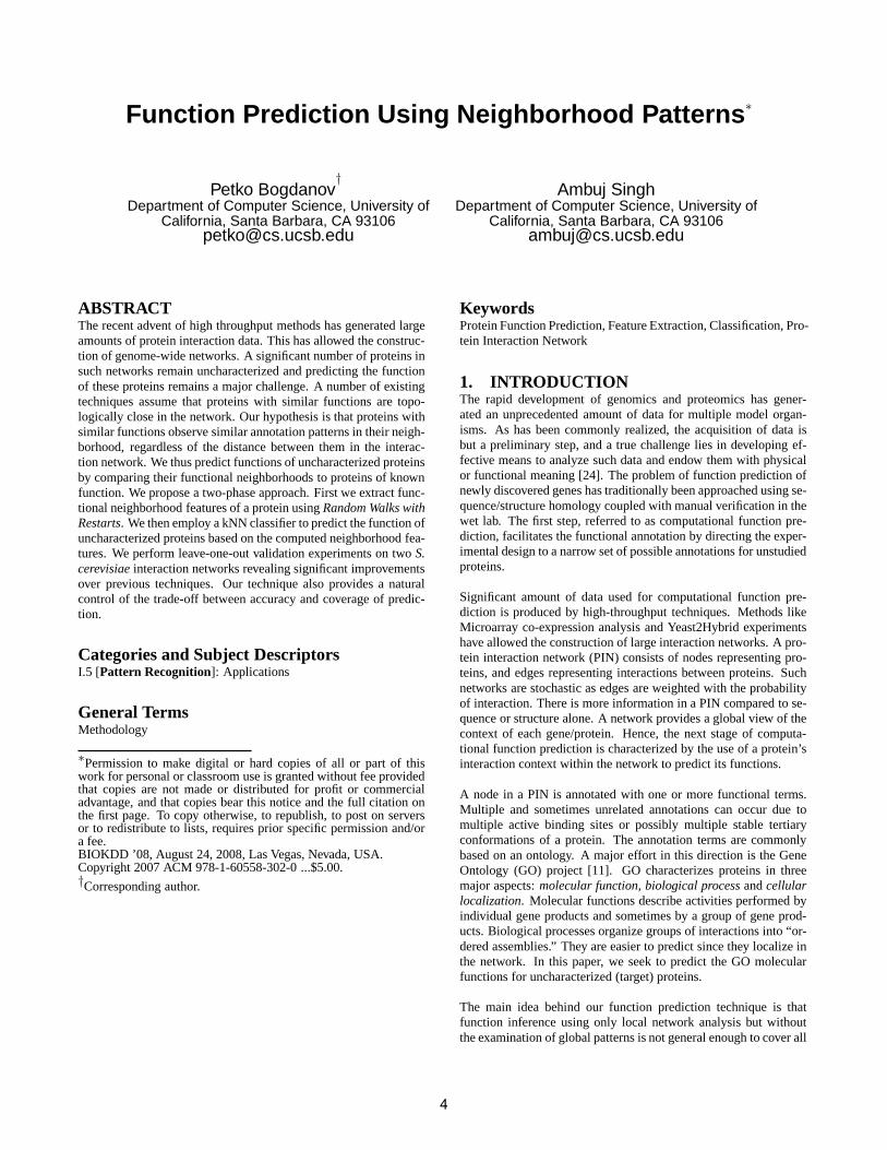
Figure 1: Proteins sharing annotations do not always interactin the Filtered Yeast Interactome (FYI) [12]. Similar functionsare sometimes at large network distances.

We hypothesize that the simultaneous activity of sometimes func-tionally diverse functional agents comprise higher level processesin different regions of the PIN. We refer to this hypothesis asSim-ilar Neighborhood, and to the central idea in all direct methods asFunction Clustering. Our hypothesis is more general, since a cliqueof similar function proteins can be equivalently treated as a set ofnodes that observe the same functional neighborhood. HenceSim-ilar Neighborhoodis a natural generalization ofFunction Cluster-ing. A justification for our approach is provided by Figure 1 whichshows that proteins of similar function may occur at large networkdistances.

3. METHODOur approach divides function prediction into two steps: extrac-tion of neighborhood features, and prediction based on the features.According to ourSimilar Neighborhoodhypothesis, we summarizethe functional network context of a target protein in the neighbor-hood features extraction step. We compute the steady state distri-bution of aRandom Walk with Restarts (RWR)from the protein.The steady state is then transformed into a functional profile. In thesecond step, we employ ak-Nearest-Neighbors (kNN)classifier topredict the function of a target protein based on its functional pro-file. As confirmed by the experimental results, the desired trade-off between accuracy of prediction and coverage of our algorithmcan be controlled byk, the only parameter of the kNN classifica-tion scheme. Such a decoupled approach allows for the possibilitythat other kinds of neighborhood features can be extracted, and thatother kinds of classifiers can be used.

3.1 Extraction of functional profilesThe extraction of features is performed in two steps. First, we char-acterize the neighborhood of a target node with respect to all othernodes in the network. Second, we transform this node-based char-acterization to a function-based one.

We summarize a protein’s neighborhood by computing the steadystate distribution of aRandom Walk with Restarts (RWR). We sim-ulate the trajectory of a random walker that starts from the targetprotein and moves to its neighbors with a probability proportionalto the weight of each connecting edge. We keep the random walkerclose to the original node in order to explore its local neighborhood,by allowing transitions to the original node with a probability ofr,the restart probability [5].

5

The PIN graph is represented by its adjacency matrixMn,n. Eachelementmi,j of M encodes the probability of interaction betweenproteinsi and j. The outgoing edge probabilities of a each pro-tein are normalized, i.e. M is row-normalized. We use the powermethod to compute the steady state vector with respect to eachnode. We term the steady state distribution of nodej as theneigh-borhood profileof proteinj, and denote it asSj , j ∈ [1, n]. Theneighborhood profile is a vector of probabilitiesS

ji , i 6= j, i, j ∈

[1, n]. ComponentSji is proportional to the frequency of visits to

nodei in the RWR fromj. More formally, the power method isdefined as follows:

Sj(t + 1) = (1 − r)MT

Sj(t) + rX. (1)

In the above equation,X is a size-n vector defining the initial stateof the random walk. In the above scenario,X has only one non-zero element corresponding to the target node.Sj(t) is the neigh-borhood profile aftert time steps. The final neighborhood profileis the vectorSj when the process converges. A possible interpre-tation of the neighborhood profile is an affinity vector of the targetnode to all other nodes based solely on the network structure.

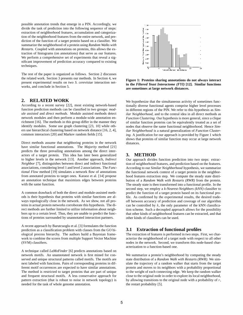
Figure 2: Transformation of the neighborhood profile of node1 into a functional profile. Node 2 is annotated with functionsA and B and node 3 is annotated with functions B and C. Theneighborhood profile of node 1 is computed and transformedusing the annotations on the nodes into a functional profile.

As our goal is to capture the functional context of a protein, thenext step in our feature extraction is the transformation of a neigh-borhood profile into a functional profile. The valueS

ji of nodej

to nodei can be treated as affinity to the annotations ofi. Figure 2illustrates the transformation of a neighborhood profile to a func-tional profile. Assume that RWR performed from node 1 results inthe neighborhood profile(0.7, 0.3), where0.7 corresponds to node2, and0.3 to node 3. Annotations on these two nodes are weightedby the corresponding values, resulting in the vector(0.7, 1.0, 0.3)over functions A, B, and C, respectively. This vector is then nor-malized, resulting into the functional profile(0.35, 0.5, 0.15).

More formally, based on the annotations of a protein, we definean annotation flageia that equals1 if protein i is annotated withfunctiona and0 otherwise. The affinity to each functiona in theneighborhood profile is computed as:

Sj

f (a) =

nX

i=1,i6=j

Sji eia. (2)

VectorSj

f is normalized to yield the functional profile for nodej.

3.2 Function prediction by nearest neighborclassification

The second step in our approach is predicting the annotations ofa given protein based on itsfunctional profile. According to ourSimilar Neighborhoodhypothesis, proteins with similar functionalprofiles are expected to have similar annotations. An intuitive ap-proach in this setting is to annotate a target protein with the annota-tions of the protein with most similar neighborhood. Alternatively,we can explore the topk similar proteins to a target protein andcompute a consensus set of candidate functions.

We formulate function prediction as a multi-class classification prob-lem. Each protein’s profile is an instance (feature vector). Eachinstance can belong to one or more classes as some proteins havemultiple functions. We choose a distance based classification ap-proach to the problem, namely the k-Nearest-Neighbor (kNN) clas-sifier. The classifier uses the L1 distance between the instances andclassifies an instance based on the distributions of classes in itsk

nearest L1 neighbors.

The consensus set of predicted labels is computed using weightedvoting. Annotations of a more similar neighborhood are weightedhigher. The result is a set of scores for each function where a func-tion’s score is computed as follows:

Fja =

kX

i=1

f(d(i, j))eia, (3)

whereeia is an indicator value set to 1 if proteini is annotated witha, d(j, i) is the distance between functional profiles of proteinsi

and j andf(d(i, j)) is a function that transforms the distance toscore. We use a distance-decreasing function of the formf(d) =

1

1+αd, α = 1. It has the desirable property of a finite maximum

at 1 for d = 0, and anti-monotonicity with respect to d. As ourexperiments show, the accuracy did not change significantly whenalternative distance transform functions are used.

It is worth mentioning that since the two steps of our approach arecompletely independent, different approaches can be adopted forfeature extraction and classification. Additionally, it is possible toexploit possible dependencies between the dimensions of the func-tional profile for the purposes of dimensionality reduction.

4. EXPERIMENTAL RESULTS4.1 Interaction and annotation dataWe measure the performance of our method on two yeast proteininteraction networks. As a high confidence interaction network,we use theFiltered Yeast Interactome (FYI)from [12]. This net-work is created by using a collection of interaction data sources,including high throughput yeast two-hybrid, affinity purificationand mass spectrometry,in silico computational predictions of in-teractions, and interaction complexes from MIPS [18]. The net-work contains1379 proteins and1450 interactions.FYI is an un-weighted network, since every edge is added if it exists in morethan two sources [12]. When performing the random walk on thisnetwork, the walker follows a uniformly chosen edge among theoutgoing edges.

The second yeast interaction network is constructed by combin-ing 9 interaction data sources from theBioGRID [1] repository.The method of construction is similar to the ones used in [7, 19,17]. The network consists of4914 proteins and17815 interac-tions among them. TheBioGRIDnetwork contains weighted edgesbased on scoring that takes into account the confidence in each datasource and the magnitude of the interaction.

6

1 2 3 4 5 6 7 80

0.2

0.4

0.6

0.8

1T

P/F

P

Rank

KNN,k=1KNN,k=5KNN,k=10KNN,k=20IndirectFFMajorityRandom

k=1

k=5

k=10k=20

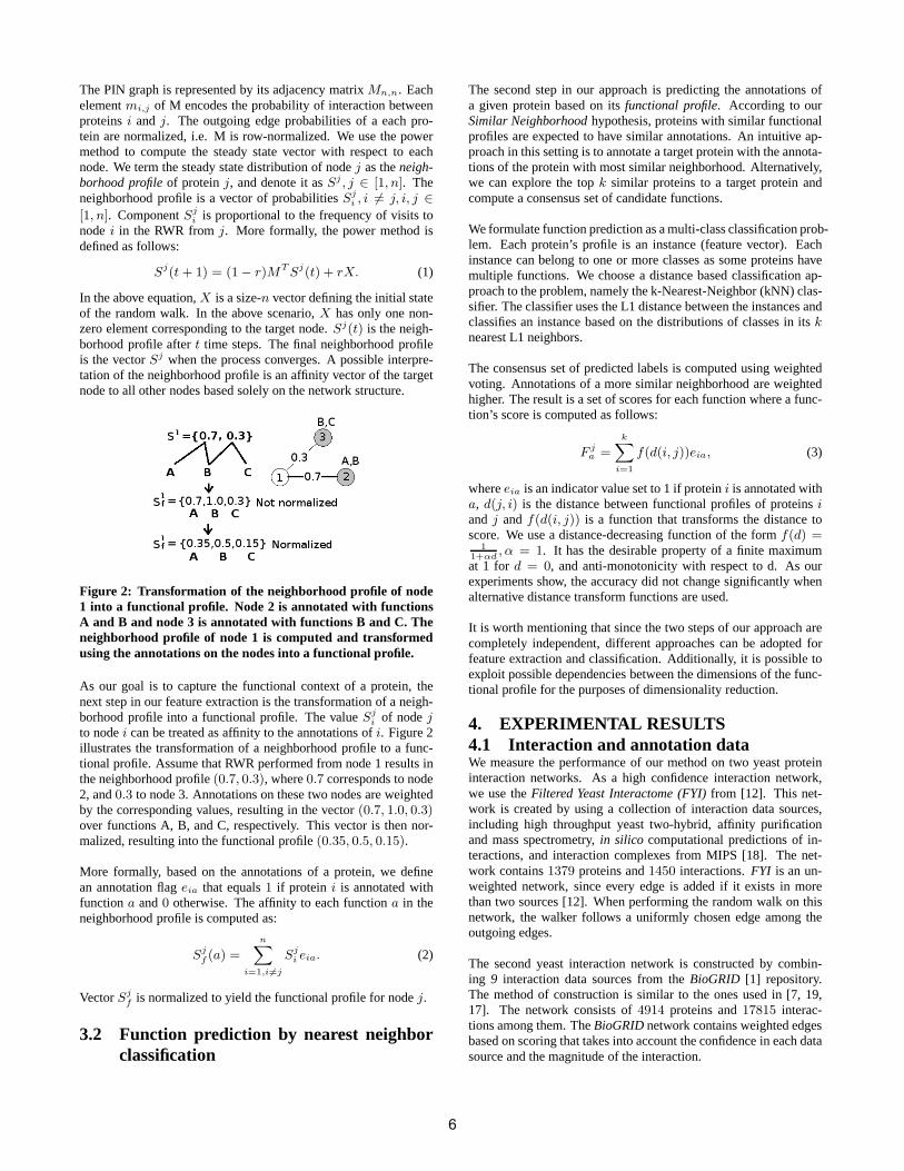
Figure 3: TP/FP ratio for the BioGRID network. All genes arelabeled with exactly one annotation and the value of the fre-quency threshold isT = 30.

The protein GO annotations forS. cerevisiaegene products wereobtained from the Yeast Genome Repository [9].

4.2 Existing techniquesWe compare ourKNN technique toMajority (MAJ) [21], Func-tional Flow (FF) [19] andIndirect Neighbors (Indirect)[7]. Major-ity scores each candidate function based on the number of its occur-rences in the direct interactors. The scores of candidate functionsin edge-weighted networks can be weighted by the probabilities ofthe connecting edges. Functional Flow [19] simulates a discrete-time flow of annotations from all nodes. At every time step, theannotation weight transferred along an edge is proportional to theedge’s weight and the direction of transfer is determined by thedifference of the annotation’s weight in the adjacent nodes. TheIndirect [7] method exploits both indirect and direct function asso-ciations. It computesFunctional Similarityscore based onlevel 1and level 2 interaction partners of a protein. We used the imple-mentation of the method as supplied by the authors, with weightfunction: FSWEIGHT and with minor changes related to the selec-tion of informative functional annotations.

4.3 Experimental setupThe frequency of a functional annotation (class) is the number ofproteins that are annotated with it. We call functions whose fre-quency exceeds a given thresholdT asinformative. An informativeinstance is a protein (represented by its functional profile) anno-tated with at least one informative class. For a givenT , our train-ing instance set contains all informative instances in the network.We exploit all available annotation information and predict func-tions at different levels of specificity. Unlike the approach in [8],we predict informative functions, even if their descendants are alsoinformative.

We compare the accuracy of the techniques by performing leave-one-out validation experiments. We use leave-one-out validationbecause many annotations in the actual network are of relativelylow frequency, and thus limiting the training set. Our classifieris working with actual networks, containing significant number ofuncharacterized proteins and hence this is a realistic measure of theaccuracy. Moreover, since the competing techniques implicitly useall available annoatations, leave-one-out provides a fair comparisonto our method. In this setup, a target protein is held out (i.e. its

1000 2000 3000 4000 5000 6000 7000

500

600

700

800

900

TP

FP

IndirectFFRandomMAJKNN,k=1KNN,k=5KNN,k=10KNN,k=20

(a) BioGRID,T = 30

100 200 300 400 500 600

250

260

270

280

290

300

310

320

330

TP

FP

IndirectMAJKNN,k=1KNN,k=5KNN,k=10KNN,k=20

(b) FYI,T = 20

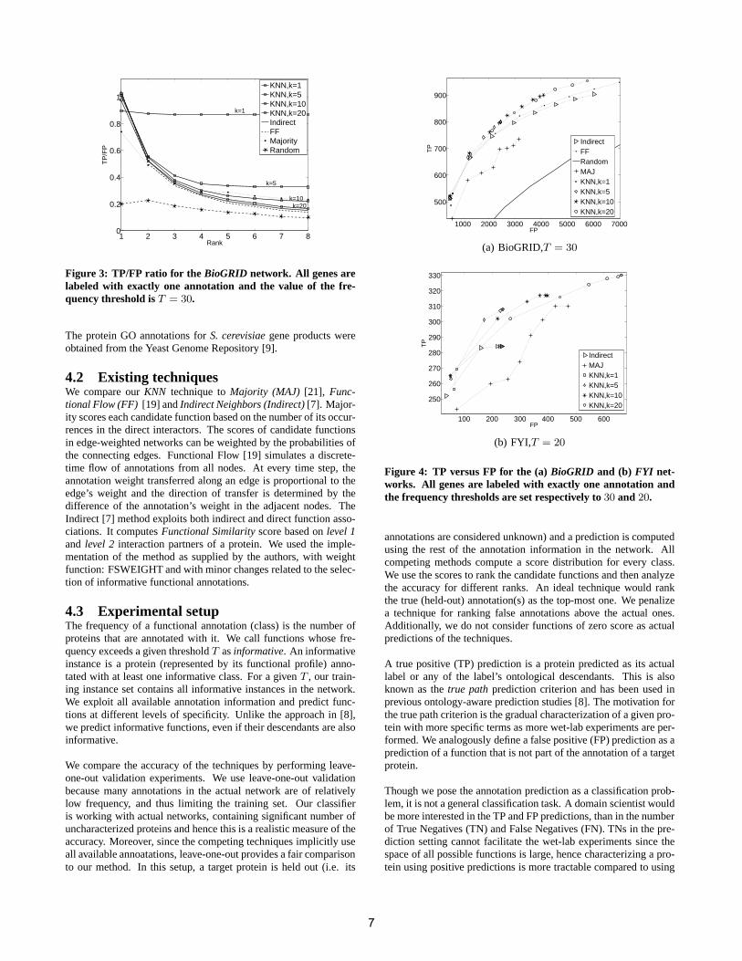
Figure 4: TP versus FP for the (a)BioGRID and (b) FYI net-works. All genes are labeled with exactly one annotation andthe frequency thresholds are set respectively to30 and 20.

annotations are considered unknown) and a prediction is computedusing the rest of the annotation information in the network. Allcompeting methods compute a score distribution for every class.We use the scores to rank the candidate functions and then analyzethe accuracy for different ranks. An ideal technique would rankthe true (held-out) annotation(s) as the top-most one. We penalizea technique for ranking false annotations above the actual ones.Additionally, we do not consider functions of zero score as actualpredictions of the techniques.

A true positive (TP) prediction is a protein predicted as its actuallabel or any of the label’s ontological descendants. This is alsoknown as thetrue pathprediction criterion and has been used inprevious ontology-aware prediction studies [8]. The motivation forthe true path criterion is the gradual characterization of a given pro-tein with more specific terms as more wet-lab experiments are per-formed. We analogously define a false positive (FP) prediction as aprediction of a function that is not part of the annotation of a targetprotein.

Though we pose the annotation prediction as a classification prob-lem, it is not a general classification task. A domain scientist wouldbe more interested in the TP and FP predictions, than in the numberof True Negatives (TN) and False Negatives (FN). TNs in the pre-diction setting cannot facilitate the wet-lab experiments since thespace of all possible functions is large, hence characterizing a pro-tein using positive predictions is more tractable compared to using

7

0 100 200 300 400 500250

260

270

280

290

300

310

320

TP

FP

0.010.10.330.50.8

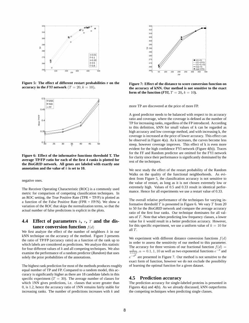
Figure 5: The effect of different restart probabilities r on t heaccuracy in theFYI network (T = 20, k = 10).

20 25 30 35 40 45 500.3

0.35

0.4

0.45

0.5

Mea

n T

P/F

P

T

kNNINDFF

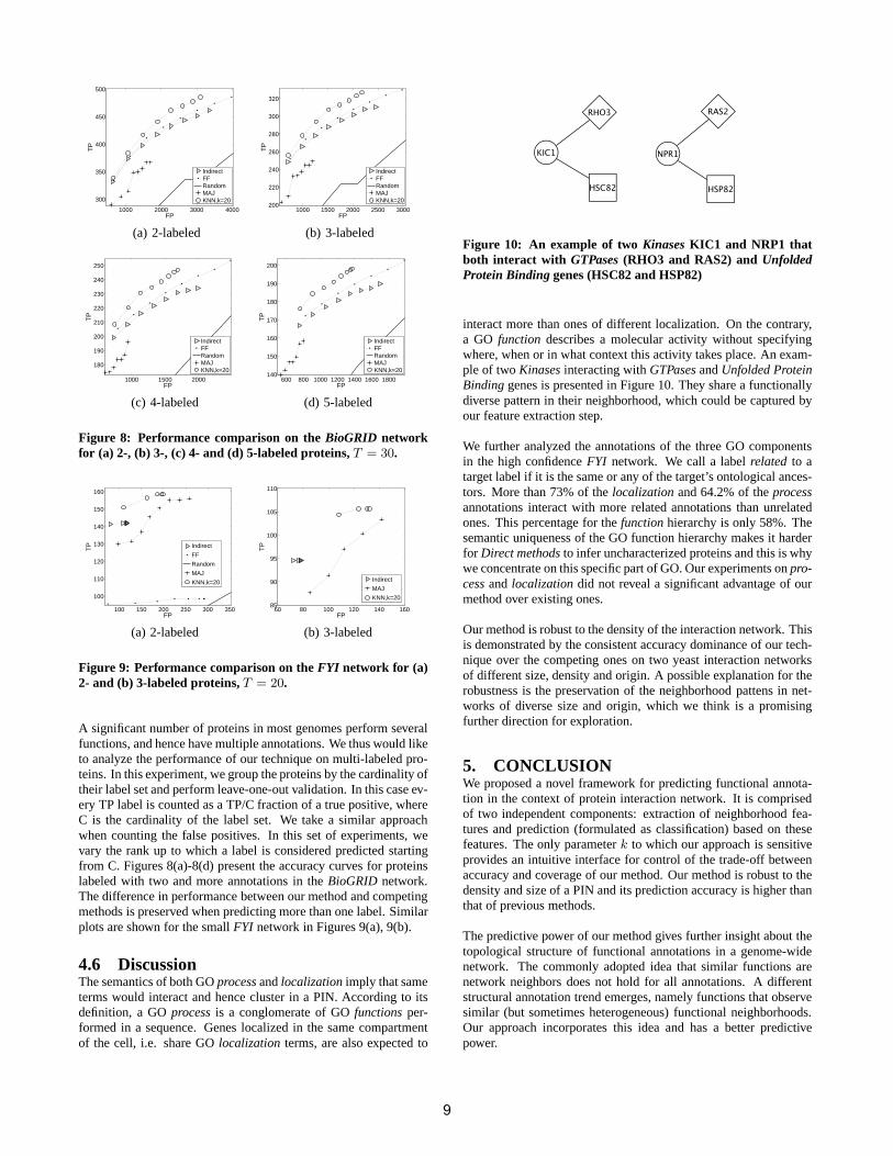
Figure 6: Effect of the informative functions threshold T. Theaverage TP/FP ratio for each of the first 4 ranks is plotted forthe BioGRID network. All genes are labeled with exactly oneannotation and the value ofk is set to 10.

negative ones.

The Receiver Operating Characteristic (ROC) is a commonly usedmetric for comparison of competing classification techniques. Inan ROC setting, the True Positive Rate (TPR = TP/P) is plotted asa function of the False Positive Rate (FPR = FP/N). We show avariation of the ROC that skips the normalization terms, so that theactual number of false predictions is explicit in the plots.

4.4 Effect of parametersk, r, T and the dis-tance conversion functionf(d)

We first analyze the effect of the number of neighborsk in ourkNN technique on the accuracy of the method. Figure 3 presentsthe ratio of TP/FP (accuracy ratio) as a function of the rank up towhich labels are considered as predictions. We analyze this statisticfor four different values ofk and all competing techniques. We alsoexamine the performance of a random predictor (Random) that usessolely the prior probabilities of the annotations.

The highest rank prediction for most of the methods produces roughlyequal number of TP and FP. Compared to a random model, this ac-curacy is significantly higher as there are 18 candidate labels in thisspecific experiment (T = 30). The average number of classes forwhich 1NN gives predictions, i.e. classes that score greater than0, is 1.2, hence the accuracy ratio of 1NN remains fairly stable forincreasing ranks. The number of predictions increases withk and

0 50 100 150 200 250 300 350 400260

265

270

275

280

285

290

295

300

305

310

315

320

TP

FP

1/(1+D)1/(1+10*D)1/(1+0.1*D)exp(−D)exp(−D*D)

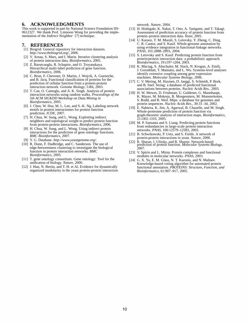
Figure 7: Effect of the distance to score conversion functiononthe accuracy of kNN. Our method is not sensitive to the exactform of the function (FYI, T = 20, k = 10).

more TP are discovered at the price of more FP.

A good predictor needs to be balanced with respect to its accuracyratio and coverage, where the coverage is defined as the number ofTP for increasing ranks, regardless of the FP introduced. Accordingto this definition, kNN for small values of k can be regarded ashigh accuracy and low coverage method, and with increasing k, thecoverage is increased at the price of lower accuracy. This effect canbe observed in Figure 4(a). As k increases, the curves become lesssteep, however coverage improves. This effect of k is even moreevident for the high confidence FYI network (Figure 4(b)). Tracesfor the FF and Random predictor are omitted for the FYI networkfor clarity since their performance is significantly dominated by therest of the techniques.

We next study the effect of the restart probability of the RandomWalks on the quality of the functional neighborhoods. As evi-dent from Figure 5, the classification accuracy is not sensitive tothe value of restart, as long as it is not chosen extremely low orextremely high. Values of 0.5 and 0.33 result in identical perfor-mance. Hence for all experiments we use a restart value of 0.33.

The overall relative performance of the techniques for varying in-formative thresholdT is presented in Figure 6. We varyT from 20to 50 for theBioGRIDnetwork and compare the average accuracyratio of the first four ranks. Our technique dominates for all val-ues ofT . Note that when predicting low frequency classes, a lowervalue fork would result in a better prediction accuracy. However,for this specific experiment, we use a uniform value ofk = 10 forall T .

We experiment with different distance conversion functionsf(d)in order to assess the sensitivity of our method to this parameter.The accuracy for three versions of our fractional functionf(d) =

1

1+αd, α = 0.1, 1, 10 as well as two exponential functionse−d and

e−d2

are presented in Figure 7. Our method is not sensitive to theexact form of function, however we do not exclude the possibilityof learning the optimal function for a given dataset.

4.5 Prediction accuracyThe prediction accuracy for single-labeled proteins is presented inFigures 4(a) and 4(b). As we already discussed, kNN outperformsthe competing techniques when predicting single classes.

8

1000 2000 3000 4000

300

350

400

450

500T

P

FP

IndirectFFRandomMAJKNN,k=20

(a) 2-labeled

1000 1500 2000 2500 3000200

220

240

260

280

300

320

TP

FP

IndirectFFRandomMAJKNN,k=20

(b) 3-labeled

1000 1500 2000

180

190

200

210

220

230

240

250

TP

FP

IndirectFFRandomMAJKNN,k=20

(c) 4-labeled

600 800 1000 1200 1400 1600 1800140

150

160

170

180

190

200T

P

FP

IndirectFFRandomMAJKNN,k=20

(d) 5-labeled

Figure 8: Performance comparison on theBioGRID networkfor (a) 2-, (b) 3-, (c) 4- and (d) 5-labeled proteins,T = 30.

100 150 200 250 300 350

100

110

120

130

140

150

160

TP

FP

Indirect

FF

Random

MAJ

KNN,k=20

(a) 2-labeled

60 80 100 120 140 16085

90

95

100

105

110

TP

FP

Indirect

MAJ

KNN,k=20

(b) 3-labeled

Figure 9: Performance comparison on theFYI network for (a)2- and (b) 3-labeled proteins,T = 20.

A significant number of proteins in most genomes perform severalfunctions, and hence have multiple annotations. We thus would liketo analyze the performance of our technique on multi-labeled pro-teins. In this experiment, we group the proteins by the cardinality oftheir label set and perform leave-one-out validation. In this case ev-ery TP label is counted as a TP/C fraction of a true positive, whereC is the cardinality of the label set. We take a similar approachwhen counting the false positives. In this set of experiments, wevary the rank up to which a label is considered predicted startingfrom C. Figures 8(a)-8(d) present the accuracy curves for proteinslabeled with two and more annotations in theBioGRID network.The difference in performance between our method and competingmethods is preserved when predicting more than one label. Similarplots are shown for the smallFYI network in Figures 9(a), 9(b).

4.6 DiscussionThe semantics of both GOprocessandlocalizationimply that sameterms would interact and hence cluster in a PIN. According to itsdefinition, a GOprocessis a conglomerate of GOfunctionsper-formed in a sequence. Genes localized in the same compartmentof the cell, i.e. share GOlocalization terms, are also expected to

Figure 10: An example of two Kinases KIC1 and NRP1 thatboth interact with GTPases (RHO3 and RAS2) andUnfoldedProtein Binding genes (HSC82 and HSP82)

interact more than ones of different localization. On the contrary,a GO function describes a molecular activity without specifyingwhere, when or in what context this activity takes place. An exam-ple of twoKinasesinteracting withGTPasesandUnfolded ProteinBindinggenes is presented in Figure 10. They share a functionallydiverse pattern in their neighborhood, which could be captured byour feature extraction step.

We further analyzed the annotations of the three GO componentsin the high confidenceFYI network. We call a labelrelated to atarget label if it is the same or any of the target’s ontological ances-tors. More than 73% of thelocalizationand 64.2% of theprocessannotations interact with more related annotations than unrelatedones. This percentage for thefunctionhierarchy is only 58%. Thesemantic uniqueness of the GO function hierarchy makes it harderfor Direct methodsto infer uncharacterized proteins and this is whywe concentrate on this specific part of GO. Our experiments onpro-cessand localizationdid not reveal a significant advantage of ourmethod over existing ones.

Our method is robust to the density of the interaction network. Thisis demonstrated by the consistent accuracy dominance of our tech-nique over the competing ones on two yeast interaction networksof different size, density and origin. A possible explanation for therobustness is the preservation of the neighborhood pattens in net-works of diverse size and origin, which we think is a promisingfurther direction for exploration.

5. CONCLUSIONWe proposed a novel framework for predicting functional annota-tion in the context of protein interaction network. It is comprisedof two independent components: extraction of neighborhood fea-tures and prediction (formulated as classification) based on thesefeatures. The only parameterk to which our approach is sensitiveprovides an intuitive interface for control of the trade-off betweenaccuracy and coverage of our method. Our method is robust to thedensity and size of a PIN and its prediction accuracy is higher thanthat of previous methods.

The predictive power of our method gives further insight about thetopological structure of functional annotations in a genome-widenetwork. The commonly adopted idea that similar functions arenetwork neighbors does not hold for all annotations. A differentstructural annotation trend emerges, namely functions that observesimilar (but sometimes heterogeneous) functional neighborhoods.Our approach incorporates this idea and has a better predictivepower.

9

6. ACKNOWLEDGMENTSThis work is supported in part by National Science Foundation IIS-0612327. We thank Prof. Limsoon Wong for providing the imple-mentation of theIndirect Neighbor [7] technique.

7. REFERENCES[1] Biogrid: General repository for interaction datasets.

http://www.thebiogrid.org/, 2006.[2] V. Arnau, S. Mars, and I. Marin. Iterative clustering analysis

of protein interaction data.Bioinformatics, 2005.[3] Z. Barutcuoglu, R. Schapire, and O. Troyanskaya.

Hierarchical multi-label prediction of gene function.Bioinformatics, 2006.

[4] C. Brun, F. Chevenet, D. Martin, J. Wojcik, A. Guenoche,and B. Jacq. Functional classification of proteins for theprediction of cellular function from a protein-proteininteraction network.Genome Biology, 5:R6, 2003.

[5] T. Can, O. Camoglu, and A. K. Singh. Analysis of proteininteraction networks using random walks.Proceedings of the5th ACM SIGKDD Workshop on Data Mining inBioinformatics, 2005.

[6] J. Chen, W. Hsu, M. L. Lee, and S.-K. Ng. Labeling networkmotifs in protein interactomes for protein functionprediction.ICDE, 2007.

[7] H. Chua, W. Sung, and L. Wong. Exploiting indirectneighbors and topological weight to predict protein functionfrom protein-protein interactions.Bioinformatics, 2006.

[8] H. Chua, W. Sung, and L. Wong. Using indirect proteininteractions for the prediction of gene ontology functions.BMC Bioinformatics, 2007.

[9] Y. G. Database.http://www.yeastgenome.org/.[10] R. Dunn, F. Dudbridge, and C. Sanderson. The use of

edge-betweenness clustering to investigate the biologicalfunction in protein interaction networks.BMCBioinformatics, 2005.

[11] T. gene ontology consortium. Gene ontology: Tool for theunification of biology.Nature, 2000.

[12] J. Han, N. Bertin, and T. H. et Al. Evidence for dynamicallyorganized modularity in the yeast protein-protein interaction

network.Nature, 2004.[13] H. Hishigaki, K. Nakai, T. Ono, A. Tanigami, and T. Takagi.

Assessment of prediction accuracy of protein function fromprotein–protein interaction data.Yeast, 2001.

[14] U. Karaoz, T. M. Murali, S. Letovsky, Y. Zheng, C. Ding,C. R. Cantor, and S. Kasif. Whole-genome annotation byusing evidence integration in functional-linkage networks.PNAS, 101:2888–2893, 2004.

[15] S. Letovsky and S. Kasif. Predicting protein function fromprotein/protein interaction data: a probabilistic approach.Bioinformatics, 19:i197–i204, 2003.

[16] K. Maciag, S. Altschuler, M. Slack, N. Krogan, A. Emili,J. Greenblatt, T. Maniatis, and L. Wu. Systems-level analysesidentify extensive coupling among gene expressionmachines.Molecular Systems Biology, 2006.

[17] C. V. Mering, M. Huynen, D. Jaeggi, S. Schmidt, P. Bork,and B. Snel. String: a database of predicted functionalassociations between proteins.Nucleic Acids Res., 2003.

[18] H. W. Mewes, D. Frishman, U. Guldener, G. Mannhaupt,K. Mayer, M. Mokrejs, B. Morgenstern, M. Munsterkotter,S. Rudd, and B. Weil. Mips: a database for genomes andprotein sequences.Nucleic Acids Res., 30:31–34, 2002.

[19] E. Nabieva, K. Jim, A. Agarwal, B. Chazelle, and M. Singh.Whole-proteome prediction of protein function viagraph-theoretic analysis of interaction maps.Bioinformatics,21:i302–i310, 2005.

[20] M. P. Samanta and S. Liang. Predicting protein functionsfrom redundancies in large-scale protein interactionnetworks.PNAS, 100:12579–12583, 2003.

[21] B. Schwikowski, P. Uetz, and S. Fields. A network ofprotein-protein interactions in yeast.Nature, 2000.

[22] R. Sharan, I. Ulitsky, and R. Shamir. Network-basedprediction of protein function.Molecular Systems Biology,2007.

[23] V. Spirin and L. Mirny. Protein complexes and functionalmodules in molecular networks.PNAS, 2003.

[24] G. X. Yu, E. M. Glass, N. T. Karonis, and N. Maltsev.Knowledge-based voting algorithm for automated proteinfunctional annotation.PROTEINS: Structure, Function, andBioinformatics, 61:907–917, 2005.

10

Statistical modeling of medical indexing processes forbiomedical knowledge information discovery from text

Markus BundschusInstitute for Computer Science

University of MunichOettingenstr. 67

80538 Munich, Germanybundschu@dbs.ifi.lmu.de

Mathaeus DejoriIntegrated Data Systems Dep.Siemens Corporate Research

755 College Road EastPrinceton, NJ 08540, USA

mathaeus.dejori@siemens.com

Shipeng YuCAD & Knowledge SolutionsSiemens Medical Solutions51 Valley Stream ParkwayMalvern, PA 19355, USA

shipeng.yu@siemens.com

Volker TrespInformation &

Communications, IC4Siemens CT

Otto-Hahn-Ring 681739 Munich, Germany

volker.tresp@siemens.com

Hans-Peter KriegelInstitute for Computer Science

University of MunichOettingenstr. 67

80538 Munich, Germanykriegel@dbs.ifi.lmu.de

ABSTRACTThe overwhelming amount of published literature in thebiomedical domain and the growing number of collabora-tions across scientific disciplines results in an increasing top-ical complexity of research articles. This represents an im-mense challenge for efficient biomedical knowledge discov-ery from text. We present a new graphical model, the so-called Topic-Concept Model, which extends the basic La-tent Dirichlet Allocation framework and reflects the gener-ative process of indexing a PubMed abstract with termino-logical concepts from an ontology. The generative modelcaptures the latent topic structure of documents by learn-ing the statistical dependencies between words, topics andMeSH (Medical Subject Headings) concepts. A number ofimportant tasks for biomedical knowledge discovery can besolved with the here introduced model. We provide resultsfor the extraction of the hidden topic-concept structure froma large medical text collection, the identification of the mostlikely topics given a specific MeSH concept, and the extrac-tion of statistical relationships between MeSH concepts andwords. Moreover, we apply the introduced generative modelto a challenging multi-label classification task. A benchmarkwith several classification methods on two independent datasets proves our method to be competitive.

KeywordsDocument Modeling, topic modeling, multi-label classifica-tion, ontologies

Permission to make digital or hard copies of all or part of this work forpersonal or classroom use is granted without fee provided that copies arenot made or distributed for profit or commercial advantage and that copiesbear this notice and the full citation on the first page. To copy otherwise, torepublish, to post on servers or to redistribute to lists, requires prior specificpermission and/or a fee.BIOKDD ’08 Las Vegas, NV, USACopyright 2008 ACM 978-1-60558-302-0 ...$5.00.

1. INTRODUCTIONIn the last decade, powerful new biomedical research tools

and methods have been developed, resulting in an unprece-dented increase of biomedical data and literature. High-throughput experiments, such as DNA microarrays or pro-tein arrays, produce large quantities of high-quality data,leading to an explosion of scientific articles published in thisfield. Thus, automated extraction of useful information fromlarge document collections has become an increasingly im-portant research area [12, 11]. To ensure an efficient ac-cess to this steadily increasing source of bibliographic infor-mation, it is required to efficiently index incoming articles,i. e. to label unstructured free text with a structured ma-chine readable annotation. Articles selected for inclusion inPubMed1, for example, are indexed with concepts from theMedical Subject Headings2 (MeSH) thesaurus to facilitatelater retrieval. This additional meta information provides arich source of knowledge, which can be exploited for biomed-ical knowledge discovery and data mining tasks and this isthe focus of this work.

Recently, powerful techniques such as Probabilistic LatentSemantic Analysis (PLSA) [15] or Latent Dirichlet Alloca-tion (LDA) [7] have been proposed for automated extractionof useful information from large document collections. Ap-plications include automatic topic extraction, query answer-ing, document summarization, and trend analysis. Gener-ative statistical models such as the above mentioned ones,have been proven effective in addressing these problems. Ingeneral, the following advantages of topic models are high-lighted in the context of document modeling: First, topicscan be extracted in a complete unsupervised fashion, requir-ing no initial labeling of the topics. Second, the resultingrepresentation of topics for a document collection is inter-pretable and last but not least, each document is usuallyexpressed by a mixture of topics, thus capturing the topiccombinations that arise in documents [15, 7, 14]. In the

1http://www.ncbi.nlm.nih.gov/pubmed/2http://www.nlm.nih.gov/mesh/

11

biomedical domain, the classical LDA model has been ap-plied to the task of finding life span related genes from theCaenorhabditis Genetic Center Bibliography [5] and to thetask of identifying biological concepts from a protein-relatedcorpus [33]. Depending on the addressed generative process,the LDA framework has been extended e. g. to model the de-pendencies between authors, topics and documents [30] orthe dependencies between author and recipients [20]. Fur-ther approaches include the modeling of images and theircorresponding captions [6] as well as the modeling of depen-dencies between topics and named entities [25].

In this paper, we introduce another extension of the LDAframework, the so-called Topic-Concept (TC) model, to re-semble the generative process of creating an indexed PubMedabstract. The approach simultaneously models the way howthe document is generated as well as the way how the docu-ment is subsequently indexed with MeSH concepts (see fig-ure 1 for a comparison with the classical LDA approach).We refer to MeSH as a terminological ontology, where rela-tions are partially described as subtype-supertype relationsand where the concepts are described by concept labels orsynonyms [2].

By modeling the indexing process of PubMed abstracts,we can answer a range of important queries for knowledgediscovery about the content of biomedical text collections.With such a model, we can provide a bird’s eye view ofbiomedical topics discussed in a large document collectionassociated with prominent MeSH concepts (i. e. uncoveringthe hidden topic-concept structure in a biomedical text col-lection). In contrast to the classical LDA, this results ina richer representation of topics, since topics are not solelyrepresented by their most likely words. Instead, topics in theTC model are, in addition to the words, associated with theirmost likely MeSH terms (see section 3.2.1). Furthermore, wecan identify several types of statistical relationships betweendifferent classes of document entities (i. e. words, MeSH con-cepts and topics). We provide results for identifying statis-tical relationships between concepts and words based on thetopics (see section 3.2.2). Another interesting use case weconsider, is the estimation of the most likely topics givena MeSH concept. This results in a fast overview over thetopics in which a specific MeSH term is most likely to beinvolved (see section 3.2.2). Last but not least, we can usethe TC model for multi-label classification. To validate thepredictive power of the here presented model, we apply ourgenerative method to a challenging multi-label classificationproblem with 108 classes. A benchmark on two independentcorpora against (1) a multi-label naive Bayes classifier, (2) amethod currently used by the National Library of Medicine(NLM) and (3) a state-of-the-art multi-label support vectormachine (SVM) shows encouraging results.

The remainder of the paper is organized as follows: InSection 2 we describe the extension of the classical LDA to-wards the TC model. Section 3.1 describes the experimentalsetup. Afterwards results are presented and a concludingdiscussion is given.

2. METHODSIn the following we will describe two generative mod-

els, the first simulating the process of document generationalone and the second simulating both the process of docu-ment generation and the process of document indexing. Let

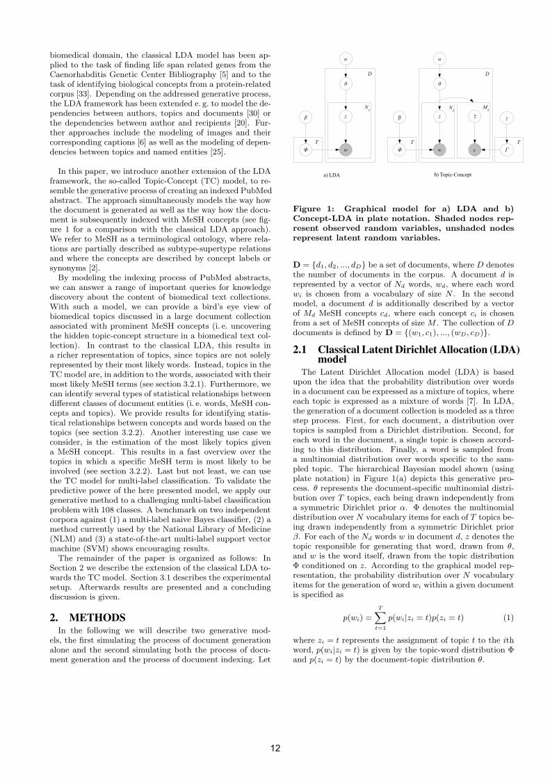
Figure 1: Graphical model for a) LDA and b)Concept-LDA in plate notation. Shaded nodes rep-resent observed random variables, unshaded nodesrepresent latent random variables.

D = {d1, d2, ..., dD} be a set of documents, where D denotesthe number of documents in the corpus. A document d isrepresented by a vector of Nd words, wd, where each wordwi is chosen from a vocabulary of size N . In the secondmodel, a document d is additionally described by a vectorof Md MeSH concepts cd, where each concept ci is chosenfrom a set of MeSH concepts of size M . The collection of Ddocuments is defined by D = {(w1, c1), ..., (wD, cD)}.

2.1 Classical Latent Dirichlet Allocation (LDA)model

The Latent Dirichlet Allocation model (LDA) is basedupon the idea that the probability distribution over wordsin a document can be expressed as a mixture of topics, whereeach topic is expressed as a mixture of words [7]. In LDA,the generation of a document collection is modeled as a threestep process. First, for each document, a distribution overtopics is sampled from a Dirichlet distribution. Second, foreach word in the document, a single topic is chosen accord-ing to this distribution. Finally, a word is sampled froma multinomial distribution over words specific to the sam-pled topic. The hierarchical Bayesian model shown (usingplate notation) in Figure 1(a) depicts this generative pro-cess. θ represents the document-specific multinomial distri-bution over T topics, each being drawn independently froma symmetric Dirichlet prior α. Φ denotes the multinomialdistribution over N vocabulary items for each of T topics be-ing drawn independently from a symmetric Dirichlet priorβ. For each of the Nd words w in document d, z denotes thetopic responsible for generating that word, drawn from θ,and w is the word itself, drawn from the topic distributionΦ conditioned on z. According to the graphical model rep-resentation, the probability distribution over N vocabularyitems for the generation of word wi within a given documentis specified as

p(wi) =

T∑t=1

p(wi|zi = t)p(zi = t) (1)

where zi = t represents the assignment of topic t to the ithword, p(wi|zi = t) is given by the topic-word distribution Φand p(zi = t) by the document-topic distribution θ.

12

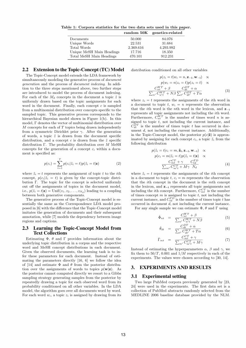
Table 1: Corpora statistics for the two data sets used in this paper.

random 50K genetics-related

Documents 50.000 84.076Unique Words 22.531 31.684Total Words 2.369.616 4.293.992Unique MeSH Main Headings 17.716 18.350Total MeSH Main Headings 470.101 912.231

2.2 Extension to the Topic-Concept (TC) ModelThe Topic-Concept model extends the LDA framework by

simultaneously modeling the generative process of documentgeneration and the process of document indexing. In addi-tion to the three steps mentioned above, two further stepsare introduced to model the process of document indexing.For each of the Md concepts in the document a topic z isuniformly drawn based on the topic assignments for eachword in the document. Finally, each concept c is sampledfrom a multinomial distribution over concepts specific to thesampled topic. This generative process corresponds to thehierarchical Bayesian model shown in Figure 1(b). In thismodel, Γ denotes the vector of multinomial distribution overM concepts for each of T topics being drawn independentlyfrom a symmetric Dirichlet prior γ. After the generationof words, a topic z is drawn from the document specificdistribution, and a concept c is drawn from the z specificdistribution Γ. The probability distribution over M MeSHconcepts for the generation of a concept ci within a docu-ment is specified as:

p(ci) =

T∑t=1

p(ci|zi = t)p(zi = t|z) (2)

where zi = t represents the assignment of topic t to the ithconcept, p(ci|zi = t) is given by the concept-topic distri-bution Γ. The topic for the concept is selected uniformlyout off the assignments of topics in the document model,i.e., p(zi = t|z) = Unif(z1, z2, . . . , zNd) leading to a couplingbetween both generative components.

The generative process of the Topic-Concept model is es-sentially the same as the Correspondence LDA model pro-posed in [6] with the difference that the Topic-Concept modelimitates the generation of documents and their subsequentannotation, while [7] models the dependency between imageregions and captions.

2.3 Learning the Topic-Concept Model fromText Collections

Estimating Φ, θ and Γ provides information about theunderlying topic distribution in a corpus and the respectiveword and MeSH concept distributions in each document.Given the observed documents, the learning task is to in-fer these parameters for each document. Instead of esti-mating the parameters directly [16, 6] we follow the ideaof [14] and estimate Φ and θ from the posterior distribu-tion over the assignments of words to topics p(w|z). Asthe posterior cannot computed directly we resort to a Gibbssampling strategy generating samples from the posterior byrepeatedly drawing a topic for each observed word from itsprobability conditioned on all other variables. In the LDAmodel, the algorithm goes over all documents word by word.For each word wi, a topic zi is assigned by drawing from its

distribution conditioned on all other variables

p(zi = t|wi = n, z−i,w−i) ∝p(wi = n|zi = t)p(zi = t) ∝

CWTnt + β∑

n′ CWTn′t +Nβ

CDTdt + α∑

t′ CDTdt′ + Tα

(3)

where zi = t represents the assignments of the ith word ina document to topic t, wi = n represents the observationthat the ith word is the nth word in the lexicon, and z−i

represents all topic assignments not including the ith word.Furthermore, CWT

nt is the number of times word n is as-signed to topic t, not including the current instance, andCDT

dt is the number of times topic t has occurred in doc-ument d, not including the current instance. Additionally,in the Topic-Concept model, the posterior p(c|z) is approx-imated by assigning for each concept ci, a topic zi from thefollowing distribution

p(zi = t|ci = m, zi, z−i,w−i) ∝p(ci = m|zi = t)p(zi = t|z) ∝

CCTmt + γ∑

m′ CCTm′t +Mγ

CTDtd

Nd(4)

where zi = t represents the assignments of the ith conceptin a document to topic t, ci = m represents the observationthat the ith concept in the document is the mth conceptin the lexicon, and z−i represents all topic assignments notincluding the ith concept. Furthermore, CCT

mt is the numberof times concept m is assigned to topic t, not including thecurrent instance, and CTD

td is the number of times topic t hasoccurred in document d, not including the current instance.

For any single sample we can estimate Φ, θ and Γ using

Φnt =CWT

nt + β∑n′ CWT

n′t +Nβ(5)

θdt =CDT

dt + α∑t′ C

WTdt′ + Tα

(6)

Γmt =CCT

mt + γ∑m′ CCT

m′t +Mγ(7)

Instead of estimating the hyperparameters α, β and γ, wefix them to 50/T , 0.001 and 1/M respectively in each of theexperiments. The values were chosen according to [30, 14].

3. EXPERIMENTS AND RESULTS

3.1 Experimental settingTwo large PubMed corpora previously generated by [23,

24] were used in the experiments. The first data set is acollection of PubMed abstracts randomly selected from theMEDLINE 2006 baseline database provided by the NLM.

13

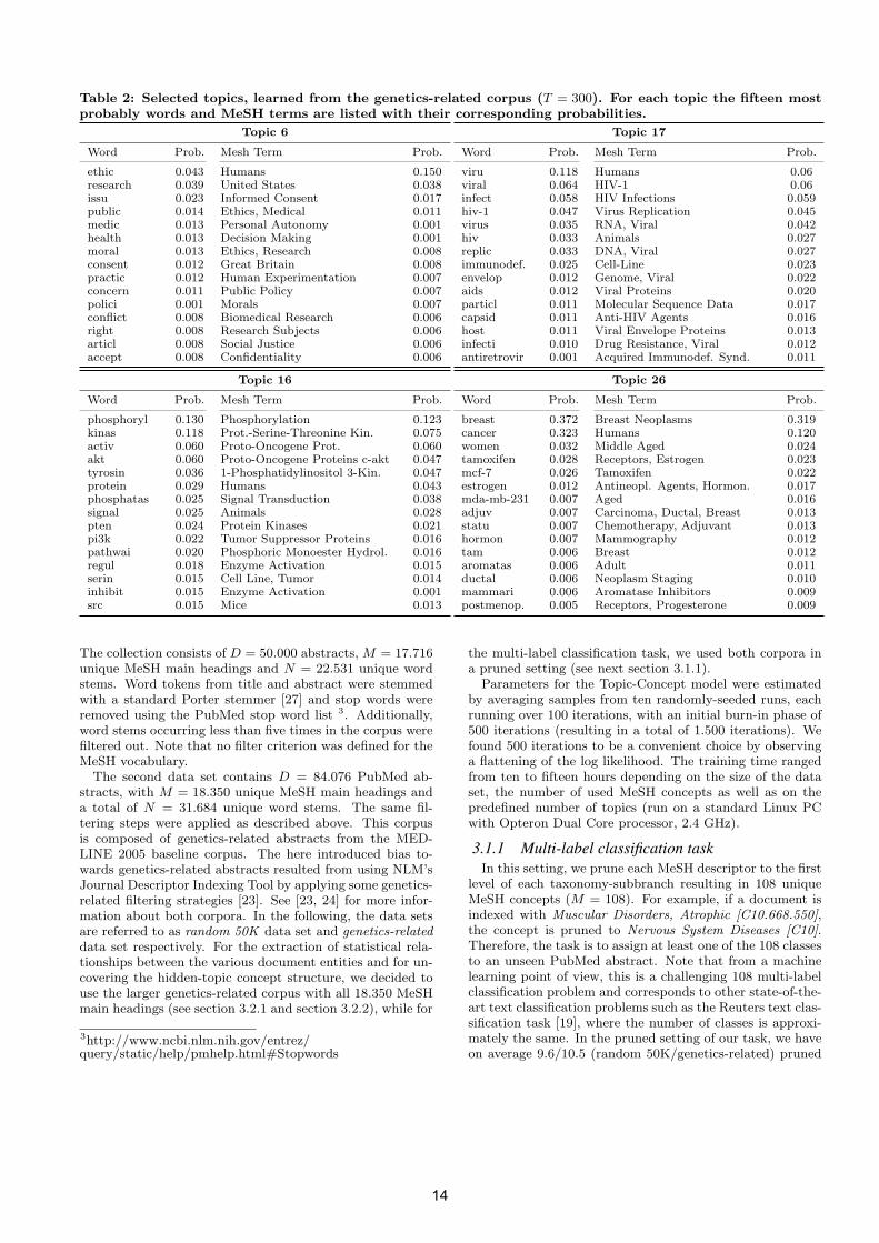
Table 2: Selected topics, learned from the genetics-related corpus (T = 300). For each topic the fifteen mostprobably words and MeSH terms are listed with their corresponding probabilities.

Topic 6

Word Prob. Mesh Term Prob.

ethic 0.043 Humans 0.150research 0.039 United States 0.038issu 0.023 Informed Consent 0.017public 0.014 Ethics, Medical 0.011medic 0.013 Personal Autonomy 0.001health 0.013 Decision Making 0.001moral 0.013 Ethics, Research 0.008consent 0.012 Great Britain 0.008practic 0.012 Human Experimentation 0.007concern 0.011 Public Policy 0.007polici 0.001 Morals 0.007conflict 0.008 Biomedical Research 0.006right 0.008 Research Subjects 0.006articl 0.008 Social Justice 0.006accept 0.008 Confidentiality 0.006

Topic 17

Word Prob. Mesh Term Prob.

viru 0.118 Humans 0.06viral 0.064 HIV-1 0.06infect 0.058 HIV Infections 0.059hiv-1 0.047 Virus Replication 0.045virus 0.035 RNA, Viral 0.042hiv 0.033 Animals 0.027replic 0.033 DNA, Viral 0.027immunodef. 0.025 Cell-Line 0.023envelop 0.012 Genome, Viral 0.022aids 0.012 Viral Proteins 0.020particl 0.011 Molecular Sequence Data 0.017capsid 0.011 Anti-HIV Agents 0.016host 0.011 Viral Envelope Proteins 0.013infecti 0.010 Drug Resistance, Viral 0.012antiretrovir 0.001 Acquired Immunodef. Synd. 0.011

Topic 16

Word Prob. Mesh Term Prob.

phosphoryl 0.130 Phosphorylation 0.123kinas 0.118 Prot.-Serine-Threonine Kin. 0.075activ 0.060 Proto-Oncogene Prot. 0.060akt 0.060 Proto-Oncogene Proteins c-akt 0.047tyrosin 0.036 1-Phosphatidylinositol 3-Kin. 0.047protein 0.029 Humans 0.043phosphatas 0.025 Signal Transduction 0.038signal 0.025 Animals 0.028pten 0.024 Protein Kinases 0.021pi3k 0.022 Tumor Suppressor Proteins 0.016pathwai 0.020 Phosphoric Monoester Hydrol. 0.016regul 0.018 Enzyme Activation 0.015serin 0.015 Cell Line, Tumor 0.014inhibit 0.015 Enzyme Activation 0.001src 0.015 Mice 0.013

Topic 26

Word Prob. Mesh Term Prob.

breast 0.372 Breast Neoplasms 0.319cancer 0.323 Humans 0.120women 0.032 Middle Aged 0.024tamoxifen 0.028 Receptors, Estrogen 0.023mcf-7 0.026 Tamoxifen 0.022estrogen 0.012 Antineopl. Agents, Hormon. 0.017mda-mb-231 0.007 Aged 0.016adjuv 0.007 Carcinoma, Ductal, Breast 0.013statu 0.007 Chemotherapy, Adjuvant 0.013hormon 0.007 Mammography 0.012tam 0.006 Breast 0.012aromatas 0.006 Adult 0.011ductal 0.006 Neoplasm Staging 0.010mammari 0.006 Aromatase Inhibitors 0.009postmenop. 0.005 Receptors, Progesterone 0.009

The collection consists of D = 50.000 abstracts, M = 17.716unique MeSH main headings and N = 22.531 unique wordstems. Word tokens from title and abstract were stemmedwith a standard Porter stemmer [27] and stop words wereremoved using the PubMed stop word list 3. Additionally,word stems occurring less than five times in the corpus werefiltered out. Note that no filter criterion was defined for theMeSH vocabulary.

The second data set contains D = 84.076 PubMed ab-stracts, with M = 18.350 unique MeSH main headings anda total of N = 31.684 unique word stems. The same fil-tering steps were applied as described above. This corpusis composed of genetics-related abstracts from the MED-LINE 2005 baseline corpus. The here introduced bias to-wards genetics-related abstracts resulted from using NLM’sJournal Descriptor Indexing Tool by applying some genetics-related filtering strategies [23]. See [23, 24] for more infor-mation about both corpora. In the following, the data setsare referred to as random 50K data set and genetics-relateddata set respectively. For the extraction of statistical rela-tionships between the various document entities and for un-covering the hidden-topic concept structure, we decided touse the larger genetics-related corpus with all 18.350 MeSHmain headings (see section 3.2.1 and section 3.2.2), while for

3http://www.ncbi.nlm.nih.gov/entrez/query/static/help/pmhelp.html#Stopwords

the multi-label classification task, we used both corpora ina pruned setting (see next section 3.1.1).

Parameters for the Topic-Concept model were estimatedby averaging samples from ten randomly-seeded runs, eachrunning over 100 iterations, with an initial burn-in phase of500 iterations (resulting in a total of 1.500 iterations). Wefound 500 iterations to be a convenient choice by observinga flattening of the log likelihood. The training time rangedfrom ten to fifteen hours depending on the size of the dataset, the number of used MeSH concepts as well as on thepredefined number of topics (run on a standard Linux PCwith Opteron Dual Core processor, 2.4 GHz).

3.1.1 Multi-label classification taskIn this setting, we prune each MeSH descriptor to the first

level of each taxonomy-subbranch resulting in 108 uniqueMeSH concepts (M = 108). For example, if a document isindexed with Muscular Disorders, Atrophic [C10.668.550],the concept is pruned to Nervous System Diseases [C10].Therefore, the task is to assign at least one of the 108 classesto an unseen PubMed abstract. Note that from a machinelearning point of view, this is a challenging 108 multi-labelclassification problem and corresponds to other state-of-the-art text classification problems such as the Reuters text clas-sification task [19], where the number of classes is approxi-mately the same. In the pruned setting of our task, we haveon average 9.6/10.5 (random 50K/genetics-related) pruned

14

Table 3: Selected MeSH concepts from the Disease and the Drug & Chemicals subbranch with the 20 mostprobable word stems estimated based on a topic-concept model learned from the genetics-related corpus(T = 300). The font size of each word stem encodes its probability given the corresponding MeSH concept.The number in brackets is euqal to the number of times, the MeSH terms occurs in the corpus

Diseases

Myelodysplastic Syndromes (208)

acut aml bcr-abl blast chronic cml flt3hematolog imatinib leukaemia leukem

leukemia lymphoblast marrow

mds myelodysplast myeloid patient relapssyndrom

Pulmonary Embolism (39)

activ associ case clinic diagnos

diagnosi diagnost factor incid men

mortal patient platelet preval

protein rate risk studi women year

Drugs & Chemicals

Erythropoietin (85)abnorm anaemia anemia caus cell defect

defici disord epo erythrocyt erythroiderythropoietin g6pd hemoglobin increas model

normal patient sever studi

Paclitaxel (309)

advanc agent anticanc cancer

chemotherapi cisplatin combin cytotox

drug effect median paclitaxel

patient phase regimen respons sensit

surviv toxic treatment

MeSH labels per document. Parameter estimation remainsthe same as mentioned in the previous paragraph.

In particular, we are interested in evaluating the classi-fication task in a user-centered or semi-automatic scenario,where we want to recommend a set of classes for a specificdocument (e. g. a human indexer gets recommendations ofMeSH terms for a document). Thus, we decided to followthe evaluation of [13] and average the effectiveness of theclassifiers over documents rather than over categories. Inaddition, we weight recall over precision and use the F2-macro measure, because it reflects that human indexers willaccept some inappropriate recommendations as long as themajor fraction of recommended index terms will be correct[13].

3.2 Results

3.2.1 Uncovering the hidden topic-concept structure

Table 2 illustrates several different topics (out of 300)from the genetics-related corpus, obtained from a partic-ular Gibbs sampler run after the 1.500th iteration. Eachtable shows the fifteen most likely word stems assigned to aspecific topic and its corresponding most likely MeSH mainheadings. To show the descriptive power of our learnedmodel, we chose four topics describing different aspects ofbiomedical research. Topic 6 is ethics-related, topic 16 is re-lated to a special biochemical process, namely signal trans-duction, and the last two topics represent aspects of specificdisease classes. Topic 26 represents a topic centered aroundbreast cancer, while topic 17 refers to HIV. The model in-cludes several other topics related to specific diseases, bio-chemical processes, organs and other aspects of biomedicalresearch like e. g. Magnetic Resonance Spectroscopy. Recallthat the here investigated corpus is biased towards genetics-related topics, thus, some topics can describe quite specificaspects of genetics research. More generic topics in the cor-pus are related to terms, common to almost all biomedical

research areas including terminology, describing experimen-tal setups or methods. In general, the extracted topics are,of course, dependent on the corpus seed. The full list of top-ics with corresponding word and MeSH distributions is avail-able at www.dbs.ifi.lmu.de/~bundschu/TCmodel_supplementary/TC_structure.txt.

It can be seen that the word stems already provide an intu-itive description of specific aspects. Furthermore, the topicsgain more descriptive power by their associated MeSH con-cepts, providing an accurate description in structured from.Note that the standard topic models are only able to rep-resent topics with the single word descriptions. In contrast,the TC model provides a richer representation of topics byadditionally linking topics to concepts from a terminologicalontology. We found that the topics obtained from differentGibbs sampling runs were relatively stable. A variability interms of ranking of the words and MeSH terms in the topicscan be observed, but overall the topics match very closely.For studies about topic stability in aspect models, pleaserefer to [29].

3.2.2 Extraction of statistical relationshipsBesides uncovering the hidden topic-concept structure,

we apply the model to derive statistical relations betweenMeSH concepts and word stems, thus bridging the gap be-tween natural free text and the structured semantic anno-tation. The derived relations could be e. g. used for im-proving word sense disambiguation [18]. In Table 3, fourMeSH concepts from the Disease and the Drug & Chemi-cals subbranch and their twenty most probable word stemsare shown. For each MeSH concept, the distribution overwords is graphically represented by varying the font size foreach word stem with respect to the probability. Given a con-cept c, the conditional probability for each word is estimatedby p(w|c) ∝

∑t p(w|t)p(t|c), which is computed from the

learned model parameters. The word distributions describethe corresponding MeSH concept in an intuitive way, cap-turing the topical diversity of certain MeSH concepts. Note

15

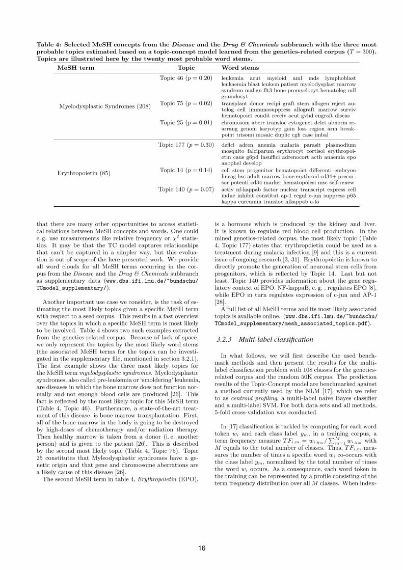
Table 4: Selected MeSH concepts from the Disease and the Drug & Chemicals subbranch with the three mostprobable topics estimated based on a topic-concept model learned from the genetics-related corpus (T = 300).Topics are illustrated here by the twenty most probable word stems.

MeSH term Topic Word stems

Myelodysplastic Syndromes (208)

Topic 46 (p = 0.20) leukemia acut myeloid aml mds lymphoblastleukaemia blast leukem patient myelodysplast marrowsyndrom malign flt3 bone promyelocyt hematolog mllgranulocyt

Topic 75 (p = 0.02) transplant donor recipi graft stem allogen reject au-tolog cell immunosuppress allograft marrow survivhematopoiet condit receiv acut gvhd engraft diseas

Topic 25 (p = 0.01) chromosom aberr transloc cytogenet delet abnorm re-arrang genom karyotyp gain loss region arm break-point trisomi mosaic duplic cgh case imbal

Erythropoietin (85)

Topic 177 (p = 0.30) defici adren anemia malaria parasit plasmodiummosquito falciparum erythrocyt cortisol erythropoi-etin caus g6pd insuffici adrenocort acth anaemia epoanophel develop

Topic 14 (p = 0.14) cell stem progenitor hematopoiet differenti embryonlineag hsc adult marrow bone erythroid cd34+ precur-sor potenti cd34 marker hematopoiesi msc self-renew

Topic 140 (p = 0.07) activ nf-kappab factor nuclear transcript express cellinduc inhibit constitut ap-1 regul c-jun suppress p65kappa curcumin transloc nfkappab c-fo

that there are many other opportunities to access statisti-cal relations between MeSH concepts and words. One coulde. g. use measurements like relative frequency or χ2 statis-tics. It may be that the TC model captures relationshipsthat can’t be captured in a simpler way, but this evalua-tion is out of scope of the here presented work. We provideall word clouds for all MeSH terms occurring in the cor-pus from the Disease and the Drug & Chemicals subbranchas supplementary data (www.dbs.ifi.lmu.de/~bundschu/TCmodel_supplementary/).

Another important use case we consider, is the task of es-timating the most likely topics given a specific MeSH termwith respect to a seed corpus. This results in a fast overviewover the topics in which a specific MeSH term is most likelyto be involved. Table 4 shows two such examples extractedfrom the genetics-related corpus. Because of lack of space,we only represent the topics by the most likely word stems(the associated MeSH terms for the topics can be investi-gated in the supplementary file, mentioned in section 3.2.1).The first example shows the three most likely topics forthe MeSH term myelodysplastic syndromes. Myelodysplasticsyndromes, also called pre-leukemia or ‘smoldering’ leukemia,are diseases in which the bone marrow does not function nor-mally and not enough blood cells are produced [26]. Thisfact is reflected by the most likely topic for this MeSH term(Table 4, Topic 46). Furthermore, a state-of-the-art treat-ment of this disease, is bone marrow transplantation. First,all of the bone marrow in the body is going to be destroyedby high-doses of chemotherapy and/or radiation therapy.Then healthy marrow is taken from a donor (i. e. anotherperson) and is given to the patient [26]. This is describedby the second most likely topic (Table 4, Topic 75). Topic25 constitutes that Myleodysplastic syndromes have a ge-netic origin and that gene and chromosome aberrations area likely cause of this disease [26].

The second MeSH term in table 4, Erythropoietin (EPO),

is a hormone which is produced by the kidney and liver.It is known to regulate red blood cell production. In themined genetics-related corpus, the most likely topic (Table4, Topic 177) states that erythropoietin could be used as atreatment during malaria infection [9] and this is a currentissue of ongoing research [3, 31]. Erythropoietin is known todirectly promote the generation of neuronal stem cells fromprogenitors, which is reflected by Topic 14. Last but notleast, Topic 140 provides information about the gene regu-latory context of EPO. NF-kappaB, e. g. , regulates EPO [8],while EPO in turn regulates expression of c-jun and AP-1[28].

A full list of all MeSH terms and its most likely associatedtopics is available online. (www.dbs.ifi.lmu.de/~bundschu/TCmodel_supplementary/mesh_associated_topics.pdf).

3.2.3 Multi-label classification

In what follows, we will first describe the used bench-mark methods and then present the results for the multi-label classification problem with 108 classes for the genetics-related corpus and the random 50K corpus. The predictionresults of the Topic-Concept model are benchmarked againsta method currently used by the NLM [17], which we referto as centroid profiling, a multi-label naive Bayes classifierand a multi-label SVM. For both data sets and all methods,5-fold cross-validation was conducted.

In [17] classification is tackled by computing for each wordtoken wi and each class label ym, in a training corpus, aterm frequency measure TFi,m = wi,ym/

∑Mm=1 wi,ym with

M equals to the total number of classes. Thus, TFi,m mea-sures the number of times a specific word wi co-occurs withthe class label ym, normalized by the total number of timesthe word wi occurs. As a consequence, each word token inthe training can be represented by a profile consisting of theterm frequency distribution over all M classes. When index-

16

0 5 10 15 20 25 300.1

0.2

0.3

0.4

0.5

0.6

0.7

0.8

Number of recommended MeSH terms

F2−

mac

ro

F2−macro comparison

Centroid ProfilingSVM, TfSVM, Tf−IdfTC model, T=600

0 5 10 15 20 25 300.1

0.2

0.3

0.4

0.5

0.6

0.7

0.8

0.9

1

Number of recommended MeSH terms

Rec

all

Recall comparison

Centroid ProfilingSVM, TfSVM, Tf−IdfTC model, T=600

0 5 10 15 20 25 300.2

0.3

0.4

0.5

0.6

0.7

0.8

0.9

1

Number of recommended MeSH terms

Pre

cisi

on

Precision comparison

Centroid ProfilingSVM, TfSVM, Tf−IdfTC model, T=600

(a) random 50K corpus

0 5 10 15 20 25 300.1

0.2

0.3

0.4

0.5

0.6

0.7

0.8

Number of recommended MeSH terms

F2−

mac

ro

F2−macro comparison

Centroid ProfilingSVM, TfSVM, Tf−IdfTC model, T=600

0 5 10 15 20 25 300

0.1

0.2

0.3

0.4

0.5

0.6

0.7

0.8

0.9

1

Number of recommended MeSH terms

Rec

all

Recall comparison

Centroid ProfilingSVM, TfSVM, Tf−IdfTC model, T=600

0 5 10 15 20 25 30

0.4

0.5

0.6

0.7

0.8

0.9

1

Number of recommended MeSH terms

Pre

cisi

on

Precision comparison

Centroid ProfilingSVM, TfSVM, Tf−IdfTC model, T=600

(b) genetics-related corpus

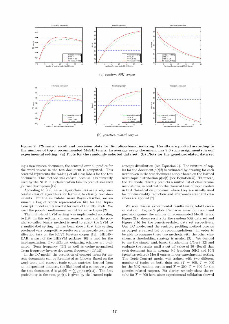
Figure 2: F2-macro, recall and precision plots for discipline-based indexing. Results are plotted according tothe number of top n recommended MeSH terms. In average every document has 9.6 such assignments in ourexperimental setting. (a) Plots for the randomly selected data set. (b) Plots for the genetics-related data set

ing a new unseen document, the centroid over all profiles forthe word tokens in the test document is computed. Thiscentroid represents the ranking of all class labels for the testdocument. This method was chosen, because it is currentlyused by the NLM in a classification task to predict so-calledjournal descriptors [17].

According to [22], naive Bayes classifiers are a very suc-cessful class of algorithms for learning to classify text doc-uments. For the multi-label naive Bayes classifier, we as-sumed a bag of words representation like for the Topic-Concept model and trained it for each of the 108 labels. Weused the popular multinomial model for naive Bayes [21].

The multi-label SVM setting was implemented accordingto [19]. In this setting, a linear kernel is used and the pop-ular so-called binary method is used to adapt the SVM toa multi-label setting. It has been shown that this settingproduced very competitive results on a large-scale text clas-sification task on the RCV1 Reuters corpus [19]. LIBLIN-EAR, a part of the LIBSVM package [10] is used for theimplementation. Two different weighting schemes are eval-uated: Term frequency (Tf) as well as cosine-normalizedTerm frequency-inverse document frequency (Tf-Idf).

In the TC-model, the prediction of concept terms for un-seen documents can be formulated as follows: Based on theword-topic and concept-topic count matrices learned froman independent data set, the likelihood of a concept c giventhe test document d is p(c|d) =

∑t p(c|t)p(t|d). The first

probability in the sum, p(c|t), is given by the learned topic-

concept distribution (see Equation 7). The mixture of top-ics for the document p(t|d) is estimated by drawing for eachword token in the test document a topic based on the learnedword-topic distribution p(w|t) (see Equation 5). Therefore,the TC model directly predicts a ranked list of class recom-mendations, in contrast to the classical task of topic modelsin text classification problems, where they are usually usedfor dimensionality reduction and afterwards standard clas-sifiers are applied [7].

We now discuss experimental results using 5-fold cross-validation. Figure 2 plots F2-macro measure, recall andprecision against the number of recommended MeSH terms.Figure 2(a) shows results for the random 50K data set andFigure 2(b) for the genetics-related data set respectively.Our TC model and the centroid profiling method provideas output a ranked list of recommendations. In order tobe able to compare these two methods with the other clas-sifiers, a thresholding strategy is needed [32]. We decidedto use the simple rank-based thresholding (Rcut) [32] andevaluate the results until a cut-off value of 30 (Recall thateach document has in average 9.6 (random 50K) and 10.5(genetics-related) MeSH entries in our experimental setting.The Topic-Concept model was trained with two differentnumber of topics on both data sets (T = 300, T = 600for the 50K random corpus and T = 300, T = 600 for thegenetics-related corpus). For clarity, we only show the re-sults for T = 600 here, since experimental validation showed

17

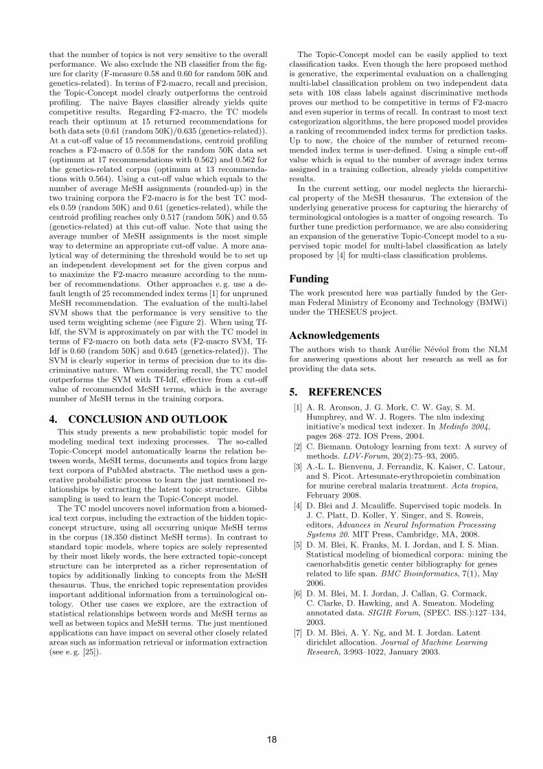
that the number of topics is not very sensitive to the overallperformance. We also exclude the NB classifier from the fig-ure for clarity (F-measure 0.58 and 0.60 for random 50K andgenetics-related). In terms of F2-macro, recall and precision,the Topic-Concept model clearly outperforms the centroidprofiling. The naive Bayes classifier already yields quitecompetitive results. Regarding F2-macro, the TC modelsreach their optimum at 15 returned recommendations forboth data sets (0.61 (random 50K)/0.635 (genetics-related)).At a cut-off value of 15 recommendations, centroid profilingreaches a F2-macro of 0.558 for the random 50K data set(optimum at 17 recommendations with 0.562) and 0.562 forthe genetics-related corpus (optimum at 13 recommenda-tions with 0.564). Using a cut-off value which equals to thenumber of average MeSH assignments (rounded-up) in thetwo training corpora the F2-macro is for the best TC mod-els 0.59 (random 50K) and 0.61 (genetics-related), while thecentroid profiling reaches only 0.517 (random 50K) and 0.55(genetics-related) at this cut-off value. Note that using theaverage number of MeSH assignments is the most simpleway to determine an appropriate cut-off value. A more ana-lytical way of determining the threshold would be to set upan independent development set for the given corpus andto maximize the F2-macro measure according to the num-ber of recommendations. Other approaches e. g. use a de-fault length of 25 recommended index terms [1] for unprunedMeSH recommendation. The evaluation of the multi-labelSVM shows that the performance is very sensitive to theused term weighting scheme (see Figure 2). When using Tf-Idf, the SVM is approximately on par with the TC model interms of F2-macro on both data sets (F2-macro SVM, Tf-Idf is 0.60 (random 50K) and 0.645 (genetics-related)). TheSVM is clearly superior in terms of precision due to its dis-criminative nature. When considering recall, the TC modeloutperforms the SVM with Tf-Idf, effective from a cut-offvalue of recommended MeSH terms, which is the averagenumber of MeSH terms in the training corpora.

4. CONCLUSION AND OUTLOOKThis study presents a new probabilistic topic model for

modeling medical text indexing processes. The so-calledTopic-Concept model automatically learns the relation be-tween words, MeSH terms, documents and topics from largetext corpora of PubMed abstracts. The method uses a gen-erative probabilistic process to learn the just mentioned re-lationships by extracting the latent topic structure. Gibbssampling is used to learn the Topic-Concept model.

The TC model uncovers novel information from a biomed-ical text corpus, including the extraction of the hidden topic-concept structure, using all occurring unique MeSH termsin the corpus (18.350 distinct MeSH terms). In contrast tostandard topic models, where topics are solely representedby their most likely words, the here extracted topic-conceptstructure can be interpreted as a richer representation oftopics by additionally linking to concepts from the MeSHthesaurus. Thus, the enriched topic representation providesimportant additional information from a terminological on-tology. Other use cases we explore, are the extraction ofstatistical relationships between words and MeSH terms aswell as between topics and MeSH terms. The just mentionedapplications can have impact on several other closely relatedareas such as information retrieval or information extraction(see e. g. [25]).

The Topic-Concept model can be easily applied to textclassification tasks. Even though the here proposed methodis generative, the experimental evaluation on a challengingmulti-label classification problem on two independent datasets with 108 class labels against discriminative methodsproves our method to be competitive in terms of F2-macroand even superior in terms of recall. In contrast to most textcategorization algorithms, the here proposed model providesa ranking of recommended index terms for prediction tasks.Up to now, the choice of the number of returned recom-mended index terms is user-defined. Using a simple cut-offvalue which is equal to the number of average index termsassigned in a training collection, already yields competitiveresults.

In the current setting, our model neglects the hierarchi-cal property of the MeSH thesaurus. The extension of theunderlying generative process for capturing the hierarchy ofterminological ontologies is a matter of ongoing research. Tofurther tune prediction performance, we are also consideringan expansion of the generative Topic-Concept model to a su-pervised topic model for multi-label classification as latelyproposed by [4] for multi-class classification problems.

FundingThe work presented here was partially funded by the Ger-man Federal Ministry of Economy and Technology (BMWi)under the THESEUS project.

AcknowledgementsThe authors wish to thank Aurelie Neveol from the NLMfor answering questions about her research as well as forproviding the data sets.

5. REFERENCES[1] A. R. Aronson, J. G. Mork, C. W. Gay, S. M.

Humphrey, and W. J. Rogers. The nlm indexinginitiative’s medical text indexer. In Medinfo 2004,pages 268–272. IOS Press, 2004.

[2] C. Biemann. Ontology learning from text: A survey ofmethods. LDV-Forum, 20(2):75–93, 2005.

[3] A.-L. L. Bienvenu, J. Ferrandiz, K. Kaiser, C. Latour,and S. Picot. Artesunate-erythropoietin combinationfor murine cerebral malaria treatment. Acta tropica,February 2008.

[4] D. Blei and J. Mcauliffe. Supervised topic models. InJ. C. Platt, D. Koller, Y. Singer, and S. Roweis,editors, Advances in Neural Information ProcessingSystems 20. MIT Press, Cambridge, MA, 2008.

[5] D. M. Blei, K. Franks, M. I. Jordan, and I. S. Mian.Statistical modeling of biomedical corpora: mining thecaenorhabditis genetic center bibliography for genesrelated to life span. BMC Bioinformatics, 7(1), May2006.

[6] D. M. Blei, M. I. Jordan, J. Callan, G. Cormack,C. Clarke, D. Hawking, and A. Smeaton. Modelingannotated data. SIGIR Forum, (SPEC. ISS.):127–134,2003.

[7] D. M. Blei, A. Y. Ng, and M. I. Jordan. Latentdirichlet allocation. Journal of Machine LearningResearch, 3:993–1022, January 2003.

18

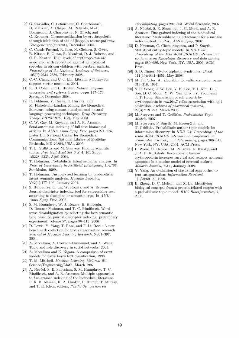
[8] G. Carvalho, C. Lefaucheur, C. Cherbonnier,D. Metivier, A. Chapel, M. Pallardy, M.-F.Bourgeade, B. Charpentier, F. Hirsch, andG. Kroemer. Chemosensitization by erythropoietinthrough inhibition of the nf-[kappa]b rescue pathway.Oncogene, aop(current), December 2004.

[9] C. Casals-Pascual, R. Idro, N. Gicheru, S. Gwer,B. Kitsao, E. Gitau, R. Mwakesi, D. J. Roberts, andC. R. Newton. High levels of erythropoietin areassociated with protection against neurologicalsequelae in african children with cerebral malaria.Proceedings of the National Academy of Sciences,105(7):2634–2639, February 2008.

[10] C.-C. Chang and C.-J. Lin. Libsvm: a library forsupport vector machines, 2001.

[11] K. B. Cohen and L. Hunter. Natural languageprocessing and systems biology, pages 147–174.Springer, December 2004.

[12] R. Feldman, Y. Regev, E. Hurvitz, andM. Finkelstein-Landau. Mining the biomedicalliterature using semantic analysis and naturallanguage processing techniques. Drug DiscoveryToday: BIOSILICO, 1(2), May 2003.

[13] C. W. Gay, M. Kayaalp, and A. R. Aronson.Semi-automatic indexing of full text biomedicalarticles. In AMIA Annu Symp Proc, pages 271–275,Lister Hill National Center for BiomedicalCommunications, National Library of Medicine,Bethesda, MD 20894, USA., 2005.

[14] T. L. Griffiths and M. Steyvers. Finding scientifictopics. Proc Natl Acad Sci U S A, 101 Suppl1:5228–5235, April 2004.

[15] T. Hofmann. Probabilistic latent semantic analysis. InProc. of Uncertainty in Artificial Intelligence, UAI’99,Stockholm, 1999.

[16] T. Hofmann. Unsupervised learning by probabilisticlatent semantic analysis. Machine Learning,V42(1):177–196, January 2001.

[17] S. Humphrey, C. Lu, W. Rogers, and A. Browne.Journal descriptor indexing tool for categorizing textaccording to discipline or semantic type. In AMIAAnnu Symp Proc, 2006.

[18] S. M. Humphrey, W. J. Rogers, H. Kilicoglu,D. Demner-Fushman, and T. C. Rindflesch. Wordsense disambiguation by selecting the best semantictype based on journal descriptor indexing: preliminaryexperiment. volume 57, pages 96–113, 2006.

[19] D. Lewis, Y. Yang, T. Rose, and F. Li. Rcv1: A newbenchmark collection for text categorization research.Journal of Machine Learning Research, 5:361–397,2004.

[20] A. Mccallum, A. Corrada-Emmanuel, and X. Wang.Topic and role discovery in social networks. 2005.

[21] A. Mccallum and K. Nigam. A comparison of eventmodels for naive bayes text classification, 1998.

[22] T. M. Mitchell. Machine Learning. McGraw-HillScience/Engineering/Math, March 1997.

[23] A. Neveol, S. E. Shooshan, S. M. Humphrey, T. C.Rindflesch, and A. R. Aronson. Multiple approachesto fine-grained indexing of the biomedical literature.In R. B. Altman, K. A. Dunker, L. Hunter, T. Murray,and T. E. Klein, editors, Pacific Symposium on

Biocomputing, pages 292–303. World Scientific, 2007.

[24] A. Neveol, S. E. Shooshan, J. G. Mork, and A. R.Aronson. Fine-grained indexing of the biomedicalliterature: Mesh subheading attachment for a medlineindexing tool. In Proc. AMIA Symp, 2007.

[25] D. Newman, C. Chemudugunta, and P. Smyth.Statistical entity-topic models. In KDD ’06:Proceedings of the 12th ACM SIGKDD internationalconference on Knowledge discovery and data mining,pages 680–686, New York, NY, USA, 2006. ACMPress.

[26] S. D. Nimer. Myelodysplastic syndromes. Blood,111(10):4841–4851, May 2008.

[27] M. F. Porter. An algorithm for suffix stripping. pages313–316, 1997.

[28] S. R. Seong, J. W. Lee, Y. K. Lee, T. I. Kim, D. J.Son, D. C. Moon, Y. W. Yun, d. o. . Y. Yoon, andJ. T. Hong. Stimulation of cell growth byerythropoietin in raw264.7 cells: association with ap-1activation. Archives of pharmacal research,29(3):218–223, March 2006.

[29] M. Steyvers and T. Griffiths. Probabilistic TopicModels. 2007.

[30] M. Steyvers, P. Smyth, M. Rosen-Zvi, andT. Griffiths. Probabilistic author-topic models forinformation discovery. In KDD ’04: Proceedings of thetenth ACM SIGKDD international conference onKnowledge discovery and data mining, pages 306–315,New York, NY, USA, 2004. ACM Press.

[31] L. Wiese, C. Hempel, M. Penkowa, N. Kirkby, andJ. A. L. Kurtzhals. Recombinant humanerythropoietin increases survival and reduces neuronalapoptosis in a murine model of cerebral malaria.Malaria Journal, 7:3+, January 2008.

[32] Y. Yang. An evaluation of statistical approaches totext categorization. Information Retrieval,1(1/2):69–90, 1999.

[33] B. Zheng, D. C. Mclean, and X. Lu. Identifyingbiological concepts from a protein-related corpus witha probabilistic topic model. BMC Bioinformatics, 7,2006.

19

Information Theoretic Methods for Detecting Multiple Loci Associated with Complex Diseases

ABSTRACT Gene-gene interactions play important roles in the etiology of complex multi-factorial diseases. With the advancements in genotyping technology, large genetic association studies based on hundreds of thousands of single-nucleotide polymorphisms are a popular option for the study of complex diseases. Association studies using locus by locus analyses till remains the primary method although the study of gene-gene interactions has become more common using regression based methods. However, regression based methods are computationally heavy and model complexity increases rapidly with the increase in number of loci and also with the number of possible allelic states at each locus. Information theoretic approaches offer many potent capabilities and advantages for the analyses of gene-gene interactions. In this paper, we develop and explore the effectiveness of two information theoretic metrics in identifying gene-gene interactions using extensive simulations on four different gene-gene interaction models. We propose a forward selection algorithm using the metrics and evaluate its performance using the rheumatoid arthritis dataset from Genetic Analysis Workshop-15. We demonstrate that our metrics are capable of analyzing a diverse range of epidemiological data sets containing evidences for gene-gene interactions.

Keywords Gene-gene interaction, information theory, entropy, complex diseases.

1. INTRODUCTION

Complex interactions involving a number of genes and multiple single nucleotide polymorphisms (SNP) and environmental factors are known to be associated with the risk of developing diseases such as cancer, autoimmune disease and cardiovascular disease. Advances in high throughput genotyping methods and the completion of human genome project have made generating large

scale dense genetic maps of the human genome for epidemiological studies feasible [1, 2]. The successful identification of critical gene-gene and gene-environment interactions can provide the scientific basis for preventative and curative measures to help individuals with particular genetic susceptibilities. The additional information from these methods improves the prospects for uncovering potentially undiscovered genes involved in complex interactions underlying the genetic etiology of multi-factorial diseases.

Single-locus based association analysis methods fail to detect all the loci affecting the disease susceptibility when observable marginal effects at each locus are small [3, 4]. Analysis of two-locus models modeling the interaction involving a pair of locus and the disease phenotype have been studied by several researchers and shown to be computationally feasible when involving hundreds of thousands of loci [1, 2, 5, 6]. Traditionally, regression based methods such as multiple and logistic regression has been used for analysis of genetic models in which two susceptibility loci jointly influence the risk of developing a disease [7-10]. These methods involve the comparison of likelihoods of models incorporating different sets of disease model parameters that allows inferences to be drawn regarding the nature of the joint effect of the loci. However, regression based methods are computationally intensive and model complexity increases rapidly with the increase in number of loci and also with the number of possible allelic states at each locus.

Information theoretic methods are among the most promising approaches for genetic disease association studies [11, 12]. Information-theoretic methods are not only based on strong theoretical backgrounds but are also versatile and are independent of the underlying genetic models. But only limited research has been done on leveraging these strengths for analysis of multi-locus disease association studies. Several reports have used the Kullback-Leibler divergence (KLD) for genetic analysis. The KLD being a measure of the ‘distance’ between two distributions, it has been applied for 2-group comparisons such as those used to evaluate ancestry informative markers [11, 13, 14], as multi-locus linkage disequilibrium (LD) measure to identify of tag SNPs [11] and for analytical visualization [15-17]. Information theory based statistics have been proposed for genome-wide data analysis to test for allelic associations [18] and in identifying and visualizing gene-gene and gene-environment interactions [17].

In this paper, we critically evaluate the effectiveness of two information theoretic metrics in detecting statistical gene-gene and gene-environment interactions in complex disease models. We choose some well-studied two-locus models of statistical

*Corresponding author

Permission to make digital or hard copies of all or part of this work for personal or classroom use is granted without fee provided that copies are not made or distributed for profit or commercial advantage and that copies bear this notice and the full citation on the first page. To copy otherwise, or republish, to post on servers or to redistribute to lists, requires prior specific permission and/or a fee. BIOKDD’08, August 24, 2008, Las Vegas, Nevada, USA. Copyright 2008 ACM 978-1-60558-302-0/08/0008…$5.00.

Pritam Chanda* Dept. of Computer Science

and Engineering, State University of New York,

Buffalo, USA pchanda@cse.buffalo.edu

Aidong Zhang Dept. of Computer Science

and Engineering, State University of New York,

Buffalo, USA azhang@cse.buffalo.edu

Lara Sucheston Dept. of Biostatistics,

State University of New York, Buffalo, USA

lsuchest@buffalo.edu

Murali Ramanathan Dept. of Pharmaceutical

Sciences, State University of New York, Buffalo, USA

murali@buffalo.edu

20

interactions and present their simulation studies to evaluate the power of information theoretic methods in identifying gene-gene incorporated in these models for numerous settings of the parameters (e.g. allele frequencies, linkage disequilibrium) involved. Using the metrics, we propose a simple forward selection algorithm to effectively scan data sets containing large number of loci and additional environmental variables (covariates). Finally, we assess the performance of the algorithm using the simulated rheumatoid arthritis dataset from Genetic Analysis Workshop 15 (GAW15) [19].

2. METHODS

In this section, we define the information theoretic metrics that we shall use for detecting gene-gene interactions. Then we describe in details several two-locus disease models we have used to evaluate the effectiveness of the information theoretic measures in detecting the interactions incorporated in the disease models.

2.1 Terminology and Representation

Let S = {X1, X2,…, Xn} be the set of genetic variables to be analyzed where Xi denotes the random variable representing the genotypes at locus Li. We assume Li is biallelic (with alleles A and a) with three possible genotypes (AA, Aa, aa). The uncertainty of Xi is given by Shannon’s entropy [20] as,

∑∈

==−=},,{

)(2log)()(aaAaAAx

xiXPxiXPiXH

Let C be the random variable representing the disease status (phenotype variable). The mutual information between each Xi and C is denoted by I(Xi;C) measures the mutual dependence of the two variables. It quantifies the distance between the true joint distribution of Xi and C and the joint distribution when Xi and C are independent. The m-way total correlation involving variables { } SmXXX ⊆,,2,1 K is defined as [21] ,

∑=

−=m

i mXXXHiXHmXXXTC1

)21()();;2;1( KK

The TC is the amount of information shared among the variables in the set. A TC value that is zero indicates independence, i.e. knowing the value of one variable tells you nothing about the others. The maximal value of TC occurs when one variable is completely redundant with the others; i.e., knowing one variable provides complete knowledge regarding all the others.

Phenotype associated information: Given a set of genetic variables{ } SmXXX ⊆,,2,1 K , since we are interested in learning the information shared among the genetic variables with the phenotype variable, the informative part of TC over all the variables (including the phenotype variable) is obtained by subtracting from it the TC representing the interdependencies among the genetic variables in the absence of the phenotype variable C. Therefore,

);21(

);;2;1();,;2;1(

CmXXXI

mXXXTCCmXXXTC

K

KK

=

−

Thus the information shared among the genetic variables with the phenotype variable C is given by the mutual information between C and the joint distribution of the m genetic variables. We call this measure of information phenotype associated information (PAI). In terms of the probabilities of the variables, it can be represented as,

⎟⎟⎠

⎞⎜⎜⎝

⎛∑=

=

)(),,2,1(

),,,2,1(2log),,,2,1(

);21();;;2;1(

cpmxxxp

cmxxxpcmxx

Vxp

CmXXXICmXXXPAI

K

KK

KK

where V represents the set of possible values the set {X1, X2,…, Xm, C} takes.

Pooled phenotype associated information: Let {X1, X2,…,Xm} be a set of genetic variables taking on genotypes values from the set G. Let g be any genotype in G. Denote the set of genotypes G\{g} by G~ . We pool the genotypes in set G~ into a single

genotype g~ such that ∑∈

=Gx

xpgp ~ )()~( . Let X be a binary

random variable on the set {g, g~ }.

Then the pooled PAI is given by

⎟⎟⎠

⎞⎜⎜⎝

⎛⎟⎟⎠

⎞⎜⎜⎝

⎛⎟⎠

⎞⎜⎝

⎛∑∈

∑∈∈

=Gg Ccggx cpxp

cxpcxp

G

CmXXXpooledPAI

},~,{ )()(

),(2log),(

1

);,;2;1( K

Here, for each genotype Gg ∈ , we pool the remaining genotypes into one genotype group for the purpose of calculating the contribution of g to the PAIpooled. Thus this metric consists of the average contribution from each genotype in explaining the disease phenotype when the phenotype information in the remaining genotypes are pooled into one single block of genotype

2.2 Forward Selection Algorithm

The above two metrics can be used to design a simple stepwise forward selection algorithm. The algorithm takes as input the set of genetic variables, the phenotype variable, the metric to use M, and algorithm parameters ω and τ, which represent the number of combinations retained in each iteration of the search and the number of iterations to execute, respectively. At each iteration, the algorithm greedily tries to search for ω combinations of genetic variables of increasing sizes that has the highest values of M. It starts by calculating niCiXM K1);( ∈∀ . Top

ω combinations with the highest values of M are retained. Let this set of variables be denoted by S1. In the next step,

);;( CjXiXM 1SiX ∈∀ , nj K1∈∀ , )( ij ≠ is calculated.

21

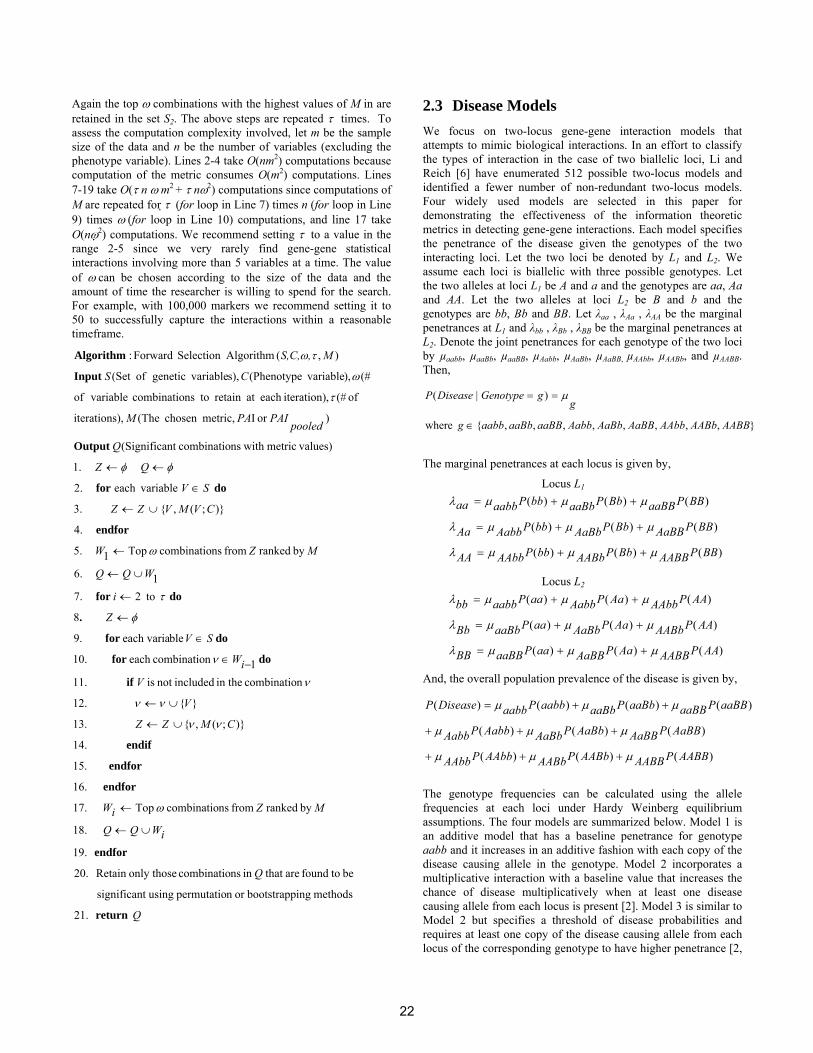
Again the top ω combinations with the highest values of M in are retained in the set S2. The above steps are repeated τ times. To assess the computation complexity involved, let m be the sample size of the data and n be the number of variables (excluding the phenotype variable). Lines 2-4 take O(nm2) computations because computation of the metric consumes O(m2) computations. Lines 7-19 take O(τ n ω m2

+ τ nω2) computations since computations of M are repeated for τ (for loop in Line 7) times n (for loop in Line 9) times ω (for loop in Line 10) computations, and line 17 take O(nω2) computations. We recommend setting τ to a value in the range 2-5 since we very rarely find gene-gene statistical interactions involving more than 5 variables at a time. The value of ω can be chosen according to the size of the data and the amount of time the researcher is willing to spend for the search. For example, with 100,000 markers we recommend setting it to 50 to successfully capture the interactions within a reasonable timeframe.

Q

Q

iWQQ

MZiW

CMZZ

V

ViW

SV

Z

i

WQQ

MZW

CVMVZZ

SV

QZ

Q

pooledPAIPAM

CS

M,S,C,

21.

methods ingbootstrappor n permutatio usingt significan

be tofound are that in nscombinatio only thoseRetain 20.

19.

18.

by ranked from nscombinatio Top 17.

16.

.15

14.

)};(,{ .13

}{ 12.

n combinatio in the includednot is 11.

1n combinatioeach 10.

bleeach varia .9

8

to2 7.1 6.

by ranked from nscombinatio Top1.5

.4

)};(,{.3

variableeach.2

.1

values)metric with nscombinationt (Significa

)or I metric,chosen (The ),iterations

of (#,iteration)each at retain tonscombinatio variableof

(#), variable(Phenotypes), variablegenetic of(Set

),( Algorithm Selection Forward :

return

endfor

endfor

endfor

endif

if

dofor

dofor

.

dofor

endfor

dofor

Output

Input

Algorithm

∪←

←

∪←

∪←

−∈

∈

←

←

∪←

←

∪←

∈

←←

ω

νν

νν

ν

ν

φ

τ

ω

φφ

τ

ω

τω

2.3 Disease Models

We focus on two-locus gene-gene interaction models that attempts to mimic biological interactions. In an effort to classify the types of interaction in the case of two biallelic loci, Li and Reich [6] have enumerated 512 possible two-locus models and identified a fewer number of non-redundant two-locus models. Four widely used models are selected in this paper for demonstrating the effectiveness of the information theoretic metrics in detecting gene-gene interactions. Each model specifies the penetrance of the disease given the genotypes of the two interacting loci. Let the two loci be denoted by L1 and L2. We assume each loci is biallelic with three possible genotypes. Let the two alleles at loci L1 be A and a and the genotypes are aa, Aa and AA. Let the two alleles at loci L2 be B and b and the genotypes are bb, Bb and BB. Let λaa , λAa , λAA be the marginal penetrances at L1 and λbb , λBb , λBB be the marginal penetrances at L2. Denote the joint penetrances for each genotype of the two loci by µaabb, µaaBb, µaaBB, µAabb, µAaBb, µAaBB, µAAbb, µAABb, and µAABB. Then,

},,,,,,,,{ where

)|(

AABBAABbAAbbAaBBAaBbAabbaaBBaaBbaabbg

ggGenotypeDiseaseP

∈

== μ

The marginal penetrances at each locus is given by,

)()()(

)()()(

)()()(

BBPAABBBbPAABbbbPAAbbAA

BBPAaBBBbPAaBbbbPAabbAa

BBPaaBBBbPaaBbbbPaabbaa

μμμλ

μμμλ

μμμλ

++=

++=

++=

)()()(

)()()(

)()()(

AAPAABBAaPAaBBaaPaaBBBB

AAPAABbAaPAaBbaaPaaBbBb

AAPAAbbAaPAabbaaPaabbbb

μμμλ

μμμλ

μμμλ

++=

++=

++=

And, the overall population prevalence of the disease is given by,

)()()(

)()()(

)()()()(

AABBPAABBAABbPAABbAAbbPAAbb

AaBBPAaBBAaBbPAaBbAabbPAabb

aaBBPaaBBaaBbPaaBbaabbPaabbDiseaseP

μμμ

μμμ

μμμ

+++

+++

++=

The genotype frequencies can be calculated using the allele frequencies at each loci under Hardy Weinberg equilibrium assumptions. The four models are summarized below. Model 1 is an additive model that has a baseline penetrance for genotype aabb and it increases in an additive fashion with each copy of the disease causing allele in the genotype. Model 2 incorporates a multiplicative interaction with a baseline value that increases the chance of disease multiplicatively when at least one disease causing allele from each locus is present [2]. Model 3 is similar to Model 2 but specifies a threshold of disease probabilities and requires at least one copy of the disease causing allele from each locus of the corresponding genotype to have higher penetrance [2,

Locus L1

Locus L2

22

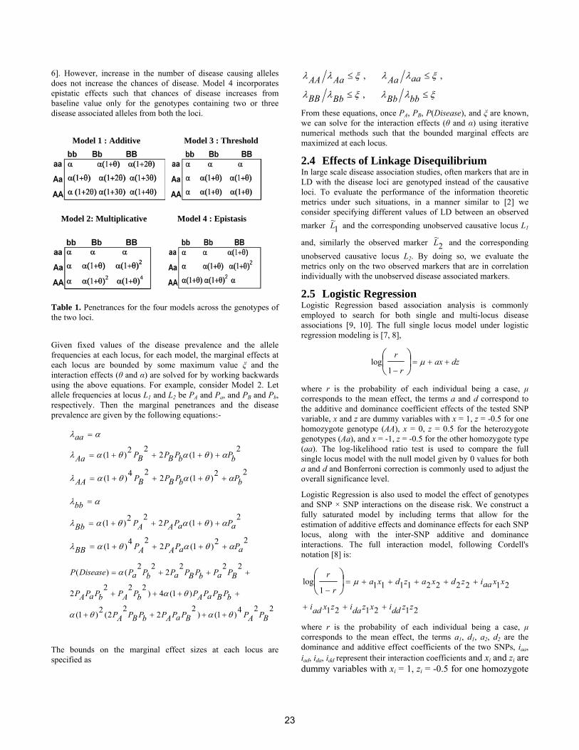
6]. However, increase in the number of disease causing alleles does not increase the chances of disease. Model 4 incorporates epistatic effects such that chances of disease increases from baseline value only for the genotypes containing two or three disease associated alleles from both the loci.

Model 2: Multiplicative Model 4 : Epistasis

Table 1. Penetrances for the four models across the genotypes of the two loci. Given fixed values of the disease prevalence and the allele frequencies at each locus, for each model, the marginal effects at each locus are bounded by some maximum value ξ and the interaction effects (θ and α) are solved for by working backwards using the above equations. For example, consider Model 2. Let allele frequencies at locus L1 and L2 be PA and Pa, and PB and Pb, respectively. Then the marginal penetrances and the disease prevalence are given by the following equations:-

22)1(224)1(

2)1(2

22)1(

bPbPBPBPAA

bPbPBPBPAa

aa

αθαθαλ

αθαθαλ

αλ

++++=

++++=

=

22)1(224)1(

2)1(2

22)1(

aPaPAPAPBB

aPaPAPAPBb

bb

αθαθαλ

αθαθαλ

αλ

++++=

++++=

=

224)1( )2

22

2(2)1(

)1(4)222

2

222

222

()(

BPAPBPaPAPbPBPAP

bPBPaPAPbPAPbPaPAP

BPaPbPBPaPbPaPDiseaseP

θαθα

θα

α

++++

++++

+++=

The bounds on the marginal effect sizes at each locus are specified as

ξλλξλλ

ξλλξλλ

≤≤

≤≤

bbBbBbBB

aaAaAaAA,

,,

From these equations, once PA, PB, P(Disease), and ξ are known, we can solve for the interaction effects (θ and α) using iterative numerical methods such that the bounded marginal effects are maximized at each locus.

2.4 Effects of Linkage Disequilibrium In large scale disease association studies, often markers that are in LD with the disease loci are genotyped instead of the causative loci. To evaluate the performance of the information theoretic metrics under such situations, in a manner similar to [2] we consider specifying different values of LD between an observed marker 1

~L and the corresponding unobserved causative locus L1

and, similarly the observed marker 2~L and the corresponding

unobserved causative locus L2. By doing so, we evaluate the metrics only on the two observed markers that are in correlation individually with the unobserved disease associated markers.

2.5 Logistic Regression Logistic Regression based association analysis is commonly employed to search for both single and multi-locus disease associations [9, 10]. The full single locus model under logistic regression modeling is [7, 8],

dzaxr

r++=

−⎟⎠⎞

⎜⎝⎛

μ1

log

where r is the probability of each individual being a case, μ corresponds to the mean effect, the terms a and d correspond to the additive and dominance coefficient effects of the tested SNP variable, x and z are dummy variables with x = 1, z = -0.5 for one homozygote genotype (AA), x = 0, z = 0.5 for the heterozygote genotypes (Aa), and x = -1, z = -0.5 for the other homozygote type (aa). The log-likelihood ratio test is used to compare the full single locus model with the null model given by 0 values for both a and d and Bonferroni correction is commonly used to adjust the overall significance level.

Logistic Regression is also used to model the effect of genotypes and SNP × SNP interactions on the disease risk. We construct a fully saturated model by including terms that allow for the estimation of additive effects and dominance effects for each SNP locus, along with the inter-SNP additive and dominance interactions. The full interaction model, following Cordell's notation [8] is:

212121

21222211111log

zzddixzdaizxadi

xxaaizdxazdxar

r

+++

+++++=−

⎟⎠⎞

⎜⎝⎛

μ

where r is the probability of each individual being a case, μ corresponds to the mean effect, the terms a1, d1, a2, d2 are the dominance and additive effect coefficients of the two SNPs, iaa, iad, ida, idd represent their interaction coefficients and xi and zi are dummy variables with xi = 1, zi = -0.5 for one homozygote

Model 1 : Additive Model 3 : Threshold

23

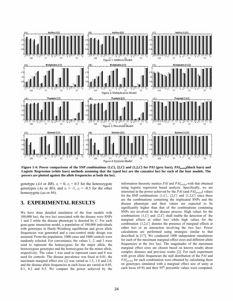
Figure 1-4: Power comparisons of the SNP combinations {1,C}, {2,C} and {1,2,C} for PAI (grey bars), PAIpooled(black bars) and Logistic Regression (white bars) methods assuming that the typed loci are the causative loci for each of the four models. The powers are plotted against the allele frequencies at both the loci.

genotype (AA or BB), xi = 0, zi = 0.5 for the heterozygote genotypes (Aa or Bb), and xi = -1, zi = -0.5 for the other homozygote (aa or bb).

3. EXPERIMENTAL RESULTS

We have done detailed simulation of the four models with 100,000 loci, the two loci associated with the disease were SNPs 1 and 2 while the disease phenotype is denoted by C. For each gene-gene interaction model, a population of 100,000 individuals with genotypes in Hardy-Weinberg equilibrium and given allele frequencies was generated and a case-control study design was assumed. From the population, 1000 cases and 1000 controls were randomly selected. For convenience, the values 1, 2, and 3 were used to represent the homozygous for the major allele, the heterozygous genotypes and the homozygous for the minor allele, respectively. The value 1 was used to represent cases and 0 was used for controls. The disease prevalence was fixed at 0.01, the maximum marginal effect size (ξ) was varied as 1.5, 1.8 and 2.0, and the disease allele frequencies at each locus are varied as 0.05, 0.1, 0.2 and 0.5. We compare the power achieved by the

information theoretic metrics PAI and PAIpooled with that obtained using logistic regression based analysis. Specifically, we are interested in the power achieved by the PAI (and PAIpooled) values for the SNP combinations {1,C}, {2,C} and {1,2,C} since these are the combinations containing the implicated SNPs and the disease phenotype and their values are expected to be significantly higher than that of the combinations containing SNPs not involved in the disease process. High values for the combinations {1,C} and {2,C} shall enable the detection of the marginal effects at either loci while high values for the combination {1,2,C} denotes the presence of marginal effects at either loci or an interaction involving the two loci. Power calculations are performed using strategies similar to that described in [17]. We conducted 1000 independent simulations for each of the maximum marginal effect sizes and different allele frequencies at the two loci. The magnitudes of the maximum marginal effect sizes are chosen based on known results about complex diseases and previous works [2]. For each experiment with given allele frequencies the null distribution of the PAI and PAIpooled for each combination were obtained by calculating them on genotypes simulated with a marginal effect size of unity at each locus (θ=0) and their 95th percentile values were computed.

24

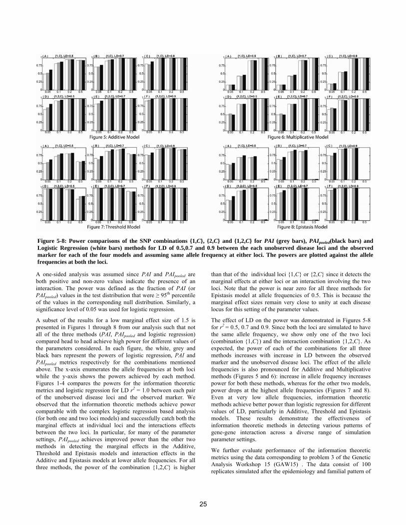
Figure 5-8: Power comparisons of the SNP combinations {1,C}, {2,C} and {1,2,C} for PAI (grey bars), PAIpooled(black bars) and Logistic Regression (white bars) methods for LD of 0.5,0.7 and 0.9 between the each unobserved disease loci and the observed marker for each of the four models and assuming same allele frequency at either loci. The powers are plotted against the allele frequencies at both the loci.

A one-sided analysis was assumed since PAI and PAIpooled are both positive and non-zero values indicate the presence of an interaction. The power was defined as the fraction of PAI (or PAIpooled) values in the test distribution that were ≥ 95th percentile of the values in the corresponding null distribution. Similarly, a significance level of 0.05 was used for logistic regression.

A subset of the results for a low marginal effect size of 1.5 is presented in Figures 1 through 8 from our analysis such that not all of the three methods (PAI, PAIpooled and logistic regression) compared head to head achieve high power for different values of the parameters considered. In each figure, the white, grey and black bars represent the powers of logistic regression, PAI and PAIpooled metrics respectively for the combinations mentioned above. The x-axis enumerates the allele frequencies at both loci while the y-axis shows the powers achieved by each method. Figures 1-4 compares the powers for the information theoretic metrics and logistic regression for LD r2 = 1.0 between each pair of the unobserved disease loci and the observed marker. We observed that the information theoretic methods achieve power comparable with the complex logistic regression based analysis (for both one and two loci models) and successfully catch both the marginal effects at individual loci and the interactions effects between the two loci. In particular, for many of the parameter settings, PAIpooled achieves improved power than the other two methods in detecting the marginal effects in the Additive, Threshold and Epistasis models and interaction effects in the Additive and Epistasis models at lower allele frequencies. For all three methods, the power of the combination {1,2,C} is higher

than that of the individual loci {1,C} or {2,C} since it detects the marginal effects at either loci or an interaction involving the two loci. Note that the power is near zero for all three methods for Epistasis model at allele frequencies of 0.5. This is because the marginal effect sizes remain very close to unity at each disease locus for this setting of the parameter values.

The effect of LD on the power was demonstrated in Figures 5-8 for r2 = 0.5, 0.7 and 0.9. Since both the loci are simulated to have the same allele frequency, we show only one of the two loci (combination {1,C}) and the interaction combination {1,2,C}. As expected, the power of each of the combinations for all three methods increases with increase in LD between the observed marker and the unobserved disease loci. The effect of the allele frequencies is also pronounced for Additive and Multiplicative methods (Figures 5 and 6): increase in allele frequency increases power for both these methods, whereas for the other two models, power drops at the highest allele frequencies (Figures 7 and 8). Even at very low allele frequencies, information theoretic methods achieve better power than logistic regression for different values of LD, particularly in Additive, Threshold and Epistasis models. These results demonstrate the effectiveness of information theoretic methods in detecting various patterns of gene-gene interaction across a diverse range of simulation parameter settings.

We further evaluate performance of the information theoretic metrics using the data corresponding to problem 3 of the Genetic Analysis Workshop 15 (GAW15) . The data consist of 100 replicates simulated after the epidemiology and familial pattern of

25

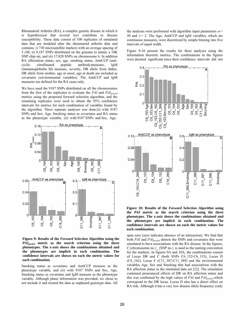
Rheumatoid Arthritis (RA), a complex genetic disease in which it is hypothesized that several loci contribute to disease susceptibility. These data consist of 100 replicates of simulated data that are modeled after the rheumatoid arthritis data and contains: i) 730 microsatellite markers with an average spacing of 5 cM; ii) 9,187 SNPs distributed on the genome to mimic a 10K SNP chip set, and iii) 17,820 SNPs on chromosome 6. In addition RA affectation status, sex, age, smoking status, AntiCCP (anti-cyclic citrullinated peptide antibody)measure, IgM (immunoglobulin M) measure, severity, DR allele from father, DR allele from mother, age at onset, age at death are included as covariates (environmental variables). The AntiCCP and IgM measures are defined for the RA cases only.

We have used the 9187 SNPs distributed on all the chromosomes from the first of the replicates to evaluate the PAI and PAIpooled metrics using the proposed forward selection algorithm, and the remaining replicates were used to obtain the 95% confidence intervals for metrics for each combination of variables found by the algorithm. Three separate analyses was done:(i) with 9187 SNPs and Sex, Age, Smoking status as covariates and RA status as the phenotype variable, (ii) with 9187 SNPs and Sex, Age,

Smoking status as covariates and AntiCCP measure as the phenotype variable, and (ii) with 9187 SNPs and Sex, Age, Smoking status as covariates and IgM measure as the phenotype variable. Although phase information was provided, we chose to not include it and treated the data as unphased genotype data. All

the analyses were performed with algorithm input parameters ω = 50 and τ = 2. The Age, AntiCCP and IgM variables, which are continuous measures, were discretized by simple binning into five intervals of equal width.

Figure 9-10 present the results for three analyses using the information theoretic metrics. The combinations in the figures were deemed significant since their confidence intervals did not

span zero (zero indicates absence of an interaction). We find that both PAI and PAIpooled detects the SNPs and covariates that were simulated to have associations with the RA disease. In the figures, C{chromosome no.}_{SNP no.} is used as the naming convention for the markers. In figures 9A and 10A, the combinations consist of Locus DR and C (both SNPs C6_152-C6_155), Locus D (C6_162), Locus F (C11_387-C11_389) and the environmental variables Age, Sex and Smoking that had associations with the RA affection status in the simulated data set [22]. The simulation contained pronounced effects of DR on RA affection status and this was confirmed by the high values of PAI and PAIpooled which correspond to the DR locus. Locus D also has a direct effect on RA risk. Although it has a very low disease allele frequency (only

Figure 9: Results of the Forward Selection Algorithm using the PAIpooled metric as the search criterion using the three phenotypes. The x-axis shows the combinations obtained and the phenotypes are implicit in each combination. The confidence intervals are shown on each the metric values for each combination.

Figure 10: Results of the Forward Selection Algorithm using the PAI metric as the search criterion using the three phenotypes. The x-axis shows the combinations obtained and the phenotypes are implicit in each combination. The confidence intervals are shown on each the metric values for each combination.

26

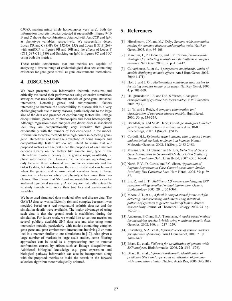
0.0083, making minor allele homozygotes very rare), both the information theoretic metrics detected it successfully. Figure 9-10 B and C shows the combinations obtained with AntiCCP and IgM as phenotype variables, respectively. We successfully detect Locus DR and C (SNPs C6_152-C6_155) and Locus E (C18_269) with AntiCCP in figures 9B and 10B and the effects of Locus F (C11_387-C11_389) and Smoking on IgM in figures 9C and 10C using both the metrics.

These results demonstrate that our metrics are capable of analyzing a diverse range of epidemiological data sets containing evidences for gene-gene as well as gene-environment interactions.

4. DISCUSSION

We have presented two information theoretic measures and critically evaluated their performances using extensive simulation strategies that uses four different models of gene-gene statistical interaction. Detecting genes and environmental; factors interacting to increase the susceptibility to disease risk is a very challenging task due to many reasons, particularly due to the large size of the data and presence of confounding factors like linkage disequilibrium, presence of phenocopies and locus heterogeneity. Although regression based analyses can detect disease associated loci, they are computationally very intensive that grows exponentially with the number of loci considered in the model. Information theoretic methods have high power in detecting gene-gene interactions and have the advantage of being simpler and computationally faster. We do not intend to claim that our proposed metrics are the best since the properties of each method depends greatly on the factors like sample size, type of the interactions involved, density of the genetic maps, availability of phase information etc. However the metrics are appealing not only because they performed well in the experiments and the GAW15 data, but also because they are flexible and can be used when the genetic and environmental variables have different numbers of classes or when the phenotype has more than two classes. This means that SNP and microsatellite markers can be analyzed together if necessary. Also they are naturally extensible to study models with more than two loci and environmental variables.

We have used simulated data modeled after real disease data. The GAW15 data set was sufficiently rich and complex because it was modeled based on a real rheumatoid arthritis data set and the simulation details were available. The major advantage of using such data is that the ground truth is established during the simulation. For future work, we would like to test our metrics on several publicly available SNP data sets and also using more interaction models, particularly with models containing complex gene-gene and gene-environment interactions involving 3 or more loci in a manner similar to our simulations in [17]. Also given a large number of markers in large scale studies, some filtering approaches can be used as a preprocessing step to remove confounders caused by effects such as linkage disequilibrium. Additional biological knowledge e.g. gene expression and biological pathway information can also be incorporated along with the proposed metrics to make the search in the forward selection algorithm more biologically oriented.

5. References [1] Hirschhcorn, J.N. and M.J. Daly, Genome-wide association

studies for common diseases and complex traits. Nat Rev Genet, 2005. 6: p. 95-108.

[2] Marchini, J., P. Donnelly, and L.R. Cardon, Genome-wide strategies for detecting multiple loci that influence complex diseases. Nat Genet, 2005. 37: p. 413-417.

[3] Culverhouse, R., et al., A perspective on epistasis: limits of models displaying no main effects. Am J Hum Genet, 2002. 70(461-471).

[4] Hoh, J. and J. Ott, Mathematical multi-locus approaches to localising complex human trait genes. Nat Rev Genet, 2003. 4: p. 701-709.

[5] Hallgrímsdóttir, I.B. and D.S. S Yuster, A complete classification of epistatic two-locus models. BMC Genetics, 2008. 9(17).

[6] Li, W. and J. Reich, A complete enumeration and classification of two-locus disease models. Hum Hered, 2000. 50: p. 334-339.

[7] Barhdadi, A. and M.-P. Dubé, Two-stage strategies to detect gene × gene interactions in case-control data. BMC Proceedings, 2007. 1 (Suppl 1):S135.

[8] Cordell, H.J., Epistasis: what it means, what it doesn’t mean, and statistical methods to detect it in humans. Human Molecular Genetics, 2002. 11(20): p. 2463-2468.

[9] Musani, S.K., D. Shriner, and N. Liu, Detection of Gene x Gene Interactions in Genome-Wide Association Studies of Human Population Data. Hum Hered, 2007. 63: p. 67-84.

[10] North, B.V., D. Curtis, and P.C. Sham, Application of Logistic Regression to Case-Control Association Studies Involving Two Causative Loci. Hum Hered, 2005. 59: p. 79-87.

[11] Liu, Z. and L. T., Multilocus LD measure and tagging SNP selection with generalized mutual information. Genetic Epidemiology 2005. 29: p. 353-364.

[12] Moore, J.H., et al., A flexible computational framework for detecting, characterizing, and interpreting statistical patterns of epistasis in genetic studies of human disease susceptibility. Journal of Theoretical Biology, 2006. 241: p. 252-261.

[13] Anderson, E.C. and E.A. Thompson, A model-based method for identifying species hybrids using multilocus genetic data. Genetics, 2002. 160: p. 1217-1229.

[14] Rosenberg, N.A., et al., Informativeness of genetic markers for inference of ancestry. Am J Hum Genet, 2003. 73: p. 1402-1422.

[15] Bhasi, K., et al., VizStruct for visualization of genome-wide SNP analyses. Bioinformatics, 2006. 22(1569-1576).

[16] Bhasi, K., et al., Information-theoretic identification of predictive SNPs and supervised visualization of genome-wide association studies. Nucleic Acids Res, 2006. 34(e101).

27

[17] Chanda, P., et al., Information-theoretic metrics for visualizing gene-environment interactions. Am J Hum Genet, 2007. 81: p. 939-963.

[18] Zhao, J., E. Boerwinkle, and M. Xiong, An entropy-based statistic for genomewide association studies. Am J Hum Genet, 2005. 77: p. 27-40.

[19] Genetic Analysis Workshop 15. (http://www.gaworkshop.org/gaw15data.htm) 2006.

[20] Shannon, C.E., A mathematical theory of communication. Bell System Technical Journal, 1948. 27: p. 379-423,623-656.

[21] Han, T.S., Multiple mutual informations and multiple interactions in frequency data. Information and Control, 1980. 46(1): p. 26-45.

[22] Miller, M.B., et al., Genetic Analysis Workshop 15: Simulation of a complex genetic model for rheumatoid arthritis in nuclear families including a dense SNP map with linkage disequilibrium between marker loci and trait loci. BMC Genetics, 2007.

28

A fast, large-scale learning method for protein sequenceclassification

Pavel Kuksa, Pai-Hsi Huang, Vladimir Pavlovic∗

Department of Computer ScienceRutgers University

Piscataway, NJ 08854{pkuksa;paihuang;vladimir}@cs.rutgers.edu

ABSTRACT

Motivation: Establishing structural and functional rela-tionships between sequences in the presence of only the pri-mary sequence information is a key task in biological se-quence analysis. This ability can be critical for tasks suchas making inferences of the structural class of unannotatedproteins when no secondary or tertiary structure is avail-able. Recent computational methods based on profile andmismatch neighborhood kernels have significantly improvedone’s ability to elucidate such relationships. However, theneed for additional reduction in computational complexityand improvement in predictive accuracy hinders the widespreaduse of these powerful computational tools.Results: We present a new general approach for sequenceanalysis based on a class of efficient string-based kernels,sparse spatial sample kernels (SSSK). The approach offersstate-of-the-art accuracy for sequence classification, low com-putational cost, and scales well with the size of sequencedatabases, in both supervised and semi-supervised learningsettings. Application of the proposed methods to a remotehomology detection and a fold recognition problems yieldsperformance equal to or better than existing state-of-the-artalgorithms. We also demonstrate the benefit of the spatialinformation and multi-resolution sampling for achieving thisaccuracy and for discriminative sequence motif discovery.The proposed methods can be applied to very large partially-labeled databases of protein sequences because of low com-putational complexity and show substantial improvementsin computing time over the existing methods.Availability: Supplementary data and Matlab/C codes areavailable at http://seqam.rutgers.edu/spatial-kernels/Contact: vladimir@cs.rutgers.edu

Categories and Subject Descriptors

I.2 [Artificial Intelligence]: Learning; I.5 [Pattern Recog-nition]: Applications; I.5.2. [Pattern Recognition]: De-

∗corresponding author

Permission to make digital or hard copies of all or part of this work forpersonal or classroom use is granted without fee provided that copies arenot made or distributed for profit or commercial advantage and that copiesbear this notice and the full citation on the first page. To copy otherwise, torepublish, to post on servers or to redistribute to lists, requires prior specificpermission and/or a fee.BIOKDD ’08 Las Vegas, Nevada, USACopyright 2008 ACM 978-1-60558-302-0/08/0008 ...$5.00.

sign Methodology

General Terms

Algorithms, Design, Measurement, Performance, Experimen-tation

Keywords

sequence classification, large-scale semi-supervised learning,string kernels

1. INTRODUCTIONClassification of protein sequences into structural or func-

tional classes is a fundamental problem in computationalbiology. With the advent of large-scale sequencing tech-niques, experimental elucidation of an unknown protein se-quence function becomes an expensive and tedious task.Currently, there are more than 61 million DNA sequencesin GenBank [3], and approximately 349,480 annotated and5.3 million unannotated sequences in UNIPROT [2], makingdevelopment of computational aids for sequence annotationa critical and timely task. In this work we focus on pro-tein sequence classification problems using only the primarysequence information. While additional sources of informa-tion, such as the secondary or tertiary structure, may lessenthe burden of establishing the homology, they may often beunavailable or difficult to acquire for new putative proteins.

Early approaches to computationally-aided homology de-tection, such as BLAST [1] and FASTA [22], rely on aligningthe query sequence to a database of known sequences (pair-wise alignment). Later methods, such as profiles [7] andprofile hidden Markov models (profile HMM) [6], collect ag-gregate statistics from a group of sequences known to belongto the same family. Such generative approaches only makeuse of positive training examples, while the discriminativeapproaches attempt to capture the distinction between dif-ferent classes by considering both positive and negative ex-amples. In many sequence analysis tasks, the discriminativemethods such as kernel-based [25] machine learning meth-ods provide the most accurate results [4, 13, 17, 24]. Severaltypes of kernels for protein homology detection have beenproposed over the last decade. In [11], Jaakkola et al. pro-posed SVMFisher, derived from probabilistic models. Leslieet al. in [17] proposed a class of kernels that operate directlyon strings and derive features from the sequence content.Both classes of kernels demonstrated improved discrimina-tive power over methods that operate under generative set-tings.

29

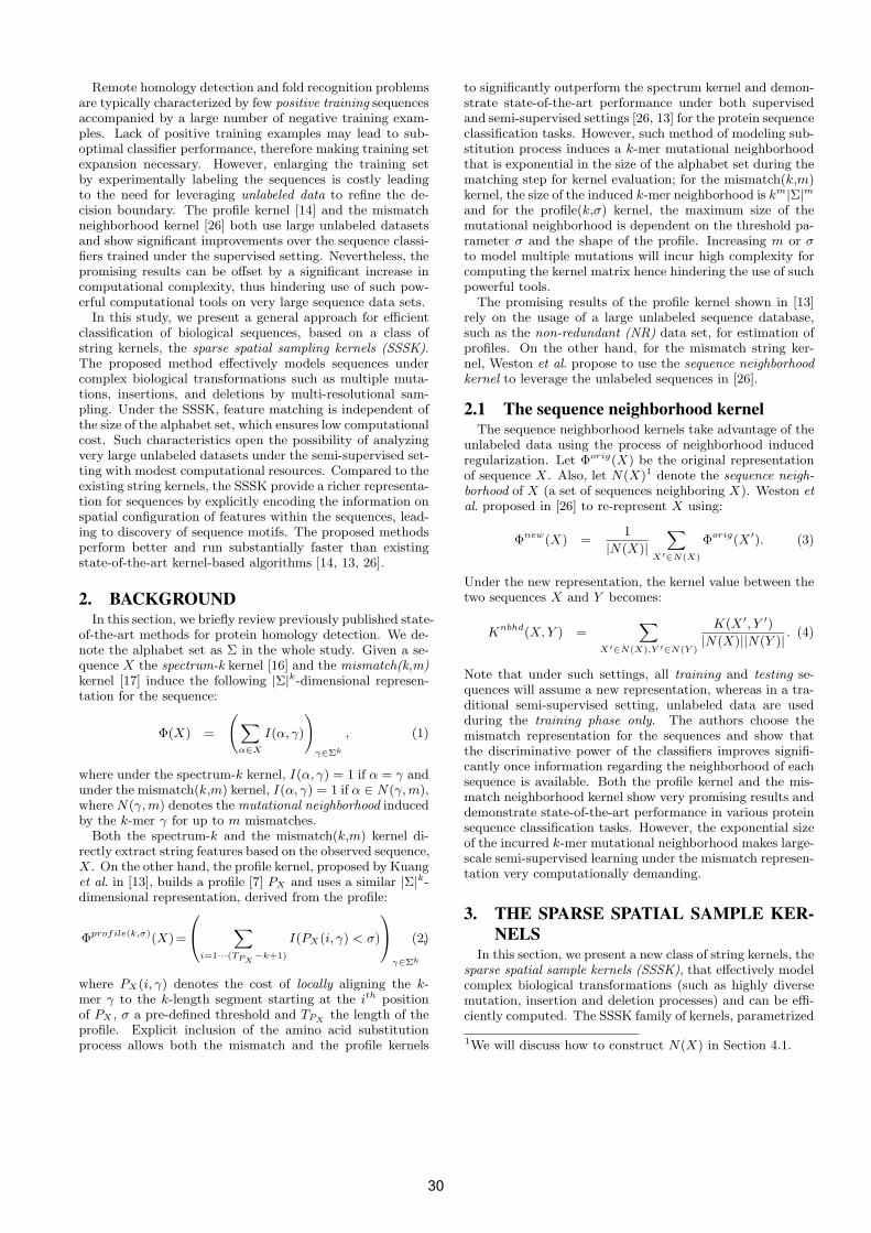
Remote homology detection and fold recognition problemsare typically characterized by few positive training sequencesaccompanied by a large number of negative training exam-ples. Lack of positive training examples may lead to sub-optimal classifier performance, therefore making training setexpansion necessary. However, enlarging the training setby experimentally labeling the sequences is costly leadingto the need for leveraging unlabeled data to refine the de-cision boundary. The profile kernel [14] and the mismatchneighborhood kernel [26] both use large unlabeled datasetsand show significant improvements over the sequence classi-fiers trained under the supervised setting. Nevertheless, thepromising results can be offset by a significant increase incomputational complexity, thus hindering use of such pow-erful computational tools on very large sequence data sets.

In this study, we present a general approach for efficientclassification of biological sequences, based on a class ofstring kernels, the sparse spatial sampling kernels (SSSK).The proposed method effectively models sequences undercomplex biological transformations such as multiple muta-tions, insertions, and deletions by multi-resolutional sam-pling. Under the SSSK, feature matching is independent ofthe size of the alphabet set, which ensures low computationalcost. Such characteristics open the possibility of analyzingvery large unlabeled datasets under the semi-supervised set-ting with modest computational resources. Compared to theexisting string kernels, the SSSK provide a richer representa-tion for sequences by explicitly encoding the information onspatial configuration of features within the sequences, lead-ing to discovery of sequence motifs. The proposed methodsperform better and run substantially faster than existingstate-of-the-art kernel-based algorithms [14, 13, 26].

2. BACKGROUNDIn this section, we briefly review previously published state-

of-the-art methods for protein homology detection. We de-note the alphabet set as Σ in the whole study. Given a se-quence X the spectrum-k kernel [16] and the mismatch(k,m)kernel [17] induce the following |Σ|k-dimensional represen-tation for the sequence:

Φ(X) =

X

α∈X

I(α, γ)

!

γ∈Σk

, (1)

where under the spectrum-k kernel, I(α, γ) = 1 if α = γ andunder the mismatch(k,m) kernel, I(α, γ) = 1 if α ∈ N(γ, m),where N(γ, m) denotes the mutational neighborhood inducedby the k-mer γ for up to m mismatches.

Both the spectrum-k and the mismatch(k,m) kernel di-rectly extract string features based on the observed sequence,X. On the other hand, the profile kernel, proposed by Kuanget al. in [13], builds a profile [7] PX and uses a similar |Σ|k-dimensional representation, derived from the profile:

Φprofile(k,σ)(X)=

0

@

X

i=1···(TPX−k+1)

I(PX(i, γ) < σ)

1

A

γ∈Σk

,(2)

where PX(i, γ) denotes the cost of locally aligning the k-mer γ to the k-length segment starting at the ith positionof PX , σ a pre-defined threshold and TPX

the length of theprofile. Explicit inclusion of the amino acid substitutionprocess allows both the mismatch and the profile kernels

to significantly outperform the spectrum kernel and demon-strate state-of-the-art performance under both supervisedand semi-supervised settings [26, 13] for the protein sequenceclassification tasks. However, such method of modeling sub-stitution process induces a k-mer mutational neighborhoodthat is exponential in the size of the alphabet set during thematching step for kernel evaluation; for the mismatch(k,m)kernel, the size of the induced k-mer neighborhood is km|Σ|m

and for the profile(k,σ) kernel, the maximum size of themutational neighborhood is dependent on the threshold pa-rameter σ and the shape of the profile. Increasing m or σ

to model multiple mutations will incur high complexity forcomputing the kernel matrix hence hindering the use of suchpowerful tools.

The promising results of the profile kernel shown in [13]rely on the usage of a large unlabeled sequence database,such as the non-redundant (NR) data set, for estimation ofprofiles. On the other hand, for the mismatch string ker-nel, Weston et al. propose to use the sequence neighborhoodkernel to leverage the unlabeled sequences in [26].

2.1 The sequence neighborhood kernelThe sequence neighborhood kernels take advantage of the

unlabeled data using the process of neighborhood inducedregularization. Let Φorig(X) be the original representationof sequence X. Also, let N(X)1 denote the sequence neigh-borhood of X (a set of sequences neighboring X). Weston etal. proposed in [26] to re-represent X using:

Φnew(X) =1

|N(X)|

X

X′∈N(X)

Φorig(X ′). (3)

Under the new representation, the kernel value between thetwo sequences X and Y becomes:

Knbhd(X, Y ) =

X

X′∈N(X),Y ′∈N(Y )

K(X ′, Y ′)

|N(X)||N(Y )|. (4)

Note that under such settings, all training and testing se-quences will assume a new representation, whereas in a tra-ditional semi-supervised setting, unlabeled data are usedduring the training phase only. The authors choose themismatch representation for the sequences and show thatthe discriminative power of the classifiers improves signifi-cantly once information regarding the neighborhood of eachsequence is available. Both the profile kernel and the mis-match neighborhood kernel show very promising results anddemonstrate state-of-the-art performance in various proteinsequence classification tasks. However, the exponential sizeof the incurred k-mer mutational neighborhood makes large-scale semi-supervised learning under the mismatch represen-tation very computationally demanding.

3. THE SPARSE SPATIAL SAMPLE KER-

NELSIn this section, we present a new class of string kernels, the

sparse spatial sample kernels (SSSK), that effectively modelcomplex biological transformations (such as highly diversemutation, insertion and deletion processes) and can be effi-ciently computed. The SSSK family of kernels, parametrized

1We will discuss how to construct N(X) in Section 4.1.

30

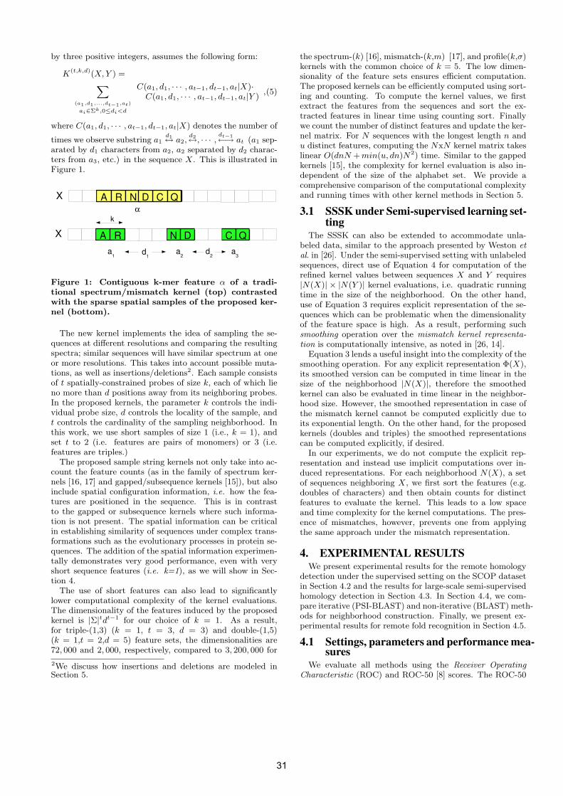
by three positive integers, assumes the following form:

K(t,k,d)(X, Y ) =

X

(a1,d1,...,dt−1,at)

ai∈Σk,0≤di<d

C(a1, d1, · · · , at−1, dt−1, at|X)·C(a1, d1, · · · , at−1, dt−1, at|Y )

,(5)

where C(a1, d1, · · · , at−1, dt−1, at|X) denotes the number of

times we observe substring a1

d1

↔ a2,d2

↔, · · · ,dt−1

←→ at (a1 sep-arated by d1 characters from a2, a2 separated by d2 charac-ters from a3, etc.) in the sequence X. This is illustrated inFigure 1.

Figure 1: Contiguous k-mer feature α of a tradi-tional spectrum/mismatch kernel (top) contrastedwith the sparse spatial samples of the proposed ker-nel (bottom).

The new kernel implements the idea of sampling the se-quences at different resolutions and comparing the resultingspectra; similar sequences will have similar spectrum at oneor more resolutions. This takes into account possible muta-tions, as well as insertions/deletions2. Each sample consistsof t spatially-constrained probes of size k, each of which lieno more than d positions away from its neighboring probes.In the proposed kernels, the parameter k controls the indi-vidual probe size, d controls the locality of the sample, andt controls the cardinality of the sampling neighborhood. Inthis work, we use short samples of size 1 (i.e., k = 1), andset t to 2 (i.e. features are pairs of monomers) or 3 (i.e.features are triples.)

The proposed sample string kernels not only take into ac-count the feature counts (as in the family of spectrum ker-nels [16, 17] and gapped/subsequence kernels [15]), but alsoinclude spatial configuration information, i.e. how the fea-tures are positioned in the sequence. This is in contrastto the gapped or subsequence kernels where such informa-tion is not present. The spatial information can be criticalin establishing similarity of sequences under complex trans-formations such as the evolutionary processes in protein se-quences. The addition of the spatial information experimen-tally demonstrates very good performance, even with veryshort sequence features (i.e. k=1), as we will show in Sec-tion 4.

The use of short features can also lead to significantlylower computational complexity of the kernel evaluations.The dimensionality of the features induced by the proposedkernel is |Σ|tdt−1 for our choice of k = 1. As a result,for triple-(1,3) (k = 1, t = 3, d = 3) and double-(1,5)(k = 1,t = 2,d = 5) feature sets, the dimensionalities are72, 000 and 2, 000, respectively, compared to 3, 200, 000 for

2We discuss how insertions and deletions are modeled inSection 5.

the spectrum-(k) [16], mismatch-(k,m) [17], and profile(k,σ)kernels with the common choice of k = 5. The low dimen-sionality of the feature sets ensures efficient computation.The proposed kernels can be efficiently computed using sort-ing and counting. To compute the kernel values, we firstextract the features from the sequences and sort the ex-tracted features in linear time using counting sort. Finallywe count the number of distinct features and update the ker-nel matrix. For N sequences with the longest length n andu distinct features, computing the NxN kernel matrix takeslinear O(dnN + min(u, dn)N2) time. Similar to the gappedkernels [15], the complexity for kernel evaluation is also in-dependent of the size of the alphabet set. We provide acomprehensive comparison of the computational complexityand running times with other kernel methods in Section 5.

3.1 SSSK under Semi-supervised learning set-ting

The SSSK can also be extended to accommodate unla-beled data, similar to the approach presented by Weston etal. in [26]. Under the semi-supervised setting with unlabeledsequences, direct use of Equation 4 for computation of therefined kernel values between sequences X and Y requires|N(X)| × |N(Y )| kernel evaluations, i.e. quadratic runningtime in the size of the neighborhood. On the other hand,use of Equation 3 requires explicit representation of the se-quences which can be problematic when the dimensionalityof the feature space is high. As a result, performing suchsmoothing operation over the mismatch kernel representa-tion is computationally intensive, as noted in [26, 14].

Equation 3 lends a useful insight into the complexity of thesmoothing operation. For any explicit representation Φ(X),its smoothed version can be computed in time linear in thesize of the neighborhood |N(X)|, therefore the smoothedkernel can also be evaluated in time linear in the neighbor-hood size. However, the smoothed representation in case ofthe mismatch kernel cannot be computed explicitly due toits exponential length. On the other hand, for the proposedkernels (doubles and triples) the smoothed representationscan be computed explicitly, if desired.

In our experiments, we do not compute the explicit rep-resentation and instead use implicit computations over in-duced representations. For each neighborhood N(X), a setof sequences neighboring X, we first sort the features (e.g.doubles of characters) and then obtain counts for distinctfeatures to evaluate the kernel. This leads to a low spaceand time complexity for the kernel computations. The pres-ence of mismatches, however, prevents one from applyingthe same approach under the mismatch representation.

4. EXPERIMENTAL RESULTSWe present experimental results for the remote homology

detection under the supervised setting on the SCOP datasetin Section 4.2 and the results for large-scale semi-supervisedhomology detection in Section 4.3. In Section 4.4, we com-pare iterative (PSI-BLAST) and non-iterative (BLAST) meth-ods for neighborhood construction. Finally, we present ex-perimental results for remote fold recognition in Section 4.5.

4.1 Settings, parameters and performance mea-sures

We evaluate all methods using the Receiver OperatingCharacteristic (ROC) and ROC-50 [8] scores. The ROC-50

31

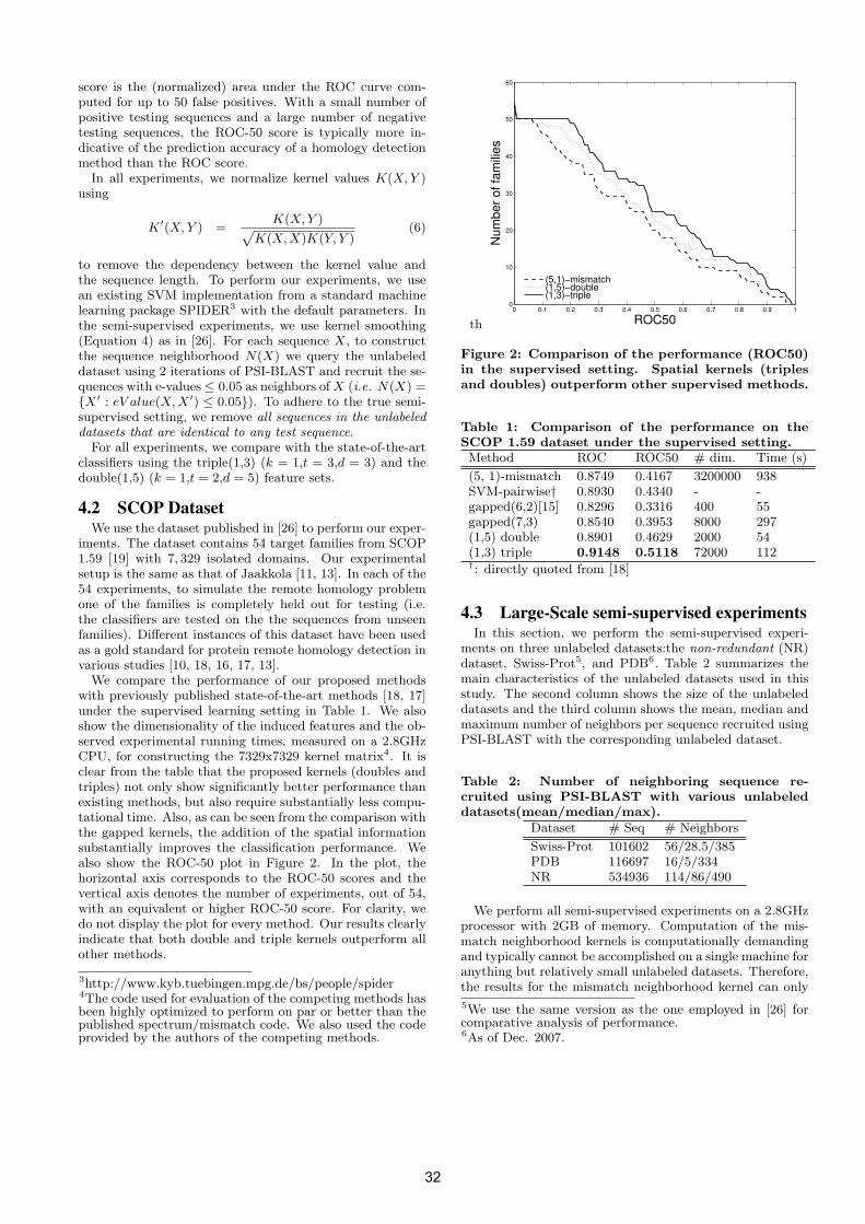
score is the (normalized) area under the ROC curve com-puted for up to 50 false positives. With a small number ofpositive testing sequences and a large number of negativetesting sequences, the ROC-50 score is typically more in-dicative of the prediction accuracy of a homology detectionmethod than the ROC score.

In all experiments, we normalize kernel values K(X, Y )using

K′(X, Y ) =

K(X, Y )p

K(X, X)K(Y, Y )(6)

to remove the dependency between the kernel value andthe sequence length. To perform our experiments, we usean existing SVM implementation from a standard machinelearning package SPIDER3 with the default parameters. Inthe semi-supervised experiments, we use kernel smoothing(Equation 4) as in [26]. For each sequence X, to constructthe sequence neighborhood N(X) we query the unlabeleddataset using 2 iterations of PSI-BLAST and recruit the se-quences with e-values≤ 0.05 as neighbors of X (i.e. N(X) ={X ′ : eV alue(X, X ′) ≤ 0.05}). To adhere to the true semi-supervised setting, we remove all sequences in the unlabeleddatasets that are identical to any test sequence.

For all experiments, we compare with the state-of-the-artclassifiers using the triple(1,3) (k = 1,t = 3,d = 3) and thedouble(1,5) (k = 1,t = 2,d = 5) feature sets.

4.2 SCOP DatasetWe use the dataset published in [26] to perform our exper-

iments. The dataset contains 54 target families from SCOP1.59 [19] with 7, 329 isolated domains. Our experimentalsetup is the same as that of Jaakkola [11, 13]. In each of the54 experiments, to simulate the remote homology problemone of the families is completely held out for testing (i.e.the classifiers are tested on the the sequences from unseenfamilies). Different instances of this dataset have been usedas a gold standard for protein remote homology detection invarious studies [10, 18, 16, 17, 13].

We compare the performance of our proposed methodswith previously published state-of-the-art methods [18, 17]under the supervised learning setting in Table 1. We alsoshow the dimensionality of the induced features and the ob-served experimental running times, measured on a 2.8GHzCPU, for constructing the 7329x7329 kernel matrix4. It isclear from the table that the proposed kernels (doubles andtriples) not only show significantly better performance thanexisting methods, but also require substantially less compu-tational time. Also, as can be seen from the comparison withthe gapped kernels, the addition of the spatial informationsubstantially improves the classification performance. Wealso show the ROC-50 plot in Figure 2. In the plot, thehorizontal axis corresponds to the ROC-50 scores and thevertical axis denotes the number of experiments, out of 54,with an equivalent or higher ROC-50 score. For clarity, wedo not display the plot for every method. Our results clearlyindicate that both double and triple kernels outperform allother methods.

3http://www.kyb.tuebingen.mpg.de/bs/people/spider4The code used for evaluation of the competing methods hasbeen highly optimized to perform on par or better than thepublished spectrum/mismatch code. We also used the codeprovided by the authors of the competing methods.

th

0 0.1 0.2 0.3 0.4 0.5 0.6 0.7 0.8 0.9 10

10

20

30

40

50

60

ROC50

Num

ber

of fa

mili

es

(5,1)−mismatch(1,5)−double(1,3)−triple

Figure 2: Comparison of the performance (ROC50)in the supervised setting. Spatial kernels (triplesand doubles) outperform other supervised methods.

Table 1: Comparison of the performance on theSCOP 1.59 dataset under the supervised setting.Method ROC ROC50 # dim. Time (s)

(5, 1)-mismatch 0.8749 0.4167 3200000 938SVM-pairwise† 0.8930 0.4340 - -gapped(6,2)[15] 0.8296 0.3316 400 55gapped(7,3) 0.8540 0.3953 8000 297(1,5) double 0.8901 0.4629 2000 54(1,3) triple 0.9148 0.5118 72000 112†: directly quoted from [18]

4.3 Large-Scale semi-supervised experimentsIn this section, we perform the semi-supervised experi-

ments on three unlabeled datasets:the non-redundant (NR)dataset, Swiss-Prot5, and PDB6. Table 2 summarizes themain characteristics of the unlabeled datasets used in thisstudy. The second column shows the size of the unlabeleddatasets and the third column shows the mean, median andmaximum number of neighbors per sequence recruited usingPSI-BLAST with the corresponding unlabeled dataset.

Table 2: Number of neighboring sequence re-cruited using PSI-BLAST with various unlabeleddatasets(mean/median/max).

Dataset # Seq # Neighbors

Swiss-Prot 101602 56/28.5/385PDB 116697 16/5/334NR 534936 114/86/490

We perform all semi-supervised experiments on a 2.8GHzprocessor with 2GB of memory. Computation of the mis-match neighborhood kernels is computationally demandingand typically cannot be accomplished on a single machine foranything but relatively small unlabeled datasets. Therefore,the results for the mismatch neighborhood kernel can only

5We use the same version as the one employed in [26] forcomparative analysis of performance.6As of Dec. 2007.

32

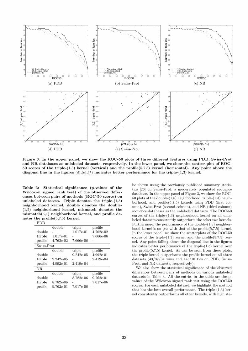
0 0.1 0.2 0.3 0.4 0.5 0.6 0.7 0.8 0.9 15

10

15

20

25

30

35

40

45

50

55

ROC50

Num

ber

of fa

mili

es

(1,5)−double nbhd(1,3)−triple nbhdprofile(5,7.5)

(a) PDB

0 0.1 0.2 0.3 0.4 0.5 0.6 0.7 0.8 0.9 15

10

15

20

25

30

35

40

45

50

55

ROC50

Num

ber

of fa

mili

es

(1,5)−double nbhd(1,3)−triple nbhdprofile(5,7.5)

(b) Swiss-Prot

0 0.1 0.2 0.3 0.4 0.5 0.6 0.7 0.8 0.9 15

10

15

20

25

30

35

40

45

50

55

ROC50

Num

ber

of fa

mili

es

(1,5)−double nbhd(1,3)−triple nbhdprofile(5,7.5)

(c) NR

0 0.1 0.2 0.3 0.4 0.5 0.6 0.7 0.8 0.9 10

0.1

0.2

0.3

0.4

0.5

0.6

0.7

0.8

0.9

1

profile(5,7.5)

(1,3

)−tr

iple

nb

hd

(d) PDB

0 0.1 0.2 0.3 0.4 0.5 0.6 0.7 0.8 0.9 10

0.1

0.2

0.3

0.4

0.5

0.6

0.7

0.8

0.9

1

profile(5,7.5)

(1,3

)−tr

iple

nb

hd

(e) Swiss-Prot

0 0.1 0.2 0.3 0.4 0.5 0.6 0.7 0.8 0.9 10

0.1

0.2

0.3

0.4

0.5

0.6

0.7

0.8

0.9

1

profile(5,7.5)

(1,3

)−tr

iple

nb

hd

(f) NR

Figure 3: In the upper panel, we show the ROC-50 plots of three different features using PDB, Swiss-Protand NR databases as unlabeled datasets, respectively. In the lower panel, we show the scatter-plot of ROC-50 scores of the triple-(1,3) kernel (vertical) and the profile(5,7.5) kernel (horizontal). Any point above thediagonal line in the figures (d),(e),(f) indicates better performance for the triple-(1,3) kernel.

Table 3: Statistical significance (p-values of theWilcoxon signed rank test) of the observed differ-ences between pairs of methods (ROC-50 scores) onunlabeled datasets. Triple denotes the triple-(1,3)neighborhood kernel, double denotes the double-(1,5) neighborhood kernel, mismatch denotes themismatch(5,1) neighborhood kernel, and profile de-notes the profile(5,7.5) kernel.

PDBdouble triple profile

double - 1.017e-01 4.762e-02triple 1.017e-01 - 7.666e-06profile 4.762e-02 7.666e-06 -

Swiss-Protdouble triple profile

double - 9.242e-05 4.992e-01triple 9.242e-05 - 2.419e-04profile 4.992e-01 2.419e-04 -

NRdouble triple profile

double - 8.782e-06 9.762e-01triple 8.782e-06 - 7.017e-06profile 9.762e-01 7.017e-06 -

be shown using the previously published summary statis-tics [26] on Swiss-Prot, a moderately populated sequencedatabase. In the upper panel of Figure 3, we show the ROC-50 plots of the double-(1,5) neighborhood, triple-(1,3) neigh-borhood, and profile(5,7.5) kernels using PDB (first col-umn), Swiss-Prot (second column), and NR (third column)sequence databases as the unlabeled datasets. The ROC-50curves of the triple-(1,3) neighborhood kernel on all unla-beled datasets consistently outperform the other two kernels.Furthermore, the performance of the double-(1,5) neighbor-hood kernel is on par with that of the profile(5,7.5) kernel.In the lower panel, we show the scatterplots of the ROC-50scores of the triple-(1,3) kernel and the profile(5,7.5) ker-nel. Any point falling above the diagonal line in the figuresindicates better performance of the triple-(1,3) kernel overthe profile(5,7.5) kernel. As can be seen from these plots,the triple kernel outperforms the profile kernel on all threedatasets (43/37/34 wins and 4/5/10 ties on PDB, Swiss-Prot, and NR datasets, respectively).

We also show the statistical significance of the observeddifferences between pairs of methods on various unlabeleddatasets in Table 3. All the entries in the table are the p-values of the Wilcoxon signed rank test using the ROC-50scores. For each unlabeled dataset, we highlight the methodthat has the best overall performance. The triple-(1,3) ker-nel consistently outperforms all other kernels, with high sta-

33

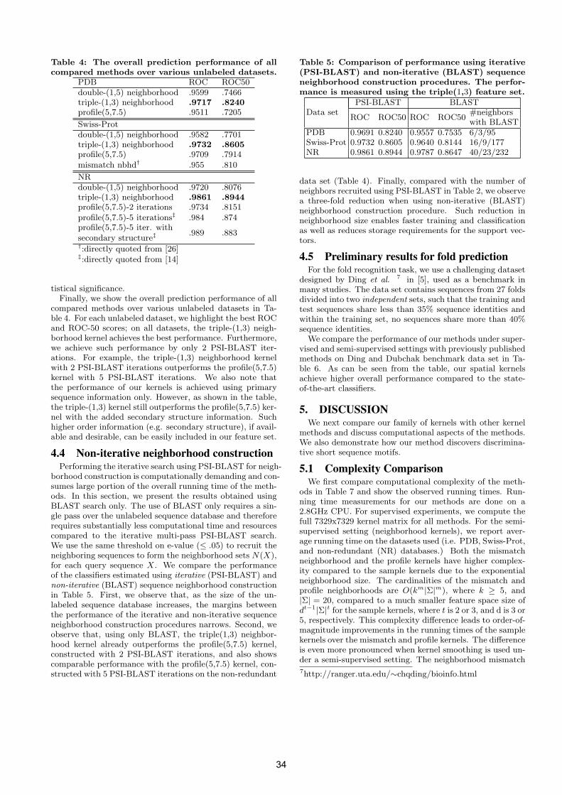
Table 4: The overall prediction performance of allcompared methods over various unlabeled datasets.

PDB ROC ROC50double-(1,5) neighborhood .9599 .7466triple-(1,3) neighborhood .9717 .8240profile(5,7.5) .9511 .7205

Swiss-Protdouble-(1,5) neighborhood .9582 .7701triple-(1,3) neighborhood .9732 .8605profile(5,7.5) .9709 .7914mismatch nbhd† .955 .810

NRdouble-(1,5) neighborhood .9720 .8076triple-(1,3) neighborhood .9861 .8944profile(5,7.5)-2 iterations .9734 .8151profile(5,7.5)-5 iterations‡ .984 .874profile(5,7.5)-5 iter. withsecondary structure‡

.989 .883

†:directly quoted from [26]‡:directly quoted from [14]

tistical significance.Finally, we show the overall prediction performance of all

compared methods over various unlabeled datasets in Ta-ble 4. For each unlabeled dataset, we highlight the best ROCand ROC-50 scores; on all datasets, the triple-(1,3) neigh-borhood kernel achieves the best performance. Furthermore,we achieve such performance by only 2 PSI-BLAST iter-ations. For example, the triple-(1,3) neighborhood kernelwith 2 PSI-BLAST iterations outperforms the profile(5,7.5)kernel with 5 PSI-BLAST iterations. We also note thatthe performance of our kernels is achieved using primarysequence information only. However, as shown in the table,the triple-(1,3) kernel still outperforms the profile(5,7.5) ker-nel with the added secondary structure information. Suchhigher order information (e.g. secondary structure), if avail-able and desirable, can be easily included in our feature set.

4.4 Non-iterative neighborhood constructionPerforming the iterative search using PSI-BLAST for neigh-

borhood construction is computationally demanding and con-sumes large portion of the overall running time of the meth-ods. In this section, we present the results obtained usingBLAST search only. The use of BLAST only requires a sin-gle pass over the unlabeled sequence database and thereforerequires substantially less computational time and resourcescompared to the iterative multi-pass PSI-BLAST search.We use the same threshold on e-value (≤ .05) to recruit theneighboring sequences to form the neighborhood sets N(X),for each query sequence X. We compare the performanceof the classifiers estimated using iterative (PSI-BLAST) andnon-iterative (BLAST) sequence neighborhood constructionin Table 5. First, we observe that, as the size of the un-labeled sequence database increases, the margins betweenthe performance of the iterative and non-iterative sequenceneighborhood construction procedures narrows. Second, weobserve that, using only BLAST, the triple(1,3) neighbor-hood kernel already outperforms the profile(5,7.5) kernel,constructed with 2 PSI-BLAST iterations, and also showscomparable performance with the profile(5,7.5) kernel, con-structed with 5 PSI-BLAST iterations on the non-redundant

Table 5: Comparison of performance using iterative(PSI-BLAST) and non-iterative (BLAST) sequenceneighborhood construction procedures. The perfor-mance is measured using the triple(1,3) feature set.

Data setPSI-BLAST BLAST

ROC ROC50 ROC ROC50#neighborswith BLAST

PDB 0.9691 0.8240 0.9557 0.7535 6/3/95Swiss-Prot 0.9732 0.8605 0.9640 0.8144 16/9/177NR 0.9861 0.8944 0.9787 0.8647 40/23/232

data set (Table 4). Finally, compared with the number ofneighbors recruited using PSI-BLAST in Table 2, we observea three-fold reduction when using non-iterative (BLAST)neighborhood construction procedure. Such reduction inneighborhood size enables faster training and classificationas well as reduces storage requirements for the support vec-tors.

4.5 Preliminary results for fold predictionFor the fold recognition task, we use a challenging dataset

designed by Ding et al. 7 in [5], used as a benchmark inmany studies. The data set contains sequences from 27 foldsdivided into two independent sets, such that the training andtest sequences share less than 35% sequence identities andwithin the training set, no sequences share more than 40%sequence identities.

We compare the performance of our methods under super-vised and semi-supervised settings with previously publishedmethods on Ding and Dubchak benchmark data set in Ta-ble 6. As can be seen from the table, our spatial kernelsachieve higher overall performance compared to the state-of-the-art classifiers.

5. DISCUSSIONWe next compare our family of kernels with other kernel

methods and discuss computational aspects of the methods.We also demonstrate how our method discovers discrimina-tive short sequence motifs.

5.1 Complexity ComparisonWe first compare computational complexity of the meth-

ods in Table 7 and show the observed running times. Run-ning time measurements for our methods are done on a2.8GHz CPU. For supervised experiments, we compute thefull 7329x7329 kernel matrix for all methods. For the semi-supervised setting (neighborhood kernels), we report aver-age running time on the datasets used (i.e. PDB, Swiss-Prot,and non-redundant (NR) databases.) Both the mismatchneighborhood and the profile kernels have higher complex-ity compared to the sample kernels due to the exponentialneighborhood size. The cardinalities of the mismatch andprofile neighborhoods are O(km|Σ|m), where k ≥ 5, and|Σ| = 20, compared to a much smaller feature space size ofdt−1|Σ|t for the sample kernels, where t is 2 or 3, and d is 3 or5, respectively. This complexity difference leads to order-of-magnitude improvements in the running times of the samplekernels over the mismatch and profile kernels. The differenceis even more pronounced when kernel smoothing is used un-der a semi-supervised setting. The neighborhood mismatch

7http://ranger.uta.edu/∼chqding/bioinfo.html

34

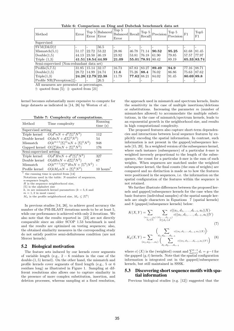
Table 6: Comparison on Ding and Dubchak benchmark data set

Method ErrorTop 5Error

BalancedError

Top 5BalancedError

RecallTop 5Recall

PrecisionTop 5Precision

F1Top5F1

SupervisedSVM(D&D)† - - 56.5 - - - - - - -Mismatch(5,1) 51.17 22.72 53.22 28.86 46.78 71.14 90.52 95.25 61.68 81.45Double(1,5) 44.13 23.50 46.19 23.92 53.81 76.18 61.90 79.85 57.57 77.97Triple (1,3) 41.51 18.54 44.99 21.09 55.01 78.91 80.42 89.19 65.33 83.74Semi-supervised (Non-redundant data set)Profile(5,7.5) 31.85 15.14 32.17 16.73 67.83 83.27 89.49 94.9 77.16 88.71Double(1,5) 28.72 14.99 24.74 11.6 75.26 88.4 76.02 86.86 75.63 87.62Triple(1,3) 24.28 12.79 22.38 11.79 77.62 88.21 84.02 91.45 80.69 89.8Profile NR(Perceptron)‡ - - 26.5 - - - - - - -All measures are presented as percentages.†: quoted from [5]; ‡: quoted from [21]

kernel becomes substantially more expensive to compute forlarge datasets as indicated in [14, 26] by Weston et al. .

Table 7: Complexity of computations.

Method Time complexityRunningtime (s)

Supervised setting

Triple kernel O(d2nN + d2|Σ|3N2) 112Double kernel O(dnN + d|Σ|2N2) 54Mismatch O(km+1|Σ|mnN + |Σ|kN2) 948Gapped kernel O(

`

g

k

´

knN + |Σ|kN2) 176Semi-supervised setting

Triple kernel O(d2HnN + d2|Σ|3N2) 327Double kernel O(dHnN + d|Σ|2N2) 67Mismatch O(km+1|Σ|mHnN + |Σk|N2) -Profile kernel O(kMσnN + |Σ|kN2) 10 hours†

†the running time is quoted from [14]

Notations used in the table: N-number of sequences,n-sequence length,H is the sequence neighborhood size,|Σ| is the alphabet sizek, m are mismatch kernel parameters (k = 5, 6 andm = 1, 2 in most cases)

Mσ is the profile neighborhood size, Mσ ≤ |Σk|

In previous studies [14, 26], to achieve good accuracy thenumber of the PSI-BLAST iterations needs to be at least 5,while our performance is achieved with only 2 iterations. Wealso note that the results reported in [23] are not directlycomparable since an older SCOP 1.53 benchmark is usedand the results are optimized on testing sequences; also,the obtained similarity measures in the corresponding studydo not satisfy positive semi-definiteness condition (are notMercer kernels).

5.2 Biological motivationThe feature sets induced by our kernels cover segments

of variable length (e.g., 2 − 6 residues in the case of thedouble-(1, 5) kernel). On the other hand, the mismatch andprofile kernels cover segments of fixed length (e.g., 5 or 6residues long) as illustrated in Figure 1. Sampling at dif-ferent resolutions also allows one to capture similarity inthe presence of more complex substitution, insertion, anddeletion processes, whereas sampling at a fixed resolution,

the approach used in mismatch and spectrum kernels, limitsthe sensitivity in the case of multiple insertions/deletionsor substitutions. Increasing the parameter m (number ofmismatches allowed) to accommodate the multiple substi-tutions, in the case of mismatch/spectrum kernels, leads toan exponential growth in the neighborhood size, and resultsin high computational complexity.

The proposed features also capture short-term dependen-cies and interactions between local sequence features by ex-plicitly encoding the spatial information. In contrast, suchinformation is not present in the gapped/subsequence ker-nels [15, 20]. In a weighted version of the subsequence kernel,where each instance (subsequence) of a particular k-mer isweighted inversely proportional to the length of the subse-quence, the count for a particular k-mer is the sum of suchweights. When sequences are matched under the weightedsubsequence kernel, the final counts (the sum of weights) arecompared and no distinction is made as to how the featureswere positioned in the sequences, i.e. the information on thespatial configuration of the features within the sequence isnot retained.

We further illustrate differences between the proposed ker-nels and gapped/subsequence kernels for the case when thebasic features (individual samples) of the spatial sample ker-nels are single characters in Equations 7 (spatial kernels)and 8 (gapped/subsequence kernels) below:

K(X, Y ) =X

(a1,...,at)

ai∈Σ

X

(d1,...,dt−1)

0≤di<d

c((a1, d1, . . . , dt−1, at)|X)·c((a1, d1, . . . , dt−1, at)|Y )

(7)

Kg(X, Y ) =X

(a1,a2,...,at)

“

X

d1,d2,...,dt−1

c((a1,d1,...,dt−1,at)|X)

”

·

“

X

d1,d2,...,dt−1

c((a1,d1,...,dt−1,at)|Y )

” (8)

where c(·|X) is the (weighted) count andPt−1

i=1di = g−t for

the gapped (g, t) kernels. Note that the spatial configurationinformation is integrated out in the gapped/subsequencekernels, but still maintained in SSSK.

5.3 Discovering short sequence motifs with spa-tial information

Previous biological studies (e.g. [12]) suggested that the

35

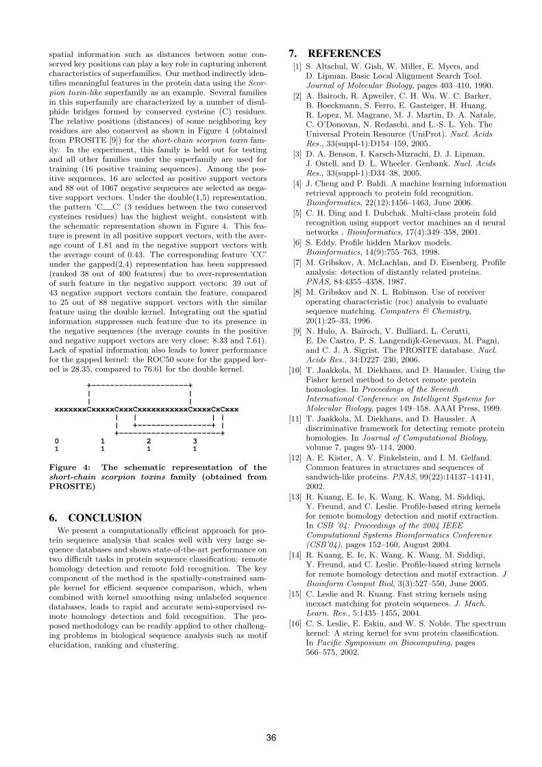
spatial information such as distances between some con-served key positions can play a key role in capturing inherentcharacteristics of superfamilies. Our method indirectly iden-tifies meaningful features in the protein data using the Scor-pion toxin-like superfamily as an example. Several familiesin this superfamily are characterized by a number of disul-phide bridges formed by conserved cysteine (C) residues.The relative positions (distances) of some neighboring keyresidues are also conserved as shown in Figure 4 (obtainedfrom PROSITE [9]) for the short-chain scorpion toxin fam-ily. In the experiment, this family is held out for testingand all other families under the superfamily are used fortraining (16 positive training sequences). Among the pos-itive sequences, 16 are selected as positive support vectorsand 88 out of 1067 negative sequences are selected as nega-tive support vectors. Under the double(1,5) representation,the pattern ’C C’ (3 residues between the two conservedcysteines residues) has the highest weight, consistent withthe schematic representation shown in Figure 4. This fea-ture is present in all positive support vectors, with the aver-age count of 1.81 and in the negative support vectors withthe average count of 0.43. The corresponding feature ’CC’under the gapped(2,4) representation has been suppressed(ranked 38 out of 400 features) due to over-representationof such feature in the negative support vectors: 39 out of43 negative support vectors contain the feature, comparedto 25 out of 88 negative support vectors with the similarfeature using the double kernel. Integrating out the spatialinformation suppresses such feature due to its presence inthe negative sequences (the average counts in the positiveand negative support vectors are very close: 8.33 and 7.61).Lack of spatial information also leads to lower performancefor the gapped kernel: the ROC50 score for the gapped ker-nel is 28.35, compared to 76.61 for the double kernel.

+−−−−−−−−−−−−−−−−−−−−−+

| |

| |

xxxxxxxCxxxxxCxxxCxxxxxxxxxxxCxxxxCxCxxx

| | | |

| +−−−−−−−−−−−−−−−−+ |

+−−−−−−−−−−−−−−−−−−−−−−+

0 1 2 3

1 1 1 1

Figure 4: The schematic representation of theshort-chain scorpion toxins family (obtained fromPROSITE)

6. CONCLUSIONWe present a computationally efficient approach for pro-

tein sequence analysis that scales well with very large se-quence databases and shows state-of-the-art performance ontwo difficult tasks in protein sequence classification: remotehomology detection and remote fold recognition. The keycomponent of the method is the spatially-constrained sam-ple kernel for efficient sequence comparison, which, whencombined with kernel smoothing using unlabeled sequencedatabases, leads to rapid and accurate semi-supervised re-mote homology detection and fold recognition. The pro-posed methodology can be readily applied to other challeng-ing problems in biological sequence analysis such as motifelucidation, ranking and clustering.

7. REFERENCES[1] S. Altschul, W. Gish, W. Miller, E. Myers, and

D. Lipman. Basic Local Alignment Search Tool.Journal of Molecular Biology, pages 403–410, 1990.

[2] A. Bairoch, R. Apweiler, C. H. Wu, W. C. Barker,B. Boeckmann, S. Ferro, E. Gasteiger, H. Huang,R. Lopez, M. Magrane, M. J. Martin, D. A. Natale,C. O’Donovan, N. Redaschi, and L.-S. L. Yeh. TheUniversal Protein Resource (UniProt). Nucl. AcidsRes., 33(suppl-1):D154–159, 2005.

[3] D. A. Benson, I. Karsch-Mizrachi, D. J. Lipman,J. Ostell, and D. L. Wheeler. Genbank. Nucl. AcidsRes., 33(suppl-1):D34–38, 2005.

[4] J. Cheng and P. Baldi. A machine learning informationretrieval approach to protein fold recognition.Bioinformatics, 22(12):1456–1463, June 2006.

[5] C. H. Ding and I. Dubchak. Multi-class protein foldrecognition using support vector machines an d neuralnetworks . Bioinformatics, 17(4):349–358, 2001.

[6] S. Eddy. Profile hidden Markov models.Bioinformatics, 14(9):755–763, 1998.

[7] M. Gribskov, A. McLachlan, and D. Eisenberg. Profileanalysis: detection of distantly related proteins.PNAS, 84:4355–4358, 1987.

[8] M. Gribskov and N. L. Robinson. Use of receiveroperating characteristic (roc) analysis to evaluatesequence matching. Computers & Chemistry,20(1):25–33, 1996.

[9] N. Hulo, A. Bairoch, V. Bulliard, L. Cerutti,E. De Castro, P. S. Langendijk-Genevaux, M. Pagni,and C. J. A. Sigrist. The PROSITE database. Nucl.Acids Res., 34:D227–230, 2006.

[10] T. Jaakkola, M. Diekhans, and D. Haussler. Using theFisher kernel method to detect remote proteinhomologies. In Proceedings of the SeventhInternational Conference on Intelligent Systems forMolecular Biology, pages 149–158. AAAI Press, 1999.

[11] T. Jaakkola, M. Diekhans, and D. Haussler. Adiscriminative framework for detecting remote proteinhomologies. In Journal of Computational Biology,volume 7, pages 95–114, 2000.

[12] A. E. Kister, A. V. Finkelstein, and I. M. Gelfand.Common features in structures and sequences ofsandwich-like proteins. PNAS, 99(22):14137–14141,2002.

[13] R. Kuang, E. Ie, K. Wang, K. Wang, M. Siddiqi,Y. Freund, and C. Leslie. Profile-based string kernelsfor remote homology detection and motif extraction.In CSB ’04: Proceedings of the 2004 IEEEComputational Systems Bioinformatics Conference(CSB’04), pages 152–160, August 2004.

[14] R. Kuang, E. Ie, K. Wang, K. Wang, M. Siddiqi,Y. Freund, and C. Leslie. Profile-based string kernelsfor remote homology detection and motif extraction. JBioinform Comput Biol, 3(3):527–550, June 2005.

[15] C. Leslie and R. Kuang. Fast string kernels usinginexact matching for protein sequences. J. Mach.Learn. Res., 5:1435–1455, 2004.

[16] C. S. Leslie, E. Eskin, and W. S. Noble. The spectrumkernel: A string kernel for svm protein classification.In Pacific Symposium on Biocomputing, pages566–575, 2002.

36

[17] C. S. Leslie, E. Eskin, J. Weston, and W. S. Noble.Mismatch string kernels for svm protein classification.In NIPS, pages 1417–1424, 2002.

[18] L. Liao and W. S. Noble. Combining pairwisesequence similarity and support vector machines forremote protein homology detection. In RECOMB,pages 225–232, 2002.

[19] L. Lo Conte, B. Ailey, T. Hubbard, S. Brenner,A. Murzin, and C. Chothia. SCOP: a structuralclassification of proteins database. Nucleic Acids Res.,28:257–259, 2000.

[20] H. Lodhi, C. Saunders, J. Shawe-Taylor,N. Cristianini, and C. Watkins. Text classificationusing string kernels. J. Mach. Learn. Res., 2:419–444,2002.

[21] I. Melvin, E. Ie, J. Weston, W. S. Noble, and C. Leslie.Multi-class protein classification using adaptive codes.J. Mach. Learn. Res., 8:1557–1581, 2007.

[22] W. Pearson and D. Lipman. Improved tools forbiological sequence comparison. PNAS, 85:2444–2448,1988.

[23] H. Rangwala and G. Karypis. Profile-based directkernels for remote homology detection and foldrecognition. Bioinformatics, 21(23):4239–4247, 2005.

[24] S. Sonnenburg, G. Ratsch, and B. Scholkopf. Largescale genomic sequence svm classifiers. In ICML ’05:Proceedings of the 22nd international conference onMachine learning, pages 848–855, New York, NY,USA, 2005.

[25] V. N. Vapnik. Statistical Learning Theory.Wiley-Interscience, 1998.

[26] J. Weston, C. Leslie, E. Ie, D. Zhou, A. Elisseeff, andW. S. Noble. Semi-supervised protein classificationusing cluster kernels. Bioinformatics,21(15):3241–3247, 2005.

37

Catching Old Influenza Virus with A New Markov Model

HamChing LamDept. of Computer Science and Engineering

University of MinnesotaMinneapolis, Minnesota 55455, USA

hamching@cs.umn.edu

Daniel BoleyDept. of Computer Science and Engineering

University of MinnesotaMinneapolis, Minnesota 55455, USA

boley@cs.umn.edu

ABSTRACTWe have developed a novel Markov model which modelsthe genetic distance between viruses based on the Hemag-glutinin (HA) gene, a major surface antigen of the avianinfluenza virus. Using this model we estimate the prob-ability of finding highly similar virus sequences separatedby long time gaps. Our biological assumption is based onneutral evolutionary theory, which has been applied previ-ously to study this virus [Gojobori, Moriyama, and Kimura.PNAS Vol 87. 1990]. Our working hypothesis is that aftera long enough time gap and with the high mutation rateusually found in RNA viruses, many site mutations shouldaccumulate, leading to distinct modern variants. We ob-tained 3439 HA protein sequences isolated through years1918 to 2006 from around the globe, aligned them to a con-sensus sequence using the NCBI alignment tool, and useda Hamming distance metric on the aligned sequences. Wetested our hypothesis by combining a standard Poisson pro-cess with a Markov model. The Poisson process models theoccurrences of mutations in a given time interval, and theMarkov model estimates the probabilities of changes to thegenetic distances due to mutations. By coalescing all se-quences at a given genetic distance to a single state, weobtain a tractable Markov chain with a number of statesequal to the length of the base peptide sequence. The modelpredicts that the probability of finding highly similar virusafter several decades is extremely small. The existence of re-cent viruses which are very similar to older viruses suggeststhat potentially there exists some reservoir which preservesviruses over long periods.

KeywordsInfluenza virus, Poisson process, Markov Model

1. INTRODUCTIONFor the past century researchers have been studying in-

fluenza viruses (IV). Belonging to the viral family Orthomyx-oviridae, influenza viruses have eight unique RNA segments

Permission to make digital or hard copies of all or part of this work forpersonal or classroom use is granted without fee provided that copies arenot made or distributed for profit or commercial advantage and that copiesbear this notice and the full citation on the first page. To copy otherwise, torepublish, to post on servers or to redistribute to lists, requires prior specificpermission and/or a fee.BIOKDD ’08 Las Vegas, Nevada USACopyright 2008 ACM ISBN 978-1-60558-302-0 ...$5.00.

[20] that encode 10 different gene products (PB1 polymerase,PB2 polymerase, PA polymerases, Hemagglutinin (HA), Nu-cleoprotein (NP), Neuraminidase (NA), Matrix M1 and M2proteins, and Nonstructural NS1 and NS2 proteins). Thetarget of our study is the Hemagglutinin HA gene product.We have developed a novel Markov model which models thegenetic distance between viruses based on the Hemagglu-tinin (HA) gene, a major surface antigen of the avian in-fluenza virus. Our working hypothesis is that after a longenough time gap, many site mutations should accumulatein the virus due to a lack of a proofreading function [6],leading to distinct modern variants. We based our biolog-ical assumption on neutral theory of evolution [7, 12, 17,8] and that each amino acid site is under a neutral muta-tion pressure. Previous studies have shown that subtypesof influenza virus are subjected to higher silent substitutionrate [7, 24], which is consistent with the neutral theory ofmolecular evolution. Although their studies were conductedusing nucleotide sequences, we believe that the same gen-eral concept and framework can be applied to study proteinsequences of this virus under this evolutionary assumption.We test our hypothesis by combining a standard Poissonprocess with the Markov model. The Poisson process mod-els the occurrences of mutations in a given time interval, andthe Markov model estimates the probabilities of changes tothe genetic distances due to mutations. We show that itis highly unlikely that very similar sequences would ariselong after the original sequence. Given the observations ofseveral pairs of very similar sequences separated by severaldecades, we conclude that there must be some reservoir orevolutionary mechanism that is capable of preserving oldvirus strains, allowing them to reappear after extended timeintervals.

2. MATERIALS AND METHODS

2.1 Protein Sequence Data and ProcessingThe HA protein is the major surface antigen of the in-

fluenza virus. Its role is to bind to host cell receptors pro-moting fusion between the viron envelope and the host cell[20]. Influenza A virus HA genes have been classified into16 subtypes (H1-H16) according to their antigenic proper-ties. This HA protein is cleaved into two peptide chainsHA1 and HA2 respectively when matured [19]. The HA2chain has been found to vary less and is more conservedcompared to HA1 chain [10]. The HA1 chain is 329 residueslong and is the immunogenic part of HA protein. Past stud-ies have shown that HA1 is undergoing continual diversify-

38

ing change [5, 14] and is the most variable portion of theinfluenza genome[16].

Using the NCBI Influenza database available online [23],we have collected 3439 influenza virus type A protein se-quences deposited before December, 2007 (excluding iden-tical sequences and lab strains/NIAID FLU project). Thiscollection of protein sequences contains isolates from aroundthe globe and from a diverse range of hosts. We used pro-tein sequences because they were known to give more re-liable results than nucleotide sequences when constructingevolutionary history [19]. Each of the 3439 sequences hasa unique annotation which contains the host organism, thestrain number, the year of isolation, subtype, and proteinname. We aligned all sequences to a consensus sequenceusing the NCBI alignment tool. According to the study pre-sented by [16], a uniform consensus strain tends to circulatefor some time, since the mutations that occur during repli-cation do not become fixed in the early stages of circulating.The aligned sequence data were then used with a geneticdistance function to determine the pairwise genetic distance(including gaps) of the sequences.

The genetic distance between two sequences can be thoughtof as the “edit” distance, which is the number of single letterchanges needed to transform one sequence to the other. Thisyields a simple scoring function assigning a zero to a match-ing amino acid base and a one to a mismatch. The sumof all mismatches is usually called the Hamming distance(k) or Hamming score for the pairwise sequence compari-son. For comparison of very similar biological sequences,this Hamming distance can be used under the assumptionthat the observed difference between a pair of sites repre-sents one mutation [3]. The present study could also becarried out using BLAST or any alignment algorithm, butas considerably greater expense. In [15], Hamming distancewas successfully used to find interesting clusters of IV HAsequences and to predict vaccine strains with good results.Hamming distance as genetic distance between viruses hasalso been used effectively in modeling influenza viruses [18].In our study, we compute the Hamming distance based ona consensus alignment to account for the small number ofinsertions and deletions. We then store the pairwise Ham-ming distance scores of HA gene in a pairwise affinity matrixand identify virus sequence pairs sharing high sequence sim-ilarity (at least 90 percent) but separated by a long timegap.

2.2 Markov modelWe model all mutations as the combination of several sin-

gle point mutations and use a Poisson process to model themutation rate. The Poisson process naturally admits morecomplex mutations, treating them as several single pointmutations occurring in rapid succession. Then we build acompact Markov model to model the mutations themselves.Markov models have proven to be a powerful tool for phy-logenetic inference and hypothesis testing when modelingtransitions between amino acid states. Modeling amino acidtransitions is complex since proteins are made of twentyamino acids. Because of this, we take a very different ap-proach in building our Markov model. We are trying to avoida Markov chain where each sequence is a state because thiswould give rise to an exponentially large number of states(20n where n is the number of sites). In our Markov model,we collect into a single state Hk all the protein sequences

0

B

B

B

B

B

@

0 1x1 y1 z1 0

. . .. . .

. . .

0 xn−1 yn−1 zn−1

xn yn

1

C

C

C

C

C

A

Figure 1: Markov transition matrix

at given Hamming distance k from the starting sequences0 ∈ H0. The starting sequence s0 can be chosen either asthe earliest isolated sequence or the most recent one as longas a large time gap is observed when comparing to othersequences. Our Markov model assigns the probability of anarbitrary HA sequence s1 ∈ Hk mutating into a different HAsequence s2 ∈ Hl through a single point mutation, where l

must be one of k − 1, k, k + 1.Previous studies [4, 13] have shown that to better fit the

model, active sites should be excluded in the analysis underthe neutral theory framework. Here we have taken the sameapproach where we have limited the mutations captured byour Markov chain to the HA1 domain consisting of n = 329sites, since this region is less conserved than the HA2 region[15, 14]. Therefore, our Markov model has only n + 1 = 330states instead of the 20n states it would have if we kept eachstate and each possible transition separate.

Formally, consider a finite set of states labeled {H0, ..., Hn}.In order to keep the Markov chain to a manageable size, wegroup all the sequences within Hamming distance of k froma start sequence into a single“super state”Hk. At each tran-sition, we assume a single point mutation occurs, and thatthis mutation of amino acid replacement exhibits uniformrate of evolution throughout long periods of evolutionarytime [25]. This assumption is particularly consistent withthe concept of ”molecular evolutionary clock” and is centralto the neutral theory [1, 7, 22]. Because of the high rate atwhich RNA viruses evolve, it has been observed that thesesequences show the typical pattern of neutral evolution [7].

We denote by a the size of the alphabet of amino acids,in our case 20. For a sequence s1 ∈ Hk, there is a probabil-ity k/n that the mutation occurs in one of the k positionswhere s1 differs from s0, and if this change occurs, there isa 1/(a − 1) chance that the new amino acid in this positionwill match that in the same position of s0. Hence the prob-ability xk of a transition from Hk to Hk−1 is xk = k

n· 1

a−1.

Similar reasoning yields the probability yk that a transitionwill remain at the same Hamming distance: yk = k

n· a−2

a−1.

The probability that mutation will be in one of the n − k

sites that still match s0 is zk = 1 − kn, corresponding to

a transition from Hk to Hk+1. The resulting probabilitiesxk, yk, zk are assembled into a Markov transition matrix M

shown in Figure 1. The entries in each row of M add up to1.

Using this model, we can compute the probability qt thata virus will have a Hamming distance at most k from theinitial source sequence after t mutations. We give the gen-eral form of how to compute the above probability. Welet vt = (vt0, vt1, . . . , vtn) be the row vector of probabili-ties of being in state H0, H1, . . . , Hn, respectively, after t

mutations. At t = 0 we are in state H0 consisting of justthe initial sequence. This is represented by the row vector

39

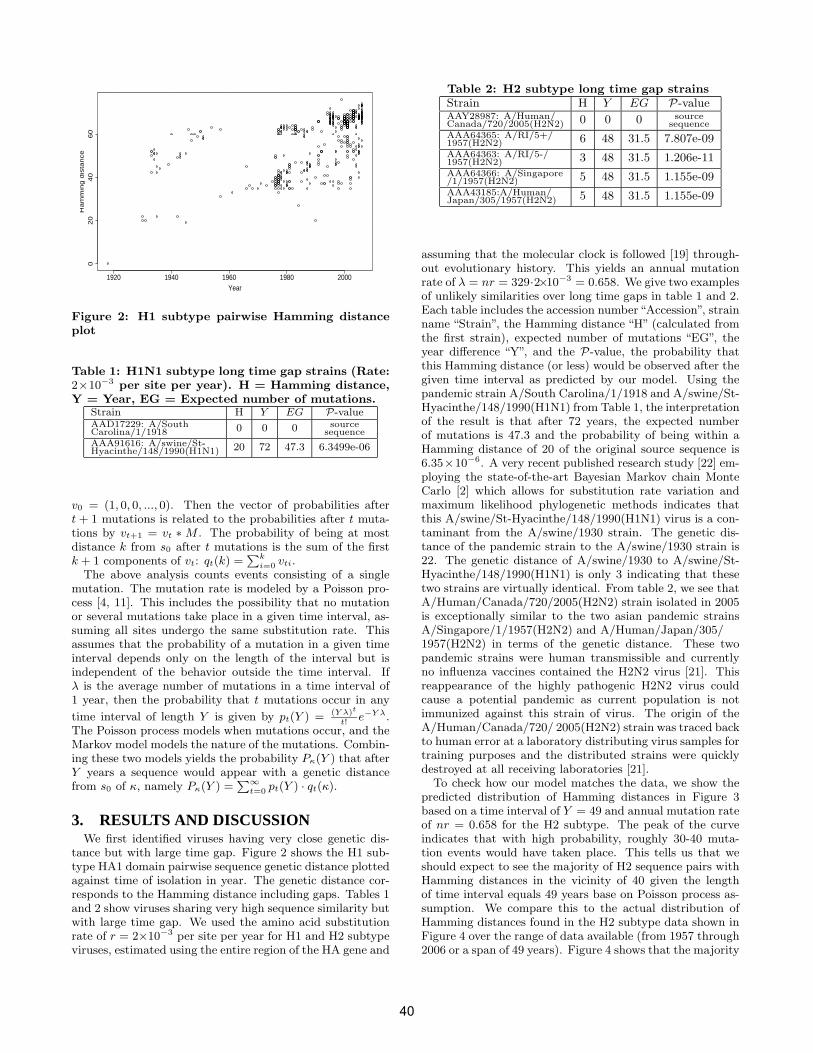
1920 1940 1960 1980 2000

02

04

06

0

Year

Ha

mm

ing

dis

tan

ce

Figure 2: H1 subtype pairwise Hamming distanceplot

Table 1: H1N1 subtype long time gap strains (Rate:2×10−3 per site per year). H = Hamming distance,Y = Year, EG = Expected number of mutations.

Strain H Y EG P-value

AAD17229: A/SouthCarolina/1/1918 0 0 0

sourcesequence

AAA91616: A/swine/St-Hyacinthe/148/1990(H1N1) 20 72 47.3 6.3499e-06

v0 = (1, 0, 0, ..., 0). Then the vector of probabilities aftert + 1 mutations is related to the probabilities after t muta-tions by vt+1 = vt ∗ M . The probability of being at mostdistance k from s0 after t mutations is the sum of the firstk + 1 components of vt: qt(k) =

Pk

i=0vti.

The above analysis counts events consisting of a singlemutation. The mutation rate is modeled by a Poisson pro-cess [4, 11]. This includes the possibility that no mutationor several mutations take place in a given time interval, as-suming all sites undergo the same substitution rate. Thisassumes that the probability of a mutation in a given timeinterval depends only on the length of the interval but isindependent of the behavior outside the time interval. Ifλ is the average number of mutations in a time interval of1 year, then the probability that t mutations occur in any

time interval of length Y is given by pt(Y ) = (Y λ)t

t!e−Y λ.

The Poisson process models when mutations occur, and theMarkov model models the nature of the mutations. Combin-ing these two models yields the probability Pκ(Y ) that afterY years a sequence would appear with a genetic distancefrom s0 of κ, namely Pκ(Y ) =

P∞

t=0pt(Y ) · qt(κ).

3. RESULTS AND DISCUSSIONWe first identified viruses having very close genetic dis-

tance but with large time gap. Figure 2 shows the H1 sub-type HA1 domain pairwise sequence genetic distance plottedagainst time of isolation in year. The genetic distance cor-responds to the Hamming distance including gaps. Tables 1and 2 show viruses sharing very high sequence similarity butwith large time gap. We used the amino acid substitutionrate of r = 2×10−3 per site per year for H1 and H2 subtypeviruses, estimated using the entire region of the HA gene and

Table 2: H2 subtype long time gap strainsStrain H Y EG P-valueAAY28987: A/Human/Canada/720/2005(H2N2) 0 0 0 source

sequenceAAA64365: A/RI/5+/1957(H2N2) 6 48 31.5 7.807e-09

AAA64363: A/RI/5-/1957(H2N2) 3 48 31.5 1.206e-11

AAA64366: A/Singapore/1/1957(H2N2) 5 48 31.5 1.155e-09

AAA43185:A/Human/Japan/305/1957(H2N2) 5 48 31.5 1.155e-09

assuming that the molecular clock is followed [19] through-out evolutionary history. This yields an annual mutationrate of λ = nr = 329·2×10−3 = 0.658. We give two examplesof unlikely similarities over long time gaps in table 1 and 2.Each table includes the accession number“Accession”, strainname “Strain”, the Hamming distance “H” (calculated fromthe first strain), expected number of mutations “EG”, theyear difference “Y”, and the P-value, the probability thatthis Hamming distance (or less) would be observed after thegiven time interval as predicted by our model. Using thepandemic strain A/South Carolina/1/1918 and A/swine/St-Hyacinthe/148/1990(H1N1) from Table 1, the interpretationof the result is that after 72 years, the expected numberof mutations is 47.3 and the probability of being within aHamming distance of 20 of the original source sequence is6.35×10−6. A very recent published research study [22] em-ploying the state-of-the-art Bayesian Markov chain MonteCarlo [2] which allows for substitution rate variation andmaximum likelihood phylogenetic methods indicates thatthis A/swine/St-Hyacinthe/148/1990(H1N1) virus is a con-taminant from the A/swine/1930 strain. The genetic dis-tance of the pandemic strain to the A/swine/1930 strain is22. The genetic distance of A/swine/1930 to A/swine/St-Hyacinthe/148/1990(H1N1) is only 3 indicating that thesetwo strains are virtually identical. From table 2, we see thatA/Human/Canada/720/2005(H2N2) strain isolated in 2005is exceptionally similar to the two asian pandemic strainsA/Singapore/1/1957(H2N2) and A/Human/Japan/305/1957(H2N2) in terms of the genetic distance. These twopandemic strains were human transmissible and currentlyno influenza vaccines contained the H2N2 virus [21]. Thisreappearance of the highly pathogenic H2N2 virus couldcause a potential pandemic as current population is notimmunized against this strain of virus. The origin of theA/Human/Canada/720/ 2005(H2N2) strain was traced backto human error at a laboratory distributing virus samples fortraining purposes and the distributed strains were quicklydestroyed at all receiving laboratories [21].

To check how our model matches the data, we show thepredicted distribution of Hamming distances in Figure 3based on a time interval of Y = 49 and annual mutation rateof nr = 0.658 for the H2 subtype. The peak of the curveindicates that with high probability, roughly 30-40 muta-tion events would have taken place. This tells us that weshould expect to see the majority of H2 sequence pairs withHamming distances in the vicinity of 40 given the lengthof time interval equals 49 years base on Poisson process as-sumption. We compare this to the actual distribution ofHamming distances found in the H2 subtype data shown inFigure 4 over the range of data available (from 1957 through2006 or a span of 49 years). Figure 4 shows that the majority

40

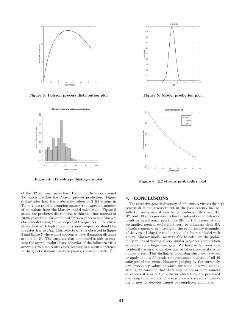
0 10 20 30 40 50 60 7010

−15

10−10

10−5

100

Number of mutations

Pro

ba

bility in

lo

g s

ca

le

Figure 3: Poisson process distribution plot

H2 subtype Hamming distance distribution

Hamming distance

Num

ber

of H

2 se

quen

ce p

airs

0 20 40 60 80 100

020

040

060

080

010

00

Figure 4: H2 subtype histogram plot

of the H2 sequence pairs have Hamming distances around35, which matches the Poisson process prediction. Figure6 illustrates how the probability values of 3 H2 strains inTable 2 are rapidly dropping against the expected numberof mutations from the Markov model calculation. Figure 5shows the predicted distribution within the time interval of70-85 years from the combined Poisson process and Markovchain model using H1 subtype HA1 sequences. The curveshows that with high probability most sequences should bein states H60 to H70. This reflects what is observed in figure2 and figure 7 where most sequences have Hamming distancearound 60-70. This suggests that our model is able to cap-ture the overall evolutionary behavior of the influenza virusaccording to a molecular clock, leading to a natural increasein the genetic distance as time passes, consistent with [1].

0 20 40 60 80 100 120 1400

0.01

0.02

0.03

0.04

0.05

0.06

0.07

0.08

0.09

0.1

States

Pro

ba

bility

H1 with 329 sites

Figure 5: Model prediction plot

0 50 100 150 200 250 300 35010

−250

10−200

10−150

10−100

10−50

100

Number of mutations

Pro

ba

bility in

lo

g s

ca

le

Markov model probability plot

RI−5−

Singapore

RI−5+

Figure 6: H2 strains probability plot

4. CONCLUSIONSThe extensive genetic diversity of influenza A viruses through

genetic drift and reassortment in the past century has re-sulted in many new strains being produced. However, H1,H2, and H3 subtypes strains have displayed cyclic behaviorresulting in influenza pandemics [6]. In the present study,we applied neutral evolution theory to influenza virus HAprotein sequences to investigate the evolutionary dynamicsof the virus. Using the combination of a Poisson model witha novel Markov model, we were able to calculate the proba-bility values of finding a very similar sequence compositionseparated by a large time gap. We have so far been ableto identify several anomalies due to laboratory artifacts orhuman error. This finding is promising since we have yetto apply it in a full scale comprehensive analysis of all 16subtypes of the virus. However, judging by the extremelylow probability values obtained for some observed samplestrains, we conclude that there may be one or more sourcesof various strains of the virus in which they are preservedover long time periods. The existence of reservoirs preserv-ing viruses for decades cannot be completely eliminated.

41

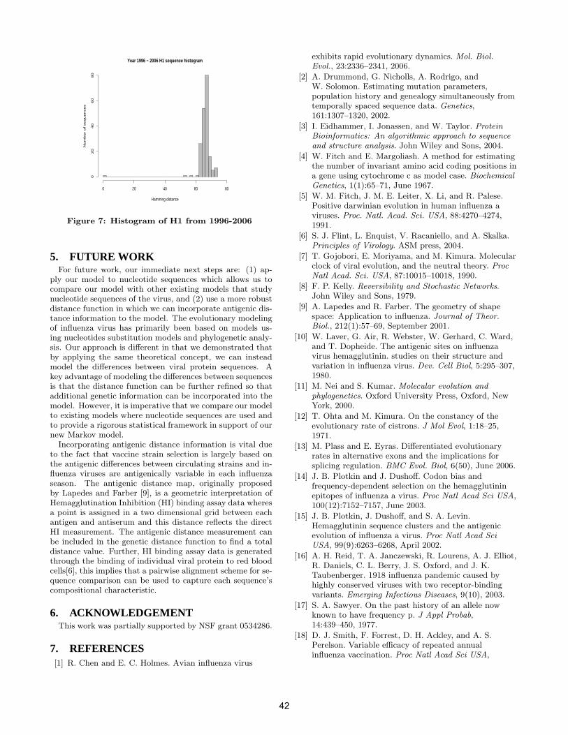
Year 1996 − 2006 H1 sequence histogram

Hamming distance

Nu

mb

er

of

se

qu

en

ce

s

0 20 40 60 80

02

04

06

08

0

Figure 7: Histogram of H1 from 1996-2006

5. FUTURE WORKFor future work, our immediate next steps are: (1) ap-

ply our model to nucleotide sequences which allows us tocompare our model with other existing models that studynucleotide sequences of the virus, and (2) use a more robustdistance function in which we can incorporate antigenic dis-tance information to the model. The evolutionary modelingof influenza virus has primarily been based on models us-ing nucleotides substitution models and phylogenetic analy-sis. Our approach is different in that we demonstrated thatby applying the same theoretical concept, we can insteadmodel the differences between viral protein sequences. Akey advantage of modeling the differences between sequencesis that the distance function can be further refined so thatadditional genetic information can be incorporated into themodel. However, it is imperative that we compare our modelto existing models where nucleotide sequences are used andto provide a rigorous statistical framework in support of ournew Markov model.

Incorporating antigenic distance information is vital dueto the fact that vaccine strain selection is largely based onthe antigenic differences between circulating strains and in-fluenza viruses are antigenically variable in each influenzaseason. The antigenic distance map, originally proposedby Lapedes and Farber [9], is a geometric interpretation ofHemagglutination Inhibition (HI) binding assay data wheresa point is assigned in a two dimensional grid between eachantigen and antiserum and this distance reflects the directHI measurement. The antigenic distance measurement canbe included in the genetic distance function to find a totaldistance value. Further, HI binding assay data is generatedthrough the binding of individual viral protein to red bloodcells[6], this implies that a pairwise alignment scheme for se-quence comparison can be used to capture each sequence’scompositional characteristic.

6. ACKNOWLEDGEMENTThis work was partially supported by NSF grant 0534286.

7. REFERENCES[1] R. Chen and E. C. Holmes. Avian influenza virus

exhibits rapid evolutionary dynamics. Mol. Biol.Evol., 23:2336–2341, 2006.

[2] A. Drummond, G. Nicholls, A. Rodrigo, andW. Solomon. Estimating mutation parameters,population history and genealogy simultaneously fromtemporally spaced sequence data. Genetics,161:1307–1320, 2002.

[3] I. Eidhammer, I. Jonassen, and W. Taylor. ProteinBioinformatics: An algorithmic approach to sequenceand structure analysis. John Wiley and Sons, 2004.

[4] W. Fitch and E. Margoliash. A method for estimatingthe number of invariant amino acid coding positions ina gene using cytochrome c as model case. BiochemicalGenetics, 1(1):65–71, June 1967.

[5] W. M. Fitch, J. M. E. Leiter, X. Li, and R. Palese.Positive darwinian evolution in human influenza aviruses. Proc. Natl. Acad. Sci. USA, 88:4270–4274,1991.

[6] S. J. Flint, L. Enquist, V. Racaniello, and A. Skalka.Principles of Virology. ASM press, 2004.

[7] T. Gojobori, E. Moriyama, and M. Kimura. Molecularclock of viral evolution, and the neutral theory. ProcNatl Acad. Sci. USA, 87:10015–10018, 1990.

[8] F. P. Kelly. Reversibility and Stochastic Networks.John Wiley and Sons, 1979.

[9] A. Lapedes and R. Farber. The geometry of shapespace: Application to influenza. Journal of Theor.Biol., 212(1):57–69, September 2001.

[10] W. Laver, G. Air, R. Webster, W. Gerhard, C. Ward,and T. Dopheide. The antigenic sites on influenzavirus hemagglutinin. studies on their structure andvariation in influenza virus. Dev. Cell Biol, 5:295–307,1980.

[11] M. Nei and S. Kumar. Molecular evolution andphylogenetics. Oxford University Press, Oxford, NewYork, 2000.

[12] T. Ohta and M. Kimura. On the constancy of theevolutionary rate of cistrons. J Mol Evol, 1:18–25,1971.

[13] M. Plass and E. Eyras. Differentiated evolutionaryrates in alternative exons and the implications forsplicing regulation. BMC Evol. Biol, 6(50), June 2006.

[14] J. B. Plotkin and J. Dushoff. Codon bias andfrequency-dependent selection on the hemagglutininepitopes of influenza a virus. Proc Natl Acad Sci USA,100(12):7152–7157, June 2003.

[15] J. B. Plotkin, J. Dushoff, and S. A. Levin.Hemagglutinin sequence clusters and the antigenicevolution of influenza a virus. Proc Natl Acad SciUSA, 99(9):6263–6268, April 2002.

[16] A. H. Reid, T. A. Janczewski, R. Lourens, A. J. Elliot,R. Daniels, C. L. Berry, J. S. Oxford, and J. K.Taubenberger. 1918 influenza pandemic caused byhighly conserved viruses with two receptor-bindingvariants. Emerging Infectious Diseases, 9(10), 2003.

[17] S. A. Sawyer. On the past history of an allele nowknown to have frequency p. J Appl Probab,14:439–450, 1977.

[18] D. J. Smith, F. Forrest, D. H. Ackley, and A. S.Perelson. Variable efficacy of repeated annualinfluenza vaccination. Proc Natl Acad Sci USA,

42

96(24):14001–14006, November 1999.

[19] Y. Suzuki and M. Nei. Origin and evolution ofinfluenza virus hemagglutinin genes. Mol. Biol. Evol.,19(4):501–509, 2002.

[20] R. Webster, W. Bean, O. Gorman, T. Chambers, andY. Kawaoka. Evolution and ecology of influenza aviruses. Microbiological Reviews, pages 152–179,March 1992.

[21] WHO. Epidemic and pandemic alert and response(epr):international response to the distribution of ah2n2 influenza virus for laboratory testing: Riskconsidered low for laboratory workers and the public.April 2005.

[22] M. Worobey. Phylogenetic evidence againstevolutionary stasis and natural abiotic reservoirs ofinfluenza a virus. J of Virology, 82(7):3769–3774, April2008.

[23] P. B. Y. Bao, D. Dernovoy, B. Kiryutin, L. Zaslavsky,T. Tatusova, J. Ostell, and D. Lipman. The influenzavirus resource at the national center for biotechnologyinformation. Journal of Virology, 82(2):596–601,January 2008.

[24] S. Yoshiyuki. Natural selection on the influenza virusgenome. Mol. Biol. Evol, 23, June 2006.

[25] E. Zuckerkandl and L. Pauling. Molecular disease,evolution, and genetic heterogeneity. Academic Press,New York, 1962.

43

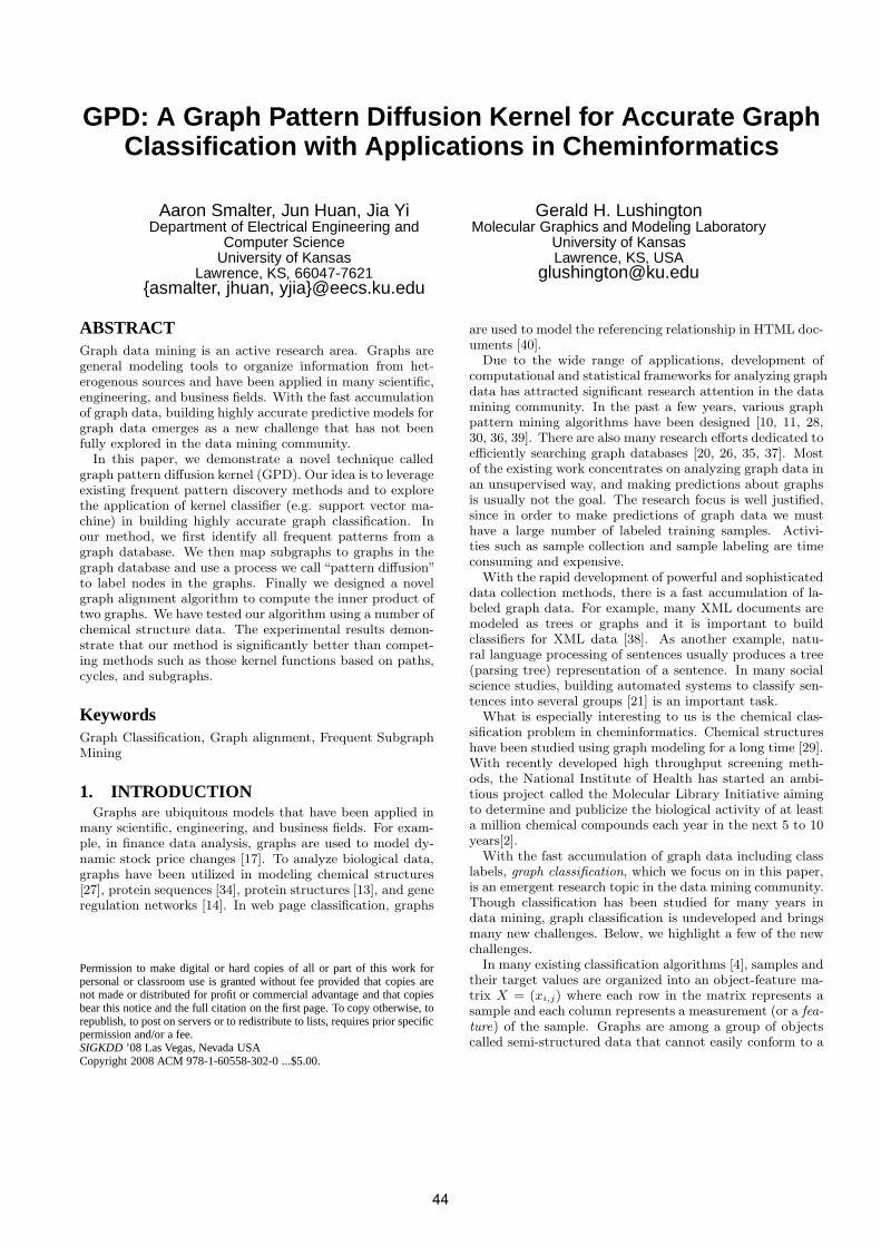
GPD: A Graph Pattern Diffusion Kernel for Accurate GraphClassification with Applications in Cheminformatics

Aaron Smalter, Jun Huan, Jia YiDepartment of Electrical Engineering and

Computer ScienceUniversity of Kansas

Lawrence, KS, 66047-7621{asmalter, jhuan, yjia}@eecs.ku.edu

Gerald H. LushingtonMolecular Graphics and Modeling Laboratory

University of KansasLawrence, KS, USA

glushington@ku.edu

ABSTRACTGraph data mining is an active research area. Graphs aregeneral modeling tools to organize information from het-erogenous sources and have been applied in many scientific,engineering, and business fields. With the fast accumulationof graph data, building highly accurate predictive models forgraph data emerges as a new challenge that has not beenfully explored in the data mining community.

In this paper, we demonstrate a novel technique calledgraph pattern diffusion kernel (GPD). Our idea is to leverageexisting frequent pattern discovery methods and to explorethe application of kernel classifier (e.g. support vector ma-chine) in building highly accurate graph classification. Inour method, we first identify all frequent patterns from agraph database. We then map subgraphs to graphs in thegraph database and use a process we call “pattern diffusion”to label nodes in the graphs. Finally we designed a novelgraph alignment algorithm to compute the inner product oftwo graphs. We have tested our algorithm using a number ofchemical structure data. The experimental results demon-strate that our method is significantly better than compet-ing methods such as those kernel functions based on paths,cycles, and subgraphs.

KeywordsGraph Classification, Graph alignment, Frequent SubgraphMining

1. INTRODUCTIONGraphs are ubiquitous models that have been applied in

many scientific, engineering, and business fields. For exam-ple, in finance data analysis, graphs are used to model dy-namic stock price changes [17]. To analyze biological data,graphs have been utilized in modeling chemical structures[27], protein sequences [34], protein structures [13], and generegulation networks [14]. In web page classification, graphs

Permission to make digital or hard copies of all or part of this work forpersonal or classroom use is granted without fee provided that copies arenot made or distributed for profit or commercial advantage and that copiesbear this notice and the full citation on the first page. To copy otherwise, torepublish, to post on servers or to redistribute to lists, requires prior specificpermission and/or a fee.SIGKDD ’08 Las Vegas, Nevada USACopyright 2008 ACM 978-1-60558-302-0 ...$5.00.

are used to model the referencing relationship in HTML doc-uments [40].

Due to the wide range of applications, development ofcomputational and statistical frameworks for analyzing graphdata has attracted significant research attention in the datamining community. In the past a few years, various graphpattern mining algorithms have been designed [10, 11, 28,30, 36, 39]. There are also many research efforts dedicated toefficiently searching graph databases [20, 26, 35, 37]. Mostof the existing work concentrates on analyzing graph data inan unsupervised way, and making predictions about graphsis usually not the goal. The research focus is well justified,since in order to make predictions of graph data we musthave a large number of labeled training samples. Activi-ties such as sample collection and sample labeling are timeconsuming and expensive.

With the rapid development of powerful and sophisticateddata collection methods, there is a fast accumulation of la-beled graph data. For example, many XML documents aremodeled as trees or graphs and it is important to buildclassifiers for XML data [38]. As another example, natu-ral language processing of sentences usually produces a tree(parsing tree) representation of a sentence. In many socialscience studies, building automated systems to classify sen-tences into several groups [21] is an important task.

What is especially interesting to us is the chemical clas-sification problem in cheminformatics. Chemical structureshave been studied using graph modeling for a long time [29].With recently developed high throughput screening meth-ods, the National Institute of Health has started an ambi-tious project called the Molecular Library Initiative aimingto determine and publicize the biological activity of at leasta million chemical compounds each year in the next 5 to 10years[2].

With the fast accumulation of graph data including classlabels, graph classification, which we focus on in this paper,is an emergent research topic in the data mining community.Though classification has been studied for many years indata mining, graph classification is undeveloped and bringsmany new challenges. Below, we highlight a few of the newchallenges.

In many existing classification algorithms [4], samples andtheir target values are organized into an object-feature ma-trix X = (xi,j) where each row in the matrix represents asample and each column represents a measurement (or a fea-ture) of the sample. Graphs are among a group of objectscalled semi-structured data that cannot easily conform to a

44

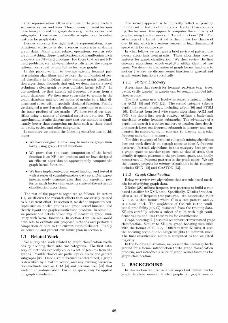
matrix representation. Other examples in the group includesequences, cycles, and trees. Though many different featureshave been proposed for graph data (e.g. paths, cycles, andsubgraphs), there is no universally accepted way to definefeatures for graph data.

Besides choosing the right feature representation, com-putational efficiency is also a serious concern in analyzinggraph data. Many graph related operations, such as sub-graph matching, clique identification, and hamiltonian cyclediscovery are NP-hard problems. For those that are not NP-hard problems, e.g. all-by-all shortest distance, the compu-tational cost could be prohibitive for large graphs.

In this paper, we aim to leverage existing frequent pat-tern mining algorithms and explore the application of ker-nel classifiers in building highly accurate graph classifica-tion algorithms. Towards that end, we demonstrate a noveltechnique called graph pattern diffusion kernel (GPD). Inour method, we first identify all frequent patterns from agraph database. We then map subgraphs to graphs in thegraph database and project nodes of graphs to a high di-mensional space with a specially designed function. Finallywe designed a novel graph alignment algorithm to computethe inner product of two graphs. We have tested our algo-rithm using a number of chemical structure data sets. Theexperimental results demonstrate that our method is signif-icantly better than competing methods such as those basedon paths, cycles, and other subgraphs.

In summary we present the following contributions in thispaper:

• We have designed a novel way to measure graph simi-larity using graph kernel functions

• We prove that the exact computation of the kernelfunction is an NP-hard problem and we have designedan efficient algorithm to approximately compute thegraph kernel function.

• We have implemented our kernel function and tested itwith a series of cheminformatics data sets. Our exper-imental study demonstrates that our algorithm per-forms much better than existing state-of-the-art graphclassification algorithms.

The rest of the paper is organized as follows. In section1.1, we discuss the research efforts that are closely relatedto our current effort. In section 2, we define important con-cepts such as labeled graphs and graph kernel function, andclearly layout the graph classification problem. In section 3,we present the details of our way of measuring graph simi-larity with kernel functions. In section 4 we use real-worlddata sets to evaluate our proposed methods and perform acomparison of ours to the current state-of-the-art. Finallywe conclude and present our future plan in section 5.

1.1 Related WorkWe survey the work related to graph classification meth-

ods by dividing them into two categories. The first cate-gory of methods explicitly collect a set of features from thegraphs. Possible choices are paths, cycles, trees, and generalsubgraphs [38]. Once a set of features is determined, a graphis described by a feature vector, and any existing classifica-tion methods such as CBA [4] and decision tree [24] thatwork in an n-dimensional Euclidian space, may be appliedfor graph classification.

The second approach is to implicitly collect a (possiblyinfinite) set of features from graphs. Rather than comput-ing the features, this approach computes the similarity ofgraphs, using the framework of “kernel functions” [31]. Theadvantage of a kernel method is that it has low chance ofover fitting, which is a serious concern in high dimensionalspace with low sample size.

In what follows we first give a brief review of pattern dis-covery algorithms from graphs. Those algorithms providefeatures for graph classification. We then review the firstcategory algorithms, which explicitly utilize identified fea-tures. We delay the discussion of graph kernel functions tosection 2 where we discuss kernel function in general andgraph kernel functions specifically.

1.1.1 Pattern DiscoveryAlgorithms that search for frequent patterns (e.g. trees,

paths, cyclic graphs) in graphs can be roughly divided intothree groups.

The first group uses a level-wise search strategy, includ-ing AGM [15] and FSG [22]. The second category takes adepth-first search strategy, including gSpan[36] and FFSM[16]. Different from level-wise search algorithms AGM andFSG, the depth-first search strategy utilizes a back-trackalgorithm to mine frequent subgraphs. The advantage of adepth-first search is a better memory utilization since depth-first search keeps one frequent subgraph in memory and enu-merates its supergraphs, in contrast to keeping all k-edgefrequent subgraph in memory.

The third category of frequent subgraph mining algorithmsdoes not work directly on a graph space to identify frequentpatterns. Instead, algorithms in this category first projecta graph space to another space such as that of trees, thenidentify frequent patterns in the projected space, and finallyreconstruct all frequent patterns in the graph space. We callthis strategy progressive mining. Algorithms in this categoryincludes SPIN [12] and GASTON [23].

1.1.2 Graph ClassificationBelow we review two algorithms that use rule based meth-

ods for classifying graph data.XRules [38] utilizes frequent tree-patterns to build a rule

based classifier for XML data. Specifically, XRules first iden-tifies a set of frequent tree-patterns. An association rule:G → ci is then formed where G is a tree pattern and ci

is a class label. The confidence of the rule is the condi-tional probability p(ci|G) estimated from the training data.XRules carefully selects a subset of rules with high confi-dence values and uses those rules for classification.

Graph boosting [21] also utilizes substructures toward graphclassification. Similar to XRules, graph boosting uses ruleswith the format of G → ci. Different from XRules, it usesthe boosting technique to assign weights to different rules.The final classification result is computed as the weightedmajority.

In the following discussion, we present the necessary back-ground for a formal introduction to the graph classificationproblem, and introduce a suite of graph kernel functions forgraph classification.

2. BACKGROUNDIn this section we discuss a few important definitions for

graph database mining: labeled graphs, subgraph isomor-

45

(1) Graph P

a b

b

b

x

y

y

x

y

p1

p3

p2

p4

a

b

b

x

y

q2

q1

q3

(2) Graph Q

b

b

b

y

y

ys2

s3

s1

(3) Graph S

Figure 1: A Database of three labeled graphs.

phic relation, graph kernel function, and graph classifica-tion.

Definition 2.1. A labeled graph G is a quadruple G =(V, E, Σ, λ) where V is a set of vertices or nodes and E ⊆V × V is a set of undirected edges. Σ is a set of (disjoint)vertex and edge labels, and λ: V ∪E → Σ is a function thatassigns labels to vertices and edges. We assume that a totalordering is defined on the labels in Σ.

A graph database is a set of labeled graphs.

Definition 2.2. A graph G′ = (V ′, E′, Σ′, λ′) is sub-

graph isomorphic to G = (V, E,Σ, λ), denoted by G′ ⊆ G,if there exists a 1-1 mapping f : V ′ → V such that

• ∀v ∈ V ′, λ′(v) = λ(f(v))

• ∀(u, v) ∈ E′, (f(u), f(v)) ∈ E, and

• ∀(u, v) ∈ E′, λ′(u, v) = λ(f(u), f(v))

.

The function f is a subgraph isomorphism from graph G′

to graph G. We say G′ occurs in G if G′ ⊆ G. Given a sub-graph isomorphism f , the image of the domain V ′ (f(V ′))is an embedding of G′ in G.

Example 2.1. Figure 1 shows a graph database of threelabeled graphs. The mapping (isomorphism) q1 → p3, q2 →p1, and q3 → p2 demonstrates that graph Q is subgraph iso-morphic to P and hence Q occurs in P . Set {p1, p2, p3} isan embedding of Q in P . Similarly, graph S occurs in graphP but not Q.

Problem Statement: Given a graph space G∗, a setof n graphs sampled from G∗ and the related target valuesof these graphs D = {(Gi, Ti, )}

ni=1, the graph classifica-

tion problem is to estimate a function F : G∗ → T thataccurately map graphs to their target value.

By classification we assume all target values are discretevalues, otherwise it is a regression problem. Below, we re-view several algorithms for graph classification that workwithin a common framework called a kernel function. Theterm kernel function refers to an operation of computing theinner product between two points in a Hilbert space. Kernelfunctions are widely used in classification of data in a highdimensional feature space.

2.1 Kernel Functions for GraphsGraph kernel functions are simply kernel functions that

have been defined to compute the inner product between twographs. In recent years a variety of graph kernel functions

have been developed, with promising application results asdescribed by Ralaviola et al. [25]. Among these methods,some kernel functions draw on graph features such as walks[19] or cycles [9], while others may use different approachessuch as genetic algorithms [3], frequent subgraphs [6], orgraph alignment [7]. We review two graph kernel functionsin details due to their close relationship to our algorithm.

Kashima et al. [19] proposed a kernel function called themarginalized graph kernel. This kernel function is basedon the use of shared label sequences in the comparison ofgraphs. Their marginalized graph kernel uses a Markovmodel to randomly generate walks of a labeled graph, basedon a transition probability matrix combined with a walk ter-mination probability. These collections of random walks arethen compared and the number of shared sequences is usedto determine the overall similarity between two graphs.

The optimal assignment kernel, proposed by Frohlich etal. [7], differs significantly from the marginalized graph ker-nel in that it attempts to align two graphs, rather than com-pare sets of linear substructures. This kernel function firstcomputes the similarity between all vertices in one graph andthose in another. The similarity between the two graphs isthen computed by finding the maximal weighted bipartitegraph between the two sets of vertices, called the optimalassignment. The authors investigate an extension of thismethod whereby certain structure patterns defined a prioriby expert knowledge, are collapsed into single vertices, andthis reduced graph is used as input to the optimal assign-ment kernel.

3. GRAPH ALIGNMENT KERNELSHere we present our design of a pattern diffusion kernel.

We start the section by first presenting a general framework.We prove, through a reduction to the subgraph isomorphismproblem, that the computational cost of the general frame-work can be prohibitive for large graphs. We then presentour pattern based graph alignment kernel. Finally we showa technique we call “pattern diffusion” that can significantlyimprove graph classification accuracy in practice.

3.1 Graph Similarity Measurement with Align-ment

An alignment of two graphs G and G′ (assuming |V [G]| ≤|V [G′]|) is a 1-1 mapping π : V [G] → V [G′]. Given analignment π, we define the similarity between two graphs,as measured by a kernel function kA, below:

kA(G, G′) = max

π

X

v

kn(v, π(v)) +X

u,v

ke((u, v), (π(u), π(v)))

(1)The function kn is a kernel function to measure the simi-

larity of node labels and the function ke is a kernel functionto measure the similarity of edge labels. Equation 1 usesan additive model to compute the similarity between twographs. The maximal similarity among all possible map-pings is defined as the similarity between two graphs.

3.2 NP-hardness of Graph Alignment KernelFunction

It is no surprise that computing the graph alignment ker-nel is an NP-hard problem. We prove this with a reductionfrom the graph alignment kernel to the subgraph isomor-

46

phism problem. In the following paragraphs, we assume wehave an efficient solver of the graph alignment kernel prob-lem, we show that the same solver can be used to solve thesubgraph isomorphism problem efficiently. Since the sub-graph isomorphism problem is an NP-hard problem, withthe reduction we mentioned before we prove that the graphalignment kernel problem is therefore an NP-hard problemas well. Note: this subsection is a stand-alone component ofour paper, and readers who choose to skip this section shouldencounter no difficulty in reading the rest of the paper.

Given two graphs G and G′ (for simplicity, assume nodesand edges in G and G′ are not labeled as usually studied inthe subgraph isomorphism problem), we use a node kernelfunction that returns a constant 0. We define an edge kernelfunction ke : V [G] × V [G] × V [G′] × V [G′] → R as

ke((u, v), (u′, v

′)) =

1 if (u, v) ∈ E[G] and (u′, v′) ∈ E[G′]0 otherwise

With the constant node function and the specialized edgefunction, the kernel function of two graphs is simplified tothe following format:

kA(G, G′) = max

π

X

u,v

ke((u, v), (π(u), π(v))) (2)

We establish the NP-hardness of the graph alignment ker-nel with the following theorem.

Theorem 3.1. Given two (unlabeled) graphs G and G′

and the edge kernel function ke defined previously, G is sub-graph isomorphic to G′ if and only if Ka(G, G′) = |E[G]|

Proof. If: We notice from the definition of ke that themaximal value of Ka(G, G′) is |E[G]|. Given Ka(G, G′) =|E[G]|, we claim that there exists an alignment functionπ : V [G] → V [G′] such that for all (u, v) ∈ E[G] we have(π(u), π(v)) ∈ E[G′]. The existence of such a function π

guarantees that graph G is a subgraph of G′.

Only if: Given G is a subgraph of G′, we have an align-ment function π : V [G] → V [G′] such that for all (u, v) ∈E[G] we have (π(u), π(v)) ∈ E[G′]. According to Equation2, Ka(G, G′) = |E[G]|.

Theorem 3.1 shows that the graph alignment kernel prob-lem is no easier than the subgraph isomorphism problemand hence is at least NP-hard in complexity.

3.3 Graph Node Alignment KernelTo derive an efficient algorithm scalable to large graphs,

our idea is that we use a function f to map nodes in a graphto a high (possibly infinite) dimensional feature space thatcaptures not only the node label information but also theneighborhood topological information around the node. Ifwe have such function f , we may simplify the graph kernelfunction with the following formula:

kM (G, G′) = max

π

X

v∈V [G]

kn(f(v), f(π(v))) (3)

Where π : V [G] → V [G′] denotes an alignment of graphG and G′. f(v) is a set of “features” associated with a node.

With this modification, the optimization problem thatsearches for the best alignment can be solved in polyno-mial time. To derive a polynomial running time algorithm,

we construct a weighted complete bipartite graph by mak-ing every node pair (u,v) ∈ V [G] × V [G′] incident on anedge. The weight of the edge (u,v) is kn(f(v), f(u)). InFigure 2, we show a weighted complete bipartite graph forV [G] = {v1, v2, v3} and V [G′] = {u1, u2, u3}.

With the bipartite graph, a search for the best alignmentbecomes a search for the maximum weighted bipartite sub-graph from the complete bipartite graph. Many networkflow based algorithms (e.g. linear programming) can be usedto obtain the maximum weighted bipartite subgraph. Weuse the Hungarian algorithm with complexity O(|V [G]|3).For details of the Hungarian algorithm see [1].

Kn(v2,u1)

v1

v2

v3

u1

u2

u3

Kn(v1,u2)

Kn(v3,u3)

Figure 2: The maximum weighted bipartite graph

for graph alignment. Highlighted edges (v1, u2), (v2, u1),

(v3, u3) have larger weights than the rest of the edges

(dashed).

Applying the Hungarian algorithm to graph alignmentwas first explored by [7] for chemical compound classifica-tion. In contrast to their algorithm, which utilized domainknowledge of chemical compounds extensively and devel-oped a complicated recursive function to compute the sim-ilarity between nodes, we develop a new framework thatmaps such nodes to a high dimensional space in order tomeasure the similarity between two nodes without assum-ing any domain knowledge. Even in cheminformatics, ourexperiments shows that our technique generate similar andsometimes better classification accuracies compared to themethod reported in [7].

Unfortunately, using the Hungarian algorithm for assign-ment, as used by [7] is not a true Mercer kernel. Since ourproposed kernel function uses this algorithm as well, it is alsonot a Mercer kernel. Like in [7], however, we have found thatpractically our kernel still performs competitively.

3.4 Pattern DiffusionIn this section, we introduce a novel function “pattern

diffusion” to project nodes in a graph to a high dimensionalspace that captures both node labeling information and localtopology information. Our design has the following advan-tages as a kernel function:

• Our design is generic and does not assume any domainknowledge from a specific application. The diffusionprocess may be applied to graphs with dramaticallydifferent characteristics.

• The diffusion process is straightforward to implementand can be computed efficiently.

• We prove that the diffusion process is related to theprobability distribution of a graph random walk (in

47

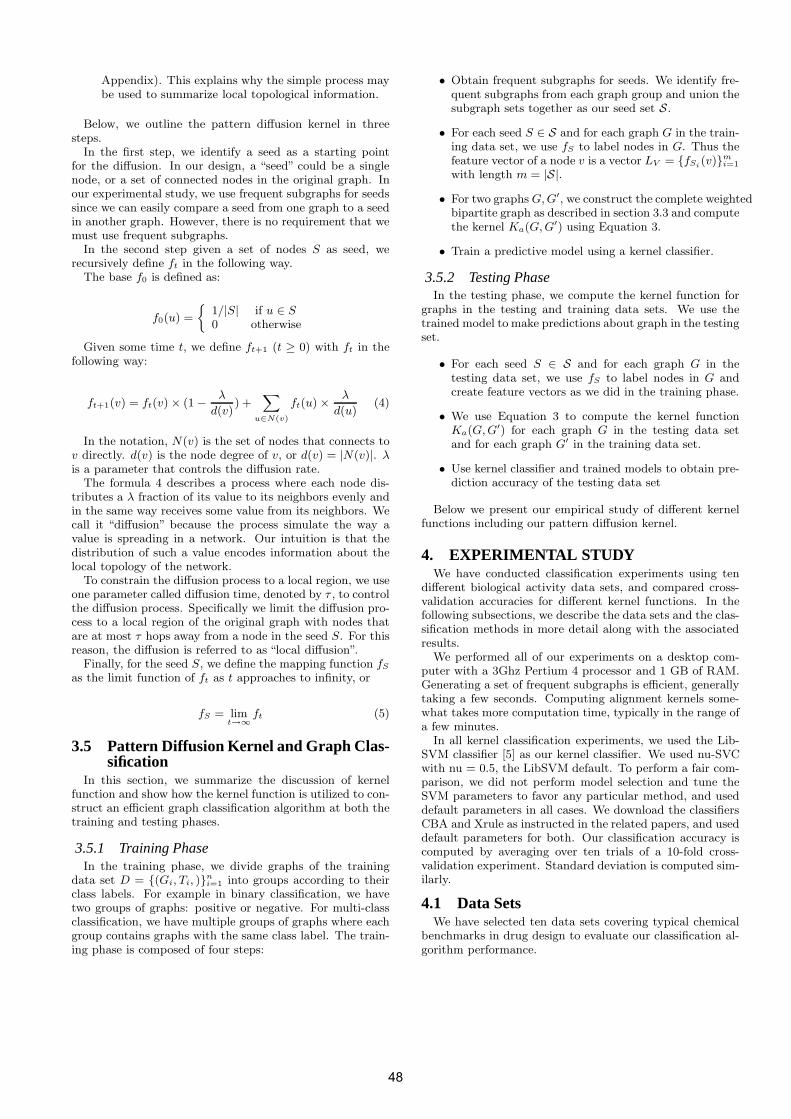
Appendix). This explains why the simple process maybe used to summarize local topological information.

Below, we outline the pattern diffusion kernel in threesteps.

In the first step, we identify a seed as a starting pointfor the diffusion. In our design, a “seed” could be a singlenode, or a set of connected nodes in the original graph. Inour experimental study, we use frequent subgraphs for seedssince we can easily compare a seed from one graph to a seedin another graph. However, there is no requirement that wemust use frequent subgraphs.

In the second step given a set of nodes S as seed, werecursively define ft in the following way.

The base f0 is defined as:

f0(u) =

1/|S| if u ∈ S

0 otherwise

Given some time t, we define ft+1 (t ≥ 0) with ft in thefollowing way:

ft+1(v) = ft(v) × (1 −λ

d(v)) +

X

u∈N(v)

ft(u) ×λ

d(u)(4)

In the notation, N(v) is the set of nodes that connects tov directly. d(v) is the node degree of v, or d(v) = |N(v)|. λ

is a parameter that controls the diffusion rate.The formula 4 describes a process where each node dis-

tributes a λ fraction of its value to its neighbors evenly andin the same way receives some value from its neighbors. Wecall it “diffusion” because the process simulate the way avalue is spreading in a network. Our intuition is that thedistribution of such a value encodes information about thelocal topology of the network.

To constrain the diffusion process to a local region, we useone parameter called diffusion time, denoted by τ , to controlthe diffusion process. Specifically we limit the diffusion pro-cess to a local region of the original graph with nodes thatare at most τ hops away from a node in the seed S. For thisreason, the diffusion is referred to as “local diffusion”.

Finally, for the seed S, we define the mapping function fS

as the limit function of ft as t approaches to infinity, or

fS = limt→∞

ft (5)

3.5 Pattern Diffusion Kernel and Graph Clas-sification

In this section, we summarize the discussion of kernelfunction and show how the kernel function is utilized to con-struct an efficient graph classification algorithm at both thetraining and testing phases.

3.5.1 Training PhaseIn the training phase, we divide graphs of the training

data set D = {(Gi, Ti, )}ni=1 into groups according to their

class labels. For example in binary classification, we havetwo groups of graphs: positive or negative. For multi-classclassification, we have multiple groups of graphs where eachgroup contains graphs with the same class label. The train-ing phase is composed of four steps:

• Obtain frequent subgraphs for seeds. We identify fre-quent subgraphs from each graph group and union thesubgraph sets together as our seed set S .

• For each seed S ∈ S and for each graph G in the train-ing data set, we use fS to label nodes in G. Thus thefeature vector of a node v is a vector LV = {fSi

(v)}mi=1

with length m = |S|.

• For two graphs G, G′, we construct the complete weightedbipartite graph as described in section 3.3 and computethe kernel Ka(G, G′) using Equation 3.

• Train a predictive model using a kernel classifier.

3.5.2 Testing PhaseIn the testing phase, we compute the kernel function for

graphs in the testing and training data sets. We use thetrained model to make predictions about graph in the testingset.

• For each seed S ∈ S and for each graph G in thetesting data set, we use fS to label nodes in G andcreate feature vectors as we did in the training phase.

• We use Equation 3 to compute the kernel functionKa(G, G′) for each graph G in the testing data setand for each graph G′ in the training data set.

• Use kernel classifier and trained models to obtain pre-diction accuracy of the testing data set

Below we present our empirical study of different kernelfunctions including our pattern diffusion kernel.

4. EXPERIMENTAL STUDYWe have conducted classification experiments using ten

different biological activity data sets, and compared cross-validation accuracies for different kernel functions. In thefollowing subsections, we describe the data sets and the clas-sification methods in more detail along with the associatedresults.

We performed all of our experiments on a desktop com-puter with a 3Ghz Pertium 4 processor and 1 GB of RAM.Generating a set of frequent subgraphs is efficient, generallytaking a few seconds. Computing alignment kernels some-what takes more computation time, typically in the range ofa few minutes.

In all kernel classification experiments, we used the Lib-SVM classifier [5] as our kernel classifier. We used nu-SVCwith nu = 0.5, the LibSVM default. To perform a fair com-parison, we did not perform model selection and tune theSVM parameters to favor any particular method, and useddefault parameters in all cases. We download the classifiersCBA and Xrule as instructed in the related papers, and useddefault parameters for both. Our classification accuracy iscomputed by averaging over ten trials of a 10-fold cross-validation experiment. Standard deviation is computed sim-ilarly.

4.1 Data SetsWe have selected ten data sets covering typical chemical

benchmarks in drug design to evaluate our classification al-gorithm performance.

48

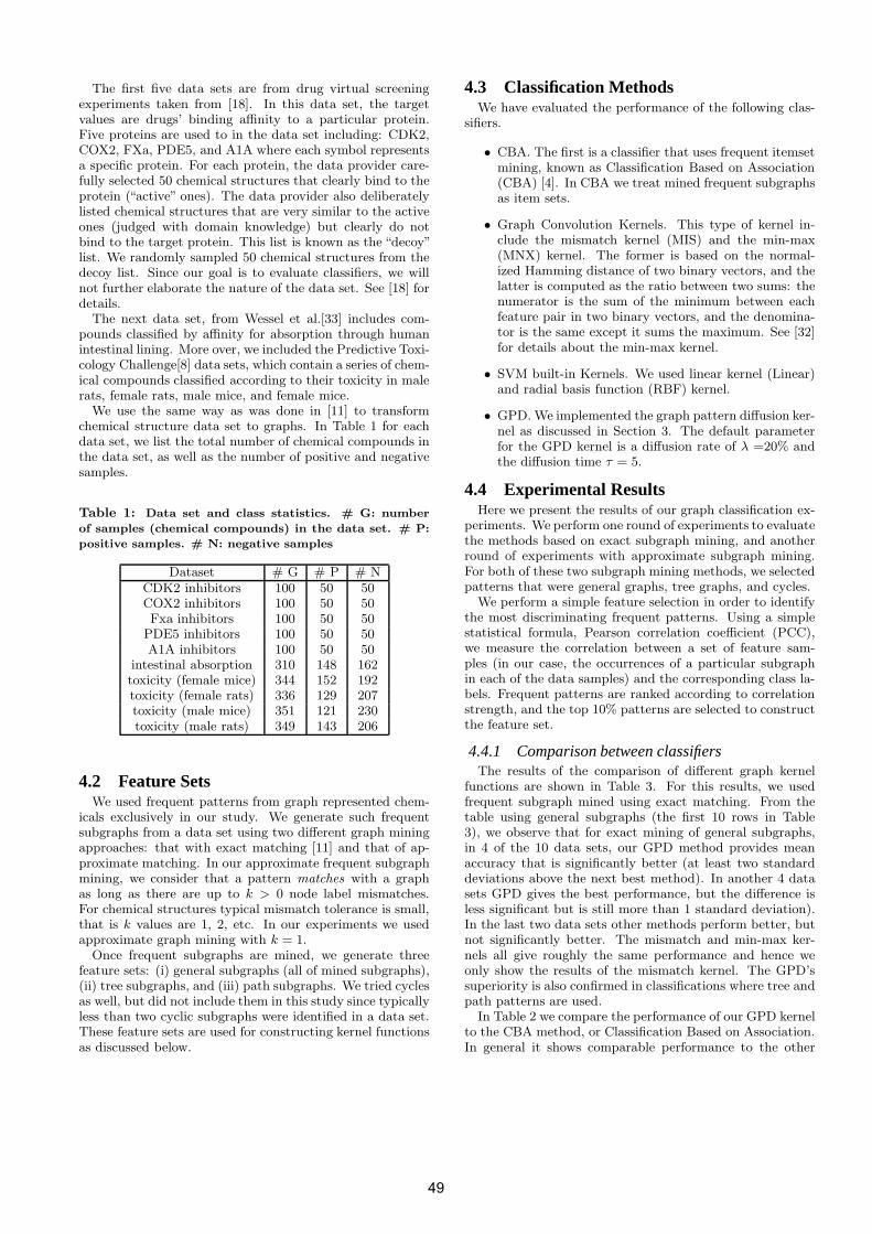
The first five data sets are from drug virtual screeningexperiments taken from [18]. In this data set, the targetvalues are drugs’ binding affinity to a particular protein.Five proteins are used to in the data set including: CDK2,COX2, FXa, PDE5, and A1A where each symbol representsa specific protein. For each protein, the data provider care-fully selected 50 chemical structures that clearly bind to theprotein (“active” ones). The data provider also deliberatelylisted chemical structures that are very similar to the activeones (judged with domain knowledge) but clearly do notbind to the target protein. This list is known as the “decoy”list. We randomly sampled 50 chemical structures from thedecoy list. Since our goal is to evaluate classifiers, we willnot further elaborate the nature of the data set. See [18] fordetails.

The next data set, from Wessel et al.[33] includes com-pounds classified by affinity for absorption through humanintestinal lining. More over, we included the Predictive Toxi-cology Challenge[8] data sets, which contain a series of chem-ical compounds classified according to their toxicity in malerats, female rats, male mice, and female mice.

We use the same way as was done in [11] to transformchemical structure data set to graphs. In Table 1 for eachdata set, we list the total number of chemical compounds inthe data set, as well as the number of positive and negativesamples.

Table 1: Data set and class statistics. # G: number

of samples (chemical compounds) in the data set. # P:

positive samples. # N: negative samples

Dataset # G # P # NCDK2 inhibitors 100 50 50COX2 inhibitors 100 50 50Fxa inhibitors 100 50 50

PDE5 inhibitors 100 50 50A1A inhibitors 100 50 50

intestinal absorption 310 148 162toxicity (female mice) 344 152 192toxicity (female rats) 336 129 207toxicity (male mice) 351 121 230toxicity (male rats) 349 143 206

4.2 Feature SetsWe used frequent patterns from graph represented chem-

icals exclusively in our study. We generate such frequentsubgraphs from a data set using two different graph miningapproaches: that with exact matching [11] and that of ap-proximate matching. In our approximate frequent subgraphmining, we consider that a pattern matches with a graphas long as there are up to k > 0 node label mismatches.For chemical structures typical mismatch tolerance is small,that is k values are 1, 2, etc. In our experiments we usedapproximate graph mining with k = 1.

Once frequent subgraphs are mined, we generate threefeature sets: (i) general subgraphs (all of mined subgraphs),(ii) tree subgraphs, and (iii) path subgraphs. We tried cyclesas well, but did not include them in this study since typicallyless than two cyclic subgraphs were identified in a data set.These feature sets are used for constructing kernel functionsas discussed below.

4.3 Classification MethodsWe have evaluated the performance of the following clas-

sifiers.

• CBA. The first is a classifier that uses frequent itemsetmining, known as Classification Based on Association(CBA) [4]. In CBA we treat mined frequent subgraphsas item sets.

• Graph Convolution Kernels. This type of kernel in-clude the mismatch kernel (MIS) and the min-max(MNX) kernel. The former is based on the normal-ized Hamming distance of two binary vectors, and thelatter is computed as the ratio between two sums: thenumerator is the sum of the minimum between eachfeature pair in two binary vectors, and the denomina-tor is the same except it sums the maximum. See [32]for details about the min-max kernel.

• SVM built-in Kernels. We used linear kernel (Linear)and radial basis function (RBF) kernel.

• GPD. We implemented the graph pattern diffusion ker-nel as discussed in Section 3. The default parameterfor the GPD kernel is a diffusion rate of λ =20% andthe diffusion time τ = 5.

4.4 Experimental ResultsHere we present the results of our graph classification ex-

periments. We perform one round of experiments to evaluatethe methods based on exact subgraph mining, and anotherround of experiments with approximate subgraph mining.For both of these two subgraph mining methods, we selectedpatterns that were general graphs, tree graphs, and cycles.

We perform a simple feature selection in order to identifythe most discriminating frequent patterns. Using a simplestatistical formula, Pearson correlation coefficient (PCC),we measure the correlation between a set of feature sam-ples (in our case, the occurrences of a particular subgraphin each of the data samples) and the corresponding class la-bels. Frequent patterns are ranked according to correlationstrength, and the top 10% patterns are selected to constructthe feature set.

4.4.1 Comparison between classifiersThe results of the comparison of different graph kernel

functions are shown in Table 3. For this results, we usedfrequent subgraph mined using exact matching. From thetable using general subgraphs (the first 10 rows in Table3), we observe that for exact mining of general subgraphs,in 4 of the 10 data sets, our GPD method provides meanaccuracy that is significantly better (at least two standarddeviations above the next best method). In another 4 datasets GPD gives the best performance, but the difference isless significant but is still more than 1 standard deviation).In the last two data sets other methods perform better, butnot significantly better. The mismatch and min-max ker-nels all give roughly the same performance and hence weonly show the results of the mismatch kernel. The GPD’ssuperiority is also confirmed in classifications where tree andpath patterns are used.

In Table 2 we compare the performance of our GPD kernelto the CBA method, or Classification Based on Association.In general it shows comparable performance to the other

49

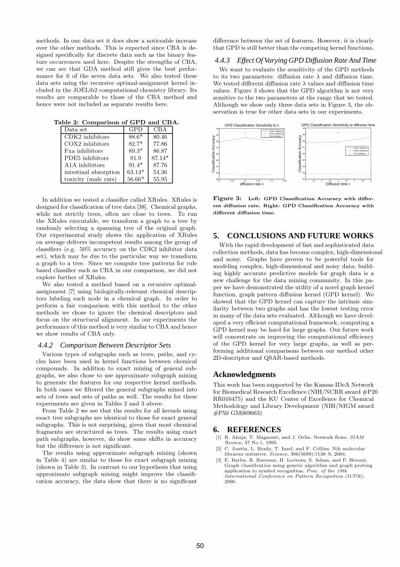
methods. In one data set it does show a noticeable increaseover the other methods. This is expected since CBA is de-signed specifically for discrete data such as the binary fea-ture occurrences used here. Despite the strengths of CBA,we can see that GDA method still gives the best perfor-mance for 6 of the seven data sets. We also tested thesedata sets using the recursive optimal-assignment kernel in-cluded in the JOELib2 computational chemistry library. Itsresults are comparable to those of the CBA method andhence were not included as separate results here.

Table 2: Comparison of GPD and CBA.Data set GPD CBACDK2 inhibitors 88.6* 80.46COX2 inhibitors 82.7* 77.86Fxa inhibitors 89.3* 86.87PDE5 inhibitors 81.9 87.14*A1A inhibitors 91.4* 87.76intestinal absorption 63.14* 54.36toxicity (male rats) 56.66* 55.95

In addition we tested a classifier called XRules. XRules isdesigned for classification of tree data [38]. Chemical graphs,while not strictly trees, often are close to trees. To runthe XRules executable, we transform a graph to a tree byrandomly selecting a spanning tree of the original graph.Our experimental study shows the application of XRuleson average delivers incompetent results among the group ofclassifiers (e.g. 50% accuracy on the CDK2 inhibitor dataset), which may be due to the particular way we transforma graph to a tree. Since we compute tree patterns for rulebased classifier such as CBA in our comparison, we did notexplore further of XRules.

We also tested a method based on a recursive optimal-assignment [7] using biologically-relevant chemical descrip-tors labeling each node in a chemical graph. In order toperform a fair comparison with this method to the othermethods we chose to ignore the chemical descriptors andfocus on the structural alignment. In our experiments theperformance of this method is very similar to CBA and hencewe show results of CBA only.

4.4.2 Comparison Between Descriptor SetsVarious types of subgraphs such as trees, paths, and cy-

cles have been used in kernel functions between chemicalcompounds. In addition to exact mining of general sub-graphs, we also chose to use approximate subgraph miningto generate the features for our respective kernel methods.In both cases we filtered the general subgraphs mined intosets of trees and sets of paths as well. The results for theseexperiments are given in Tables 2 and 3 above.

From Table 2 we see that the results for all kernels usingexact tree subgraphs are identical to those for exact generalsubgraphs. This is not surprising, given that most chemicalfragments are structured as trees. The results using exactpath subgraphs, however, do show some shifts in accuracybut the difference is not significant.

The results using approximate subgraph mining (shownin Table 4) are similar to those for exact subgraph mining(shown in Table 3). In contrast to our hypothesis that usingapproximate subgraph mining might improve the classifi-cation accuracy, the data show that there is no significant

difference between the set of features. However, it is clearlythat GPD is still better than the competing kernel functions.

4.4.3 Effect Of Varying GPD Diffusion Rate And TimeWe want to evaluate the sensitivity of the GPD methods

to its two parameters: diffusion rate λ and diffusion time.We tested different diffusion rate λ values and diffusion timevalues. Figure 3 shows that the GPD algorithm is not verysensitive to the two parameters at the range that we tested.Although we show only three data sets in Figure 3, the ob-servation is true for other data sets in our experiments.

0.1 0.15 0.2 0.25 0.3 0.3582

83

84

85

86

87

88

89

90

diffusion rate λ

Cla

ssifi

catio

n A

ccur

acy

GPD Classification Sensitivity to λ

CDK2 inhibitorsCOX2 inhibitorsFXa inhibitors

1 1.5 2 2.5 3 3.5 4 4.5 582

83

84

85

86

87

88

89

90

Diffusion time τ

Cla

ssifi

catio

n A

ccur

acy

GPD Classification Sensitivity to diffusion time

CDK2 inhibitorsCOX2 inhibitorsFXa inhibitors

Figure 3: Left: GPD Classification Accuracy with differ-

ent diffusion rate. Right: GPD Classification Accuracy with

different diffusion time.

5. CONCLUSIONS AND FUTURE WORKSWith the rapid development of fast and sophisticated data

collection methods, data has become complex, high-dimensionaland noisy. Graphs have proven to be powerful tools formodeling complex, high-dimensional and noisy data; build-ing highly accurate predictive models for graph data is anew challenge for the data mining community. In this pa-per we have demonstrated the utility of a novel graph kernelfunction, graph pattern diffusion kernel (GPD kernel). Weshowed that the GPD kernel can capture the intrinsic sim-ilarity between two graphs and has the lowest testing errorin many of the data sets evaluated. Although we have devel-oped a very efficient computational framework, computing aGPD kernel may be hard for large graphs. Our future workwill concentrate on improving the computational efficiencyof the GPD kernel for very large graphs, as well as per-forming additional comparisons between our method other2D-descriptor and QSAR-based methods.

AcknowledgmentsThis work has been supported by the Kansas IDeA Networkfor Biomedical Research Excellence (NIH/NCRR award #P20RR016475) and the KU Center of Excellence for ChemicalMethodology and Library Development (NIH/NIGM award#P50 GM069663)

6. REFERENCES[1] R. Ahuja, T. Magnanti, and J. Orlin. Network flows. SIAM

Review, 37 No.1, 1995.

[2] C. Austin, L. Brady, T. Insel, and F. Collins. Nih molecularlibraries initiative. Science, 306(5699):1138–9, 2004.

[3] E. Barbu, R. Raveaux, H. Locteau, S. Adam, and P. Heroux.Graph classification using genetic algorithm and graph probingapplication to symbol recognition. Proc. of the 18thInternational Conference on Pattern Recognition (ICPR),2006.

50

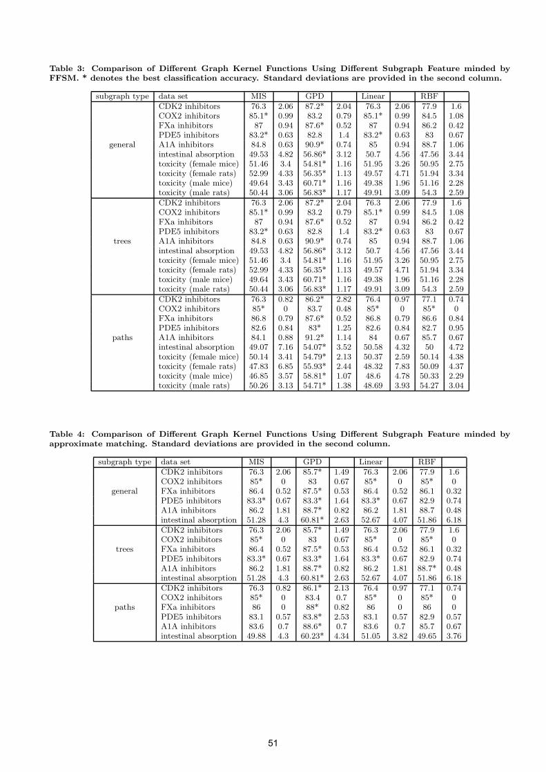
Table 3: Comparison of Different Graph Kernel Functions Using Different Subgraph Feature minded byFFSM. * denotes the best classification accuracy. Standard deviations are provided in the second column.

subgraph type data set MIS GPD Linear RBFCDK2 inhibitors 76.3 2.06 87.2* 2.04 76.3 2.06 77.9 1.6COX2 inhibitors 85.1* 0.99 83.2 0.79 85.1* 0.99 84.5 1.08FXa inhibitors 87 0.94 87.6* 0.52 87 0.94 86.2 0.42PDE5 inhibitors 83.2* 0.63 82.8 1.4 83.2* 0.63 83 0.67

general A1A inhibitors 84.8 0.63 90.9* 0.74 85 0.94 88.7 1.06intestinal absorption 49.53 4.82 56.86* 3.12 50.7 4.56 47.56 3.44toxicity (female mice) 51.46 3.4 54.81* 1.16 51.95 3.26 50.95 2.75toxicity (female rats) 52.99 4.33 56.35* 1.13 49.57 4.71 51.94 3.34toxicity (male mice) 49.64 3.43 60.71* 1.16 49.38 1.96 51.16 2.28toxicity (male rats) 50.44 3.06 56.83* 1.17 49.91 3.09 54.3 2.59CDK2 inhibitors 76.3 2.06 87.2* 2.04 76.3 2.06 77.9 1.6COX2 inhibitors 85.1* 0.99 83.2 0.79 85.1* 0.99 84.5 1.08FXa inhibitors 87 0.94 87.6* 0.52 87 0.94 86.2 0.42PDE5 inhibitors 83.2* 0.63 82.8 1.4 83.2* 0.63 83 0.67

trees A1A inhibitors 84.8 0.63 90.9* 0.74 85 0.94 88.7 1.06intestinal absorption 49.53 4.82 56.86* 3.12 50.7 4.56 47.56 3.44toxicity (female mice) 51.46 3.4 54.81* 1.16 51.95 3.26 50.95 2.75toxicity (female rats) 52.99 4.33 56.35* 1.13 49.57 4.71 51.94 3.34toxicity (male mice) 49.64 3.43 60.71* 1.16 49.38 1.96 51.16 2.28toxicity (male rats) 50.44 3.06 56.83* 1.17 49.91 3.09 54.3 2.59CDK2 inhibitors 76.3 0.82 86.2* 2.82 76.4 0.97 77.1 0.74COX2 inhibitors 85* 0 83.7 0.48 85* 0 85* 0FXa inhibitors 86.8 0.79 87.6* 0.52 86.8 0.79 86.6 0.84PDE5 inhibitors 82.6 0.84 83* 1.25 82.6 0.84 82.7 0.95

paths A1A inhibitors 84.1 0.88 91.2* 1.14 84 0.67 85.7 0.67intestinal absorption 49.07 7.16 54.07* 3.52 50.58 4.32 50 4.72toxicity (female mice) 50.14 3.41 54.79* 2.13 50.37 2.59 50.14 4.38toxicity (female rats) 47.83 6.85 55.93* 2.44 48.32 7.83 50.09 4.37toxicity (male mice) 46.85 3.57 58.81* 1.07 48.6 4.78 50.33 2.29toxicity (male rats) 50.26 3.13 54.71* 1.38 48.69 3.93 54.27 3.04

Table 4: Comparison of Different Graph Kernel Functions Using Different Subgraph Feature minded byapproximate matching. Standard deviations are provided in the second column.

subgraph type data set MIS GPD Linear RBFCDK2 inhibitors 76.3 2.06 85.7* 1.49 76.3 2.06 77.9 1.6COX2 inhibitors 85* 0 83 0.67 85* 0 85* 0

general FXa inhibitors 86.4 0.52 87.5* 0.53 86.4 0.52 86.1 0.32PDE5 inhibitors 83.3* 0.67 83.3* 1.64 83.3* 0.67 82.9 0.74A1A inhibitors 86.2 1.81 88.7* 0.82 86.2 1.81 88.7 0.48intestinal absorption 51.28 4.3 60.81* 2.63 52.67 4.07 51.86 6.18CDK2 inhibitors 76.3 2.06 85.7* 1.49 76.3 2.06 77.9 1.6COX2 inhibitors 85* 0 83 0.67 85* 0 85* 0

trees FXa inhibitors 86.4 0.52 87.5* 0.53 86.4 0.52 86.1 0.32PDE5 inhibitors 83.3* 0.67 83.3* 1.64 83.3* 0.67 82.9 0.74A1A inhibitors 86.2 1.81 88.7* 0.82 86.2 1.81 88.7* 0.48intestinal absorption 51.28 4.3 60.81* 2.63 52.67 4.07 51.86 6.18CDK2 inhibitors 76.3 0.82 86.1* 2.13 76.4 0.97 77.1 0.74COX2 inhibitors 85* 0 83.4 0.7 85* 0 85* 0

paths FXa inhibitors 86 0 88* 0.82 86 0 86 0PDE5 inhibitors 83.1 0.57 83.8* 2.53 83.1 0.57 82.9 0.57A1A inhibitors 83.6 0.7 88.6* 0.7 83.6 0.7 85.7 0.67intestinal absorption 49.88 4.3 60.23* 4.34 51.05 3.82 49.65 3.76

51

[4] Y. M. Bing Liu, Wynne Hsu. Integrating classification andassociation rule mining. In Proceedings of the FourthInternational Conference on Knowledge Discovery and DataMining, 1998.

[5] C. Chang and C. Lin. Libsvm: a library for support vectormachines, 2001. Software available athttp://www.csie.ntu.edu.tw/ cjlin/libsvm.

[6] M. Deshpande, M. Kuramochi, and G. Karypis. Frequentsub-structure-based approaches for classifying chemicalcompounds. IEEE Transactions on Knowledge and DataEngineering, 2005.

[7] Froohlich, J. Wegner, F. Sieker, and A. Zell. Kernel functionsfor attributed molecular graphs - a new similarity-basedapproach to adme prediction in classification. QSAR &Combinatorial Science, 2006.

[8] C. Helma, R. King, and S. Kramer. The predictive toxicologychallenge 2000-2001. Bioinformatics, 17(1):107–108, 2001.

[9] T. Horvath, T. Gartner, and S. Wrobel. Cyclic pattern kernelsfor predictive graph mining. SIGKDD, 2004.

[10] T. Horvath, J. Ramon, and S. Wrobel. Frequent subgraphmining in outerplanar graphs. In SIGKDD, 2006.

[11] J. Huan, W. Wang, and J. Prins. Efficient mining of frequentsubgraph in the presence of isomorphism. In Proceedings of the3rd IEEE International Conference on Data Mining (ICDM),pages 549–552, 2003.

[12] J. Huan, W. Wang, J. Prins, and J. Yang. SPIN: Miningmaximal frequent subgraphs from graph databases. pages581–586, 2004.

[13] J. Huan, W. Wang, A. Washington, J. Prins, R. Shah, andA. Tropsha. Accurate classification of protein structuralfamilies based on coherent subgraph analysis. In Proceedings ofthe Pacific Symposium on Biocomputing (PSB), pages411–422, 2004.

[14] Y. Huang, H. Li, H. Hu, X. Yan, M. S. Waterman, H. Huang,and X. J. Zhou. Systematic discovery of functional modules andcontext-specific functional annotation of human genome.Bioinformatics, pages ISMB/ECCB Supplement, 222–229,2007.

[15] A. Inokuchi, T. Washio, and H. Motoda. An apriori-basedalgorithm for mining frequent substructures from graph data.In PKDD’00, pages 13–23, 2000.

[16] W. W. J. Huan and J. Prins. Efficient mining of frequentsubgraphs in the presence of isomorphism. In Proc. of ICDM,2003.

[17] R. Jin, S. Mccalle, , and E. Almaas. Trend motif: A graphmining approach for analysis of dynamic complex networks.ICDM, 2007.

[18] R. Jorissen and M. Gilson. Virtual screening of moleculardatabases using a support vector machine. J. Chem. Inf.Model., 45(3):549–561, 2005.

[19] H. Kashima, K. Tsuda, and A. Inokuchi. Marginalized kernelsbetween labeled graphs. In Proc. of the Twentieth Int. Conf.on Machine Learning (ICML), 2003.

[20] Y. Ke, J. Cheng, , and W. Ng. Correlation search in graphdatabases. In SIGKDD, 2007.

[21] T. Kudo, E. Maeda, and Y. Matsumoto. An application ofboosting to graph classification. In NIPS, 2004.

[22] M. Kuramochi and G. Karypis. Frequent subgraph discovery. InProc. International Conference on Data Mining’01, pages313–320, 2001.

[23] S. Nijssen and J. Kok. A quickstart in frequent structuremining can make a difference. In Proceedings of the 10th ACMSIGKDD International Conference on Knowledge Discoveryand Data Mining, pages 647–652, 2004.

[24] J. R. Quinlan. C4.5 : Programs for Machine Learning.Morgan Kaufmann, 1993.

[25] L. Ravaliola, S. J. Swamidass, and H. Saigo. Graph kernels forchemical informatics. Neural Networks, 2005.

[26] D. Shasha, J. T. L. Wang, and R. Giugno. Algorithmics andapplications of tree and graph searching. In Proceeding of theACM Symposium on Principles of Database Systems(PODS), 2002.

[27] A. Smalter, J. Huan, and G. Lushington. Structure-basedpattern mining for chemical compound classification. InProceedings of the 6th Asia Pacific BioinformaticsConference, 2008.

[28] J. Sun, S. Papadimitriou, P. S. Yu, and C. Faloutsos.Parameter-free mining of large time-evolving graphs. InSIGKDD, 2007.

[29] N. Tolliday, P. A. Clemons, P. Ferraiolo, A. N. Koehler, T. A.

Lewis, X. Li, S. L. Schreiber, D. S. Gerhard, and S. Eliasof.Small molecules, big players: the national cancer institute’sinitiative for chemical genetics. Cancer Research, 66:8935–42,2006.

[30] H. Tong, Y. Koren, , and C. Faloutsos. Fast direction-awareproximity for graph mining. In SIGKDD, 2007.

[31] V. Vapnik. Statistical Learning Theory. John Wiley, 1998.

[32] N. Wale, I. Watson, , and G. Karypis. Comparison of descriptorspaces for chemical compound retrieval and classification.Knowledge and Information Systems, 2007.

[33] M. Wessel, P. Jurs, J. Tolan, and S. Muskal. Prediction ofhuman intestinal absorption of drug compounds from molecularstructure. J. Chem. Inf. Comput. Sci., 38(4):726–735, 1998.

[34] J. Weston, R. Kuang, C. Leslie, and W. S. Noble. Proteinranking by semi-supervised network propagation. BMCBioinformatics, 2006.

[35] D. Williams, J. Huan, and W. Wang. Graph database indexingusing structured graph decomposition. In in Proceedings of the23rd IEEE International Conference on Data Engineering(ICDE), 2007.

[36] X. Yan and J. Han. gspan: Graph-based substructure patternmining. In Proc. International Conference on DataMining’02, pages 721–724, 2002.

[37] X. Yan, P. S. Yu, and J. Han. Graph indexing based ondiscriminative frequent structure analysis. In ACMTransactions on Database Systems (TODS), 2005.

[38] M. J. Zaki and C. C. Aggarwal. Xrules: An effective structuralclassifier for xml data. Machine Learning Journal special issueon Statistical Relational Learning and Multi-Relational DataMining, 62, No. 1-2:137–170, 2006.

[39] Z. Zeng, J. Wang, L. Zhou, and G. Karypis. Coherent closedquasi-clique discovery from large dense graph databases. InSIGKDD, 2006.

[40] D. Zhou, J. Huang, and B. Schoolkopf. Learning from labeledand unlabeled data on a directed graph. Proceedings of the22nd International Conference on Machine Learning, 2005.

APPENDIX

A. CONNECTION OF PATTERN DIFFUSIONTO MARGINALIZED GRAPH KERNEL

Here we show the connection of pattern diffusion kernelfunction to the marginalized graph kernel [19], which usesa Markov model to randomly generate walks of a labeledgraph.

Given a graph G with nodes set V [G] = {v1, v2, . . . , vn},and a seed S ⊆ V [G], for each diffusion function ft, we con-struct a vector Ut = (ft(v1), ft(v2), . . . , ft(vn)). Accordingto the definition of ft, we have Ut+1 = Γ × Ut where thematrix Γ is defined as:

Γ(i, j) =

8

>

<

>

:

λd(vj)

if i 6= j and i ∈ N(j)

1 − λd(vi)

i = j

0 otherwise

In this representation, we compute the stationary distri-bution (fS = limt→∞ ft) by computing Γ∞ × U0.

We notice that the matrix Γ corresponds to a probabilitymatrix corresponding to a Markov Chain since

• all entries are non-negative

• column sum is 1 for each column

Therefore the vector Γ∞ ×U0 corresponds to the station-ary distribution of the local random walk as specified by Γ.In other words, rather than using random walk to retrieveinformation about the local topology of a graph, we use thestationary distribution to retrieve information about the lo-cal topology. Our experimental study shows that this in factis an efficient way for graph classification.

52

Reinforcing Mutual Information-based Strategy for FeatureSelection for Microarray Data

Jian TangDepartment of Computer Science

Memorial University of NewfoundlandSt. John’s, NL, Canada

jian@cs.mun.ca

Shuigeng Zhou Feng Li Kai JiangSchool of Computer Science, and

Shanghai Key Lab of Intelligent Information ProcessingFudan University, Shanghai 200433, China

{sgzhou,fengli2006,jiangkai}@fudan.edu.cn

ABSTRACTMutual information (MI) is a powerful concept for correlation-centric applications. Recently, it has been used for featureselection for microarray gene expression data. One of themerits of MI is, unlike many other heuristic methods, it isbased on a mature theoretic foundation. When applied tomicroarray data, however, it faces a number of challenges.Firstly, due to large numbers of features (i.e., genes) presentin microarrays, the true distributions for the expression val-ues of some genes may be masked by noises. Secondly, eval-uating inter-group mutual information requires estimatingmulti-variate distributions, which is difficult. To address thefirst problem, we use a scheme called Substantial relevanceboosting, which requires a non-noisy feature to show sub-stantially additional relevance with class labeling beyond thealready selected features. To address the second problem, weuse Increasing likelihood of feature interaction, which proba-bilistically compensates for feature interaction missing fromsimple aggregation-based simulation. We justify our strate-gies from both a theoretical perspective, and the experimen-tal results on real life data sets, which show the improvedeffectiveness of our method over the existing schemes.

Categories and Subject DescriptorsI.5.2 [Computing Methodologies]: Design Methodology—feature evaluation and selection

General TermsAlgorithms

KeywordsFeature selection, gene expression profiling, mutual informa-tion, classification, feature interaction

1. INTRODUCTIONDue to large numbers of features (i.e., genes) in microarray

gene expression data, some genes may seem to be relevant

Permission to make digital or hard copies of all or part of this work forpersonal or classroom use is granted without fee provided that copies arenot made or distributed for profit or commercial advantage and that copiesbear this notice and the full citation on the first page. To copy otherwise, torepublish, to post on servers or to redistribute to lists, requires prior specificpermission and/or a fee.BIOKDD ’08, August 24, 2008, Las Vegas, Nevada, USA.Copyright 2008 ACM 978-1-60558-302-0 ...$5.00.

to the class labeling, but in fact are biologically irrelevant.These ’noisy’ features can mislead the learning process, ren-dering traditional classification methods not being effective.Feature selection is a process to select truly relevant featureswith the class labeling. When the purpose of learning is toclassify unlabeled samples, the selected feature subset withsmall size is desirable. There are some good reasons for this.Small feature sizes imply less redundancies, which can im-prove inferences and classifications. Small feature sizes areless likely to over-fit, and therefore can increase generaliza-tion capability for classifiers. This is beneficial in clinicalsettings. In disease profiling, a small sized gene set that en-ables accurate classification may be potential diagnostic orprognostic markers. Because of this, minimizing the sizes offeature sets that enable accurate classifications has been thegoal of a large number of existing works on feature selectionfor gene expression data.

Mutual information (MI) is a powerful concept for correlation-centric applications. Recently, it has been used for featureselection for microarray gene expression data [4, 9, 10, 17].One of the merits of MI is that, unlike many other heuristicmethods, it has a mature theoretic foundation [8]. For adata set where many noisy features are present, however, itspower may diminish. In these data sets, the mutual infor-mation evaluated for noisy features may not reflect the truefacts. Another problem with MI in this context arises fromevaluation of inter-group mutual information. This normallyrequires estimating multivariate distributions, which in thegeneral case is difficult. Existing MI-based feature selectionmethods rank features according to their individual mutualinformation with class labeling, with the hope that noisyfeatures will be filtered out automatically. Redundancies areevaluated based on mutual information between a candidatefeature and the group of already-selected features. Estima-tion of multi-variate distribution is avoided by using simpleaggregation (e.g., averaging) over individual mutual infor-mation as an approximation for group mutual information.Since the simple aggregation is based on mutual informationindividually evaluated, it is incapable of simulating mutualinformation arising from feature interactions. (Refer to Sec-tion 2.2.4 for detail.)

MI-based feature selection belongs to the general categoryof individual-oriented scoring methods, which score genesindividually based on their ability to discriminate differentclasses, and measure redundancies using feature-feature cor-relation [4, 6, 9, 11, 16, 17, 19, 21]. These schemes allshared the two problems mentioned previously. A differ-ent category of group-oriented methods associates scores

53

with groups, rather than individual features [1, 5, 12, 15,20]. Higher scores are assigned to groups with higher rele-vance with class labeling and smaller redundancies amongthe group members. The actual scoring mechanisms usedare quite diverse. Focus [1] systematically searches for afeature set that has consistent discriminative power withthe full feature set. Its search method is essentially exhaus-tive, and costly in high dimensional space. In [15], the au-thors introduce Markov-blanket to detect effectively redun-dant features at the conceptual level. It is however difficultto implement in practice since it requires estimating multi-variate densities. The same problem is shared by the workin [5]. Some work relaxes this requirement. The correlation-based feature selection [12] uses a metric that requires onlyestimating bi-variant densities, at the price of reduced ca-pability of describing relevance and redundancy. The fast-correlation-based feature selection proposed in [23] approx-imates Markov blanket. It is a powerful model. However, itrequires estimating tri-variate densities. The scheme in [24]uses as the group criteria the leave-one-out cross validationerrors based on least-square SVM (i.e., LS-SVM) classifiers.The error is actually generated by solving a linear systemof equations for the training set, and therefore avoids re-peated LOOCV applications. However, solving the linearsystem of equations is still sometime time consuming. Also,it is unclear how this technique can be applied to data setswith more than two classes. The work in [22] uses princi-ple component technique to select features. However, thereis no discussion of how effective this approach is in dealingwith redundancies. Recently, some work studies margin-based schemes, which score features based on the maximummargins they can exert between different classes [18]. Theyare essentially individual-oriented methods mentioned previ-ously, but can be conveniently extended to kernel spaces [3,7, 20]. However, these schemes normally are not concernedwith redundancies.

In this paper, we propose a group-oriented, MI-based fea-ture selection scheme. Our scheme uses explicit mechanismsto relieve the two problems mentioned previously. To ad-dress the first problem, we use a mechanism called Substan-tial relevance boosting, which requires a non-noisy featureto show substantially additional relevance with class label-ing beyond the already selected features. To address thesecond problem, we use Increasing likelihood of feature in-teraction, which probabilistically compensates for feature in-teraction missing from simple aggregations. In our scheme,it is only required to estimate bi-variant densities. We jus-tify our strategies from both a theoretical perspective, andthe experimental results on real life data sets, which showthe improved effectiveness of our method over the existingschemes.

The rest of paper is organized as follows. In Section 2, weprovide basic concepts that will be used in the subsequentsections, and then introduce our method. In section 3, wepresent the experimental results. We conclude the paper bysummarizing the main results.

2. SELECTING RELEVANT FEATURES

2.1 A metric for relevancy and redundancyOur definitions relating to mutual information are based

on the concepts from information theory [8]. Let X and Y

be two variables (features) and C be a set of class labels. The

entropy of X is defined as: H(X) = −∑

Dom(X)p(x)log(p(x)).

The conditional entropy of X given Y isH(X|Y ) = −

∑Dom(X)

∑Dom(Y )

p(x, y)log(p(x|y)). Theentropy of a variable measures the amount of uncertaintyof the variable. (If X and/or Y are sets of variables, theabove definitions still hold.) The mutual information of Xand Y is: I(X; Y ) = H(X)−H(X|Y ). Note that I(X; Y ) =I(Y ; X) = H(X) + H(Y ) − H(X,Y ). The mutual infor-mation of X and Y given Z is: I(Y ; X|Z) = H(Y |Z) −H(Y |Z, X). Also note that we have I(X; Y |Z) = I(Y ; X|Z)= H(X|Z)+H(Y |Z)−H(X,Y |Z). Let C be the target class.We say I(X; C) is the relevance of X to C. Let X and Y

be features, we also use I(X;Y ) to measure the amount ofredundancy of X and Y . It is easy to verify that if X and Y

are independent, then their redundancy is 0. On the otherhand, if they are fully dependent of each other, i.e., they are(essentially) duplicates, then their redundancy is H(X) orH(Y ).

2.2 Feature selections based on mutual infor-mation

2.2.1 General criteriaLet C be the target class, and F be the entire set of fea-

tures. We can view C and each feature in F as a randomvariable, and F as an n-variate. In theory, our goal is tosearch for a subset D = arg maxS⊆F I(S;C). That is, D isthe subset most relevant to the target class. In the generalcase, the desired subset is not unique. We would also like itto be of a smallest size, implying that it contains least redun-dancy. In practice, however, that expression is difficult toevaluate since the size of the search space is 2|F |. To reducethe search space, we may use a local optimization criterion.Let S be the current feature set, which is initialized to φ.We search for the next feature g to be included into S if:

g = arg maxe∈F−S

{I(e;C|S)} (1)

I(g;C|S) > 0 (2)

The conditional mutual information of e and C given S

is the information that e has about C given S. This isthe information that is not subsumed by the informationgiven in S about C. Therefore, both relevance and redun-dancy have been taken care of. We select g if it results inthis information being positive and maximized. With theabove criterion, we can use a forward hill climbing methodto search for features one at a time in an incremental fash-ion, and therefore drastically cut the search space, at theprice of returning local optimum only. However, if we usethat criterion as is for microarray data, a problem may arise,as described in the next section.

2.2.2 Substantial relevance boostingFrom the information theory, I(e;C|S) = 0 if and only if

e is conditionally independent of C given S. If e is indeedconditionally independent of C given S, and the distributiondemonstrated by the training set is a good approximation ofthe true distribution for the variables, then we can expectthat e will be close to being conditionally independent of C

given S reflected from the training set. However, as men-tioned previously, due to the fact that genes in typical mi-croarray datasets greatly outnumber sample examples, the

54

distributions described by the training set may not accu-rately reveal the true distributions of the variables. Thus abiologically irrelevant or redundant gene may turn out notto be very close to being conditionally independent of theclass labeling, resulting in I(s;C|S) not being close to zerowhen estimated based on the values in the training set. Wenow make the following assumption:

If e is biologically irrelevant to C given S, thenI(e;C|S)/H(C|S) based on the microarray datasetwill not be substantially larger than 0.

In other words, we allow a true conditional irrelevant geneto deviate in the distribution reflected in the training setfrom its true distribution for certain amount, which shouldnot be too large. We believe this assumption is reason-able for most of the microarray datasets which have a priorigone through pre-processing stages, in which many artifactsand variations have been eliminated. The amount of de-viation is measured by the ratio I(e; C|S)/H(C|S), whichis proportional to I(e;C|S), but inversely proportional toH(C|S). The rationale for the former is easy to see: shoulde’s true distribution be preserved in the training set, thenwe would have I(e;C|S) = 0. Thus, a larger value forI(e;C|S) signifies a larger departure from e’s true distri-bution. For the latter, recall that H(C|S) is the amountof uncertainty that remains in C when S is present, andI(e;C|S) = H(C|S) − H(C|S, e) is the amount of uncer-tainty further deducted from C when e is present. Such afurther deduction requires e to have the information that S

does not have. A low value of H(C|S) implies S containsa lot of information about C, and therefore requires e todeviate more to possess additional information to what S

already has.Based on the above assumption, we replace condition (2)

by a stronger condition:

I(g;C|S)/H(C|S) > α (3)

where α is a threshold set by users. Note that it is easy toverify I(g;C|S) = I(S, g; C) − I(S; C). Let S be a set offeatures already selected. According to our terminologies,we can view I(g;C|S) as a measure of the relevance with C

by in addition to I(S; C) due to g’s presence. Thus we callcondition (3) substantial relevance boosting, where α imple-ments substantiality. A critical issue, of course, is how to seta proper value for α. Too large a value would filter out notonly irrelevant features, but also some relevant ones, whiletoo small a value would weaken the filtering power. We havedone extensive testing, and found that the best value for α

is between 0.05 and 0.15, and is almost invariant for all thedata sets in our experiment. (Refer to Section 3.)

2.2.3 Computing relevanceA practical issue is how to estimate a conditional mutual

information. Our goal is to develop approximations that pre-serve its basic characteristics, and at the same time possessreasonable applicability. We first introduce an assertion.

Assertion 1. Let S ⊂ F and e ∈ F − S. Then

I(e;C|S) = I(S,C; e)− I(S; e) (4)

Proof. The chain rule of entropy states that, for anyvariable A, and set of variables R, it is true that H(R,A) =H(R) + H(A|R). Based on this, we have

I(e;C|S)= H(C|S)−H(C|S, e)= H(C,S)−H(S)− (H(C,S, e)−H(S, e))= H(S,C)+H(e)−H(S, e,C)− (H(S)+H(e)−H(S, e))= I(S,C; e)− I(S; e)

Thus, given feature set S and labeling C, maximizingI(e;C|S) is equivalent to maximizing the difference on theright side of (4). Since we are unable to actually maximizethat difference, we will use approximations for the two termson the right hand side of (4). In the following, for any X

and Y , we use I(X; Y ) for the approximation of I(X; Y )calculated using a different formula from its definition.

I(S, C; e) =|S|

|S|+ 1I(S; e) +

1

|S|+ 1I(C; e) (5)

I(S; e) =1

|S|

∑

x∈S

I(x; e) (6)

Substituting the right side of formulas (5) into (4), and

then replace I(S; e) by I(S; e), we have the following

I(e, S; C)− I(S; C) =1

|S|+ 1I(e; C)−

1

|S|+ 1I(e; S) (7)

Formula (7) will be used to simulate formula (4). Observe

that larger value for I(e; S), or smaller value for I(e;C), re-sults in smaller amount to be added to the (approximated)

relevance of S to C. If we use I(e, S; C) − I(S; C) to simu-late I(e;C|S), we must maximize the former. This is equiv-

alent to maximizing I(e;C) − I(e; S). Note that the lastmaximization operation requires estimating bi-variant den-sities only. Now the question is: how do we justify maxi-

mizing I(e, S; C) − I(S; C) in terms of the effectiveness offeature selection, not just in terms of the effectiveness ofmulti-variate density estimations. After all, our ultimatepurpose is to maximize I(e;C|S). From formula (5) and(6), it is not immediately clear how the maximum value for

I(e, S; C)− I(S; C) can boost the value of I(e;C|S).

Assertion 2. The following inequality is true:

I(e;C|S) ≤ I(e;C)− I(e; S) + H(S|C) (8)

Proof. First, by chain rule for mutual information, I(S,C; e) =I(C; e) + I(S; e|C), we have the following:

I(S,C; e)− I(S; e)= I(C; e)− I(S; e) + I(S; e|C)= I(C; e)− I(S; e) + H(S|C)−H(S|C, e)≤ I(C; e)− I(S; e) + H(S|C)= I(e;C)− I(e;S) + H(S|C)On the other hand, by the information theory, for any

x ∈ S, I(e;S) ≥ I(e; x). Thus I(e;S) ≥ 1

|S|

∑x∈S

I(e;x) =

I(e;S) . This implies I(S,C; e)−I(S; e) ≤ I(e; C)−I(e;S)+H(S|C). Inequality (8) then follows from Assertion 1

Assertion 2 establishes an upper bound for I(e;C|S). WhenS and C are given, the term H(S|C) is a constant. Thus,

maximizing I(e;C) − I(e; S) actually maximizes this up-per bound, which approximates the criterion of maximizingI(e;C|S). The expected effect of this approximation is thehigh likelihood that a large value for I(e;C|S) will be ob-tained. In the following section, we will use a strategy thatadditionally promotes such a likelihood.

55

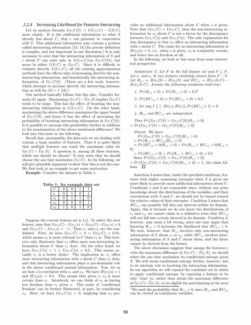
2.2.4 Increasing Likelihood for Features InteractingLet us analyze formula I(e;C|S) = I(S, e; C) − I(S; C)

more closely. It is the additional information to what S

already has about C, that e can generate in cooperationwith S. This additional information may contain a portioncalled interacting information [13, 14].(Its precise definitionis complex, and not important in our discussion.) It is onlynecessary to note that the interacting information of S ande about C can exist only in I(S, e; C)(or I(e; C|S)), butnever in either I(S; C) or I(e;C). Since it is difficult toevaluate directly I(S, e;C), all the existing approximationmethods have the effects only of increasing directly the non-interacting information, and heuristically the interacting in-formation, of I(e;C|S). (There are a few work, however,which attempt to increase directly the interacting informa-tion as well for |S| = 1 [16].)

Our method basically follows this line also. Consider for-

mula (8) again. Maximizing I(e;C)− I(e;S) implies I(e;C)tends to be large. This has the effect of boosting the non-interacting information in I(S, e; C). On the other hand,maximizing the above difference maximizes the upper boundof I(e;C|S), and hence it has the effect of increasing theprobability of boosting interacting information in I(e;C|S).Is it possible to increase this probability further in additionto the maximization of the above mentioned difference? Welook into this issue in the following.

Recall that, presumably, the data sets we are dealing withcontain a large number of features. Thus it is quite likelythat multiple features can reach the maximum value for

I(e;C) − I(e; S). A question is, among all these features,which one should we choose? It may seem that we shouldchoose the one that maximizes I(e;C). In the following, wewill give plausible argument to show that this is not the case.We first look at an example to get some motivation.

Exmple: Consider the dataset in Table 1.

Table 1: An example data setC 0 0 1 1s 0 1 0 1e1 0 1 1 0e2 0 0 0 1e3 1 0 1 0

Suppose the current feature set is {s}. To select the nextfeature, note that I(e1; C)−I(e1; s) = I(e2; C)−I(e2; s) = 0and I(e3; C) − I(e3; s) = −1. Thus e1 and e2 are the can-didates. First, we have I(e1; C) = 0 < I(e2; C) = 0.31,which means e2 is more relevant to C than e1 is. This how-ever only illustrates that e2 offers more non-interacting in-formation about C than e1 does. On the other hand, wehave I(e1; C|s) = 1 > I(e2; C|s) = 0.5. This means ac-tually e1 is a better choice. The implication is, e1 offersmore interacting information with s about C than e2 does,and this interacting information plays a pre-dominant rolein the above conditional mutual information. Now, let ussee how s is correlated with e1 and e2. We have H(e1|s) = 1and H(e2|s) = 0.5. This means that given s, e2 is morecertain than e1. Intuitively, we can think of e2 as havingless freedom than e1 given s. This point of ’conditionalfreedom’ can be further illustrated, in part, by consideringe3. Here, we have I(e3; C|s) = 0, implying that e3 pro-

vides no additional information about C when s is given.Note that I(e1; C) = I(e3; C), thus the non-interacting in-formation by e3 about C is not a factor for the discrepancybetween I(e1; C|s) and I(e3; C|s). The only explanation forthis discrepancy is that e3 offers no interacting informationwith s about C. The cause for no interacting information isH(e3|s) = 0, i.e., when s is given, e3 is completely certain,and hence has no freedom at all.

In the following, we look at this issue from some theoret-ical perspective.

Assertion 3. Let F be the full feature set and S ⊆ F .Let ei and ej be two features randomly chosen from F − S.Let Hi,j = H(ei|S) − H(ej|S) and HCi,j = H(ei|S, C) −H(ej |S, C). Assume the following conditions hold true:

1. Pr(Hi,j > 0) = Pr(Hi,j < 0) = 0.51

2. Pr(HCi,j > 0) = Pr(HCi,j < 0) = 0.5

3. for any I ⊆ [−H(ej), H(ei)], P r(HCi,j ∈ I) > 0

4. Hi,j and HCi,j are independent.

Then Pr(I(ei; C|S) > I(ej; C|S)|Hi,j > 0

)

> Pr(I(ej; C|S) > I(ei; C|S)|Hi,j > 0

)

Proof. We have:Pr(I(ei; C|S) > I(ej ; C|S)|Hi,j > 0)

= Pr(Hi,j > HCi,j |Hi,j > 0)= Pr(HCi,j < 0|Hi,j > 0) + Pr(Hi,j > HCi,j > 0|Hi,j >

0)= Pr(HCi,j < 0) + Pr(Hi,j > HCi,j > 0) > 0.5Since Pr

(I(ei; C|S) > I(ej ; C|S)|Hi,j > 0

)

+ Pr(I(ej ; C|S) > I(ei; C|S)|Hi,j > 0

)= 1, the claim fol-

lows.

Assertion 3 states that, under the specified conditions, fea-tures with higher remaining entropies when S is given aremore likely to provide more additional information about C.Conditions 1 and 2 are reasonable since, without any priorknowledge about the distributions of the variables, and theircorrelations with S and C, we should not be biased towardthe relative values of their entropies. Condition 3 states thatHCi,j can possibly fall into any interval within its domain.Again, this is because we do not know the distributions ofei and ej , we cannot claim in a definitive term that HCi,j

will not fall into certain interval in its domain. Condition 4,however, may seem a bit strong, since one may argue thatknowing Hi,j > 0 increases the likelihood that HCi,j > 0.We note, however, that Hi,j involves only non-interactinginformation of S about ei or ej , while HCi,j involves inter-acting information of S and C about them, and the lattercannot be derived from the former.

The above discussion suggests that among the features e

with the maximum difference of I(e;C)− I(e; S), we shouldselect the one that maximizes its conditional entropy givenS. We will stress conditional entropy further, however, dueto its intrinsic role in boosting the interacting information.In our algorithm we will expand the candidate set in whichto apply conditional entropy, by requiring a feature to beonly ’close’ to, rather than attain the maximum difference

of I(e;C)−I(e;S), to be eligible for participating in the next

1We omit the probability that Hi,j = 0, since Hi,j and HCi,j

can be viewed as continuous variables.

56

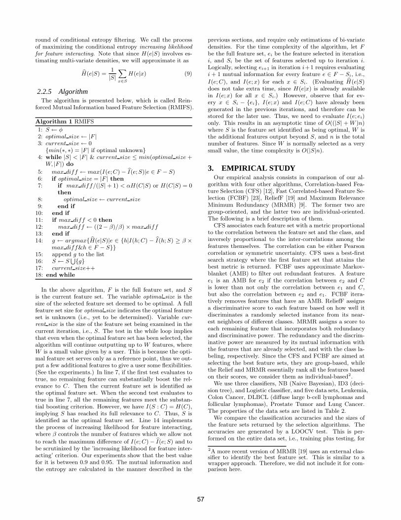
round of conditional entropy filtering. We call the processof maximizing the conditional entropy increasing likelihoodfor feature interacting. Note that since H(e|S) involves es-timating multi-variate densities, we will approximate it as

H(e|S) =1

|S|

∑

x∈S

H(e|x) (9)

2.2.5 AlgorithmThe algorithm is presented below, which is called Rein-

forced Mutual Information based Feature Selection (RMIFS).

Algorithm 1 RMIFS

1: S ← φ

2: optimal size← |F |3: current size← 0{min(∗, ∗) = |F | if optimal unknown}

4: while |S| < |F | & current size ≤ min(optimal size +W, |F |) do

5: max diff ← max(I(e;C) − I(e;S)|e ∈ F − S)6: if optimal size = |F | then7: if max diff/(|S| + 1) < αH(C|S) or H(C|S) = 0

then8: optimal size← current size

9: end if10: end if11: if max diff < 0 then12: max diff ← ((2− β)/β) ×max diff

13: end if14: g ← argmax{H(e|S)|e ∈ {h|I(h; C) − I(h; S) ≥ β ×

max diff&h ∈ F − S}}15: append g to the list16: S ← S

⋃{g}

17: current size++18: end while

In the above algorithm, F is the full feature set, and S

is the current feature set. The variable optimal size is thesize of the selected feature set deemed to be optimal. A fullfeature set size for optimal size indicates the optimal featureset is unknown (i.e., yet to be determined). Variable cur-rent size is the size of the feature set being examined in thecurrent iteration, i.e., S. The test in the while loop impliesthat even when the optimal feature set has been selected, thealgorithm will continue outputting up to W features, whereW is a small value given by a user. This is because the opti-mal feature set serves only as a reference point, thus we out-put a few additional features to give a user some flexibilities.(See the experiments.) In line 7, if the first test evaluates totrue, no remaining feature can substantially boost the rel-evance to C. Then the current feature set is identified asthe optimal feature set. When the second test evaluates totrue in line 7, all the remaining features meet the substan-tial boosting criterion. However, we have I(S : C) = H(C),implying S has reached its full relevance to C. Thus, S isidentified as the optimal feature set. Line 14 implementsthe process of increasing likelihood for feature interacting,where β controls the number of features which we allow not

to reach the maximum difference of I(e;C)− I(e; S) and tobe scrutinized by the ’increasing likelihood for feature inter-acting’ criterion. Our experiments show that the best valuefor it is between 0.9 and 0.95. The mutual information andthe entropy are calculated in the manner described in the

previous sections, and require only estimations of bi-variatedensities. For the time complexity of the algorithm, let F

be the full feature set, ei be the feature selected in iterationi, and Si be the set of features selected up to iteration i.Logically, selecting ei+1 in iteration i+1 requires evaluatingi + 1 mutual information for every feature e ∈ F − Si, i.e.,

I(e;C), and I(e;x) for each x ∈ Si. (Evaluating H(e|S)does not take extra time, since H(e|x) is already availablein I(e;x) for all x ∈ Si.) However, observe that for ev-ery x ∈ Si − {ei}, I(e;x) and I(e;C) have already beengenerated in the previous iterations, and therefore can bestored for the later use. Thus, we need to evaluate I(e; ei)only. This results in an asymptotic time of O((|S| + W )n)where S is the feature set identified as being optimal, W isthe additional features output beyond S, and n is the totalnumber of features. Since W is normally selected as a verysmall value, the time complexity is O(|S|n).

3. EMPIRICAL STUDYOur empirical analysis consists in comparison of our al-

gorithm with four other algorithms, Correlation-based Fea-ture Selection (CFS) [12], Fast Correlated-based Feature Se-lection (FCBF) [23], ReliefF [19] and Maximum RelevanceMinimum Redundancy (MRMR) [9]. The former two aregroup-oriented, and the latter two are individual-oriented.The following is a brief description of them.

CFS associates each feature set with a metric proportionalto the correlation between the feature set and the class, andinversely proportional to the inter-correlations among thefeatures themselves. The correlation can be either Pearsoncorrelation or symmetric uncertainty. CFS uses a best-firstsearch strategy where the first feature set that attains thebest metric is returned. FCBF uses approximate Markov-blanket (AMB) to filter out redundant features. A featuree1 is an AMB for e2 if the correlation between e2 and C

is lower than not only the correlation between e1 and C,but also the correlation between e2 and e1. FCBF itera-tively removes features that have an AMB. ReliefF assignsa discriminative score to each feature based on how well itdiscriminates a randomly selected instance from its near-est neighbors of different classes. MRMR assigns a score toeach remaining feature that incorporates both redundancyand discriminative power. The redundancy and the discrim-inative power are measured by its mutual information withthe features that are already selected, and with the class la-beling, respectively. Since the CFS and FCBF are aimed atselecting the best feature sets, they are group-based, whilethe Relief and MRMR essentially rank all the features basedon their scores, we consider them as individual-based2.

We use three classifiers, NB (Naive Bayesian), ID3 (deci-sion tree), and Logistic classifier, and five data sets, Leukemia,Colon Cancer, DLBCL (diffuse large b-cell lymphomas andfollicular lymphomas), Prostate Tumor and Lung Cancer.The properties of the data sets are listed in Table 2.

We compare the classification accuracies and the sizes ofthe feature sets returned by the selection algorithms. Theaccuracies are generated by a LOOCV test. This is per-formed on the entire data set, i.e., training plus testing, for

2A more recent version of MRMR [19] uses an external clas-sifier to identify the best feature set. This is similar to awrapper approach. Therefore, we did not include it for com-parison here.

57

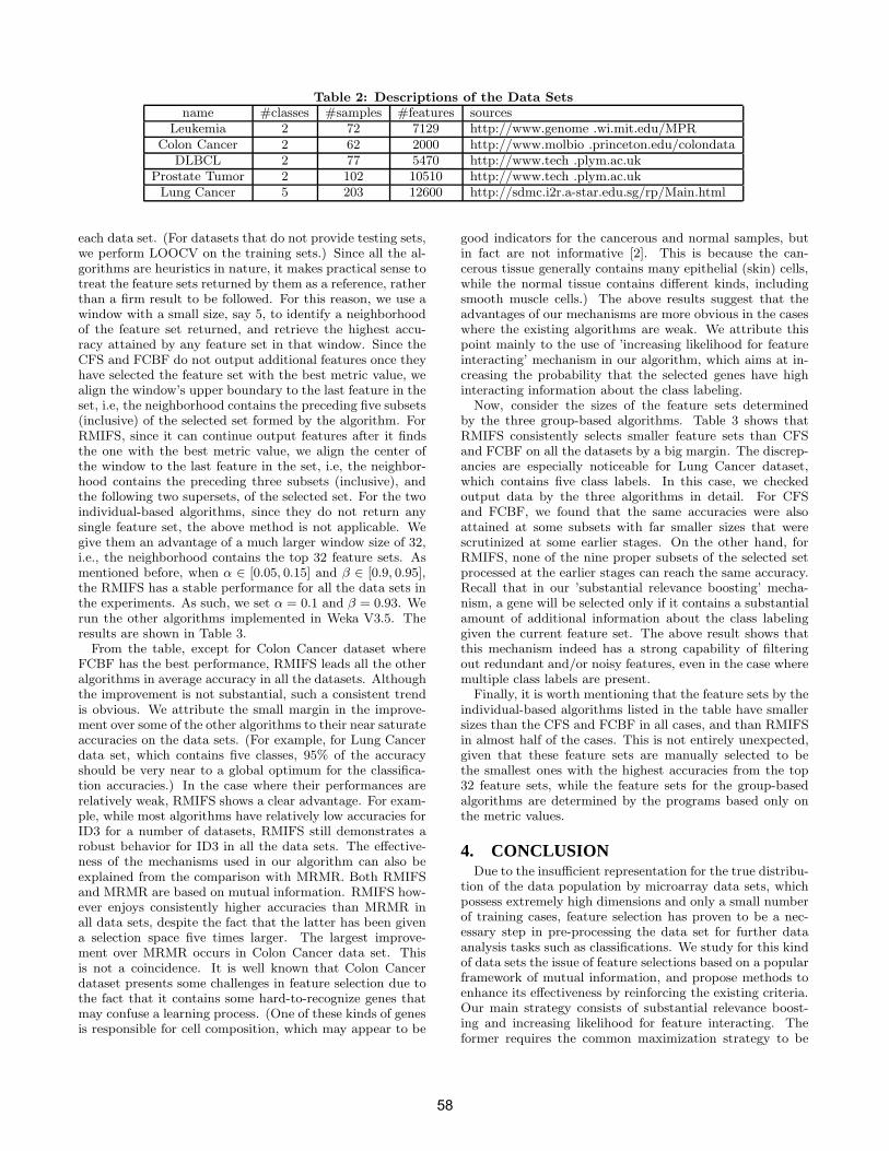
Table 2: Descriptions of the Data Setsname #classes #samples #features sources

Leukemia 2 72 7129 http://www.genome .wi.mit.edu/MPRColon Cancer 2 62 2000 http://www.molbio .princeton.edu/colondata

DLBCL 2 77 5470 http://www.tech .plym.ac.ukProstate Tumor 2 102 10510 http://www.tech .plym.ac.uk

Lung Cancer 5 203 12600 http://sdmc.i2r.a-star.edu.sg/rp/Main.html

each data set. (For datasets that do not provide testing sets,we perform LOOCV on the training sets.) Since all the al-gorithms are heuristics in nature, it makes practical sense totreat the feature sets returned by them as a reference, ratherthan a firm result to be followed. For this reason, we use awindow with a small size, say 5, to identify a neighborhoodof the feature set returned, and retrieve the highest accu-racy attained by any feature set in that window. Since theCFS and FCBF do not output additional features once theyhave selected the feature set with the best metric value, wealign the window’s upper boundary to the last feature in theset, i.e, the neighborhood contains the preceding five subsets(inclusive) of the selected set formed by the algorithm. ForRMIFS, since it can continue output features after it findsthe one with the best metric value, we align the center ofthe window to the last feature in the set, i.e, the neighbor-hood contains the preceding three subsets (inclusive), andthe following two supersets, of the selected set. For the twoindividual-based algorithms, since they do not return anysingle feature set, the above method is not applicable. Wegive them an advantage of a much larger window size of 32,i.e., the neighborhood contains the top 32 feature sets. Asmentioned before, when α ∈ [0.05, 0.15] and β ∈ [0.9, 0.95],the RMIFS has a stable performance for all the data sets inthe experiments. As such, we set α = 0.1 and β = 0.93. Werun the other algorithms implemented in Weka V3.5. Theresults are shown in Table 3.

From the table, except for Colon Cancer dataset whereFCBF has the best performance, RMIFS leads all the otheralgorithms in average accuracy in all the datasets. Althoughthe improvement is not substantial, such a consistent trendis obvious. We attribute the small margin in the improve-ment over some of the other algorithms to their near saturateaccuracies on the data sets. (For example, for Lung Cancerdata set, which contains five classes, 95% of the accuracyshould be very near to a global optimum for the classifica-tion accuracies.) In the case where their performances arerelatively weak, RMIFS shows a clear advantage. For exam-ple, while most algorithms have relatively low accuracies forID3 for a number of datasets, RMIFS still demonstrates arobust behavior for ID3 in all the data sets. The effective-ness of the mechanisms used in our algorithm can also beexplained from the comparison with MRMR. Both RMIFSand MRMR are based on mutual information. RMIFS how-ever enjoys consistently higher accuracies than MRMR inall data sets, despite the fact that the latter has been givena selection space five times larger. The largest improve-ment over MRMR occurs in Colon Cancer data set. Thisis not a coincidence. It is well known that Colon Cancerdataset presents some challenges in feature selection due tothe fact that it contains some hard-to-recognize genes thatmay confuse a learning process. (One of these kinds of genesis responsible for cell composition, which may appear to be

good indicators for the cancerous and normal samples, butin fact are not informative [2]. This is because the can-cerous tissue generally contains many epithelial (skin) cells,while the normal tissue contains different kinds, includingsmooth muscle cells.) The above results suggest that theadvantages of our mechanisms are more obvious in the caseswhere the existing algorithms are weak. We attribute thispoint mainly to the use of ’increasing likelihood for featureinteracting’ mechanism in our algorithm, which aims at in-creasing the probability that the selected genes have highinteracting information about the class labeling.

Now, consider the sizes of the feature sets determinedby the three group-based algorithms. Table 3 shows thatRMIFS consistently selects smaller feature sets than CFSand FCBF on all the datasets by a big margin. The discrep-ancies are especially noticeable for Lung Cancer dataset,which contains five class labels. In this case, we checkedoutput data by the three algorithms in detail. For CFSand FCBF, we found that the same accuracies were alsoattained at some subsets with far smaller sizes that werescrutinized at some earlier stages. On the other hand, forRMIFS, none of the nine proper subsets of the selected setprocessed at the earlier stages can reach the same accuracy.Recall that in our ’substantial relevance boosting’ mecha-nism, a gene will be selected only if it contains a substantialamount of additional information about the class labelinggiven the current feature set. The above result shows thatthis mechanism indeed has a strong capability of filteringout redundant and/or noisy features, even in the case wheremultiple class labels are present.

Finally, it is worth mentioning that the feature sets by theindividual-based algorithms listed in the table have smallersizes than the CFS and FCBF in all cases, and than RMIFSin almost half of the cases. This is not entirely unexpected,given that these feature sets are manually selected to bethe smallest ones with the highest accuracies from the top32 feature sets, while the feature sets for the group-basedalgorithms are determined by the programs based only onthe metric values.

4. CONCLUSIONDue to the insufficient representation for the true distribu-

tion of the data population by microarray data sets, whichpossess extremely high dimensions and only a small numberof training cases, feature selection has proven to be a nec-essary step in pre-processing the data set for further dataanalysis tasks such as classifications. We study for this kindof data sets the issue of feature selections based on a popularframework of mutual information, and propose methods toenhance its effectiveness by reinforcing the existing criteria.Our main strategy consists of substantial relevance boost-ing and increasing likelihood for feature interacting. Theformer requires the common maximization strategy to be

58

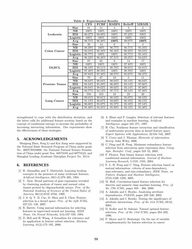
Table 3: Experimental ResultsCFS FCBF RMIFS ReliefF MRMR

Size 81 51 4 3 2NB 100% 100% 100% 100% 100%

Leukemia ID3 90.27% 88.89% 100% 97.22% 100%Logistic 100% 100% 100% 100% 100%

Avg 96.75% 96.30% 100% 99.07% 100%Size 26 14 6 7 4NB 98.39% 100% 96.77% 88.71% 95.16%

Colon Cancer ID3 93.55% 95.16% 95.16% 90.32% 93.55%Logistic 96.77% 100% 100% 88.71% 95.16%

Avg 96.23% 98.38% 97.31% 89.25% 94.62%Size 87 65 6 14 17NB 100% 100% 100% 97.40% 100%

DLBCL ID3 96.10% 93.51% 98.70% 90.91% 94.81%Logistic 97.40% 98.70% 100% 98.70% 100%

Avg 97.83% 97.40% 99.57% 95.67% 98.27%Size 79 67 10 5 11NB 98.04% 98.04% 98.04% 93.14% 98.04%

Prostate Tumor ID3 88.24% 85.29% 96.08% 93.14% 97.06%Logistic 98.04% 99.02% 99.02% 93.14% 97.06%

Avg 94.77% 94.12% 97.71% 93.14% 97.39%Size 550 453 10 23 26NB 99.01% 99.01% 98.52% 95.07% 98.52%

Lung Cancer ID3 91.13% 88.67% 93.60% 88.18% 90.15%Logistic 96.06% 95.07% 95.57% 93.10% 97.54%

Avg 95.40% 94.25% 95.89% 92.12% 95.40%

strengthened to cope with the distribution deviation, andthe latter calls for additional feature scrutiny based on theconcept of conditional entropy to increase the probability ofincreasing interacting information. Our experiments showthe effectiveness of these strategies.

5. ACKNOWLEDGEMENTSShuigeng Zhou, Feng Li and Kai Jiang were supported by

the National Basic Research Program of China under grantNo. 2007CB310806, the National Natural Science Founda-tion of China under grant Nos. 60573183 and 60773123, andShanghai Leading Academic Discipline Project No. B114.

6. REFERENCES

[1] H. Almuallim and T. Dietterich. Learning booleanconcepts in the presence of many irrelevant features.Artificial Intelligence, 69(1-2):279–305, 1994.

[2] U. Alon. Broad patterns of gene expression revealedby clustering analysis of tumor and normal colontissues probed by oligonucleotide arrays. Proc. of theNational Academy of Sciences of the United States ofAmerica, 96(12):6745–6750, 1999.

[3] J. S. Q. Y. B. Cao, D. Shen and Z. Chen. Featureselection in a kernel space. Proc. of the 24th ICML,227:121–128, 2007.

[4] R. Battiti. Using mutual information for selectingfeatures in supervised neural net learning. IEEETrans. On Neural Networks, 5(4):537–550, 1994.

[5] D. Bell and H. Wang. A formalism for relevance andits application in feature subset selection. MachineLearning, 41(2):175–195, 2000.

[6] A. Blum and P. Langley. Selection of relevant featuresand examples in machine learning. ArtificialIntelligence, pages 245–271, 1997.

[7] H. Cho. Nonlinear feature extraction and classificationof multivariate process data in kernel feature space.Expert Systems with Applications, 32:534–542, 2007.

[8] T. Cover and J. Thomas. Elements of informationtheory. John Wiley, 2006.

[9] C. Ding and H. Peng. Minimum redundancy featureselection from microarray gene expression data. Comp.Syts. Bioinfor. Conf., pages 523–52, 2003.

[10] F. Fleuret. Fast binary feature selection withconditional mutual information. Journal of MachineLearning Research, 5:1531–1555, 2004.

[11] F. L. H. Peng and C. Ding. Feature selection based onmutual information: criteria of max-dependency,max-relevance, and min-redundancy. IEEE Trans. onPattern Analysis and Machine Intelligence,27(8):1226–1238, 2005.

[12] M. Hall. Correlation-based feature selection fordiscrete and numeric class machine learning. Proc. ofthe 17th ICML, pages 359 – 366, 2000.

[13] A. Jakulin and I. Bratko. Analyzing attributedependencies. PAKDD, pages 229–240, 2003.

[14] A. Jakulin and I. Bratko. Testing the significance ofattribute interactions. Proc. of the 21st ICML, 69:52,2004.

[15] D. Koller and M. Sahami. Toward optimal featureselection. Proc. of the 13rd ICML, pages 284–292,1996.

[16] P. Meyer and G. Bontempi. On the use of variablecomplementarity for feature selection in cancer

59

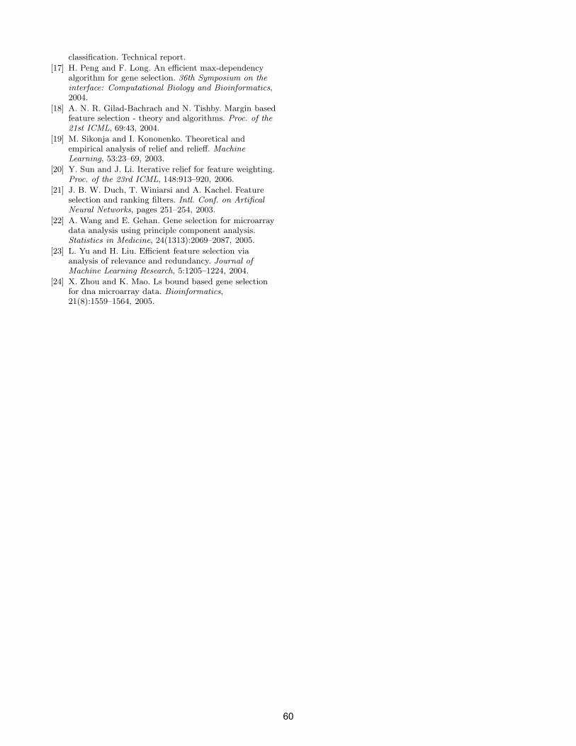
classification. Technical report.

[17] H. Peng and F. Long. An efficient max-dependencyalgorithm for gene selection. 36th Symposium on theinterface: Computational Biology and Bioinformatics,2004.

[18] A. N. R. Gilad-Bachrach and N. Tishby. Margin basedfeature selection - theory and algorithms. Proc. of the21st ICML, 69:43, 2004.

[19] M. Sikonja and I. Kononenko. Theoretical andempirical analysis of relief and relieff. MachineLearning, 53:23–69, 2003.

[20] Y. Sun and J. Li. Iterative relief for feature weighting.Proc. of the 23rd ICML, 148:913–920, 2006.

[21] J. B. W. Duch, T. Winiarsi and A. Kachel. Featureselection and ranking filters. Intl. Conf. on ArtificalNeural Networks, pages 251–254, 2003.

[22] A. Wang and E. Gehan. Gene selection for microarraydata analysis using principle component analysis.Statistics in Medicine, 24(1313):2069–2087, 2005.

[23] L. Yu and H. Liu. Efficient feature selection viaanalysis of relevance and redundancy. Journal ofMachine Learning Research, 5:1205–1224, 2004.

[24] X. Zhou and K. Mao. Ls bound based gene selectionfor dna microarray data. Bioinformatics,21(8):1559–1564, 2005.

60

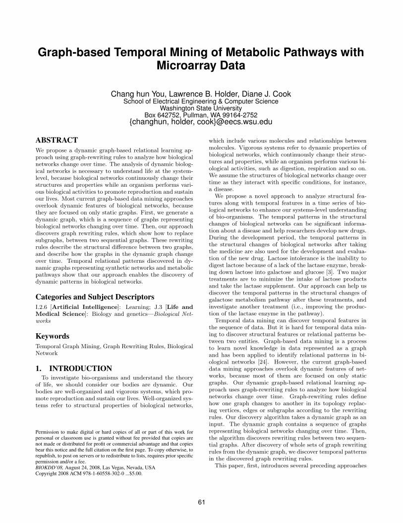
Graph-based Temporal Mining of Metabolic Pathways withMicroarray Data

Chang hun You, Lawrence B. Holder, Diane J. CookSchool of Electrical Engineering & Computer Science

Washington State UniversityBox 642752, Pullman, WA 99164-2752

{changhun, holder, cook}@eecs.wsu.edu

ABSTRACTWe propose a dynamic graph-based relational learning ap-proach using graph-rewriting rules to analyze how biologicalnetworks change over time. The analysis of dynamic biolog-ical networks is necessary to understand life at the system-level, because biological networks continuously change theirstructures and properties while an organism performs vari-ous biological activities to promote reproduction and sustainour lives. Most current graph-based data mining approachesoverlook dynamic features of biological networks, becausethey are focused on only static graphs. First, we generate adynamic graph, which is a sequence of graphs representingbiological networks changing over time. Then, our approachdiscovers graph rewriting rules, which show how to replacesubgraphs, between two sequential graphs. These rewritingrules describe the structural difference between two graphs,and describe how the graphs in the dynamic graph changeover time. Temporal relational patterns discovered in dy-namic graphs representing synthetic networks and metabolicpathways show that our approach enables the discovery ofdynamic patterns in biological networks.

Categories and Subject DescriptorsI.2.6 [Artificial Intelligence]: Learning; J.3 [Life andMedical Science]: Biology and genetics—Biological Net-works

KeywordsTemporal Graph Mining, Graph Rewriting Rules, BiologicalNetwork

1. INTRODUCTIONTo investigate bio-organisms and understand the theory

of life, we should consider our bodies are dynamic. Ourbodies are well-organized and vigorous systems, which pro-mote reproduction and sustain our lives. Well-organized sys-tems refer to structural properties of biological networks,

Permission to make digital or hard copies of all or part of this work forpersonal or classroom use is granted without fee provided that copies arenot made or distributed for profit or commercial advantage and that copiesbear this notice and the full citation on the first page. To copy otherwise, torepublish, to post on servers or to redistribute to lists, requires prior specificpermission and/or a fee.BIOKDD’08, August 24, 2008, Las Vegas, Nevada, USACopyright 2008 ACM 978-1-60558-302-0 ...$5.00.

which include various molecules and relationships betweenmolecules. Vigorous systems refer to dynamic properties ofbiological networks, which continuously change their struc-tures and properties, while an organism performs various bi-ological activities, such as digestion, respiration and so on.We assume the structures of biological networks change overtime as they interact with specific conditions, for instance,a disease.

We propose a novel approach to analyze structural fea-tures along with temporal features in a time series of bio-logical networks to enhance our systems-level understandingof bio-organisms. The temporal patterns in the structuralchanges of biological networks can be significant informa-tion about a disease and help researchers develop new drugs.During the development period, the temporal patterns inthe structural changes of biological networks after takingthe medicine are also used for the development and evalua-tion of the new drug. Lactose intolerance is the inability todigest lactose because of a lack of the lactase enzyme, break-ing down lactose into galactose and glucose [3]. Two majortreatments are to minimize the intake of lactose productsand take the lactase supplement. Our approach can help usdiscover the temporal patterns in the structural changes ofgalactose metabolism pathway after these treatments, andinvestigate another treatment (i.e., improving the produc-tion of the lactase enzyme in the pathway).

Temporal data mining can discover temporal features inthe sequence of data. But it is hard for temporal data min-ing to discover structural features or relational patterns be-tween two entities. Graph-based data mining is a processto learn novel knowledge in data represented as a graphand has been applied to identify relational patterns in bi-ological networks [24]. However, the current graph-baseddata mining approaches overlook dynamic features of net-works, because most of them are focused on only staticgraphs. Our dynamic graph-based relational learning ap-proach uses graph-rewriting rules to analyze how biologicalnetworks change over time. Graph-rewriting rules definehow one graph changes to another in its topology replac-ing vertices, edges or subgraphs according to the rewritingrules. Our discovery algorithm takes a dynamic graph as aninput. The dynamic graph contains a sequence of graphsrepresenting biological networks changing over time. Then,the algorithm discovers rewriting rules between two sequen-tial graphs. After discovery of whole sets of graph rewritingrules from the dynamic graph, we discover temporal patternsin the discovered graph rewriting rules.

This paper, first, introduces several preceding approaches

61

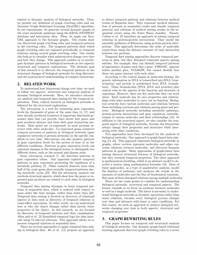
related to dynamic analysis of biological networks. Then,we present our definition of graph rewriting rules and ourDynamic Graph Relational Learning (DynGRL) algorithm.In our experiments, we generate several dynamic graphs ofthe yeast metabolic pathways using the KEGG PATHWAYdatabase and microarray data. Then, we apply our Dyn-GRL approach to the dynamic graphs. The results showour discovered graph rewriting rules and temporal patternsin the rewriting rules. The temporal patterns show whichgraph rewriting rules are repeated periodically or temporalrelations among several graph rewriting rules. Our resultsalso help us to visualize what substructures change over timeand how they change. This approach enables us to investi-gate dynamic patterns in biological networks in two aspects:structural and temporal explorations. The ultimate goalof this research is to discover the temporal patterns in thestructural changes of biological networks for drug discoveryand the systems-level understanding of complex biosystems.

2. RELATED WORKTo understand how biosystems change over time, we need

to follow two aspects: structural and temporal analysis ofdynamic biological networks. Here, we introduce microar-ray analysis and temporal data mining for the temporal ex-ploration. Then, related research on biological networks isfollowed for the structural exploration.

The microarray is a tool for measuring gene expressionlevels for thousands of genes at the same time [4, 17], andhave already produced terabytes of important functional ge-nomics data that can provide clues about how genes andgene products interact and form their gene interaction net-works. Most genes are co-expressed, as most proteins in-teract with other molecules. Co-expressed genes constructcommon processes or patterns in biological networks (generegulatory networks or protein networks) in the specific con-dition or over time. Microarrays can also monitor patternsin gene expression levels for the period of time or at thedifferent conditions. Patterns in gene expression levels canrepresent changes in the biological status or distinguish twodifferent states, such as the normal and disease state.

Some microarray research [7, 22] describes patterns ingene expression values. One approach explores temporalpatterns in gene expression promoting the regulation of ametabolic pathway [7]. Other research observes more thanhalf of the yeast genes show periodic temporal patterns dur-ing metabolic cycles [22]. But the microarray analysis canoverlook structural aspects, which show how the genes or ex-pressed gene products are related to each other in biologicalnetworks.

Temporal data mining attempts to learn temporal pat-terns in sequential data, which is ordered with respect tosome index like time stamps, rather than static data [20].Temporal data mining is focused on discovery of relationalaspects in data such as discovery of temporal relations orcause-effect association. In other words, we can understandhow or why the object changes rather than merely staticproperties of the object. In this research, we are focusedon discovery of temporal patterns and their visualization.Allen and et al. [2] formalized temporal logic for time inter-vals using 13 interval relations. This approach allows us topresent temporal relations in sequential data.

There are several approaches to apply temporal data min-ing in biological data. Ho et al. [11] propose an approach

to detect temporal patterns and relations between medicalevents of Hepatitis data. They represent medical informa-tion of patients as sequential events and classify temporalpatterns and relations of medical testing results in the se-quential events using the Naive Bayes classifier. Farach-Colton et al. [9] introduce an approach of mining temporalrelations in protein-protein interactions. They model theassembly pathways of Ribosome using protein-protein inter-actions. This approach determines the order of molecularconnections using the distance measure of each interactionbetween two proteins.

Temporal data mining approaches discover temporal pat-terns in data, but they disregard relational aspects amongentities. For example, they can identify temporal patternsof appearance of genes such that a gene, YBR218C, appearsbefore another gene, YGL062W, but cannot identify howthese two genes interact with each other.

According to the central dogma in molecular biology, thegenetic information in DNA is transcribed into RNA (tran-scription) and protein is synthesized from RNA (transla-tion). These biomolecules (DNA, RNA and proteins) playcentral roles in the aspects of the function and structure oforganisms. However, there are few molecules that can workalone. Each molecule has its own properties and relation-ships with other molecules to carry out its function. Biolog-ical networks have various molecules and relations betweenthem including reactions and relations among genes and pro-teins. Biological networks including metabolic pathways,protein-protein interactions and gene regulatory networks,consist of various molecules and their relationships [13]. Inaddition to the structural aspect, we also consider the tem-poral aspect of biological networks, because the biosystemsalways change their properties and structures while inter-acting with other conditions.

Two approaches have been developed for the analysis ofbiological networks. One approach is graph-based data min-ing [14, 24]. This approach represents biological networks asgraphs, where vertices represent molecules and edges rep-resent relations between molecules, and discovers frequentpatterns in graphs. Many approaches of graph-based datamining discover structural features of biological networks,but they overlook temporal properties. The other approachis mathematical modeling, which is an abstract model to de-scribe a system using mathematical formulae [18]. Most ofthese approaches, as a type of quantitative analysis, modelthe kinetics of pathways and analyzes the trends in theamounts of molecules and the flux of biochemical reactions.But most of them disregard relations among multiple molecules.

There are two main points to consider for understandingbiological networks: structural and temporal aspects. Theformer reminds us to focus on relations between moleculesas well as a single molecule. The latter is necessary to under-stand biological networks as dynamic operations rather thanstatic relations, because every biological process changesover time and interacts with inner or outer conditions. Forthis reason, we need an approach to analyze biological net-works changing over time in both aspects: structural andtemporal properties.

3. GRAPH REWRITING RULESThis paper focuses on temporal and structural analysis

of biological networks. Our dynamic graph-based relationallearning approach discovers graph rewriting rules in a series

62

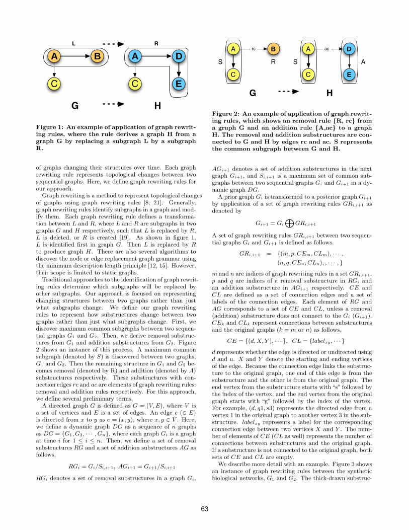
A A

C C

DB

E

L R

G H

Figure 1: An example of application of graph rewrit-ing rules, where the rule derives a graph H from agraph G by replacing a subgraph L by a subgraphR.

of graphs changing their structures over time. Each graphrewriting rule represents topological changes between twosequential graphs. Here, we define graph rewriting rules forour approach.

Graph rewriting is a method to represent topological changesof graphs using graph rewriting rules [8, 21]. Generally,graph rewriting rules identify subgraphs in a graph and mod-ify them. Each graph rewriting rule defines a transforma-tion between L and R, where L and R are subgraphs in twographs G and H respectively, such that L is replaced by R,L is deleted, or R is created [19]. As shown in figure 1,L is identified first in graph G. Then L is replaced by Rto produce graph H. There are also several algorithms todiscover the node or edge replacement graph grammar usingthe minimum description length principle [12, 15]. However,their scope is limited to static graphs.

Traditional approaches to the identification of graph rewrit-ing rules determine which subgraphs will be replaced byother subgraphs. Our approach is focused on representingchanging structures between two graphs rather than justwhat subgraphs change. We define our graph rewritingrules to represent how substructures change between twographs rather than just what subgraphs change. First, wediscover maximum common subgraphs between two sequen-tial graphs G1 and G2. Then, we derive removal substruc-tures from G1 and addition substructures from G2. Figure2 shows an instance of this process. A maximum commonsubgraph (denoted by S) is discovered between two graphs,G1 and G2. Then the remaining structure in G1 and G2 be-comes removal (denoted by R) and addition (denoted by A)substructures respectively. These substructures with con-nection edges rc and ac are elements of graph rewriting rules:removal and addition rules respectively. For this approach,we define several preliminary terms.

A directed graph G is defined as G = (V, E), where V isa set of vertices and E is a set of edges. An edge e (∈ E)is directed from x to y as e = (x, y), where x, y ∈ V . Here,we define a dynamic graph DG as a sequence of n graphsas DG = {G1, G2, · · · , Gn}, where each graph Gi is a graphat time i for 1 ≤ i ≤ n. Then, we define a set of removalsubstructures RG and a set of addition substructures AG asfollows.

RGi = Gi/Si,i+1, AGi+1 = Gi+1/Si,i+1

RGi denotes a set of removal substructures in a graph Gi,

A A

C C

DB

E

G H

rc ac

S AR S

Figure 2: An example of application of graph rewrit-ing rules, which shows an removal rule {R, rc} froma graph G and an addition rule {A,ac} to a graphH. The removal and addition substructures are con-nected to G and H by edges rc and ac. S representsthe common subgraph between G and H.

AGi+1 denotes a set of addition substructures in the nextgraph Gi+1, and Si,i+1 is a maximum set of common sub-graphs between two sequential graphs Gi and Gi+1 in a dy-namic graph DG.

A prior graph Gi is transformed to a posterior graph Gi+1

by application of a set of graph rewriting rules GRi,i+1 asdenoted by

Gi+1 = Gi

MGRi,i+1

A set of graph rewriting rules GRi,i+1 between two sequen-tial graphs Gi and Gi+1 is defined as follows.

GRi,i+1 = {(m, p, CEm, CLm), · · · ,(n, q, CEn, CLn), , · · · , }

m and n are indices of graph rewriting rules in a set GRi,i+1.p and q are indices of a removal substructure in RGi andan addition substructure in AGi+1 respectively. CE andCL are defined as a set of connection edges and a set oflabels of the connection edges. Each element of RG andAG corresponds to a set of CE and CL, unless a removal(addition) substructure does not connect to the Gi (Gi+1).CEk and CLk represent connections between substructuresand the original graphs (k = m or n) as follows.

CE = {(d, X, Y ), · · · }, CL = {labelxy, · · · }

d represents whether the edge is directed or undirected usingd and u. X and Y denote the starting and ending verticesof the edge. Because the connection edge links the substruc-ture to the original graph, one end of this edge is from thesubstructure and the other is from the original graph. Theend vertex from the substructure starts with “s” followed bythe index of the vertex, and the end vertex from the originalgraph starts with “g” followed by the index of the vertex.For example, (d, g1, s3) represents the directed edge from avertex 1 in the original graph to another vertex 3 in the sub-structure. labelxy represents a label for the correspondingconnection edge between two vertices X and Y . The num-ber of elements of CE (CL as well) represents the number ofconnections between substructures and the original graph.If a substructure is not connected to the original graph, bothsets of CE and CL are empty.

We describe more detail with an example. Figure 3 showsan instance of graph rewriting rules between the syntheticbiological networks, G1 and G2. The thick-drawn substruc-

63

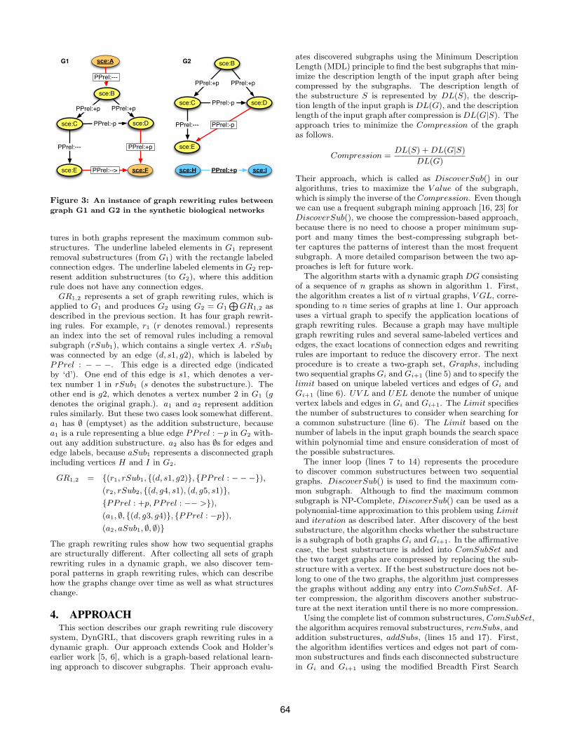
sce:A

sce:B

sce:C sce:D

sce:E sce:F

PPrel:---

PPrel:+p PPrel:+p

PPrel:-p

PPrel:--- PPrel:+p

PPrel:-->

sce:B

sce:C sce:D

sce:E

sce:H sce:I

PPrel:+p PPrel:+p

PPrel:-p

PPrel:--- PPrel:-p

PPrel:+p

G1 G2

Figure 3: An instance of graph rewriting rules between

graph G1 and G2 in the synthetic biological networks

tures in both graphs represent the maximum common sub-structures. The underline labeled elements in G1 representremoval substructures (from G1) with the rectangle labeledconnection edges. The underline labeled elements in G2 rep-resent addition substructures (to G2), where this additionrule does not have any connection edges.

GR1,2 represents a set of graph rewriting rules, which isapplied to G1 and produces G2 using G2 = G1

LGR1,2 as

described in the previous section. It has four graph rewrit-ing rules. For example, r1 (r denotes removal.) representsan index into the set of removal rules including a removalsubgraph (rSub1), which contains a single vertex A. rSub1

was connected by an edge (d, s1, g2), which is labeled byPPrel : − − −. This edge is a directed edge (indicatedby ‘d’). One end of this edge is s1, which denotes a ver-tex number 1 in rSub1 (s denotes the substructure.). Theother end is g2, which denotes a vertex number 2 in G1 (gdenotes the original graph.). a1 and a2 represent additionrules similarly. But these two cases look somewhat different.a1 has ∅ (emptyset) as the addition substructure, becausea1 is a rule representing a blue edge PPrel : −p in G2 with-out any addition substructure. a2 also has ∅s for edges andedge labels, because aSub1 represents a disconnected graphincluding vertices H and I in G2.

GR1,2 = {(r1, rSub1, {(d, s1, g2)}, {PPrel : −−−}),(r2, rSub2, {(d, g4, s1), (d, g5, s1)},{PPrel : +p, PPrel : −− >}),(a1, ∅, {(d, g3, g4)}, {PPrel : −p}),(a2, aSub1, ∅, ∅)}

The graph rewriting rules show how two sequential graphsare structurally different. After collecting all sets of graphrewriting rules in a dynamic graph, we also discover tem-poral patterns in graph rewriting rules, which can describehow the graphs change over time as well as what structureschange.

4. APPROACHThis section describes our graph rewriting rule discovery

system, DynGRL, that discovers graph rewriting rules in adynamic graph. Our approach extends Cook and Holder’searlier work [5, 6], which is a graph-based relational learn-ing approach to discover subgraphs. Their approach evalu-

ates discovered subgraphs using the Minimum DescriptionLength (MDL) principle to find the best subgraphs that min-imize the description length of the input graph after beingcompressed by the subgraphs. The description length ofthe substructure S is represented by DL(S), the descrip-tion length of the input graph is DL(G), and the descriptionlength of the input graph after compression is DL(G|S). Theapproach tries to minimize the Compression of the graphas follows.

Compression =DL(S) + DL(G|S)

DL(G)

Their approach, which is called as DiscoverSub() in ouralgorithms, tries to maximize the V alue of the subgraph,which is simply the inverse of the Compression. Even thoughwe can use a frequent subgraph mining approach [16, 23] forDiscoverSub(), we choose the compression-based approach,because there is no need to choose a proper minimum sup-port and many times the best-compressing subgraph bet-ter captures the patterns of interest than the most frequentsubgraph. A more detailed comparison between the two ap-proaches is left for future work.

The algorithm starts with a dynamic graph DG consistingof a sequence of n graphs as shown in algorithm 1. First,the algorithm creates a list of n virtual graphs, V GL, corre-sponding to n time series of graphs at line 1. Our approachuses a virtual graph to specify the application locations ofgraph rewriting rules. Because a graph may have multiplegraph rewriting rules and several same-labeled vertices andedges, the exact locations of connection edges and rewritingrules are important to reduce the discovery error. The nextprocedure is to create a two-graph set, Graphs, includingtwo sequential graphs Gi and Gi+1 (line 5) and to specify thelimit based on unique labeled vertices and edges of Gi andGi+1 (line 6). UV L and UEL denote the number of uniquevertex labels and edges in Gi and Gi+1. The Limit specifiesthe number of substructures to consider when searching fora common substructure (line 6). The Limit based on thenumber of labels in the input graph bounds the search spacewithin polynomial time and ensure consideration of most ofthe possible substructures.

The inner loop (lines 7 to 14) represents the procedureto discover common substructures between two sequentialgraphs. DiscoverSub() is used to find the maximum com-mon subgraph. Although to find the maximum commonsubgraph is NP-Complete, DiscoverSub() can be used as apolynomial-time approximation to this problem using Limitand iteration as described later. After discovery of the bestsubstructure, the algorithm checks whether the substructureis a subgraph of both graphs Gi and Gi+1. In the affirmativecase, the best substructure is added into ComSubSet andthe two target graphs are compressed by replacing the sub-structure with a vertex. If the best substructure does not be-long to one of the two graphs, the algorithm just compressesthe graphs without adding any entry into ComSubSet. Af-ter compression, the algorithm discovers another substruc-ture at the next iteration until there is no more compression.

Using the complete list of common substructures, ComSubSet,the algorithm acquires removal substructures, remSubs, andaddition substructures, addSubs, (lines 15 and 17). First,the algorithm identifies vertices and edges not part of com-mon substructures and finds each disconnected substructurein Gi and Gi+1 using the modified Breadth First Search

64

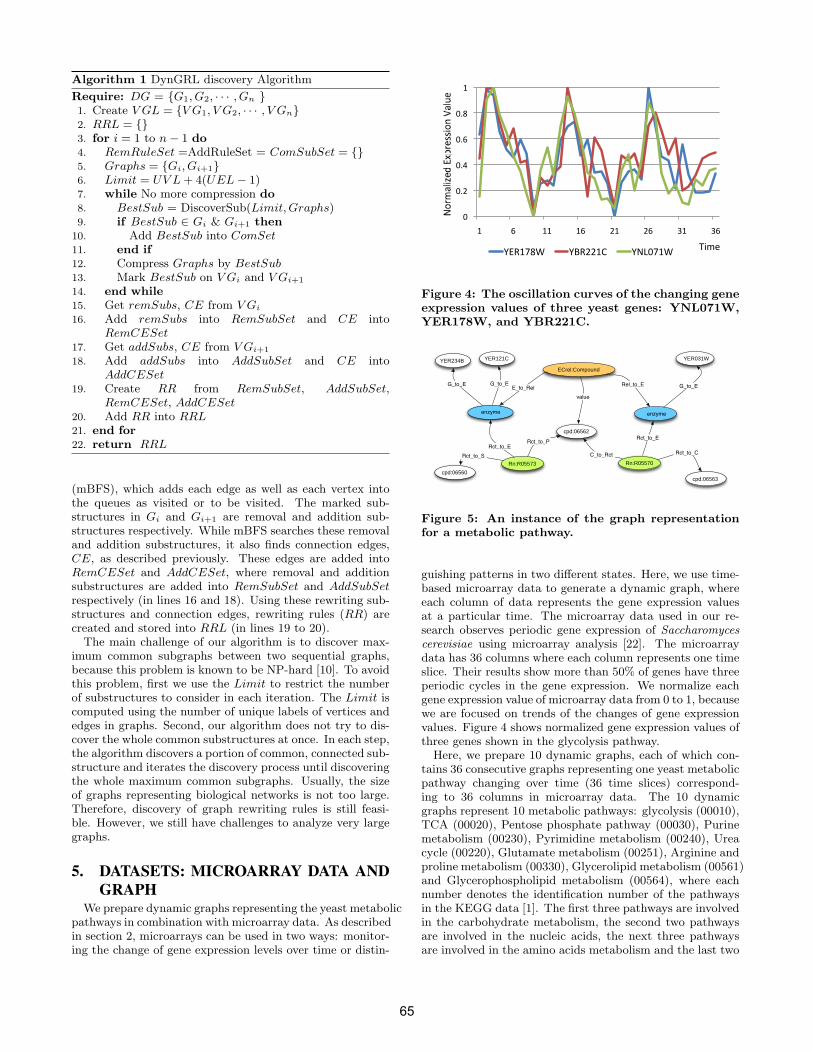
Algorithm 1 DynGRL discovery Algorithm

Require: DG = {G1, G2, · · · , Gn }1. Create V GL = {V G1, V G2, · · · , V Gn}2. RRL = {}3. for i = 1 to n− 1 do4. RemRuleSet =AddRuleSet = ComSubSet = {}5. Graphs = {Gi, Gi+1}6. Limit = UV L + 4(UEL− 1)7. while No more compression do8. BestSub = DiscoverSub(Limit, Graphs)9. if BestSub ∈ Gi & Gi+1 then

10. Add BestSub into ComSet11. end if12. Compress Graphs by BestSub13. Mark BestSub on V Gi and V Gi+1

14. end while15. Get remSubs, CE from V Gi

16. Add remSubs into RemSubSet and CE intoRemCESet

17. Get addSubs, CE from V Gi+1

18. Add addSubs into AddSubSet and CE intoAddCESet

19. Create RR from RemSubSet, AddSubSet,RemCESet, AddCESet

20. Add RR into RRL21. end for22. return RRL

(mBFS), which adds each edge as well as each vertex intothe queues as visited or to be visited. The marked sub-structures in Gi and Gi+1 are removal and addition sub-structures respectively. While mBFS searches these removaland addition substructures, it also finds connection edges,CE, as described previously. These edges are added intoRemCESet and AddCESet, where removal and additionsubstructures are added into RemSubSet and AddSubSetrespectively (in lines 16 and 18). Using these rewriting sub-structures and connection edges, rewriting rules (RR) arecreated and stored into RRL (in lines 19 to 20).

The main challenge of our algorithm is to discover max-imum common subgraphs between two sequential graphs,because this problem is known to be NP-hard [10]. To avoidthis problem, first we use the Limit to restrict the numberof substructures to consider in each iteration. The Limit iscomputed using the number of unique labels of vertices andedges in graphs. Second, our algorithm does not try to dis-cover the whole common substructures at once. In each step,the algorithm discovers a portion of common, connected sub-structure and iterates the discovery process until discoveringthe whole maximum common subgraphs. Usually, the sizeof graphs representing biological networks is not too large.Therefore, discovery of graph rewriting rules is still feasi-ble. However, we still have challenges to analyze very largegraphs.

5. DATASETS: MICROARRAY DATA ANDGRAPH

We prepare dynamic graphs representing the yeast metabolicpathways in combination with microarray data. As describedin section 2, microarrays can be used in two ways: monitor-ing the change of gene expression levels over time or distin-

!"

!#$"

!#%"

!#&"

!#'"

("

(" &" ((" (&" $(" $&" )(" )&"

*+,(-'." */,$$(0" *12!-(."3456"

Figure 4: The oscillation curves of the changing geneexpression values of three yeast genes: YNL071W,YER178W, and YBR221C.

enzyme

YER031W

enzyme

YER234B

ECrel:Compound

cpd:06563cpd:06560

cpd:06562

Rn:R05573 Rn:R05570

value

Rct_to_E

Rct_to_CC_to_Rct

Rct_to_P

E_to_Rel Rel_to_E

Rct_to_SRct_to_E

G_to_E G_to_E G_to_E

YER121C

Figure 5: An instance of the graph representationfor a metabolic pathway.

guishing patterns in two different states. Here, we use time-based microarray data to generate a dynamic graph, whereeach column of data represents the gene expression valuesat a particular time. The microarray data used in our re-search observes periodic gene expression of Saccharomycescerevisiae using microarray analysis [22]. The microarraydata has 36 columns where each column represents one timeslice. Their results show more than 50% of genes have threeperiodic cycles in the gene expression. We normalize eachgene expression value of microarray data from 0 to 1, becausewe are focused on trends of the changes of gene expressionvalues. Figure 4 shows normalized gene expression values ofthree genes shown in the glycolysis pathway.

Here, we prepare 10 dynamic graphs, each of which con-tains 36 consecutive graphs representing one yeast metabolicpathway changing over time (36 time slices) correspond-ing to 36 columns in microarray data. The 10 dynamicgraphs represent 10 metabolic pathways: glycolysis (00010),TCA (00020), Pentose phosphate pathway (00030), Purinemetabolism (00230), Pyrimidine metabolism (00240), Ureacycle (00220), Glutamate metabolism (00251), Arginine andproline metabolism (00330), Glycerolipid metabolism (00561)and Glycerophospholipid metabolism (00564), where eachnumber denotes the identification number of the pathwaysin the KEGG data [1]. The first three pathways are involvedin the carbohydrate metabolism, the second two pathwaysare involved in the nucleic acids, the next three pathwaysare involved in the amino acids metabolism and the last two

65

!" #!" $!" %!"

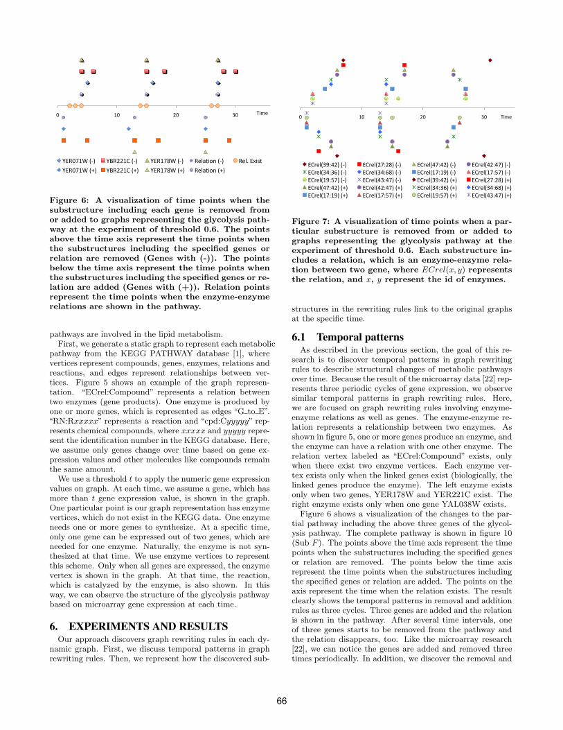
&'(!)#*"+,-" &.($$#/"+,-" &'(#)0*"+,-" (1234567"+,-" (128"'95:4"

&'(!)#*"+;-" &.($$#/"+;-" &'(#)0*"+;-" (1234567"+;-"

<5=1"

Figure 6: A visualization of time points when thesubstructure including each gene is removed fromor added to graphs representing the glycolysis path-way at the experiment of threshold 0.6. The pointsabove the time axis represent the time points whenthe substructures including the specified genes orrelation are removed (Genes with (-)). The pointsbelow the time axis represent the time points whenthe substructures including the specified genes or re-lation are added (Genes with (+)). Relation pointsrepresent the time points when the enzyme-enzymerelations are shown in the pathway.

pathways are involved in the lipid metabolism.First, we generate a static graph to represent each metabolic

pathway from the KEGG PATHWAY database [1], wherevertices represent compounds, genes, enzymes, relations andreactions, and edges represent relationships between ver-tices. Figure 5 shows an example of the graph represen-tation. “ECrel:Compound” represents a relation betweentwo enzymes (gene products). One enzyme is produced byone or more genes, which is represented as edges “G to E”.“RN:Rxxxxx” represents a reaction and “cpd:Cyyyyy” rep-resents chemical compounds, where xxxxx and yyyyy repre-sent the identification number in the KEGG database. Here,we assume only genes change over time based on gene ex-pression values and other molecules like compounds remainthe same amount.

We use a threshold t to apply the numeric gene expressionvalues on graph. At each time, we assume a gene, which hasmore than t gene expression value, is shown in the graph.One particular point is our graph representation has enzymevertices, which do not exist in the KEGG data. One enzymeneeds one or more genes to synthesize. At a specific time,only one gene can be expressed out of two genes, which areneeded for one enzyme. Naturally, the enzyme is not syn-thesized at that time. We use enzyme vertices to representthis scheme. Only when all genes are expressed, the enzymevertex is shown in the graph. At that time, the reaction,which is catalyzed by the enzyme, is also shown. In thisway, we can observe the structure of the glycolysis pathwaybased on microarray gene expression at each time.

6. EXPERIMENTS AND RESULTSOur approach discovers graph rewriting rules in each dy-

namic graph. First, we discuss temporal patterns in graphrewriting rules. Then, we represent how the discovered sub-

!" #!" $!" %!"

&'()*+%,-.$/"+0/" &'()*+$1-$2/"+0/" &'()*+.1-.$/"+0/" &'()*+.$-.1/"+0/"

&'()*+%.-%3/"+0/" &'()*+%.-32/"+0/" &'()*+#1-#,/"+0/" &'()*+#1-41/"+0/"

&'()*+#,-41/"+0/" &'()*+.%-.1/"+0/" &'()*+%,-.$/"+5/" &'()*+$1-$2/"+5/"

&'()*+.1-.$/"+5/" &'()*+.$-.1/"+5/" &'()*+%.-%3/"+5/" &'()*+%.-32/"+5/"

&'()*+#1-#,/"+5/" &'()*+#1-41/"+5/" &'()*+#,-41/"+5/" &'()*+.%-.1/"+5/"

678)"

Figure 7: A visualization of time points when a par-ticular substructure is removed from or added tographs representing the glycolysis pathway at theexperiment of threshold 0.6. Each substructure in-cludes a relation, which is an enzyme-enzyme rela-tion between two gene, where ECrel(x, y) representsthe relation, and x, y represent the id of enzymes.

structures in the rewriting rules link to the original graphsat the specific time.

6.1 Temporal patternsAs described in the previous section, the goal of this re-

search is to discover temporal patterns in graph rewritingrules to describe structural changes of metabolic pathwaysover time. Because the result of the microarray data [22] rep-resents three periodic cycles of gene expression, we observesimilar temporal patterns in graph rewriting rules. Here,we are focused on graph rewriting rules involving enzyme-enzyme relations as well as genes. The enzyme-enzyme re-lation represents a relationship between two enzymes. Asshown in figure 5, one or more genes produce an enzyme, andthe enzyme can have a relation with one other enzyme. Therelation vertex labeled as “ECrel:Compound” exists, onlywhen there exist two enzyme vertices. Each enzyme ver-tex exists only when the linked genes exist (biologically, thelinked genes produce the enzyme). The left enzyme existsonly when two genes, YER178W and YER221C exist. Theright enzyme exists only when one gene YAL038W exists.

Figure 6 shows a visualization of the changes to the par-tial pathway including the above three genes of the glycol-ysis pathway. The complete pathway is shown in figure 10(Sub F ). The points above the time axis represent the timepoints when the substructures including the specified genesor relation are removed. The points below the time axisrepresent the time points when the substructures includingthe specified genes or relation are added. The points on theaxis represent the time when the relation exists. The resultclearly shows the temporal patterns in removal and additionrules as three cycles. Three genes are added and the relationis shown in the pathway. After several time intervals, oneof three genes starts to be removed from the pathway andthe relation disappears, too. Like the microarray research[22], we can notice the genes are added and removed threetimes periodically. In addition, we discover the removal and

66

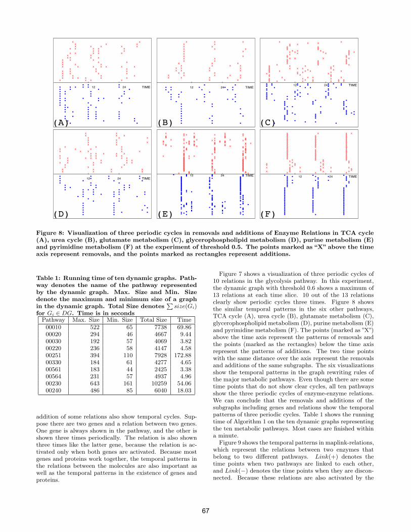
(A) (B) (C)

(D) (E) (F)

X X

| |

12 24 TIME

X X X

X X X X X

X X X X X

X X X

X X X X X

X X

X X X X

X X X

X X X

X X X

X X X X X X X

X X X

X X X X

X X X X

X X X X

X X X X X X

X X X X

X X X

| |

12 24 TIME

X X

X X

X X X

X X

X

X X

X X

X X

X X X

X X X X

X X X X

X X X X

X X X

X X X X X

X X X X X

X X

X X

| |

12 24 TIME

X XX XX

X XX XX X

X X X XX X X X X

X X XX X

X XX XX X X X

X XX X XX X XX X X

X X XX X X XX XX X X X XX X XX X X X XX X X X

X X XX X XX X

X X X XX X XX X X X X XX X X X X X X

X X

| |

12 24 TIME

X X X

X X X

X X

X X X

X X

X X X

X X X

X X X X X

X X X X X

X X X X X

X X X X X X X

X

X

X X X

X X X X X X

X X X

X X X

X X X X

X X X X

X X X

| |12 24 TIME

X XX X XX XX X XX X XX X XX XXX

XX X X XX X XX X X X XX X X X XX X XX X X X XX X X X XX X XX X XX X X XX XX X XX X XX X XX X XX X XX XX XX XX XX X XX XX XX X XX X XX XX X X XX XX X XX X XX X XX XX XX X XX X XX XX XX X XX X XX X XX XX X XX X XX X XX XX X XX X XX X X X

X X X

| |

12 24 TIME

X XX X XX X XX X XX X XX X XX X XX X XX X XX X XX X XX XX X XX X XX X XX X XX X XX X XX X XX X X

X X X XX X XX X X

X X XX X X X

X X

X

X X X X X XX X XX X X

X X X X X XX X X

Figure 8: Visualization of three periodic cycles in removals and additions of Enzyme Relations in TCA cycle(A), urea cycle (B), glutamate metabolism (C), glycerophospholipid metabolism (D), purine metabolism (E)and pyrimidine metabolism (F) at the experiment of threshold 0.5. The points marked as “X” above the timeaxis represent removals, and the points marked as rectangles represent additions.

Table 1: Running time of ten dynamic graphs. Path-way denotes the name of the pathway representedby the dynamic graph. Max. Size and Min. Sizedenote the maximum and minimum size of a graphin the dynamic graph. Total Size denotes

Psize(Gi)

for Gi ∈ DG. Time is in secondsPathway Max. Size Min. Size Total Size Time

00010 522 65 7738 69.8600020 294 46 4667 9.4400030 192 57 4069 3.8200220 236 58 4147 4.5800251 394 110 7928 172.8800330 184 61 4277 4.6500561 183 44 2425 3.3800564 231 57 4937 4.9600230 643 161 10259 54.0600240 486 85 6040 18.03

addition of some relations also show temporal cycles. Sup-pose there are two genes and a relation between two genes.One gene is always shown in the pathway, and the other isshown three times periodically. The relation is also shownthree times like the latter gene, because the relation is ac-tivated only when both genes are activated. Because mostgenes and proteins work together, the temporal patterns inthe relations between the molecules are also important aswell as the temporal patterns in the existence of genes andproteins.

Figure 7 shows a visualization of three periodic cycles of10 relations in the glycolysis pathway. In this experiment,the dynamic graph with threshold 0.6 shows a maximum of13 relations at each time slice. 10 out of the 13 relationsclearly show periodic cycles three times. Figure 8 showsthe similar temporal patterns in the six other pathways,TCA cycle (A), urea cycle (B), glutamate metabolism (C),glycerophospholipid metabolism (D), purine metabolism (E)and pyrimidine metabolism (F). The points (marked as ”X”)above the time axis represent the patterns of removals andthe points (marked as the rectangles) below the time axisrepresent the patterns of additions. The two time pointswith the same distance over the axis represent the removalsand additions of the same subgraphs. The six visualizationsshow the temporal patterns in the graph rewriting rules ofthe major metabolic pathways. Even though there are sometime points that do not show clear cycles, all ten pathwaysshow the three periodic cycles of enzyme-enzyme relations.We can conclude that the removals and additions of thesubgraphs including genes and relations show the temporalpatterns of three periodic cycles. Table 1 shows the runningtime of Algorithm 1 on the ten dynamic graphs representingthe ten metabolic pathways. Most cases are finished withina minute.

Figure 9 shows the temporal patterns in maplink-relations,which represent the relations between two enzymes thatbelong to two different pathways. Link(+) denotes thetime points when two pathways are linked to each other,and Link(−) denotes the time points when they are discon-nected. Because these relations are also activated by the

67

!" #$" $%"

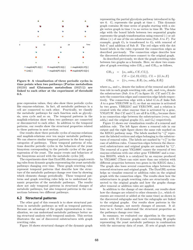
&'()*+,-.#/01234" &'()*+,-.$/01234" &'()*+,-0#/.1234"

5*+,234" &'()*+,-.#/01264" &'()*+,-.$/01264"

7*&8"

Figure 9: A visualization of three periodic cycles intime points when two pathways (Purine metabolism(00230) and Glutamate metabolism (00251)) arelinked to each other at the experiment of threshold0.5.

gene expression values, they also show three periodic cycleslike enzyme-relations. In fact, all metabolic pathways in acell are connected to each other. Practically, we classifythe metabolic pathways for each function such as glycoly-sis, urea cycle and so on. The temporal patterns in themaplink-relations show when two pathways are connectedor disconnected to each other. In addition to the temporalpatterns, our results show the structural properties relatedto these patterns in next section.

Our results show three periodic cycles of enzyme-relationsand maplink-relations over ten major metabolic pathways.We can observe similar temporal patterns in the four majorcategories of pathways. These temporal patterns of rela-tions describe periodic cycles in the behaviors of the yeastbiosystem corresponding to the periodic cycles of the geneexpression of the yeast. The major events and behaviors ofthe biosystems accord with the metabolic cycles [22].

The experiments show that DynGRL discovers graph rewrit-ing rules from dynamic graphs representing the yeast metabolicpathways changing over time. These graph rewriting rulesrepresent temporal patterns that describe how the struc-ture of the metabolic pathways change over time by showingwhich elements change periodically. These temporal pat-terns and graph rewriting rules help us to understand dy-namic properties of the metabolic pathways. The resultsshow not only temporal patterns in structural changes ofmetabolic pathways, but also temporal patterns in the con-nections between two different pathways.

6.2 Structural patternsThe other goal of this research is to show structural pat-

terns in metabolic pathways as well as temporal patterns.Because an advantage of the graph representation is visu-alization, we can understand metabolic pathways better us-ing structural analysis with temporal analysis. This sectionillustrates the use of discovered substructures with graphrewriting rules.

Figure 10 shows structural changes of the dynamic graph

representing the partial glycolysis pathway introduced in fig-ure 6. Gi represents the graph at time i. This dynamicgraph contains 36 time series of graphs starting with a sin-gle vertex graph in time 1 to no vertex in time 36. The blueedge with the boxed labels between two sequential graphsrepresents the graph transformation using removal (-) or ad-dition (+) of one of the six substructures (Sub A to F ). Forexample, graph G5 is transformed to G6 with removal ofSub C and addition of Sub B. The red edges with the dotboxed labels in the rules represent the connection edges asdescribed previously. The connection edges describe howthe discovered substructures connect to the original graph.

As described previously, we show the graph rewriting rulesbetween two graphs as a formula. Here, we show two exam-ples of graph rewriting rules GR1,2 and GR5,6 as follows,

GR1,2 = {a1, addA, CE, CL)},CE = {(d, S2, G2)}, CL = {G to E}

GR5,6 = {(r1, remC , ∅, ∅), (a1, addB , ∅, ∅)}

where am and rn denote the indices of the removal and addi-tion rule in each graph rewriting rule, addx and remy denotethe substructure (Sub A to F ) in figure 10. CE and CL de-note the connection edges and connection edge labels respec-tively. The connection edge with a label G to E links SubA to a gene YER178W in G1 so that an enzyme is activatedby two genes, YBR221C and YER178W, and a relation iscreated with the other enzyme that is activated by a gene,YNL071W. But CE and CL are all ∅ in GR5,6 because thereis no connection edge between the substructures (remC andaddB) and the original graphs (G5 and G6) respectively.

Figure 11 shows our visualization results of a removal andaddition rule. The left figure shows a removal rule in ouroutput and the right figure shows the same rule marked onthe KEGG pathway map. The labels marked by “-[]” repre-sent the labeled vertices and edges belonging to the substruc-tures of removal rules. The labels are marked by “+[]” in thecase of addition rules. Connection edges between the discov-ered substructures and original graphs are marked by “()”.The removal of a gene YKL060C causes the removal of twoenzyme-relations with one other gene YDR050C and a reac-tion R01070, which is a catalyzed by an enzyme producedby YKL060C (There can exist more than one relation withdifferent properties between two genes in the KEGG data.).The graph also loses several connection edges between theremoval structures and original graph. The DynGRL systemhelps us visualize removal or addition rules on the originalgraph with the connection edges. The results show how thesubstructures in graph rewriting rules are structurally con-nected to the original graphs and how the graphs changeafter removal or addition rules are applied.

In addition to the change of one element, our results showhow the changes are related to other elements (i.e., which el-ements are removed or added at the same time) as shown inthe discovered subgraphs and how the subgraphs are linkedto the original graphs. Our results show patterns in thestructural changes, not merely changes of amount. It al-lows us to better understand the structural properties asthe pathways change over time.

In summary, we evaluated our algorithm in the experi-ments with 10 dynamic graphs each containing 36 graphsrepresenting the yeast metabolic pathways in combinationwith the microarray data of yeast. 35 sets of graph rewrit-

68

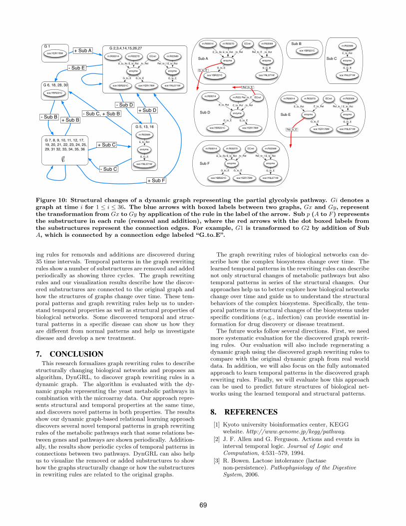
sce:YER178W

G 1 G 2,3,4,14,15,26,27

sce:YBR221C sce:YER178W

enzyme

sce:YNL071W

enzyme

ECrel:rn:R00014 rn:R03270 rn:R02569

G_to_E G_to_E G_to_E

E_to_Rel Rel_to_EE_to_RctE_to_Rct E_to_Rct

sce:YBR221C

G 6, 18, 28, 30

∅

G 7, 8, 9, 10, 11, 12, 17, 19, 20, 21, 22, 23, 24, 25, 29, 31 32, 33, 34, 35, 36

sce:YNL071W

enzyme

rn:R02569

G_to_E

E_to_Rct

G 5, 13, 16

G_to_E

E_to_Rct

sce:YBR221C

enzyme

sce:YNL071W

enzyme

rn:R00014 rn:R03270 rn:R02569

G_to_EG_to_E

E_to_Rel Rel_to_EE_to_RctE_to_Rct

ECrel:

Sub A

sce:YBR221C

Sub B

sce:YNL071W

enzyme

rn:R02569

G_to_E

E_to_Rct

Sub C

sce:YER178W

enzyme

sce:YNL071W

enzyme

ECrel:rn:R00014 rn:R03270 rn:R02569

G_to_E

E_to_Rel Rel_to_EE_to_Rct E_to_Rct

G_to_E

Rel_to_E

Sub E

+ Sub A

- Sub D- Sub C, + Sub B- Sub B

+ Sub C

+ Sub D

- Sub C

+ Sub B

sce:YBR221C sce:YER178W

enzyme

sce:YNL071W

enzyme

ECrel:rn:R00014 rn:R03270 rn:R02569

G_to_E G_to_E G_to_E

E_to_Rel Rel_to_EE_to_RctE_to_Rct E_to_Rct

Sub F

+ Sub F

- Sub E

rn:R00014

E_to_Rct

sce:YBR221C

G_to_E

sce:YER178W

enzyme

ECrel:rn:R03270

G_to_E

E_to_RelE_to_Rct

Sub D

Rel_to_E

Rel_to_E

Figure 10: Structural changes of a dynamic graph representing the partial glycolysis pathway. Gi denotes agraph at time i for 1 ≤ i ≤ 36. The blue arrows with boxed labels between two graphs, Gx and Gy, representthe transformation from Gx to Gy by application of the rule in the label of the arrow. Sub p (A to F ) representsthe substructure in each rule (removal and addition), where the red arrows with the dot boxed labels fromthe substructures represent the connection edges. For example, G1 is transformed to G2 by addition of SubA, which is connected by a connection edge labeled “G to E”.

ing rules for removals and additions are discovered during35 time intervals. Temporal patterns in the graph rewritingrules show a number of substructures are removed and addedperiodically as showing three cycles. The graph rewritingrules and our visualization results describe how the discov-ered substructures are connected to the original graph andhow the structures of graphs change over time. These tem-poral patterns and graph rewriting rules help us to under-stand temporal properties as well as structural properties ofbiological networks. Some discovered temporal and struc-tural patterns in a specific disease can show us how theyare different from normal patterns and help us investigatedisease and develop a new treatment.

7. CONCLUSIONThis research formalizes graph rewriting rules to describe

structurally changing biological networks and proposes analgorithm, DynGRL, to discover graph rewriting rules in adynamic graph. The algorithm is evaluated with the dy-namic graphs representing the yeast metabolic pathways incombination with the microarray data. Our approach repre-sents structural and temporal properties at the same time,and discovers novel patterns in both properties. The resultsshow our dynamic graph-based relational learning approachdiscovers several novel temporal patterns in graph rewritingrules of the metabolic pathways such that some relations be-tween genes and pathways are shown periodically. Addition-ally, the results show periodic cycles of temporal patterns inconnections between two pathways. DynGRL can also helpus to visualize the removed or added substructures to showhow the graphs structurally change or how the substructuresin rewriting rules are related to the original graphs.

The graph rewriting rules of biological networks can de-scribe how the complex biosystems change over time. Thelearned temporal patterns in the rewriting rules can describenot only structural changes of metabolic pathways but alsotemporal patterns in series of the structural changes. Ourapproaches help us to better explore how biological networkschange over time and guide us to understand the structuralbehaviors of the complex biosystems. Specifically, the tem-poral patterns in structural changes of the biosystems underspecific conditions (e.g., infection) can provide essential in-formation for drug discovery or disease treatment.

The future works follow several directions. First, we needmore systematic evaluation for the discovered graph rewrit-ing rules. Our evaluation will also include regenerating adynamic graph using the discovered graph rewriting rules tocompare with the original dynamic graph from real worlddata. In addition, we will also focus on the fully automatedapproach to learn temporal patterns in the discovered graphrewriting rules. Finally, we will evaluate how this approachcan be used to predict future structures of biological net-works using the learned temporal and structural patterns.

8. REFERENCES[1] Kyoto university bioinformatics center, KEGG

website. http://www.genome.jp/kegg/pathway.

[2] J. F. Allen and G. Ferguson. Actions and events ininterval temporal logic. Journal of Logic andComputation, 4:531–579, 1994.

[3] R. Bowen. Lactose intolerance (lactasenon-persistence). Pathophysiology of the DigestiveSystem, 2006.

69

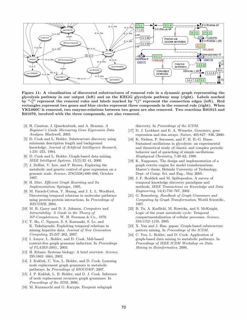
5/25/08 5:20 AMKEGG PATHWAY: Glycolysis / Gluconeogenesis - Saccharomyces cerevisiae S288C

Page 1 of 2http://www.genome.jp/dbget-bin/show_pathway?sce00010+ykl060c

Glycolysis / Gluconeogenesis - Saccharomyces cerevisiae S288C

[ Pathway menu | Ortholog table ]

Saccharomyces cerevisiae Go Current selection

sce:YOR374W sce:YPL061W sce:YAL054C sce:YMR170C cpd:C00033

path:sce00650path:sce00660

path:sce00640 path:sce00710

path:sce00030-[path:sce00500] -[path:sce00040]

sce:YDR380W -[sce:YLR044C] sce:YMR303C -[sce:YOL086C]

sce:YBR221C sce:YER178W

enzyme

sce:YNL071W

enzyme path:sce00072

path:sce00620

path:sce00020

path:sce00010 -[sce:YMR323W]

path:sce00561path:sce00052

sce:YJL052W

path:sce00710

sce:YDR050C

enzyme

path:sce00051

-[sce:YKL060C]

enzyme

-[sce:YKL127W] -[sce:YMR105C]

enzyme -[path:sce00052]

sce:YFR053C

sce:YCL040W

enzyme

path:sce00010

-[sce:YFL018C] -[sce:YPL017C]

-[enzyme]-[path:sce00520] path:sce00730 path:sce00770

path:sce00400

path:sce00350path:sce00380

path:sce00440

path:sce00252path:sce00300 path:map00473

sce:YCR012W

-[enzyme]

cpd:C00031

-[cpd:C00103]

cpd:C00631

cpd:C00267 cpd:C00221

cpd:C00111

cpd:C01172cpd:C00668

cpd:C00118

-[cpd:C05345] cpd:C00074

cpd:C00197 cpd:C00236

cpd:C00186 cpd:C01159

cpd:C15972

cpd:C00469

cpd:C00022 cpd:C05125 cpd:C00068cpd:C00024

cpd:C00084

cpd:C16255 cpd:C15973

cpd:C05378

cpd:C02827 cpd:C06189 cpd:C06186 cpd:C06187 cpd:C06188 cpd:C01451 -[ECrel:compound]

-[ECrel:compound]

-[ECrel:compound]

ECrel:compound -[ECrel:compound]-[ECrel:compound]-[maplink:compound] -[maplink:compound] -[maplink:compound] -[maplink:compound] maplink:compound -[maplink:compound]-[maplink:compound] -[maplink:compound] -[maplink:compound] -[maplink:compound]maplink:compoundmaplink:compound maplink:compound maplink:compound maplink:compound maplink:compound maplink:compound maplink:compound maplink:compoundmaplink:compoundmaplink:compound -[maplink:compound] maplink:compound maplink:compound maplink:compound maplink:compound maplink:compound maplink:compound maplink:compound maplink:compoundmaplink:compoundmaplink:compound rn:R00014rn:R03270rn:R02569

rn:R01015

-[rn:R01070]

-[rn:R00959] rn:R01600rn:R01786 -[rn:R07618] rn:R01512

G_to_E G_to_EG_to_E

G_to_E

(G_to_E)

(G_to_E) (G_to_E) G_to_E -[G_to_E] -[G_to_E] G_to_E

(value)(E_to_Rel) (Rel_to_E)

(value)

(E_to_Rel)

(Rel_to_E)

(value)

(E_to_Rel) (Rel_to_E)

value E_to_RelRel_to_E (value) (E_to_Rel)-[Rel_to_E](value)(E_to_Rel) -[Rel_to_E]-[value] (E_to_Rel)-[Rel_to_E] -[value] (E_to_Rel)-[Rel_to_E] -[value] (E_to_Rel)-[Rel_to_E] (value)(E_to_Rel)-[Rel_to_E] (value)E_to_Rel (Rel_to_E)

(value)

(E_to_Rel)

(Rel_to_E)

(value)

(E_to_Rel)

(Rel_to_E)

(value)

(E_to_Rel)

(Rel_to_E)

(value)

(E_to_Rel)

(Rel_to_E)

(value)

(E_to_Rel)

(Rel_to_E)

value

E_to_Rel

Rel_to_E

value

E_to_Rel

Rel_to_E

value

E_to_Rel

Rel_to_E

value

E_to_Rel

Rel_to_E

value

E_to_Rel

Rel_to_E value E_to_RelRel_to_E value E_to_RelRel_to_E value E_to_Rel Rel_to_Evalue E_to_Rel Rel_to_Evalue E_to_Rel Rel_to_Evalue E_to_Rel(Rel_to_E) value-[E_to_Rel]Rel_to_E valueE_to_RelRel_to_E valueE_to_RelRel_to_E valueE_to_Rel Rel_to_E valueE_to_Rel Rel_to_E valueE_to_Rel Rel_to_EvalueE_to_Rel Rel_to_EvalueE_to_Rel Rel_to_EvalueE_to_Rel Rel_to_E

value

E_to_Rel

Rel_to_E

(value)

E_to_Rel

Rel_to_E E_to_Rct S_to_RctS_to_Rct Rct_to_PE_to_RctS_to_Rct S_to_Rct Rct_to_PRct_to_PE_to_Rct C_to_RctC_to_Rct Rct_to_C

E_to_Rct

C_to_Rct

Rct_to_C

(E_to_Rct)

(C_to_Rct)

(Rct_to_C)

(Rct_to_C)

(E_to_Rct)-[C_to_Rct] (Rct_to_C) E_to_Rct C_to_Rct Rct_to_CE_to_Rct S_to_RctRct_to_P -[E_to_Rct] (C_to_Rct) (Rct_to_C) E_to_Rct C_to_Rct Rct_to_C

YDR050C

YKL060C

C00111C00118

C05378

Figure 11: A visualization of discovered substructures of removal rule in a dynamic graph representing theglycolysis pathway in our output (left) and on the KEGG glycolysis pathway map (right). Labels markedby ”-[]” represent the removal rules and labels marked by ”()” represent the connection edges (left). Redrectangles represent two genes and blue circles represent three compounds in the removal rule (right). WhenYKL060C is removed, two enzyme-relations between two genes are also removed. Two reactions R01015 andR01070, involved with the three compounds, are also removed.

[4] H. Causton, J. Quackenbush, and A. Brazma. ABeginner’s Guide Microarray Gene Expression DataAnalysis. Blackwell, 2003.

[5] D. Cook and L. Holder. Substructure discovery usingminimum description length and backgroundknowledge. Journal of Artificial Intelligence Research,1:231–255, 1994.

[6] D. Cook and L. Holder. Graph-based data mining.IEEE Intelligent Systems, 15(2):32–41, 2000.

[7] J. DeRisi, V. Iyer, and P. Brown. Exploring themetabolic and genetic control of gene expression on agenomic scale. Science, 278(5338):680–686, October1997.

[8] H. Dorr. Efficient Graph Rewriting and ItsImplementation. Springer, 1995.

[9] M. Farach-Colton, Y. Huang, and J. L. L. Woolford.Discovering temporal relations in molecular pathwaysusing protein-protein interactions. In Proceedings ofRECOMB, 2004.

[10] M. R. Garey and D. S. Johnson. Computers andIntractability: A Guide to the Theory ofNP-Completeness. W. H. Freeman & Co., 1979.

[11] T. Ho, C. Nguyen, S. S. Kawasaki, S. Le, andK. Takabayashi. Exploiting temporal relations inmining hepatitis data. Journal of New GenerationComputing, 25:247–262, 2007.

[12] I. Jonyer, L. Holder, and D. Cook. Mdl-basedcontext-free graph grammar induction. In Proceedingsof FLAIRS-2003., 2003.

[13] H. Kitano. Systems biology: A brief overview. Science,295:1662–1664, 2002.

[14] J. Kukluk, C. You, L. Holder, and D. Cook. Learningnode replacement graph grammars in metabolicpathways. In Proceedings of BIOCOMP, 2007.

[15] J. P. Kukluk, L. B. Holder, and D. J. Cook. Inferenceof node replacement recursive graph grammars. InProceedings of the SDM, 2006.

[16] M. Kuramochi and G. Karypis. Frequent subgraph

discovery. In Proceedings of the ICDM.

[17] D. J. Lockhart and E. A. Winzeler. Genomics, geneexpression and dna arrays. Nature, 405:827– 836, 2000.

[18] K. Nielsen, P. Sørensen, and F. H. H.-G. Busse.Sustained oscillations in glycolysis: an experimentaland theoretical study of chaotic and complex periodicbehavior and of quenching of simple oscillations.Biophysical Chemistry, 7:49–62, 1998.

[19] K. Nupponen. The design and implementation of agraph rewrite engine for model transformations.Master’s thesis, Helsinki University of Technology,Dept. of Comp. Sci. and Eng., May 2005.

[20] J. F. Roddick and M. Spiliopoulou. A survey oftemporal knowledge discovery paradigms andmethods. IEEE Transactions on Knowledge and DataEngineering, 14(4):750–767, 2002.

[21] G. Rozenberg. Handbook of Graph Grammars andComputing by Graph Transformation. World Scientific,1997.

[22] B. Tu, A. Kudlicki, M. Rowicka, and S. McKnight.Logic of the yeast metabolic cycle: Temporalcompartmentalization of cellular processes. Science,310:1152–1158, 2005.

[23] X. Yan and J. Han. gspan: Graph-based substructurepattern mining. In Proceedings of the ICDM.

[24] C. You, L. Holder, and D. Cook. Application ofgraph-based data mining to metabolic pathways. InProceedings of IEEE ICDM Workshop on DataMining in Bioinformatics, 2006.

70