Tokamak profile database constructionincorporating Gaussian process regression

A. Ho1, J. Citrin1, C. Bourdelle2, Y. Camenen3, F. Felici4, M.Maslov5, K.L. van de Plassche1,4, H. Weisen6 and JET

Contributors∗

1DIFFER - Dutch Institute for Fundamental Energy Research, Eindhoven, The Netherlands2CEA, IRFM, Saint Paul Lez Durance, France

3IIFS/PIIM, CNRS - Universite de Provence, Marseille, France4Eindhoven University of Technology, Eindhoven, The Netherlands

5EURATOM-CCFE Fusion Association, Culham Science Centre, Abingdon, UK6Swiss Plasma Centre, EPFL, Lausanne, Switzerland

∗See the author list of Overview of the JET results in support to ITER by X. Litaudon et al. to be publishedin Nuclear Fusion Special issue: overview and summary reports from the 26th Fusion Energy Conference

(Kyoto, Japan, 17-22 October 2016)

May 31, 20171 / 13

Using NNs to accelerate of turbulent transport coefficient estimation

Goal: Emulate linear gyrokinetic (GK) turbulence simulations usinghigh-dimensional (>20D) neural networks (NN)

J. Citrin, S. Breton, F. Felici, et al.,

“Real-time capable first principle based

modelling of tokamak turbulent trans-

port,” Nuclear Fusion, vol. 55, no. 9,

p. 092 001, 2015

I Improves tractability of calculationsI Off-line discharge optimizationI Controller design and / or real-time control

I Lots of data needed to train NN, limited by cost of GK simulationsI Discharge data repositories =⇒ simulation inputs in relevant

subspace

2 / 13

Workflow of data extraction from large repositories

Dischargeselection

∼ 2500

Timewindowselection

∼ 7 perdischarge

Profilefitting

∼ 15% loss

Sanity andconsistency

checks

∼ 50% loss?

Profile database,training set

sampling

Quality profilesubset forvalidation

Parameters: Te,i, ∇Te,i, ne,i,imp, ∇ne,i,imp, q, s, ωtor, SQ,n, etc...

Important to obtain reliable error estimates on derivative quantities!

3 / 13

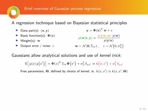
Brief overview of Gaussian process regression

A regression technique based on Bayesian statistical principlesI Data pair(s): (x,y)I Basis function(s): Φ(x)I Weight(s): wI Output error / noise: ε

y = Φ(x)T w + ε

p(w|x,y) =p(y|x,w) p(w)

p(y|x)

w ∼ N (0,Σw) , ε ∼ N(0, σ2

n

)

Gaussians allow analytical solutions and use of kernel trick:

E[y(x) y

(x′)]

= Φ(x)T ΣwΦ(x′)

+ σ2n δxx′ ≡ k

(x, x′

)+ σ2

n δxx′

Free parameters, Θ, defined by choice of kernel, ie. k(x, x′) ≡ k(x, x′,Θ)

Making predictions of y∗ given x∗:K(x,x) = k

(x = x, x′ = x

)y∗ = K(x∗,x)

[K(x,x) y + σ2

nI]

V[y∗] = K(x∗,x∗)−K(x∗,x)[K(x,x) + σ2

nI]−1

K(x,x∗)

4 / 13

Brief overview of Gaussian process regression

A regression technique based on Bayesian statistical principlesI Data pair(s): (x,y)I Basis function(s): Φ(x)I Weight(s): wI Output error / noise: ε

y = Φ(x)T w + ε

p(w|x,y) =p(y|x,w) p(w)

p(y|x)

w ∼ N (0,Σw) , ε ∼ N(0, σ2

n

)Gaussians allow analytical solutions and use of kernel trick:

E[y(x) y

(x′)]

= Φ(x)T ΣwΦ(x′)

+ σ2n δxx′ ≡ k

(x, x′

)+ σ2

n δxx′

Free parameters, Θ, defined by choice of kernel, ie. k(x, x′) ≡ k(x, x′,Θ)

Making predictions of y∗ given x∗:K(x,x) = k

(x = x, x′ = x

)y∗ = K(x∗,x)

[K(x,x) y + σ2

nI]

V[y∗] = K(x∗,x∗)−K(x∗,x)[K(x,x) + σ2

nI]−1

K(x,x∗)

4 / 13

Brief overview of Gaussian process regression

A regression technique based on Bayesian statistical principlesI Data pair(s): (x,y)I Basis function(s): Φ(x)I Weight(s): wI Output error / noise: ε

y = Φ(x)T w + ε

p(w|x,y) =p(y|x,w) p(w)

p(y|x)

w ∼ N (0,Σw) , ε ∼ N(0, σ2

n

)Gaussians allow analytical solutions and use of kernel trick:

E[y(x) y

(x′)]

= Φ(x)T ΣwΦ(x′)

+ σ2n δxx′ ≡ k

(x, x′

)+ σ2

n δxx′

Free parameters, Θ, defined by choice of kernel, ie. k(x, x′) ≡ k(x, x′,Θ)

Making predictions of y∗ given x∗:K(x,x) = k

(x = x, x′ = x

)y∗ = K(x∗,x)

[K(x,x) y + σ2

nI]

V[y∗] = K(x∗,x∗)−K(x∗,x)[K(x,x) + σ2

nI]−1

K(x,x∗)

4 / 13

Example: Squared-exponential (SE) kernel

Φ(x) = {φµ(x)}

φµ(x) = exp(−

(x− µ)2

2l2

) k(x, x′

)=√πlΣw exp

(−

(x− x′)2

2(√

2l)2

)Θ =

{σa =

√πlΣw, σl =

√2l}

Sample y drawnfrom model withrandom valuesfor w

More kernels are available, each with additional properties

For more info on statistical theory and constructing kernels, see:C. Bishop, Pattern Recognition and Machine Learning. New York, NY: Springer, 2006

C. Rasmussen and C. Williams, Gaussian Processes for Machine Learning. Cambridge, MA: MIT Press, 2006

5 / 13

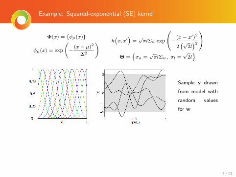
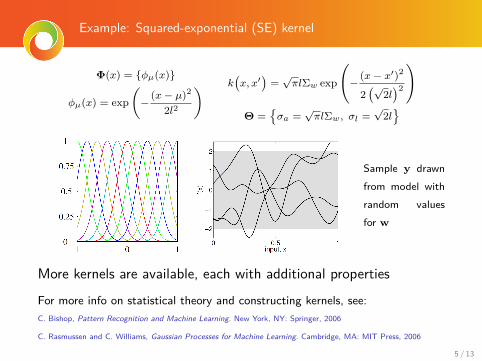
Example: Squared-exponential (SE) kernel

Φ(x) = {φµ(x)}

φµ(x) = exp(−

(x− µ)2

2l2

) k(x, x′

)=√πlΣw exp

(−

(x− x′)2

2(√

2l)2

)Θ =

{σa =

√πlΣw, σl =

√2l}

Sample y drawnfrom model withrandom valuesfor w

More kernels are available, each with additional properties

For more info on statistical theory and constructing kernels, see:C. Bishop, Pattern Recognition and Machine Learning. New York, NY: Springer, 2006

C. Rasmussen and C. Williams, Gaussian Processes for Machine Learning. Cambridge, MA: MIT Press, 2006

5 / 13

Optimizing the kernel hyperparameters using gradient-ascent

Denominator of Bayes’ Theorem is called the marginal likelihood:

p(y|x) =∫p(y|x,w) p(w) dw

Combined with Gaussian assumptions gives log-marginal-likelihood:

log p(y|x) = − 12 yT

(K + σ2

nI)−1 y− 1

2 log∣∣K + σ2

nI∣∣− 1

2nx log 2π

Goodness of fit Kernel complexity Size of data set

Cost function =⇒ maximized w.r.t the hyperparameters, Θ:I One of many ways to determine ΘI Gives Θ with maximum probability to match input dataI Gradient ascent search algorithm implemented with Monte

Carlo kernel restarts to ensure non-local maxima6 / 13

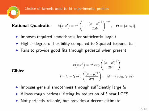
Choice of kernels used to fit experimental profiles

Rational Quadratic: k(x, x′

)= σ2

(1 +

(x− x′)2

2αl2

)−α, Θ = {σ, α, l}

I Imposes required smoothness for sufficiently large lI Higher degree of flexibility compared to Squared-ExponentialI Fails to provide good fits through pedestal when present

Gibbs:k(x, x′

)= σ2 exp

((x− x′)2

2l2

)l = l0 − l1 exp

((x− µ)2

2σ2l

), Θ = {σ, l0, l1, σl}

I Imposes general smoothness through sufficiently large l0I Allows rough pedestal fitting by reduction of l near LCFSI Not perfectly reliable, but provides a decent estimate

7 / 13

Decision chart of the extraction workflow

Extractdata from

DDAs

EFITdata

exists?

Reject

Calculatecoordinate

systems

ne,Tedata

exists?

PerformGP fits

Jump atρ > 0.8?

Gibbs Kernel

Regular Kernel

Ti exists?Perform GP

Ti = Te

nimpexists?

Perform GP

Use Zeff,est

Constr.q exists?

Use constrain

Apply bias

CalculateGK pa-

rameters

Applysanitychecks

Save

Y

N NY

Y

N

Y

N

Y

N

Y

N

8 / 13

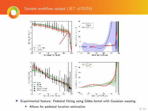
Sample workflow output (JET #70274)

I Experimental feature: Pedestal fitting using Gibbs kernel with Gaussian warpingI Allows for pedestal location estimation

9 / 13

Estimation of systematic coordinate mapping errors

Figure : JET #89091

Compared standard EFIT to EFITconstrained with Faraday rotation /MSE measurements

Figure : Normalized poloidal fluxdifferences with fitted 3rd-orderpolynomials for outer radii (red) andinner radii (blue)

10 / 13

Impact of estimated bias on profiles (JET #91366)

General result:

δρ ≈ 0.05 shift towards edge

For purposes of turbulence +transport integrated modelling,the primary concern is the shift ofthe boundary condition (pedestalshoulder location)

I Effect of this shift on suchmodelling has not yet beeninvestigated

11 / 13

Implemented checks to identify high quality data for validation

1. Integrated heat deposition profiles vs. injected heating powerI Validity check of heat deposition profiles

2. Heat deposition profiles vs. accumulated equipartition flux(Ti − Te)

I Validity check of fitted T profiles from GPI Equipartition flux does not yet account for isotope of main ion

(easily implementable)I For windows without CX, can be used to estimate how largeTi − Te can be

3. Integrated pressure (32nT ) profiles vs. total plasma energy

I Validity check of fitted n, T profiles from GP

Open to additional suggestions for checks, provided they arecomputationally quick to perform

12 / 13

Summary and next steps

Summary:I Gaussian process regression workflow for mass automated profile fitting (JET

data) for extracting parameter subspace for GK runsI Estimated bias between unconstrained and constrained EFIT (using Faraday

rotation and/or MSE) for boundary condition modification in integratedmodelling

I Basic sanity checks applied to identify high quality data set, used to testperformance of future NN within integrated modelling suites

Next Steps:I Improve checks to specify validation set for integrated modellingI Extend workflow to include data from other machines via adaptersI Detailed analysis of JET parameter space for problem characterization /

dimensionality reductionI Perform gyrokinetic simulations (QuaLiKiz, linear GENE) to build the training

set for NN

13 / 13

Using statistics on bias to estimate stochastic errors

In theory, x-errors can be applied by enhancing y-errors proportionally to gradient ofmodel fit without x-errors

K(x,x) + σ2nI =⇒ K(x,x) + σ2

nI + ∆yΣx∆Ty

I A. McHutchon and C. Rasmussen, “Gaussian process training with input noise,”Advances in Neural Information Processing Systems, pp. 1341–1349, 2011

I However, error bar size yields nonsensical fits −→ inappropriate error estimation14 / 13