Embed Size (px)
Citation preview
2004
8.29 Heat Exchanger Control and Optimization
B. G. LIPTÁK (1970, 1985, 1995, 2005)
INTRODUCTION
The transfer of heat is one of the most basic and best under-stood unit operations of the processing industries. Heat canbe transferred between the same phases (liquid to liquid, gasto gas), or phase change can occur on either the process side(in case of condensers, evaporators, and reboilers) or theutility side (in case of steam heater) of the heat exchanger.With the exception of evaporators, which are discussed inSection 8.23, the control and optimization of each of thesesystems will be discussed in this chapter.
The section is started with some general aspects, such asplantwide heat audits, heat exchanger safety, temperaturemeasurement advances, tuning, and heat-transfer dynamics.Next, it describes the basic components and controls of liquid-to-liquid heat exchangers, steam heaters, condensers, reboil-ers, and vaporizers. The section is concluded by the descrip-tion of more advanced control techniques, including override,cascade, feedforward, adaptive gain, model-based, and mul-tipurpose systems.
GENERAL CONSIDERATIONS
In a processing plant, the heat exchanger as a unit operationis part of larger plantwide unit operations, serving the heatingor cooling needs of all the processes in the plant. By the useof BTU flowmeters (Section 2.3 in Chapter 2 in the firstvolume of this handbook), one can obtain a plantwide energyaudit (Figure 8.29a) and provide historical plots of both thetotal amounts of energy used and of the efficiency at whichit was used. If the individual heat exchanger controls of theplant are optimized, such plantwide information can be usefulin such decisions as when to clean heat-transfer surfaces orwhat the optimum cooling water temperature or steam supplypressure and superheat values are.
Temperature Detection and Transmission
Chapter 4 of the first volume of this handbook is devoted tothe description of the capabilities of the various temperaturedetectors available. The vast majority of temperature mea-surements are made with either a thermocouple (TC) or aresistance temperature detector (RTD). Higher purity mate-
rials and improved manufacturing processes have providedsensors that more closely match theoretical curves and exhibitlower drift than sensors of the 1980s and the 1990s.
More advanced transmitters incorporate the ability tomatch the sensor to the transmitter to minimize this error.Typical accuracies are about ±0.4°F. For higher precision, atleast one vendor offers a bath calibration technique thatallows the transmitter to capture actual values output by theRTD or thermocouple at specific temperatures. This methodprovides system accuracies of about ±0.02°F (0.1°C) forRTDs and about ±2°F (1°C) for thermocouple measurements.
The array of intelligent temperature transmitters on themarket seems almost endless. Some common features of theleading models are universal inputs from any TC, RTD, mV,resistance, or potentiometer; loop-powered with 0–20/4–20 mA output; digital outputs; and configuration with push-buttons, PC software, or a handheld configurator. Choices mustbe made concerning the protocol required: HART, Founda-tion Fieldbus, Profibus, vendor proprietary, Ethernet, or just
FIG. 8.29aA plantwide energy audit can determine the useful portion of theenergy that is represented by fuel consumed at the boiler(s) andby electric energy used by the chiller(s) that actually reaches theprocess.
3
1
4
5
6
7
8
HeatloadsFeed
water
Boiler
Chiller
M
Fuel
Steam2
12 14 16
888Cooling
loads
Chwr
ChwsElectricpower
11
10
© 2006 by Béla Lipták
8.29 Heat Exchanger Control and Optimization 2005
4–20 mA. Some field locations will benefit from local indica-tion, and this feature is optional with most manufacturers.
Direct connection of temperature sensors to input sub-systems of DCSs or PLCs is an alternative to using a tem-perature transmitter for each measurement. This may soundlike a way to cut costs. In actuality, on an installed basis, itis more expensive, far less accurate, and not as robust. Thebenefits of using transmitters include higher precision, sensor-transmitter systems calibrated to the range of interest, betterRFI immunity and noise rejection, transmitter diagnostics,lower wiring costs, less expensive I/O cards, faster loopchecks, and shorter start-ups.
Process Characteristics
Heat transfer is one of the best understood processes, and assuch, it has good potentials for modeling and optimization.Before discussing the control of heat exchangers, the degreesof freedom, scaling, dynamics, and tuning of this unit oper-ation will be briefly discussed.
Degrees of Freedom Chapter 2’s Section 2.1, in connec-tion with Figures 2.1r and 2.1s, provides a detailed discussionof the determination of the degrees of freedom of any process.The degrees of freedom of a process define the maximumnumber of independently acting automatic controllers thatcan be placed on a process.
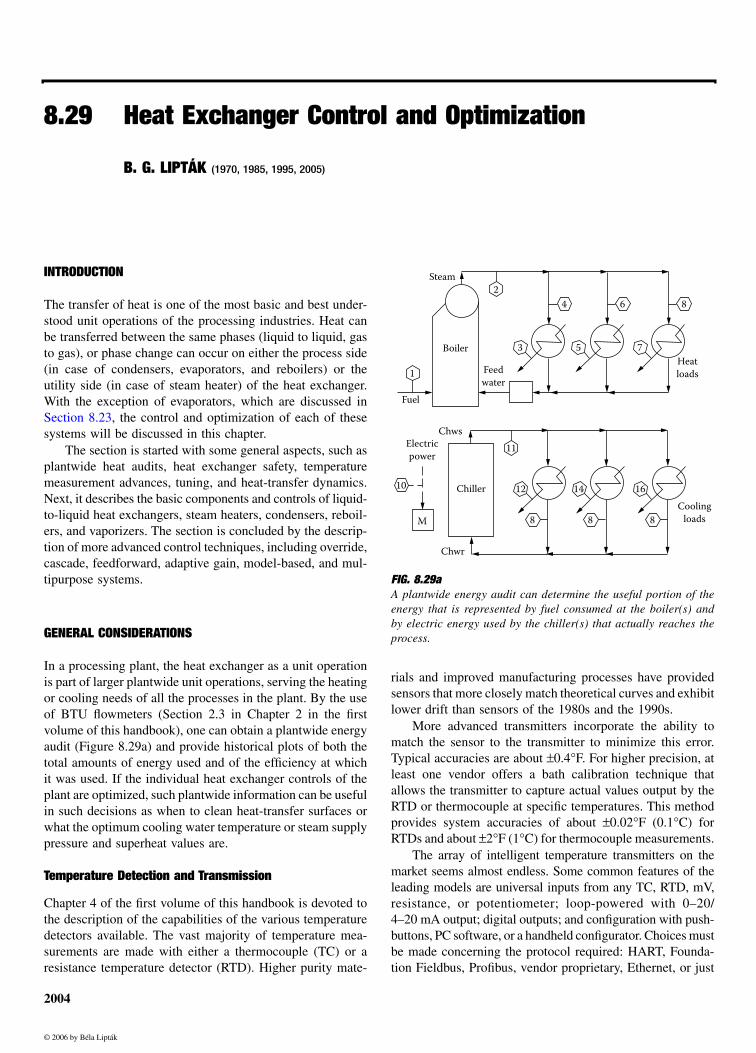
Figure 8.29b shows a steam heater with its variables anddefining parameters. The temperatures and flows are vari-ables, and the specific and latent heats are parameters. Theavailable degrees of freedom are determined by subtractingthe number of system-defining equations from the numberof process variables:
8.29(1)
In this case, there are four process variables and onedefining equation, which is that of the conservation of energy,based on the first law of thermodynamics:
8.29(2)
Therefore, this system has three degrees of freedom; thus,a maximum of three automatic controllers can be placed on it.
In a liquid-to-liquid heat exchanger, there are four tem-perature and two flow variables with still only one (conser-vation of energy) defining equation, resulting in five degreesof freedom:
8.29(3)
In a steam-heated reboiler or in a condenser cooled by avaporizing refrigerant (assuming no superheating or super-cooling), there are only two flow variables and one definingequation:
8.29(4)
In these cases there is only a single degree of freedom,and therefore on these processes only one automatic control-ler can be used.
In the majority of installations, fewer controllers are usedthan the available degrees of freedom, but every once in awhile mistakes are made by using too many controllers andthereby overdefining the process.
Scaling, Gain, and Time Constant Scaling is the conversionfrom engineering units to fractions or percentages. For thescaling of a heat-transfer equation, a detailed example hasbeen provided in connection with Figure 8.5r.
The steady-state gain of a heat-transfer process is theratio of the percentage change in controlled temperature thatresult from a 1% change in the flow through the control valvethat controls that temperature.
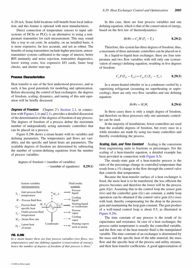
Because the heat-transfer surface of a heat exchanger isfixed, the more heat is to be transferred, the less efficient theprocess becomes and therefore the lower will be the processgain (Gp). Assuming that in the control loop the sensor gain(Gs) and the controller gain (Gc) are constant, a stable loopoperation can be obtained if the control valve gain (Gv) riseswith load, thereby compensating for the drop in the processgain and maintaining the loop gain constant. The gain productof a well-tuned control loop is about 0.5, as illustrated inFigure 8.29c.
The time constant of any process is the result of itscapacitance and resistance. In case of a heat exchanger, theprocess outlet temperature is usually the controlled variable,and the flow rate of the heat-transfer fluid is the manipulatedvariable. The time constant of an exchanger is determined bythe mass and the specific heat of the tube material, the massflow and the specific heat of the process and utility streams,and their heat-transfer coefficients. A good approximation of
FIG. 8.29bIn a steam heater there are four process variables (two flows, twotemperatures) and one defining equation (conservation of energy),hence the number of degrees of freedom of that process is three.1
degrees of freedom number of variablesnumb
=−( )
( eer of equations)
ProcessliquidCoolingliquidHeating liquidor condensateProcessvaporCoolingvaporHeating vaporssuch as steam
Fluid mediasymbols:
Condensate
Ws, l
W, T1 Cp,T2
System variablesand parameters:
Inlet process fluidtemperatureT1 –
W – Process fluid flow
Cp –Process fluidspecific heat
T2 –Outlet process fluidtemperature
Ws – Steam flow rate
Hs =Latent heatof steam
HsWs C W T Tp= −( )2 1
C F T T C F T Tp h h pc c c c( ) ( )1 2 2 1− = −
HsWs H W= 1 1
© 2006 by Béla Lipták
2006 Control and Optimization of Unit Operations
a heat exchanger’s time constant can be obtained with theempirical formula:
8.29(5)
whereτ = the time constant in secondsK = 100 for English units, and 200 for SI units
mT = the total mass of the tubes in lb (kg)CpT = the specific heat of the tube material in BTU/lbm
(kJ/kgK)Fw = the flow rate of the warm stream in lb/sec (kg/sec)Cpw = the specific heat of the warm fluid in BTU/lbm
(kJ/kgK)Fc = the flow rate of the cold stream in lb/sec (kg/sec)Cpc = the specific heat of the cold fluid in BTU/lbm (kJ/kgK)
In process industry heat exchangers, the time constantsare usually between 5 sec and 2 min.
Dead Time and Tuning Before the new flow rate or temper-ature of the heat-transfer fluid can start to have an impact onthe heat balance, first it has to get to the heat-transfer surface
of the exchanger. Therefore, dead time is also called trans-portation lag, because it is the time it takes for the heat-transfer fluid to transport (displace) the contents of theexchanger and its associated piping.
The dead time is the worst enemy of control, becauseuntil it has expired, a change in the heat-transfer fluid flow(or temperature) will not even start to have an observableeffect on the process. For a heat exchanger, the dead time isusually between 1 and 30 sec. When the equipment is cor-rectly designed, the dead time is much less than the timeconstant.
Tuning is discussed in detail in Sections 2.35 to 2.38 inChapter 2 in this volume. The controller gain is adjusted sothat the loop gain (the gain product of the loop components)will be around 0.5. In case of variable gain processes, suchas heat transfer, one usually tries to compensate for the gainvariations of the process by using a control valve character-istic that compensates for it. In case of the more criticalprocesses, adaptive (Section 2.19) and model-based (Sections2.13 to 2.18 in Chapter 2) controls can be used.
Control loops can be tuned by considering the dynamicsof only the process (open-loop method) or evaluating theresponse of the complete loop (closed-loop method). Becausethe period of oscillation of all control loops (P) is somemultiple (around 3.5 to 4.0) of their dead time, the integraland derivative settings of PID controllers are generallyadjusted as a function of the dead time of the process.
For noninteracting control loops with zero dead time, theintegral setting (minutes/repeat) is about 50% and the deriv-ative is about 18% of the period of oscillation. As dead timerises, these percentages drop. If the dead time reaches 50%of the time constant, I = 40%, D = 16%, and if dead timeequals the time constant, I = 33% and D = 13% of the periodof oscillation. For a comparison of the various tuning criteria,refer to Table 2.35l, and for the load and set point responsesof the various tuning methods, see Figures 2.35o, p, and qin Chapter 2.
As will be shown later, when tuning the feedforwardportion of a control loop, one has to separately consider thesteady-state portion of the heat-transfer process (flow timestemperature difference) and its dynamic compensation. Thedynamic compensation of the steady-state model by alead/lag element is necessary, because the response is notinstantaneous, but affected by both the dead time and thetime constant of the process.
Safety
Heat exchangers are a class of process equipment requiringspecial relief considerations, because of the potential needfor protection against thermal expansion, external fire,blocked outlet, and tube rupture cases.
Blocked-In Exchangers Heat exchangers frequently havevalves located on both their inlet and outlet piping. When
FIG. 8.29cIf the process gain varies with load, such as is the case of heat-transfer processes, the gain product of the loop can be held constantby using a valve whose gain variation with load will compensatefor the process gain variation.
Load
Load
For stableControl:Gc ⋅ Gv ⋅ Gp ⋅ Gs = 0.5
Load
Load(u)
Load
Setpoint(r)
Cont
rolle
rga
in(G
c)
Processgain(G
p)
Sensorgain(Gs)
Valve gain(Gv)
Gv
Gc
Gs
e
bc
Gp
m1m
−+
++
τ =•
• • •K
m C
F C F CT pT
w pw c pc
© 2006 by Béla Lipták
8.29 Heat Exchanger Control and Optimization 2007
these valves are all closed, the exchanger is “blocked in.” Ifthe cold side of the heat exchanger can be blocked in, reliefdevices are installed to provide protection against thermalexpansion of liquids in the exchanger. This is always donefor the cold side of an exchanger where the liquid can beheated by the hot fluid on the other side, or can be heated byambient temperature, while sitting with the inlet and outletvalves closed.
No relief device is necessary for the protection of eitherside of an exchanger that cannot be blocked in. In suchinstallations it is assumed that the relief of the unit is takencare of by the relief device on the related tank or equipment.
Liquid Refrigerants When liquid refrigerants are used, arelief device should always be provided for the protection ofthe refrigerant side, if the refrigerant side can be blocked inand if the vapor pressure of the refrigerant can exceed thedesign pressure of the exchanger, when its temperature risesto that of the hot side.
A relief device should also be provided whenever thevapor pressure of the material flowing at 100°F (37.8°C) isgreater than the design pressure of the exchanger. This rec-ommendation is somewhat site-specific and is based on anassumed (maximum) ambient temperature of 100°F(37.8°C). This temperature should be modified according tothe geographical areas involved.
Gas-Fired Tubular Heaters Direct gas-fired tubular heatersare always protected by relief valves on their tube side. Thevalve is normally sized for the design heat-transfer rating ofthe heater and must initially handle a fluid rate correspondingto the rate of thermal expansion in the tubes when they areblocked in.
When designing fired heaters, there should be no blockvalve on its outlet. This is because PRVs for high-temperatureservices exceeding 550°F are not available with dependableseat and seal materials.
Tube Rupture Consideration should be given to relief pro-tection of low-pressure equipment in the event an exchangertube should rupture because of corrosion or vibration or dueto thermal shock. ASME Code, Section VIII, Division 1,Paragraph UG-133(d) requires such protection.
This consideration is particularly critical when the low-pressure side design pressure is less than the operating pres-sure on the high-pressure side. In terms of high- and low-pressure side design pressures, PRV protection against tuberupture is recommended, if the design pressure of the low-pressure side is less than 77% of the high-pressure side.
For advice on the sizing of PRVs to protect against over-pressure caused by tube rupture, refer to Section 7.15 inChapter 7 in the first volume of this handbook. The PRVthat is to protect the exchanger should be located eitherdirectly on the exchanger, or very close to it.
BASIC CONTROLS
In the following paragraphs, the basic controls of liquid-liquidheat exchangers, steam heaters, condensers, vaporizers, andreboilers will be discussed. This will be followed by a descrip-tion of more advanced controls for these unit operations.
Liquid-Liquid Heat Exchanger Controls
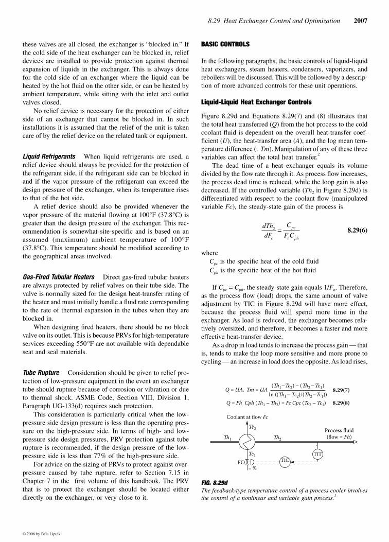
Figure 8.29d and Equations 8.29(7) and (8) illustrates thatthe total heat transferred (Q) from the hot process to the coldcoolant fluid is dependent on the overall heat-transfer coef-ficient (U), the heat-transfer area (A), and the log mean tem-perature difference (. Tm). Manipulation of any of these threevariables can affect the total heat transfer.2
The dead time of a heat exchanger equals its volumedivided by the flow rate through it. As process flow increases,the process dead time is reduced, while the loop gain is alsodecreased. If the controlled variable (Th2 in Figure 8.29d) isdifferentiated with respect to the coolant flow (manipulatedvariable Fc), the steady-state gain of the process is
8.29(6)
whereCpc is the specific heat of the cold fluid Cph is the specific heat of the hot fluid
If Cpc = Cph, the steady-state gain equals 1/Fn. Therefore,as the process flow (load) drops, the same amount of valveadjustment by TIC in Figure 8.29d will have more effect,because the process fluid will spend more time in theexchanger. As load is reduced, the exchanger becomes rela-tively oversized, and therefore, it becomes a faster and moreeffective heat-transfer device.
As a drop in load tends to increase the process gain — thatis, tends to make the loop more sensitive and more prone tocycling — an increase in load does the opposite. As load rises,
FIG. 8.29d The feedback-type temperature control of a process cooler involvesthe control of a nonlinear and variable gain process.1
dTh
dF
C
F Cc
pc
h ph
2 =
Process fluid(flow = Fh)
Coolant at flow Fc
Tc2
�1 �2
Tc1
FO= %
(�1−Tc2) − (�2 − Tc1)In ((�1 − Tc2)/(�2−Tc1))
Q = UA. Tm = UA
Q = Fh Cph (�1 − �2) = Fc Cpc (Tc2 − Tc1)
TICTIT
8.29(7)
8.29(8)
⋅
© 2006 by Béla Lipták
2008 Control and Optimization of Unit Operations
the exchanger becomes less and less effective, more and moreundersized; therefore, it takes more time for the TIC to makea correction. An increase in load thus will make the loopsluggish, as the residence and dead times are reduced andthe process gain is lowered.
As the process gain of all heat exchangers varies withload, it would not be possible to tune the TIC in Figure 8.29dfor more than one load, if all other loop gains remainedconstant, while the process gain varied. In order to minimizecycling, the TIC is usually tuned for the minimum load (max-imum process gain). Therefore, if not automatically compen-sated, it can act sluggish at higher loads.
As the process gain drops with rising load, the total loopgain can be held relatively constant by introducing a loopcomponent whose gain rises with load. Such an element isan equal-percentage valve, which can compensate for thevariable gain process. This is a good solution if the temper-ature difference through the exchanger (Th1 − Th2) is con-stant.3 If it is not constant, feedforward compensation of thegain is required, as will be discussed later.
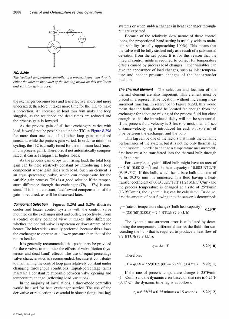
Component Selection Figures 8.29d and 8.29e illustratecooler and heater control systems with the control valvemounted on the exchanger inlet and outlet, respectively. Froma control quality point of view, it makes little differencewhether the control valve is upstream or downstream of theheater. The inlet side is usually preferred, because this allowsthe exchanger to operate at a lower pressure than that of thereturn header.
It is generally recommended that positioners be providedfor these valves to minimize the effects of valve friction (hys-teresis and dead band) effects. The use of equal-percentagevalve characteristics is recommended, because it contributesto maintaining the control loop gain relatively constant underchanging throughput conditions. Equal-percentage trimsmaintain a constant relationship between valve opening andtemperature change (reflecting load variations).
In the majority of installations, a three-mode controllerwould be used for heat exchanger service. The use of thederivative or rate action is essential in slower (long time-lag)
systems or when sudden changes in heat exchanger through-put are expected.
Because of the relatively slow nature of these controlloops, the proportional band setting is usually wide to main-tain stability (usually approaching 100%). This means thatthe valve will be fully stroked only as a result of a substantialdeviation from the set point. It is for this reason that theintegral control mode is required to correct for temperatureoffsets caused by process load changes. Other variables cangive the appearance of load changes, such as inlet tempera-ture and header pressure changes of the heat-transfermedium.
The Thermal Element The selection and location of thethermal element are also important. This element must beplaced in a representative location, without increasing mea-surement time lag. In reference to Figure 8.29d, this wouldmean that the bulb should be located far enough from theexchanger for adequate mixing of the process fluid but closeenough so that the introduced delay will not be substantial.If the process fluid velocity is 3 ft/s (0.9 m/s), then a 1 secdistance-velocity lag is introduced for each 3 ft (0.9 m) ofpipe between the exchanger and the bulb.
This lag can be one of the factors that limits the dynamicperformance of the system, but it is not the only thermal lagin the system. In order to change a temperature measurement,first heat must be transferred into the thermal bulb throughits fixed area.
For example, a typical filled bulb might have an area of0.02 ft2 (0.0018 m2) and the heat capacity of 0.005 BTU/°F(9.49 J/°C). If this bulb, which has a bare-bulb diameter of3/8 in. (9.375 mm), is immersed in a fluid having a heat-transfer coefficient of 60 BTU/h/°F/ft2 (1.23 MJ/h/°C/m2) andthe process temperature is changed at a rate of 25°F/min(13.9°C/min), the dynamic lag can be calculated. To do so,first the amount of heat flowing into the sensor is determined:
8.29(9)
The dynamic measurement error is calculated by deter-mining the temperature differential across the fluid film sur-rounding the bulb that is required to produce a heat flow of7.2 BTU/h (7.9 kJ/h):
8.29(10)
Therefore,
8.29(11)
If the rate of process temperature change is 25°F/min(14°C/min) and the dynamic error based on that rate is 6.25°F(3.47°C), the dynamic time lag is as follows:
8.29(12)
FIG. 8.29e The feedback temperature controller of a process heater can throttleeither the inlet or the outlet of the heating media on this nonlinearand variable gain process.1
TICFC
TIT
×
q = ( ) (rate of temperature change bulb heat capacityy
BTU h kJ/h
)
( )( )( . ) . / ( . )= =25 60 0 005 7 5 7 9
q Ah T= .
. T q Ah= = = ° °/ . /( . )( ) . ( . )7 5 0 02 60 6 25 3 47F C
to = = =6 25 25 0 25 15. / . minutes seconds
© 2006 by Béla Lipták
8.29 Heat Exchanger Control and Optimization 2009
This lag can also be calculated as
8.29(13)
Bulb time lags vary from a few seconds to minutes,depending on their mass, heat-transfer area, and the processfluid being detected. Measurement of gas temperatures at lowvelocity involves the longest time lags, and measuring water(or dilute solutions) at high velocity results in the shortestlags.
The addition to the sensor lag of a thermowell will furtherincrease the total lag time, but in most industrial installations,thermowells are necessary for reasons of safety and mainte-nance. When they are used, it is important to eliminate anyair gaps between the bulb and the socket.
One method of reducing time lag is by miniaturizing thesensing element. Conventional thermometers are not suitablefor all temperature measurement applications. For example,the accurate detection of high-temperature gases (500 to2000°C) at low velocities (3 to 5 ft/s) is a problem, even forthermocouples. This is because conductance through the leadwires and radiation both tend to alter the sensor temperaturefaster than the low velocity gas flow can resupply the lost heat.In such applications (fuel cell controls are prime examples),optical fiber thermometry is a good choice.
Thermocouples are usually not accurate enough for theprecise measurement of temperature differences and are notfast enough to detect high-speed variations in temperature.RTDs can detect temperature differences of 10°F at a mea-surement error of ±0.04°F. If high-speed response is desired,thermistors or infrared detectors should be considered.
In the conventional control loop, the measurement lag isonly part of the total time lag of the control loop. For exam-ple, an air heater might have a total lag of 15 min. Of thislag, 14 min represent the process lag, 50 sec the bulb lag,and 10 sec is the control valve’s contribution to the total timelag.
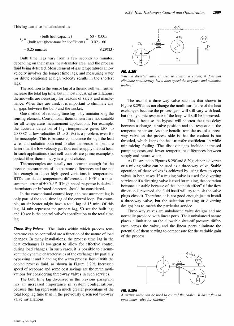
Three-Way Valves The limits within which process tem-perature can be controlled are a function of the nature of loadchanges. In many installations, the process time lag in theheat exchanger is too great to allow for effective controlduring load changes. In such cases, it is possible to circum-vent the dynamic characteristics of the exchanger by partiallybypassing it and blending the warm process liquid with thecooled process fluid, as shown in Figure 8.29f. Increasedspeed of response and some cost savings are the main moti-vations for considering three-way valves in such services.
The bulb time lag discussed in the previous paragraphhas an increased importance in system configurations,because this lag represents a much greater percentage of thetotal loop lag time than in the previously discussed two-wayvalve installations.
The use of a three-way valve such as that shown inFigure 8.29f does not change the nonlinear nature of the heatexchanger, because the process gain will still vary with load,but the dynamic response of the loop will still be improved.
This is because the bypass will shorten the time delaybetween a change in valve position and the response at thetemperature sensor. Another benefit from the use of a three-way valve on the process side is that the coolant is notthrottled, which keeps the heat-transfer coefficient up whileminimizing fouling. The disadvantages include increasedpumping costs and lower temperature differences betweensupply and return water.
As illustrated in Figures 8.29f and 8.29g, either a diverteror a mixing valve can be used as a three-way valve. Stableoperation of these valves is achieved by using flow to openvalves in both cases. If a mixing valve is used for divertingservice or if a diverting valve is used for mixing, the operationbecomes unstable because of the “bathtub effect” (if the flowdirection is reversed, the fluid itself will try to push the valveplugs closed). Therefore, it is not good enough just to installa three-way valve, but the selection (mixing or divertingdesign) has to match the particular service.
Three-way valves are unbalanced valve designs and arenormally provided with linear ports. Their unbalanced natureplaces a limitation on the allowable shut-off pressure differ-ence across the valve, and the linear ports eliminate thepotential of them serving to compensate for the variable gainof the process.
to = ( )( )(
bulb heat capacitybulb area heat-transfeer coefficient)
..
= ⋅⋅
60 0 0050 02 60
= 0 25. minutes
FIG. 8.29f When a diverter valve is used to control a cooler, it does noteliminate nonlinearity, but it does speed the response and minimizefouling.1
FIG. 8.29gA mixing valve can be used to control the cooler. It has a flow toopen inner valve for stability.1
FO
Tc1
�1
Tc2
�2
TIT
TIC
⋅
TIC
TITFO
© 2006 by Béla Lipták
2010 Control and Optimization of Unit Operations
Misalignment or distortion in a three-way control valveinstallation can cause binding, leakage at the seats, dead band,and packing friction. Such conditions commonly arise whenthree-way valves are used in high-temperature applications.This is because, having been installed at ambient conditionsand rigidly connected at three flanges, the valve cannotaccommodate pipeline expansion caused by high process tem-peratures, and therefore distortion results.
Similarly, in mixing applications, when the temperaturedifference between the two ports is substantial, the resultingdifferential expansion can also cause distortion. For thesereasons, the use of three-way valves at temperatures above500°F (260°C) or at differential temperatures exceeding300°F (167°C) is not recommended.
The choice of three-way valve location is normally basedon pressure and temperature considerations, with theupstream location (Figure 8.29f) usually being favored forreasons of uniformity of valve temperature. When the over-riding consideration is the desire to operate the exchanger ata high pressure, the downstream location might be selected.
Cooling Water Conservation Figure 8.29h modifies the con-trol systems shown earlier by adding a controller to serve cool-ing water conservation. The TIC-01 in Figure 8.29h is set ata relatively high value to maximize the outlet cooling watertemperature, thereby minimizing the rate of cooling waterusage.
When using this approach, one should be careful to makesure that the cooling water contains chemicals to prevent tubefouling under higher return water temperature conditions. Ifthe cooling water supply is sufficient and the TIC-01 set pointis properly selected, this system on the one hand will con-serve water and, on the other, will also protect against exces-sively high outlet water temperature.
Unfortunately, this configuration will not yield stablecontrol, because controlling temperature through manipula-
tion of its own flow results in a limit cycle. The cause of thisinstability is that the output of TIC-01 affects the dead timeof the process that it controls. This comes about because ifTIC-01 detects a temperature rise, it opens its valve, causinga sudden drop in temperature as the process dead time is alsoreduced.
As TIC-01 senses this sudden drop in temperature, it willclose its valve, but because this also increases the processdead time, the resulting temperature will rise slowly.4 Thislimit cycle, consisting of segments of slow rise and fast fall,will also affect the performance of TIC-02 through interactionbetween the loops. The amplitude of the cycle can be reducedby increasing the proportional band (reducing the gain) ofTIC-01, which will also increase the period of oscillation.4
The only way to eliminate this oscillation altogether isto fix the process dead time. This can be done by the additionof a recirculating pump, which will return part of the heatedwater back to the inlet. As can be seen, there is no easy wayto make this configuration stable, and for that reason, the bestsolution is to avoid its use.
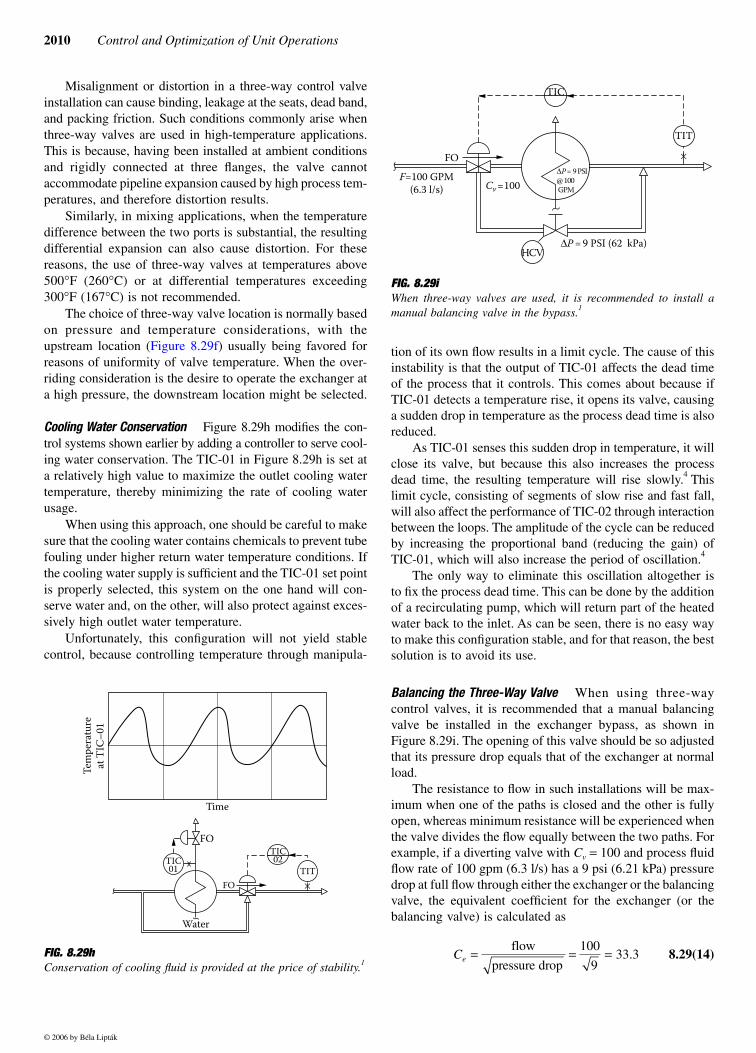
Balancing the Three-Way Valve When using three-waycontrol valves, it is recommended that a manual balancingvalve be installed in the exchanger bypass, as shown inFigure 8.29i. The opening of this valve should be so adjustedthat its pressure drop equals that of the exchanger at normalload.
The resistance to flow in such installations will be max-imum when one of the paths is closed and the other is fullyopen, whereas minimum resistance will be experienced whenthe valve divides the flow equally between the two paths. Forexample, if a diverting valve with Cv = 100 and process fluidflow rate of 100 gpm (6.3 l/s) has a 9 psi (6.21 kPa) pressuredrop at full flow through either the exchanger or the balancingvalve, the equivalent coefficient for the exchanger (or thebalancing valve) is calculated as
8.29(14)FIG. 8.29h Conservation of cooling fluid is provided at the price of stability.1
Time
Tem
pera
ture
at T
IC–0
1
TIC02TIC
01 TITFO
Water
FO
TIC01
×
FIG. 8.29i When three-way valves are used, it is recommended to install amanual balancing valve in the bypass.1
TIC
HCV
TIT
FO∆P= 9 PSI@ 100 GPM
∆P = 9 PSI (62 kPa)
F=100 GPM(6.3 l/s) Cv =100
×
Ce = = =flow
pressure drop
100
933 3.
© 2006 by Béla Lipták
8.29 Heat Exchanger Control and Optimization 2011
Therefore, in either extreme position (closed or fullbypass), the total system resistance expressed in valve coef-ficient units is
8.29(15)
When the valve divides the flow equally between the twopaths, because of the linear characteristics of three-wayvalves, its coefficient at each port will be Cv = 50. Theequivalent coefficient (Ce = 33.3) of the exchanger and bal-ancing valve being unaffected, the total system resistance invalve coefficient units is 2Ct:
8.29(16)
If the total pressure drop through the system is calculatedwhen the valve is in its extreme and when it is in its middleposition, handling the same 100 gpm (6.3 l/s) flow, the fol-lowing pressure drops are found:
8.29(17)
8.29(18)
These results indicate that the system drop in one of theextreme positions is more than three times that of the pressuredrop in the middle position.
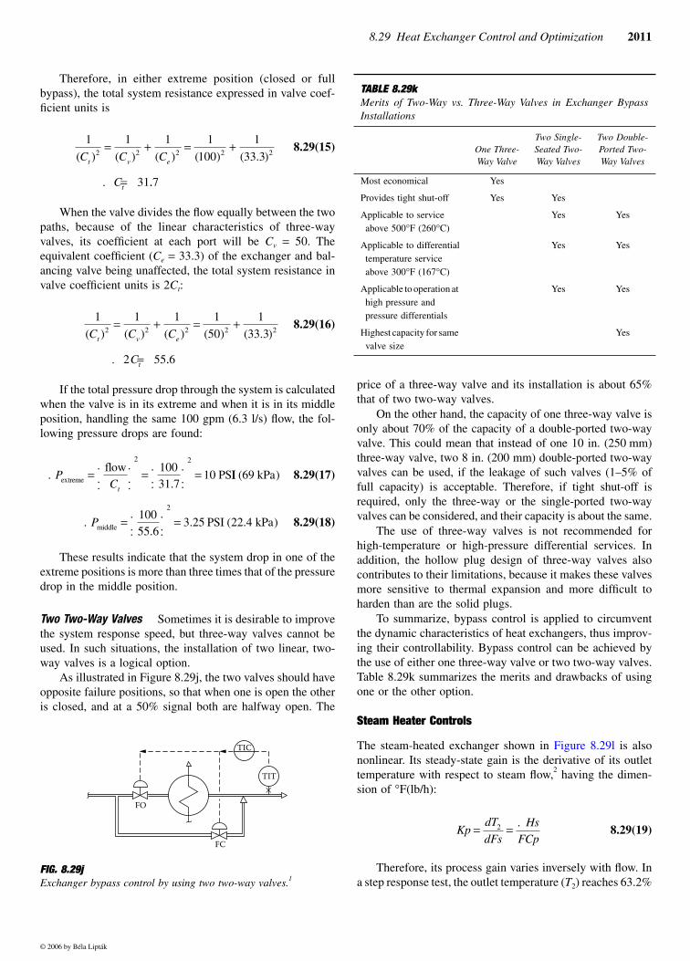
Two Two-Way Valves Sometimes it is desirable to improvethe system response speed, but three-way valves cannot beused. In such situations, the installation of two linear, two-way valves is a logical option.
As illustrated in Figure 8.29j, the two valves should haveopposite failure positions, so that when one is open the otheris closed, and at a 50% signal both are halfway open. The
price of a three-way valve and its installation is about 65%that of two two-way valves.
On the other hand, the capacity of one three-way valve isonly about 70% of the capacity of a double-ported two-wayvalve. This could mean that instead of one 10 in. (250 mm)three-way valve, two 8 in. (200 mm) double-ported two-wayvalves can be used, if the leakage of such valves (1–5% offull capacity) is acceptable. Therefore, if tight shut-off isrequired, only the three-way or the single-ported two-wayvalves can be considered, and their capacity is about the same.
The use of three-way valves is not recommended forhigh-temperature or high-pressure differential services. Inaddition, the hollow plug design of three-way valves alsocontributes to their limitations, because it makes these valvesmore sensitive to thermal expansion and more difficult toharden than are the solid plugs.
To summarize, bypass control is applied to circumventthe dynamic characteristics of heat exchangers, thus improv-ing their controllability. Bypass control can be achieved bythe use of either one three-way valve or two two-way valves.Table 8.29k summarizes the merits and drawbacks of usingone or the other option.
Steam Heater Controls
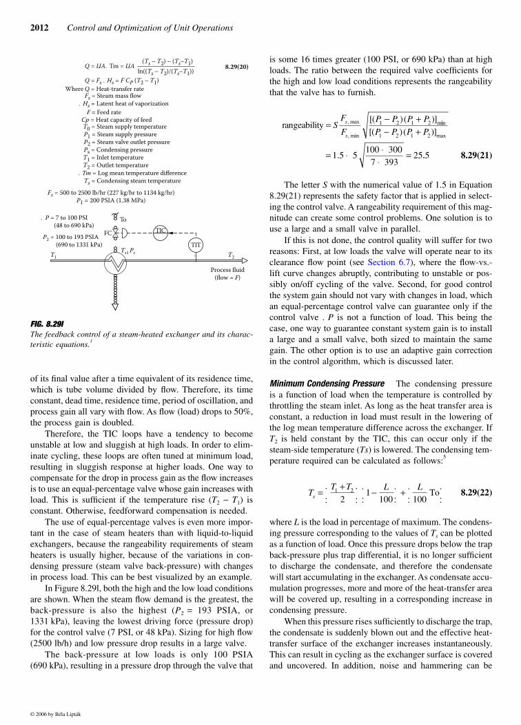
The steam-heated exchanger shown in Figure 8.29l is alsononlinear. Its steady-state gain is the derivative of its outlettemperature with respect to steam flow,2 having the dimen-sion of °F(lb/h):
8.29(19)
Therefore, its process gain varies inversely with flow. Ina step response test, the outlet temperature (T2) reaches 63.2%
FIG. 8.29jExchanger bypass control by using two two-way valves.1
1 1 1 1
100
1
33 3
31
2 2 2 2 2( ) ( ) ( ) ( ) ( . )C C C
C
t v e
t
= + = +
. = ..7
1 1 1 1
50
1
33 3
2 55
2 2 2 2 2( ) ( ) ( ) ( ) ( . )C C C
C
t v e
t
= + = +
. = ..6
. PCt
extreme
flowPS=
.
...
..=
.
.....
=2 2
10031 7
10.
II kPa( )69
. Pmiddle PSI kPa=...
.
..=100
55 63 25 22 4
2
.. ( . )
TIC
TIT
FO
FC
×
TABLE 8.29kMerits of Two-Way vs. Three-Way Valves in Exchanger BypassInstallations
One Three-Way Valve
Two Single-Seated Two-Way Valves
Two Double-Ported Two-Way Valves
Most economical Yes
Provides tight shut-off Yes Yes
Applicable to service above 500°F (260°C)
Yes Yes
Applicable to differentialtemperature serviceabove 300°F (167°C)
Yes Yes
Applicable to operation at high pressure and pressure differentials
Yes Yes
Highest capacity for same valve size
Yes
KpdT
dFsHs
FCp= =2 .
© 2006 by Béla Lipták
2012 Control and Optimization of Unit Operations
of its final value after a time equivalent of its residence time,which is tube volume divided by flow. Therefore, its timeconstant, dead time, residence time, period of oscillation, andprocess gain all vary with flow. As flow (load) drops to 50%,the process gain is doubled.
Therefore, the TIC loops have a tendency to becomeunstable at low and sluggish at high loads. In order to elim-inate cycling, these loops are often tuned at minimum load,resulting in sluggish response at higher loads. One way tocompensate for the drop in process gain as the flow increasesis to use an equal-percentage valve whose gain increases withload. This is sufficient if the temperature rise (T2 − T1) isconstant. Otherwise, feedforward compensation is needed.
The use of equal-percentage valves is even more impor-tant in the case of steam heaters than with liquid-to-liquidexchangers, because the rangeability requirements of steamheaters is usually higher, because of the variations in con-densing pressure (steam valve back-pressure) with changesin process load. This can be best visualized by an example.
In Figure 8.29l, both the high and the low load conditionsare shown. When the steam flow demand is the greatest, theback-pressure is also the highest (P2 = 193 PSIA, or1331 kPa), leaving the lowest driving force (pressure drop)for the control valve (7 PSI, or 48 kPa). Sizing for high flow(2500 lb/h) and low pressure drop results in a large valve.
The back-pressure at low loads is only 100 PSIA(690 kPa), resulting in a pressure drop through the valve that
is some 16 times greater (100 PSI, or 690 kPa) than at highloads. The ratio between the required valve coefficients forthe high and low load conditions represents the rangeabilitythat the valve has to furnish.
8.29(21)
The letter S with the numerical value of 1.5 in Equation8.29(21) represents the safety factor that is applied in select-ing the control valve. A rangeability requirement of this mag-nitude can create some control problems. One solution is touse a large and a small valve in parallel.
If this is not done, the control quality will suffer for tworeasons: First, at low loads the valve will operate near to itsclearance flow point (see Section 6.7), where the flow-vs.-lift curve changes abruptly, contributing to unstable or pos-sibly on/off cycling of the valve. Second, for good controlthe system gain should not vary with changes in load, whichan equal-percentage control valve can guarantee only if thecontrol valve . P is not a function of load. This being thecase, one way to guarantee constant system gain is to installa large and a small valve, both sized to maintain the samegain. The other option is to use an adaptive gain correctionin the control algorithm, which is discussed later.
Minimum Condensing Pressure The condensing pressureis a function of load when the temperature is controlled bythrottling the steam inlet. As long as the heat transfer area isconstant, a reduction in load must result in the lowering ofthe log mean temperature difference across the exchanger. IfT2 is held constant by the TIC, this can occur only if thesteam-side temperature (Ts) is lowered. The condensing tem-perature required can be calculated as follows:5
8.29(22)
where L is the load in percentage of maximum. The condens-ing pressure corresponding to the values of Ts can be plottedas a function of load. Once this pressure drops below the trapback-pressure plus trap differential, it is no longer sufficientto discharge the condensate, and therefore the condensatewill start accumulating in the exchanger. As condensate accu-mulation progresses, more and more of the heat-transfer areawill be covered up, resulting in a corresponding increase incondensing pressure.
When this pressure rises sufficiently to discharge the trap,the condensate is suddenly blown out and the effective heat-transfer surface of the exchanger increases instantaneously.This can result in cycling as the exchanger surface is coveredand uncovered. In addition, noise and hammering can be
FIG. 8.29lThe feedback control of a steam-heated exchanger and its charac-teristic equations.1
Q = UA. Tm = UA
Q = Fs . Hs = F CP (T2 − T1)
Fs = Steam mass flow
Cp = Heat capacity of feedT0 = Steam supply temperatureP1 = Steam supply pressureP2 = Steam valve outlet pressurePs = Condensing pressureT1 = Inlet temperatureT2 = Outlet temperature
. Tm = Log mean temperature differenceTs = Condensing steam temperature
Fs = 500 to 2500 lb/hr (227 kg/hr to 1134 kg/hr)P1 = 200 PSIA (1.38 MPa)
Q = Heat-transfer rate
. Hs = Latent heat of vaporization
(Ts − T2) − (Ts−T1)ln((Ts − T2)/(Ts−T1))
Where
F = Feed rate
. P = 7 to 100 PSI (48 to 690 kPa)
P2 = 100 to 193 PSIA (690 to 1331 kPa)
T1 T2Ts1 Ps
FC
Process fluid(flow = F)
TIC
TIT
To
⋅
8.29(20)
rangeability =− +
SF
F
P P P Ps
s
, max
, min
m[( )( )]1 2 1 2 iin
max[( )( )]
.
P P P P1 2 1 2
1 5 5100 300
7 39325
− +
= ⋅ ⋅⋅
= ..5
TT T L L
s =+.
.....
−...
.
..+
.
.....
1 2
21
100 100To
© 2006 by Béla Lipták
8.29 Heat Exchanger Control and Optimization 2013
caused as the steam bubbles collapse on contact with theaccumulated cooler condensate. The methods to remedy thisare several and are discussed in the following paragraphs.
Condensate Throttling Mounting the control valve in thecondensate line, as shown in Figure 8.29m, is sometimesproposed as a solution to minimum condensing pressureproblems. There also is a cost advantage to this configuration,because a small condensate valve costs less than a larger onefor steam service.
On the surface this appears to be a convenient solution,because the throttling of the valve causes variations only inthe condensate level inside the partially flooded heater andhas no effect on the steam pressure, which stays constant.Therefore, condensate removal does not present a problem.Unfortunately, the control characteristics of this loop are notso favorable.
The response time of such a control configurationdepends on both the load and exchanger geometry. Tests haveshown that in such a system, correcting a load decrease takesabout three times as long as correcting a load increase.5 Theresponse time to a 5% change in load is from a few secondsto a few minutes, whereas to a 50% change it can be from afew minutes to nearly an hour.5
When the load is decreasing, the valve is likely to closecompletely before the condensate builds up to a high enoughlevel to match the new lower load with a reduced heat-transferarea. In this direction, the process is slow, because steam hasto condense before the level can be affected. When the loadincreases, the process is fast, because just a small change incontrol valve opening is sufficient to discharge enough con-densate to expose the heat-transfer surface area that isrequired to match the increased load.
With such “nonsymmetrical” process dynamics, controlis bound to be poor. If the controller is tuned for the fastresponse speeds (corresponding to the increasing load direc-tion), sluggish performance and overshoot can result whenload is decreasing. If it is tuned for the slow part of the cycle,cycling can occur when the load rises. Therefore, the replace-ment of the steam trap with an equal-percentage control valveis usually not a good solution.
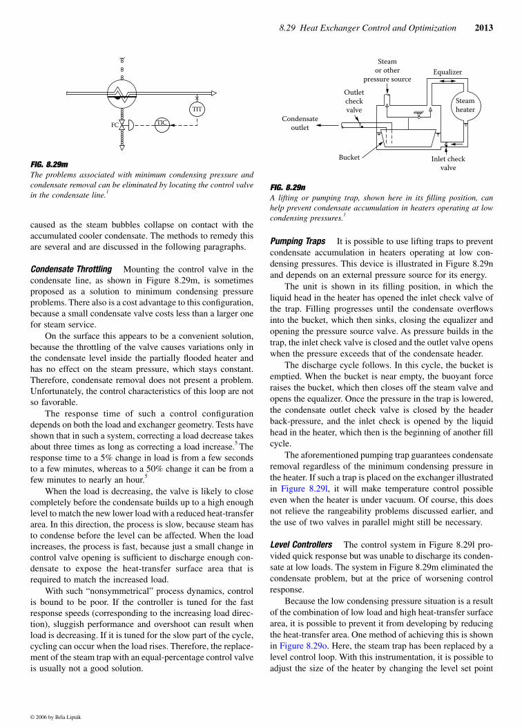
Pumping Traps It is possible to use lifting traps to preventcondensate accumulation in heaters operating at low con-densing pressures. This device is illustrated in Figure 8.29nand depends on an external pressure source for its energy.
The unit is shown in its filling position, in which theliquid head in the heater has opened the inlet check valve ofthe trap. Filling progresses until the condensate overflowsinto the bucket, which then sinks, closing the equalizer andopening the pressure source valve. As pressure builds in thetrap, the inlet check valve is closed and the outlet valve openswhen the pressure exceeds that of the condensate header.
The discharge cycle follows. In this cycle, the bucket isemptied. When the bucket is near empty, the buoyant forceraises the bucket, which then closes off the steam valve andopens the equalizer. Once the pressure in the trap is lowered,the condensate outlet check valve is closed by the headerback-pressure, and the inlet check is opened by the liquidhead in the heater, which then is the beginning of another fillcycle.
The aforementioned pumping trap guarantees condensateremoval regardless of the minimum condensing pressure inthe heater. If such a trap is placed on the exchanger illustratedin Figure 8.29l, it will make temperature control possibleeven when the heater is under vacuum. Of course, this doesnot relieve the rangeability problems discussed earlier, andthe use of two valves in parallel might still be necessary.
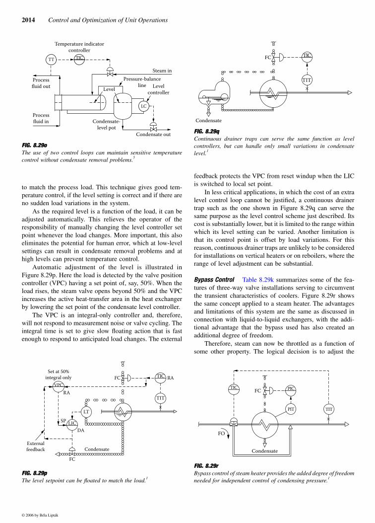
Level Controllers The control system in Figure 8.29l pro-vided quick response but was unable to discharge its conden-sate at low loads. The system in Figure 8.29m eliminated thecondensate problem, but at the price of worsening controlresponse.
Because the low condensing pressure situation is a resultof the combination of low load and high heat-transfer surfacearea, it is possible to prevent it from developing by reducingthe heat-transfer area. One method of achieving this is shownin Figure 8.29o. Here, the steam trap has been replaced by alevel control loop. With this instrumentation, it is possible toadjust the size of the heater by changing the level set point
FIG. 8.29mThe problems associated with minimum condensing pressure andcondensate removal can be eliminated by locating the control valvein the condensate line.1
TIC
TIT
FC
×
FIG. 8.29nA lifting or pumping trap, shown here in its filling position, canhelp prevent condensate accumulation in heaters operating at lowcondensing pressures.1
Steamheater
Inlet checkvalve
EqualizerSteam
or otherpressure source
Outletcheckvalve
Condensateoutlet
Bucket
© 2006 by Béla Lipták
2014 Control and Optimization of Unit Operations
to match the process load. This technique gives good tem-perature control, if the level setting is correct and if there areno sudden load variations in the system.
As the required level is a function of the load, it can beadjusted automatically. This relieves the operator of theresponsibility of manually changing the level controller setpoint whenever the load changes. More important, this alsoeliminates the potential for human error, which at low-levelsettings can result in condensate removal problems and athigh levels can prevent temperature control.
Automatic adjustment of the level is illustrated inFigure 8.29p. Here the load is detected by the valve positioncontroller (VPC) having a set point of, say, 50%. When theload rises, the steam valve opens beyond 50% and the VPCincreases the active heat-transfer area in the heat exchangerby lowering the set point of the condensate level controller.
The VPC is an integral-only controller and, therefore,will not respond to measurement noise or valve cycling. Theintegral time is set to give slow floating action that is fastenough to respond to anticipated load changes. The external
feedback protects the VPC from reset windup when the LICis switched to local set point.
In less critical applications, in which the cost of an extralevel control loop cannot be justified, a continuous drainertrap such as the one shown in Figure 8.29q can serve thesame purpose as the level control scheme just described. Itscost is substantially lower, but it is limited to the range withinwhich its level setting can be varied. Another limitation isthat its control point is offset by load variations. For thisreason, continuous drainer traps are unlikely to be consideredfor installations on vertical heaters or on reboilers, where therange of level adjustment can be substantial.
Bypass Control Table 8.29k summarizes some of the fea-tures of three-way valve installations serving to circumventthe transient characteristics of coolers. Figure 8.29r showsthe same concept applied to a steam heater. The advantagesand limitations of this system are the same as discussed inconnection with liquid-to-liquid exchangers, with the addi-tional advantage that the bypass used has also created anadditional degree of freedom.
Therefore, steam can now be throttled as a function ofsome other property. The logical decision is to adjust the
FIG. 8.29oThe use of two control loops can maintain sensitive temperaturecontrol without condensate removal problems.5
FIG. 8.29pThe level setpoint can be floated to match the load.1
Processfluid out
Processfluid in
Steam in
TIC
LC
TT
Temperature indicatorcontroller
Pressure-balanceline Level
controllerLevel
Condensate-level pot
Condensate out
TIC RAFC
TIT
VPC
LIC
LT
Set at 50%integral only
Externalfeedback
FC
DA
SP
RA
Condensate
FIG. 8.29qContinuous drainer traps can serve the same function as levelcontrollers, but can handle only small variations in condensatelevel.1
FIG. 8.29rBypass control of steam heater provides the added degree of freedomneeded for independent control of condensing pressure.1
TIC
TIT
FC
Condensate
×
PIC
PIT
FCTIC
TIT
FO
Condensate
×
© 2006 by Béla Lipták
8.29 Heat Exchanger Control and Optimization 2015
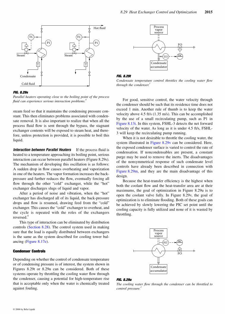
steam feed so that it maintains the condensing pressure con-stant. This then eliminates problems associated with conden-sate removal. It is also important to realize that when all theprocess fluid flow is sent through the bypass, the stagnantexchanger contents will be exposed to steam heat, and there-fore, unless protection is provided, it is possible to boil thisliquid.
Interaction between Parallel Heaters If the process fluid isheated to a temperature approaching its boiling point, seriousinteraction can occur between parallel heaters (Figure 8.29s).The mechanism of developing this oscillation is as follows:A sudden drop in flow causes overheating and vaporizationin one of the heaters. The vapor formation increases the back-pressure and further reduces the flow, eventually forcing allflow through the other “cold” exchanger, while the “hot”exchanger discharges slugs of liquid and vapor.
After a period of noise and vibration, when the “hot”exchanger has discharged all of its liquid, the back-pressuredrops and flow is resumed, drawing feed from the “cold”exchanger. This causes the “cold” exchanger to overheat, andthe cycle is repeated with the roles of the exchangersreversed.4
This type of interaction can be eliminated by distributioncontrols (Section 8.28). The control system used in makingsure that the load is equally distributed between exchangersis the same as the system described for cooling tower bal-ancing (Figure 8.17e).
Condenser Controls
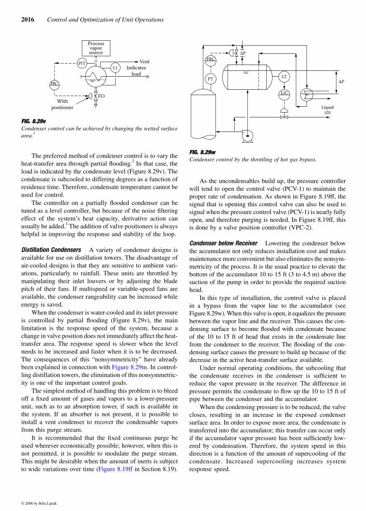
Depending on whether the control of condensate temperatureor of condensing pressure is of interest, the system shown inFigures 8.29t or 8.29u can be considered. Both of thesesystems operate by throttling the cooling water flow throughthe condenser, causing a potential for high-temperature risethat is acceptable only when the water is chemically treatedagainst fouling.
For good, sensitive control, the water velocity throughthe condenser should be such that its residence time does notexceed 1 min. Another rule of thumb is to keep the watervelocity above 4.5 ft/s (1.35 m/s). This can be accomplishedby the use of a small recirculating pump, such as P1 inFigure 8.13i. In this system, FSHL-3 detects the net forwardvelocity of the water. As long as it is under 4.5 ft/s, FSHL-3 will keep the recirculating pump running.
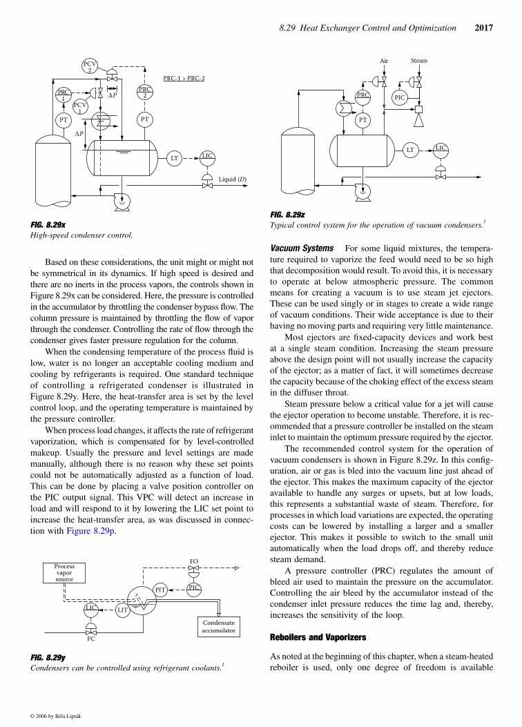
When it is not desirable to throttle the cooling water, thesystem illustrated in Figure 8.29v can be considered. Here,the exposed condenser surface is varied to control the rate ofcondensation. If noncondensables are present, a constantpurge may be used to remove the inerts. The disadvantagesof the nonsymmetrical response of such condensate levelcontrols have already been described in connection withFigure 8.29m, and they are the main disadvantage of thisdesign.
Because the heat-transfer efficiency is the highest whenboth the coolant flow and the heat-transfer area are at theirmaximums, the goal of optimization in Figure 8.29u is toopen the coolant valve fully. In Figure 8.29v, the goal ofoptimization is to eliminate flooding. Both of these goals canbe achieved by slowly lowering the PIC set point until thecooling capacity is fully utilized and none of it is wasted bythrottling.
FIG. 8.29sParallel heaters operating close to the boiling point of the processfluid can experience serious interaction problems.4
TC
P1
Hot fluid
T
Steam
TC
P1
T
Steam
Condensate
Cold fluid
× ×
FIG. 8.29tCondensate temperature control throttles the cooling water flowthrough the condenser.1
FIG. 8.29uThe cooling water flow through the condenser can be throttled tocontrol pressure.1
Processvaporsource
Condensateaccumulator
TICTIT
FO
×
Processvaporsource
Condensateaccumulator
FO
PIT PIC
© 2006 by Béla Lipták
2016 Control and Optimization of Unit Operations
The preferred method of condenser control is to vary theheat-transfer area through partial flooding.2 In that case, theload is indicated by the condensate level (Figure 8.29v). Thecondensate is subcooled to differing degrees as a function ofresidence time. Therefore, condensate temperature cannot beused for control.
The controller on a partially flooded condenser can betuned as a level controller, but because of the noise filteringeffect of the system’s heat capacity, derivative action canusually be added.2 The addition of valve positioners is alwayshelpful in improving the response and stability of the loop.
Distillation Condensers A variety of condenser designs isavailable for use on distillation towers. The disadvantage ofair-cooled designs is that they are sensitive to ambient vari-ations, particularly to rainfall. These units are throttled bymanipulating their inlet louvers or by adjusting the bladepitch of their fans. If multispeed or variable-speed fans areavailable, the condenser rangeability can be increased whileenergy is saved.
When the condenser is water-cooled and its inlet pressureis controlled by partial flooding (Figure 8.29v), the mainlimitation is the response speed of the system, because achange in valve position does not immediately affect the heat-transfer area. The response speed is slower when the levelneeds to be increased and faster when it is to be decreased.The consequences of this “nonsymmetricity” have alreadybeen explained in connection with Figure 8.29m. In control-ling distillation towers, the elimination of this nonsymmetric-ity is one of the important control goals.
The simplest method of handling this problem is to bleedoff a fixed amount of gases and vapors to a lower-pressureunit, such as to an absorption tower, if such is available inthe system. If an absorber is not present, it is possible toinstall a vent condenser to recover the condensable vaporsfrom this purge stream.
It is recommended that the fixed continuous purge beused wherever economically possible; however, when this isnot permitted, it is possible to modulate the purge stream.This might be desirable when the amount of inerts is subjectto wide variations over time (Figure 8.19ff in Section 8.19).
As the uncondensables build up, the pressure controllerwill tend to open the control valve (PCV-1) to maintain theproper rate of condensation. As shown in Figure 8.19ff, thesignal that is opening this control valve can also be used tosignal when the pressure control valve (PCV-1) is nearly fullyopen, and therefore purging is needed. In Figure 8.19ff, thisis done by a valve position controller (VPC-2).
Condenser below Receiver Lowering the condenser belowthe accumulator not only reduces installation cost and makesmaintenance more convenient but also eliminates the nonsym-metricity of the process. It is the usual practice to elevate thebottom of the accumulator 10 to 15 ft (3 to 4.5 m) above thesuction of the pump in order to provide the required suctionhead.
In this type of installation, the control valve is placedin a bypass from the vapor line to the accumulator (seeFigure 8.29w). When this valve is open, it equalizes the pressurebetween the vapor line and the receiver. This causes the con-densing surface to become flooded with condensate becauseof the 10 to 15 ft of head that exists in the condensate linefrom the condenser to the receiver. The flooding of the con-densing surface causes the pressure to build up because of thedecrease in the active heat-transfer surface available.
Under normal operating conditions, the subcooling thatthe condensate receives in the condenser is sufficient toreduce the vapor pressure in the receiver. The difference inpressure permits the condensate to flow up the 10 to 15 ft ofpipe between the condenser and the accumulator.
When the condensing pressure is to be reduced, the valvecloses, resulting in an increase in the exposed condensersurface area. In order to expose more area, the condensate istransferred into the accumulator; this transfer can occur onlyif the accumulator vapor pressure has been sufficiently low-ered by condensation. Therefore, the system speed in thisdirection is a function of the amount of supercooling of thecondensate. Increased supercooling increases systemresponse speed.
FIG. 8.29vCondenser control can be achieved by changing the wetted surfacearea.1
Processvaporsource
FO
PIT
PIC
L1Vent
Indicatesload
Withpositioner
FIG. 8.29wCondenser control by the throttling of hot gas bypass.
PRC
PT
LIC
LT
Liquid(D)
∆P
∆P
© 2006 by Béla Lipták
8.29 Heat Exchanger Control and Optimization 2017
Based on these considerations, the unit might or might notbe symmetrical in its dynamics. If high speed is desired andthere are no inerts in the process vapors, the controls shown inFigure 8.29x can be considered. Here, the pressure is controlledin the accumulator by throttling the condenser bypass flow. Thecolumn pressure is maintained by throttling the flow of vaporthrough the condenser. Controlling the rate of flow through thecondenser gives faster pressure regulation for the column.
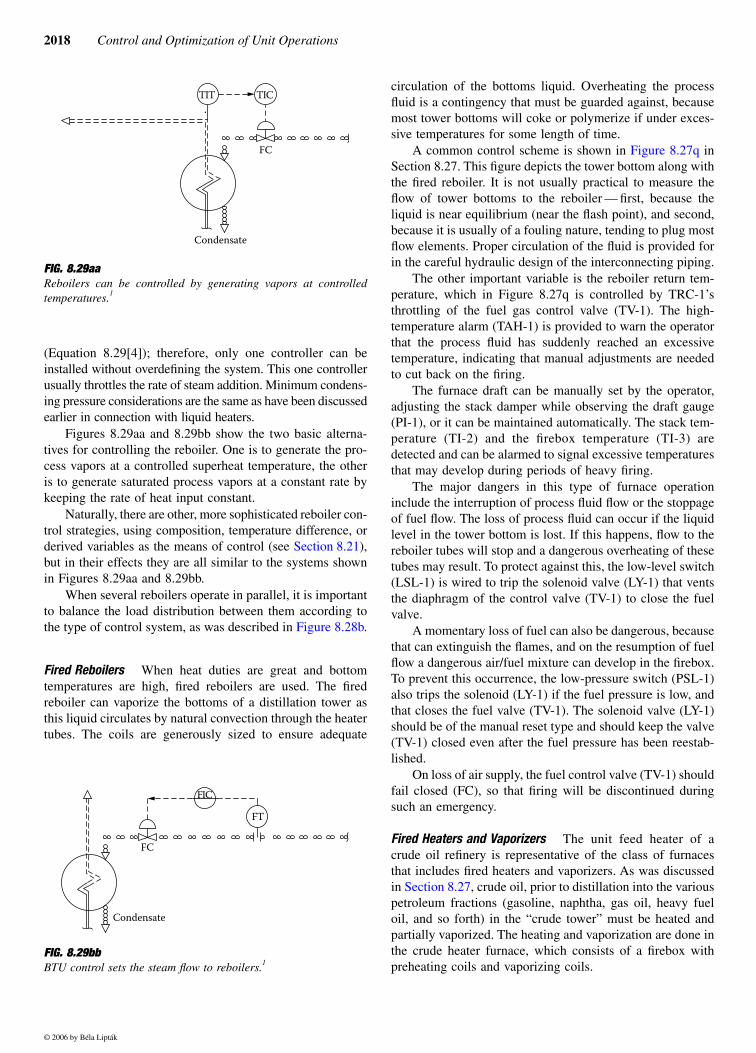
When the condensing temperature of the process fluid islow, water is no longer an acceptable cooling medium andcooling by refrigerants is required. One standard techniqueof controlling a refrigerated condenser is illustrated inFigure 8.29y. Here, the heat-transfer area is set by the levelcontrol loop, and the operating temperature is maintained bythe pressure controller.
When process load changes, it affects the rate of refrigerantvaporization, which is compensated for by level-controlledmakeup. Usually the pressure and level settings are mademanually, although there is no reason why these set pointscould not be automatically adjusted as a function of load.This can be done by placing a valve position controller onthe PIC output signal. This VPC will detect an increase inload and will respond to it by lowering the LIC set point toincrease the heat-transfer area, as was discussed in connec-tion with Figure 8.29p.
Vacuum Systems For some liquid mixtures, the tempera-ture required to vaporize the feed would need to be so highthat decomposition would result. To avoid this, it is necessaryto operate at below atmospheric pressure. The commonmeans for creating a vacuum is to use steam jet ejectors.These can be used singly or in stages to create a wide rangeof vacuum conditions. Their wide acceptance is due to theirhaving no moving parts and requiring very little maintenance.
Most ejectors are fixed-capacity devices and work bestat a single steam condition. Increasing the steam pressureabove the design point will not usually increase the capacityof the ejector; as a matter of fact, it will sometimes decreasethe capacity because of the choking effect of the excess steamin the diffuser throat.
Steam pressure below a critical value for a jet will causethe ejector operation to become unstable. Therefore, it is rec-ommended that a pressure controller be installed on the steaminlet to maintain the optimum pressure required by the ejector.
The recommended control system for the operation ofvacuum condensers is shown in Figure 8.29z. In this config-uration, air or gas is bled into the vacuum line just ahead ofthe ejector. This makes the maximum capacity of the ejectoravailable to handle any surges or upsets, but at low loads,this represents a substantial waste of steam. Therefore, forprocesses in which load variations are expected, the operatingcosts can be lowered by installing a larger and a smallerejector. This makes it possible to switch to the small unitautomatically when the load drops off, and thereby reducesteam demand.
A pressure controller (PRC) regulates the amount ofbleed air used to maintain the pressure on the accumulator.Controlling the air bleed by the accumulator instead of thecondenser inlet pressure reduces the time lag and, thereby,increases the sensitivity of the loop.
Reboilers and Vaporizers
As noted at the beginning of this chapter, when a steam-heatedreboiler is used, only one degree of freedom is available
FIG. 8.29xHigh-speed condenser control.
FIG. 8.29yCondensers can be controlled using refrigerant coolants.1
PRC1
PT
PCV1
PCV2
LT
∆P
∆P
LIC
Liquid (D)
PRC
PT
2
PRC-1 > PRC-2
Processvaporsource
Condensateaccumulator
FC
PIT PIC
LIC LIT
FO
FIG. 8.29z Typical control system for the operation of vacuum condensers.1
LICLT
PRC
PT
Air
PIC
Steam
© 2006 by Béla Lipták
2018 Control and Optimization of Unit Operations
(Equation 8.29[4]); therefore, only one controller can beinstalled without overdefining the system. This one controllerusually throttles the rate of steam addition. Minimum condens-ing pressure considerations are the same as have been discussedearlier in connection with liquid heaters.
Figures 8.29aa and 8.29bb show the two basic alterna-tives for controlling the reboiler. One is to generate the pro-cess vapors at a controlled superheat temperature, the otheris to generate saturated process vapors at a constant rate bykeeping the rate of heat input constant.
Naturally, there are other, more sophisticated reboiler con-trol strategies, using composition, temperature difference, orderived variables as the means of control (see Section 8.21),but in their effects they are all similar to the systems shownin Figures 8.29aa and 8.29bb.
When several reboilers operate in parallel, it is importantto balance the load distribution between them according tothe type of control system, as was described in Figure 8.28b.
Fired Reboilers When heat duties are great and bottomtemperatures are high, fired reboilers are used. The firedreboiler can vaporize the bottoms of a distillation tower asthis liquid circulates by natural convection through the heatertubes. The coils are generously sized to ensure adequate
circulation of the bottoms liquid. Overheating the processfluid is a contingency that must be guarded against, becausemost tower bottoms will coke or polymerize if under exces-sive temperatures for some length of time.
A common control scheme is shown in Figure 8.27q inSection 8.27. This figure depicts the tower bottom along withthe fired reboiler. It is not usually practical to measure theflow of tower bottoms to the reboiler — first, because theliquid is near equilibrium (near the flash point), and second,because it is usually of a fouling nature, tending to plug mostflow elements. Proper circulation of the fluid is provided forin the careful hydraulic design of the interconnecting piping.
The other important variable is the reboiler return tem-perature, which in Figure 8.27q is controlled by TRC-1’sthrottling of the fuel gas control valve (TV-1). The high-temperature alarm (TAH-1) is provided to warn the operatorthat the process fluid has suddenly reached an excessivetemperature, indicating that manual adjustments are neededto cut back on the firing.
The furnace draft can be manually set by the operator,adjusting the stack damper while observing the draft gauge(PI-1), or it can be maintained automatically. The stack tem-perature (TI-2) and the firebox temperature (TI-3) aredetected and can be alarmed to signal excessive temperaturesthat may develop during periods of heavy firing.
The major dangers in this type of furnace operationinclude the interruption of process fluid flow or the stoppageof fuel flow. The loss of process fluid can occur if the liquidlevel in the tower bottom is lost. If this happens, flow to thereboiler tubes will stop and a dangerous overheating of thesetubes may result. To protect against this, the low-level switch(LSL-1) is wired to trip the solenoid valve (LY-1) that ventsthe diaphragm of the control valve (TV-1) to close the fuelvalve.
A momentary loss of fuel can also be dangerous, becausethat can extinguish the flames, and on the resumption of fuelflow a dangerous air/fuel mixture can develop in the firebox.To prevent this occurrence, the low-pressure switch (PSL-1)also trips the solenoid (LY-1) if the fuel pressure is low, andthat closes the fuel valve (TV-1). The solenoid valve (LY-1)should be of the manual reset type and should keep the valve(TV-1) closed even after the fuel pressure has been reestab-lished.
On loss of air supply, the fuel control valve (TV-1) shouldfail closed (FC), so that firing will be discontinued duringsuch an emergency.
Fired Heaters and Vaporizers The unit feed heater of acrude oil refinery is representative of the class of furnacesthat includes fired heaters and vaporizers. As was discussedin Section 8.27, crude oil, prior to distillation into the variouspetroleum fractions (gasoline, naphtha, gas oil, heavy fueloil, and so forth) in the “crude tower” must be heated andpartially vaporized. The heating and vaporization are done inthe crude heater furnace, which consists of a firebox withpreheating coils and vaporizing coils.
FIG. 8.29aaReboilers can be controlled by generating vapors at controlledtemperatures.1
FIG. 8.29bbBTU control sets the steam flow to reboilers.1
TIT TIC
Condensate
FC
⋅
FIC
Condensate
FC
FT
© 2006 by Béla Lipták
8.29 Heat Exchanger Control and Optimization 2019
The heating is usually done in coils in the convectionsection of the furnace. The convection section is the portionof the coils that does not see the flame but that is exposed tothe hot flue gases on their way to the stack. The vaporizingtakes place at the end of each pass in the radiant section ofthe furnace (where the coils are exposed to the flame and theluminous walls of the firebox).
The partially vaporized effluent then enters the crudetower, where it flashes and is distilled into the desired “cuts.”Other process heaters that fall into this category are refineryvacuum tower preheaters, reformer heaters, hydrocrackerheaters, and dewaxing unit furnaces.
The prime control tasks in this process are
1. Flow control of feed to the unit2. Proper splitting of flow into the parallel paths through
the furnace to prevent overheating of any one stream,which could result in coking
3. Supplying the correct amount of heat to the crudetower
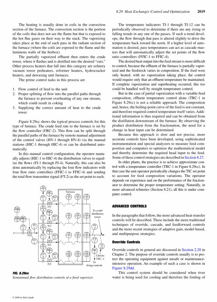
Figure 8.29cc shows the typical process controls for thistype of furnace. The crude feed rate to the furnace is set bythe flow controller (FRC-2). This flow can be split throughthe parallel paths of the furnace by remote manual adjustmentof the control valves (HV-1 through HV-4) via the manualstations (HIC-1 through HIC-4) or can be distributed auto-matically.
In this manual control configuration, the operator manu-ally adjusts (HIC-1 to HIC-4) the distribution valves to equal-ize the flows (FI-1 through FI-4). Naturally, this can also bedone automatically by replacing the four flow indicators withfour flow ratio controllers (FFIC-1 to FFIC-4) and sendingthe total flow transmitter signal (FT-2) as the set point to each.
The temperature indicators TI-1 through TI-12 can beperiodically observed to determine if there are any rising orfalling trends in any one of the passes. If such a trend devel-ops, the flow through that pass is altered slightly to drive thetemperature back toward the norm. If a higher level of auto-mation is desired, pass temperatures can act as cascade mas-ters that will automatically adjust the set points of the flowratio controllers (FFIC-1 to FFIC-4).
The desired heat output into the feed stream is more difficultto control, because the effluent of the furnace is partially vapor-ized and the feedstock varies in composition. If the feed wereonly heated, with no vaporization taking place, the controlwould require only that an effluent temperature be maintained.If complete vaporization and superheating occurred, this toocould be handled well by straight temperature control.
But in the case of partial vaporization with a variable-feedcomposition, effluent temperature control alone (TRC-1 inFigure 8.29cc) is not a reliable approach. The compositionand, hence, the boiling-point curve of the feed is not constant,and therefore required control temperature itself varies. Addi-tional information is thus required and can be obtained fromthe distillation downstream of the furnace. By observing theproduct distribution from the fractionation, the need for achange in heat input can be determined.
Because this approach is slow and not precise, moreaccurate controls have been developed, using sophisticatedinstrumentation and special analyzers to measure feed com-position and computers to optimize the mathematical modeland thereby determine the required head input to the feed.Some of these control strategies are described in Section 8.27.
In older plants, the practice is to achieve approximate con-trol with a temperature controller (TRC-1 in Figure 8.29cc). Inthat case the unit operator periodically changes the TIC set pointto account for feed composition variations. The operatordepends on experience and on the performance of the fraction-ator to determine the proper temperature setting. Naturally, inmore advanced refineries (Section 8.21), all this is under com-puter control.
ADVANCED CONTROLS
In the paragraphs that follow, the more advanced heat-transfercontrols will be described. These include the more traditionaltechniques of override, cascade, and feedforward controlsand the more recent strategies of adaptive gain, model-based,and multipurpose strategies.
Override Controls
Override controls in general are discussed in Section 2.28 inChapter 2. The purpose of override controls usually is to pro-tect the operating equipment against unsafe or maintenance-intensive operation. An example of such a case is shown inFigure 8.29dd.
This control system should be considered when riverwater is being used for cooling and therefore the fouling of
FIG. 8.29ccSemiannual flow distribution controls of a fired vaporizer.
TI1
FI1
FT1
HV1
HIC1 TI
2TI3
TI4
TI5
TI6
PI2
TT1
TI13
TRC1
TI7
TI8
TI9
TI10
TI11
TI12
Furnace
ChecksTRC–1
Tofiring controls
To crudedistillation
tower
FAL2
PI1
FV1
FRC2
FT2
FSL2
FI2
FT2
HV2
HIC2
FI3
FT3
HV3
HIC3
FI4
FT4
HV4
HIC4
FO
FO
FO
FO
FO
© 2006 by Béla Lipták
2020 Control and Optimization of Unit Operations
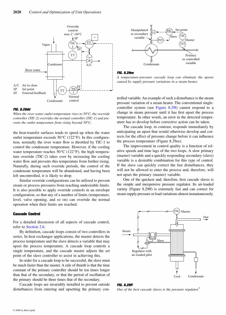
the heat-transfer surfaces tends to speed up when the wateroutlet temperature exceeds 50°C (122°F). In this configura-tion, normally the river water flow is throttled by TIC-1 tocontrol the condensate temperature. However, if the coolingwater temperature reaches 50°C (122°F), the high tempera-ture override (TIC-2) takes over by increasing the coolingwater flow and prevents this temperature from further rising.Naturally, during such override periods, the control of thecondensate temperature will be abandoned, and having beenleft uncontrolled, it is likely to drop.
Similar override configurations can be utilized to preventsteam or process pressures from reaching undesirable limits.It is also possible to apply override controls in an envelopeconfiguration, so that any of a number of limits (temperature,level, valve opening, and so on) can override the normaloperation when their limits are reached.
Cascade Control
For a detailed discussion of all aspects of cascade control,refer to Section 2.6.
By definition, cascade loops consist of two controllers inseries. In heat exchanger applications, the master detects theprocess temperature and the slave detects a variable that mayupset the process temperature. A cascade loop controls asingle temperature, and the cascade master adjusts the setpoint of the slave controller to assist in achieving this.
In order for a cascade loop to be successful, the slave mustbe much faster than the master. A rule of thumb is that the timeconstant of the primary controller should be ten times longerthan that of the secondary, or that the period of oscillation ofthe primary should be three times that of the secondary.
Cascade loops are invariably installed to prevent outsidedisturbances from entering and upsetting the primary con-
trolled variable. An example of such a disturbance is the steampressure variation of a steam heater. The conventional single-controller system (see Figure 8.29l) cannot respond to achange in steam pressure until it has first upset the processtemperature. In other words, an error in the detected temper-ature has to develop before corrective action can be taken.
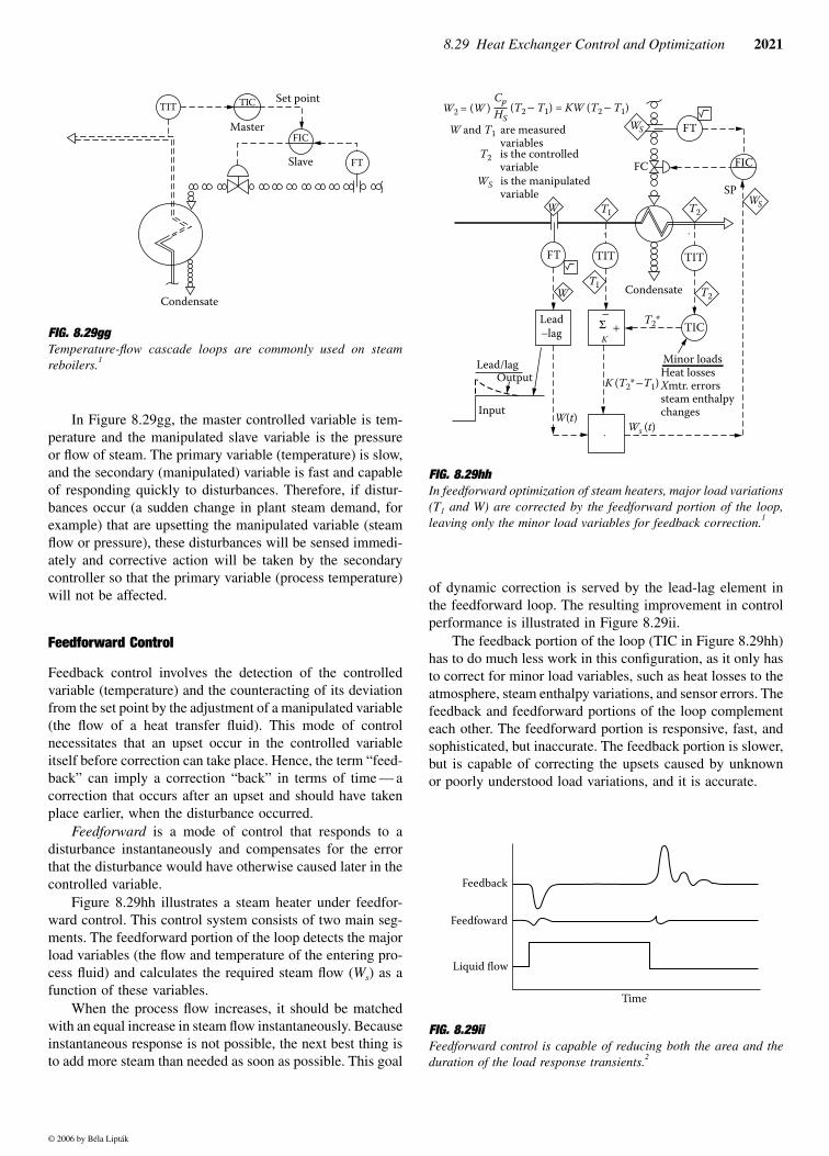
The cascade loop, in contrast, responds immediately byanticipating an upset that would otherwise develop and cor-rects for the effect of pressure change before it can influencethe process temperature (Figure 8.29ee).
The improvement in control quality is a function of rel-ative speeds and time lags of the two loops. A slow primary(master) variable and a quickly responding secondary (slave)variable is a desirable combination for this type of control.If the slave can quickly correct the fast disturbances, theywill not be allowed to enter the process and, therefore, willnot upset the primary (master) variable.
One of the quickest and, therefore, best cascade slaves isthe simple and inexpensive pressure regulator. Its air-loadedvariety (Figure 8.29ff) is extremely fast and can correct forsteam supply pressure or load variations almost instantaneously.
FIG. 8.29ddWhen the river water outlet temperature rises to 50°C, the overridecontroller (TIC-2) overrides the normal controller (TIC-1) and pre-vents the outlet temperature from rising beyond 50°C.
TIC
TT
SP
1
Condenser
River water
Vapor
Condensate
A/C Air to closeSP Set pointEF External feedback
Normalcontrol
EF
EF
FY
A/C
Overridecontrol
max.T =50°C<
TT
TIC2
FIG. 8.29ee A temperature-pressure cascade loop can eliminate the upsetscaused by supply pressure variations in a steam heater.
FIG. 8.29ffOne of the best cascade slaves is the pressure regulator.6
PIT
Manipulatedor secondary
variable TICPIC
TIT
Set point
SlaveMaster
Condensate
Primaryor controlled
variable
TIC Master
Steam
Slave
Cool Condensate
Regulator withair-loaded pilot
Hot
© 2006 by Béla Lipták
8.29 Heat Exchanger Control and Optimization 2021
In Figure 8.29gg, the master controlled variable is tem-perature and the manipulated slave variable is the pressureor flow of steam. The primary variable (temperature) is slow,and the secondary (manipulated) variable is fast and capableof responding quickly to disturbances. Therefore, if distur-bances occur (a sudden change in plant steam demand, forexample) that are upsetting the manipulated variable (steamflow or pressure), these disturbances will be sensed immedi-ately and corrective action will be taken by the secondarycontroller so that the primary variable (process temperature)will not be affected.
Feedforward Control
Feedback control involves the detection of the controlledvariable (temperature) and the counteracting of its deviationfrom the set point by the adjustment of a manipulated variable(the flow of a heat transfer fluid). This mode of controlnecessitates that an upset occur in the controlled variableitself before correction can take place. Hence, the term “feed-back” can imply a correction “back” in terms of time — acorrection that occurs after an upset and should have takenplace earlier, when the disturbance occurred.
Feedforward is a mode of control that responds to adisturbance instantaneously and compensates for the errorthat the disturbance would have otherwise caused later in thecontrolled variable.
Figure 8.29hh illustrates a steam heater under feedfor-ward control. This control system consists of two main seg-ments. The feedforward portion of the loop detects the majorload variables (the flow and temperature of the entering pro-cess fluid) and calculates the required steam flow (Ws) as afunction of these variables.
When the process flow increases, it should be matchedwith an equal increase in steam flow instantaneously. Becauseinstantaneous response is not possible, the next best thing isto add more steam than needed as soon as possible. This goal
of dynamic correction is served by the lead-lag element inthe feedforward loop. The resulting improvement in controlperformance is illustrated in Figure 8.29ii.
The feedback portion of the loop (TIC in Figure 8.29hh)has to do much less work in this configuration, as it only hasto correct for minor load variables, such as heat losses to theatmosphere, steam enthalpy variations, and sensor errors. Thefeedback and feedforward portions of the loop complementeach other. The feedforward portion is responsive, fast, andsophisticated, but inaccurate. The feedback portion is slower,but is capable of correcting the upsets caused by unknownor poorly understood load variations, and it is accurate.
FIG. 8.29ggTemperature-flow cascade loops are commonly used on steamreboilers.1
TIC
FIC
FT
TIT
Condensate
Slave
Set point
Master
FIG. 8.29hhIn feedforward optimization of steam heaters, major load variations(T1 and W) are corrected by the feedforward portion of the loop,leaving only the minor load variables for feedback correction.1
FIG. 8.29iiFeedforward control is capable of reducing both the area and theduration of the load response transients.2
TIT
FC
TIT
FT
FT
W
WS
TI
FIC
SP
TIC
WS
W
K
TI
T2
T2*
T2
Condensate
Minor loads
Lead−lag
Lead/lagOutput
Input
⋅
Heat lossesXmtr. errorssteam enthalpychangesW(t)
Ws (t)
K (T2* −T1)
W2 = (W )CpHS
(T2 − T1) = KW (T2 − T1)
W and T1 are measured variables
T2 is the controlled variableWS is the manipulated variable
Σ−
+
⋅ ⋅
Feedback
Feedfoward
Liquid flow
Time
© 2006 by Béla Lipták
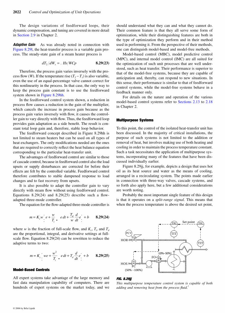
2022 Control and Optimization of Unit Operations
The design variations of feedforward loops, theirdynamic compensation, and tuning are covered in more detailin Section 2.9 in Chapter 2.
Adaptive Gain As was already noted in connection withFigure 8.29l, the heat-transfer process is a variable gain pro-cess. The steady-state gain of a steam heater process is
8.29(23)
Therefore, the process gain varies inversely with the pro-cess flow (W). If the temperature rise (T2 − T1) is also variable,even the use of an equal-percentage valve cannot correct forthis nonlinearity in the process. In that case, the only way tokeep the process gain constant is to use the feedforwardsystem shown in Figure 8.29hh.
In the feedforward control system shown, a reduction inprocess flow causes a reduction in the gain of the multiplier,which cancels the increase in process gain because as theprocess gain varies inversely with flow, it causes the control-ler gain to vary directly with flow. Thus, the feedforward loopprovides gain adaptation as a side benefit. The result is con-stant total loop gain and, therefore, stable loop behavior.
The feedforward concept described in Figure 8.29hh isnot limited to steam heaters but can be used on all types ofheat exchangers. The only modifications needed are the onesthat are required to correctly reflect the heat balance equationcorresponding to the particular heat-transfer unit.
The advantages of feedforward control are similar to thoseof cascade control, because in feedforward control also the loadupsets or supply disturbances are corrected for before theireffects are felt by the controlled variable. Feedforward controltherefore contributes to stable dampened response to loadchanges and to fast recovery from upsets.
It is also possible to adapt the controller gain to varydirectly with steam flow without using feedforward control.Equations 8.29(24) and 8.29(25) describe such a flow-adapted three-mode controller.
The equation for the flow-adapted three-mode controller is
8.29(24)
where w is the fraction of full-scale flow, and Kc, Ti, and Td
are the proportional, integral, and derivative settings at full-scale flow. Equation 8.29(24) can be rewritten to reduce theadaptive terms to two:
8.29(25)
Model-Based Controls
All expert systems take advantage of the large memory andfast data manipulation capability of computers. There arehundreds of expert systems on the market today, and we
should understand what they can and what they cannot do.Their common feature is that they all serve some form ofoptimization, while their distinguishing features are both inthe type of optimization they perform and in their methodused in performing it. From the perspective of their methods,one can distinguish model-based and model-free methods.
Model-based control (MBC), model predictive control(MPC), and internal model control (IMC) are all suited forthe optimization of such unit processes that are well under-stood, such as heat transfer. Their performance is superior tothat of the model-free systems, because they are capable ofanticipation and, thereby, can respond to new situations. Inthis sense, their performance is similar to that of feedforwardcontrol systems, while the model-free systems behave in afeedback manner only.
For details on the nature and operation of the variousmodel-based control systems refer to Sections 2.13 to 2.18in Chapter 2.
Multipurpose Systems
To this point, the control of the isolated heat-transfer unit hasbeen discussed. In the majority of critical installations, thepurpose of such systems is not limited to the addition orremoval of heat, but involves making use of both heating andcooling in order to maintain the process temperature constant.Such a task necessitates the application of multipurpose sys-tems, incorporating many of the features that have been dis-cussed individually earlier.
Figure 8.29jj, for example, depicts a design that uses hotoil as its heat source and water as the means of cooling,arranged in a recirculating system. The points made earlierin connection with three-way valves, cascade systems, andso forth also apply here, but a few additional considerationsare worth noting.
Probably the most important single feature of this designis that it operates on a split-range signal. This means thatwhen the process temperature is above the desired set point,
dT dW Hs WCps2 = .
m K w ewT
e dtT
wddt
e bci
d= + +.
...
..+.
m K wewT
e dt Tddt
e bci
d= + +.
...
..+.
2
FIG. 8.29jj This multipurpose temperature control system is capable of bothadding and removing heat from the process fluid.1
PCV
HOR
HOS
FO
FC(50% −100%)
(0%−50%)
Set pointTIC TIC
TIT
TIT
© 2006 by Béla Lipták
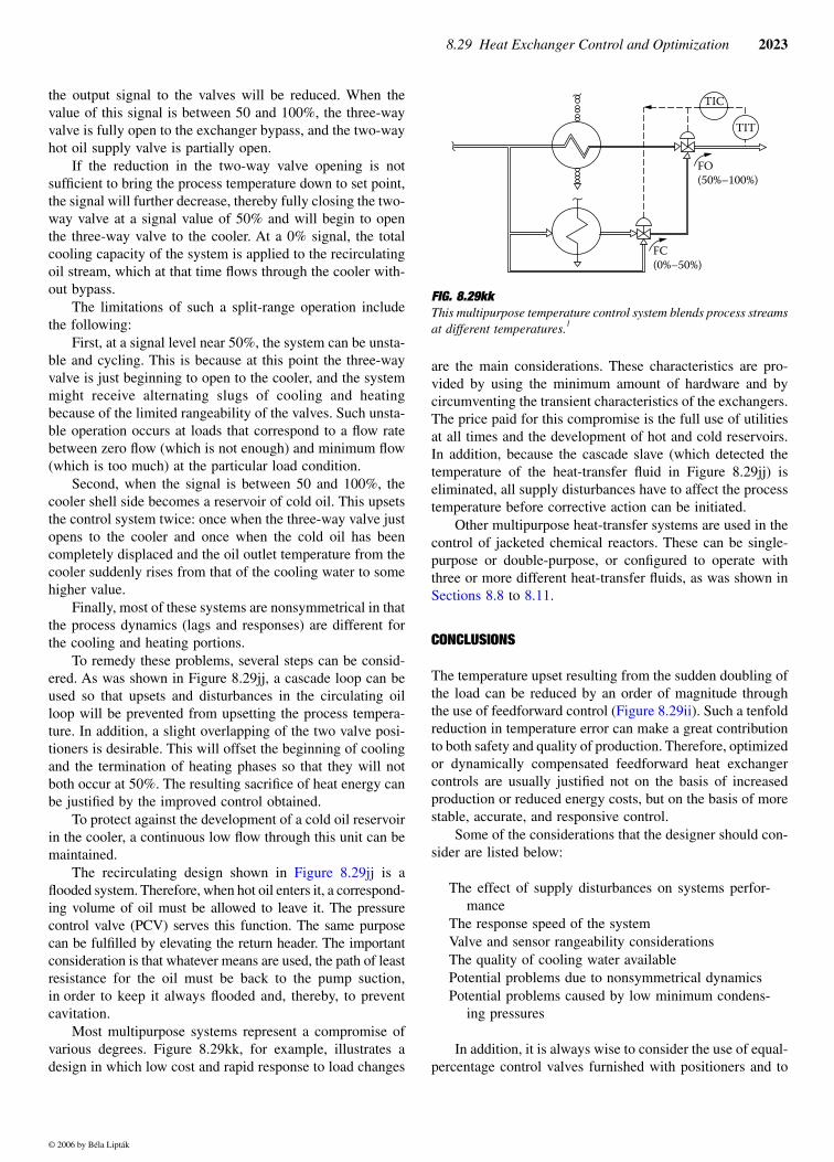
8.29 Heat Exchanger Control and Optimization 2023
the output signal to the valves will be reduced. When thevalue of this signal is between 50 and 100%, the three-wayvalve is fully open to the exchanger bypass, and the two-wayhot oil supply valve is partially open.
If the reduction in the two-way valve opening is notsufficient to bring the process temperature down to set point,the signal will further decrease, thereby fully closing the two-way valve at a signal value of 50% and will begin to openthe three-way valve to the cooler. At a 0% signal, the totalcooling capacity of the system is applied to the recirculatingoil stream, which at that time flows through the cooler with-out bypass.
The limitations of such a split-range operation includethe following:
First, at a signal level near 50%, the system can be unsta-ble and cycling. This is because at this point the three-wayvalve is just beginning to open to the cooler, and the systemmight receive alternating slugs of cooling and heatingbecause of the limited rangeability of the valves. Such unsta-ble operation occurs at loads that correspond to a flow ratebetween zero flow (which is not enough) and minimum flow(which is too much) at the particular load condition.
Second, when the signal is between 50 and 100%, thecooler shell side becomes a reservoir of cold oil. This upsetsthe control system twice: once when the three-way valve justopens to the cooler and once when the cold oil has beencompletely displaced and the oil outlet temperature from thecooler suddenly rises from that of the cooling water to somehigher value.
Finally, most of these systems are nonsymmetrical in thatthe process dynamics (lags and responses) are different forthe cooling and heating portions.
To remedy these problems, several steps can be consid-ered. As was shown in Figure 8.29jj, a cascade loop can beused so that upsets and disturbances in the circulating oilloop will be prevented from upsetting the process tempera-ture. In addition, a slight overlapping of the two valve posi-tioners is desirable. This will offset the beginning of coolingand the termination of heating phases so that they will notboth occur at 50%. The resulting sacrifice of heat energy canbe justified by the improved control obtained.
To protect against the development of a cold oil reservoirin the cooler, a continuous low flow through this unit can bemaintained.
The recirculating design shown in Figure 8.29jj is aflooded system. Therefore, when hot oil enters it, a correspond-ing volume of oil must be allowed to leave it. The pressurecontrol valve (PCV) serves this function. The same purposecan be fulfilled by elevating the return header. The importantconsideration is that whatever means are used, the path of leastresistance for the oil must be back to the pump suction,in order to keep it always flooded and, thereby, to preventcavitation.
Most multipurpose systems represent a compromise ofvarious degrees. Figure 8.29kk, for example, illustrates adesign in which low cost and rapid response to load changes
are the main considerations. These characteristics are pro-vided by using the minimum amount of hardware and bycircumventing the transient characteristics of the exchangers.The price paid for this compromise is the full use of utilitiesat all times and the development of hot and cold reservoirs.In addition, because the cascade slave (which detected thetemperature of the heat-transfer fluid in Figure 8.29jj) iseliminated, all supply disturbances have to affect the processtemperature before corrective action can be initiated.
Other multipurpose heat-transfer systems are used in thecontrol of jacketed chemical reactors. These can be single-purpose or double-purpose, or configured to operate withthree or more different heat-transfer fluids, as was shown inSections 8.8 to 8.11.
CONCLUSIONS
The temperature upset resulting from the sudden doubling ofthe load can be reduced by an order of magnitude throughthe use of feedforward control (Figure 8.29ii). Such a tenfoldreduction in temperature error can make a great contributionto both safety and quality of production. Therefore, optimizedor dynamically compensated feedforward heat exchangercontrols are usually justified not on the basis of increasedproduction or reduced energy costs, but on the basis of morestable, accurate, and responsive control.
Some of the considerations that the designer should con-sider are listed below:
The effect of supply disturbances on systems perfor-mance
The response speed of the systemValve and sensor rangeability considerationsThe quality of cooling water availablePotential problems due to nonsymmetrical dynamicsPotential problems caused by low minimum condens-
ing pressures
In addition, it is always wise to consider the use of equal-percentage control valves furnished with positioners and to
FIG. 8.29kkThis multipurpose temperature control system blends process streamsat different temperatures.1
TIC
TIT
FC(0%–50%)
FO(50%–100%)
© 2006 by Béla Lipták
2024 Control and Optimization of Unit Operations
evaluate the advisability of using cascade, feedforward, ormodel-based advanced controls.
References
1. Lipták, B. G., “Control of Heat Exchangers,” British Chemical Engi-neering and Process Technology, Vol. 17, No. 7/8, p. 637, July/August1972.
2. Shinskey, F. G., Process Control Systems, 2nd edition, New York:McGraw-Hill, 1979, pp. 186, 227.
3. Shinskey, F. G., Controlling Multivariable Processes, Research Trian-gle Park, NC: ISA, 1981, p. 74.
4. Shinskey, F. G., Controlling Unstable Processes, Publication 413–4,The Foxboro Co.
5. Mathur, J., “Performance of Steam Heat-Exchangers,” Chemical Engi-neering, September 3, 1973.
6. Driskell, L. R., Control Valve Selection and Sizing, Research TrianglePark, NC: ISA, 1983.
Bibliography
Astrom, K. J., PID Controllers: Theory, Design, and Tuning, 2nd edition,Research Triangle Park, NC: Instrument Society of America, 1995.
Åström, K. J. and Hägglund, T., PID Controllers: Theory, Design and Tuning,Research Triangle Park, NC: Instrument Society of America, 1995.
Bailey, E. G., “How to Save Coal,” Bulletin No. 41, Wickliffe, OH: BaileyMeter Company, April 1918.
Batur, C., Sharpless, R. B., Duval, W. M. B., Rosenthal, B. N., and Singh,N. B., “Adaptive Temperature Profile Control of a Multizone CrystalGrowth Furnace,” Proceedings of the American Society of MechanicalEngineers, Dallas, TX, November 1990.
Boyle, W. E. and Hoyt, P. R., “Experimental Application of CombustionControls to a Process Heater,” Annual ISA Conference, September13–17, 1948.
Dukelow, S. G., “Energy Conservation through Instrumentation,” Universityof Houston Energy Conservation Seminar, February 7, 1975.
Dukelow, S. G., “Fired Process Heaters,” presented at ISA/CHEMPID, April1980.
Dukelow, S. G., “How Control Improvements Save Process Heater Fuel,”1979 Conference on Industrial Energy Conservation Technology,Houston, TX, April 23, 1979.
Edwards, D., “From LR to PC: Recent Developments in Furnace ControlSystems,” Metals and Materials, October 1990.
Forman, E. R., “Control Dynamics in Heat Transfer,” Chemical Engineering,January 3, 1966.
Gibson, J. E., Nonlinear Automatic Control, New York: McGraw-Hill BookCo., 1963.
Goodwin, G. C., Graebe, S. F., and Salgado, M. E., Control System Design,Prentice-Hall, 2001.
Hesselgreaves, J. E., Compact Heat Exchangers, New York: Pergamon Press,2001.
Hugo, A., “Limitations of Model Predictive Controllers,” Hydrocarbon Pro-cessing, January 2000.
Johnson, R. K., “Modern Approach to Process Heater Control Systems,”Parkersburg-Marietta ISA Section, Parkersburg, WV, February 8, 1977.
Kakac, S. et al., Heat Exchangers: Selection, Rating, and Thermal Design,2nd edition, Boca Raton, FL: CRC Press, 2002.
Khalil, E. E., Modeling of Furnaces and Combustors, Abacus Press, 1982.Kuppan, T., Heat Exchanger Design Handbook, New York: Marcel Dekker,
2000.Levine, W., The Control Handbook, Boca Raton, FL: CRC Press, 1996.Lipták, B. G., “Process Control Trends,”, Control, March, May, and July,
2004.Lipták, B. G., “Control of Heat Exchangers,” British Chemical Engineering,
July 1972.Luyben, W. L. and Tyreus, B. D., Plantwide Process Control, New York:
McGraw-Hill, 1998.Mathur, J., “Performance of Stream Heat-Exchangers,” Chemical Engineer-
ing, September 3, 1973.McKetta, J. J., Unit Operations Handbook, Volume 1, Mass Transfer, New
York: Marcel Dekker.McMillan, G. K., Tuning and Control Loop Performance, 3rd edition,
Research Triangle Park, NC: ISA, 1994.McMillan, G. K., Process Industrial Instruments and Control Handbook,
New York: McGraw-Hill, 1999.Ociai, S., “Creating Process Control Parameters from Steady-State Data,”
ISA Transactions, Volume 36, 1998.Omata, S., Yamamoto, T., Maruyama, H., and Hotta, M., “Adaptive Control
of a Furnace Temperature by Using a Microcomputer,” Proceedingsof the 28th Society of Instrument and Control Engineers, Tokyo, July1989.
Perry, R. H., Chemical Engineers Handbook, 7th edition, New York:McGraw-Hill Book Co., 1997.
Ruel, M. “Loop Optimization: How to Tune a Loop,” Control Magazine,Vol. 12, No. 5 (May 1999), pp. 83–86.
Seborg, D. E., Edgar, T. F., and Mellichamp, D. A., Process Dynamics andControl, 2nd edition, New York: John Wiley & Sons Inc., 2003.
Shinskey, F. G., “Feedforward Control Applied,” ISA Journal, November1963.
Shinskey, F. G., Process Control Systems, 4th edition, New York: McGraw-Hill, 1996.
Shinskey, F. G., Process Control Systems: Application, Design and Tuning,4th edition, New York: McGraw-Hill, 1998.
Skogestad, S. and Postlethwaite, I., Multivariable Feedback Control, NewYork: John Wiley & Sons Inc., 1996.
Waller, M. H., “Measurement and Control of Paper Stock Consistency,” ISAConference in Houston, TX, October 1992.
© 2006 by Béla Lipták


![---Activator and its modifications[14.9.16=8.29 pm]](https://img.pdfslide.us/doc/110x75/587173911a28ab230b8b4897/-activator-and-its-modifications14916829-pm.jpg)