Embed Size (px)
Citation preview

WATER RESOURCES OF SOUTH AFRICA, 2012 STUDY (WR2012)
WRSM/Pitman Theory Manual
Report to the Water Research Commission
by
AK Bailey and WV Pitman Royal HaskoningDHV (Pty) Ltd
WRC Report No. TT 690/16
August 2016

Water Resources of South Africa 2012 Study (WR2012): WRSM/Pitman Theory Manual ii
Obtainable from Water Research Commission Private Bag X03 GEZINA, 0031 [email protected] or download from www.wrc.org.za The publication of this report emanates from a project entitled Water Resources of South Africa, 2012 (WR2012) (WRC Project No. K5/2143/1) and other projects for the Water Research Commission, the Department of Water and Sanitation and for the University of the Witwatersrand. This report forms part of a series of nine reports. The reports are:
1. WR2012 Executive Summary (WRC Report No. TT 683/16) 2. WR2012 User Guide (WRC Report No. TT 684/16) 3. WR2012 Book of Maps (WRC Report No. TT 685/16) 4. WR2012 Calibration Accuracy (WRC Report No TT 686/16) 5. WR2012 SAMI Groundwater module: Verification Studies, Default Parameters and Calibration
Guide (WRC Report No. TT 687/16) 6. WR2012 SALMOD: Salinity Modelling of the Upper Vaal, Middle Vaal and Lower Vaal sub-
Water Management Areas (new Vaal Water Management Area) (WRC Report No. TT 688/16) 7. WRSM/Pitman User Manual (WRC Report No. TT 689/16) 8. WRSM/Pitman Theory Manual (WRC Report No. TT 690/16 – this report) 9. WRSM/Pitman Programmer’s Code Manual WRC Report No. TT 691/16) ISBN 978-1-4312-0850-0 Printed in the Republic of South Africa © WATER RESEARCH COMMISSION

Water Resources of South Africa 2012 Study (WR2012): WRSM/Pitman Theory Manual iii
Water Research Commission DISCLAIMER
This report has been reviewed by the Water Research Commission (WRC) and approved for publication. Approval does not signify that the contents necessarily reflect the views and policies of the WRC, nor does mention of trade names or commercial products constitute endorsement or recommendation for
use.
Royal HaskoningDHV DISCLAIMER ON WRSM/PITMAN*
Although every possible care has been taken in writing the software program WRSM/Pitman*, its operation is open to intentional and unintentional misuse and the results that it produces are open to
misinterpretation.
For this reason there cannot be any guarantee whatsoever about the correctness of the results produced by the program. TiSD, the authors and supporters (WRC and DWS) of WRSM/Pitman will therefore not
take any responsibility whatsoever for damages, whatever their nature, resulting either directly or indirectly from the use of the program.
*©Royal HaskoningDHV (Pty) Ltd- 2015
*All rights reserved. No part of this material/ publication may be reproduced, stored in a retrieval system, or transmitted, in any form, or by any means, electronic, mechanical, photocopying, recording or
otherwise, without prior permission, in writing, in writing, from Royal HaskoningDHV

Water Resources of South Africa 2012 Study (WR2012): WRSM/Pitman Theory Manual iv
ACKNOWLEDGEMENTS
The authors would like to acknowledge:
The Water Research Commission for their commissioning and funding of this entire project. The Department of Water and Sanitation for their rainfall, streamflow, Reservoir Record and water quality data, some GIS maps and their participation on the Reference Group. The South African Weather Services (SAWS) for their rainfall data.
The following firms and their staff who provided major input:
Royal HaskoningDHV (Pty) Ltd: Mr Allan Bailey, Dr Marieke de Groen, Miss Kerry Grimmer (now WSP Group), Mr Sipho Dingiso, Miss Saieshni Thantony, Miss Sarah Collinge, Mr Niell du Plooy and consultant Dr Bill Pitman (all aspects of the study);
SRK Consulting (SA) (Pty) Ltd: Ms Ansu Louw, Miss Joyce Mathole and Ms Janet Fowler (Land use and GIS maps);
Umfula Wempilo Consulting cc: Dr Chris Herold (water quality); Alborak: Mr Grant Nyland (model development); GTIS: Mr Töbias Goebel (website) and WSM: Mr Karim Sami (groundwater).
The following persons who provided input into the coding of the WRSM/Pitman model:
Dr Bill Pitman; Mr Allan Bailey; Mr Grant Nyland; Mrs Riana Steyn and Mr Pieter van Rooyen.
Other involvement as follows:
Many other organizations and individuals provided information and assistance and the contributions were of tremendous value.

Water Resources of South Africa 2012 Study (WR2012): WRSM/Pitman Theory Manual v
REFERENCE GROUP
Reference Group Members
Mr Wandile Nomquphu (Chairman) Water Research Commission
Mrs Isa Thompson Department of Water and Sanitation
Mr Elias Nel Department of Water and Sanitation (now retired)
Mr Fanus Fourie Department of Water and Sanitation
Mr Herman Keuris Department of Water and Sanitation
Dr Nadene Slabbert Department of Water and Sanitation
Miss Nana Mthethwa Department of Water and Sanitation
Mr Kwazi Majola Department of Water and Sanitation
Dr Chris Moseki Department of Water and Sanitation
Professor Denis Hughes Rhodes University
Professor Andre Görgens Aurecon
Mr Anton Sparks Aurecon
Mr Bennie Haasbroek Hydrosol
Mr Anton Sparks Aurecon
Mr Gerald de Jager AECOM
Mr Stephen Mallory Water for Africa
Mr Pieter van Rooyen WRP
Mr Brian Jackson Inkomati CMA
Dr Evison Kapangaziwiri CSIR
Dr Jean-Marc Mwenge Kahinda CSIR
Research Team members
Mr Allan Bailey (Project Leader) Royal HaskoningDHV
Dr Marieke de Groen Royal HaskoningDHV
Dr Bill Pitman Consultant to Royal HaskoningDHV
Dr Chris Herold Umfula Wempilo
Mr Karim Sami WSMLeshika
Ms Ans Louw SRK

Water Resources of South Africa 2012 Study (WR2012): WRSM/Pitman Theory Manual vi
Ms Janet Fowler SRK
Mr Niell du Plooy Royal HaskoningDHV
Mr Töbias Gobel GTIS
Miss Saieshni Thantony Royal HaskoningDHV
Mr Grant Nyland Alborak
Miss Sarah Collinge Royal HaskoningDHV
Miss Kerry Grimmer WSP
Ms Riana Steyn Consultant
Miss Joyce Mathole SRK
Mr Sipho Dingiso Ex Royal HaskoningDHV

Water Resources of South Africa 2012 Study (WR2012): WRSM/Pitman Theory Manual vii
CONTENTS
1 RUNOFF MODULE (PRIOR TO 2005 ENHANCEMENTS) ....................................................................... 1 1.1 Introduction ..................................................................................................................................... 1 1.2 Precipitation .................................................................................................................................... 1 1.3 Catchment rainfall .......................................................................................................................... 2 1.4 Interception ..................................................................................................................................... 2 1.5 Surface runoff ................................................................................................................................. 3 1.6 Sub-surface runoff .......................................................................................................................... 4 1.7 Time delay of runoff ....................................................................................................................... 4 1.8 Evaporation from soil moisture .................................................................................................... 5 1.9 Calculation procedure .................................................................................................................... 5 1.10 Figures ............................................................................................................................................. 6
2 RESERVOIR MODULE (UNCHANGED FROM WR2005 TO WR2012 STUDIES) ................................... 9 2.1 Mass balance .................................................................................................................................. 9 2.2 Area – storage relationship ........................................................................................................... 9 2.3 Controlled releases or draft – D .................................................................................................. 10
3 IRRIGATION MODULE (PRIOR TO WR2005 STUDY ENHANCEMENTS) ........................................... 11
4 IRRIGATION (WITH WR2005 STUDY ENHANCEMENTS) BY DR CE HEROLD .................................. 12 4.1 WQT Algorithm ............................................................................................................................. 12
4.1.1 Water Mass Balance .......................................................................................................... 12 4.2 Salt Mass Balance ........................................................................................................................ 19 4.3 Irrigation Practice ......................................................................................................................... 24 4.4 Irrigation return flow ..................................................................................................................... 24
5 WQT-SAPWAT METHOD IMPROVEMENTS .......................................................................................... 26 5.1 SAPWAT Representative Crop .................................................................................................... 26 5.2 Effective rainfall calculation ........................................................................................................ 27 5.3 Drought reduction factors ........................................................................................................... 28
6 IRRIGATION: WQT TYPE 4 METHODOLOGY (WR2012 STUDY) BY DR CE HEROLD ..................... 30 6.1 Introduction ................................................................................................................................... 30 6.2 Improvements to the return flow calculation and effects on salt balances ........................... 30 6.3 Irrigation demand calculations ................................................................................................... 30 6.4 Model Initialisation ....................................................................................................................... 31
6.4.1 Input Data Description ....................................................................................................... 31 6.4.2 Starting salinity ................................................................................................................... 31 6.4.3 Time series input files ........................................................................................................ 32 6.4.4 Fill annual arrays ................................................................................................................ 32
6.5 Start Of Hydrological Year ........................................................................................................... 32 6.5.1 Change annual values ....................................................................................................... 32 6.5.2 Salt load transfers to and from Salt Washoff module ........................................................ 32
6.6 Monthly Loop ................................................................................................................................ 34 6.6.1 Irrigation water demand ..................................................................................................... 34 6.6.2 Field edge irrigation demand ............................................................................................. 37 6.6.3 Drought reduction factor .................................................................................................... 38 6.6.4 Irrigation demand at supply source .................................................................................... 39

Water Resources of South Africa 2012 Study (WR2012): WRSM/Pitman Theory Manual viii
6.6.5 Water allocation constraints ............................................................................................... 40 6.6.6 Actual application ............................................................................................................... 43 6.6.7 Irrigation return flow ........................................................................................................... 44
7 GROUNDWATER (WITH 2005 ENHANCEMENTS) PITMAN MODEL VERSION 3 HUGHES (D A HUGHES, IWR, RHODES UNIVERSITY AND R PARSONS, PARSONS AND ASSOCIATES). ....... 56 7.1 Introduction ................................................................................................................................... 56 7.2 Recharge ....................................................................................................................................... 56
7.2.1 Recharge calibration principles .......................................................................................... 57 7.3 Ground Water Discharge to Streamflow .................................................................................... 58
7.3.1 Geometry of the ground water store .................................................................................. 58 7.3.2 Riparian losses to evapotranspiration ................................................................................ 62 7.3.3 Discharge to downstream catchments ............................................................................... 63 7.3.4 Parameter value estimation ............................................................................................... 63
7.4 Channel Losses and Ground Water Abstractions .................................................................... 64 7.4.1 Channel transmission losses ............................................................................................. 64 7.4.2 Abstractions ....................................................................................................................... 67 7.4.3 Parameter estimation ......................................................................................................... 67
7.5 Some Initial Observations ........................................................................................................... 68
8 GROUNDWATER (WITH WR2005 STUDY ENHANCEMENTS) BY K SAMI - ...................................... 72 8.1 Introduction ................................................................................................................................... 72
8.1.1 Applicable Documents ....................................................................................................... 72 8.1.2 Acronyms And Abbreviations ............................................................................................. 72
8.2 Background ................................................................................................................................... 72 8.2.1 Background to the Project ................................................................................................. 72 8.2.2 Review of Groundwater-Surface Water Interactions ......................................................... 73
8.3 Proposed Methodology ................................................................................................................ 76 8.3.1 Structure of methodology ................................................................................................... 76 8.3.2 Hydrograph Separation – method 1 ................................................................................... 79 8.3.3 Interflow from the Soil Zone – Method 2 ............................................................................ 81 8.3.4 Estimation of Recharge – Methods 1 and 2 ...................................................................... 82 8.3.5 Groundwater Storage Increments from Recharge – Method 1. ........................................ 83 8.3.6 Groundwater Storage Increments from Recharge – Method 2 ......................................... 84 8.3.7 Evapotranspiration from Shallow Groundwater – Methods 1 and 2 .................................. 85 8.3.8 Groundwater Outflow – Methods 1 and 2 .......................................................................... 86 8.3.9 Groundwater Baseflow and Transmission losses – Methods 1 and 2 ............................... 87 8.3.10 Interflow – Method 1 .......................................................................................................... 88 8.3.11 Interflow – Method 2 .......................................................................................................... 89 8.3.12 Groundwater Abstraction – Method 1 and 2 ...................................................................... 89
8.4 Data Input ...................................................................................................................................... 91 8.4.1 Parameters ........................................................................................................................ 91 8.4.2 Input Interface .................................................................................................................... 96 8.4.3 Outputs .............................................................................................................................. 97
8.5 Worked example – Middle letaba b82b ....................................................................................... 98 8.5.1 Setup .................................................................................................................................. 98 8.5.2 Catchment Characteristics ................................................................................................. 99 8.5.3 Baseflow Generation parameters .................................................................................... 100 8.5.4 Results ............................................................................................................................. 104 8.5.5 Impacts of Abstraction ..................................................................................................... 106
8.6 Conclusions ................................................................................................................................ 109 8.7 References .................................................................................................................................. 110
Water Resources of South Africa 2012 Study (WR2012): WRSM/Pitman Theory Manual ix
8.8 Glossary ...................................................................................................................................... 111
9 SIMPLE WETLAND ALGORITHM (PRIOR TO WR2005 STUDY ENHANCEMENTS) ........................ 112
10 COMPREHENSIVE WETLAND SUB-MODEL INCLUDING OFF-CHANNEL STORAGE (WITH WR2005 STUDY ENHANCEMENTS) BY DR WV PITMAN .................................................................. 114 10.1 Description of Old Wetland Sub-model plus reasons for improvement ............................... 114 10.2 Description of New Wetland Sub-model .................................................................................. 114 10.3 Water balance for wetland ......................................................................................................... 116 10.4 Flow into wetland ........................................................................................................................ 116 10.5 Outflow from wetland ................................................................................................................. 116 10.6 Evaporation from wetland.......................................................................................................... 116 10.7 Flow downstream of wetland .................................................................................................... 117
10.7.1 Notes on Solution of Water Balance ................................................................................ 117 10.8 Preliminary Testing of New Wetland Model using the kafue wetland ................................... 117
10.8.1 Data inputs ....................................................................................................................... 117 10.8.2 Model results .................................................................................................................... 118
10.9 Off-channel Storage Dam........................................................................................................... 120 10.9.1 Data inputs ....................................................................................................................... 120 10.9.2 Model results .................................................................................................................... 121
11 MODELLING OF STREAMFLOW REDUCTIONS ................................................................................. 122 11.1 Implementation of simplified gush data ................................................................................... 122
11.1.1 Introduction ...................................................................................................................... 122 11.1.2 Analysis of Gush Table .................................................................................................... 122
11.2 Application in WRSM2000 ......................................................................................................... 124
12 ALIEN VEGETATION (WR2005 STUDY) INVASIVE ALIEN VEGETATION AND DAM YIELDS – ILLUSTRATING THE IMPACT OF CLEARING PROGRAMMES ON ASSURANCE OF SUPPLY BY DR D LE MAITTRE ........................................................................................................................... 128 12.1 Methodology ............................................................................................................................... 128 12.2 Mapping of Alien Plant Invasions ............................................................................................. 128 12.3 Modelling of invasions for management plans ....................................................................... 129
12.3.1 Modelling approach.......................................................................................................... 130 12.3.2 Land-cover and use ......................................................................................................... 131 12.3.3 Projecting the future state of invasions ............................................................................ 131 12.3.4 Output data ...................................................................................................................... 132
12.4 Impacts on Streamflows ............................................................................................................ 132 12.4.1 Streamflow and other hydrological information ............................................................... 132 12.4.2 Streamflow reduction calculations ................................................................................... 132 12.4.3 Revised age and biomass models ................................................................................... 133 12.4.4 Biomass and flow reduction ............................................................................................. 133 12.4.5 Long lag curves ................................................................................................................ 134 12.4.6 Short lag curves ............................................................................................................... 135 12.4.7 Setting-up the flow-reduction models .............................................................................. 135 12.4.8 Calculating flow reductions .............................................................................................. 135
12.5 Special Notes On Alien Vegetation In The Riparian Zone ...................................................... 139 12.5.1 Outline of Methodology .................................................................................................... 139 12.5.2 Modelling Procedure ........................................................................................................ 139
13 MINE (WITH 2005 ENHANCEMENTS) COLEMAN/P VAN ROOYEN .................................................. 141 13.1 Mine Module ................................................................................................................................ 141
13.1.1 General Description of Mine Water Circuit ...................................................................... 141

Water Resources of South Africa 2012 Study (WR2012): WRSM/Pitman Theory Manual x
13.2 opencast Sub-module ................................................................................................................ 142 13.2.1 Introduction ...................................................................................................................... 142 13.2.2 Structure of model ............................................................................................................ 143 13.2.3 Water quantity algorithms ................................................................................................ 145
13.3 Underground Sub-Module ......................................................................................................... 149 13.3.1 Water Quantity Algorithms ............................................................................................... 149 13.3.2 Water quality algorithms .................................................................................................. 151
13.4 Discard/Slurry Ponds ................................................................................................................. 152 13.4.1 Water quantity algorithms ................................................................................................ 152 13.4.2 Water quality algorithms .................................................................................................. 154
13.5 Central Pollution Control Dam .................................................................................................. 154 13.6 Beneficiation Plant ..................................................................................................................... 155
13.6.1 Water quantity algorithm .................................................................................................. 155 13.7 Data File Format .......................................................................................................................... 156
13.7.1 Mine Sub-Model ............................................................................................................... 156
14 DAILY TIME STEP MODEL ................................................................................................................... 158 14.1 Introduction ................................................................................................................................. 158 14.2 Methodology ............................................................................................................................... 158

Water Resources of South Africa 2012 Study (WR2012): WRSM/Pitman Theory Manual xi
LIST OF TABLES
Table 5.1: Parameter substitutions for WQT_SAPWAT method .................................................................. 26 Table 5.2: Required effective rainfall changes for the WQT-SAPWAT ......................................................... 28 Table 8.1: Molde components. Parameters used only in method 1 are underlined. Parameters used on
in method 2 are in Italics. ............................................................................................................. 92 Table 8.2: Parameters used for the Pitman model B82B .............................................................................. 99 Table 8.3: Glossary ..................................................................................................................................... 111 Table 11.1: Results of Linear Regression Analysis ...................................................................................... 123 Table 12.1: Basic data on the different catchment areas selected for this study. ........................................ 136 Table 12.2: A summary of the invasibility of the different land-cover classes used for the National Land
Cover Survey (Thompson 1996) ................................................................................................ 137 Table 12.3: Alien species and associated biomass equations used in calculating the impact of invaders
on water resources (after Versfeld et al. 1998) .......................................................................... 137 Table 12.4: Values for parameters of the flow reduction equations for the different catchments,
landscape and riparian invasions and annual and low flows ..................................................... 138 Table 13.1: Variables used in the mining module ......................................................................................... 155 Table 14.1: Conversion from monthly to daily calibration parameters .......................................................... 162
LIST OF FIGURES
Figure 1.1: Mean relationship between W from mass curve and monthly rainfall ........................................... 6 Figure 1.2: Synthesized Mass Curve of Monthly Rainfall ................................................................................. 7 Figure 1.3: Monthly Interception Loss .............................................................................................................. 7 Figure 1.4: Frequency Distribution of Catchment Absorption Rate .................................................................. 8 Figure 1.5: Soil Moisture – Runoff Relationship ............................................................................................... 8 Figure 1.6: Evaporation – Soil Moisture Relationships .................................................................................... 8 Figure 4.1: Irrigation block sub-model element (from BKS, Vaal River System Analysis) ............................. 13 Figure 4.2: Soil moisture storage depth HE (mm) .......................................................................................... 18 Figure 6.1: Definition of effective rainfall factor .............................................................................................. 36 Figure 6.2: Old WRSM90 irrigation return flow model .................................................................................... 45 Figure 6.3: Hypothesised change in soil moisture and groundwater flow ...................................................... 46 Figure 6.4: Representation of sub-surface storages and flows ...................................................................... 49 Figure 6.5: Simulated irrigation return flow..................................................................................................... 51 Figure 7.1: Illustration of the original soil moisture runoff function ................................................................. 58 Figure 7.2: Conceptual simplification of drainage in a basin for a drainage density of 4/SQRT(Area) .......... 60 Figure 7.3: Illustration of a single drainage slope element ............................................................................. 61 Figure 7.4: Shape of the power relationship between current month discharge (mm), relative to a
maximum value (20 mm in this case) and a model variable, TLQ. .............................................. 66 Figure 7.5: Shape of the power relationship between current downslope gradient and a model variable,
TLG. The maximum value of TLG is defined by a model parameter. .......................................... 66
Water Resources of South Africa 2012 Study (WR2012): WRSM/Pitman Theory Manual xii
Figure 7.6: Range of gradients under model scenarios of no abstraction and abstractions from the upper (or ‘Far’) and lower (or ‘Near’) slope elements. The distance and elevation units are non-dimensional and expressed relative to the total slope length. ..................................................... 69
Figure 7.7: Duration curves of GW discharge to streamflow under the three scenarios of abstraction ......... 70 Figure 8.1: Structure of the new interaction methodology (Method 1) ........................................................... 79 Figure 8.2: Structure of the new interaction methodology (Method 2) ........................................................... 79 Figure 8.3: Hydrograph separation of the Klein Dwars Catchment, portion of B41G. ................................... 80 Figure 8.4: Hydrograph and Pitman generated using Pitman model for B82B S * ........................................ 81 Figure 8.5: Recharge hydrograph relative to groundwater discharge from the Schoonspruit eye ............... 83 Figure 8.6: Aquifer storage and percolating storage calculated using methods 1 and 2 ............................... 84 Figure 8.7: Recharge RE calculated by methods 1 and 2, the 132 month moving average of recharge
Rex and the percolation to the aquifer PERC .............................................................................. 85 Figure 8.8: Relationship between groundwater baseflow (-ve) and difference in head (HEAD) between
groundwater storage and surface water. +ve baseflow values imply influent conditions when transmission losses occur. Maximum baseflow has been set at 8 mm/month. CAP-SWL = 40 mm. ...................................................................................................................................... 88
Figure 8.9: Impact of groundwater abstraction on baseflow depletion at various distances from the channel ......................................................................................................................................... 90
Figure 8.10: Parameter input screen-Method 1 ............................................................................................... 96 Figure 8.11: Parameter input screen-Method 2 ............................................................................................... 97 Figure 8.12: Water balance display .................................................................................................................. 98 Figure 8.13: Input Parameters .......................................................................................................................... 99 Figure 8.14: Discharge and calculated baseflow 1922-1996 ......................................................................... 102 Figure 8.15: Discharge and calculated baseflow 1929-1939 ......................................................................... 103 Figure 8.16: Discharge and calculated baseflow 1968-1996 ......................................................................... 103 Figure 8.17: Simulated water balance ............................................................................................................ 104 Figure 8.18: Relationship between annual rainfall and recharge ................................................................... 105 Figure 8.19: Probability distribution of annual recharge ................................................................................. 105 Figure 8.20: Return periods for drought recharge .......................................................................................... 106 Figure 8.21: Impact of groundwater abstraction on baseflow depletion ......................................................... 107 Figure 8.22: Hydrograph under virgin and modified conditions ..................................................................... 108 Figure 8.23: Baseflow duration curves for virgin and modified conditions ..................................................... 108 Figure 8.24: Groundwater storage under virgin and modified conditions ...................................................... 109 Figure 10.1: Schematic of a wetland .............................................................................................................. 115 Figure 10.2: Mean Monthly Flows .................................................................................................................. 119 Figure 10.3: Annual Flows .............................................................................................................................. 120 Figure 11.1: Percentage flow reduction versus MAP for median flow ........................................................... 123 Figure 11.2: Percentage flow reduction versus MAP for low flow .................................................................. 124 Figure 13.1: Generic Coal Mine Water Modelling System ............................................................................. 141 Figure 13.2: Flows Path for Opencast Sub-module ....................................................................................... 144 Figure 13.3: Flow Path for Underground Sub-module ................................................................................... 150 Figure 13.4: Flow Path for Discard Dump ...................................................................................................... 153 Figure 14.1: WRSM/Pitman Daily Model Flowchart ....................................................................................... 159 Figure 14.2: Flowchart of daily time step process .......................................................................................... 163
Water Resources of South Africa 2012 Study (WR2012): WRSM/Pitman Theory Manual 1
1 RUNOFF MODULE (PRIOR TO 2005 ENHANCEMENTS)
1.1 Introduction
The theory underlying the runoff module was first described in Hydrological Research Unit (HRU) Report No. 2/73 “A Mathematical Model for Generating Monthly River Flows from Meteorological Data in South Africa”, published in 1973. Since that time a few minor changes have been made to the model – these changes are reported here in what is an abbreviated description of the model. Recent changes to the model structure to accommodate groundwater are described in a separate section.
1.2 Precipitation
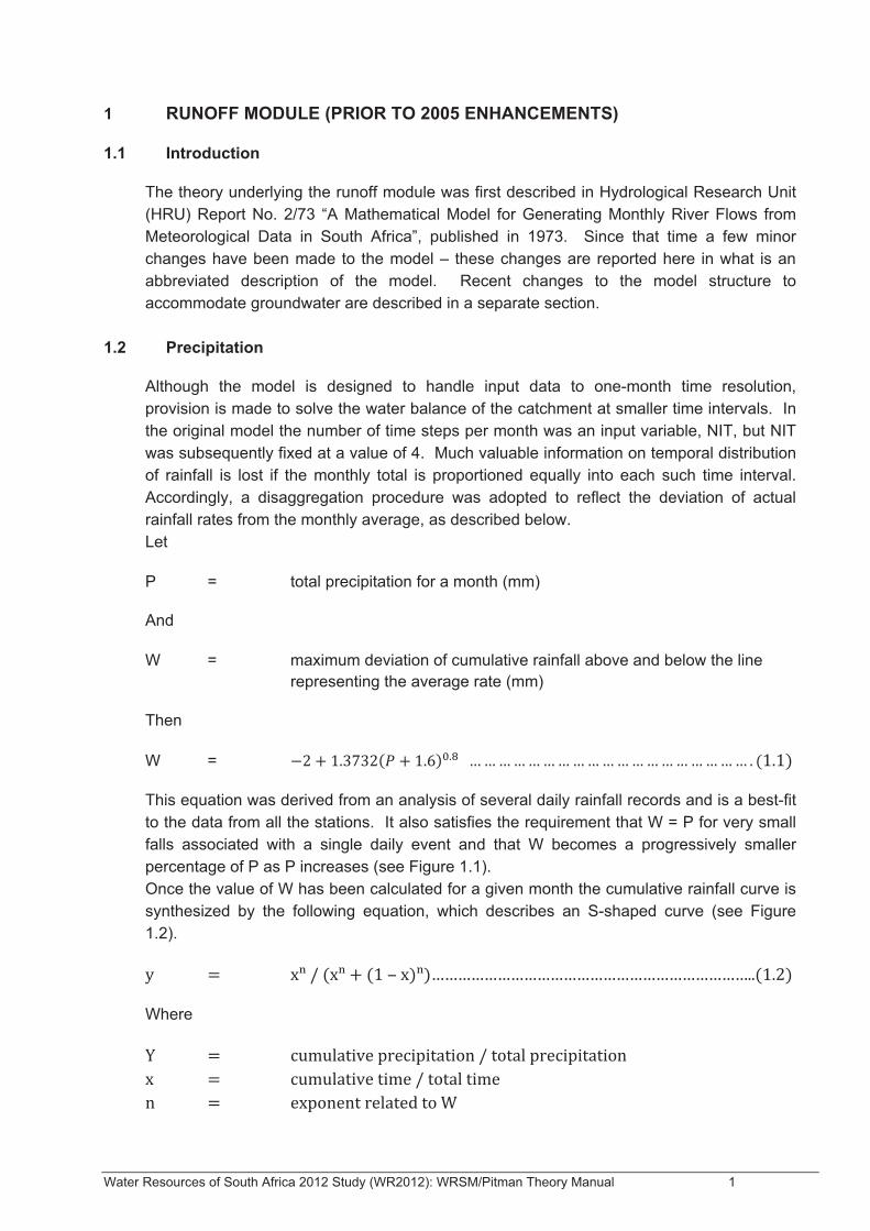
Although the model is designed to handle input data to one-month time resolution, provision is made to solve the water balance of the catchment at smaller time intervals. In the original model the number of time steps per month was an input variable, NIT, but NIT was subsequently fixed at a value of 4. Much valuable information on temporal distribution of rainfall is lost if the monthly total is proportioned equally into each such time interval. Accordingly, a disaggregation procedure was adopted to reflect the deviation of actual rainfall rates from the monthly average, as described below. Let
P = total precipitation for a month (mm)
And
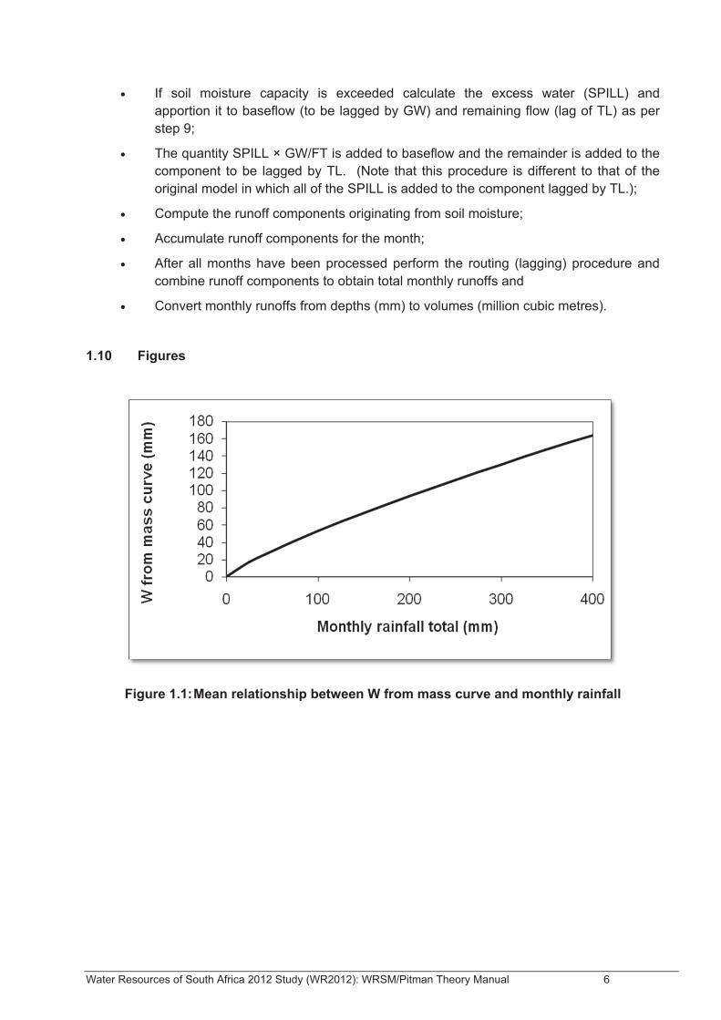
W = maximum deviation of cumulative rainfall above and below the line representing the average rate (mm)
Then
W =
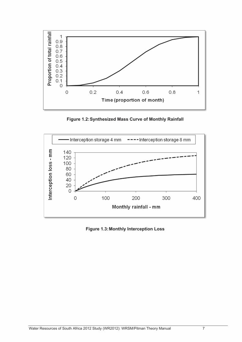
This equation was derived from an analysis of several daily rainfall records and is a best-fit to the data from all the stations. It also satisfies the requirement that W = P for very small falls associated with a single daily event and that W becomes a progressively smaller percentage of P as P increases (see Figure 1.1). Once the value of W has been calculated for a given month the cumulative rainfall curve is synthesized by the following equation, which describes an S-shaped curve (see Figure 1.2).
Where

Water Resources of South Africa 2012 Study (WR2012): WRSM/Pitman Theory Manual 2
The relationship between n and W within the range of likely values of P is given by the following equation:
1.3 Catchment rainfall
Catchment rainfall, which is a fundamental input to the runoff, irrigation, reservoir and channel modules, is derived by “averaging” the rainfall records of a number of individual stations. The method of averaging – as described below – is designed to avoid bias, especially when dealing with mountainous catchments where isohyetal gradients are steep. For each month for which catchment rainfall is required, let:
Pn = Monthly precipitation for rain gauge no. “n”. Mn = Mean annual precipitation (MAP) for rain gauge no. “n” N = Total no. of rain gauges used in the averaging process. PC = Catchment rainfall expressed as a percentage of its MAP PC = 100 [(Pn / Mn)] / N
The method gives equal weight to all stations used, but has the advantage that individual station records can vary, provided there is at least one record available at all times. The output, in the form of monthly rainfall percentals, is converted to millimetres in the model by application of the appropriate MAP.
1.4 Interception
To estimate the total interception losses over a month, the following assumptions were made:
• the total rainfall on any rain-day results from one event only and
• the water held in interception storage has time to evaporate completely between successive rain-days.
With these assumptions in mind it was possible to derive monthly interception losses for a number of daily rainfall records. The best-fit curves of interception loss versus monthly rainfall took the following form:
Where
For the range of interception storages to be applicable (0 – 10 mm), the empirical relationships between a, b and PI (interception storage) were found to be:
Water Resources of South Africa 2012 Study (WR2012): WRSM/Pitman Theory Manual 3
and
Figure 1.3 shows the relationship between interception loss and monthly rainfall for interception storages of 4 and 8 mm.
1.5 Surface runoff
Surface runoff is taken to be derived from two components, namely:
• runoff from impervious areas and
• runoff resulting from rainfall not absorbed by the soil.
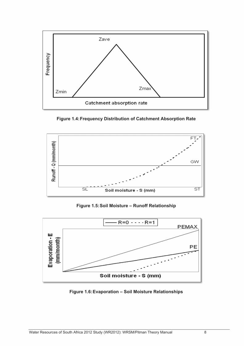
The first component is easily computed by multiplying catchment rainfall by the area of catchment that is impervious. In the original model the impervious fraction (AI) was fixed, but this has been amended so that a time-varying AI can be entered to reflect the growth of urbanized areas. In computing runoff from the second component it is assumed that absorption or infiltration varies across the catchment from a minimum rate to a maximum rate, with a symmetrical, triangular frequency distribution across the catchment (see Figure 1.4). The only variables needed to describe such a distribution of absorption rate are as follows:
Derivation of the equations for surface runoff is given in the original HRU Report No. 2/73; only the final equations are presented here. Let
and
Case 1:
Case 2:
Water Resources of South Africa 2012 Study (WR2012): WRSM/Pitman Theory Manual 4
Case 3:
Case 4:
1.6 Sub-surface runoff
Sub-surface runoff (Q in mm) is directly related to soil moisture according to the following equation, which is shown in graphical form in Figure 1.5:
Where
An additional parameter GW (maximum baseflow rate) is necessary in cases where the time lags of the different runoff components vary significantly. If the soil moisture is such that Q is less than GW the associated runoff is considered to be all baseflow and is lagged accordingly. If the storage is such that Q is greater than GW the remainder (Q – GW) is lagged to a much smaller degree than the baseflow component. A description of the lagging procedure follows.
1.7 Time delay of runoff
Lagging of runoff to the catchment outlet is achieved by application of the Muskingum equation with the weighting factor (x) set to zero for reservoir-type routing, as follows:
Where
and
In the context of this model the variables are given the following interpretation:
Water Resources of South Africa 2012 Study (WR2012): WRSM/Pitman Theory Manual 5
Subscripts and to I and O refer to the previous and current month’s runoffs respectively. In the model allowance is made to lag two components of runoff by assigning different ‘k’ values. All runoff from soil moisture that is equal to or less than GW is assigned a ‘k’ value equal to GL and all remaining runoff is assigned a somewhat shorter lag with
1.8 Evaporation from soil moisture
Catchment evapotranspiration, E, is assumed to be equal to potential evaporation, PE, when soil moisture, S, is at full capacity, ST. The relationship between E and S is assumed to be linear with a minimum S at which e is equal to zero. The slopes of the E S lines are assumed to lie between two limits, as defined by the variable ‘R’ that ranges between 0 and 1. When R = 0 the relationship E/PE = S/ST applies and when R = 1 the slopes of the E S lines are all the same and equal to PEMAX/ST, where PEMAX is the maximum monthly potential evaporation (see Figure 1.6). Derivation of the E S equation is given in HRU Report No. 2/73 – only the final equation is presented here.
Where
and
1.9 Calculation procedure
The calculation procedure for each month follows the following steps:
• Compute runoff from impervious area;
• Determine interception loss;
• Synthesize mass curve of rainfall for the month and calculate rainfall for each time step;
• The following 9 steps are performed for each time step;
• Subtract interception loss from rainfall;
• Compute surface runoff;
• Perform mass balance of soil moisture to determine soil moisture at end of time interval. Note that evaporation from soil moisture is adjusted to account for the evaporative loss from intercepted rainfall;
Water Resources of South Africa 2012 Study (WR2012): WRSM/Pitman Theory Manual 6
• If soil moisture capacity is exceeded calculate the excess water (SPILL) and apportion it to baseflow (to be lagged by GW) and remaining flow (lag of TL) as per step 9;
• The quantity SPILL × GW/FT is added to baseflow and the remainder is added to the component to be lagged by TL. (Note that this procedure is different to that of the original model in which all of the SPILL is added to the component lagged by TL.);
• Compute the runoff components originating from soil moisture;
• Accumulate runoff components for the month;
• After all months have been processed perform the routing (lagging) procedure and combine runoff components to obtain total monthly runoffs and
• Convert monthly runoffs from depths (mm) to volumes (million cubic metres).
1.10 Figures
Figure 1.1: Mean relationship between W from mass curve and monthly rainfall
Water Resources of South Africa 2012 Study (WR2012): WRSM/Pitman Theory Manual 7
Figure 1.2: Synthesized Mass Curve of Monthly Rainfall
Figure 1.3: Monthly Interception Loss
Water Resources of South Africa 2012 Study (WR2012): WRSM/Pitman Theory Manual 8
Figure 1.4: Frequency Distribution of Catchment Absorption Rate
Figure 1.5: Soil Moisture – Runoff Relationship
Figure 1.6: Evaporation – Soil Moisture Relationships

Water Resources of South Africa 2012 Study (WR2012): WRSM/Pitman Theory Manual 9
2 RESERVOIR MODULE (UNCHANGED FROM WR2005 TO WR2012 STUDIES)
2.1 Mass balance
The reservoir module performs a simple mass balance for each month, taking into account all inflows, outflows (including evaporation and spillage) and changes in storage state, as described below. All volumes are in million cubic metres and the reservoir surface area is in square km. Let
Subscripts and to variables S and A refer to the beginning and end of the month respectively. Net evaporation loss is calculated, based on the area at the start of the month, as follows:
The mass balance is first done assuming the dam neither dries up nor spills, as follows:
The preliminary month-end value of S is then compared with the capacity, CAP, to determine the spillage for the month, SPILL.
The next test is to check if the preliminary month-end value of S is less than zero, to determine whether the full draft D can be supplied, otherwise D is reduced as follows:
2.2 Area – storage relationship
The water balance keeps a continual track of the reservoir storage state S. The area for a given storage is calculated by the following equation:

Water Resources of South Africa 2012 Study (WR2012): WRSM/Pitman Theory Manual 10
The constant “b” is determined from the area-capacity tables of the reservoir to be modelled, however, if such information is unavailable a value of “b” equal to 0.6 is assumed. (A “b” of 0.6 represents the average for all reservoirs in South Africa.) The value of “a” is calculated by putting A = FSA and S = CAP into the above equation.
2.3 Controlled releases or draft – D
Controlled releases can be withdrawals from the reservoir or compensation releases downstream. There are three types of release/draft, namely:
• Supplies to an irrigation module, which are first calculated by that module;
• A time series of demands, covering the period to be simulated or
• A set of 12 demands, one for each calendar month, with the option of reducing demand when the storage state S falls below a prescribed level.
Option 3 requires a “trigger level” of storage, below which the demands are reduced, and a reduction factor that is applied to the demand. The calculation is set out below. Let
Then

Water Resources of South Africa 2012 Study (WR2012): WRSM/Pitman Theory Manual 11
3 IRRIGATION MODULE (PRIOR TO WR2005 STUDY ENHANCEMENTS)
The irrigation module is not meant to be used to design an irrigation layout but merely to estimate the effect of upstream irrigation usage on downstream river flow. The calculation of irrigation usage is based on the following variables:
The calculations proceed (for each month) as follows:
Volumetric demand (million cubic metres):
Return flow from the irrigation area (million cubic metres):
The calculations do not specifically allow for irrigation efficiency, as much of the “wasted” water will find its way back to the river. However, one can increase the total irrigation area to cater for inefficiencies – implying that water is wasted by “irrigating” areas outside those under crops.

Water Resources of South Africa 2012 Study (WR2012): WRSM/Pitman Theory Manual 12
4 IRRIGATION (WITH WR2005 STUDY ENHANCEMENTS) BY DR CE HEROLD
4.1 WQT Type 2 Algorithm
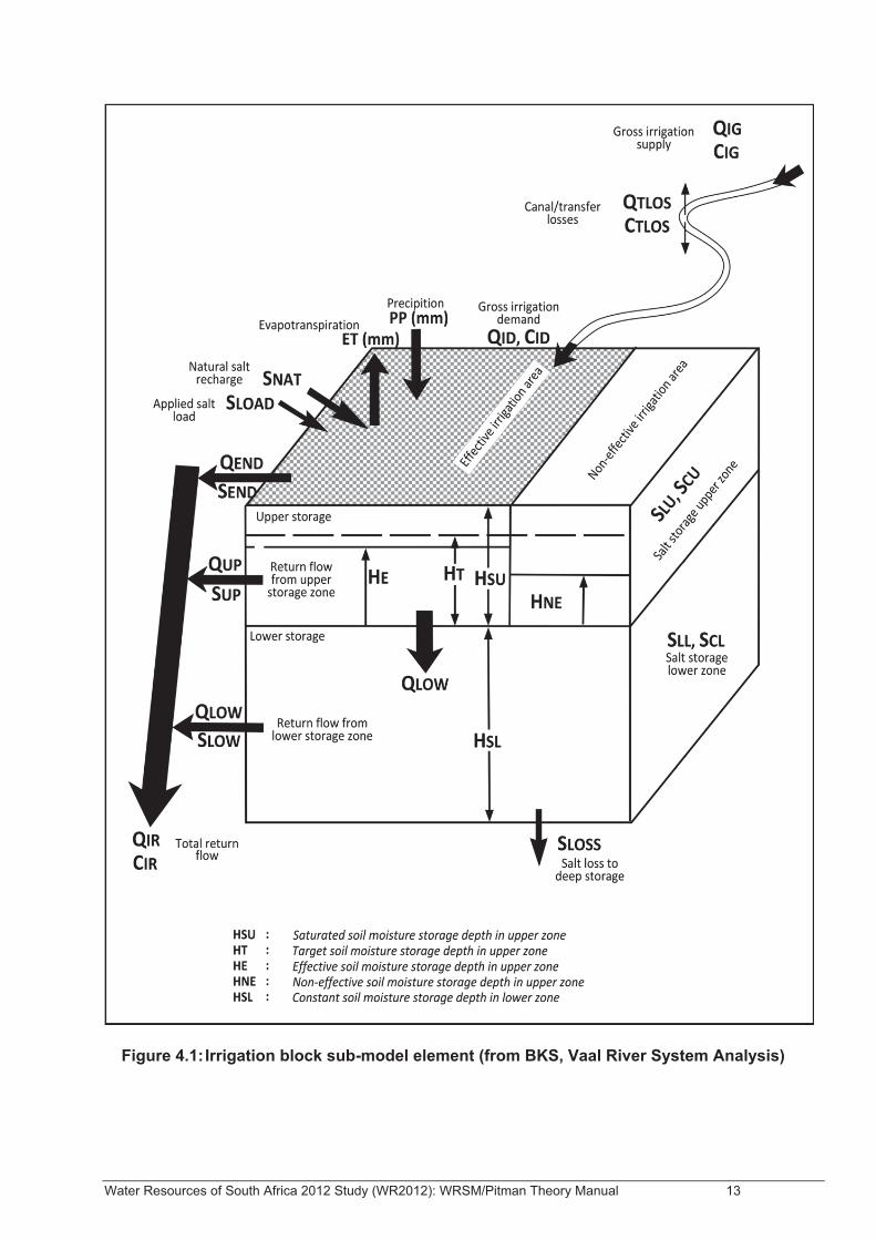
Irrigation Block Model An irrigation block sub-model has been developed which accounts for the continuity of mass for salt and allows further accumulation and flushing of salt from the irrigated lands. The irrigation sub-model structure is illustrated in Figure 4.1
4.1.1 Water Mass Balance The monthly unit irrigation demand (before allowances for losses) DIN (mm) is given as:
Where:
Water Resources of South Africa 2012 Study (WR2012): WRSM/Pitman Theory Manual 13
Figure 4.1: Irrigation block sub-model element (from BKS, Vaal River System Analysis)

Water Resources of South Africa 2012 Study (WR2012): WRSM/Pitman Theory Manual 14
The effective rainfall is calculated as follows:
Where
Allowing for the leaching requirements and application losses, the gross irrigation demand is given by:
Where:
An allowance is also made for canal/transfer losses in transporting from the raw water source to the irrigated land. Such losses are calculated as follows:
Or
Where:
Now if the gross irrigation supply requirement is greater than the available water from the raw water source, then the actual area irrigated during the month is given as follows:
Where:
Water Resources of South Africa 2012 Study (WR2012): WRSM/Pitman Theory Manual 15
Annual gross irrigation supply requirements are also compared with annual irrigation quotas to ensure that the water allocation limit is not violated. If the gross irrigation demand on an annual basis exceeds the annual allocation limit then the irrigated area is adjusted as follows:
Where:
The non-effective irrigation area is the proportion of the gross irrigation area not being irrigated and is given by:
Where:
At the beginning of each month the effective and non-effective irrigation areas are calculated. If the irrigation areas do change, the following calculations are performed to maintain the correct water balance.
Water Resources of South Africa 2012 Study (WR2012): WRSM/Pitman Theory Manual 16
The soil moisture storage depth is calculated on a monthly basis for both the effective irrigation area and the non-effective irrigation area. The calculation involves the monthly water balance of all water being applied and removed from the different areas. The water balance equation for the effective and non-effective irrigation area can be stated as follows (note that the water balance equation for the non-effective area is very similar with the irrigation demand omitted):
Where for the effective area:
Additional parameters used in equation
The return flow seepage from the effective irrigation area consists of two components, the natural runoff from the catchment as defined by the runoff from the pervious zone in the salt wash-off sub-model and the additional return flow seepage due to the soil moisture storage depth in the effective area of the upper zone. Return flow seepage from the effective area can be calculated as follows:
Where:
Water Resources of South Africa 2012 Study (WR2012): WRSM/Pitman Theory Manual 17
The return flow seepage from the non-effective area is given by the following equation:
Where:
The evapotranspiration losses from the irrigation area are very difficult to ascertain, but the following relationships are deemed appropriate for our purposes. For the evapotranspiration losses in the effective irrigation area, if the average solid moisture storage depth is less than the target soil moisture depth the following equation holds:
Where:
If the average soil moisture storage depth is greater than the target soil moisture storage depth, then two possibilities exist. If the potential lake evaporation, PEL is greater than the total crop water demands, the following equation holds:
If not then:
Where:
For the evapotranspiration losses in the non-effective irrigation area, the following equation holds:
Water Resources of South Africa 2012 Study (WR2012): WRSM/Pitman Theory Manual 18
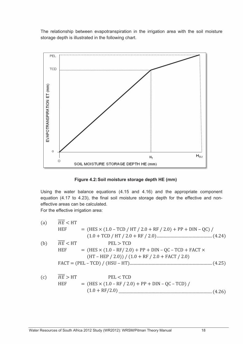
The relationship between evapotranspiration in the irrigation area with the soil moisture storage depth is illustrated in the following chart.
Figure 4.2: Soil moisture storage depth HE (mm) Using the water balance equations (4.15 and 4.16) and the appropriate component equation (4.17 to 4.23), the final soil moisture storage depth for the effective and non-effective areas can be calculated. For the effective irrigation area:
Water Resources of South Africa 2012 Study (WR2012): WRSM/Pitman Theory Manual 19
For the non-effective irrigation area
If the calculated final soil moisture storage depth is greater than the saturated soil moisture storage depth then the following adjustments are made:
The total return flow volume, RET (10 m³), from the irrigation sub-model is calculated as:
The total return flow from the irrigation sub-model is assumed to come from three different paths. (a) surface runoff directly from the area (b) runoff seepage directly from the upper zone (c) runoff seepage from the upper zone into the lower zone and then into the stream. The return flows from each path are calculated as follows:
Where:
4.2 Salt Mass Balance
The assumption is made in the irrigation block sub-model that complete mixing of salts through the entire scheduled area is achieved. Water losses en-route to the irrigated land via canals and farm dams are assumed to be partly due to evaporation (no salt lost) and partly due to seepage losses outside of the irrigation scheme. Hence, the irrigation salt load lost en-route is calculated as follows:
Water Resources of South Africa 2012 Study (WR2012): WRSM/Pitman Theory Manual 20
Where:
The sale load reaching the irrigation scheme is given by:
Where:
The net application of salt load to the irrigated area which accounts for fertilizers, gypsum and crop export is calculated as follows:
Where:
The additional salt load on the catchment due to natural salt recharge is given as follows:
Where:
The salt load leaving the various zones of the irrigated land is assumed to be proportionate to the respective TDS concentrations at the beginning of the month. Assume that the rejected water leaves at the TDS concentration of the applied irrigation water. Hence the salt load leaving the irrigated land by application rejection (surface runoff) can be calculated as follows:
Water Resources of South Africa 2012 Study (WR2012): WRSM/Pitman Theory Manual 21
The salt load for the return flow from the upper storage zone, SUP (tons) is given by the following equation:
Where:
The sale load for the return flow from the lower storage zone, SLOW (tons) is given by the following equation:
Where:
In addition to the salt load entering and leaving the irrigated land, allow for a slow bleed-off of salt into deeper, inaccessible storage below the irrigated land. The salt loss below can be evaluated as follows
Where:
The salt load passed from the upper storage zone to the lower storage zone is evaluated using QLOW, the return flow through the lower zone and a deep percolation salt concentration factor. This factor accounts for the salt load in the upper zone washing into the lower zone. This salt load is given by the following equation:
Where:
Water Resources of South Africa 2012 Study (WR2012): WRSM/Pitman Theory Manual 22
The salt balance continuity equation for the upper storage zone of the irrigation block sub-model is given by the following equation:
Where:
The salt balance continuity equation for the lower storage zone of the irrigation block sub-model is given by the following equation:
Where:
The total salt load leaving the irrigation block sub-model is given by the following equation:
Where:
After each year of irrigation application (the beginning of month 1), the gross irrigated area (scheduled irrigation area) can grow. To account for the additional salt load in the new irrigated area, a few assumptions are made. First, any additional irrigated land is taken from the pervious zone area of the related salt wash-off sub-model for the catchment. Therefore the pervious zone area is reduced by the amount the irrigated area is increased. The initial TDS concentrations of the new irrigated area is calculated such that the return flow seepage from the new portion of irrigated land is equal to the TDS concentration of the ground water storage in the salt wash-off sub-model of the associated catchment. This is calculated using the following equation.
Where:
It is also assumed that the surface salt storage for that portion of the pervious zone in the salt wash-off sub-model of this catchment brought under irrigation is added to the upper storage zone of the irrigation block.
Water Resources of South Africa 2012 Study (WR2012): WRSM/Pitman Theory Manual 23
Hence the total salt load gain to the upper zone if given as follows:
Where:
The total salt gain to the lower zone is given as follows:
Where:
For the salt wash-off sub-model the salt loss in the pervious zone, SLP (tons) is equal to:
and the salt loss in the groundwater zone, SLG (tons) is equal to :
It is likely that the salt load gain in the irrigation block sub-model (SGU + SGL) will be greater than the salt load loss in the salt wash-off sub-model (SLP + SLG). This can be rationalised as the irrigation sub-model activating a deeper salt storage which was not available to the salt wash-off sub-model, due to the raising of the local water table form irrigation application. If the gross irrigation supply requirements is met using flow from a dependent route, the salt load leaving the irrigation block sub-model using equations 4.1 to 4.49 can be expressed as:
Where:

Water Resources of South Africa 2012 Study (WR2012): WRSM/Pitman Theory Manual 24
Hence, the salt load leaving the irrigation block sub-model can be expressed in terms of a linear equation with one set of unknowns, the TDS concentration of the dependent route.
4.3 Irrigation Practice
The gross irrigation demand during the month must include an allowance for losses, which in turn is a function of the irrigation method employed, and for additional water for leaching salts out of the irrigated lands. The following are typical irrigation efficiencies for different irrigation practices (Loxton Venn, 1985):
• Flood irrigation : 65 %
• Sprinkler irrigation : 75 %
• Centre pivot irrigation : 85 %
• Drip irrigation : 85 %
The mix of irrigation practices in various regions in the Vaal system gives the following overall efficiencies:
• Barrage to Bloemhof (riparian) : 73%
• Christiana : 74 %
• Vaalharts/Taung : 67 %
• Barkly West : 73 %
• Douglas – Bucklands : 69 %
For most irrigation schemes the leaching factor (LF) is known, or can be estimated from a knowledge of the mix of crops, soil types, drainage conditions, irrigation practice and the general quality of the applied water. For the purposes of this model LF is assumed constant for any irrigation scheme, although it is in effect a function of the quality of the applied irrigation water. This simplifying assumption is justified by the consideration that few farmers measure the salinity conditions in the root zone of their lands on a regular basis, and fewer still adjust the leaching fraction in accordance with changes in the measure salinity.
4.4 Irrigation return flow
An additional parameter was added to the standard WQT irrigation return flow equation, namely the canal transfer loss. Some of the canal losses are lost from the system as result of evaporation and some can return to the natural or artificial draining systems through seepage as return flows.

Water Resources of South Africa 2012 Study (WR2012): WRSM/Pitman Theory Manual 25
Where:
The total return flow volume from the irrigation sub-model that is currently defined as:
Where:
Water Resources of South Africa 2012 Study (WR2012): WRSM/Pitman Theory Manual 26
5 WQT-SAPWAT METHOD IMPROVEMENTS
5.1 SAPWAT Representative Crop
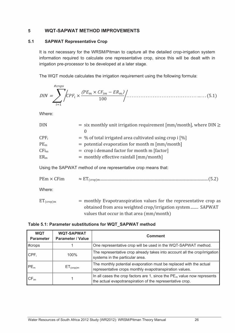
It is not necessary for the WRSM/Pitman to capture all the detailed crop-irrigation system information required to calculate one representative crop, since this will be dealt with in irrigation pre-processor to be developed at a later stage. The WQT module calculates the irrigation requirement using the following formula:
Where:
Using the SAPWAT method of one representative crop means that:
Where:
Table 5.1: Parameter substitutions for WQT_SAPWAT method
WQT Parameter
WQT-SAPWAT Parameter / Value Comment
#crops 1 One representative crop will be used in the WQT-SAPWAT method.
CPFi 100% The representative crop already takes into account all the crop/irrigation systems in the particular area.
PEm ET(crop)m The monthly potential evaporation must be replaced with the actual representative crops monthly evapotranspiration values.
CFim 1 In all cases the crop factors are 1, since the PEm value now represents the actual evapotranspiration of the representative crop.
Water Resources of South Africa 2012 Study (WR2012): WRSM/Pitman Theory Manual 27
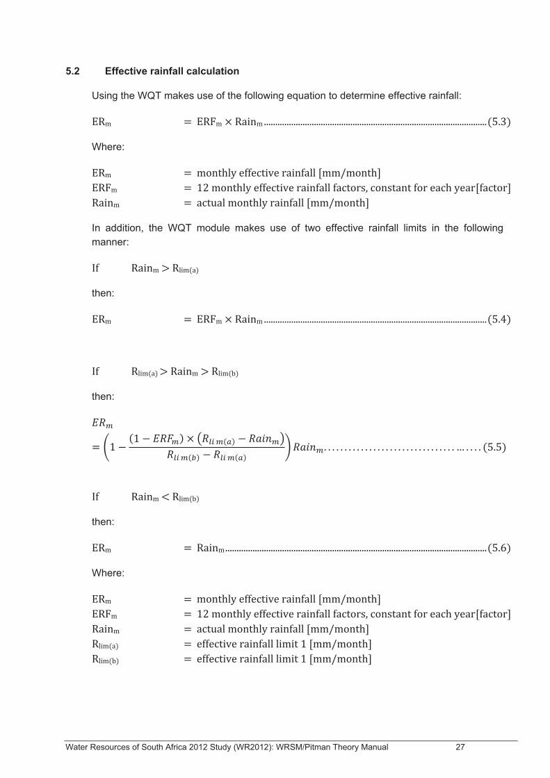
5.2 Effective rainfall calculation
Using the WQT makes use of the following equation to determine effective rainfall:
Where:
In addition, the WQT module makes use of two effective rainfall limits in the following manner:
then:
then:
then:
Where:
Water Resources of South Africa 2012 Study (WR2012): WRSM/Pitman Theory Manual 28
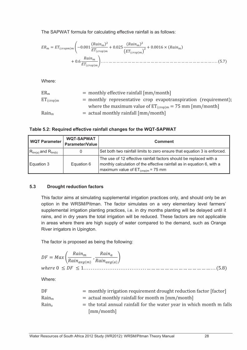
The SAPWAT formula for calculating effective rainfall is as follows:
Where:
Table 5.2: Required effective rainfall changes for the WQT-SAPWAT
WQT Parameter WQT-SAPWAT Parameter/Value Comment
Rlim(a) and Rlim(b) 0 Set both two rainfall limits to zero ensure that equation 3 is enforced.
Equation 3 Equation 6 The use of 12 effective rainfall factors should be replaced with a monthly calculation of the effective rainfall as in equation 6, with a maximum value of ET(crop)m = 75 mm
5.3 Drought reduction factors
This factor aims at simulating supplemental irrigation practices only, and should only be an option in the WRSM/Pitman. The factor simulates on a very elementary level farmers’ supplemental irrigation planting practices, i.e. in dry months planting will be delayed until it rains, and in dry years the total irrigation will be reduced. These factors are not applicable in areas where there are high supply of water compared to the demand, such as Orange River irrigators in Upington. The factor is proposed as being the following:
Where:
Water Resources of South Africa 2012 Study (WR2012): WRSM/Pitman Theory Manual 29
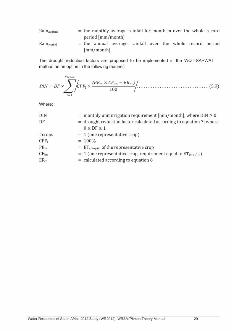
The drought reduction factors are proposed to be implemented in the WQT-SAPWAT method as an option in the following manner:
Where:
Water Resources of South Africa 2012 Study (WR2012): WRSM/Pitman Theory Manual 30
6 IRRIGATION: WQT TYPE 4 METHODOLOGY (WR2012 STUDY) BY DR CE HEROLD
6.1 Introduction
The irrigation sub-module as used in the following models has been enhanced to account for several deficiencies in the previous versions of the sub-module:
• WQT Salt Washoff Model; • The Water Resources Yield Model (WRYM) and • The Water Resources Planning Model (WRPM).
The issues related with the previous versions of the sub-module were identified during the Berg River Water Availability Assessment Study. The return flow generated by the systems models for Western Cape climatic conditions was unrealistically high, due to most of the rain falling in the lowest evaporation period. The result was that the irrigation return flow calculation could not be used in this (and future) studies for this region which necessitated the use of time consuming alternative methods.
6.2 Improvements to the return flow calculation and effects on salt balances
The main concern identified was the way in which return flow is calculated in the water resources systems models. The return flow generated in the irrigation sub-module is based on the sub-surface soil moisture balance calculations. The soil moisture balance calculation did not yield realistic results in areas where most of the rainfall occurred in the period when the least evaporation occurred. A method of dealing with this problem was formulated and involved making changes to the two sub-surface soil moisture stores in the model. Additionally the functionality of accounting for canal losses that adds to return flow was implemented to also include the effect on salt balances. The algorithms used to simulate deep groundwater losses were also improved.
6.3 Irrigation demand calculations
Minor functionality improvements to the irrigation demand calculations in the water resources systems models were also made. These improvements are partly due to the changes being made to the return flow calculations and the salt balances, and partly to improve the WQT to have the same functionality that already exist in the WRSM/Pitman, WRYM and the WRPM. These changes include:
• Improved annual allocation limit calculations; • Effects of drought requirement reduction on salt balances; • Physical supply constraints functionality and • FAO effective rainfall calculation.
Water Resources of South Africa 2012 Study (WR2012): WRSM/Pitman Theory Manual 31
6.4 Model Initialisation
6.4.1 Input Data Description The input data description for the WQT model is provided in Appendix A of this document. The WRPM and WRYM input data formats are provided in the WRYM and WRPM Input Data and File Formats Documents for Version 4.4, dated 28 February 2013.
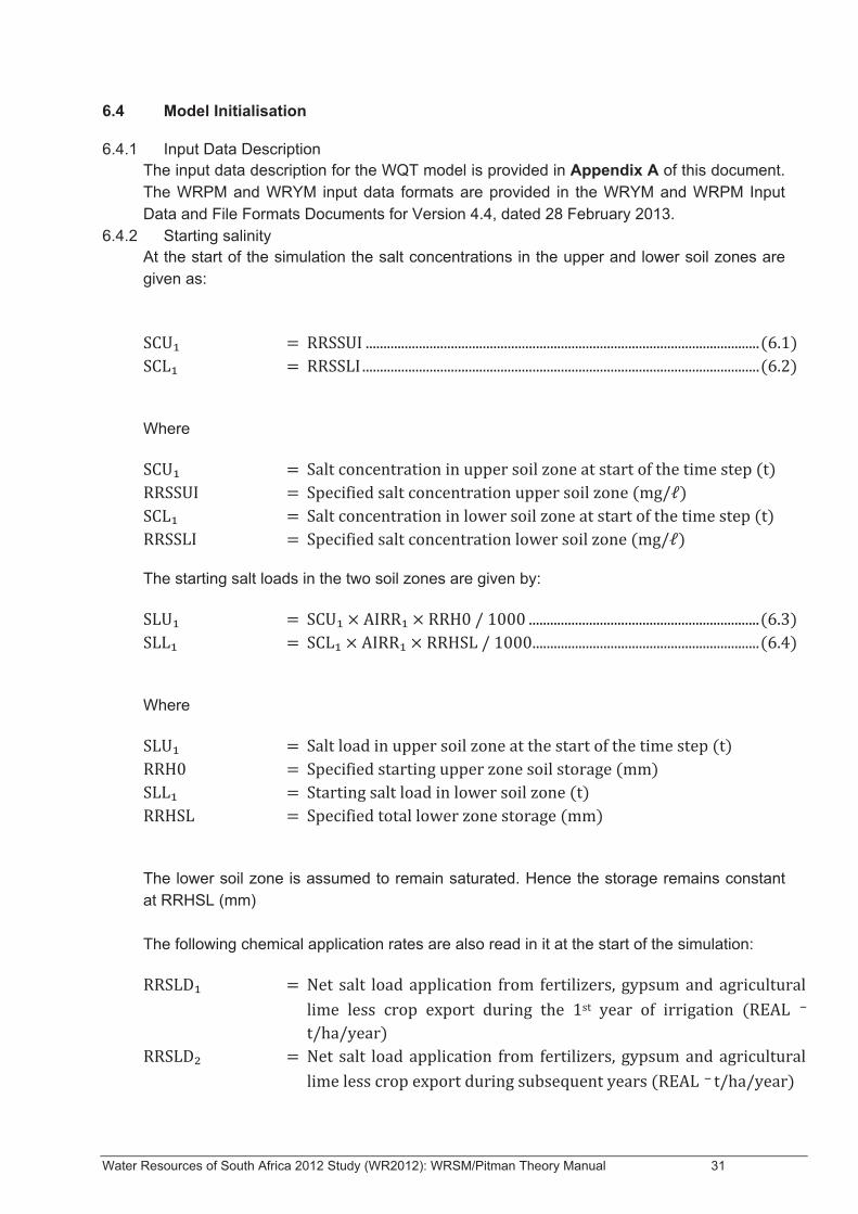
6.4.2 Starting salinity At the start of the simulation the salt concentrations in the upper and lower soil zones are given as:
Where
The starting salt loads in the two soil zones are given by:
Where
The lower soil zone is assumed to remain saturated. Hence the storage remains constant at RRHSL (mm) The following chemical application rates are also read in it at the start of the simulation:
Water Resources of South Africa 2012 Study (WR2012): WRSM/Pitman Theory Manual 32
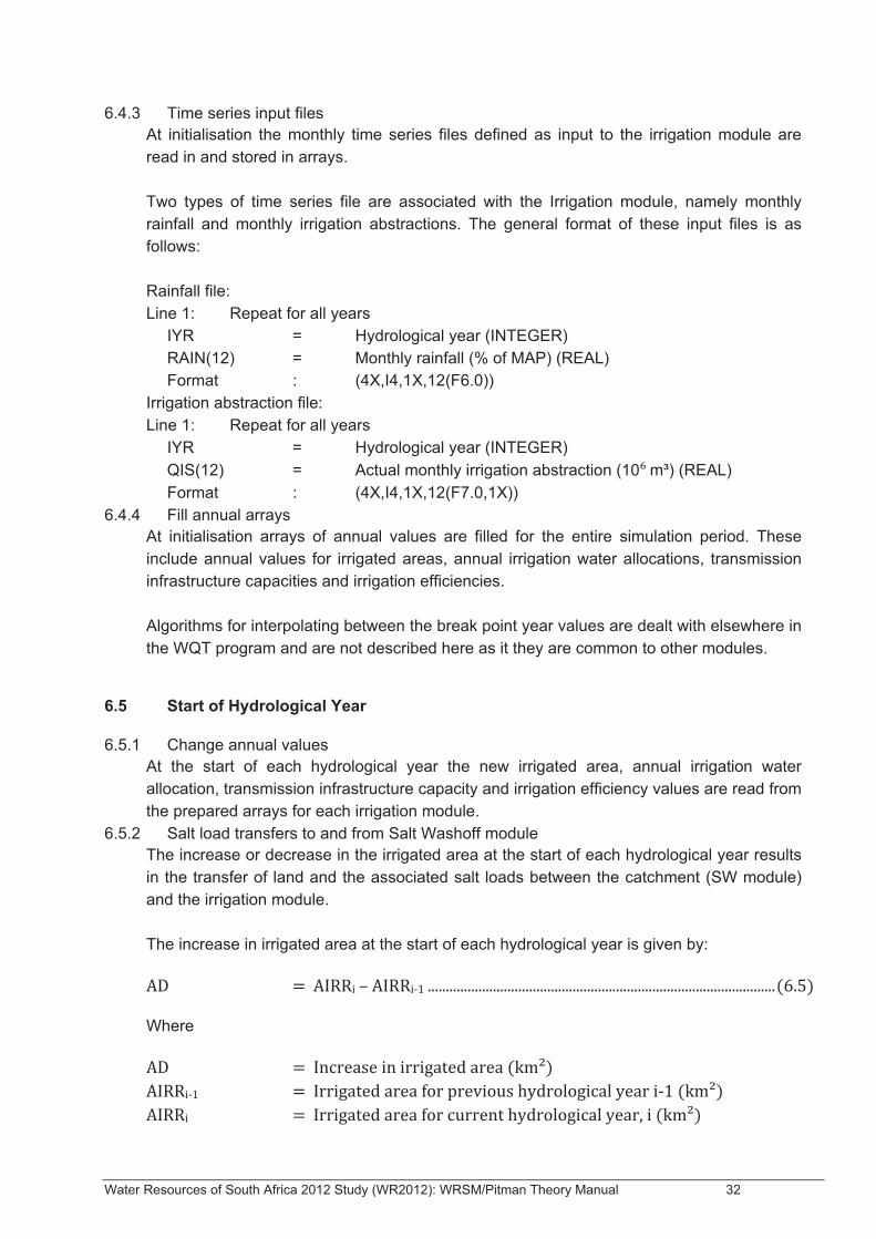
6.4.3 Time series input files At initialisation the monthly time series files defined as input to the irrigation module are read in and stored in arrays. Two types of time series file are associated with the Irrigation module, namely monthly rainfall and monthly irrigation abstractions. The general format of these input files is as follows: Rainfall file: Line 1: Repeat for all years IYR = Hydrological year (INTEGER) RAIN(12) = Monthly rainfall (% of MAP) (REAL) Format : (4X,I4,1X,12(F6.0)) Irrigation abstraction file: Line 1: Repeat for all years IYR = Hydrological year (INTEGER) QIS(12) = Actual monthly irrigation abstraction (10 m³) (REAL) Format : (4X,I4,1X,12(F7.0,1X))
6.4.4 Fill annual arrays At initialisation arrays of annual values are filled for the entire simulation period. These include annual values for irrigated areas, annual irrigation water allocations, transmission infrastructure capacities and irrigation efficiencies. Algorithms for interpolating between the break point year values are dealt with elsewhere in the WQT program and are not described here as it they are common to other modules.
6.5 Start of Hydrological Year
6.5.1 Change annual values At the start of each hydrological year the new irrigated area, annual irrigation water allocation, transmission infrastructure capacity and irrigation efficiency values are read from the prepared arrays for each irrigation module.
6.5.2 Salt load transfers to and from Salt Washoff module The increase or decrease in the irrigated area at the start of each hydrological year results in the transfer of land and the associated salt loads between the catchment (SW module) and the irrigation module. The increase in irrigated area at the start of each hydrological year is given by:
Where
Water Resources of South Africa 2012 Study (WR2012): WRSM/Pitman Theory Manual 33
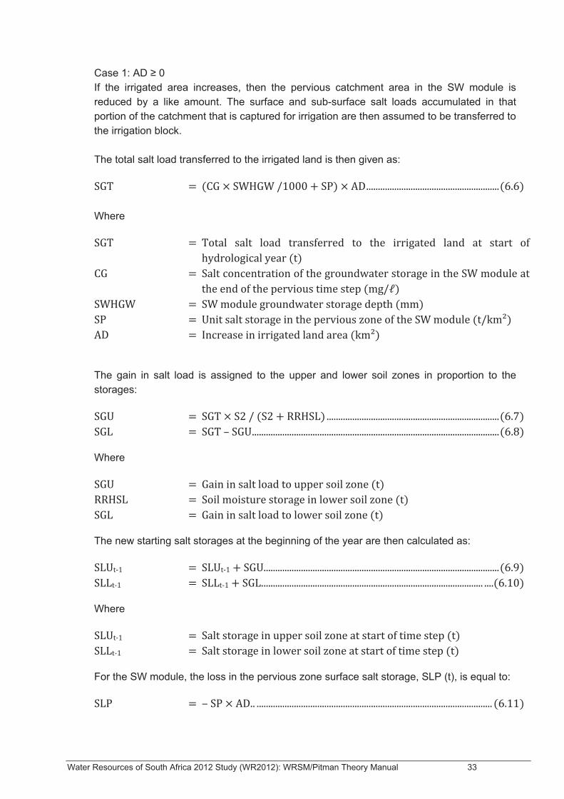
Case 1: AD 0 If the irrigated area increases, then the pervious catchment area in the SW module is reduced by a like amount. The surface and sub-surface salt loads accumulated in that portion of the catchment that is captured for irrigation are then assumed to be transferred to the irrigation block. The total salt load transferred to the irrigated land is then given as:
Where
The gain in salt load is assigned to the upper and lower soil zones in proportion to the storages:
Where
The new starting salt storages at the beginning of the year are then calculated as:
Where
For the SW module, the loss in the pervious zone surface salt storage, SLP (t), is equal to:
Water Resources of South Africa 2012 Study (WR2012): WRSM/Pitman Theory Manual 34
The salt loss from the groundwater storage of the SW module, SLG (t), is given by:
Case 2: AD < 0 If the irrigated area decreases, then the corresponding portion of the salt load must be transferred to the SW module. The reductions in the salt load stored in the upper and lower soil zones are calculated as:
There is insufficient information to assign a proportion of the transferred salt load to the pervious catchment surface store in the SW module. Instead the entire load is transferred to the subsurface salt storage. This approximation implies that the previous irrigation will have depleted the amount of salt stored at the surface and available for washoff. The effect of the approximation is further diminished provided the irrigated area is small compared to the total catchment area and the fact that irrigated areas seldom decline. The increases in the salt storages in the SW module are therefore:
6.6 Monthly Loop
6.6.1 Irrigation water demand Net unit demand Two options are allowed in the new model to calculate the effective rainfall:
• The modified WQT method and
• The SAPWAT method.
Modified WQT method Calculation of the monthly unit irrigation demand is based on the algorithms used in the original WQT model (Allen and Herold, 1988). The monthly unit irrigation demand before allowances for losses, DIN (mm) is calculated as:
Water Resources of South Africa 2012 Study (WR2012): WRSM/Pitman Theory Manual 35
Where
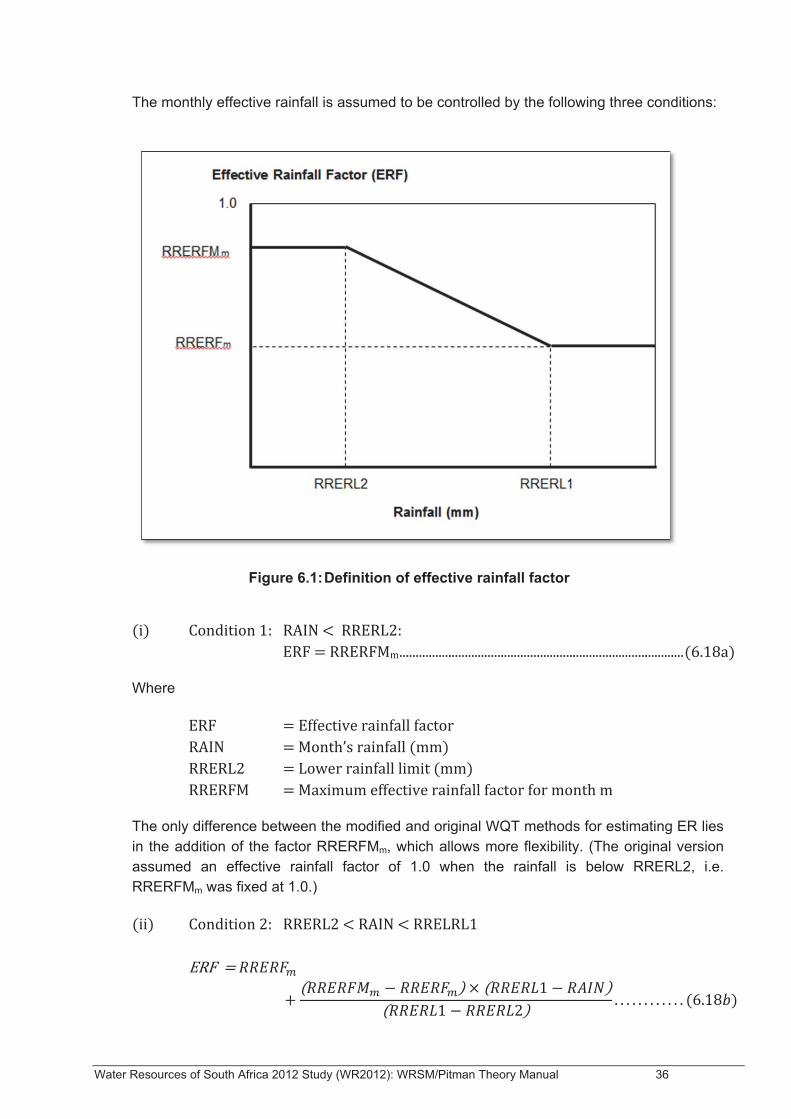
If DIN is less than zero, then DIN is set to zero. The effective rainfall, ER, is used in place of the actual month’s rainfall to allow for the fact that there is a time lag (often several hours) between the call for irrigation water and the arrival of the scheduled water at field edge, due to transmission through the canal system. Administrative factors add to this delay. If it rains in the meantime, then part of the irrigation water will be wasted. High rainfall events can also exceed the infiltration rate of the soil, resulting in surface runoff thereby making part of the rainfall inaccessible to the crop. It must also be observed that the rainfall distribution during a month (the computational time step) is not uniform. Thus for part of the month (usually a short part) the rainfall may exceed the crop demand, while for the rest of the month there may be no rainfall at all, necessitating more irrigation application than might have been surmised had the month’s rainfall been uniform. This temporal variation means that the effective rainfall factor will almost invariably be smaller than the rainfall factor based on daily rainfall data. This distinction is extremely important when choosing effective rainfall factors. At the other end of the scale, for low rainfall, it is generally assumed that nearly all of the rainfall is effective since none of the rainfall will be spilled or exceed the infiltration rate of the soil. However, it could be argued that under such conditions the rainfall may be too low for the farmer or dam operators to take into account when scheduling releases. Or some of the rainfall may be lost to canopy interception without reaching the ground. For this reason the modified WQT version allows the user to specify an upper limit to the effective rainfall factor. The effective rainfall factor, ERF, is defined as a function of the month’s rainfall. This relationship is illustrated in Figure 6.1. This factor is multiplied by the month’s rainfall to obtain the effective rainfall (ER).
Water Resources of South Africa 2012 Study (WR2012): WRSM/Pitman Theory Manual 36
The monthly effective rainfall is assumed to be controlled by the following three conditions:
Figure 6.1: Definition of effective rainfall factor
Where
The only difference between the modified and original WQT methods for estimating ER lies in the addition of the factor RRERFMm, which allows more flexibility. (The original version assumed an effective rainfall factor of 1.0 when the rainfall is below RRERL2, i.e. RRERFMm was fixed at 1.0.)
Water Resources of South Africa 2012 Study (WR2012): WRSM/Pitman Theory Manual 37
Where
The following limits apply:
And
The effective rainfall is then given by:
SAPWAT method The SAPWAT method follows similar calculation techniques for the net unit irrigation demand, but has been pre-applied to each quaternary catchment taking account of the areas of land under different crops. The results have been aggregated to form an effective single crop for the quaternary. Hence equation (6.17a) simplifies to:
Where
The SAPWAT method calculates the effective rainfall for the month as:
6.6.2 Field edge irrigation demand The monthly field edge irrigation demand needs to account for the area irrigated and the irrigation efficiency.
Water Resources of South Africa 2012 Study (WR2012): WRSM/Pitman Theory Manual 38
Where
The user provides irrigated areas for each specified break point year. Either linear or exponential interpolation can be used to calculate the areas, AIRRi, for each intermediate year, i. An upper limit on the allowable irrigated area is: 0 AIRRi (SWA – SWUA), where SWA (km²) is the total catchment area and SWUA (km²) is the urbanised area. The irrigation efficiency factor accounts for different irrigation practices not applying the water uniformly over the irrigated land, resulting in wastage. Flood irrigation has the lowest efficiency, drip irrigation the highest. Typical irrigation efficiency factors are as follows (Loxton Venn, 1985):
• Flood irrigation : 65%
• Sprinkler irrigation : 75%
• Centre pivot irrigation : 85%
• Drip irrigation : 85%
One difficulty associated with the irrigation efficiency is the fate of the “inefficient” proportion of the water applied. DIN purports to account for the water balance of the soil since it is assumed to maintain the soil moisture at an optimum level. It follows that any additional water applied to the land must either give rise to additional return flow or result in additional evapotranspiration loss. Loxton Venn (1985) estimated the irrigation efficiency at the Vaalharts irrigation scheme as 67%. This implies an additional 33% application to the irrigated lands. However, hydrological analyses of the Harts River carried out by Pitman (1987) for a similar period showed an annual return flow of 30 m³ × 10 , which was only 10% of the water supply to Vaalharts. This implies that supply inefficiency must have resulted in additional evapotranspiration losses of 23% (although some of this may have been lost to deep seated groundwater in this semi-arid region).
6.6.3 Drought reduction factor An option is provided to use a drought reduction factor, if applicable. This factor is as provided in the WRSM/Pitman model and is aimed at simulating supplemental irrigation practices only. The factor simulates on a very elementary level farmers’ supplemental irrigation planting practices. I.e. in dry months planting will be delayed until it rains, and in dry years the total irrigation will be reduced. This factor is not applicable in areas where the
Water Resources of South Africa 2012 Study (WR2012): WRSM/Pitman Theory Manual 39
water availability is large compared to the demand, such as Orange River irrigators in Upington. This factor is calculated as:
Where
A weakness of Equation (6.21a) is that it supposes prior knowledge of the year’s rainfall, RAINa. While this can be calculated by the model, in reality no farmer will know in advance what total rainfall will occur during the year. It is clear that the use of the drought reduction factor is at best an approximation. For all other cases DF is deactivated as follows:
The adjusted net unit irrigation demand, DIN1 (mm) is then calculated as:
6.6.4 Irrigation demand at supply source Allowance has to be made for transmission losses through the conveyance system to arrive at the gross water demand at the point of abstraction from the water source.
Where
Water Resources of South Africa 2012 Study (WR2012): WRSM/Pitman Theory Manual 40
6.6.5 Water allocation constraints Equation (6.23) represents the irrigation demand at the supply source. However, this full demand may not be met for the following reasons:
• Conveyance system and/or on farm system constraints
• Permissible allocation limit exceeded
• Insufficient water at source.
System capacity constraints The month’s water supply cannot exceed the capacity of the canal or pipeline supplying the irrigated land, or of the on-farm irrigation system. In effect there is no need to differentiate between the two types of constraint seeing as the WQT model simulates an entire irrigation module, in which the ruling constraint is all that matters. Hence the following checks have been included:
where RRCAPi is the limiting capacity of the system for year i (10 m³ /month) Provision is made to specify the capacities at breakpoint years and the method of interpolation to be used between specified breakpoints (linear or power). Permissible annual allocation limit exceeded The original WQT irrigation module allows for a specified maximum annual water allocation, RRMAi (10 m³). This is sound in principle, but was applied too simplistically, since it allowed full satisfaction of the monthly water demand until such time as the annual allocation was exceeded, after which irrigation ceased for the remainder of the hydrological year. The following procedure is intended to yield a more realistic distribution of the annual water allocation to the months of the year. Since the actual monthly rainfall for the remaining months of the year is never known in advance, it is necessary to devise a distribution based on mean monthly rainfall data and adjust the allocation available as the year progresses. The monthly distribution factors are pre-calculated as:
Where
Water Resources of South Africa 2012 Study (WR2012): WRSM/Pitman Theory Manual 41
For the modified WQT method, DINMm is pre-calculated from Equations (6.17a), (6.18a), (6.18b), (6.18c) and (6.19a), except that the variable RAIN (the actual month’s rainfall) is substituted with RAINMm (the mean rainfall for month m). RAINMm is calculated as:
Where
For the SAPWAT method, DINMm is pre-calculated from Equations (6.17b) and (6.19b), with the variable RAIN replaced by RAINMm. The original WQT irrigation module used growth factors that were multiplied by a single defined allocation (parameter RRMA) for GROWTH = 1.0. In the modified version the growth factor is dropped and instead the user directly species the actual allocation amounts for each breakpoint year, RRMAi (10 m³). Linear or power regressions are chosen for interpolation between the breakpoints. The nominal water allocation for each month is then calculated as:
Where
For the first month of the hydrological year the month’s allocation is fixed by Equation (6.27), but thereafter the unused portion of the allocation for previous months that have already passed is accumulated: At the start of every hydrological year the accumulated surplus, ACCALOC, is set to zero:
Where
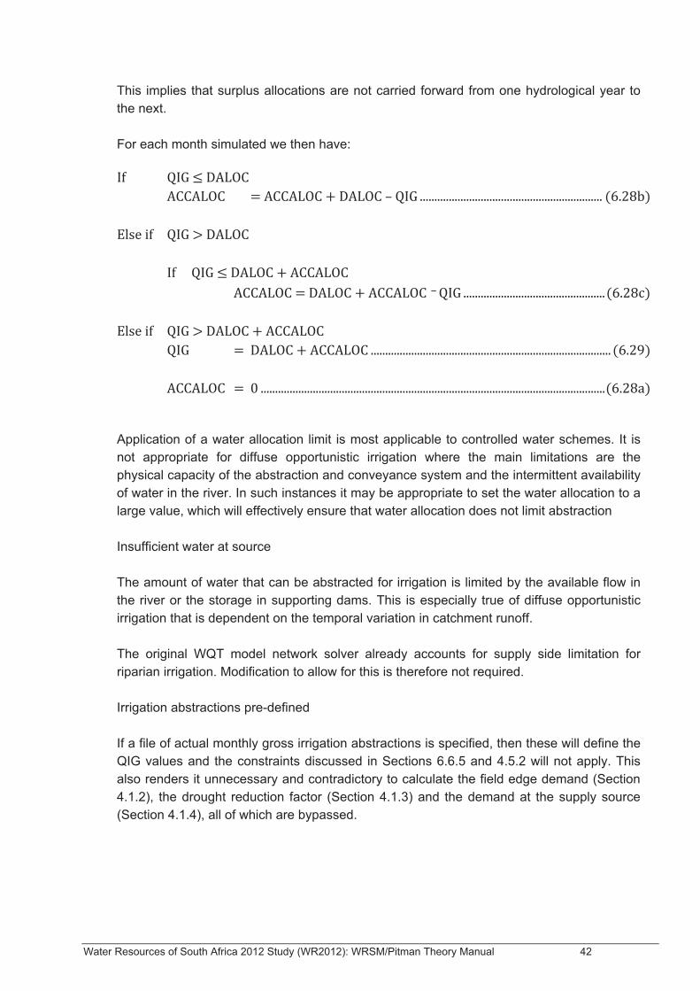
Water Resources of South Africa 2012 Study (WR2012): WRSM/Pitman Theory Manual 42
This implies that surplus allocations are not carried forward from one hydrological year to the next. For each month simulated we then have:
Application of a water allocation limit is most applicable to controlled water schemes. It is not appropriate for diffuse opportunistic irrigation where the main limitations are the physical capacity of the abstraction and conveyance system and the intermittent availability of water in the river. In such instances it may be appropriate to set the water allocation to a large value, which will effectively ensure that water allocation does not limit abstraction Insufficient water at source The amount of water that can be abstracted for irrigation is limited by the available flow in the river or the storage in supporting dams. This is especially true of diffuse opportunistic irrigation that is dependent on the temporal variation in catchment runoff. The original WQT model network solver already accounts for supply side limitation for riparian irrigation. Modification to allow for this is therefore not required. Irrigation abstractions pre-defined If a file of actual monthly gross irrigation abstractions is specified, then these will define the QIG values and the constraints discussed in Sections 6.6.5 and 4.5.2 will not apply. This also renders it unnecessary and contradictory to calculate the field edge demand (Section 4.1.2), the drought reduction factor (Section 4.1.3) and the demand at the supply source (Section 4.1.4), all of which are bypassed.
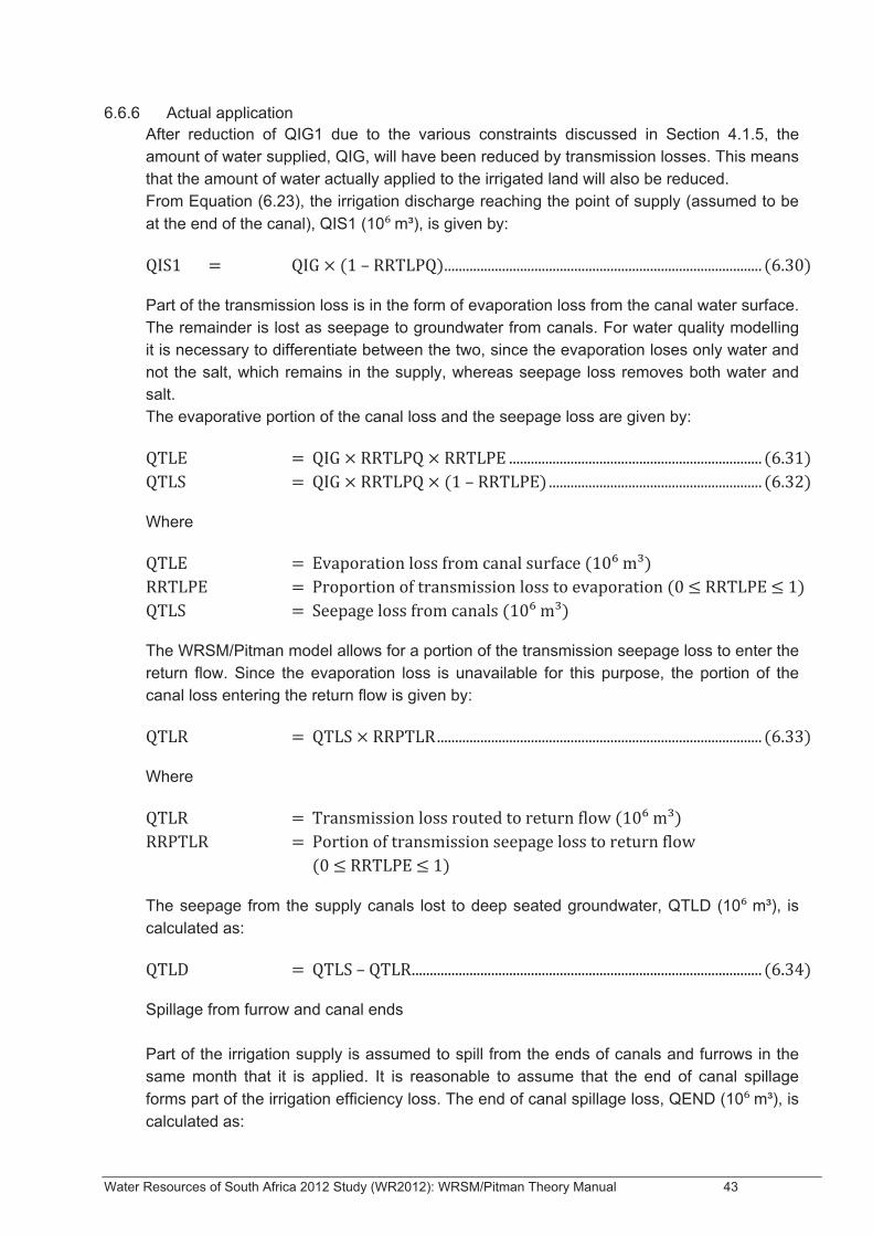
Water Resources of South Africa 2012 Study (WR2012): WRSM/Pitman Theory Manual 43
6.6.6 Actual application After reduction of QIG1 due to the various constraints discussed in Section 4.1.5, the amount of water supplied, QIG, will have been reduced by transmission losses. This means that the amount of water actually applied to the irrigated land will also be reduced. From Equation (6.23), the irrigation discharge reaching the point of supply (assumed to be at the end of the canal), QIS1 (10 m³), is given by:
Part of the transmission loss is in the form of evaporation loss from the canal water surface. The remainder is lost as seepage to groundwater from canals. For water quality modelling it is necessary to differentiate between the two, since the evaporation loses only water and not the salt, which remains in the supply, whereas seepage loss removes both water and salt. The evaporative portion of the canal loss and the seepage loss are given by:
Where
The WRSM/Pitman model allows for a portion of the transmission seepage loss to enter the return flow. Since the evaporation loss is unavailable for this purpose, the portion of the canal loss entering the return flow is given by:
Where
The seepage from the supply canals lost to deep seated groundwater, QTLD (10 m³), is calculated as:
Spillage from furrow and canal ends Part of the irrigation supply is assumed to spill from the ends of canals and furrows in the same month that it is applied. It is reasonable to assume that the end of canal spillage forms part of the irrigation efficiency loss. The end of canal spillage loss, QEND (10 m³), is calculated as:
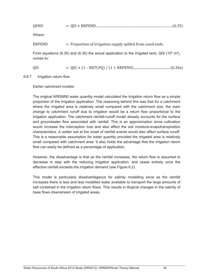
Water Resources of South Africa 2012 Study (WR2012): WRSM/Pitman Theory Manual 44
Where:
From equations (6.30) and (6.35) the actual application to the irrigated land, QIS (10 m³), comes to:
6.6.7 Irrigation return flow Earlier catchment models The original WRSM90 water quantity model calculated the irrigation return flow as a simple proportion of the irrigation application. The reasoning behind this was that for a catchment where the irrigated area is relatively small compared with the catchment size, the main change to catchment runoff due to irrigation would be a return flow proportional to the irrigation application. The catchment rainfall-runoff model already accounts for the surface and groundwater flow associated with rainfall. This is an approximation since cultivation would increase the interception loss and also affect the soil moisture-evapotranspiration characteristics. A wetter soil at the onset of rainfall events would also affect surface runoff. This is a reasonable assumption for water quantity provided the irrigated area is relatively small compared with catchment area. It also holds the advantage that the irrigation return flow can easily be defined as a percentage of application. However, the disadvantage is that as the rainfall increases, the return flow is assumed to decrease in step with the reducing irrigation application, and cease entirely once the effective rainfall exceeds the irrigation demand (see Figure 6.2). This model is particularly disadvantageous for salinity modelling since as the rainfall increases there is less and less modelled water available to transport the large amounts of salt contained in the irrigation return flows. This results in illogical changes in the salinity of base flows downstream of irrigated areas.
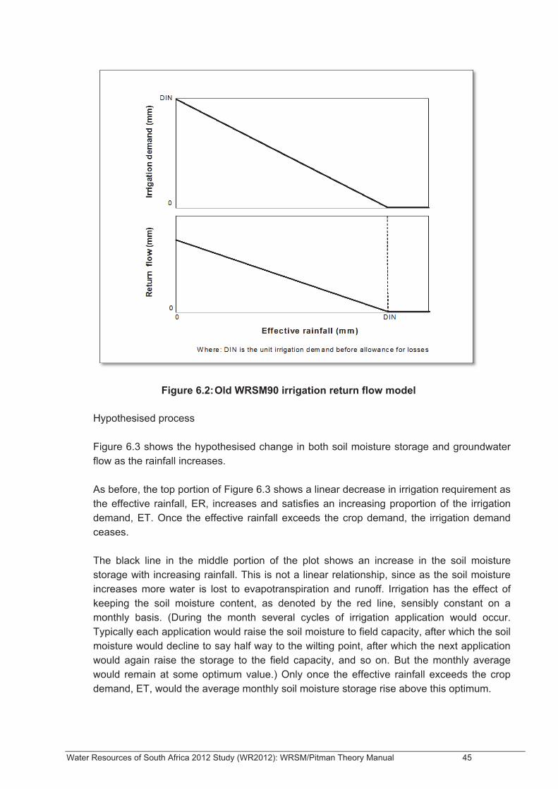
Water Resources of South Africa 2012 Study (WR2012): WRSM/Pitman Theory Manual 45
Figure 6.2: Old WRSM90 irrigation return flow model Hypothesised process Figure 6.3 shows the hypothesised change in both soil moisture storage and groundwater flow as the rainfall increases. As before, the top portion of Figure 6.3 shows a linear decrease in irrigation requirement as the effective rainfall, ER, increases and satisfies an increasing proportion of the irrigation demand, ET. Once the effective rainfall exceeds the crop demand, the irrigation demand ceases. The black line in the middle portion of the plot shows an increase in the soil moisture storage with increasing rainfall. This is not a linear relationship, since as the soil moisture increases more water is lost to evapotranspiration and runoff. Irrigation has the effect of keeping the soil moisture content, as denoted by the red line, sensibly constant on a monthly basis. (During the month several cycles of irrigation application would occur. Typically each application would raise the soil moisture to field capacity, after which the soil moisture would decline to say half way to the wilting point, after which the next application would again raise the storage to the field capacity, and so on. But the monthly average would remain at some optimum value.) Only once the effective rainfall exceeds the crop demand, ET, would the average monthly soil moisture storage rise above this optimum.
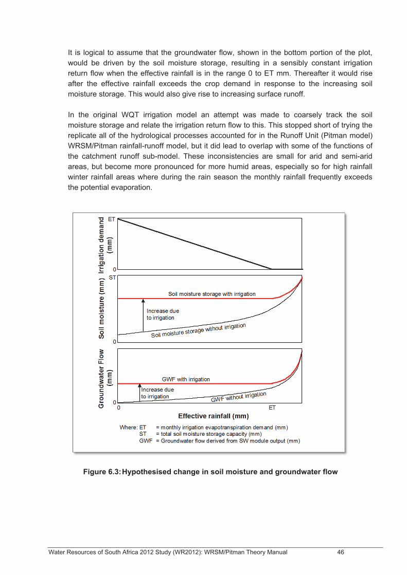
Water Resources of South Africa 2012 Study (WR2012): WRSM/Pitman Theory Manual 46
It is logical to assume that the groundwater flow, shown in the bottom portion of the plot, would be driven by the soil moisture storage, resulting in a sensibly constant irrigation return flow when the effective rainfall is in the range 0 to ET mm. Thereafter it would rise after the effective rainfall exceeds the crop demand in response to the increasing soil moisture storage. This would also give rise to increasing surface runoff. In the original WQT irrigation model an attempt was made to coarsely track the soil moisture storage and relate the irrigation return flow to this. This stopped short of trying the replicate all of the hydrological processes accounted for in the Runoff Unit (Pitman model) WRSM/Pitman rainfall-runoff model, but it did lead to overlap with some of the functions of the catchment runoff sub-model. These inconsistencies are small for arid and semi-arid areas, but become more pronounced for more humid areas, especially so for high rainfall winter rainfall areas where during the rain season the monthly rainfall frequently exceeds the potential evaporation.
Figure 6.3: Hypothesised change in soil moisture and groundwater flow

Water Resources of South Africa 2012 Study (WR2012): WRSM/Pitman Theory Manual 47
Modified WQT irrigation return flow The modified WQT irrigation module is aimed at redressing these problems and at the same time to reduce the complexity of some of the algorithms. The modified version uses the following guiding principles:
• The irrigation module and the catchment rainfall-runoff module (Salt Washoff (SW) module in the WQT model) should not overlap one another’s functions in the generation of runoff;
• The irrigation module must account for the increase in groundwater flow attributable to the irrigation application and
• The irrigation return flow needs to be spread more uniformly over time when the effective rainfall is less than the crop demand.
Two basic approaches could perform these functions:
• Excise the irrigated area entirely from the SW module and develop a comprehensive irrigation module for this area that encompasses all rainfall-runoff processes and irrigation processes and
• Use the SW model to account for rainfall-runoff processes and add the effect of irrigation application.
The first approach would offer a comprehensive solution and could be based on the Pitman model, with irrigation application simply acting as an enhanced rainfall to the irrigated sub-catchment. However, this approach would require solving the problem of relating potential evaporation values used in the Pitman model to the crop demand factors used for irrigation. Moreover, it must be recognised that the WQT model not only has to be able to be calibrated; its algorithms also have to be used in the WRPM, which uses stochastically generated runoff as its primary driving force. Hence an observed rainfall dataset will not always be available to drive a rainfall-runoff modelling process. For these reasons the second approach was adopted. Figure 6.4 shows the assumed water fluxes and storages used in the irrigation module. The variables used are defined in the following sections. Irrigation return flow associated with irrigation application The return flow associated with the irrigation application is made up of the following components:
• Return flow from upper soil zone;
• Return flow from lower soil zone;
• Loss to deep-seated groundwater and
• Spillage from ends of furrows and canals.
Water Resources of South Africa 2012 Study (WR2012): WRSM/Pitman Theory Manual 48
The applied irrigation water is assumed to enter into a store that gives rise to irrigation return flow and seepage to deep groundwater. This store is coarsely analogous to, but not identical with, the soil moisture storage. The processes governing the water balance of the normal (un-irrigated) portion of the catchment are already implicitly included in the catchment runoff used as input to the SW module and used as input to the irrigation module. The irrigation module treats the additional irrigation application separately. This approximation is necessary since any attempt to link the return flow to the entire soil moisture storage would inevitably result in duplication of the function of the SW module, thereby resulting in over-estimation of the runoff from the irrigated area. It must also be recognised that the inefficiency of the irrigation process (see Section 6.6.2) means that when the full irrigation demand is satisfied the total amount of water entering the irrigated land can substantially exceeds the crop demand and the observed return flow. Rigorous modelling of the irrigated land would of necessity mean having to account for this additional water loss. This is beyond the scope of this simplified irrigation model. (Nor does it appear to have been addressed adequately in most other irrigation models.) Aside from addressing the above factors, the modified WQT model needs to account for the fact that the full irrigation requirement is not always met, for the reasons given in Section 4.1.5. The land could also lie fallow for part of the year. During such conditions a drop in the irrigation-induced return flow can be expected, and this must be completely exhausted when irrigation ceases. To account for this the concept has been introduced of a pseudo tank to store the irrigation supply less the net crop demand and irrigation return. This is roughly analogous to the soil moisture storage, ignoring the effect of normal catchment processes, which are accounted for by the SW module.
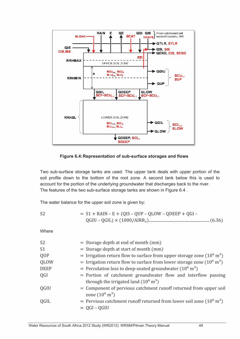
Water Resources of South Africa 2012 Study (WR2012): WRSM/Pitman Theory Manual 49
Figure 6.4: Representation of sub-surface storages and flows
Two sub-surface storage tanks are used. The upper tank deals with upper portion of the soil profile down to the bottom of the root zone. A second tank below this is used to account for the portion of the underlying groundwater that discharges back to the river. The features of the two sub-surface storage tanks are shown in Figure 6.4 . The water balance for the upper soil zone is given by:
Where
Water Resources of South Africa 2012 Study (WR2012): WRSM/Pitman Theory Manual 50
By the above definitions equation (6.36) can be simplified since the term QGI – QGIU – QGIL = 0. However, these terms have been retained since they assume significance in the salinity calculations (described in Section 4.3). The total return flow associated with the irrigation application, QIOUT (=QUP+QLOW) (10m³), is assumed to cease when the soil storage drops to RRHMIN:
Where
It must be recognised that through using crop factors the irrigation module deals with evapotranspiration differently to the ration the catchment modelling. As a result the modelled irrigation return flows are a simplifying approximation. Equations (6.36) and (6.37) applicable for estimating the additional sub-surface return flow associated with the irrigation for months when irrigation application actually takes place. This actually overlaps the groundwater flow component of the catchment runoff time series used as input to the Salt Washoff (SW) module. Calibration of the RRLF parameter provides a means of adjusting the net irrigation return flow to match the observed runoff at downstream river and reservoir gauging stations. However, during months when crop factors are low and/or the rainfall is high enough to satisfy the irrigation demand (i.e. when QIS is zero) it is necessary to avoid duplication of the excess runoff generated by the catchment runoff module. Since the irrigation module does not deal with the more complex rainfall-runoff processes and this is accommodated by the catchment runoff time series used as input to the Salt Washoff (SW) module. In fact, after a period of zero irrigation application the runoff from the irrigated portion of the land should behave much like any other part of the wider catchment. This effect can be accommodated by setting the irrigation return flow to zero when QIS drops to zero. (The normal catchment runoff time series would then fully account for the runoff.) However, doing so would imply an abrupt discontinuity in the soil moisture storage in the irrigation area. In reality, before the onset of the excess rain event the soil moisture would start off higher than that in the natural catchment, thereby causing an increase in runoff at the start of the wetter period, with the difference declining under the influence of evapotranspiration (or disappearing rapidly after the soil moisture storage capacity is exceeded). A simple means of mimicking this effect on the net return flow is to artificially set the rainfall input to zero. This causes the net influence of the irrigation on soil moisture storage (and hence return flow) to decline smoothly in a more realistic fashion.
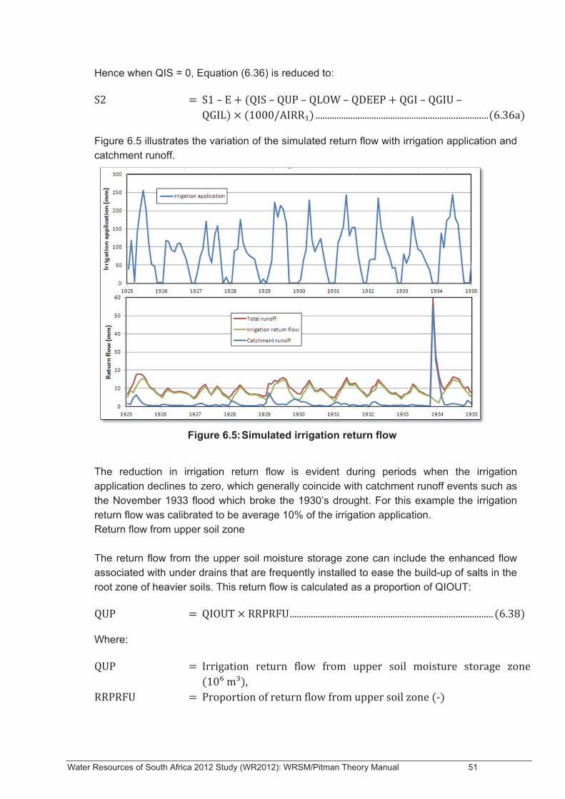
Water Resources of South Africa 2012 Study (WR2012): WRSM/Pitman Theory Manual 51
Hence when QIS = 0, Equation (6.36) is reduced to:
Figure 6.5 illustrates the variation of the simulated return flow with irrigation application and catchment runoff.
Figure 6.5: Simulated irrigation return flow
The reduction in irrigation return flow is evident during periods when the irrigation application declines to zero, which generally coincide with catchment runoff events such as the November 1933 flood which broke the 1930’s drought. For this example the irrigation return flow was calibrated to be average 10% of the irrigation application. Return flow from upper soil zone The return flow from the upper soil moisture storage zone can include the enhanced flow associated with under drains that are frequently installed to ease the build-up of salts in the root zone of heavier soils. This return flow is calculated as a proportion of QIOUT:
Where:
Water Resources of South Africa 2012 Study (WR2012): WRSM/Pitman Theory Manual 52
Return flow from lower soil zone The lower zone return flow attributable to irrigation application, QLOW (10 m³), is given as:
Where
The lower zone storage is important because this storage can bring about a long-term delay in the impact of irrigation schemes on river water quality. A case in point is the Vaalharts irrigation scheme, where the gradual build-up of salts in the irrigated lands took from the mid-1930s to the mid-1970s before the large scale installation of under drains was justified. Similar effects where observed at the massive Indus River irrigation scheme, which was commission at about the same time. Not only must this storage zone account for the groundwater directly under the irrigated lands and above the river level, it also needs to account for the transmission zone between lower edge of the irrigated land and the receiving stream. For this reason the storage depth, RRHSL (mm), can be quite deep. Loss to deep seated groundwater Part of the irrigation application can cause enhanced loss of water to deep-seated groundwater. This is particularly important for semi-arid and arid areas, which apply to many of the South African irrigation schemes. In such areas the regional water table is often lower than the invert level of local steams. This means that under normal conditions the percolation to groundwater is effectively lost. Irrigation activities have the effect of generating an artificial but sustained hump in the groundwater beneath and adjacent to the irrigated area. This causes an irrigation return flow to reach the stream (e.g. the QUP and QLOW components in Figure 6.4). However, there is also a net loss of water to the original widespread deep-seated groundwater table adjacent to the irrigated area. Numerous modelling studies showed the importance of taking this into consideration. For example a study of the Vaalharts irrigation scheme showed that 65% of the salt contained in the irrigation water supplied to the scheme between 1935 and 1990 had not left via return flow to the Harts River (Herold and Bailey, 1996). Similar effects have been found in numerous studies. This was handled in the original WQT irrigation model using parameter RRPSL. However, the value of parameter RRSCF also had to be carefully adjusted to prevent illogical sub-surface salt concentrations from occurring in the upper and lower soil zones. The modifications result in a much more stable solution. The deep percolation water loss is calculated as:
Where
Water Resources of South Africa 2012 Study (WR2012): WRSM/Pitman Theory Manual 53
The loss to deep-seated groundwater thus varies in proportion to the return flow to the surface water but is in addition to it. The total evapotranspiration loss from the upper soil moisture zone, E (mm), is assumed to bear a linear relationship with the soil moisture storage:
Where APANF is the monthly pan factor to convert A-pan evaporation to lake evaporation. S2 is solved from equations (6.36), (6.37), (6.38), (6.39), (6.40) and (6.41) as:
Where:
If the ending storage given by Equation (6.42) is less than RRHMIN, then set:
The implicit assumption is that when the storage declines to this value the irrigation evapotranspiration demand will be reduced accordingly due to the unavailability of water in the soil profile. Typically this condition could arise when the irrigation supply, QIS, remains lower than the net crop demand due to supply constraints. In effect the irrigation supply is then too small to sustain the irrigated area. An upper limit to the storage is also set. This is done to prevent unrealistically high storages from occurring during particularly wet periods.
Where
Water Resources of South Africa 2012 Study (WR2012): WRSM/Pitman Theory Manual 54
Under such conditions the enhanced catchment sub-surface flow is already accommodated by the SW module’s surface and sub-surface flow components. For this reason the excess water (QE) is taken as evaporation, since to include it in the return flow would duplicate the surface runoff component. It is recommended that RRHMAX should be set at the soil moisture storage capacity. For a well-balanced irrigation scheme this would result in a relatively constant irrigation return flow, which would drop significantly below the optimum target level during periods of supply restriction, or if the irrigation stops for a few months while the land lies fallow. High S2 values could also occur when the irrigation efficiency is low, since under such conditions the quantity of water applied to the land would substantially exceed the crop demand plus return flow. The assumption in such cases is that the surplus water will result in enhanced evapotranspiration loss. This is a reasonable assumption since water logging often accompanies over-irrigation due to inefficient practices. In the salinity modelling this will automatically reflect in increased soil salinity due to the increased evapotranspiration loss. This is also consistent with over-irrigation. The return flow resulting from the irrigation application is then calculated using Equations (6.37), (6.38) and (6.39). The method of application ensures that the irrigation return flow cannot exceed a fixed proportion of the applied irrigation water, and can decline below this when there is insufficient irrigation application to meet the crop demand. The enhanced groundwater flow attributable to normal catchment processes derived from the SW module is superimposed on this. Irrigation return flow associated with catchment runoff In this approach the catchment rainfall-runoff module (the Salt Washoff (SW) module in the WQT model) is assumed to provide the unit surface and groundwater flow associated with the rainfall on the irrigated portion of the catchment. An improvement here is that the SW module, which reads in a previously prepared catchment runoff file, uses algorithms to split the hydrograph into groundwater/interflow and surface flow runoff components. The surface runoff component of the catchment runoff rising from the irrigated portion of the catchment, QSI (10 m³), is assumed to simply enter the irrigation module return flow route without passing through the irrigated soil and is calculated as:
Where:
The groundwater flow component, QG (10 m³), from the irrigated portion of the catchment is assumed to enter the irrigated soil and exit as part of the simulated return flow. This is an approximation to mimic the groundwater flow associated with normal catchment processes:
Water Resources of South Africa 2012 Study (WR2012): WRSM/Pitman Theory Manual 55
QGI is the minimum irrigation return flow, to which is added the contribution associated with the irrigation application. This is a contra item since it is entered into the irrigated land and is returned back to the surface runoff. Hence, it is flow neutral and does not affect the pervious catchment runoff entered as part of the SW module input. In addition, the groundwater flow/interflow portion of the catchment runoff is also routed through the irrigated land to account for the normal rainfall-runoff processes. None of this water is lost, since the end result should preserve the flows originally modelled by the SW module.
Where QGIU (10 m³) is the portion of the catchment groundwater flow/interflow leaving the upper soil zone. The portion leaving via the lower soil zone is given by:
Where QGIL (10 m³) is the portion of the catchment groundwater flow/interflow leaving the Lower soil zone. Total irrigation return flow The total return flow to the irrigation return flow route is then given as:
Where QIR (10 m³) is the total flow to the irrigation return flow route.
Water Resources of South Africa 2012 Study (WR2012): WRSM/Pitman Theory Manual 56
7 GROUNDWATER (WITH 2005 ENHANCEMENTS) PITMAN MODEL VERSION 3 HUGHES (D A HUGHES, IWR, RHODES UNIVERSITY AND R PARSONS, PARSONS AND ASSOCIATES).
For both the Hughes method (this section) and the Sami method (refer to section G), groundwater modules have been designed to quantify the groundwater-surface water interaction at a quaternary catchment scale and have not been designed to quantify groundwater resources per se. At the quaternary catchment scale, it is necessary to simplify the use of some groundwater parameters such as transmissivity which could differ quite considerably from the stream bed to the rest of the quaternary catchment. For this reason, groundwater-surface water interactions at a scale smaller than quaternary catchment or at a river reach scale are more appropriately dealt with using existing finite element and finite difference models , for example FeFlow and Modflow.
7.1 Introduction
The first version of the revised Pitman model with more explicit ground water interaction routines was published in the Hydrological Sciences Journal during 2004 (Hughes, 2004). The original model focussed on the recharge and ground water discharge (to streamflow) components and assumed that the ground water level was always above the channel (or at the same level) The model has now been through several testing phases and development iterations to account for other processes and therefore should be applicable to more catchment situations than the first version. The additional components focussed on allowing for situations where the ground water level could drop below the river channel through riparian evaporation losses and sub-surface outflow to down-gradient catchments, as well as accounting for abstraction losses. One consequence of allowing for the ground water to drop below the channel was that channel transmission losses could play an important role in the overall water balance. As each component is described, some initial guidelines are provided for establishing parameter values and calibrating the new model parameters, as well as adjusting some of the original model parameters relative to the default values given in WR90. Many of these parameter estimation approaches are based on a data set of ground water variables compiled by Conrad (2005). These were supplied as integrated values for all the quaternary catchments in the country.
7.2 Recharge
The basis of the recharge component is that the surface characteristics can be represented by a single storage given that direct recharge can occur where there are bare rock areas. A parameter is required to represent the storage below which no recharge is expected to occur (soil water storage up to field capacity). The depth of recharge can then be estimated as a non-linear relationship with the ratio of current storage to the maximum storage (Equation 7.1).

Water Resources of South Africa 2012 Study (WR2012): WRSM/Pitman Theory Manual 57
The Pitman model already simulates soil moisture storage, while the SL parameter is normally set to zero and plays no real role in the current version of the model. The proposed restructuring therefore makes use of SL as the soil moisture threshold below which recharge does not occur, while its effect on runoff generated from soil moisture is removed. Parameter GW is redefined as the maximum amount of recharge (at a moisture status equal to ST) and a new parameter GPOW introduced to determine the form of the relationship between recharge and current storage S (Figure 7.1).
This function has remained the same throughout all the development phases.
7.2.1 Recharge calibration principles There are indications that the parameter SL can be fixed at 0, as the quantities of recharge at low soil moisture levels is normally small and not very important in the whole water balance. There are no direct methods of estimating GW and GPOW from a knowledge of the expected mean annual recharge. This is largely because of the highly non-linearity of the recharge process and its close association with the other outputs (interflow and evapotranspiration losses) from the soil water storage (S). It has been found that GPOW can be set to a fixed value of 3.0, after which GW is set to generate an ‘acceptable’ mean annual recharge value. Intuitively, it might be expected that the original model parameter FT, which determines the maximum amount of interflow, should reduce as the maximum recharge parameter (GW) is increased. The reasoning for this would be that in the original model interflow included ground water as a sub-component. Several tests suggest that FT should be reduced in some cases (mainly drier catchments), while in others it is not necessary to reduce this parameter. Inevitably, as the parameter GW is increased, outputs from the soil moisture store S are reduced, hence reducing interflow without modifying the FT value.
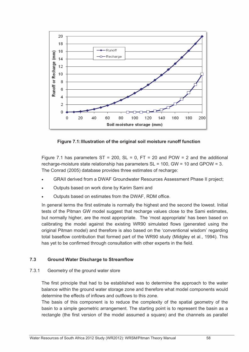
Water Resources of South Africa 2012 Study (WR2012): WRSM/Pitman Theory Manual 58
Figure 7.1: Illustration of the original soil moisture runoff function
Figure 7.1 has parameters ST = 200, SL = 0, FT = 20 and POW = 2 and the additional recharge-moisture state relationship has parameters SL = 100, GW = 10 and GPOW = 3. The Conrad (2005) database provides three estimates of recharge:
• GRAII derived from a DWAF Groundwater Resources Assessment Phase II project;
• Outputs based on work done by Karim Sami and
• Outputs based on estimates from the DWAF, RDM office.
In general terms the first estimate is normally the highest and the second the lowest. Initial tests of the Pitman GW model suggest that recharge values close to the Sami estimates, but normally higher, are the most appropriate. The ‘most appropriate’ has been based on calibrating the model against the existing WR90 simulated flows (generated using the original Pitman model) and therefore is also based on the ‘conventional wisdom’ regarding total baseflow contribution that formed part of the WR90 study (Midgley et al., 1994). This has yet to be confirmed through consultation with other experts in the field.
7.3 Ground Water Discharge to Streamflow
7.3.1 Geometry of the ground water store The first principle that had to be established was to determine the approach to the water balance within the ground water storage zone and therefore what model components would determine the effects of inflows and outflows to this zone. The basis of this component is to reduce the complexity of the spatial geometry of the basin to a simple geometric arrangement. The starting point is to represent the basin as a rectangle (the first version of the model assumed a square) and the channels as parallel

Water Resources of South Africa 2012 Study (WR2012): WRSM/Pitman Theory Manual 59
lines, separated by drainage slopes. The drainage slopes consist of the two areas between the edges of the rectangle and the outermost ‘channels’, plus two between each ‘channel’ line (Figure 7.2). Drainage is assumed to be 1-dimensional for simplicity. The determination of the number, length and width of the drainage slopes is therefore be based on the basin area and the effective drainage density. The channels included in the effective drainage density are those that can be considered to be the main recipients of ground water discharge and could exclude smaller tributary channels that are actively flowing only during storm events. Effectively drainage density is a model parameter that can be inferred (but probably not measured directly) from maps and an approximate understanding of the basin characteristics. The number of channel lines can be calculated from:
The ratio of catchment width/length is assumed to be related to Drainage density as follows:
Therefore:
By definition (and from Figure 7.2):
The number of drainage slopes is equal to 2 × number of channels, however Equation 7.5 has to be corrected to generate an even integer number of drainage slopes, each of which has a width given by:
Figure 7.3 illustrates the situation for a single drainage slope and the volume of the ‘wedge’ of ground water stored under that drainage slope (assuming that the lower boundary is the channel at the bottom of the slope) can be calculated as:
Where ‘Gradient’ is the hydraulic gradient of the ground water flowing toward the river channel (or away from the channel when the ground water is below the channel).
Outflows from this wedge to the river channel, within a single slope element can be calculated by:
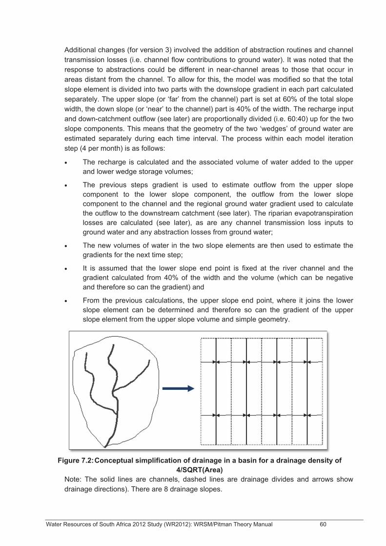
Water Resources of South Africa 2012 Study (WR2012): WRSM/Pitman Theory Manual 60
Additional changes (for version 3) involved the addition of abstraction routines and channel transmission losses (i.e. channel flow contributions to ground water). It was noted that the response to abstractions could be different in near-channel areas to those that occur in areas distant from the channel. To allow for this, the model was modified so that the total slope element is divided into two parts with the downslope gradient in each part calculated separately. The upper slope (or ‘far’ from the channel) part is set at 60% of the total slope width, the down slope (or ‘near’ to the channel) part is 40% of the width. The recharge input and down-catchment outflow (see later) are proportionally divided (i.e. 60:40) up for the two slope components. This means that the geometry of the two ‘wedges’ of ground water are estimated separately during each time interval. The process within each model iteration step (4 per month) is as follows:
• The recharge is calculated and the associated volume of water added to the upper and lower wedge storage volumes;
• The previous steps gradient is used to estimate outflow from the upper slope component to the lower slope component, the outflow from the lower slope component to the channel and the regional ground water gradient used to calculate the outflow to the downstream catchment (see later). The riparian evapotranspiration losses are calculated (see later), as are any channel transmission loss inputs to ground water and any abstraction losses from ground water;
• The new volumes of water in the two slope elements are then used to estimate the gradients for the next time step;
• It is assumed that the lower slope end point is fixed at the river channel and the gradient calculated from 40% of the width and the volume (which can be negative and therefore so can the gradient) and
• From the previous calculations, the upper slope end point, where it joins the lower slope element can be determined and therefore so can the gradient of the upper slope element from the upper slope volume and simple geometry.
Figure 7.2: Conceptual simplification of drainage in a basin for a drainage density of
4/SQRT(Area) Note: The solid lines are channels, dashed lines are drainage divides and arrows show drainage directions). There are 8 drainage slopes.
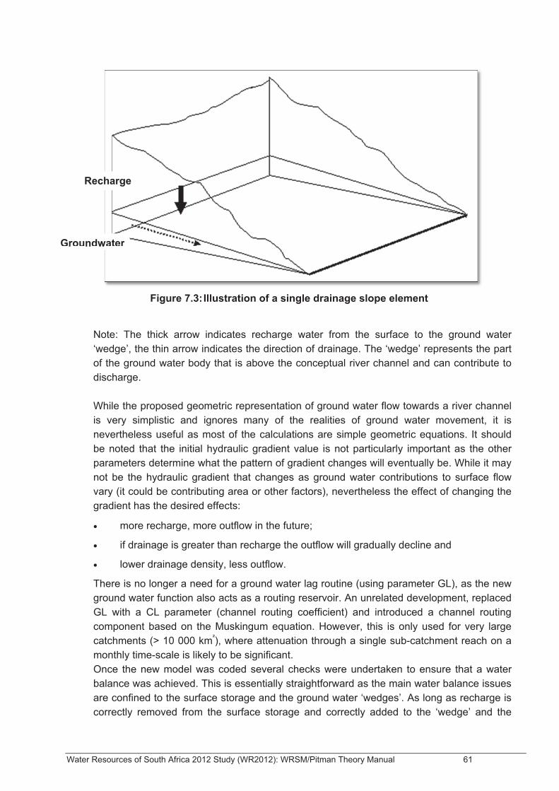
Water Resources of South Africa 2012 Study (WR2012): WRSM/Pitman Theory Manual 61
Figure 7.3: Illustration of a single drainage slope element
Note: The thick arrow indicates recharge water from the surface to the ground water ‘wedge’, the thin arrow indicates the direction of drainage. The ‘wedge’ represents the part of the ground water body that is above the conceptual river channel and can contribute to discharge. While the proposed geometric representation of ground water flow towards a river channel is very simplistic and ignores many of the realities of ground water movement, it is nevertheless useful as most of the calculations are simple geometric equations. It should be noted that the initial hydraulic gradient value is not particularly important as the other parameters determine what the pattern of gradient changes will eventually be. While it may not be the hydraulic gradient that changes as ground water contributions to surface flow vary (it could be contributing area or other factors), nevertheless the effect of changing the gradient has the desired effects:
• more recharge, more outflow in the future;
• if drainage is greater than recharge the outflow will gradually decline and
• lower drainage density, less outflow.
There is no longer a need for a ground water lag routine (using parameter GL), as the new ground water function also acts as a routing reservoir. An unrelated development, replaced GL with a CL parameter (channel routing coefficient) and introduced a channel routing component based on the Muskingum equation. However, this is only used for very large catchments (> 10 000 km²), where attenuation through a single sub-catchment reach on a monthly time-scale is likely to be significant. Once the new model was coded several checks were undertaken to ensure that a water balance was achieved. This is essentially straightforward as the main water balance issues are confined to the surface storage and the ground water ‘wedges’. As long as recharge is correctly removed from the surface storage and correctly added to the ‘wedge’ and the
Recharge
Groundwater
Water Resources of South Africa 2012 Study (WR2012): WRSM/Pitman Theory Manual 62
‘wedge’ volume correctly updated after drainage, there will be a water balance within the model. It should be noted that in some circumstances the ground water and surface water divides of a basin are not the same and regional ground water flows may dominate drainage processes. In such cases the model formulation would not be appropriate. This is not generally the case in the southern African region where fractured rock aquifers dominate. It was stated earlier that the initial value of the ground water gradient is not all that important as the model ‘warms up’ and determines gradient changes that are dependent on other parameters (GW, GPOW, storativity, transmissivity and drainage density). However, there can be problems interpreting the first few years of results if the starting value is very different to the valid range of gradients. To resolve this issue without adding a parameter for the starting value, the model is run twice. The starting gradients (upper and lower slope elements) in the first run is the regional ground water gradient (used for downstream outflows – see later), while the final gradients at the end of the first run become the starting gradients for the second model run.
7.3.2 Riparian losses to evapotranspiration It has been assumed that ground water can be subject to evapotranspiration losses close to the channel margin (either through use by riparian vegetation, or through evaporation from channel beds and banks). A model parameter has been added and is referred to as the Riparian strip factor. This is the percentage of the total slope element width over which evapotranspiration losses are assumed to occur and while the lower slope element gradient is greater than zero, the losses are assumed to occur at the potential evaporation rate. A further parameter (Rest water level – RWL) has been added that refers to the maximum depth below the channel that the connecting point between the upper and lower slope elements can reach before the ground water is considered to be inaccessible to all ground water outflow processes (discharge, abstractions and evapotranspiration). This depth is translated into a gradient (necessarily negative) that can be used to estimate a depletion factor, when the current lower slope element gradient is less than zero:
Evapotranspiration losses are reduced by this depletion factor (see Eq. 7.11). If there is a positive value for ground water discharge to the channel, this is first reduced by the evapotranspiration losses and if there are still losses to account for, the ground water volume (and hence the gradient) is reduced.
Net evaporation refers to the difference between potential evaporation demand and rainfall and negative values (i.e. where rainfall exceeds potential evaporation) are corrected to zero (to avoid duplicating the recharge function over the riparian strip).
Water Resources of South Africa 2012 Study (WR2012): WRSM/Pitman Theory Manual 63
7.3.3 Discharge to downstream catchments A regional ground water gradient parameter is included that refers to the gradient appropriate for estimating outflows from one sub-catchment to the next one downstream. The same basic flow equation (Eq. 7.9) is used:
The total outflow for a sub-catchment would then be the result of equation 7.11 times the number of slope elements. Clearly the influence of the drainage density on the catchment width/length ratio will have a major impact on the volume of downstream outflow. The outflow is reduced by the GW depletion factor (Eq. 7.10) when the lower slope element gradient is negative. Previous comments about the lack of correspondence between the surface and sub-surface water drainage systems need to be recognised. However, given the level of detail that is contained within the model, as well as the amount of information commonly available, it was not considered appropriate to add additional parameters that could account for differences in routes of water movement in the surface and sub-surface environments.
7.3.4 Parameter value estimation In summary the following new parameters have been added:
• transmissivity;
• storativity;
• drainage density;
• regional GW drainage slope;
• rest water level and
• riparian strip factor (% of slope width).
Transmissivity and storativity can be taken from the existing database of ground water parameters (Conrad, 2005) and only adjusted if the individual model user considers the database values to be incorrect or inappropriate for the specific study. The storativity value in the database can be used directly, while half the interpolated transmissivity values appear to be appropriate. Drainage density can be set at an initial value of 0.4 for most headwater catchments that do not have any specific shape characteristics. If they are elongated and the transmissivity parameter is high, it is probably sensible to reduce the drainage density (to 0.3 or even 0.2) to ensure that outflow volumes to the downstream catchment are not excessive. Reducing the drainage density can also be used to smooth the variations in ground water discharge to surface water (as can increasing the storativity). For downstream catchments, lower drainage densities appear to be appropriate (0.2 to 0.3). Note that drainage densities higher than about 0.5 should not be used unless there is extremely good justification.
Water Resources of South Africa 2012 Study (WR2012): WRSM/Pitman Theory Manual 64
The regional ground water slope does not seem to need to vary very much between catchments and provisional estimates suggest that a value of close to 0.01 will be satisfactory in most catchments. There is very little information available on this process at the scale of quaternary catchments and the drainage density parameter is likely to influence the volumes as much as any other parameter. The initial parameter estimates were based on the following equation where the catchment average slope values (as a percentage) in the Conrad (2005) database were greater than 1 (in other cases the GW drainage slope was taken as the catchment average slope/100:
The rest water level parameter can be taken from the existing database of ground water information (using the variable ‘median saturated thickness’, Conrad, 2005) and is not a very sensitive parameter in the model. However, extreme parameter values should be avoided (i.e. less than 10 m and greater than about 50 m) to avoid problems with the variation in the ground water depletion factor calculation.
7.4 Channel Losses and Ground Water Abstractions
The final changes incorporated into version 3 of the model involved the addition of abstraction routines and channel transmission losses (i.e. channel flow contributions to ground water). The addition of these new components was the main motivation for dividing each slope element into two parts; the upper (or far from the channel) and the lower (or close to the channel). To avid adding any new parameters the upper element is taken as 60% of the total slope element width, and the lower as 40%. The principles are that the water balance calculations are first performed on the lower slope component and the lower slope and position of the junction point fixed. The water balance calculations are then performed on the upper slope element and the gradient of the upper slope fixed for the start of the next time interval. An assessment of the differences between the single slope element version of the model and the revised, two element version, suggested that the two will give almost identical results when there are no abstractions and channel losses.
7.4.1 Channel transmission losses It was recognised that when the ground water level drops below the level of the channel (a negative downslope gradient in the model), it is possible that losses will occur from the channel back to the aquifer and that the rate of loss will be due to some characteristics of the channel (unknown), the head difference between the channel and the ground water and the transmissivity of the material under the channel. It is not really possible to estimate these in practical situations and it is also necessary to minimise the number of additional parameters (enough new parameters have already been added). It is also important to recognise that there are two components of channel loss in downstream catchments (i.e. where there are sub-catchments upstream that generate inflows into the current catchment being modelled). The first component is channel losses
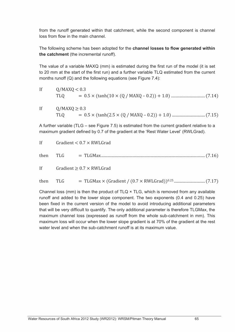
Water Resources of South Africa 2012 Study (WR2012): WRSM/Pitman Theory Manual 65
from the runoff generated within that catchment, while the second component is channel loss from flow in the main channel. The following scheme has been adopted for the channel losses to flow generated within the catchment (the incremental runoff). The value of a variable MAXQ (mm) is estimated during the first run of the model (it is set to 20 mm at the start of the first run) and a further variable TLQ estimated from the current months runoff (Q) and the following equations (see Figure 7.4):
A further variable (TLG – see Figure 7.5) is estimated from the current gradient relative to a maximum gradient defined by 0.7 of the gradient at the ‘Rest Water Level’ (RWLGrad).
Channel loss (mm) is then the product of TLQ × TLG, which is removed from any available runoff and added to the lower slope component. The two exponents (0.4 and 0.25) have been fixed in the current version of the model to avoid introducing additional parameters that will be very difficult to quantify. The only additional parameter is therefore TLGMax, the maximum channel loss (expressed as runoff from the whole sub-catchment in mm). This maximum loss will occur when the lower slope gradient is at 70% of the gradient at the rest water level and when the sub-catchment runoff is at its maximum value.
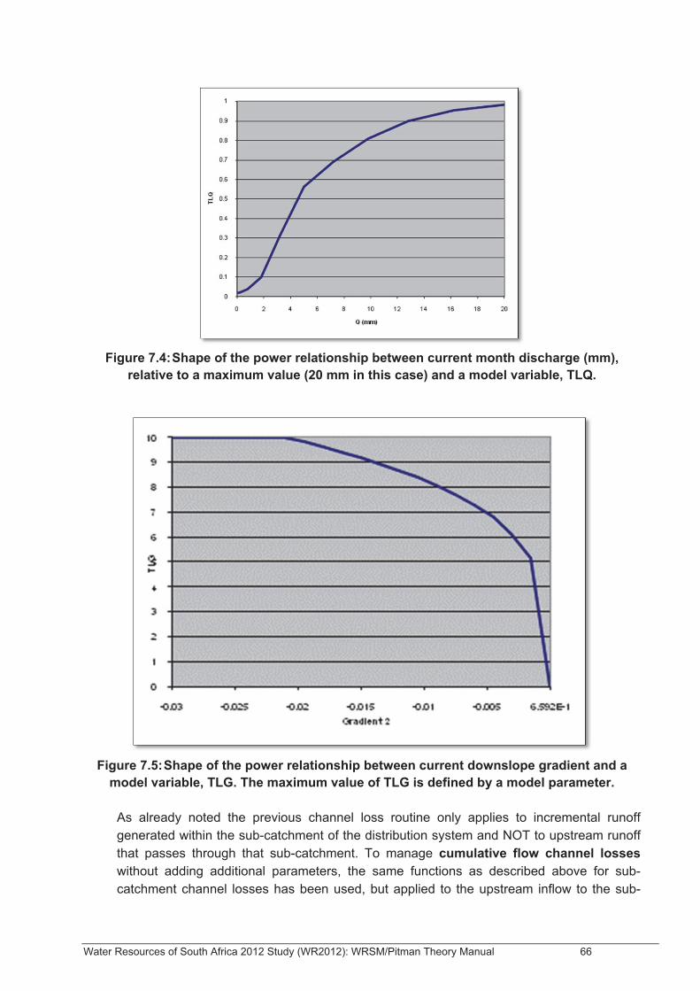
Water Resources of South Africa 2012 Study (WR2012): WRSM/Pitman Theory Manual 66
Figure 7.4: Shape of the power relationship between current month discharge (mm),
relative to a maximum value (20 mm in this case) and a model variable, TLQ.
Figure 7.5: Shape of the power relationship between current downslope gradient and a
model variable, TLG. The maximum value of TLG is defined by a model parameter. As already noted the previous channel loss routine only applies to incremental runoff generated within the sub-catchment of the distribution system and NOT to upstream runoff that passes through that sub-catchment. To manage cumulative flow channel losses without adding additional parameters, the same functions as described above for sub-catchment channel losses has been used, but applied to the upstream inflow to the sub-
Water Resources of South Africa 2012 Study (WR2012): WRSM/Pitman Theory Manual 67
catchment. The GW gradient component of the function remains the same (equations 7.16 and 7.17), except that TLGmax now represents a maximum channel loss from upstream inflow (in m³ × 10 ). TLGmax_Inflow is calculated from the TLGmax parameter for incremental flow using the following scheme:
Where MAXQ is defined previously as the maximum sub-area runoff (mm) and MAXQ_Inflow is the maximum upstream inflow. Both of these are set to initial values in the first run of the model (MAXQ = 20 mm, MAXQ_Inflow = 20 mm × cumulative upstream catchment area) and are then re-calculated for the second run from the data simulated during the first run. Equations 7.14 and 7.15 are also used to estimate the TLQ component, but with MAXQ replaced by MAXQ_Inflow and Q defined as the upstream inflow in any one month. The cumulative inflow channel losses are estimated at the start of a single months simulation and reduce the upstream inflow (there is no iteration of this calculation). The additional volume is then added to the near channel (or lower element) ground water storage in equal amounts over the model iteration steps (fixed at 4 in the current version of the model). Clearly, this function has no impact on headwater catchments that have no upstream inflow. There are potential problems with the function related to the simplified GW geometry as defined by the drainage density parameter and illustrated in Figure 7.2. The division of the catchment into slope elements represents all the channels, while upstream inflow losses should only apply to the main channel. However, in reality sub-catchments that experience significant main stem channel losses would probably not have internal catchment tributaries that are likely to generate GW flow. The assumption is that the effective channel network and drainage density for the purposes of GW-SW interaction would be made up only of the main channel. In that case the drainage density would be low and the ratio between catchment width and length also relatively low, which should be a reasonable reflection of reality.
7.4.2 Abstractions Abstractions are allowed for as annual volumes and seasonal distributions from both the near channel and remote environments. There are therefore two additional water use parameters which represent the abstraction volumes in m³ × 1000 from all the upper and lower slope elements. An additional column has also been added to the monthly distribution data requirement, which represents the seasonal distribution of GW abstractions (the same distribution is applied to both abstractions).
7.4.3 Parameter estimation The only additional parameter (apart from the abstraction volumes) is the TLGMax value which represents the maximum possible channel loss and is used for both the loss routines. This will always be a difficult parameter to quantify, but fortunately will only be relevant to a relatively small number of catchments in the country. However, it is important that this parameter is not ignored in dry regions where the ground water lower slope
Water Resources of South Africa 2012 Study (WR2012): WRSM/Pitman Theory Manual 68
element gradient will be nearly always negative. If the TLGMax parameter is set too high relative to simulated runoff depths it is possible that a large part of the runoff generated from other model components could be lost to ground water. The use of TLGMax for both loss functions might be considered problematic. However, where there are major losses from upstream runoff, there is likely to be very little incremental flow within the sub-catchment. The value of TLGMax will therefore be dominated by the range of values of upstream inflow, rather than local runoff.
7.5 Some Initial Observations
Several test runs of the revised version of the model have been assessed for the credibility of the results and the extent to which the model can reproduce the time-series of WR90 flows with minimal changes to the WR90 parameters. In terms of calibration, it was found that only small changes were necessary to the original WR90 parameters to achieve the same time series of flow as WR90 when ‘sensible’ ground water parameters were used in the model. The main parameter to change is the FT parameter (normally reduced as this already accounts for baseflow to a certain extent). In the arid areas tested no changes to the original model parameters were found to be necessary at this level of testing. An initial test of the abstraction components and the effects on the gradients within the two slope elements was undertaken on catchment X12A. Figure 7.6 indicates what happens in the model when there are no abstractions and when abstractions of 5 ×10 m³ are included from the upper and lower slope elements. The parameters of the model have been set as Transmissivity = 8 m² d-1, Storativity = 0.002. Recharge for the whole catchment is 8.487 × 10 m³ (or 5.092 over the upper element and 3.395 over the lower element). This means that the abstraction over the upper element represents almost all the recharge, while over the lower element it represents far more than the local recharge (but remember that the lower part is fed by downslope flow from the upper part).
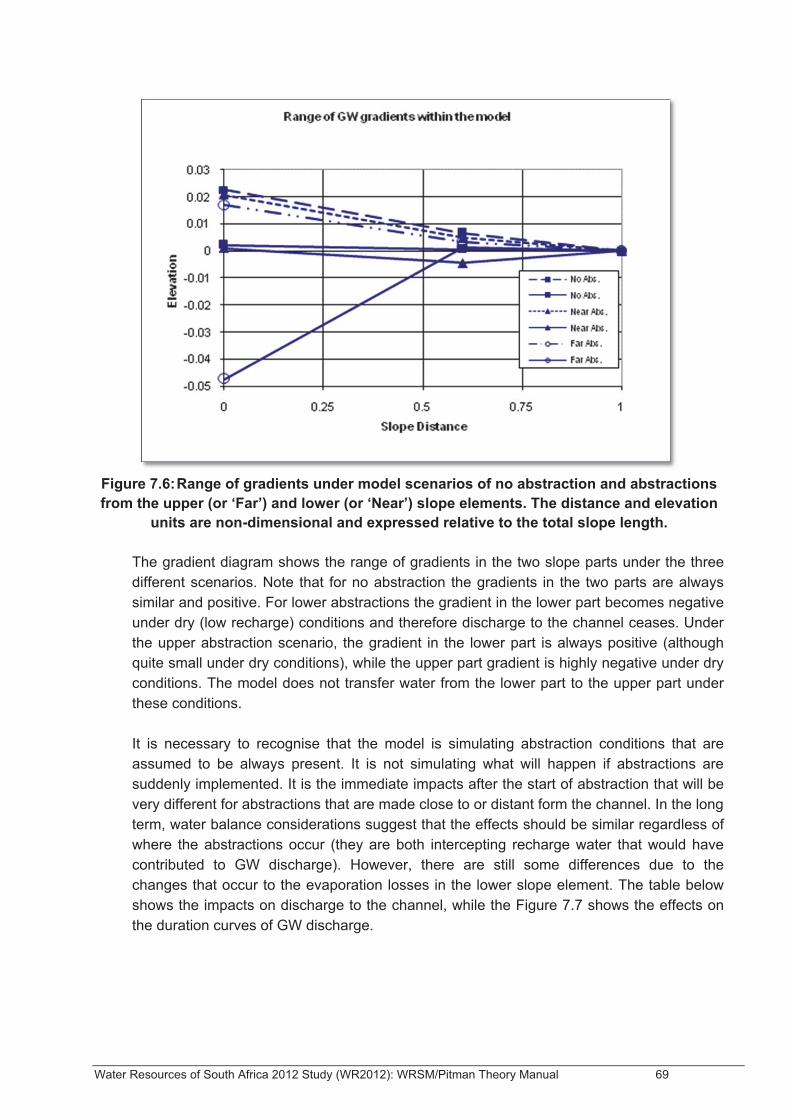
Water Resources of South Africa 2012 Study (WR2012): WRSM/Pitman Theory Manual 69
Figure 7.6: Range of gradients under model scenarios of no abstraction and abstractions from the upper (or ‘Far’) and lower (or ‘Near’) slope elements. The distance and elevation
units are non-dimensional and expressed relative to the total slope length. The gradient diagram shows the range of gradients in the two slope parts under the three different scenarios. Note that for no abstraction the gradients in the two parts are always similar and positive. For lower abstractions the gradient in the lower part becomes negative under dry (low recharge) conditions and therefore discharge to the channel ceases. Under the upper abstraction scenario, the gradient in the lower part is always positive (although quite small under dry conditions), while the upper part gradient is highly negative under dry conditions. The model does not transfer water from the lower part to the upper part under these conditions. It is necessary to recognise that the model is simulating abstraction conditions that are assumed to be always present. It is not simulating what will happen if abstractions are suddenly implemented. It is the immediate impacts after the start of abstraction that will be very different for abstractions that are made close to or distant form the channel. In the long term, water balance considerations suggest that the effects should be similar regardless of where the abstractions occur (they are both intercepting recharge water that would have contributed to GW discharge). However, there are still some differences due to the changes that occur to the evaporation losses in the lower slope element. The table below shows the impacts on discharge to the channel, while the Figure 7.7 shows the effects on the duration curves of GW discharge.
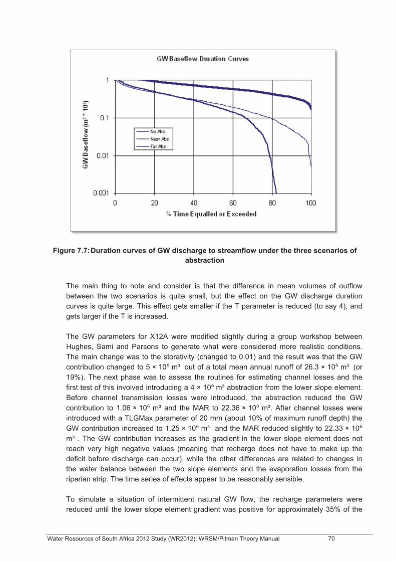
Water Resources of South Africa 2012 Study (WR2012): WRSM/Pitman Theory Manual 70
Figure 7.7: Duration curves of GW discharge to streamflow under the three scenarios of abstraction
The main thing to note and consider is that the difference in mean volumes of outflow between the two scenarios is quite small, but the effect on the GW discharge duration curves is quite large. This effect gets smaller if the T parameter is reduced (to say 4), and gets larger if the T is increased. The GW parameters for X12A were modified slightly during a group workshop between Hughes, Sami and Parsons to generate what were considered more realistic conditions. The main change was to the storativity (changed to 0.01) and the result was that the GW contribution changed to 5 × 10 m³ out of a total mean annual runoff of 26.3 × 10 m³ (or 19%). The next phase was to assess the routines for estimating channel losses and the first test of this involved introducing a 4 × 10 m³ abstraction from the lower slope element. Before channel transmission losses were introduced, the abstraction reduced the GW contribution to 1.06 × 10 m³ and the MAR to 22.36 × 10 m³. After channel losses were introduced with a TLGMax parameter of 20 mm (about 10% of maximum runoff depth) the GW contribution increased to 1.25 × 10 m³ and the MAR reduced slightly to 22.33 × 10m³ . The GW contribution increases as the gradient in the lower slope element does not reach very high negative values (meaning that recharge does not have to make up the deficit before discharge can occur), while the other differences are related to changes in the water balance between the two slope elements and the evaporation losses from the riparian strip. The time series of effects appear to be reasonably sensible. To simulate a situation of intermittent natural GW flow, the recharge parameters were reduced until the lower slope element gradient was positive for approximately 35% of the

Water Resources of South Africa 2012 Study (WR2012): WRSM/Pitman Theory Manual 71
time. Before introducing the channel loss parameter, the resulting MAR was simulated as 21.85 × 10 m³ with only 0.18 × 10 m³ being GW contribution. After introducing a TLGMax parameter of 20 mm, the MAR reduced to 21.62 × 10 m³ and the GW contribution increased to 0.41 × 10 m³, largely due to the fact that the lower element gradient now fluctuates around zero. Quaternary catchment Q92F was simulated using the standard WR90 regional parameters with a limited amount of recharge (2.7 mm from an MAP of 407 mm). Without channel losses, the upper element gradient varies around weakly positive values (0.5%), while the lower element gradient varies around –1.2%. The simulated MAR is 3.98 × 10 m³ and the maximum month runoff depth approximately 49 mm. Introducing a channel loss parameter (TLGMax) of 4 mm (10% of maximum monthly runoff depth), reduced the MAR to 2.99 × 10 m³. The lower element gradient now fluctuates over a wider range with an average of about –1%, while the effects on the upper element gradient is small but largely confined to more variation. The results appear to make intuitive sense, although in reality the WR90 parameters for the original model would now require some modification. In general terms the revised algorithms appear to be generating results that are intuitively realistic. However, guidelines for quantifying the new parameter values and re-evaluating some of the original parameter values still need to be established. It is also necessary to critically review the values of the two fixed-value power variables in the channel loss routines. REFERENCES Conrad, J (2005) Preparation and production of a series of GIS-base maps to identify areas where groundwater contributes to baseflow (WRC Project Number K5/1498). GEOSS Report No. G2005/02-1 Hughes, DA (2004) Incorporating ground water recharge and discharge functions into an existing monthly rainfall-runoff model. Hydrol. Sci. Journ. 49(2), 297-311. Midgley, D. C., Pitman, W. V. & Middleton, B. J. (1994) Surface Water Resources of South Africa 1990, vols I–VI. Water Research Commission Reports nos 298/1.1/94–298/6.1/94, Pretoria, South Africa.

Water Resources of South Africa 2012 Study (WR2012): WRSM/Pitman Theory Manual 72
8 GROUNDWATER (WITH WR2005 STUDY ENHANCEMENTS) BY K SAMI –
8.1 Introduction
8.1.1 Applicable Documents Project Charter – Groundwater Resource Assessment Phase II, DWAF, 2003 Groundwater-surface water interactions – Groundwater Resource Assessment Phase II Project 2003-150, Rep. 3Be, DWAF
8.1.2 Acronyms and Abbreviations Acronym/Abbreviation Definition
WSAM DWAF Water Situation Assessment Model
NGDB National Groundwater Database
WRYM Water Resources Yield Model
WR90 Surface Water Resources of South Africa 1990
WR2005 Surface Water Resources of South Africa 2005
WRSM/Pitman Revised version of the Pitman model utilised in WR90 and WR2005
DWAF Department of Water Affairs and Forestry
WARMS Water Use Licensing, Registration and Revenue Collection
8.2 Background
8.2.1 Background to the Project Since the abstraction of groundwater may impact on the availability of surface water resources through baseflow depletion, the integrated and sustainable management and development of water resources requires an understanding of the interactions between groundwater and surface water. In 2003 the DWAF embarked on the Phase II Groundwater Resource Assessment programme. The main objective of the programme was to develop methodologies and data that will support groundwater resource quantification per defined management unit. This programme was also tasked with supporting Integrated Water Resources Management, whose portfolio is to deliver relevant information on groundwater resources in support of Integrated Water Reserve Management. The Phase II programme comprised 5 projects, of which Project 3B, Groundwater-Surface Water Interactions, was one. The objective of this project was to review methods to quantify groundwater-surface water interactions and to develop a generic algorithm that can be applied to estimate groundwater-surface water interaction nationally on a quaternary catchment scale. Project 3B was divided into phases whereby:
• the international literature on assessing surface groundwater interactions would be reviewed;
Water Resources of South Africa 2012 Study (WR2012): WRSM/Pitman Theory Manual 73
• existing data sets available in South Africa would be identified;
• an algorithm to quantify interactions would be developed and
• a data base populated.
A methodology and algorithms were developed whereby the impacts on baseflow from groundwater abstraction and its proximity to river channels could be simulated. The methodology was incorporated into an MS-EXCEL environment. These algorithms were also coded into a multi worksheet MS-EXCEL data base set up by Quaternary catchment that was used to estimate interactions for over 1200 Quaternary catchments where baseflow occurs. Subsequently, the software found application in simulating the potential impacts of groundwater abstraction on the time series of baseflow for use in systems models to determine the potential impacts on reservoir yields and resource reliability. This led to discussions on the potential incorporation of the methodology into systems models, such as the Water Resources Yield Model, which currently only consider surface water abstractions. Modifications were also made to the software so that it could be incorporated into WR2005. The algorithms are currently being coded into the Pitman model in WR2005 in order to simulate baseflow nationwide. In addition to preliminary nationwide estimates of groundwater baseflow per Quaternary catchment in GRA II, the model has so far been applied in the following cases:
• Schoonspruit Eye: To determine the impacts of groundwater abstraction on flow from the eye, for the Reserve determination, and for use in WRYM to determine modifications to the yield of Johan Neser dam (DWAF);
• Middle Letaba: To determine the impacts of groundwater abstraction on inflows to the Middle Letaba Dam (DWAF) and
• Klein Dwars: To determine impacts on inflows to De Hoop dam from a proposed wellfield for Amplats in the Klein Dwars alluvium (AMPLATS).
The following investigations are also in progress:
• Mhlutuze Basin: revised baseflow simulations for the revision of the systems analysis of the W10 basin (DWAF) and
• Mokolo Basin: revised baseflow simulations for the revision of the systems analysis of the Mokolo A42 basin (DWAF).
8.2.2 Review of Groundwater-Surface Water Interactions Surface water and groundwater interactions can be classified as follows: Those involving contributions to streamflow :
• interflow occurring from the unsaturated zone contributing to hydrograph recession following a large storm event;
• groundwater discharged from the regional aquifer to surface water as baseflow to river channels, either to perennial effluent or intermittent streams;
Water Resources of South Africa 2012 Study (WR2012): WRSM/Pitman Theory Manual 74
• seepage to permanent or temporary wetlands;
• seepage from or to reservoirs and lakes and
• discharge from perched water tables via temporary or perennial springs located above low permeability layers, which may cause prolonged baseflow following rain events, even when the regional water table is below the stream channel.
Those involving losses from streamflow :
• transmission losses of surface water when river stage is above the groundwater table in phreatic aquifers with a water table in contact with the river;
• transmission losses in detached rivers, either perennial or ephemeral, where the water table lies at some depth below the channel and
• induced recharge caused by pumping of aquifer systems in the vicinity of rivers causing a flow reversal.
Those involving both losses and gains to streamflow depending on Stage are:-
• transmission losses of a temporary nature, recharging bank storage in alluvial systems during high flows, which are subsequently released to the channel during low flows.
The exchange of water between the surface and subsurface is a function of the difference between river stage and aquifer head. The direction of exchange varies with hydraulic head; however, the rate of exchange is also dependent on permeability properties. Seasonal variations in head may cause changes from effluent (groundwater draining into stream) to influent (surface water contributes to groundwater) conditions when higher hydraulic pressures exist in the stream channel due to storm runoff. The quantification of such interactions is necessary to avoid pitfalls such as double accounting of water resources. For example, hydrologists often consider baseflow as part of stream runoff, hence an allocatable surface resource. Geohydrologists often consider groundwater resources in terms of recharge, a large portion of which generates baseflow. Consequently, the simple addition of surface water runoff volumes and groundwater resources based on recharge (i.e. Harvest Potential) double accounts for the baseflow component. The quantification of these processes is severely hampered by miscomprehension of the terminologies used by hydrologists, ecologists and geohydrologists. Streamflow originating from subsurface pathways and contributing to baseflow is often all termed groundwater by hydrologists and ecologists, as well as some geohydrologists, which may lead to conceptual misunderstandings since not all these pathways incur passage through the regional aquifer. Subsurface water which does not flow through the regional aquifer is not available to boreholes in terms of conventional groundwater resource assessment; hence a distinction needs to be made between baseflow originating from the regional aquifer and baseflow originating from other subsurface pathways. Baseflow, as understood by ecologists and hydrologists, can be considered to consist of the portion of subsurface water which contributes to the low flow of streams. This can
Water Resources of South Africa 2012 Study (WR2012): WRSM/Pitman Theory Manual 75
originate from either: i) the regional groundwater body (groundwater baseflow), that portion of the total water resource that can either be abstracted as ground water or surface water, or; ii) saturated soils, perched aquifers, high lying springs, excess recharge that is not accepted by the aquifer, processes that can be lumped as interflow. In catchments with significant relief and geological heterogeneities, a large part of the baseflow fraction originates as interflow and never passes through the regional aquifer, and hence does not form part of the groundwater resources as considered in the concept of the groundwater Harvest Potential. Baseflow to maintain instream flows cannot, therefore, be simply attributed to discharge from the regional aquifers, since a large fraction could originate as interflow. The ecological significance of the regional aquifer when used as a groundwater resource would only be related to the connectivity of groundwater to the river reaches, and the degree to which the aquifer contributes baseflow. Groundwater abstraction may not impact at all on interflow from high lying springs, seeps, and perched water tables, hence would have no impact on the Ecological Reserve, or on the interflow component of baseflow in the river. Similarly, groundwater baseflow cannot be simply equated to recharge, since a portion of recharge may be lost in steep areas before reaching the regional aquifer through seepage of percolating water in outcropping fractures, springs draining perched water tables, artesian springs, evapotranspiration, or losses to deep lying regional groundwater which discharges at a great distance from the point of recharge. For these reasons, groundwater baseflow is very often significantly less than recharge, and similarly Exploitation or Harvest Potential are also much less than recharge. Therefore, it is not the recharge term that is significant when quantifying discharge of subsurface water into streams; only the fraction that re-emerges as baseflow is significant. Baseflow can be subdivided into: interflow not originating from the regional groundwater body and therefore not accessible by boreholes; and groundwater baseflow. Without a comprehension of such a distinction, the quantification of the impacts of groundwater abstraction cannot succeed. Only the portion of recharge re-emerging as groundwater baseflow can be impacted by abstraction. High lying perched springs would remain unaffected, unless land use or vegetation changes result in a reduction of springflow. Many publications (i.e. Rushton & Tomlinson, 1979) note that baseflow during hydrograph recession is not linearly related to hydraulic conductance, and during periods of high recharge, leakage calculated by models using linear means is much greater than occurs in practice. This can be attributed to ignoring increased hydraulic resistance to flow as discharge increases. This suggests linear methods, as incorporated in MODFLOW, do not provide a suitable avenue for modelling interactions in systems where large flow fluctuations occur, as is South African rivers. A more realistic approach to simulating interactions could be adopted by using non-linear equations whereby rapid increases in baseflow occur for small head changes when the head difference is small, but baseflow approaches some maximum value as the head difference becomes larger (Balleau, 1988).
Water Resources of South Africa 2012 Study (WR2012): WRSM/Pitman Theory Manual 76
Simulation of interactions is also relevant under conditions where groundwater abstraction takes place. The decline of water levels around pumping boreholes near surface water bodies creates gradients that capture some of the ambient groundwater that would have discharged as groundwater baseflow. At sufficiently high pumping rates these declines also induce flow out of the surface water body, a process known as induced recharge. Both these processes lead to streamflow depletion. The dynamics of stream depletion is thoroughly explained by Sophocleous (2002). Under natural conditions, dynamic steady-state conditions exist whereby in wet years recharge exceeds discharge and in dry years the reverse take place. This results in a cycle of rising and falling aquifer water levels. Pumping upsets this principle and new equilibrium conditions are eventually reached by increasing recharge (through induced recharge) or decreasing discharge (baseflow depletion, reduced groundwater outflow from the catchment, or reduced evapotranspiration losses from groundwater due to a lowering of water levels). Once new equilibrium conditions are reached whereby pumping is balanced by baseflow depletion a water licence to abstract groundwater is equivalent to a right to divert streamflow. In general, the further away the abstraction point is from the river, the longer the time to achieve equilibrium conditions. However, until equilibrium is reached these two volumes are not the same and the difference results in aquifer storage depletion. Therefore groundwater abstraction must consider both aquifer storage depletion and baseflow depletion and abstractions must be allocated in terms of the portion that originates as aquifer storage and that which comes from streamflow depletion. The length of time required for equilibrium to be reached between the surface water and groundwater flow depends on three factors: aquifer diffusivity, which is expressed as the ratio of aquifer storativity and transmissivity, the distance from the well to stream and the time of pumping. These are the three critical physical parameters affecting the impact of pumping on baseflows. In general, a tenfold increase in distance from a surface water course will result in a hundred fold increase in response time (Balleau, 1988). Recharge is unimportant in terms of the magnitude of the impact on baseflow; however, it limits the pumping rate since the portion originating from the aquifer cannot exceed recharge.
8.3 Proposed Methodology
8.3.1 Structure of methodology A logical stepped methodology was developed in a MS-Excel environment that determines the impacts of abstraction on baseflow. The methodology has been extended since GRA II to use two types of data inputs: 1) River hydrograph from which baseflow is separated using a hydrograph separation (Method 1); 2) time series of the Pitman S variable (subsurface storage), from which recharge is generated (Method 2). The two methods differ in the manner in which interflow is calculated. The hydrograph separation approach infers interflow as the difference between baseflow from the hydrograph separation and calculated groundwater baseflow. Baseflow can never exceed the original hydrograph discharge. The Pitman S approach calculates both interflow and groundwater baseflow independently of the catchment hydrograph. This approach was developed to remove the

Water Resources of South Africa 2012 Study (WR2012): WRSM/Pitman Theory Manual 77
subjective nature of hydrograph separations from the methodology, and to provide a direct link to the Pitman model.
The methodology is based on sequentially:
• either performing a hydrograph separation to separate groundwater baseflow (baseflow from the regional aquifer) and interflow (baseflow from perched aquifers) from storm runoff on a monthly time scale using WR90, observed flow data or a stochastic hydrograph;
• back calculating subsurface storage from the separated baseflow hydrograph to calculate a time series of recharge;
• or utilising the catchment soil moisture time series S generated by the WRSM/Pitman to calculate a time series of recharge;
• incrementing groundwater storage from recharge to a maximum aquifer capacity level, with any recharge in excess of aquifer capacity contributing to interflow;
• depleting groundwater storage by evapotranspiration and groundwater outflow to other catchments as a function of groundwater storage until static water level conditions are reached;
• calculating groundwater baseflow or transmission losses in a non-linear manner as a function of groundwater storage and runoff volume and
• depleting groundwater storage and groundwater baseflow due to abstraction as a function of aquifer diffusivity, time since pumping started, distance, and recharge.
The structure of the methodology is shown in Figure 8.1 and Figure 8.2 .
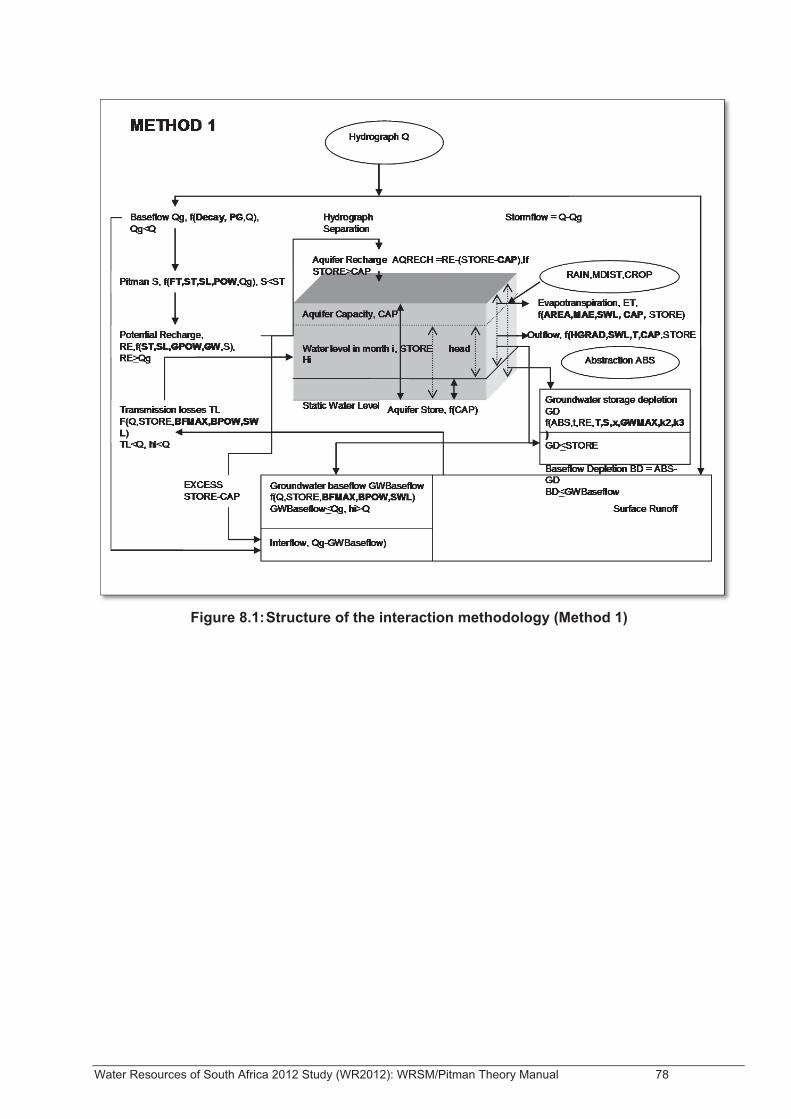
Water Resources of South Africa 2012 Study (WR2012): WRSM/Pitman Theory Manual 78
Figure 8.1: Structure of the interaction methodology (Method 1)
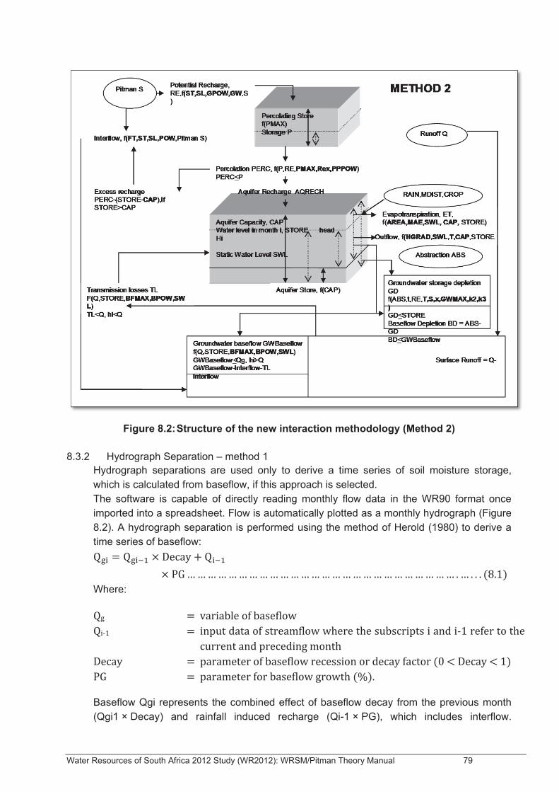
Water Resources of South Africa 2012 Study (WR2012): WRSM/Pitman Theory Manual 79
Figure 8.2: Structure of the new interaction methodology (Method 2)
8.3.2 Hydrograph Separation – method 1
Hydrograph separations are used only to derive a time series of soil moisture storage, which is calculated from baseflow, if this approach is selected. The software is capable of directly reading monthly flow data in the WR90 format once imported into a spreadsheet. Flow is automatically plotted as a monthly hydrograph (Figure 8.2). A hydrograph separation is performed using the method of Herold (1980) to derive a time series of baseflow:
Where:
Baseflow Qgi represents the combined effect of baseflow decay from the previous month (Qgi1 × Decay) and rainfall induced recharge (Qi-1 × PG), which includes interflow.

Water Resources of South Africa 2012 Study (WR2012): WRSM/Pitman Theory Manual 80
Parameters for PG and Decay are entered and adjusted to achieve a visual calibration. A monthly time series of baseflow is thereby generated. An error check is included to ensure that baseflow does not exceed total streamflow. The parameter Decay can be calibrated by comparing simulated baseflow to total streamflow during the driest period on record to ensure that simulated baseflow does not exceed or is significantly less than streamflow. Subsequently, PG is calibrated so that the baseflow hydrograph rises sufficiently to equal streamflow following large storm events. Results can also be calibrated against total baseflow volumes in the Situation Assessment Study of the Ground Water Resources of South Africa, or those in WSAM. The WSAM values produced by the Hughes SARES method are incorporated into the spreadsheet model via lookup tables based on Quaternary catchment number and can be used to assist with calibration. Separations can also be undertaken on observed gauging weir data, or stochastic hydrographs used by the WRYM model.
Figure 8.3: Hydrograph separation of the Klein Dwars Catchment, portion of B41G.
• Note: Area = 99 km², MAR = 8.38 Mm³/a, Baseflow = 2.57 Mm³ /a, DECAY = 0.75, GROWTH = 0.09
Once a hydrograph separation is obtained, the methodology calculates subsurface storage (Pitman S) by reverse engineering of the Pitman model (Coleman & Van Rooyen, pers. Comm., 2004):
POW
SLSTSLSFTQg
−−=
Where:
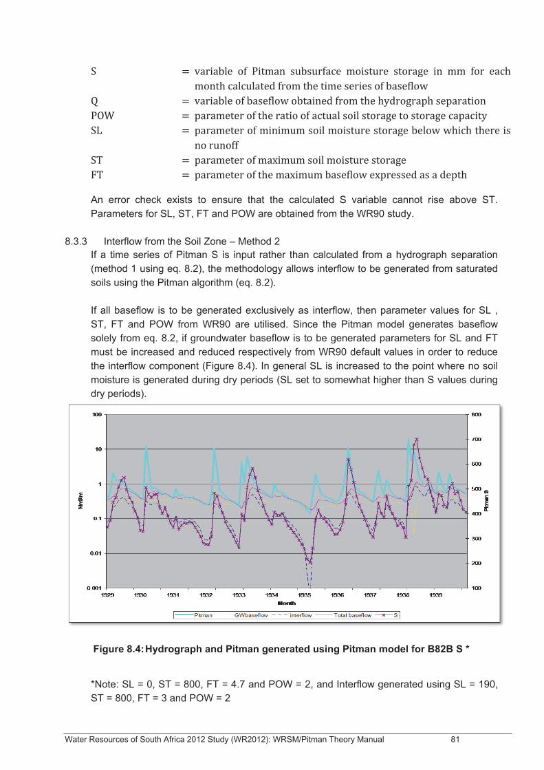
Water Resources of South Africa 2012 Study (WR2012): WRSM/Pitman Theory Manual 81
An error check exists to ensure that the calculated S variable cannot rise above ST. Parameters for SL, ST, FT and POW are obtained from the WR90 study.
8.3.3 Interflow from the Soil Zone – Method 2 If a time series of Pitman S is input rather than calculated from a hydrograph separation (method 1 using eq. 8.2), the methodology allows interflow to be generated from saturated soils using the Pitman algorithm (eq. 8.2). If all baseflow is to be generated exclusively as interflow, then parameter values for SL , ST, FT and POW from WR90 are utilised. Since the Pitman model generates baseflow solely from eq. 8.2, if groundwater baseflow is to be generated parameters for SL and FT must be increased and reduced respectively from WR90 default values in order to reduce the interflow component (Figure 8.4). In general SL is increased to the point where no soil moisture is generated during dry periods (SL set to somewhat higher than S values during dry periods).
Figure 8.4: Hydrograph and Pitman generated using Pitman model for B82B S *
*Note: SL = 0, ST = 800, FT = 4.7 and POW = 2, and Interflow generated using SL = 190, ST = 800, FT = 3 and POW = 2
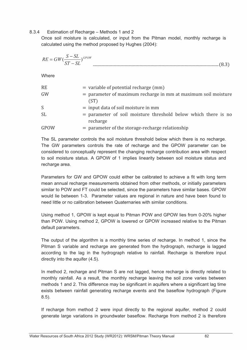
Water Resources of South Africa 2012 Study (WR2012): WRSM/Pitman Theory Manual 82
8.3.4 Estimation of Recharge – Methods 1 and 2 Once soil moisture is calculated, or input from the Pitman model, monthly recharge is calculated using the method proposed by Hughes (2004):
GPOW
SLSTSLSGWRE )(
−−=
Where
The SL parameter controls the soil moisture threshold below which there is no recharge. The GW parameters controls the rate of recharge and the GPOW parameter can be considered to conceptually represent the changing recharge contribution area with respect to soil moisture status. A GPOW of 1 implies linearity between soil moisture status and recharge area. Parameters for GW and GPOW could either be calibrated to achieve a fit with long term mean annual recharge measurements obtained from other methods, or initially parameters similar to POW and FT could be selected, since the parameters have similar bases. GPOW would lie between 1-3. Parameter values are regional in nature and have been found to need little or no calibration between Quaternaries with similar conditions. Using method 1, GPOW is kept equal to Pitman POW and GPOW lies from 0-20% higher than POW. Using method 2, GPOW is lowered or GPOW increased relative to the Pitman default parameters. The output of the algorithm is a monthly time series of recharge. In method 1, since the Pitman S variable and recharge are generated from the hydrograph, recharge is lagged according to the lag in the hydrograph relative to rainfall. Recharge is therefore input directly into the aquifer (4.5). In method 2, recharge and Pitman S are not lagged, hence recharge is directly related to monthly rainfall. As a result, the monthly recharge leaving the soil zone varies between methods 1 and 2. This difference may be significant in aquifers where a significant lag time exists between rainfall generating recharge events and the baseflow hydrograph (Figure 8.5). If recharge from method 2 were input directly to the regional aquifer, method 2 could generate large variations in groundwater baseflow. Recharge from method 2 is therefore
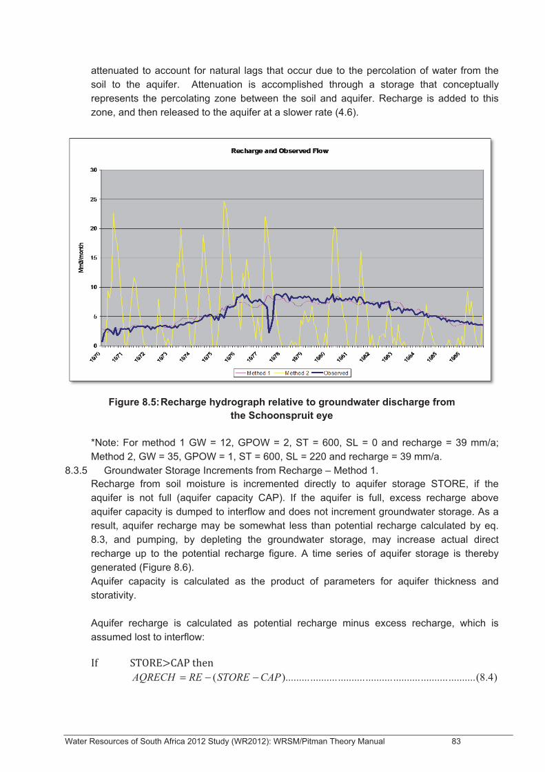
Water Resources of South Africa 2012 Study (WR2012): WRSM/Pitman Theory Manual 83
attenuated to account for natural lags that occur due to the percolation of water from the soil to the aquifer. Attenuation is accomplished through a storage that conceptually represents the percolating zone between the soil and aquifer. Recharge is added to this zone, and then released to the aquifer at a slower rate (4.6).
Figure 8.5: Recharge hydrograph relative to groundwater discharge from
the Schoonspruit eye *Note: For method 1 GW = 12, GPOW = 2, ST = 600, SL = 0 and recharge = 39 mm/a; Method 2, GW = 35, GPOW = 1, ST = 600, SL = 220 and recharge = 39 mm/a.
8.3.5 Groundwater Storage Increments from Recharge – Method 1. Recharge from soil moisture is incremented directly to aquifer storage STORE, if the aquifer is not full (aquifer capacity CAP). If the aquifer is full, excess recharge above aquifer capacity is dumped to interflow and does not increment groundwater storage. As a result, aquifer recharge may be somewhat less than potential recharge calculated by eq. 8.3, and pumping, by depleting the groundwater storage, may increase actual direct recharge up to the potential recharge figure. A time series of aquifer storage is thereby generated (Figure 8.6). Aquifer capacity is calculated as the product of parameters for aquifer thickness and storativity. Aquifer recharge is calculated as potential recharge minus excess recharge, which is assumed lost to interflow:
)4.8(............................................................).........( CAPSTOREREAQRECH −−=
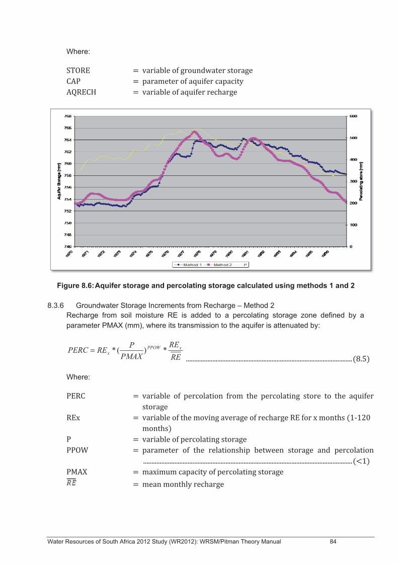
Water Resources of South Africa 2012 Study (WR2012): WRSM/Pitman Theory Manual 84
Where:
Figure 8.6: Aquifer storage and percolating storage calculated using methods 1 and 2
8.3.6 Groundwater Storage Increments from Recharge – Method 2
Recharge from soil moisture RE is added to a percolating storage zone defined by a parameter PMAX (mm), where its transmission to the aquifer is attenuated by:
RERE
PMAXPREPERC xPPOW
x *)(*=
Where:
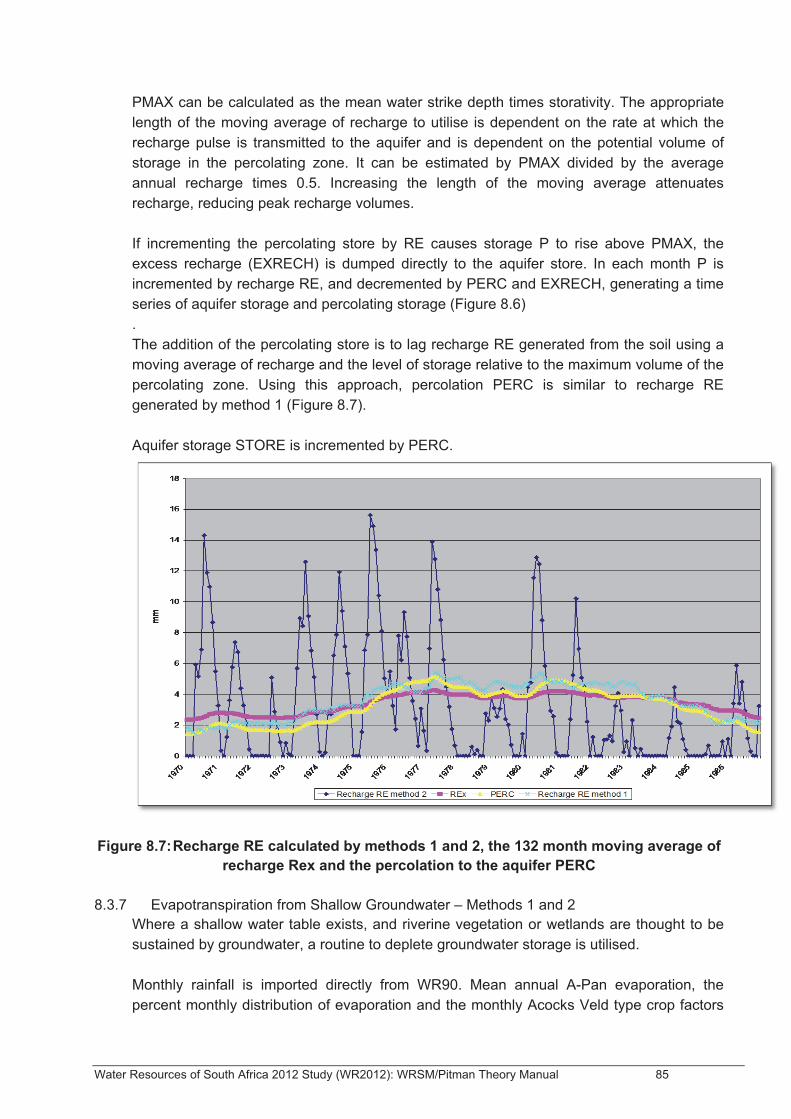
Water Resources of South Africa 2012 Study (WR2012): WRSM/Pitman Theory Manual 85
PMAX can be calculated as the mean water strike depth times storativity. The appropriate length of the moving average of recharge to utilise is dependent on the rate at which the recharge pulse is transmitted to the aquifer and is dependent on the potential volume of storage in the percolating zone. It can be estimated by PMAX divided by the average annual recharge times 0.5. Increasing the length of the moving average attenuates recharge, reducing peak recharge volumes. If incrementing the percolating store by RE causes storage P to rise above PMAX, the excess recharge (EXRECH) is dumped directly to the aquifer store. In each month P is incremented by recharge RE, and decremented by PERC and EXRECH, generating a time series of aquifer storage and percolating storage (Figure 8.6) . The addition of the percolating store is to lag recharge RE generated from the soil using a moving average of recharge and the level of storage relative to the maximum volume of the percolating zone. Using this approach, percolation PERC is similar to recharge RE generated by method 1 (Figure 8.7). Aquifer storage STORE is incremented by PERC.
Figure 8.7: Recharge RE calculated by methods 1 and 2, the 132 month moving average of recharge Rex and the percolation to the aquifer PERC
8.3.7 Evapotranspiration from Shallow Groundwater – Methods 1 and 2
Where a shallow water table exists, and riverine vegetation or wetlands are thought to be sustained by groundwater, a routine to deplete groundwater storage is utilised. Monthly rainfall is imported directly from WR90. Mean annual A-Pan evaporation, the percent monthly distribution of evaporation and the monthly Acocks Veld type crop factors
Water Resources of South Africa 2012 Study (WR2012): WRSM/Pitman Theory Manual 86
from WR90 are also entered, as is the area over which evapotranspiration can take place. Monthly evapotranspiration is calculated by the product of mean annual evaporation, monthly distribution and crop factor. Rainfall is subtracted from evapotranspiration to obtain evapotranspiration demand from groundwater. When rainfall exceeds evapotranspiration demand evapotranspiration from groundwater is defaulted to 0, since it is assumed that the evapotranspiration demand will be met from soil moisture storage. Evapotranspiration demand is multiplied by an aquifer storage factor to allow evaporation to decrease as groundwater storage is depleted. Evapotranspiration occurs at the maximum rate when groundwater storage is at aquifer capacity and declines towards 0 as groundwater storage drops to a level below the stream channel, defined by a parameter of static water level. Evapotranspiration from groundwater is therefore calculated by:
)/(**))**(( SWLCAPSWLSTOREAREARAINCROPMDISTMAE −−−
Where:
An error check is included to ensure evapotranspiration does not become negative if groundwater level drops below the static water level due to high levels of abstraction. Evapotranspiration is subsequently decremented from groundwater storage. CAP can be obtained from the Map of National Groundwater Resources Map of South Africa as the product of ‘Recommended Drilling Depth Below Groundwater Level’ and storativity. SWL is calculated as aquifer capacity less the degree of annual groundwater level fluctuation (in mm) times storativity. Hence the static water level can be expected to be 20-50 mm less than aquifer capacity, depending on the nature of the aquifer.
8.3.8 Groundwater Outflow – Methods 1 and 2 Groundwater is allowed to flow out of a catchment to simulate underflow and regional groundwater flow that does not emerge in surface water courses within the catchment. Groundwater outflow is calculated using the Darcian approach of the product of parameters of transmissivity T and the hydraulic gradient HG oriented out of the catchment. The hydraulic gradient fluctuates as a function of aquifer storage. The maximum hydraulic gradient is defined by a parameter HGRAD. This gradient is the hydraulic gradient oriented out of the catchment. The maximum value for HGRAD can be taken as the channel
Water Resources of South Africa 2012 Study (WR2012): WRSM/Pitman Theory Manual 87
gradient. The hydraulic gradient HG is decremented as the groundwater storage drops to the Static Water Level by:
)/(* SWLCAPSWLSTOREHGRADHG −−=
Where:
This format allows groundwater outflow to occur at a decreasing rate as the water level drops, until outflow stops when the static water level is reached. Groundwater outflow is allowed to become negative to simulate drawing in of water from adjacent catchments under conditions of large scale abstraction. Groundwater outflow is decremented from groundwater storage.
8.3.9 Groundwater Baseflow and Transmission losses – Methods 1 and 2 After evapotranspiration and groundwater outflow have been decremented from groundwater storage, groundwater baseflow is calculated. Groundwater baseflow is calculated as a function of the head difference between groundwater and surface water. Groundwater head in each month is calculated as the difference between STORE and SWL. Surface water head is calculated from the monthly runoff volume divided by catchment area. When groundwater head exceeds surface water head, as can occur during low flow months, groundwater baseflow is generated, simulating effluent conditions. These are decremented from groundwater storage. When surface water head exceeds groundwater head, as can occur during very wet months, temporary influent conditions arise and transmission losses to bank storage or to the aquifer are simulated. These are incremented to groundwater storage STORE. This system allows head differences to vary month by month due to both groundwater storage and streamflow variations, thereby overcoming problems based on assuming unrealistic constant head conditions in the river, as employed by MODFLOW. Groundwater baseflow (GWBaseflow) and transmission losses are calculated using a non-linear equation to account for the effects of hydraulic resistance:
BFMAXeGWBaseflow BPOWHEAD *)1( )( ×−=
Where:
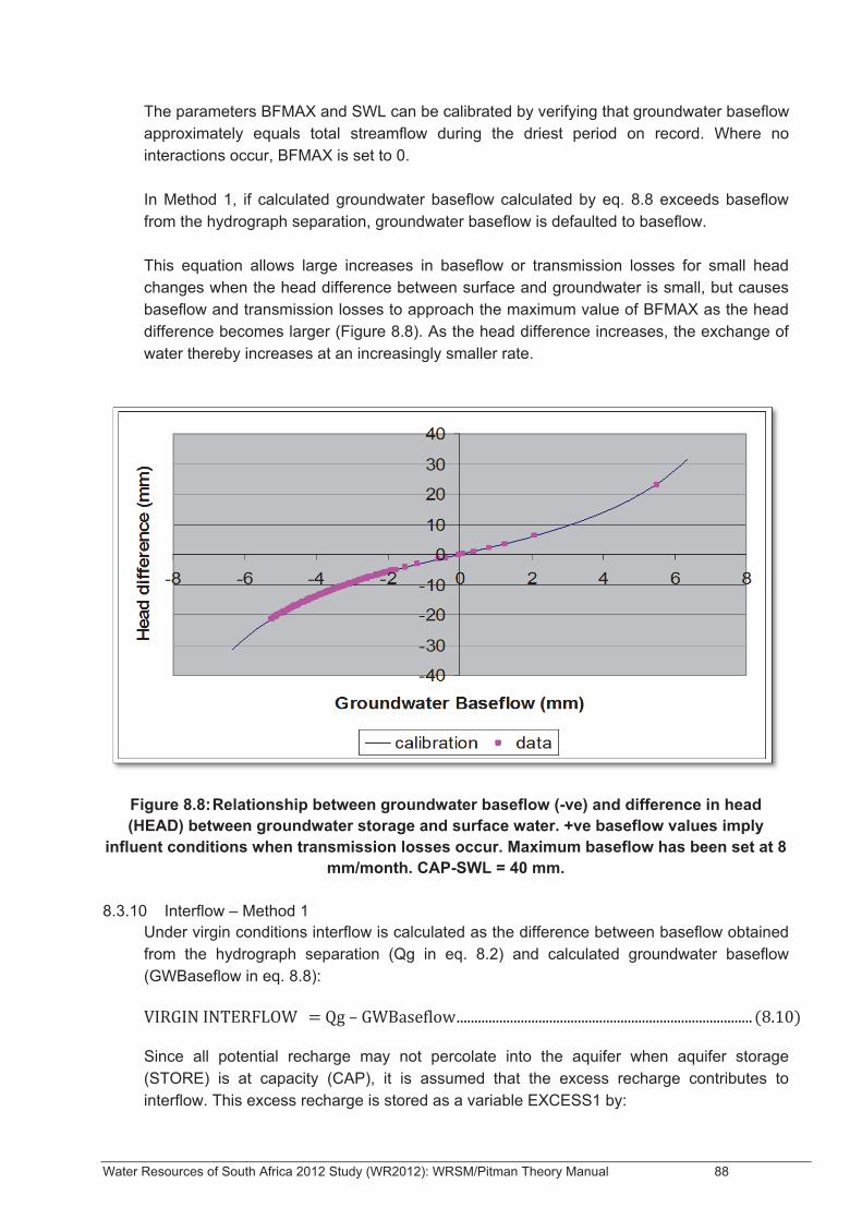
Water Resources of South Africa 2012 Study (WR2012): WRSM/Pitman Theory Manual 88
The parameters BFMAX and SWL can be calibrated by verifying that groundwater baseflow approximately equals total streamflow during the driest period on record. Where no interactions occur, BFMAX is set to 0. In Method 1, if calculated groundwater baseflow calculated by eq. 8.8 exceeds baseflow from the hydrograph separation, groundwater baseflow is defaulted to baseflow. This equation allows large increases in baseflow or transmission losses for small head changes when the head difference between surface and groundwater is small, but causes baseflow and transmission losses to approach the maximum value of BFMAX as the head difference becomes larger (Figure 8.8). As the head difference increases, the exchange of water thereby increases at an increasingly smaller rate.
Figure 8.8: Relationship between groundwater baseflow (-ve) and difference in head (HEAD) between groundwater storage and surface water. +ve baseflow values imply
influent conditions when transmission losses occur. Maximum baseflow has been set at 8 mm/month. CAP-SWL = 40 mm.
8.3.10 Interflow – Method 1
Under virgin conditions interflow is calculated as the difference between baseflow obtained from the hydrograph separation (Qg in eq. 8.2) and calculated groundwater baseflow (GWBaseflow in eq. 8.8):
Since all potential recharge may not percolate into the aquifer when aquifer storage (STORE) is at capacity (CAP), it is assumed that the excess recharge contributes to interflow. This excess recharge is stored as a variable EXCESS1 by:
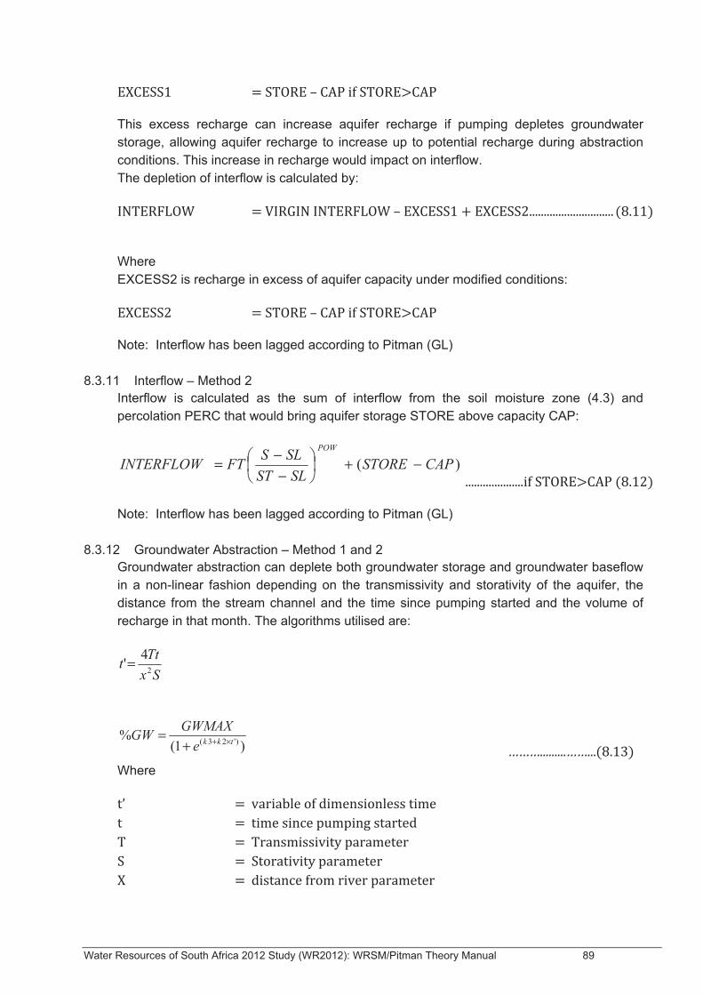
Water Resources of South Africa 2012 Study (WR2012): WRSM/Pitman Theory Manual 89
This excess recharge can increase aquifer recharge if pumping depletes groundwater storage, allowing aquifer recharge to increase up to potential recharge during abstraction conditions. This increase in recharge would impact on interflow. The depletion of interflow is calculated by:
Where EXCESS2 is recharge in excess of aquifer capacity under modified conditions:
Note: Interflow has been lagged according to Pitman (GL)
8.3.11 Interflow – Method 2 Interflow is calculated as the sum of interflow from the soil moisture zone (4.3) and percolation PERC that would bring aquifer storage STORE above capacity CAP:
)( CAPSTORESLST
SLSFTINTERFLOWPOW
−+−
−=
Note: Interflow has been lagged according to Pitman (GL)
8.3.12 Groundwater Abstraction – Method 1 and 2 Groundwater abstraction can deplete both groundwater storage and groundwater baseflow in a non-linear fashion depending on the transmissivity and storativity of the aquifer, the distance from the stream channel and the time since pumping started and the volume of recharge in that month. The algorithms utilised are:
SxTtt 2
4'=
)1(% )'23( tkke
GWMAXGW ×++=
Where
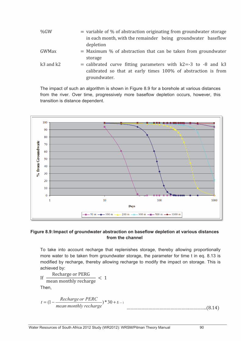
Water Resources of South Africa 2012 Study (WR2012): WRSM/Pitman Theory Manual 90
The impact of such an algorithm is shown in Figure 8.9 for a borehole at various distances from the river. Over time, progressively more baseflow depletion occurs, however, this transition is distance dependent.
Figure 8.9: Impact of groundwater abstraction on baseflow depletion at various distances from the channel
To take into account recharge that replenishes storage, thereby allowing proportionally more water to be taken from groundwater storage, the parameter for time t in eq. 8.13 is modified by recharge, thereby allowing recharge to modify the impact on storage. This is achieved by:
Then,
130*)1( −+−= it rechargemonthly meanPERC or Recharge t
Water Resources of South Africa 2012 Study (WR2012): WRSM/Pitman Theory Manual 91
13 t ,rechargemonthly mean
Recharge if i 1>
Then,
30*)( 1 rechargemonthly mean
Rechargei t t 1i −−= −
This algorithm allows an increased proportion of abstraction to be taken from groundwater store following recharge events exceeding the mean monthly recharge, and allows the transition to groundwater baseflow depletion to slow down during drier periods depending on the recharge volume. The depletion of groundwater baseflow (Depletion) is calculated by:
rechargemonthly meanPERC or Recharge* nsAbstractio* GW % 100 Depletion ii
001−=
The correction of Depletion by the ratio of recharge to mean monthly recharge allows the portion of recharge above the mean monthly value to replenish the accumulated aquifer storage deficit. This accounts for the fact that groundwater baseflow does not become evident following recharge events after prolonged abstraction due for the need to rewater the aquifer to some extent before baseflow can occur. The balance of abstraction volumes (abstraction-depletion) is taken from STORE. Depletion is subtracted from calculated groundwater baseflow (GWBaseflow), thereby depleting baseflow. If calculated baseflow depletion exceeds GWBaseflow, the excess is removed from groundwater storage (STORE). The volume taken from STORE would also cause increased transmission losses, due to a reduced groundwater HEAD.
8.4 Data Input
8.4.1 Parameters The parameters required and comments on the source of data are shown in Table 8.2.

Wat
er R
esou
rces
of S
outh
Afri
ca 2
012
Stu
dy (W
R20
12):
WR
SM
/Pitm
an T
heor
y M
anua
l 92
Tabl
e 8.
1: M
olde
com
pone
nts.
Par
amet
ers
used
onl
y in
met
hod
1 ar
e un
derli
ned.
Par
amet
ers
used
on
in m
etho
d 2
are
in It
alic
s.
1 P
= P
aram
eter
, I =
Initi
al c
ondi
tion,
D =
phy
sica
l dat
a, C
= c
alcu
late
d, T
= ti
me
serie
s in
put d
ata
Ite
m
Stat
us1
Sour
ce
Func
tion
Com
men
t C
omm
on R
ange
C
alib
ratio
n
CA
TCH
MEN
T C
HA
RA
CTE
RIS
TIC
S C
atch
men
t Are
a (C
ATC
HM
EN
T)
D
WR
90.
Vol
ume
and
flux
calc
ulat
ions
D
efau
lt va
lue
set f
rom
inte
rnal
look
up ta
ble
N
one
Aqu
ifer t
hick
ness
P
Nat
iona
l gro
undw
ater
reso
urce
s m
ap, N
atio
nal G
roun
dwat
er
data
base
, GR
A II
dat
a an
aqu
ifer
stor
age
Det
erm
ines
cap
acity
of a
quife
r (C
AP
). A
ffect
s E
vapo
trans
pira
tion,
gr
ound
wat
er b
asef
low
, gr
ound
wat
er o
utflo
w a
nd th
e ge
nera
tion
of in
terfl
ow a
s ex
cess
rech
arge
Bas
ed o
n di
ffere
nce
betw
een
SW
L an
d w
ater
stri
kes
in a
n aq
uife
r. C
an b
e re
gion
alis
ed b
y ge
olog
ical
dom
ain.
Mus
t be
mul
tiplie
d by
bor
ehol
e su
cces
s ra
tes
in c
atch
men
ts w
here
gr
ound
wat
er o
ccur
renc
e is
lim
ited
10-5
0 G
ener
ally
non
e. In
crea
sing
this
val
ue g
ener
ally
m
akes
gro
undw
ater
bas
eflo
w le
ss re
spon
sive
to
rech
arge
Sto
rativ
ity (S
) P
Nat
iona
l gro
undw
ater
reso
urce
s m
ap, N
atio
nal G
roun
dwat
er
data
base
, GR
A II
dat
a an
aqu
ifer
stor
age
Det
erm
ines
cap
acity
of a
quife
r. Im
pact
s on
tran
sitio
n fro
m
aqui
fer s
tora
ge to
bas
eflo
w
depl
etio
n du
ring
abst
ract
ion
Can
be
regi
onal
ised
by
geol
ogic
al d
omai
n 0.
001-
0.2
Incr
easi
ng th
is v
alue
gen
eral
ly m
akes
gro
undw
ater
ba
seflo
w le
ss re
spon
sive
to re
char
ge. I
t als
o re
sults
in
a lo
nger
tim
e de
lay
befo
re a
bstra
ctio
n im
pact
s on
ba
seflo
w
Aqu
ifer C
apac
ity
(CA
P)
C
Cal
cula
ted
inte
rnal
ly fr
om
Sto
rativ
ity a
nd a
quife
r thi
ckne
ss
Dep
ends
on
aqui
fer
thic
knes
s an
d st
orat
ivity
Initi
al g
roun
dwat
er
stor
e I
Cal
ibra
tion
In
itial
sto
rage
leve
l of a
quife
r
Cal
ibra
ted
so th
at lo
ng s
imul
atio
n un
der v
irgin
con
ditio
ns
resu
lts in
littl
e ch
ange
in s
tora
ge. I
f not
cal
ibra
ted
impa
ct o
n fin
al re
sults
is m
inim
al s
ince
cha
nge
in s
tora
ge o
ver l
ong
time
perio
d ha
s lit
tle im
pact
on
mea
n an
nual
val
ues
Bet
wee
n SW
L an
d C
AP
Usu
ally
set
hal
f way
bet
wee
n st
atic
wat
er le
vel a
nd
aqui
fer c
apac
ity. C
alib
rate
d so
that
Aqu
ifer S
tora
ge
Cha
nge
in th
e V
irgin
wat
er b
alan
ce is
app
roxi
mat
ely
zero
, ind
icat
ing
no c
hang
e in
sto
rage
ove
r the
long
te
rm
MA
P (R
AIN
) D
W
R90
C
ontro
ls e
vapo
trans
pira
tion
Use
d to
cal
cula
te m
onth
ly ra
infa
ll fro
m W
R90
mon
thly
rain
fall
dist
ribut
ion
files
Non
e
Sta
tic w
ater
leve
l (S
WL)
P
Cal
ibra
ted
regi
onal
ly. G
ener
ally
se
t to
CA
P –
sto
rativ
ity x
ann
ual
grou
ndw
ater
leve
l flu
ctua
tion
Con
trols
aqu
ifer s
tora
ge le
vel a
t w
hich
gro
undw
ater
bas
eflo
w,
evap
orat
ion
and
grou
ndw
ater
ou
tflow
term
inat
e
Can
be
regi
onal
ised
by
geol
ogic
al d
omai
n.
Mus
t be
less
than
CA
P. I
t is
gene
rally
mor
e th
an 5
0% o
f CA
P
in s
hallo
w o
r wea
ther
ed a
quife
rs a
nd h
ighe
r in
deep
sea
ted
fract
ured
aqu
ifers
with
littl
e ba
seflo
w
30-8
0% o
f CAP
Incr
easi
ng c
ause
s aq
uife
r to
rem
ain
full
and
grou
ndw
ater
bas
eflo
w to
term
inat
e as
aqu
ifer
dew
ater
s. R
educ
ing
resu
lts in
mor
e, le
ss
resp
onsi
ve a
nd m
ore
pers
iste
nt g
roun
dwat
er
base
flow
Uns
at S
tore
(P
MAX
) P
Cal
cula
ted
from
med
ian
dept
h to
w
ater
stri
ke ti
mes
sto
rativ
ity
Con
trols
rate
at w
hich
rech
arge
pe
rcol
ates
to a
quife
r U
sed
to la
g th
e tim
e be
twee
n re
char
ge a
nd th
e gr
ound
wat
er
base
flow
resp
onse
10
-400
In
crea
sing
cau
ses
rech
arge
to b
e m
ore
atte
nuat
ed
and
grou
ndw
ater
bas
eflo
w to
be
less
resp
onsi
ve
Initi
al S
tore
I
Cal
ibra
tion
In
itial
sto
rage
leve
l of
unsa
tura
ted
perc
olat
ing
stor
age
Cal
ibra
ted
so th
at lo
ng s
imul
atio
n un
der v
irgin
con
ditio
ns
resu
lts in
littl
e ch
ange
in u
nsat
urat
ed p
erco
latin
g st
orag
e. If
no
t cal
ibra
ted
impa
ct o
n fin
al re
sults
is m
inim
al s
ince
cha
nge
in s
tora
ge o
ver l
ong
time
perio
d ha
s lit
tle im
pact
on
mea
n an
nual
val
ues
Bet
wee
n 0-
PMA
X
Usu
ally
set
at a
bout
hal
f of P
MA
X. C
alib
rate
d so
th
at S
tora
ge C
hang
e is
app
roxi
mat
ely
zero
, in
dica
ting
no c
hang
e in
sto
rage
ove
r the
long
term
Mov
ing
aver
age
of
rech
arge
(Rex
) P
Cal
cula
ted
from
PM
AX
div
ided
by
mea
n m
onth
ly re
char
ge ti
mes
0.5
to
acc
ount
for r
esid
ual s
atur
atio
n.
Rec
harg
e va
lues
are
ava
ilabl
e fro
m G
RA
II
Con
trols
rate
at w
hich
rech
arge
pe
rcol
ates
to a
quife
r U
sed
to la
g th
e tim
e be
twee
n re
char
ge a
nd th
e gr
ound
wat
er
base
flow
resp
onse
1-
132
Incr
easi
ng c
ause
s re
char
ge to
be
mor
e at
tenu
ated
an
d gr
ound
wat
er b
asef
low
to b
e le
ss re
spon
sive

Wat
er R
esou
rces
of S
outh
Afri
ca 2
012
Stu
dy (W
R20
12):
WR
SM
/Pitm
an T
heor
y M
anua
l 93
Item
St
atus
1 So
urce
Fu
nctio
n C
omm
ent
Com
mon
Ran
ge
Cal
ibra
tion
HYD
RO
GR
APH
SEP
AR
ATI
ON
Dec
ay
P
Cal
ibra
ted
regi
onal
ly
Det
erm
ines
bas
eflo
w fr
om
hydr
ogra
ph s
epar
atio
n.
Con
trols
rate
of b
asef
low
re
cess
ion
on fa
lling
lim
b of
hy
drog
raph
Cal
ibra
ted
so th
at ‘b
asef
low
cal
cula
ted
is a
ppro
xim
atel
y eq
ual
to ‘M
ean
annu
al b
asef
low
’. Th
e pa
ram
eter
is g
ener
ally
hig
h (>
0.9)
in s
trong
ly b
asef
low
co
ntro
lled
river
s an
d lo
w (<
0.3)
in ri
vers
with
no
base
flow
or a
ve
ry ra
pid
shor
t dur
atio
n ba
seflo
w re
spon
se
0.3-
0.99
C
alib
rate
d by
obs
ervi
ng b
asef
low
dur
ing
drie
st
perio
d on
reco
rd. S
ettin
g it
too
low
cau
ses
too
low
a
base
flow
.
Gro
wth
P
C
alib
rate
d re
gion
ally
Det
erm
ines
bas
eflo
w fr
om
hydr
ogra
ph s
epar
atio
n.
Con
trols
rate
of b
asef
low
re
spon
se o
n ris
ing
limb
Cal
ibra
ted
so th
at ‘b
asef
low
cal
cula
ted
is a
ppro
xim
atel
y eq
ual
to ‘M
ean
annu
al b
asef
low
’. Th
e pa
ram
eter
is g
ener
ally
low
(<0.
05) i
n ca
tchm
ents
with
littl
e ba
seflo
w a
nd h
igh
(0.1
-0.2
) in
catc
hmen
ts w
ith s
igni
fican
t ba
seflo
w
0.05
-0.2
C
alib
rate
d so
that
‘bas
eflo
w c
alcu
late
d is
ap
prox
imat
ely
equa
l to
‘Mea
n an
nual
bas
eflo
w’.
Incr
easi
ng c
ause
bas
eflo
w to
incr
ease
.
Initi
al b
asef
low
I
Cal
ibra
ted
Sta
rting
con
ditio
n H
as v
ery
little
impa
ct o
n re
sults
as
it on
ly a
ffect
s ba
seflo
w
gene
rate
d in
firs
t mon
th.
<10%
of m
ean
annu
al
base
flow
N
ot c
alib
rate
d
Mea
n an
nual
ba
seflo
w
D
WS
AM
N
ot u
sed
in m
odel
In
clud
ed o
nly
as a
n ai
d in
cal
ibra
tion
of b
asef
low
vol
umes
. D
efau
lt va
lue
set f
rom
inte
rnal
look
up ta
ble
Bas
eflo
w c
alcu
late
d C
C
alcu
late
d in
tern
ally
N
ot u
sed
in m
odel
In
clud
ed o
nly
as a
n ai
d in
cal
ibra
tion
of b
asef
low
vol
umes
. C
alcu
late
d fro
m m
odel
bas
eflo
w ti
me
serie
s
If it
varie
s si
gnifi
cant
ly fr
om m
ean
annu
al b
asef
low
th
en d
ecay
and
gro
wth
can
be
calib
rate
d in
met
hod
1, o
r rec
harg
e pa
ram
eter
s in
met
hod
2.
PITM
AN
PA
RA
MET
ERS
FT
P
WR
90
Con
trols
det
erm
inat
ion
of
Pitm
an S
hyd
rogr
aph
sepa
ratio
n in
Met
hod
1.
Con
trols
rate
of i
nter
flow
from
th
e so
il zo
ne in
met
hod
2.
Met
hod
1: G
ener
ally
obt
aine
d fro
m re
gion
al W
R90
dat
a an
d no
t cal
ibra
ted.
In c
atch
men
ts w
ith n
o ba
seflo
w W
R90
set
s th
is
para
met
er to
0. I
n th
is m
odel
the
para
met
er c
anno
t be
zero
an
d m
ust h
ave
low
non
-zer
o va
lue
in d
ry c
atch
men
ts
Met
hod
2: u
sed
to g
ener
ate
a po
rtion
of t
otal
bas
eflo
w h
ence
m
ust b
e le
ss th
an th
e va
lue
used
in th
e P
itman
mod
el
WR
90 v
alue
or l
ess
Not
cal
ibra
ted
in m
etho
d 1.
Cal
ibra
ted
to le
ss th
an
WR
90 v
alue
if g
roun
dwat
er b
asef
low
is to
be
gene
rate
d in
met
hod
2. In
crea
sing
cau
se in
terfl
ow
to in
crea
se a
nd b
e m
ore
resp
onsi
ve
ST
P W
R90
D
eter
min
es m
axim
um s
oil
moi
stur
e st
ore
Gen
eral
ly o
btai
ned
from
regi
onal
WR
90 d
ata
and
not
calib
rate
d H
as n
o im
pact
on
resu
lts u
nles
s so
il m
oist
ure
is fr
eque
ntly
at
capa
city
WR
90 v
alue
N
ot c
alib
rate
d
SL
P W
R90
Det
erm
ines
soi
l moi
stur
e le
vel
at w
hich
inte
rflow
and
rech
arge
st
op, h
ence
con
trols
rech
arge
an
d in
terfl
ow v
olum
es
Met
hod
1: G
ener
ally
obt
aine
d fro
m re
gion
al W
R90
dat
a an
d no
t cal
ibra
ted.
M
etho
d 2:
Use
d as
a th
resh
old
for r
echa
rge
and
inte
rflow
from
th
e so
il zo
ne a
nd s
et to
allo
w in
terfl
ow to
sto
p or
hav
e ve
ry lo
w
valu
e du
ring
dry
perio
ds
WR
90 v
alue
or h
ighe
r N
ot c
alib
rate
d in
met
hod
1. In
met
hod
2 in
crea
sing
ca
use
inte
rflow
and
rech
arge
to b
e m
ore
pers
iste
nt
and
incr
ease
s vo
lum
es
POW
P
WR
90
Det
erm
ines
rela
tions
hip
betw
een
soil
moi
stur
e an
d ba
seflo
w
Gen
eral
ly o
btai
ned
from
regi
onal
WR
90 d
ata
and
not
calib
rate
d In
cat
chm
ents
with
no
base
flow
WR
90 s
ets
this
par
amet
er to
0.
In th
is m
odel
the
para
met
er c
anno
t be
zero
and
is s
et to
3 in
dr
y ca
tchm
ents
WR
90 v
alue
N
ot c
alib
rate
d
GW
P
C
alib
rate
d C
ontro
ls p
oten
tial r
echa
rge
This
par
amet
er is
gen
eral
ly s
et s
light
ly h
ighe
r tha
n FT
and
ca
libra
ted
to a
chie
ve a
gro
undw
ater
bal
ance
bet
wee
n re
char
ge a
nd o
utflo
w
>FT
Incr
easi
ng in
crea
ses
pote
ntia
l rec
harg
e. C
alib
rate
d so
that
wat
er a
nd a
quife
r bal
ance
d of
the
virg
in
wat
er b
alan
ce a
re a
ppro
xim
atel
y 0.

Wat
er R
esou
rces
of S
outh
Afri
ca 2
012
Stu
dy (W
R20
12):
WR
SM
/Pitm
an T
heor
y M
anua
l 94
Item
St
atus
1 So
urce
Fu
nctio
n C
omm
ent
Com
mon
Ran
ge
Cal
ibra
tion
GP
OW
P
W
R90
Affe
cts
pote
ntia
l rec
harg
e.
Det
erm
ines
rela
tions
hip
betw
een
soil
moi
stur
e an
d re
char
ge
This
par
amet
er is
set
equ
al to
PO
W, u
nles
s th
ere
is n
o ba
seflo
w, i
n w
hich
cas
e it
is s
et to
1 to
allo
w re
char
ge b
y in
dire
ct p
athw
ays
in d
ry c
atch
men
ts. U
sed
to c
ontro
l tem
pora
l di
strib
utio
n of
rech
arge
1-3
Incr
easi
ng re
duce
s re
char
ge w
ith p
ropo
rtion
ally
gr
eate
r red
uctio
ns a
t low
soi
l moi
stur
e st
atus
.
Har
vest
Pot
entia
l D
W
SA
M
Not
use
d in
mod
el
Incl
uded
onl
y as
an
aid
in c
alib
ratio
n of
aqu
ifer v
olum
es.
Def
ault
valu
e se
t fro
m in
tern
al lo
okup
tabl
e
Est
. rec
harg
e C
C
alcu
late
d in
tern
ally
N
ot u
sed
in m
odel
In
clud
ed o
nly
as a
n ai
d in
cal
ibra
tion
of p
oten
tial a
nd a
quife
r re
char
ge v
olum
es. C
alcu
late
d fro
m m
odel
pot
entia
l rec
harg
e tim
e se
ries
If
it va
ries
sign
ifica
ntly
from
Har
vest
Pot
entia
l aq
uife
r rec
harg
e m
ay n
eed
to b
e ca
libra
ted
usin
g G
W.
GR
OU
ND
WA
TER
-SU
RFA
CE
WA
TER
INTE
RA
CTI
ON
Max
gro
undw
ater
di
scha
rge
(BFM
AX
) P
Cal
ibra
ted
regi
onal
ly, o
r ca
lcul
ated
from
pea
k ba
seflo
w
Affe
cts
grou
ndw
ater
bas
eflo
w
Met
hod
1: c
ontro
ls th
e di
strib
utio
n of
bas
eflo
w b
etw
een
grou
ndw
ater
bas
eflo
w a
nd in
terfl
ow. I
t is
set t
o ze
ro w
here
th
ere
is n
o ba
seflo
w, o
r bas
eflo
w o
nly
from
spr
ings
. It i
s se
t lo
w a
low
val
ue (1
or 2
mm
) in
low
per
mea
bilit
y aq
uife
rs a
nd to
a
high
val
ue (3
-5 m
m) i
n pe
rmea
ble
aqui
fers
M
etho
d 2:
con
trols
gro
undw
ater
bas
eflo
w v
olum
es a
nd
max
imum
bas
eflo
w
1-10
In
crea
sing
incr
ease
s gr
ound
wat
er b
asef
low
vol
ume
and
peak
rate
s
BPO
W
P
Affe
cts
linea
rity
of h
ead
diffe
renc
e-gr
ound
wat
er
base
flow
rela
tions
hip
Can
be
used
to c
ontro
l the
dur
atio
n at
whi
ch g
roun
dwat
er
base
flow
occ
urs
at th
e m
axim
um ra
te B
FMA
X
-0.0
5 G
ener
ally
not
cal
ibra
ted.
If in
crea
sed
resu
lts in
gr
ound
wat
er b
asef
low
app
roac
hing
BFM
AX
rate
m
ore
slow
ly w
ith in
crea
sing
STO
RE
.
GR
OU
ND
WA
TER
EVA
POTR
AN
SPIR
ATI
ON
AN
D O
UTF
LOW
Hyd
raul
ic g
radi
ent
(HG
RAD
) D
To
pogr
aphi
c m
aps
or
regi
onal
ised
bas
ed o
n to
pogr
aphy
Con
trols
rate
of u
nder
flow
or
grou
ndw
ater
out
flow
par
alle
l to
drai
nage
Gen
eral
ly s
et to
the
chan
nel g
radi
ent o
r the
hyd
raul
ic g
radi
ent
orie
nted
out
of t
he c
atch
men
t 0.
0000
1-0.
01
Incr
easi
ng c
ause
gro
undw
ater
out
flow
to in
crea
se
MAE
D
W
R90
A
ffect
s gr
ound
wat
er
evap
orat
ion
Gen
eral
ly o
btai
ned
from
regi
onal
WR
90 d
ata
and
not
calib
rate
d
GW
eva
p. A
rea
(AR
EA
) D
R
egio
nally
cal
ibra
ted
or
mea
sure
d fro
m ri
verin
e ve
geta
tion
area
Con
trols
gro
undw
ater
ev
apot
rans
pira
tion
Are
a ov
er w
hich
veg
etat
ion
can
abst
ract
wat
er fr
om th
e re
gion
al a
quife
r. G
ener
ally
set
at 1
.5%
or l
ess
in d
ry
catc
hmen
ts u
p to
5%
in w
et fo
rest
ed c
atch
men
ts
1.5-
5% o
f cat
chm
ent
area
Gen
eral
ly n
ot c
alib
rate
d. In
crea
sing
cau
ses
grou
ndw
ater
eva
potra
nspi
ratio
n to
incr
ease
and
ba
seflo
w to
dec
reas
e
Tran
smis
sivi
ty
P
NG
DB
, bes
t gue
ss, t
est p
umpi
ng
data
A
ffect
s gr
ound
wat
er o
utflo
w
and
impa
ct o
f abs
tract
ion
This
par
amet
er m
ust b
e se
t to
a re
gion
al m
edia
n va
lue,
and
no
t val
ues
obta
ined
from
test
pum
ping
of h
igh
yiel
d bo
reho
les
1-30
00 b
ut g
ener
ally
2-
10
Incr
easi
ng th
is v
alue
incr
ease
s gr
ound
wat
er o
utflo
w
and
resu
lts in
a m
ore
rapi
d ba
seflo
w d
eple
tion
resp
onse
to a
bstra
ctio
n
IMPA
CTS
OF
AB
STR
AC
TIO
N
GW
abs
tract
ion
D
WA
RM
S N
ot u
sed
in m
odel
In
clud
ed o
nly
as a
n ai
d in
det
erm
inin
g ab
stra
ctio
n. D
efau
lt va
lue
set f
rom
inte
rnal
look
up ta
ble
and
base
d on
gro
undw
ater
us
e in
WA
RM
S
Dis
tanc
e-riv
er (X
) D
B
ased
on
wei
ghte
d m
ean
dist
ance
of a
bstra
ctio
n po
ints
fro
m m
ain
chan
nel
Affe
cts
dist
ribut
ion
of
abst
ract
ion
betw
een
grou
ndw
ater
bas
eflo
w a
nd
aqui
fer s
tora
ge d
eple
tion
Not
cal
ibra
ted

Wat
er R
esou
rces
of S
outh
Afri
ca 2
012
Stu
dy (W
R20
12):
WR
SM
/Pitm
an T
heor
y M
anua
l 95
Item
St
atus
1 So
urce
Fu
nctio
n C
omm
ent
Com
mon
Ran
ge
Cal
ibra
tion
Max
% fr
om
grou
ndw
ater
(G
WM
AX
) P
Con
trols
dis
tribu
tion
of
abst
ract
ion
betw
een
grou
ndw
ater
bas
eflo
w a
nd
aqui
fer s
tora
ge d
eple
tion
Usu
ally
set
to 1
00%
10
0 N
ot c
alib
rate
d
K2
P
Reg
iona
l cal
ibra
tion
Con
trols
dis
tribu
tion
of
abst
ract
ion
betw
een
grou
ndw
ater
bas
eflo
w a
nd
aqui
fer s
tora
ge d
eple
tion
Con
trols
dur
atio
n ov
er w
hich
abs
tract
ion
rem
oves
wat
er fr
om
grou
ndw
ater
sto
rage
0.
05-0
.5
Incr
easi
ng c
ause
s ab
stra
ctio
n to
dep
lete
gr
ound
wat
er s
tora
ge fo
r a lo
nger
per
iod
befo
re
impa
cts
on b
asef
low
occ
ur
K3
P
Reg
iona
l cal
ibra
tion
Con
trols
dis
tribu
tion
of
abst
ract
ion
betw
een
grou
ndw
ater
bas
eflo
w a
nd
aqui
fer s
tora
ge d
eple
tion
Con
trols
sha
pe o
f tra
nsiti
on b
etw
een
grou
ndw
ater
sto
rage
and
ba
seflo
w d
eple
tion
-3 to
-10
Incr
easi
ng c
ause
s m
ore
rapi
d tra
nsiti
on to
bas
eflo
w
depl
etio
n an
d a
low
er %
abs
tract
ion
from
gr
ound
wat
er s
tora
ge
TIM
E SE
RIE
S D
ATA
Dis
char
ge
D
WR
90 o
r wei
r dat
a
Met
hod
1: d
rivin
g in
put o
f m
odel
. Bas
is fo
r hyd
rogr
aph
sepa
ratio
n M
etho
d 2:
use
d fo
r cal
ibra
tion
only
Pitm
an S
(S)
D
Pitm
an m
odel
D
rivin
g in
put o
f mod
el
Rai
nfal
l (R
AIN
) D
W
R90
A
ffect
s ev
apot
rans
pira
tion
Use
d on
ly to
det
erm
ine
rate
of g
roun
dwat
er e
vapo
trans
pira
tion
% o
f MAE
(MD
IST)
D
W
R90
A
ffect
s te
mpo
ral d
istri
butio
n of
ev
apot
rans
pira
tion
% m
onth
ly d
istri
butio
n of
MA
E. U
sed
to d
istri
bute
MA
E
betw
een
mon
ths
Cro
p fa
ctor
(CR
OP)
D
W
R90
A
ffect
s te
mpo
ral d
istri
butio
n of
ev
apot
rans
pira
tion
Mon
thly
dis
tribu
tion
base
d on
Aco
cks
vege
tatio
n ty
pe. A
ffect
s ef
ficie
ncy
of e
vapo
trans
pira
tion
rela
tive
to A
-pan
dat
a.
Abs
tract
ion
D
A
ffect
s ba
seflo
w d
eple
tion
aqui
fer s
tora
ge
Vol
ume
of g
roun
dwat
er a
bstra
ctio
n
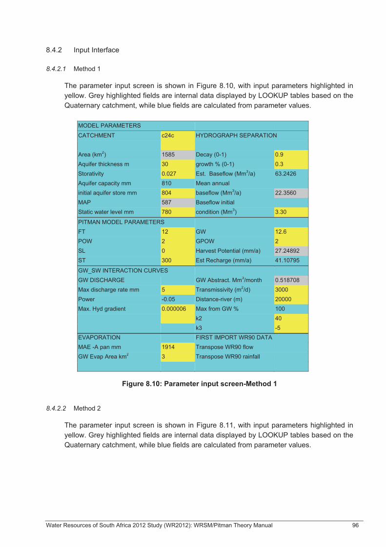
Water Resources of South Africa 2012 Study (WR2012): WRSM/Pitman Theory Manual 96
8.4.2 Input Interface
8.4.2.1 Method 1
The parameter input screen is shown in Figure 8.10, with input parameters highlighted in yellow. Grey highlighted fields are internal data displayed by LOOKUP tables based on the Quaternary catchment, while blue fields are calculated from parameter values.
MODEL PARAMETERS
CATCHMENT c24c HYDROGRAPH SEPARATION Area (km2) 1585 Decay (0-1) 0.9 Aquifer thickness m 30 growth % (0-1) 0.3 Storativity 0.027 Est. Baseflow (Mm3/a) 63.2426 Aquifer capacity mm 810 Mean annual initial aquifer store mm 804 baseflow (Mm3/a) 22.3560 MAP 587 Baseflow initial Static water level mm 780 condition (Mm3) 3.30
PITMAN MODEL PARAMETERS FT 12 GW 12.6 POW 2 GPOW 2 SL 0 Harvest Potential (mm/a) 27.24892 ST 300 Est Recharge (mm/a) 41.10795
GW_SW INTERACTION CURVES GW DISCHARGE GW Abstract. Mm3/month 0.518708 Max discharge rate mm 5 Transmissivity (m2/d) 3000 Power -0.05 Distance-river (m) 20000 Max. Hyd gradient 0.000006 Max from GW % 100 k2 40 k3 -5 EVAPORATION FIRST IMPORT WR90 DATA MAE -A pan mm 1914 Transpose WR90 flow GW Evap Area km2 3 Transpose WR90 rainfall
Figure 8.10: Parameter input screen-Method 1
8.4.2.2 Method 2
The parameter input screen is shown in Figure 8.11, with input parameters highlighted in yellow. Grey highlighted fields are internal data displayed by LOOKUP tables based on the Quaternary catchment, while blue fields are calculated from parameter values.
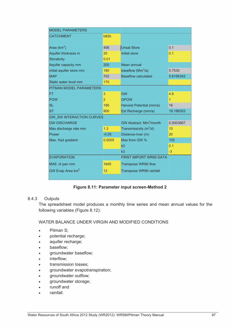
Water Resources of South Africa 2012 Study (WR2012): WRSM/Pitman Theory Manual 97
MODEL PARAMETERS
CATCHMENT b82b Area (km2) 406 Unsat Store 0.1 Aquifer thickness m 20 Initial store 0.1 Storativity 0.01 Aquifer capacity mm 200 Mean annual initial aquifer store mm 180 baseflow (Mm3/a) 5.7530 MAP 702 Baseflow calculated 5.6195342 Static water level mm 170
PITMAN MODEL PARAMETERS FT 3 GW 4.6 POW 2 GPOW 1 SL 190 Harvest Potential (mm/a) 16 ST 800 Est Recharge (mm/a) 19.186303
GW_SW INTERACTION CURVES GW DISCHARGE GW Abstract. Mm3/month 0.0003667 Max discharge rate mm 1.3 Transmissivity (m2/d) 10 Power -0.05 Distance-river (m) 20 Max. Hyd gradient 0.0005 Max from GW % 105 k2 0.1 k3 -3 EVAPORATION FIRST IMPORT WR90 DATA
MAE -A pan mm 1645 Transpose WR90 flow GW Evap Area km2 12 Transpose WR90 rainfall
Figure 8.11: Parameter input screen-Method 2
8.4.3 Outputs The spreadsheet model produces a monthly time series and mean annual values for the following variables (Figure 8.12): WATER BALANCE UNDER VIRGIN AND MODIFIED CONDITIONS
• Pitman S; • potential recharge; • aquifer recharge; • baseflow; • groundwater baseflow; • interflow; • transmission losses; • groundwater evapotranspiration; • groundwater outflow; • groundwater storage; • runoff and • rainfall.

Water Resources of South Africa 2012 Study (WR2012): WRSM/Pitman Theory Manual 98
TIME SERIES GRAPHICS In addition to time series graphics of the above monthly time series, graphs of the following value adding variables are included:
• duration curves of baseflow under modified and virgin conditions; • duration curve of percentage baseflow depletion; • annual rainfall versus recharge; • probability curve of recharge non-exceedance and • return period of drought recharge.
WATER BALANCE MODIFIED 1987-1995
Potential recharge mm 32.60
VIRGIN STATE MAP mm 501.41 MAR mm 39.18 MAR mm 17.11 MAP mm 587.79 Abstraction (Mm3/a) 21.24 Potential Recharge mm/a 41.11 Abstraction (mm/a) 13.40 Aquifer Recharge mm/a 37.79 Aquifer Recharge mm/a 28.98 Baseflow mm/a 39.15 Baseflow mm/a 17.07 G'water B'flow mm/a 36.01 G'water B'flow mm/a 17.07 Interflow mm/a 3.14 Interflow mm/a 0.00 Transmission losses mm/a 0.00 Transmission losses (mm) 0.00 G'Water Evap mm/a 1.38 G'Water Evap mm/a 1.01 G'water outflow mm/a 0.41 G'water outflow mm/a 0.30 Aquifer storage mm -0.5922 Aquifer storage mm -22.58 WATER BALANCE 0.17 WATER BALANCE 0.82
AQUIFER BALANCE -0.01 AQUIFER BALANCE -2.80
Figure 8.12: Water balance display
8.5 Worked example – Middle Letaba B82B
8.5.1 Setup The spreadsheet model was applied to the middle Letaba catchment B82B and other catchments using method 2 in order to determine the impacts of groundwater abstraction on inflows into the Middle Letaba dam. The catchment is underlain by granites and is relatively steep. Baseflow is generated from high lying springs as interflow, and from groundwater in the valley bottoms. The model was run for the period 1922-1996. Irrigation using groundwater began in 1986 and increased from 9.8 to 12.2 Mm3/a. Irrigation was distributed into monthly abstraction volumes using crop water requirements. The MAR is 15.9 Mm3/a. The Pitman model parameters were used to generate the flow sequence and Pitman S values are shown in Table 8.2. Input parameters for the surface-groundwater model are shown in Figure 8.13.
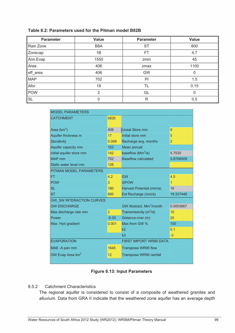
Water Resources of South Africa 2012 Study (WR2012): WRSM/Pitman Theory Manual 99
Table 8.2: Parameters used for the Pitman model B82B
Parameter Value Parameter Value Rain Zone B8A ST 800
Zonevap 1B FT 4.7
Ann.Evap 1550 zmin 45
Area 406 zmax 1100
eff_area 406 GW 0
MAP 702 PI 1.5
Afor 19 TL 0.15
POW 2 GL 0
SL 0 R 0.5
MODEL PARAMETERS
CATCHMENT b82b Area (km2) 406 Unsat Store mm 9 Aquifer thickness m 17 Initial store mm 5 Storativity 0.009 Recharge avg. months 2 Aquifer capacity mm 153 Mean annual initial aquifer store mm 142 baseflow (Mm3/a) 5.7530 MAP mm 702 Baseflow calculated 5.8768009 Static water level mm 126
PITMAN MODEL PARAMETERS FT 4.2 GW 4.5 POW 3 GPOW 1 SL 180 Harvest Potential (mm/a) 16 ST 800 Est Recharge (mm/a) 19.337448
GW_SW INTERACTION CURVES GW DISCHARGE GW Abstract. Mm3/month 0.0003667 Max discharge rate mm 2 Transmissivity (m2/d) 10 Power -0.05 Distance-river (m) 20 Max. Hyd gradient 0.001 Max from GW % 100 k2 0.1 k3 -3 EVAPORATION FIRST IMPORT WR90 DATA
MAE -A pan mm 1645 Transpose WR90 flow GW Evap Area km2 12 Transpose WR90 rainfall
Figure 8.13: Input Parameters
8.5.2 Catchment Characteristics The regional aquifer is considered to consist of a composite of weathered granites and alluvium. Data from GRA II indicate that the weathered zone aquifer has an average depth
Water Resources of South Africa 2012 Study (WR2012): WRSM/Pitman Theory Manual 100
of 34 m and an average specific yield of 0.009. Given an area of 406 km², this would give a volume of 124 Mm³ stored in the weathered zone. However, only 50% of boreholes are successful, indicating 50% of the area has very limited storage. As a result, aquifer storage was taken as 62 Mm³. This is equivalent to a depth of 153 mm. Using this value for aquifer capacity, an average aquifer thickness depth of 17 m was calculated. Water levels generally fluctuate about 3 m seasonally. When multiplied by the specific yield value of 0.009, this indicates that aquifer storage drops an average of 27 mm seasonally. Consequently a static water level of 126 mm was selected. (153 mm – 27 mm). GRA II lists the catchment as having a storativity of 0.00017 for the fractured granite aquifer and 0.009 for the weathered aquifer. The average water level is 21 m deep. Approximately 3% of the catchment consists on valley bottom where a significant weathered zone exists. The remainder of the catchment consists largely of fractured granite. This gives a weighted mean storativity of 0.00043. When multiplied by the average depth to the water level, a volume of 9 mm can be calculated for the unsaturated percolating zone. The length of the moving average of recharge was calculated from the unsaturated percolating store (9 mm), divided by the aquifer recharge listed in GRA II project 3B (22 mm/12 months) times 0.5. This gives a turnover time of 2.5 months. Consequently, a moving average of 2 months was selected. Project 3A lists recharge as 17 mm/a, which would yield a 3 month turnover time for the percolating storage. To calculate groundwater evaporation, monthly rainfall distributions for rainfall zone B8A were imported from WR90 and transformed to monthly rainfalls based on an MAP of 702 mm. A-Pan data was converted from 1550 mm S-pan evaporation listed in WR90. Monthly distribution factors for zone 1B were applied. Crop factors applied were those for Inland Tropical Forest, as listed in WR90. An evaporation area of 12 km² was estimated based on 3% of the catchment area. This approximates the valley bottom area where groundwater is believed to be shallow. Groundwater outflow was calculated based on a transmissivity of 10 m²/d for the weathered zone. A maximum hydraulic gradient (HGRAD) of 0.001 was determined from channel gradients at the base of the catchment. This is the hydraulic gradient applied when groundwater storage is at aquifer capacity.
8.5.3 Baseflow Generation parameters WSAM lists baseflow as being 5.75 Mm³/a, or 14 mm/a, and the Harvest Potential as 16 mm/a. GRA II lists recharge as 17 mm/a (project 3A) or aquifer recharge as 22 mm/a and potential recharge as 24 mm/a. To determine the maximum rate of groundwater baseflow, the hydrograph for the entire period was examined (Figure 8.14). It was assumed that at the end of the dry season (September), all discharge would be from groundwater. In the wettest period (1995),

Water Resources of South Africa 2012 Study (WR2012): WRSM/Pitman Theory Manual 101
discharge was 0.8 Mm³. This equates to a discharge rate of 1.97 mm, consequently a maximum discharge rate at aquifer capacity of 2 mm/month was selected. Parameters FT, POW, GW and GPOW were calibrated to achieve a visual fit of the recession period of the hydrograph. Emphasis was placed on the period 1929-1939 to cover the driest period on record (Figure 8.15) and the period 1969-1996 to cover two wet periods and an intervening dry period (Figure 8.16).
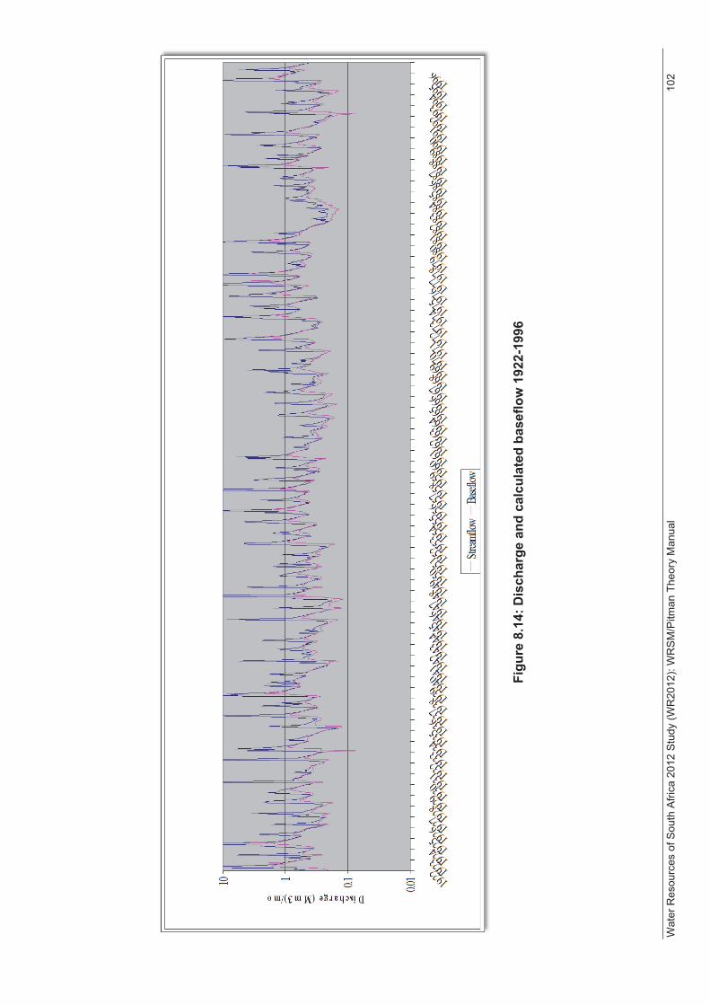
Wat
er R
esou
rces
of S
outh
Afri
ca 2
012
Stu
dy (W
R20
12):
WR
SM
/Pitm
an T
heor
y M
anua
l 1
02
Figu
re 8
.14:
Dis
char
ge a
nd c
alcu
late
d ba
seflo
w 1
922-
1996

Water Resources of South Africa 2012 Study (WR2012): WRSM/Pitman Theory Manual 103
Figure 8.15: Discharge and calculated baseflow 1929-1939
Figure 8.16: Discharge and calculated baseflow 1968-1996
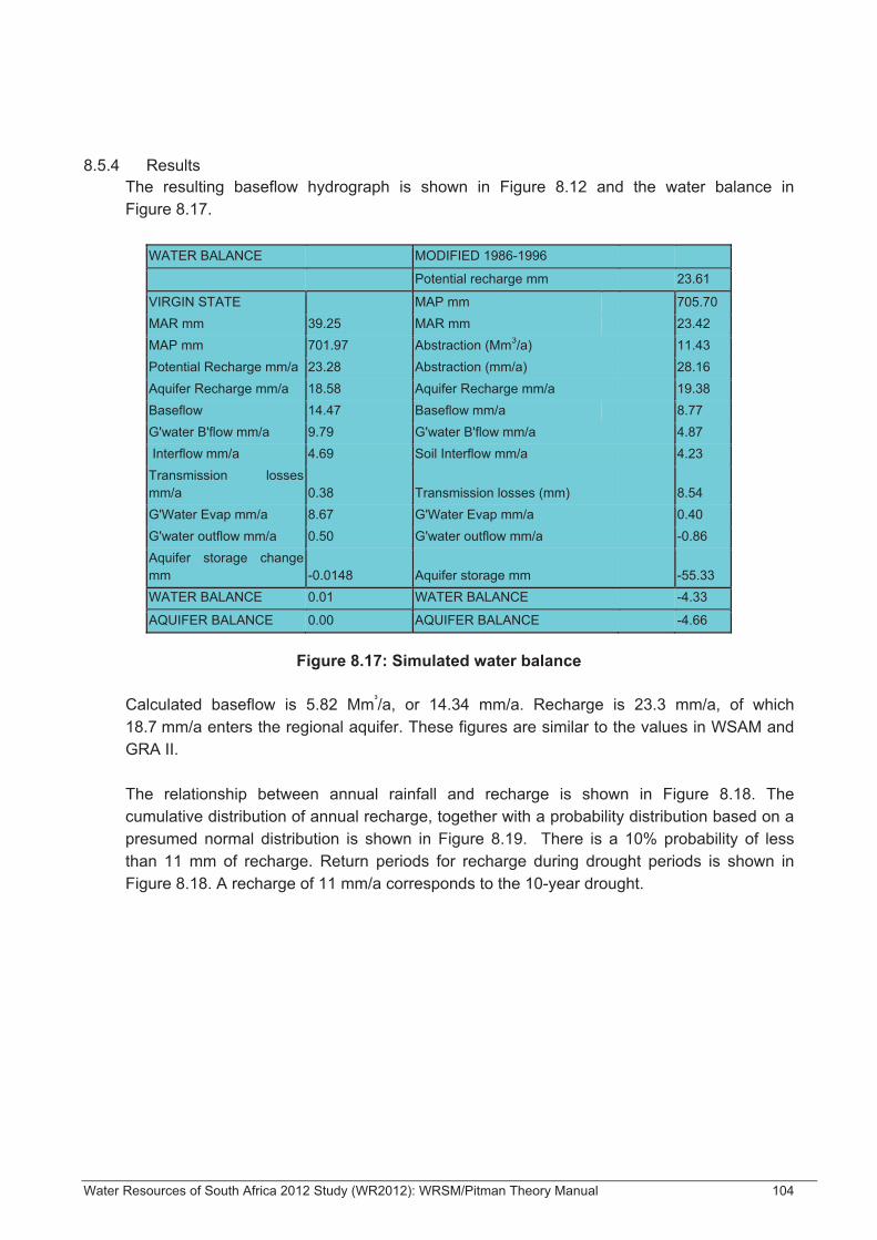
Water Resources of South Africa 2012 Study (WR2012): WRSM/Pitman Theory Manual 104
8.5.4 Results The resulting baseflow hydrograph is shown in Figure 8.12 and the water balance in Figure 8.17.
WATER BALANCE MODIFIED 1986-1996
Potential recharge mm 23.61
VIRGIN STATE MAP mm 705.70 MAR mm 39.25 MAR mm 23.42 MAP mm 701.97 Abstraction (Mm3/a) 11.43 Potential Recharge mm/a 23.28 Abstraction (mm/a) 28.16 Aquifer Recharge mm/a 18.58 Aquifer Recharge mm/a 19.38 Baseflow 14.47 Baseflow mm/a 8.77 G'water B'flow mm/a 9.79 G'water B'flow mm/a 4.87 Interflow mm/a 4.69 Soil Interflow mm/a 4.23 Transmission losses mm/a 0.38 Transmission losses (mm) 8.54 G'Water Evap mm/a 8.67 G'Water Evap mm/a 0.40 G'water outflow mm/a 0.50 G'water outflow mm/a -0.86 Aquifer storage change mm -0.0148 Aquifer storage mm -55.33 WATER BALANCE 0.01 WATER BALANCE -4.33
AQUIFER BALANCE 0.00 AQUIFER BALANCE -4.66
Figure 8.17: Simulated water balance Calculated baseflow is 5.82 Mm³/a, or 14.34 mm/a. Recharge is 23.3 mm/a, of which 18.7 mm/a enters the regional aquifer. These figures are similar to the values in WSAM and GRA II. The relationship between annual rainfall and recharge is shown in Figure 8.18. The cumulative distribution of annual recharge, together with a probability distribution based on a presumed normal distribution is shown in Figure 8.19. There is a 10% probability of less than 11 mm of recharge. Return periods for recharge during drought periods is shown in Figure 8.18. A recharge of 11 mm/a corresponds to the 10-year drought.

Water Resources of South Africa 2012 Study (WR2012): WRSM/Pitman Theory Manual 105
Figure 8.18: Relationship between annual rainfall and recharge
Figure 8.19: Probability distribution of annual recharge
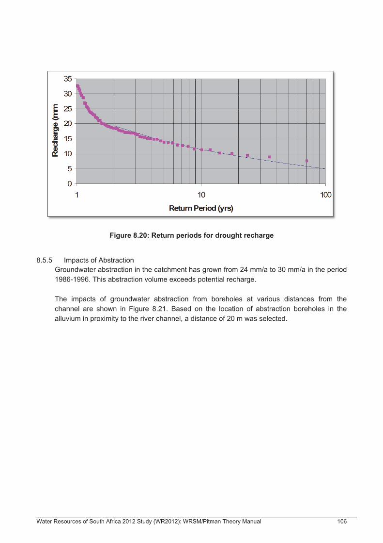
Water Resources of South Africa 2012 Study (WR2012): WRSM/Pitman Theory Manual 106
Figure 8.20: Return periods for drought recharge
8.5.5 Impacts of Abstraction Groundwater abstraction in the catchment has grown from 24 mm/a to 30 mm/a in the period 1986-1996. This abstraction volume exceeds potential recharge. The impacts of groundwater abstraction from boreholes at various distances from the channel are shown in Figure 8.21. Based on the location of abstraction boreholes in the alluvium in proximity to the river channel, a distance of 20 m was selected.
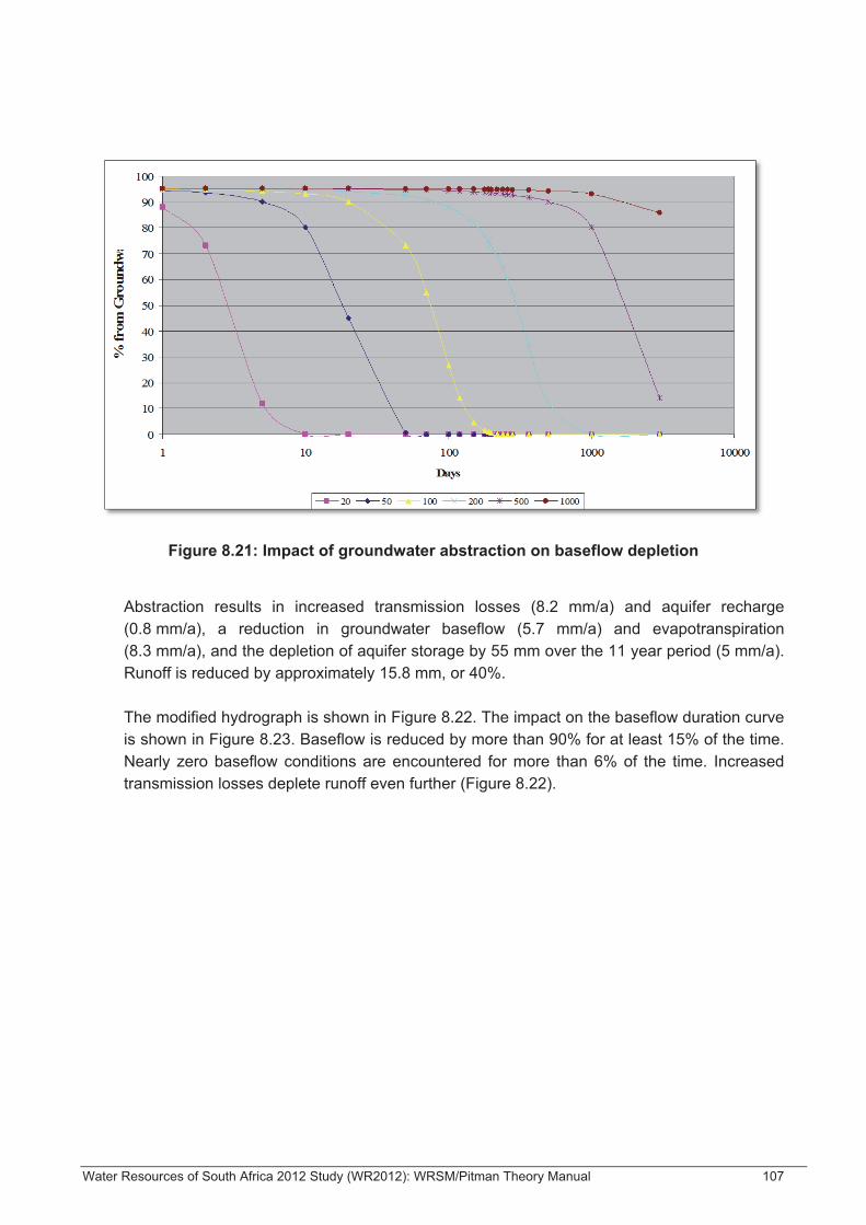
Water Resources of South Africa 2012 Study (WR2012): WRSM/Pitman Theory Manual 107
Figure 8.21: Impact of groundwater abstraction on baseflow depletion
Abstraction results in increased transmission losses (8.2 mm/a) and aquifer recharge (0.8 mm/a), a reduction in groundwater baseflow (5.7 mm/a) and evapotranspiration (8.3 mm/a), and the depletion of aquifer storage by 55 mm over the 11 year period (5 mm/a). Runoff is reduced by approximately 15.8 mm, or 40%. The modified hydrograph is shown in Figure 8.22. The impact on the baseflow duration curve is shown in Figure 8.23. Baseflow is reduced by more than 90% for at least 15% of the time. Nearly zero baseflow conditions are encountered for more than 6% of the time. Increased transmission losses deplete runoff even further (Figure 8.22).
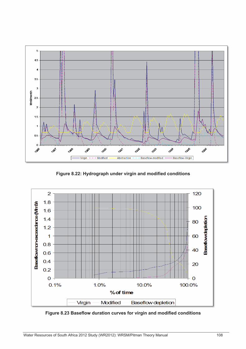
Water Resources of South Africa 2012 Study (WR2012): WRSM/Pitman Theory Manual 108
Figure 8.22: Hydrograph under virgin and modified conditions
Figure 8.23 Baseflow duration curves for virgin and modified conditions
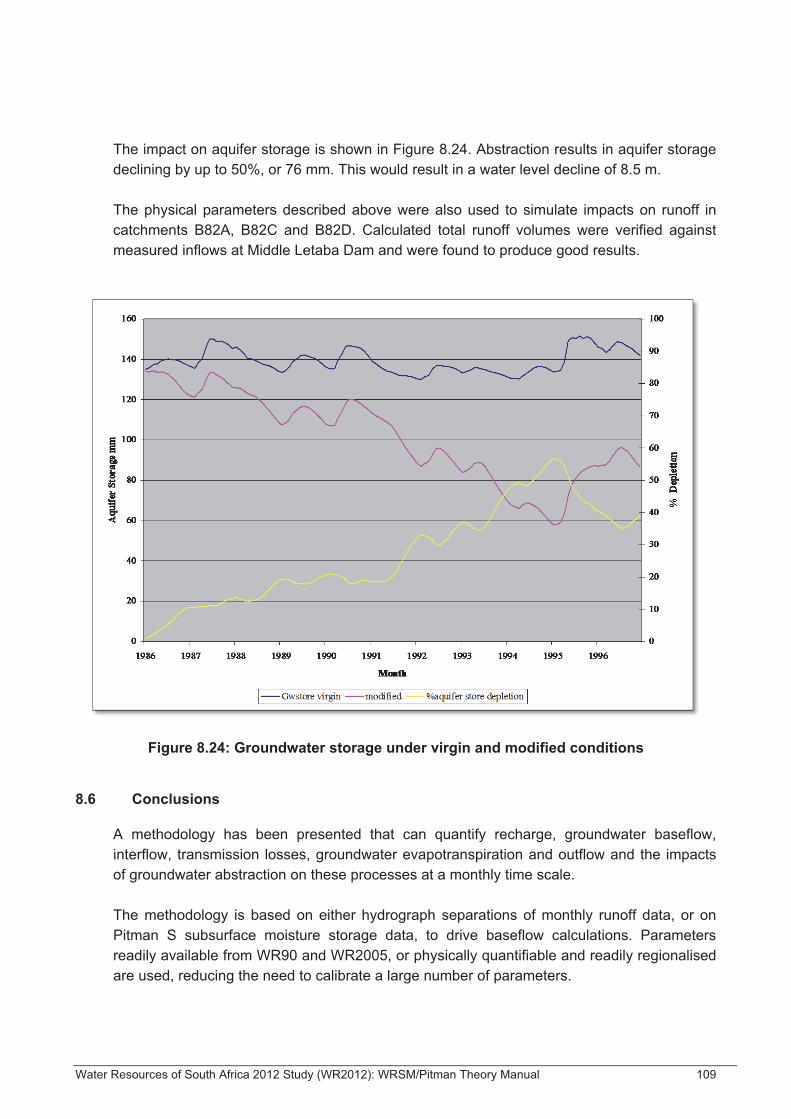
Water Resources of South Africa 2012 Study (WR2012): WRSM/Pitman Theory Manual 109
The impact on aquifer storage is shown in Figure 8.24. Abstraction results in aquifer storage declining by up to 50%, or 76 mm. This would result in a water level decline of 8.5 m. The physical parameters described above were also used to simulate impacts on runoff in catchments B82A, B82C and B82D. Calculated total runoff volumes were verified against measured inflows at Middle Letaba Dam and were found to produce good results.
Figure 8.24: Groundwater storage under virgin and modified conditions
8.6 Conclusions
A methodology has been presented that can quantify recharge, groundwater baseflow, interflow, transmission losses, groundwater evapotranspiration and outflow and the impacts of groundwater abstraction on these processes at a monthly time scale. The methodology is based on either hydrograph separations of monthly runoff data, or on Pitman S subsurface moisture storage data, to drive baseflow calculations. Parameters readily available from WR90 and WR2005, or physically quantifiable and readily regionalised are used, reducing the need to calibrate a large number of parameters.

Water Resources of South Africa 2012 Study (WR2012): WRSM/Pitman Theory Manual 110
The methodology has been incorporated into an MS-EXCEL spreadsheet with graphical facilities to simulate individual Quaternary catchments. Timer series data are calculated and displayed. The spreadsheet contains facilities for time series data analysis of baseflow duration, baseflow depletion, rainfall-recharge relationships, and drought recharge scenarios. The methodology provides a rapid assessment of groundwater surface water interactions and the potential impacts of abstraction using basic data available primarily within WR90, with a minimum of intuitive parameters. Current shortcomings with application of the methodology are as follows:
• uncertainty as to actual baseflow figures against which to calibrate calculated baseflow volumes;
• uncertainty and lack of recharge figures to calibrate GW and GPOW and
• arbitrary nature of K2 and k3 parameters controlling the relationship between abstraction and baseflow depletion due to lack of data regarding impacts of abstraction against which to calibrate these parameters.
Currently, no data is available to calibrate the algorithm of groundwater abstraction impacts on baseflow depletion. It is uncertain the degree to which distance from the borehole impacts on baseflow under transient conditions. For this reason, the parameters k2 and k3, which control the timing and rate of the transition between depletion of groundwater storage and baseflow depletion under fixed transmissivity and distance conditions, cannot be rigorously verified. If case studies based on long duration test pumping in the field could be obtained and calibrated, these parameters could possibly be fixed within the algorithm and removed, with only the catchment parameters of transmissivity and distance being used to control the impacts of abstraction.
8.7 References
ACT 108, 1997. Republic of South Africa Water Services Act. Hughes, DA (2004). Incorporating groundwater recharge and discharge functions into an existing monthly rainfall-runoff model. Hyd. Sci J. (in press). Sophocleous, Marios, 2002. Interactions between groundwater and Surface water: the state of the science. Hydrogeology J. 10:52-67. Vegter, J.R., 1996. Recharge and streamflow. Workshop on groundwater-surface water issues in arid and semi-arid areas, Water Research Commission. Vegter, J.R. (2001). Groundwater Development In South Africa. WRC Report No. TT134/00, Pretoria, South Africa.

Water Resources of South Africa 2012 Study (WR2012): WRSM/Pitman Theory Manual 111
8.8 Glossary
Table 8.3: Glossary
Term Definition
Groundwater baseflow Baseflow from the regional aquifer resulting from the water table being above river stage. This is water that could potentially be impacted upon by pumping from the aquifer
Harvest Potential The maximum that can be abstracted per unit area based on recharge, transmissivity and aquifer storage constraints
Interflow
Baseflow from a combination of subsurface pathways, including baseflow from sources not in contact with the regional aquifer due to geological boundary conditions, baseflow from soil moisture, potential recharge that cannot percolate downwards due to saturated conditions (aquifer at capacity)
Potential recharge Recharge that could reach the aquifer if the aquifer is not at capacity. This recharge includes recharge supplying baseflow for springs or perched aquifers, hence not all recharge is available to the regional aquifer
Aquifer recharge Recharge reaching the regional aquifer and supplying groundwater baseflow, evapotranspiration, abstraction and outflow
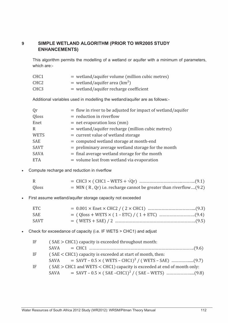
Water Resources of South Africa 2012 Study (WR2012): WRSM/Pitman Theory Manual 112
9 SIMPLE WETLAND ALGORITHM (PRIOR TO WR2005 STUDY ENHANCEMENTS)
This algorithm permits the modelling of a wetland or aquifer with a minimum of parameters, which are:-
Additional variables used in modelling the wetland/aquifer are as follows:-
• Compute recharge and reduction in riverflow
√
• First assume wetland/aquifer storage capacity not exceeded
• Check for exceedance of capacity (i.e. IF WETS > CHC1) and adjust
Water Resources of South Africa 2012 Study (WR2012): WRSM/Pitman Theory Manual 113
If none of the above conditions apply, capacity is never exceeded:
• Adjust water balance for the month and reduce riverflow accordingly
Water Resources of South Africa 2012 Study (WR2012): WRSM/Pitman Theory Manual 114
10 COMPREHENSIVE WETLAND SUB-MODEL INCLUDING OFF-CHANNEL STORAGE (WITH WR2005 STUDY ENHANCEMENTS) BY DR WV PITMAN
10.1 Description of Old Wetland Sub-model plus reasons for improvement
The old wetland model comprises an in-channel storage with a nominal storage volume and surface area, which can be exceeded during high flows. It works very much like a reservoir where downstream flow takes place only when the (nominal) storage capacity of the wetland is exceeded. This configuration is not realistic for wetlands comprising a defined channel that meanders through a wetland, feeding it with water only when the river channel capacity is exceeded. The flow of water between channel and wetland can be in the form of overbank spillage or via channels, or a combination of both. Examples of such wetlands are to be found in the Kafue River (Zambia) and the Pongolo River (RSA). The new wetland model described below is designed to simulate a wetland that is either off-channel or in-channel. It can also be employed to simulate the effect of a man-made off-channel storage dam for water supply.
10.2 Description of New Wetland Sub-model
The new wetland model is depicted in the diagram in Figure 10.1 below. (Showing a single link from river channel to wetland and another single link from wetland back into the channel facilitates visualization of the model. A real wetland has many links, where water can flow from channel to wetland and from wetland back into the channel, depending on water levels.) As is the case for the old model, the wetland has a nominal storage capacity and surface area, which can be exceeded. In the new model, however, the nominal values refer to the wetland storage (and associated area) below which there is no linkage to the river channel. Flow from wetland to channel is governed by the storage state of the wetland and is proportional to the storage volume over and above the nominal capacity. Flow from channel to wetland occurs when channel flow is above a prescribed threshold. The surplus flow is then apportioned between river channel and wetland link. If the model is to be used to simulate off-channel storage an upper limit can be set for the flow in the channel to wetland link, equivalent to the diversion capacity. The model also caters for local runoff entering directly into the wetland. This wetlands model links only to surface water flow and does not include groundwater fed wetlands. A description of the various algorithms used to model the wetland follows. Units of million cubic metres (10 m³) are used throughout for volumes and flow rates are in million cubic metres per month.
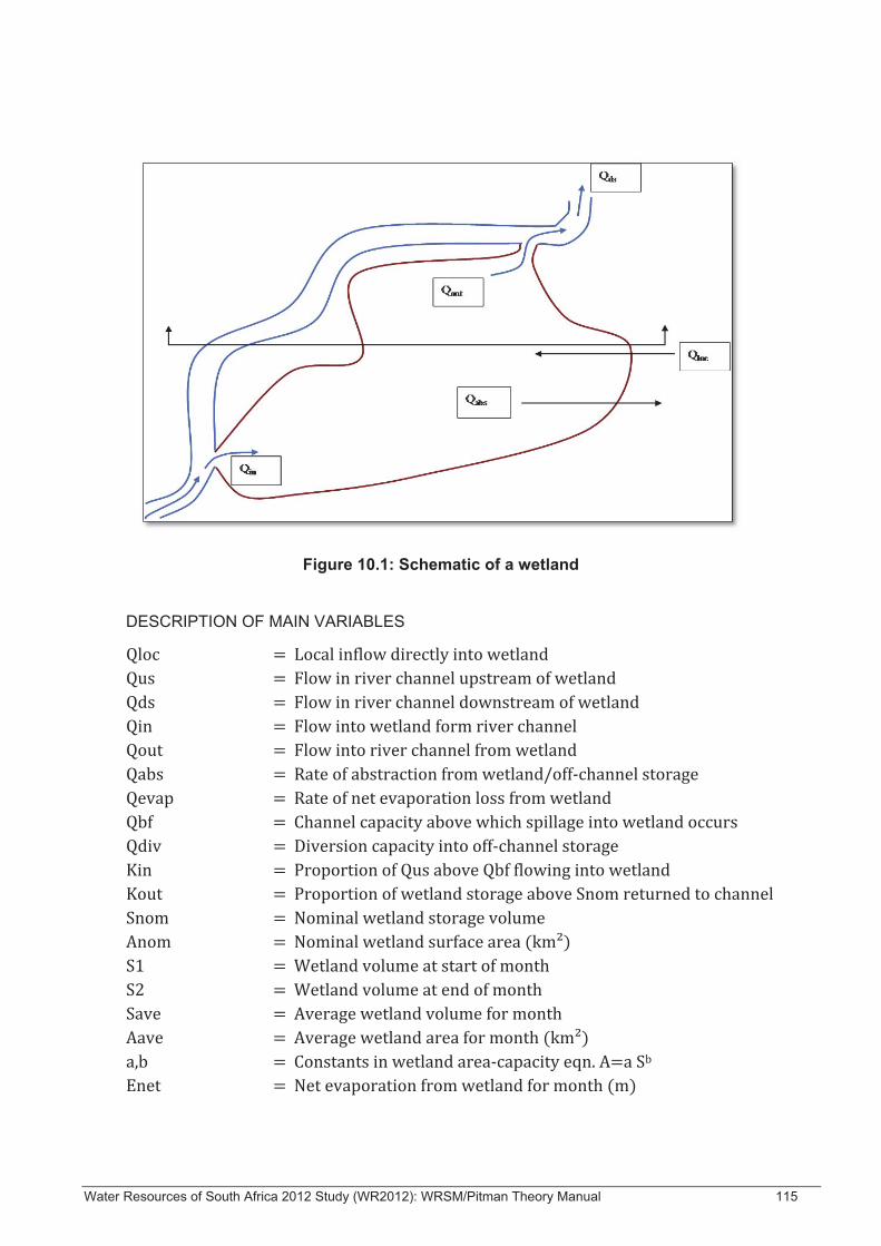
Water Resources of South Africa 2012 Study (WR2012): WRSM/Pitman Theory Manual 115
Figure 10.1: Schematic of a wetland
DESCRIPTION OF MAIN VARIABLES

Water Resources of South Africa 2012 Study (WR2012): WRSM/Pitman Theory Manual 116
10.3 Water balance for wetland
Inflow to the wetland is from the river channel, whereas outflow can be a combination of flow back into the channel, net evaporation loss and abstractions from the wetland (or off-channel storage). In times of heavy rain the net evaporation rate can be negative and constitute an additional input to the wetland.
10.4 Flow into wetland
If flow in the channel is less than the threshold value Qbf, then there is no inflow. Above the threshold the inflow is a proportion of the channel flow above Qbf. If an off-channel scheme is being modelled, Qbf becomes the flow below which no diversion is allowed (say, for the Reserve) and Qdiv is the maximum rate of transfer to the off-channel dam, viz. the diversion capacity. For a natural wetland Qdiv is not used, hence an arbitrary large value is assigned in the model. An in-channel wetland can be modelled by setting Qbf equal to zero and Kin equal to 1, such that all flow enters the wetland.
10.5 Outflow from wetland
Outflow from the wetland back into the channel occurs only when the wetland volume exceeds the nominal storage. The factor Kout determines the rate at which the surplus water drains back to the channel. For some very extensive wetlands a low value of Kout would be appropriate, signifying a slow release of water back to the channel. However, if an off-channel scheme is being modelled the value of Kout would be close to unity, since the dam would be provided with a spillway.
10.6 Evaporation from wetland
The net evaporation loss Enet is determined in the usual manner by subtracting rainfall from the gross evaporation, which is derived by applying a coefficient to the monthly pan evaporation. The relationship between wetland volume and surface area is given by the equation A = aSb, where a and b are constants defined by the shape of the wetland basin. For most wetlands one has a good estimate of the nominal surface area (Anom) and the nominal volume (Snom) can be estimated by assuming an average water depth. The coefficient b can be derived by assuming a basin shape: a typical value for b is plus/minus 0.5. The value of a can then be determined by the following equation.

Water Resources of South Africa 2012 Study (WR2012): WRSM/Pitman Theory Manual 117
The net evaporation can now be calculated from the wetland storage state as follows:
10.7 Flow downstream of wetland
The flow downstream of the wetland is simply the upstream flow less inflow to the wetland plus outflow back to the river channel. For most months Qds will be less than Qus (i.e. Qin > Qout). However, periods immediately after high flow can be followed by a net increase in flow as floodwater drains back into the river channel.
10.7.1 Notes on Solution of Water Balance Owing to the coarse time step (one month) it is necessary to perform some kind of iteration to achieve a water balance of sufficient accuracy. The model achieves this by making successive approximations to the average wetland storage (Save) until the difference between successive estimates is less than a predetermined value.
10.8 Preliminary Testing of New Wetland Model using the Kafue wetland
Hydrological modelling of the upper Kafue basin, which contains an extensive wetland, has been undertaken recently. It was during the course of this study that the shortcomings of existing wetland model (in WRSM/Pitman) were exposed, in that it was necessary to reduce dry season flows to zero in order to achieve the correct evaporative losses from the wetland. A stand-alone computer program (called SWAMP2) has been written for the purposes of development and testing. (Please note that variable names in the program are not necessarily the same as used in the preceding model description.)
10.8.1 Data inputs The basic data required by the program is listed and described below. Line1: 900 2500 2500 0.5 400 0.25 0.25 Line 2: 0.0 0.0 Line 3: 180 175 180 175 150 140 115 100 85 85 115 160 Line 4: 1969 1990 Line 5: 'kafue.ran' Line 6: '4350.obs' Line 7: ‘K2RQ58.ANS' Line 1 contains the model parameters that need to be adjusted in the calibration process.

Water Resources of South Africa 2012 Study (WR2012): WRSM/Pitman Theory Manual 118
(The exception is the first variable, which can be obtained from rainfall information.) Some indication of the wetland area can usually be obtained from suitable mapping. 900 Mean annual precipitation on wetland (see description of Line 5) 2500 Nominal wetland surface area Nominal wetland volume Power coefficient of wetland area-volume equation River channel capacity Proportion of river flow (above capacity) flowing into wetland Proportion of wetland volume (above nominal capacity) flowing back to river Line 2 contains two variables for modelling an off-channel storage scheme, as follows: Maximum diversion capacity (set to 0.0 if not applicable) Rate of abstraction from wetland/off-channel storage Line 3 contains the 12 mean monthly evaporations applicable to wetland (Oct to Sep) Line 4 contains the first and last years of the period to be simulated Line 5 contains the rainfall filename. Note that it is a file of monthly rainfalls as percentages of MAP, which gets converted to mm in the program. Line 6 contains the file of monthly river flow upstream of the wetland. Line 7 contains the file of local monthly flows that flow directly into the wetland. If there are no such flows then a blank filename (‘ ‘) is entered.
10.8.2 Model results The model was calibrated on the flow record at a gauge downstream of the wetland. No attempt was made to “fine tune” the calibration – the main purpose of the exercise was to ascertain whether the model could simulate adequately the effect of the wetland on flows downstream of it. The diagram on the top of the following page contains observed mean monthly flows upstream and downstream of the wetland, as well as the simulated downstream values. It shows how the model has reproduced the truncation of the high flows whilst leaving the low flows virtually unaffected.
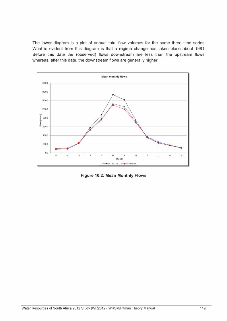
Water Resources of South Africa 2012 Study (WR2012): WRSM/Pitman Theory Manual 119
The lower diagram is a plot of annual total flow volumes for the same three time series. What is evident from this diagram is that a regime change has taken place about 1981. Before this date the (observed) flows downstream are less than the upstream flows, whereas, after this date, the downstream flows are generally higher.
Figure 10.2: Mean Monthly Flows
0.0
200.0
400.0
600.0
800.0
1000.0
1200.0
1400.0
1600.0
O N D J F M A M J J A S
Flow
(mcm
)
Month
Mean monthly flows
Obs u/s Obs d/s
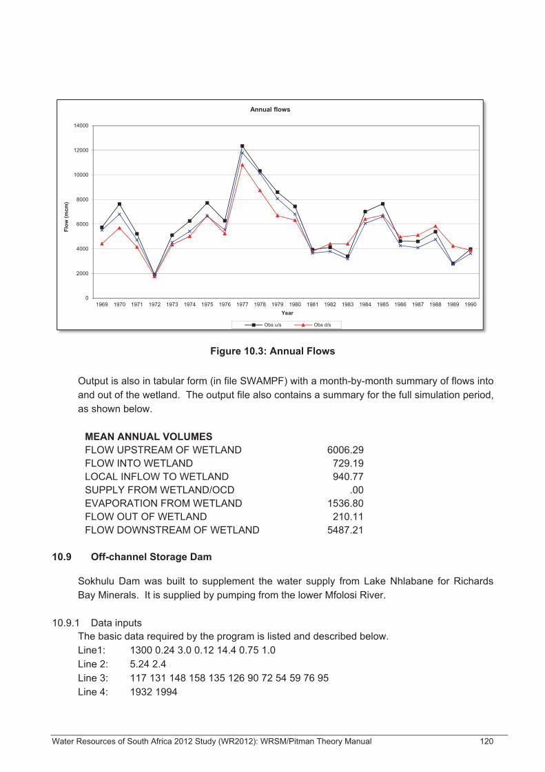
Water Resources of South Africa 2012 Study (WR2012): WRSM/Pitman Theory Manual 120
Figure 10.3: Annual Flows
Output is also in tabular form (in file SWAMPF) with a month-by-month summary of flows into and out of the wetland. The output file also contains a summary for the full simulation period, as shown below.
MEAN ANNUAL VOLUMES FLOW UPSTREAM OF WETLAND 6006.29 FLOW INTO WETLAND 729.19 LOCAL INFLOW TO WETLAND 940.77 SUPPLY FROM WETLAND/OCD .00 EVAPORATION FROM WETLAND 1536.80 FLOW OUT OF WETLAND 210.11 FLOW DOWNSTREAM OF WETLAND 5487.21
10.9 Off-channel Storage Dam
Sokhulu Dam was built to supplement the water supply from Lake Nhlabane for Richards Bay Minerals. It is supplied by pumping from the lower Mfolosi River.
10.9.1 Data inputs The basic data required by the program is listed and described below. Line1: 1300 0.24 3.0 0.12 14.4 0.75 1.0 Line 2: 5.24 2.4 Line 3: 117 131 148 158 135 126 90 72 54 59 76 95 Line 4: 1932 1994
0
2000
4000
6000
8000
10000
12000
14000
1969 1970 1971 1972 1973 1974 1975 1976 1977 1978 1979 1980 1981 1982 1983 1984 1985 1986 1987 1988 1989 1990
Flow
(mcm
)
Year
Annual flows
Obs u/s Obs d/s
Water Resources of South Africa 2012 Study (WR2012): WRSM/Pitman Theory Manual 121
Line 5: ‘kwamb.mp’ Line 6: 'trig52q’ Line 7: ‘ ' Lines 1 and 2 contain the parameters that are required to simulate an off-channel storage scheme, as follows. They are the same as used to model a wetland but some have slightly different interpretations. 1300 Mean annual precipitation on storage dam (see description of Line 5) 0.24 Surface area of storage dam 3.0 Capacity of storage dam 0.12 Power coefficient of area-volume equation for off-channel dam 14.4 Flow in river below which no diversion takes place 0.75 Proportion of river flow (above threshold) diverted to storage dam 1.0 Proportion of dam volume (above capacity) flowing back to river Line 2 contains two variables for modelling an off-channel storage scheme, as follows: 5.24 Maximum diversion capacity (set to 0.0 if not applicable) 2.4 Rate of abstraction from wetland/off-channel storage Line 3 contains the 12 mean monthly evaporations applicable to storage dam (Oct to Sep) Line 4 contains the first and last years of the period to be simulated Line 5 contains the rainfall filename. Note that it is a file of monthly rainfalls as percentages of MAP, which gets converted to mm in the program. Line 6 contains the file of monthly river flow at the diversion point. Line 7 contains the file of local monthly flows that flow directly into the off-channel dam. If there are no such flows then a blank filename (‘ ‘) is entered.
10.9.2 Model results As is the case for the wetland, the model produces an output file with a month-by-month summary and a water balance for the full simulation period, as shown below.
MEAN ANNUAL VOLUMES FLOW UPSTREAM OF WETLAND 864.47 FLOW INTO WETLAND 42.35 LOCAL INFLOW TO WETLAND .00 SUPPLY FROM WETLAND/OCD 3.14 EVAPORATION FROM WETLAND -0.02 FLOW OUT OF WETLAND 9.28 FLOW DOWNSTREAM OF WETLAND 841.41
It is important to note that the diversion into the off-channel dam is not stopped when it reaches full capacity. This may be the case when the dam is fed by a diversion canal, but it would not be true for a pumping scheme. The water balance downstream of the off-channel scheme is, however, correct as all surplus water is immediately spilled back into the river.
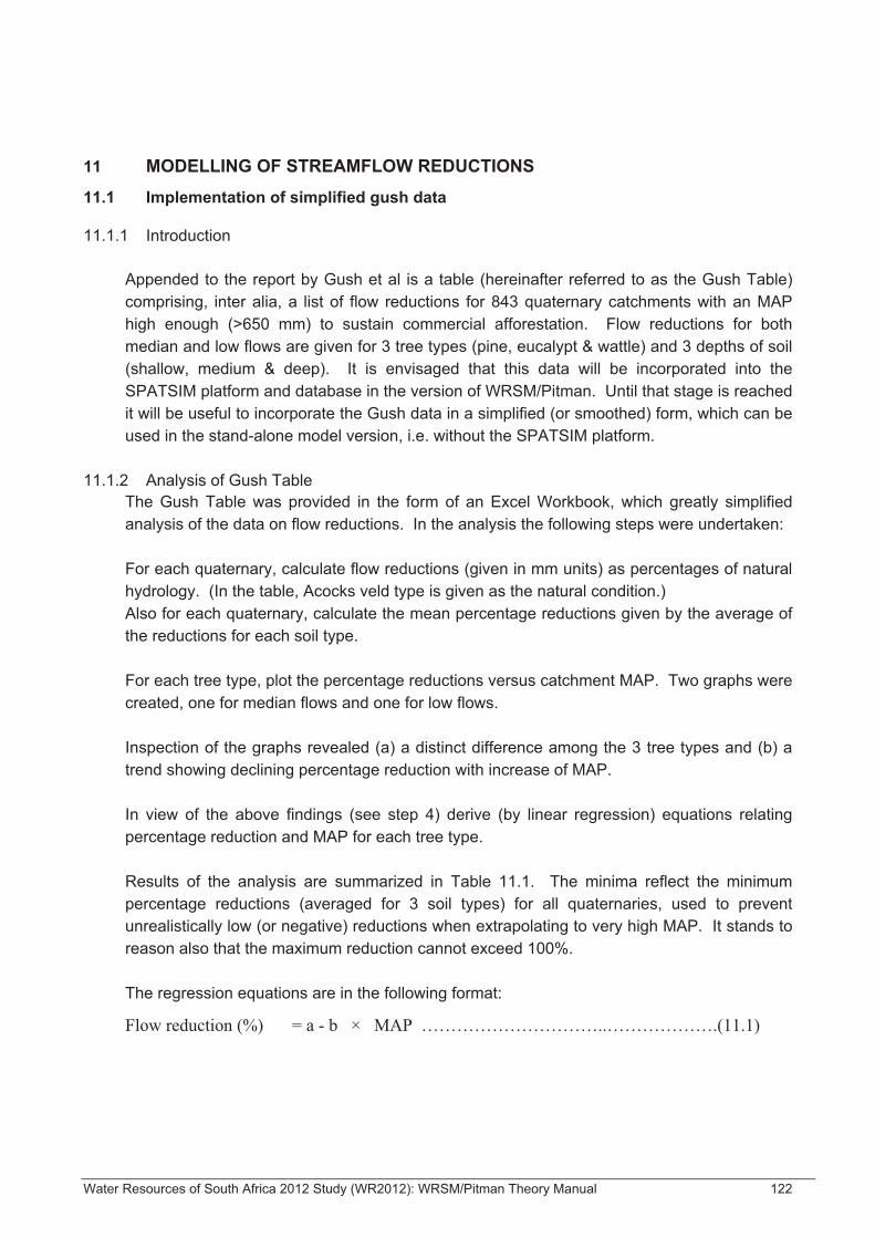
Water Resources of South Africa 2012 Study (WR2012): WRSM/Pitman Theory Manual 122
11 MODELLING OF STREAMFLOW REDUCTIONS 11.1 Implementation of simplified gush data
11.1.1 Introduction
Appended to the report by Gush et al is a table (hereinafter referred to as the Gush Table) comprising, inter alia, a list of flow reductions for 843 quaternary catchments with an MAP high enough (>650 mm) to sustain commercial afforestation. Flow reductions for both median and low flows are given for 3 tree types (pine, eucalypt & wattle) and 3 depths of soil (shallow, medium & deep). It is envisaged that this data will be incorporated into the SPATSIM platform and database in the version of WRSM/Pitman. Until that stage is reached it will be useful to incorporate the Gush data in a simplified (or smoothed) form, which can be used in the stand-alone model version, i.e. without the SPATSIM platform.
11.1.2 Analysis of Gush Table The Gush Table was provided in the form of an Excel Workbook, which greatly simplified analysis of the data on flow reductions. In the analysis the following steps were undertaken: For each quaternary, calculate flow reductions (given in mm units) as percentages of natural hydrology. (In the table, Acocks veld type is given as the natural condition.) Also for each quaternary, calculate the mean percentage reductions given by the average of the reductions for each soil type. For each tree type, plot the percentage reductions versus catchment MAP. Two graphs were created, one for median flows and one for low flows. Inspection of the graphs revealed (a) a distinct difference among the 3 tree types and (b) a trend showing declining percentage reduction with increase of MAP. In view of the above findings (see step 4) derive (by linear regression) equations relating percentage reduction and MAP for each tree type. Results of the analysis are summarized in Table 11.1. The minima reflect the minimum percentage reductions (averaged for 3 soil types) for all quaternaries, used to prevent unrealistically low (or negative) reductions when extrapolating to very high MAP. It stands to reason also that the maximum reduction cannot exceed 100%. The regression equations are in the following format:
Flow reduction (%) = a - b × MAP …………………………..……………….(11.1)
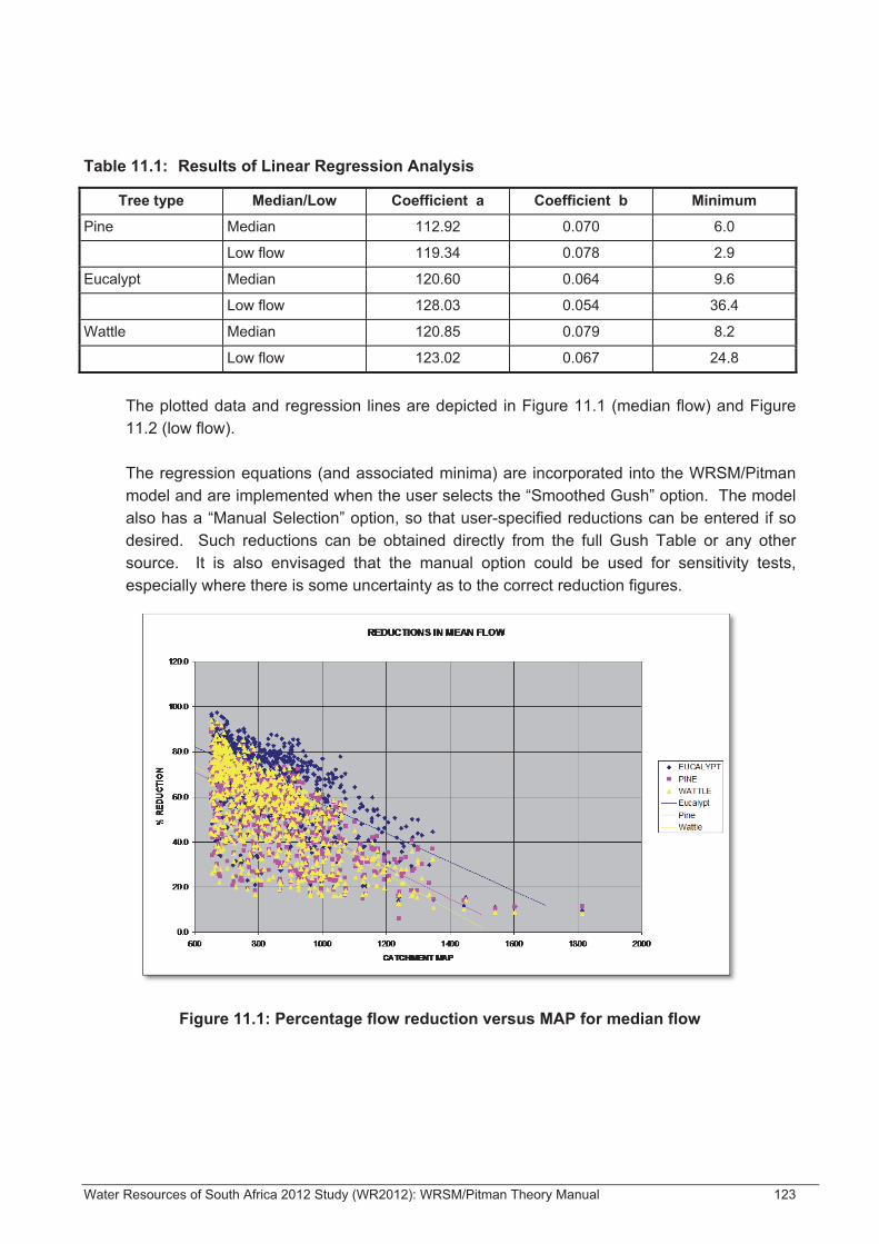
Water Resources of South Africa 2012 Study (WR2012): WRSM/Pitman Theory Manual 123
Table 11.1: Results of Linear Regression Analysis
Tree type Median/Low Coefficient a Coefficient b Minimum
Pine Median 112.92 0.070 6.0
Low flow 119.34 0.078 2.9
Eucalypt Median 120.60 0.064 9.6
Low flow 128.03 0.054 36.4
Wattle Median 120.85 0.079 8.2
Low flow 123.02 0.067 24.8
The plotted data and regression lines are depicted in Figure 11.1 (median flow) and Figure 11.2 (low flow). The regression equations (and associated minima) are incorporated into the WRSM/Pitman model and are implemented when the user selects the “Smoothed Gush” option. The model also has a “Manual Selection” option, so that user-specified reductions can be entered if so desired. Such reductions can be obtained directly from the full Gush Table or any other source. It is also envisaged that the manual option could be used for sensitivity tests, especially where there is some uncertainty as to the correct reduction figures.
Figure 11.1: Percentage flow reduction versus MAP for median flow
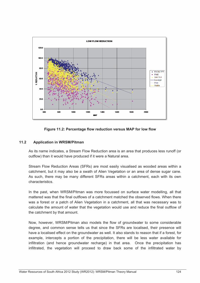
Water Resources of South Africa 2012 Study (WR2012): WRSM/Pitman Theory Manual 124
Figure 11.2: Percentage flow reduction versus MAP for low flow
11.2 Application in WRSM/Pitman
As its name indicates, a Stream Flow Reduction area is an area that produces less runoff (or outflow) than it would have produced if it were a Natural area. Stream Flow Reduction Areas (SFRs) are most easily visualised as wooded areas within a catchment, but it may also be a swath of Alien Vegetation or an area of dense sugar cane. As such, there may be many different SFRs areas within a catchment, each with its own characteristics. In the past, when WRSM/Pitman was more focussed on surface water modelling, all that mattered was that the final outflows of a catchment matched the observed flows. When there was a forest or a patch of Alien Vegetation in a catchment, all that was necessary was to calculate the amount of water that the vegetation would use and reduce the final outflow of the catchment by that amount. Now, however, WRSM/Pitman also models the flow of groundwater to some considerable degree, and common sense tells us that since the SFRs are localised, their presence will have a localised effect on the groundwater as well. It also stands to reason that if a forest, for example, intercepts a portion of the precipitation, there will be less water available for infiltration (and hence groundwater recharge) in that area. Once the precipitation has infiltrated, the vegetation will proceed to draw back some of the infiltrated water by

Water Resources of South Africa 2012 Study (WR2012): WRSM/Pitman Theory Manual 125
evapotranspiration, which will affect the recharge to- and outflow from groundwater, which then affects the final outflow of the wooded area. In the past, therefore, WRSM/Pitman only had one type of catchment: the 'Normal' or 'Free' catchment. A 'Free catchment' is independent of other catchments. A 'Free catchment' has no influence on any other catchment and cannot be influenced by any other catchment either. In order to model the localised effects of SFRs, we have come up with the concept of an 'encompassing catchment' (e.g. the total quaternary catchment) within which smaller 'SFR sub-catchments' take up space, produce less runoff than under natural conditions and so reduce the total runoff of the 'encompassing catchment'. Because they are part of the 'encompassing catchment', the SFR sub-catchments share most (but not all) of the model parameters with the 'encompassing catchment' in which they lie. Conversely, the area of the 'encompassing catchment' would grow and shrink as the areas of the 'SFR sub-catchments' within its borders grow and shrink, to maintain a constant area for the catchment as a whole. To show that an 'encompassing catchment' is in charge – at least as far as simulation parameters are concerned – we decided to call such a catchment a 'Parent catchment'. Since all 'SFR sub-catchments' within a Parent catchment are subordinate to that Parent catchments, we decided to call an 'SFR sub-catchment' a 'Child catchment'. If a catchment is neither a Parent nor a Child, we call this catchment a 'Free catchment' The Parent and Child nomenclature describes the way in which the catchment types act, react and interact with one another very well, and should therefore be taken with a pinch of humour. The following rules apply to the three types of runoff module or catchment: 1. All catchments are created as 'Free' catchments. A Free catchment is neither a Parent nor a Child. A Free catchment has the potential to become either a Parent or a Child. 2. Any Free catchment can be 'elevated' to the status of Parent catchment. A Parent catchment can capture Child catchments to become part of itself. A Parent catchment can free any Child catchment that it does not need any more A Parent catchment cannot be captured by another Parent catchment.
3. A Parent catchment can be told to 'capture' a Free catchment as a Child:

Water Resources of South Africa 2012 Study (WR2012): WRSM/Pitman Theory Manual 126
A Child cannot be captured by more than one Parent. A Child takes on parameters of its Parent only. A Child only runs when told to do so by its Parent. A Child contributes its Runoff to the outflow of the Parent. When freed by its Parent, a Child reverts to a 'Free' catchment.
4. A Parent catchment can be changed to a 'Free' catchment only once it has freed all its
Children. Although, for now, our Child catchments only deal with SFRs areas, this concept could be broadened later to cover Stream Flow Enhancing areas (such as paved areas) as well, since these areas, too, have an influence on groundwater. So far, WRSM/Pitman has been programmed to create Child catchments (i.e. runoff modules) to handle SFRs due to afforestation and alien vegetation. The method used to determine the impact on the hydrological cycle is by the adjustment of certain model parameters, as follows. • PI – the interception storage in mm; • FF – the factor by which potential evapotranspiration is increased; • SL – the soil moisture storage below which runoff ceases and • ST – the total soil moisture capacity. Adjustment of these parameters is done to reflect the following changes wrought by the introduction of forests or alien vegetation : • increased interception due to greater leaf area, etc.; • deeper penetration of tree roots and • increased evapotranspiration (analogous to crop factor effect). Reductions in runoff are generally expressed as percentage reductions in mean (i.e. MAR) and low flows, the latter being the average flows in the lowest quartile. Information obtained from tests on a selection of catchments covering a wide range of climates was used to determine the following relationships between flow reductions and parameter adjustments:
Δ Δ ΔΔ Δ Δ
In order to enable solution of the above equations a predetermined relationship between ΔPI and ΔFF was assumed and it was also assumed that ΔSL and ΔST were the same. The constants A,B,C and X,Y,Z are different for each catchment and depend on MAP and ST. As the above equations do not give an exact result they are used to perform a number of iterations until the closing error is within acceptable limits.

Water Resources of South Africa 2012 Study (WR2012): WRSM/Pitman Theory Manual 127
IMPORTANT NOTE The equations relating flow reductions to changes in model parameters were derived from analyses of catchments suitable for afforestation. Such catchments are located in the wetter parts of South Africa, where the model parameter FT is greater than zero. If FT is zero the equations definitely do not apply. In the (very unlikely) situation of afforestation in a catchment with zero FT one should never try to model the SFR using a Child catchment. The same applies to catchments with alien vegetation. However, as it is more likely for alien vegetation to spread to relatively dry areas where zero values of FT are appropriate. In such cases it will also be necessary to model the impacts on streamflow without a Child module. This should not present any serious problem as, in such catchments, the baseflow proportion of total flow (as derived from groundwater) is usually negligible. In both the above cases, the user cannot obtain either groundwater plots or groundwater time series output because the model does not differentiate between surface and groundwater flow when subtracting the flow due to afforestation and/or alien vegetation. If the user attempts to obtain either, the outputs (plot and/or time series) will be zero.

Water Resources of South Africa 2012 Study (WR2012): WRSM/Pitman Theory Manual 128
12 ALIEN VEGETATION (WR2005 STUDY) INVASIVE ALIEN VEGETATION AND DAM YIELDS – ILLUSTRATING THE IMPACT OF CLEARING PROGRAMMES ON ASSURANCE OF SUPPLY BY DR D LE MAITTRE
Authors: David Le Maitre¹ and André Görgens²·³. With contributions from Mandla Mehlomakulu¹, Johan van Rensburg², Arthur Chapman¹, Dave Scott¹ and Brian van Wilgen¹. The following chapters were extracted from the above report: Chapter 3 Methodology up to section 3.3 (inclusive).
12.1 Methodology
The methodology employed in this study comprised six stages:
• quantifying current levels of infestation;
• projecting future (10 years) levels of infestation;
• formulating a suitable proportional streamflow reduction model for each selected catchment system;
• estimating the respective streamflow sequences for natural, current-level invaded and future-level invaded scenarios via catchment modelling, linked to the streamflow reduction models;
• determining the yields at a range of assurance levels deliverable from a range of hypothetical impoundment sizes for each invasion scenario via reservoir water balance modelling and
• determining the incremental reductions in yields, from natural, for the range of cases analysed.
In the interests of clarity (and economy of effort), it was necessary to ignore all existing human-derived impacts in the selected catchments. In this way, the estimated streamflow reductions due to alien plants could be clearly illustrated, not confounded with the effects of other physical developments on the streamflow regimes of catchments. All alien plant-related impacts were therefore juxtaposed with naturalised streamflows. The generation of these natural streamflows and of the impacts is explained in Section 19.4 below.
12.2 Mapping of Alien Plant Invasions
The data on the extent, density and composition of alien plant invasions was extracted from the databases prepared for each of the management plans. The mapping methods differed between the catchments and this is described below
Water Resources of South Africa 2012 Study (WR2012): WRSM/Pitman Theory Manual 129
Sonderend The catchment was mapped by fieldworkers onto standard 1:50 000 base maps following the procedures and standards set up by Le Maitre and Versfeld (1994) and the data standards developed for the Working for Water Programme (Muller et al. 1999). The species composition was recorded as the percentage canopy cover class for each species. Each mapped area was identified as riparian or non-riparian except in the catchment above the Theewaterskloof Dam where the riparian polygons were not distinguished. The area of the riparian invasions in this portion of the catchment was estimated from the invasions of the species in these polygons which are known to be primarily riparian invaders. Upper Wilge The catchment was mapped with a combination of field work, using 1:50 000 base maps, and high resolution video imagery which was interpreted onto base maps and verified with field work (Bailey et al., 1997). The field data were mapped according to the Working for Water standards (Muller et al. 1999). The video data were mapped as species or species combinations with the specified density classes. The mean proportion of the total cover value was given was for each species in the species combinations so that the data could be converted to the specified standard. Riparian and landscape polygons were not distinguished so the area of riparian invasions was estimated from the estimated width of the invaded strip along the rivers and data on the total length of river invaded in each quaternary catchment. Upper Umgeni Only a strip 60 m wide (30 m either side) of the rivers in these catchments was mapped onto base maps from high resolution video images (MBB 1997). No non-riparian areas were mapped. The length and density (sparse, medium, dense) of the invaded sections was recorded and the frequency of the different species was summarised. These data were converted to the percentage cover based on this data and information received from Kevin Meier (LRI pers. comm. 2000) who did the original modelling of the alien vegetation water-use using the ACRU model (MBB 1997). Sabie-Sand The catchment was mapped via fieldwork onto 1:10 000 and 1:50 000 base maps according to the Working for Water standards (Muller et al. 1999, Nel et al. 1999). The invasions within the plantation compartments were not recorded as these species are typically understorey species and may not have a significant impact on the total water-use. Almost all the invaded areas were in riparian habitats so landscape invasions were analysed and modelled as part of the riparian invasions.
12.3 Modelling of invasions for management plans
This section describes the approach and methods used to estimate the increase in the extent and density of alien plants in each of the catchment areas included in this analysis. The
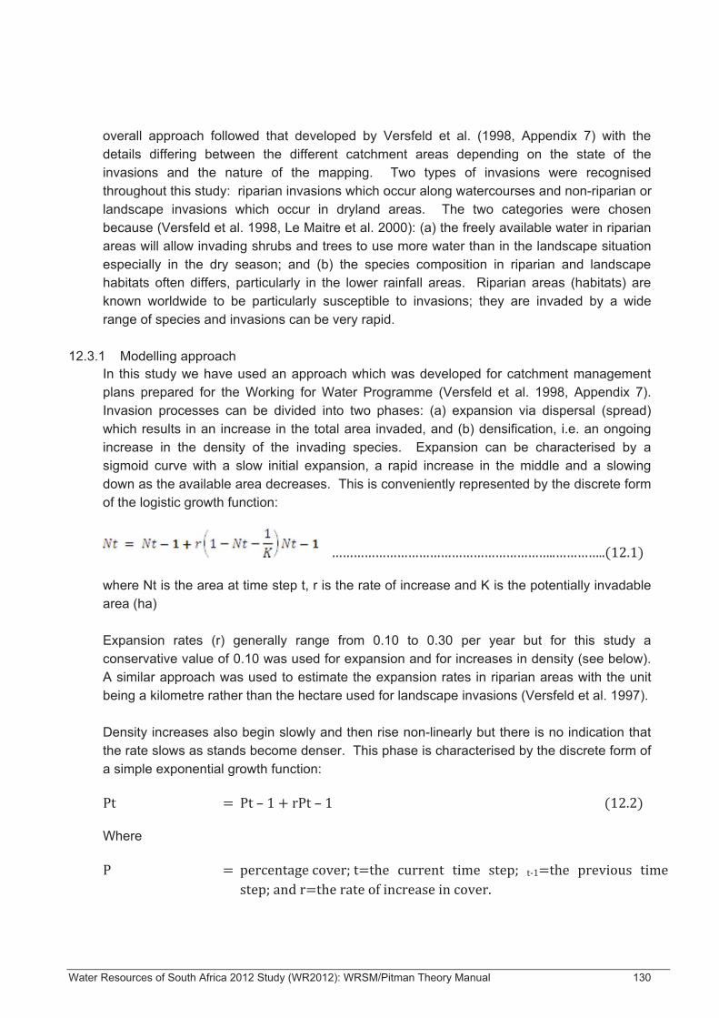
Water Resources of South Africa 2012 Study (WR2012): WRSM/Pitman Theory Manual 130
overall approach followed that developed by Versfeld et al. (1998, Appendix 7) with the details differing between the different catchment areas depending on the state of the invasions and the nature of the mapping. Two types of invasions were recognised throughout this study: riparian invasions which occur along watercourses and non-riparian or landscape invasions which occur in dryland areas. The two categories were chosen because (Versfeld et al. 1998, Le Maitre et al. 2000): (a) the freely available water in riparian areas will allow invading shrubs and trees to use more water than in the landscape situation especially in the dry season; and (b) the species composition in riparian and landscape habitats often differs, particularly in the lower rainfall areas. Riparian areas (habitats) are known worldwide to be particularly susceptible to invasions; they are invaded by a wide range of species and invasions can be very rapid.
12.3.1 Modelling approach In this study we have used an approach which was developed for catchment management plans prepared for the Working for Water Programme (Versfeld et al. 1998, Appendix 7). Invasion processes can be divided into two phases: (a) expansion via dispersal (spread) which results in an increase in the total area invaded, and (b) densification, i.e. an ongoing increase in the density of the invading species. Expansion can be characterised by a sigmoid curve with a slow initial expansion, a rapid increase in the middle and a slowing down as the available area decreases. This is conveniently represented by the discrete form of the logistic growth function:
where Nt is the area at time step t, r is the rate of increase and K is the potentially invadable area (ha) Expansion rates (r) generally range from 0.10 to 0.30 per year but for this study a conservative value of 0.10 was used for expansion and for increases in density (see below). A similar approach was used to estimate the expansion rates in riparian areas with the unit being a kilometre rather than the hectare used for landscape invasions (Versfeld et al. 1997). Density increases also begin slowly and then rise non-linearly but there is no indication that the rate slows as stands become denser. This phase is characterised by the discrete form of a simple exponential growth function:
Where
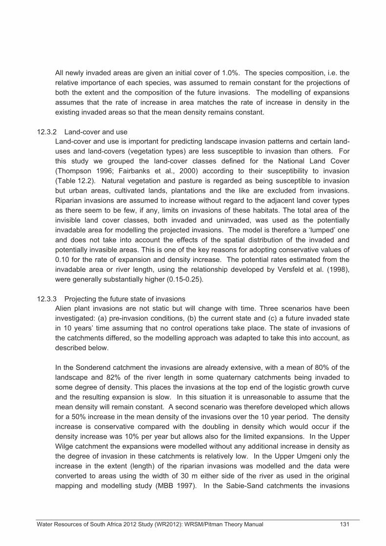
Water Resources of South Africa 2012 Study (WR2012): WRSM/Pitman Theory Manual 131
All newly invaded areas are given an initial cover of 1.0%. The species composition, i.e. the relative importance of each species, was assumed to remain constant for the projections of both the extent and the composition of the future invasions. The modelling of expansions assumes that the rate of increase in area matches the rate of increase in density in the existing invaded areas so that the mean density remains constant.
12.3.2 Land-cover and use Land-cover and use is important for predicting landscape invasion patterns and certain land-uses and land-covers (vegetation types) are less susceptible to invasion than others. For this study we grouped the land-cover classes defined for the National Land Cover (Thompson 1996; Fairbanks et al., 2000) according to their susceptibility to invasion (Table 12.2). Natural vegetation and pasture is regarded as being susceptible to invasion but urban areas, cultivated lands, plantations and the like are excluded from invasions. Riparian invasions are assumed to increase without regard to the adjacent land cover types as there seem to be few, if any, limits on invasions of these habitats. The total area of the invisible land cover classes, both invaded and uninvaded, was used as the potentially invadable area for modelling the projected invasions. The model is therefore a ‘lumped’ one and does not take into account the effects of the spatial distribution of the invaded and potentially invasible areas. This is one of the key reasons for adopting conservative values of 0.10 for the rate of expansion and density increase. The potential rates estimated from the invadable area or river length, using the relationship developed by Versfeld et al. (1998), were generally substantially higher (0.15-0.25).
12.3.3 Projecting the future state of invasions Alien plant invasions are not static but will change with time. Three scenarios have been investigated: (a) pre-invasion conditions, (b) the current state and (c) a future invaded state in 10 years’ time assuming that no control operations take place. The state of invasions of the catchments differed, so the modelling approach was adapted to take this into account, as described below. In the Sonderend catchment the invasions are already extensive, with a mean of 80% of the landscape and 82% of the river length in some quaternary catchments being invaded to some degree of density. This places the invasions at the top end of the logistic growth curve and the resulting expansion is slow. In this situation it is unreasonable to assume that the mean density will remain constant. A second scenario was therefore developed which allows for a 50% increase in the mean density of the invasions over the 10 year period. The density increase is conservative compared with the doubling in density which would occur if the density increase was 10% per year but allows also for the limited expansions. In the Upper Wilge catchment the expansions were modelled without any additional increase in density as the degree of invasion in these catchments is relatively low. In the Upper Umgeni only the increase in the extent (length) of the riparian invasions was modelled and the data were converted to areas using the width of 30 m either side of the river as used in the original mapping and modelling study (MBB 1997). In the Sabie-Sand catchments the invasions
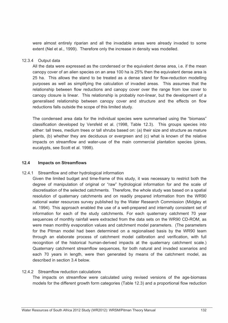
Water Resources of South Africa 2012 Study (WR2012): WRSM/Pitman Theory Manual 132
were almost entirely riparian and all the invadable areas were already invaded to some extent (Nel et al., 1999). Therefore only the increase in density was modelled.
12.3.4 Output data All the data were expressed as the condensed or the equivalent dense area, i.e. if the mean canopy cover of an alien species on an area 100 ha is 25% then the equivalent dense area is 25 ha. This allows the stand to be treated as a dense stand for flow-reduction modelling purposes as well as simplifying the calculation of invaded areas. This assumes that the relationship between flow reductions and canopy cover over the range from low cover to canopy closure is linear. This relationship is probably non-linear, but the development of a generalised relationship between canopy cover and structure and the effects on flow reductions falls outside the scope of this limited study. The condensed area data for the individual species were summarised using the “biomass” classification developed by Versfeld et al. (1998, Table 12.3). This groups species into either: tall trees, medium trees or tall shrubs based on: (a) their size and structure as mature plants, (b) whether they are deciduous or evergreen and (c) what is known of the relative impacts on streamflow and water-use of the main commercial plantation species (pines, eucalypts, see Scott et al. 1998).
12.4 Impacts on Streamflows
12.4.1 Streamflow and other hydrological information Given the limited budget and time-frame of this study, it was necessary to restrict both the degree of manipulation of original or “raw” hydrological information for and the scale of discretisation of the selected catchments. Therefore, the whole study was based on a spatial resolution of quaternary catchments and on readily prepared information from the WR90 national water resources survey published by the Water Research Commission (Midgley et al. 1994). This approach enabled the use of a well-prepared and internally consistent set of information for each of the study catchments. For each quaternary catchment 70 year sequences of monthly rainfall were extracted from the data sets on the WR90 CD-ROM, as were mean monthly evaporation values and catchment model parameters. (The parameters for the Pitman model had been determined on a regionalised basis by the WR90 team through an elaborate process of catchment model calibration and verification, with full recognition of the historical human-derived impacts at the quaternary catchment scale.) Quaternary catchment streamflow sequences, for both natural and invaded scenarios and each 70 years in length, were then generated by means of the catchment model, as described in section 3.4 below.
12.4.2 Streamflow reduction calculations The impacts on streamflow were calculated using revised versions of the age-biomass models for the different growth form categories (Table 12.3) and a proportional flow reduction
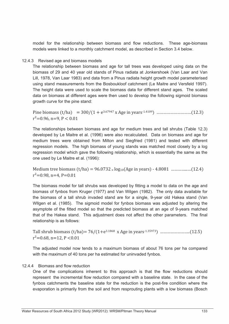
Water Resources of South Africa 2012 Study (WR2012): WRSM/Pitman Theory Manual 133
model for the relationship between biomass and flow reductions. These age-biomass models were linked to a monthly catchment model, as described in Section 3.4 below.
12.4.3 Revised age and biomass models The relationship between biomass and age for tall trees was developed using data on the biomass of 29 and 40 year old stands of Pinus radiata at Jonkershoek (Van Laar and Van Lill, 1978, Van Laar 1983) and data from a Pinus radiata height growth model parameterised using stand measurements from the Bosboukloof catchment (Le Maitre and Versfeld 1997). The height data were used to scale the biomass data for different stand ages. The scaled data on biomass at different ages were then used to develop the following sigmoid biomass growth curve for the pine stand:
The relationships between biomass and age for medium trees and tall shrubs (Table 12.3) developed by Le Maitre et al. (1996) were also recalculated. Data on biomass and age for medium trees were obtained from Milton and Siegfried (1981) and tested with different regression models. The high biomass of young stands was matched most closely by a log regression model which gave the following relationship, which is essentially the same as the one used by Le Maitre et al. (1996):
The biomass model for tall shrubs was developed by fitting a model to data on the age and biomass of fynbos from Kruger (1977) and Van Wilgen (1982). The only data available for the biomass of a tall shrub invaded stand are for a single, 9-year old Hakea stand (Van Wllgen et al. (1985). The sigmoid model for fynbos biomass was adjusted by altering the asymptote of the fitted model so that the predicted biomass at an age of 9-years matched that of the Hakea stand. This adjustment does not affect the other parameters. The final relationship is as follows:
The adjusted model now tends to a maximum biomass of about 76 tons per ha compared with the maximum of 40 tons per ha estimated for uninvaded fynbos.
12.4.4 Biomass and flow reduction One of the complications inherent to this approach is that the flow reductions should represent the incremental flow reduction compared with a baseline state. In the case of the fynbos catchments the baseline state for the reduction is the post-fire condition where the evaporation is primarily from the soil and from resprouting plants with a low biomass (Bosch
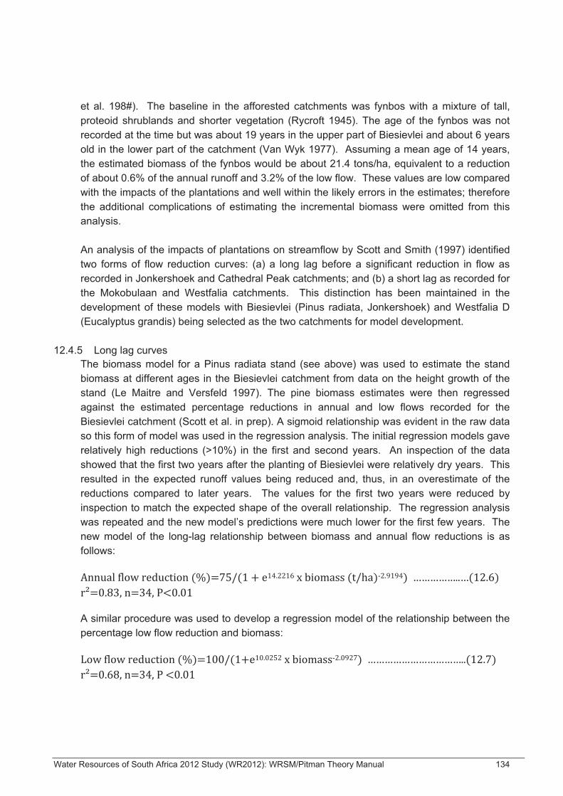
Water Resources of South Africa 2012 Study (WR2012): WRSM/Pitman Theory Manual 134
et al. 198#). The baseline in the afforested catchments was fynbos with a mixture of tall, proteoid shrublands and shorter vegetation (Rycroft 1945). The age of the fynbos was not recorded at the time but was about 19 years in the upper part of Biesievlei and about 6 years old in the lower part of the catchment (Van Wyk 1977). Assuming a mean age of 14 years, the estimated biomass of the fynbos would be about 21.4 tons/ha, equivalent to a reduction of about 0.6% of the annual runoff and 3.2% of the low flow. These values are low compared with the impacts of the plantations and well within the likely errors in the estimates; therefore the additional complications of estimating the incremental biomass were omitted from this analysis. An analysis of the impacts of plantations on streamflow by Scott and Smith (1997) identified two forms of flow reduction curves: (a) a long lag before a significant reduction in flow as recorded in Jonkershoek and Cathedral Peak catchments; and (b) a short lag as recorded for the Mokobulaan and Westfalia catchments. This distinction has been maintained in the development of these models with Biesievlei (Pinus radiata, Jonkershoek) and Westfalia D (Eucalyptus grandis) being selected as the two catchments for model development.
12.4.5 Long lag curves The biomass model for a Pinus radiata stand (see above) was used to estimate the stand biomass at different ages in the Biesievlei catchment from data on the height growth of the stand (Le Maitre and Versfeld 1997). The pine biomass estimates were then regressed against the estimated percentage reductions in annual and low flows recorded for the Biesievlei catchment (Scott et al. in prep). A sigmoid relationship was evident in the raw data so this form of model was used in the regression analysis. The initial regression models gave relatively high reductions (>10%) in the first and second years. An inspection of the data showed that the first two years after the planting of Biesievlei were relatively dry years. This resulted in the expected runoff values being reduced and, thus, in an overestimate of the reductions compared to later years. The values for the first two years were reduced by inspection to match the expected shape of the overall relationship. The regression analysis was repeated and the new model’s predictions were much lower for the first few years. The new model of the long-lag relationship between biomass and annual flow reductions is as follows:
A similar procedure was used to develop a regression model of the relationship between the percentage low flow reduction and biomass:
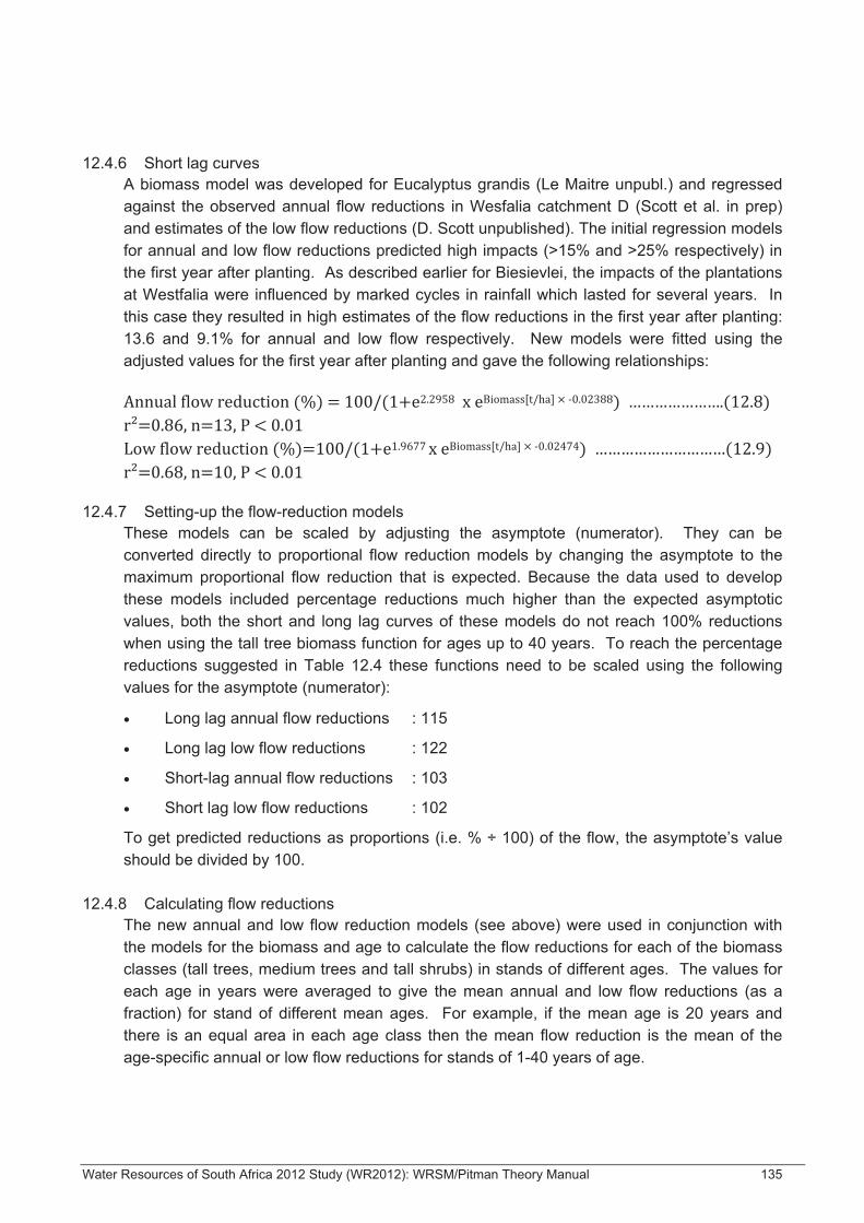
Water Resources of South Africa 2012 Study (WR2012): WRSM/Pitman Theory Manual 135
12.4.6 Short lag curves A biomass model was developed for Eucalyptus grandis (Le Maitre unpubl.) and regressed against the observed annual flow reductions in Wesfalia catchment D (Scott et al. in prep) and estimates of the low flow reductions (D. Scott unpublished). The initial regression models for annual and low flow reductions predicted high impacts (>15% and >25% respectively) in the first year after planting. As described earlier for Biesievlei, the impacts of the plantations at Westfalia were influenced by marked cycles in rainfall which lasted for several years. In this case they resulted in high estimates of the flow reductions in the first year after planting: 13.6 and 9.1% for annual and low flow respectively. New models were fitted using the adjusted values for the first year after planting and gave the following relationships:
12.4.7 Setting-up the flow-reduction models These models can be scaled by adjusting the asymptote (numerator). They can be converted directly to proportional flow reduction models by changing the asymptote to the maximum proportional flow reduction that is expected. Because the data used to develop these models included percentage reductions much higher than the expected asymptotic values, both the short and long lag curves of these models do not reach 100% reductions when using the tall tree biomass function for ages up to 40 years. To reach the percentage reductions suggested in Table 12.4 these functions need to be scaled using the following values for the asymptote (numerator):
• Long lag annual flow reductions : 115
• Long lag low flow reductions : 122
• Short-lag annual flow reductions : 103
• Short lag low flow reductions : 102
To get predicted reductions as proportions (i.e. % ÷ 100) of the flow, the asymptote’s value should be divided by 100.
12.4.8 Calculating flow reductions The new annual and low flow reduction models (see above) were used in conjunction with the models for the biomass and age to calculate the flow reductions for each of the biomass classes (tall trees, medium trees and tall shrubs) in stands of different ages. The values for each age in years were averaged to give the mean annual and low flow reductions (as a fraction) for stand of different mean ages. For example, if the mean age is 20 years and there is an equal area in each age class then the mean flow reduction is the mean of the age-specific annual or low flow reductions for stands of 1-40 years of age.
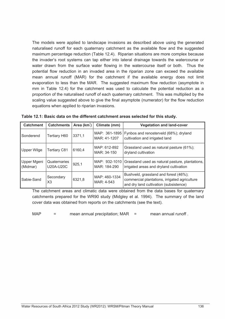
Water Resources of South Africa 2012 Study (WR2012): WRSM/Pitman Theory Manual 136
The models were applied to landscape invasions as described above using the generated naturalised runoff for each quaternary catchment as the available flow and the suggested maximum percentage reduction (Table 12.4). Riparian situations are more complex because the invader’s root systems can tap either into lateral drainage towards the watercourse or water drawn from the surface water flowing in the watercourse itself or both. Thus the potential flow reduction in an invaded area in the riparian zone can exceed the available mean annual runoff (MAR) for the catchment if the available energy does not limit evaporation to less than the MAR. The suggested maximum flow reduction (asymptote in mm in Table 12.4) for the catchment was used to calculate the potential reduction as a proportion of the naturalised runoff of each quaternary catchment. This was multiplied by the scaling value suggested above to give the final asymptote (numerator) for the flow reduction equations when applied to riparian invasions.
Table 12.1: Basic data on the different catchment areas selected for this study.
Catchment Catchments Area (km²) Climate (mm) Vegetation and land-cover
Sonderend Tertiary H60 3371,1 MAP: 361-1895MAR: 41-1207
Fynbos and renosterveld (68%); dryland cultivation and irrigated land
Upper Wilge Tertiary C81 6160,4 MAP: 612-892 MAR: 34-150
Grassland used as natural pasture (61%); dryland cultivation
Upper Mgeni (Midmar)
Quaternaries U20A-U20C 925,1 MAP: 932-1010
MAR: 184-290 Grassland used as natural pasture, plantations, irrigated areas and dryland cultivation
Sabie-Sand Secondary X3 6321,8 MAP: 460-1334
MAR: 4-543
Bushveld, grassland and forest (46%); commercial plantations, irrigated agriculture and dry land cultivation (subsistence)
The catchment areas and climatic data were obtained from the data bases for quaternary catchments prepared for the WR90 study (Midgley et al. 1994). The summary of the land cover data was obtained from reports on the catchments (see the text). MAP = mean annual precipitation; MAR = mean annual runoff .

Water Resources of South Africa 2012 Study (WR2012): WRSM/Pitman Theory Manual 137
Table 12.2: A summary of the invasibility of the different land-cover classes used for the National Land Cover Survey (Thompson 1996)
Invasibility for landscape invasions Land Cover Class
Not invasible All classes of Urban / built-up land Mines and Quarries All classes of Cultivated land Forest plantations Water bodies Barren Rock
Invasible All classes of natural vegetation Dongas & sheet erosion scars Wetlands All classes of Degraded land Improved and Unimproved Grassland
Wetlands are assumed to be invasible as most wetlands are seasonal dry, or have extensive seasonally dry areas which are subject to invasions in contrast to the permanently wet areas mapped as waterbodies. The areas involved are generally also small and unlikely to significantly influence the results.
Table 12.3: Alien species and associated biomass equations used in calculating the impact of invaders on water resources (after Versfeld et al. 1998)
Invading Alien Species Biomass Equation No. Invading Alien Species Biomass Equation No.
Acacia baileyana 2 Leptospermum laevigatum 1
Acacia cyclops 2 Melia azedarach # 2
Acacia decurrens 2 Morus alba # 2
Acacia elata 3 Nerium oleander 2
Acacia longifolia 2 Opuntia spp 1
Acacia mearnsii 3 Paraserianthes lophantha 1
Acacia melanoxylon 3 Pinus spp 3
Acacia pycnantha 2 Pittosporum undulatum 1
Acacia saligna 2 Populus spp # 3
Acacia spp 3 Prosopis spp 2
Alnus viridis 3 Psidium guajava 1
Arundo donax 2 Pyracantha sp 1
Caesalpinia decapetala 1 Quercus robur # 2
Chromolaena odorata 1 Robinia pseudoacacia # 2
Cupressus glabra 2 Rubus Sp 1
Eucalyptus spp 3 Salix spp # 2

Water Resources of South Africa 2012 Study (WR2012): WRSM/Pitman Theory Manual 138
Invading Alien Species Biomass Equation No. Invading Alien Species Biomass Equation No.
Ficus spp 3 Sesbania punicea 2
Gleditsia triacanthos # 2 Solanum mauritianum 1
Hakea spp 1 Tamarix spp 2
Jacaranda mimosifolia # 2 Uncertain 3
Lantana camara 1 Uncertain 3
Deciduous species are indicated with a #. For more information see the text.
Table 12.4: Values for parameters of the flow reduction equations for the different catchments, landscape and riparian invasions and annual and low flows
Catchment Situation Flow period Suggested Asymptote Mean age
(years) (%) (mm)
Sonderend landscape annual 83 7.5
low flow 85 7.5
riparian annual 100 500 20
low flow 100 30 20
Upper Wilge landscape annual 100 20
low flow 100 20
riparian annual 100 300 20
low flow 100 6 20
Upper Mngeni landscape annual 90 20
low flow 95 20
riparian annual 100 400 20
low flow 100 20 20
Sabie-Sand landscape annual 90 20
low flow 95 20
riparian annual 100 500 20
low flow 100 35 20
*Note: The low flow values represent the expected cumulative reduction over three low flow months that occur in the average year. The values for the suggested maximum percentage and absolute reductions were selected to match the growing conditions in the different catchments. The mean age of the invaders in the different situations was based on the estimates of Versfeld et al. (1998).
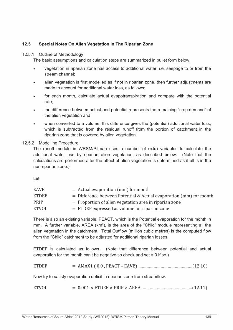
Water Resources of South Africa 2012 Study (WR2012): WRSM/Pitman Theory Manual 139
12.5 Special Notes On Alien Vegetation In The Riparian Zone
12.5.1 Outline of Methodology The basic assumptions and calculation steps are summarized in bullet form below.
• vegetation in riparian zone has access to additional water, i.e. seepage to or from the stream channel;
• alien vegetation is first modelled as if not in riparian zone, then further adjustments are made to account for additional water loss, as follows;
• for each month, calculate actual evapotranspiration and compare with the potential rate;
• the difference between actual and potential represents the remaining “crop demand” of the alien vegetation and
• when converted to a volume, this difference gives the (potential) additional water loss, which is subtracted from the residual runoff from the portion of catchment in the riparian zone that is covered by alien vegetation.
12.5.2 Modelling Procedure The runoff module in WRSM/Pitman uses a number of extra variables to calculate the additional water use by riparian alien vegetation, as described below. (Note that the calculations are performed after the effect of alien vegetation is determined as if all is in the non-riparian zone.) Let
There is also an existing variable, PEACT, which is the Potential evaporation for the month in mm. A further variable, AREA (km²), is the area of the “Child” module representing all the alien vegetation in the catchment. Total Outflow (million cubic metres) is the computed flow from the “Child” catchment to be adjusted for additional riparian losses. ETDEF is calculated as follows. (Note that difference between potential and actual evaporation for the month can’t be negative so check and set = 0 if so.)
Now try to satisfy evaporation deficit in riparian zone from streamflow.

Water Resources of South Africa 2012 Study (WR2012): WRSM/Pitman Theory Manual 140
The final step is to subtract ETVOL from TotalOutflow (or set it to zero if ETVOL is greater than TotalOutflow) as follows:
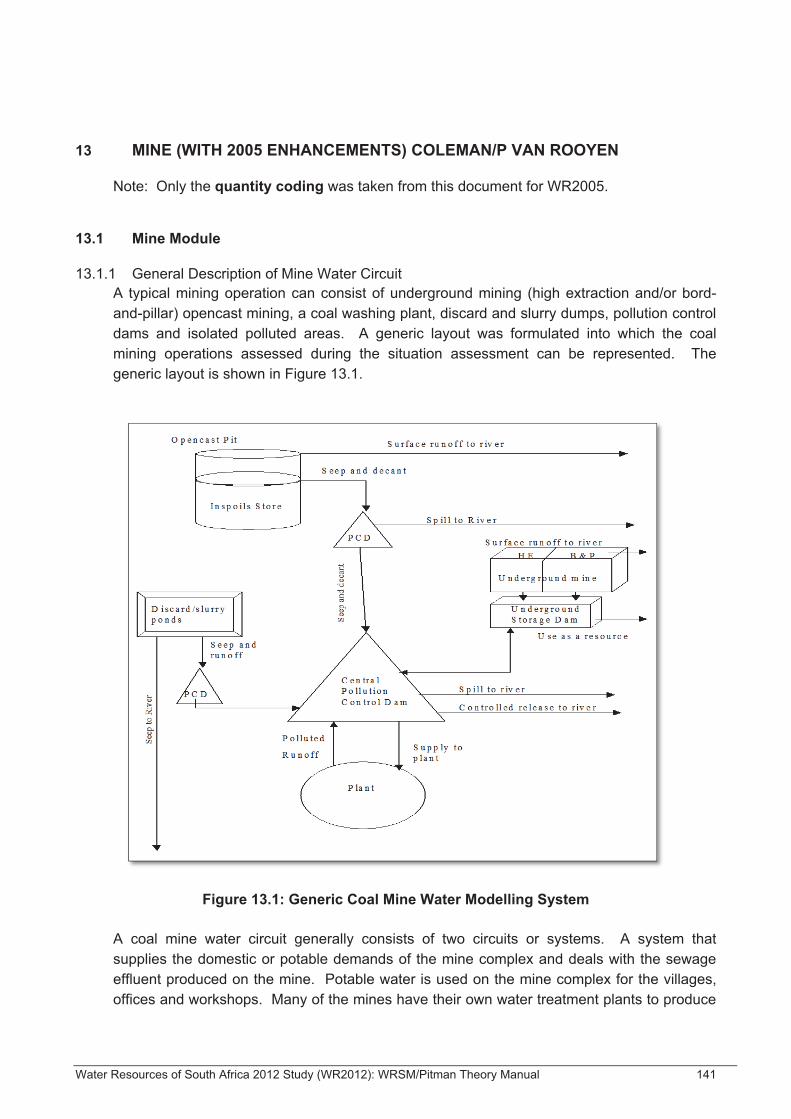
Water Resources of South Africa 2012 Study (WR2012): WRSM/Pitman Theory Manual 141
13 MINE (WITH 2005 ENHANCEMENTS) COLEMAN/P VAN ROOYEN
Note: Only the quantity coding was taken from this document for WR2005.
13.1 Mine Module
13.1.1 General Description of Mine Water Circuit A typical mining operation can consist of underground mining (high extraction and/or bord-and-pillar) opencast mining, a coal washing plant, discard and slurry dumps, pollution control dams and isolated polluted areas. A generic layout was formulated into which the coal mining operations assessed during the situation assessment can be represented. The generic layout is shown in Figure 13.1.
Figure 13.1: Generic Coal Mine Water Modelling System A coal mine water circuit generally consists of two circuits or systems. A system that supplies the domestic or potable demands of the mine complex and deals with the sewage effluent produced on the mine. Potable water is used on the mine complex for the villages, offices and workshops. Many of the mines have their own water treatment plants to produce

Water Resources of South Africa 2012 Study (WR2012): WRSM/Pitman Theory Manual 142
the required potable water. The raw water for this circuit can be abstracted from a borehole, a river or dam, supplied from Eskom, or supplied by a municipality. The mines generally have sewage treatment plants (STP) on the complex to deal with the sewerage. The effluent from the STP can be used for irrigation, dust suppression, or released to the river system as a point source. This circuit is treated in the water quality model as an abstraction and a point source return flow via the STP. The other circuit on a mine complex is the polluted water circuit. The water in the dirty water circuit could include runoff from dirty catchment areas collected in pollution control dams, the return water from a slurry disposal facility, decant or water make from an opencast pit and water pumped from underground. A sub-module has been developed for an opencast pit, an underground mining section, a dirty catchment area and dumps. These outputs from these modules are connected as per Figure 13.1 to represent a particular coal mine. The generic layout of the polluted water circuit is shown in Figure 13.1. Figure 13.1 shows, for illustrative purposes only, a single opencast pit and underground mining section. However provision has been made in the model for up to 10 pits, 10 underground section and 10 dumps for a particular mine complex. The coal beneficiation plant is the main water demand centre on a coal complex. The plant is often supplied with recycled polluted water from the mines polluted water circuit with make-up water perhaps being supplied from the potable water circuit. The quantity of water used at the plant is a function of the coal throughput and the type of beneficiation process employed at the plant. A time series of water demands are input to the model over the simulation period. These demands being met with water from the central pollution control dam. Practically on a mine complex, there are a number of pollution control dams (PCD). In the generic representation of the complex these have been lumped into a single pollution control dam called the central pollution control dam. This PCD receives water from the underground mine section, the opencast section, the discard dump/slurry pond (PCD) and polluted runoff from the dirty areas on the complex. Allowance has been made for the water stored in the central PCD to be pumped underground. This management option is practiced on some mines.
13.2 Opencast Sub-module
13.2.1 Introduction An opencast mining operation is complex in terms of the mining plan, water pathways and water quality. Detailed models are available for modelling the water quality and water make of an opencast pit. However, given that the WRPM is a planning model, the detailed description of the mining process used in these models is not necessary to describe the

Water Resources of South Africa 2012 Study (WR2012): WRSM/Pitman Theory Manual 143
general behaviour of a pit. The information collected on the opencast mining operations during the situation assessment included:-
• the reserve area for the different pits on a particular mine complex;
• the start and end date of the mining operation on each of the pits;
• the current area mined;
• details of the current and future rehabilitation;
• the decant level and final storage volume after closure and
• when available, the closure plans for the pits.
The opencast component of the mine module was formulated so that the opencast pit model can accommodate the different configurations found on the various mines in the catchment. An opencast mine can essentially be in three states viz.:-
• pre-mining that is in an undisturbed or natural state;
• operational pit and
• post mining, i.e. a closed pit.
The model has been formulated so that all three states can be included in a single model framework.
13.2.2 Structure of model During the life of mine of a pit, the opencast mine could consist of the following components (See Figure 13.2):-
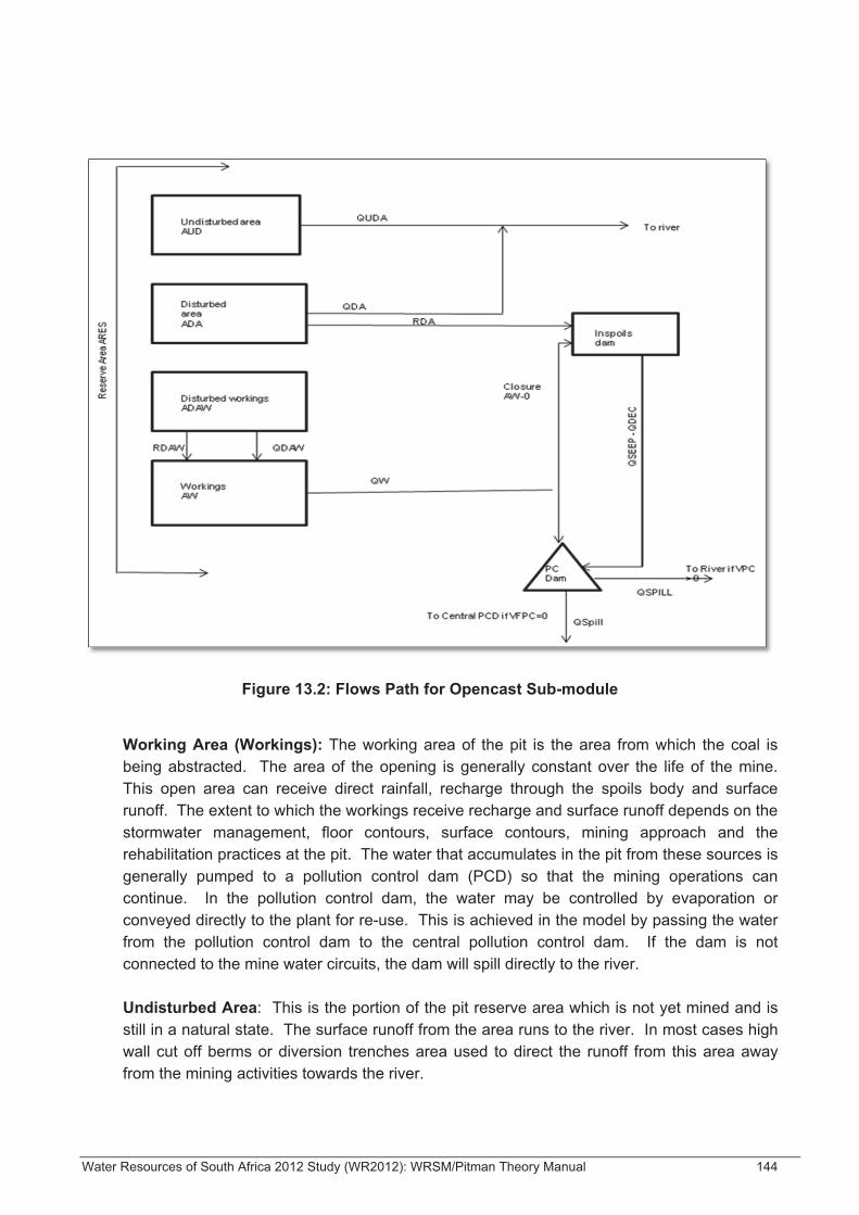
Water Resources of South Africa 2012 Study (WR2012): WRSM/Pitman Theory Manual 144
Figure 13.2: Flows Path for Opencast Sub-module
Working Area (Workings): The working area of the pit is the area from which the coal is being abstracted. The area of the opening is generally constant over the life of the mine. This open area can receive direct rainfall, recharge through the spoils body and surface runoff. The extent to which the workings receive recharge and surface runoff depends on the stormwater management, floor contours, surface contours, mining approach and the rehabilitation practices at the pit. The water that accumulates in the pit from these sources is generally pumped to a pollution control dam (PCD) so that the mining operations can continue. In the pollution control dam, the water may be controlled by evaporation or conveyed directly to the plant for re-use. This is achieved in the model by passing the water from the pollution control dam to the central pollution control dam. If the dam is not connected to the mine water circuits, the dam will spill directly to the river. Undisturbed Area: This is the portion of the pit reserve area which is not yet mined and is still in a natural state. The surface runoff from the area runs to the river. In most cases high wall cut off berms or diversion trenches area used to direct the runoff from this area away from the mining activities towards the river.
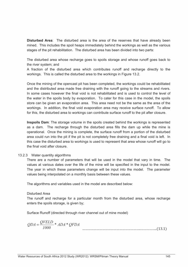
Water Resources of South Africa 2012 Study (WR2012): WRSM/Pitman Theory Manual 145
Disturbed Area: The disturbed area is the area of the reserves that have already been mined. This includes the spoil heaps immediately behind the workings as well as the various stages of the pit rehabilitation. The disturbed area has been divided into two parts: The disturbed area whose recharge goes to spoils storage and whose runoff goes back to the river system; and A fraction of the disturbed area which contributes runoff and recharge directly to the workings. This is called the disturbed area to the workings in Figure 13.2. Once the mining of the opencast pit has been completed, the workings could be rehabilitated and the distributed area made free draining with the runoff going to the streams and rivers. In some cases however the final void is not rehabilitated and is used to control the level of the water in the spoils body by evaporation. To cater for this case in the model, the spoils store can be given an evaporation area. This area need not be the same as the area of the workings. In addition, the final void evaporation area may receive surface runoff. To allow for this, the disturbed area to workings can contribute surface runoff to the pit after closure. Inspoils Dam: The storage volume in the spoils created behind the workings is represented as a dam. The recharge through the disturbed area fills the dam up while the mine is operational. Once the mining is complete, the surface runoff from a portion of the disturbed area could run into the pit if the pit is not completely free draining and a final void is left. In this case the disturbed area to workings is used to represent that area whose runoff will go to the final void after closure.
13.2.3 Water quantity algorithms
There are a number of parameters that will be used in the model that vary in time. The values at various dates over the life of the mine will be specified in the input to the model. The year in which these parameters change will be input into the model. The parameter values being interpolated on a monthly basis between these values. The algorithms and variables used in the model are described below: Disturbed Area The runoff and recharge for a particular month from the disturbed area, whose recharge enters the spoils storage, is given by; Surface Runoff (directed through river channel out of mine model)
QFDA* ADA* 1000
QVELD QDA =

Water Resources of South Africa 2012 Study (WR2012): WRSM/Pitman Theory Manual 146
Recharge
RFDA* ADA* 1000
RAOM RDA =
Where:
• QDA is the runoff volume from the disturbed area in million m³ /month;
• QVELD(mm) is the unit runoff from the naturalized catchment surface (from desegregation of QP);
• ADA (km²) is the disturbed area for the particular month being computed. This is time varying input parameter. The value for the computation month is interpolated from annual input values;
• QFDA is a runoff factor to adjust the natural runoff for the change in surface conditions of the disturbed area (constant over simulation period);
• RDA is the recharge volume through the disturbed area in million m³/month;
• RAIN (mm) is the rainfall for the month and
• RFDA is the fraction of the rainfall that will infiltrate below the upper soil layers to recharge the spoils storage. This factor will vary from month to month depending on the season. A value is input for each month. These values remaining constant over the simulation period.
13.2.3.1 Disturbed area to workings
The runoff and recharge that will enter the workings during the operation of the opencast pit is given by: Surface Runoff
QFDAW* ADAW* 1000
QVELD QDAW =
Where
• QDAW is the runoff from the disturbed area in million m³ / month;
• ADAW is the area (km²) of the disturbed area whose runoff and recharge enters the workings during the pit operation. After closure the runoff from the area will enter the final void if it is not rehabilitated. ADAW is a time varying input parameter whose values are interpolated from annual input values;
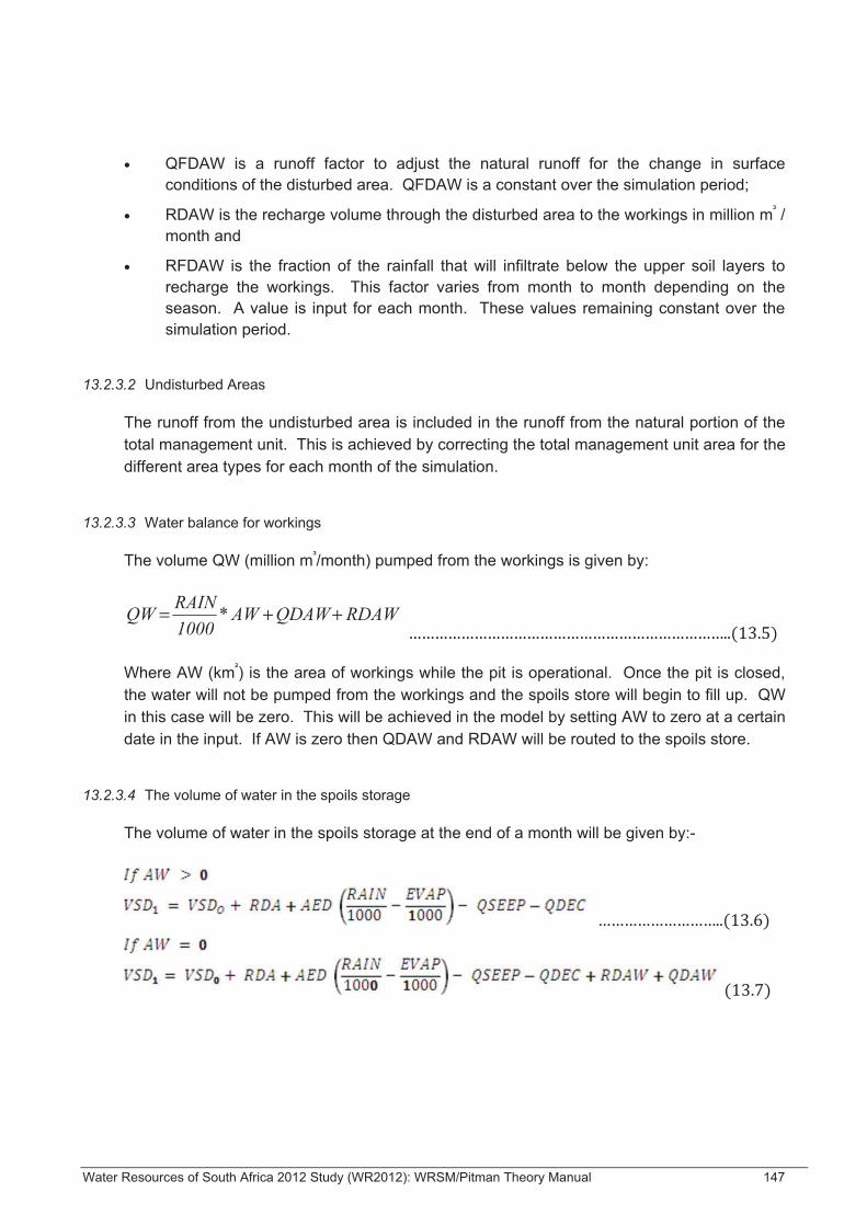
Water Resources of South Africa 2012 Study (WR2012): WRSM/Pitman Theory Manual 147
• QFDAW is a runoff factor to adjust the natural runoff for the change in surface conditions of the disturbed area. QFDAW is a constant over the simulation period;
• RDAW is the recharge volume through the disturbed area to the workings in million m³ / month and
• RFDAW is the fraction of the rainfall that will infiltrate below the upper soil layers to recharge the workings. This factor varies from month to month depending on the season. A value is input for each month. These values remaining constant over the simulation period.
13.2.3.2 Undisturbed Areas
The runoff from the undisturbed area is included in the runoff from the natural portion of the total management unit. This is achieved by correcting the total management unit area for the different area types for each month of the simulation.
13.2.3.3 Water balance for workings
The volume QW (million m³/month) pumped from the workings is given by:
RDAWQDAWAW1000RAIN QW ++= *
Where AW (km²) is the area of workings while the pit is operational. Once the pit is closed, the water will not be pumped from the workings and the spoils store will begin to fill up. QW in this case will be zero. This will be achieved in the model by setting AW to zero at a certain date in the input. If AW is zero then QDAW and RDAW will be routed to the spoils store.
13.2.3.4 The volume of water in the spoils storage
The volume of water in the spoils storage at the end of a month will be given by:-

Water Resources of South Africa 2012 Study (WR2012): WRSM/Pitman Theory Manual 148
To determine the seeps, decants and volumes, the following procedure is followed:
Where
• VSD is the volume of water in the inspoils store in million m³. The subscripts 0 and 1 represent the start and end of month respectively;
• AED is the evaporation area (km²) that can be assigned to the inspoils store. This is used to simulate the closure plans employed by some lines to evaporate the pit water make from the opencast pit final voids. The parameters AED varies in time and values will be specified in the input;
• QSEEP (million m³/month) is the water that can seep from an opencast pit through the weathered zone in the soil profile;
• VSDS (million m³) is the storage volume in the spoils store at which seepage through the weathered zone can start. This is a time varying input parameter;
• VSDD (million m³) is the storage volume in the spoils store at which decant occurs. This is a time varying input parameter;
• Exp1 is an exponent;
• QSEEPMAX is the max seepage rate (million m³/month) that can occur from the spoils store when VSD0 VSDD. The value for this variable input to the program;
• QDEC is the volume of water that decants from the spoils store in million m³/month when VSD0 VSDD and
• EVAP is the monthly evaporation depth (mm/month).
13.2.3.5 Water Balance PCD
If
Water Resources of South Africa 2012 Study (WR2012): WRSM/Pitman Theory Manual 149
If
QSPILL goes to central pollution control dam If
QSPILL goes to the river Where
• VPC is the volume of water in the pollution control dam. The subscript 0 and 1 refers to the volume at the start and end of the month respectively;
• AFPC is the surface area of the pollution control dam (km²);
• VFPC is the full storage capacity of the pollution control dam (million m³) and
• QSPILL is the overflow from the pollution control dam (million m³/month).
13.3 Underground Sub-Module
13.3.1 Water Quantity Algorithms The underground sub-module consists of an underground storage dam, two undermined surface areas immediately above the storage dam and an upstream catchment whose runoff passes over the high extraction undermined area. One of the areas represents the area undermined by high extraction mining and the other the area undermined by bord and pillar mining. Both high extracting and bord and pillar mining techniques can therefore be accommodated in the modelling framework. The flow paths of the sub-module are shown in Figure 13.3. There is a recharge to the underground storage tank which is a function of the recharge through the catchment surface, groundwater and a fraction of the recharge through the catchment surface, groundwater and fraction of the runoff from the upstream catchment. During operation. water can be pumped from underground or excess water on the mine complex can be pumped underground. This pathway is represented as a constant flow to or from the central pollution control dam.

Water Resources of South Africa 2012 Study (WR2012): WRSM/Pitman Theory Manual 150
Figure 13.3: Flow Path for Underground Sub-module
The surface runoff from the upstream catchment is given by:
Where:
• QUP is the surface runoff volume from the upstream catchment in million m³/month;
• AUP is the area (km²) of the catchment upstream of the undermined catchment. This variable will be kept constant over the simulation period and
• QPER is the unit runoff from the associated salt washoff model (mm).
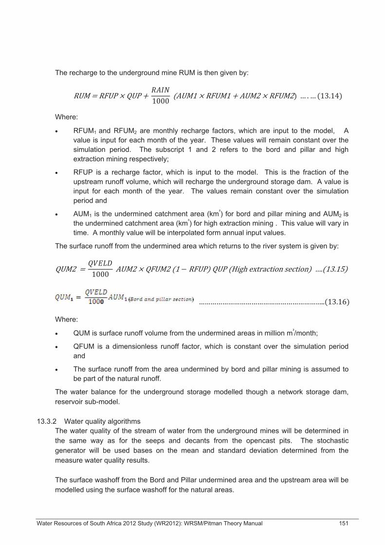
Water Resources of South Africa 2012 Study (WR2012): WRSM/Pitman Theory Manual 151
The recharge to the underground mine RUM is then given by:
Where:
• RFUM1 and RFUM2 are monthly recharge factors, which are input to the model, A value is input for each month of the year. These values will remain constant over the simulation period. The subscript 1 and 2 refers to the bord and pillar and high extraction mining respectively;
• RFUP is a recharge factor, which is input to the model. This is the fraction of the upstream runoff volume, which will recharge the underground storage dam. A value is input for each month of the year. The values remain constant over the simulation period and
• AUM1 is the undermined catchment area (km²) for bord and pillar mining and AUM2 is the undermined catchment area (km²) for high extraction mining . This value will vary in time. A monthly value will be interpolated form annual input values.
The surface runoff from the undermined area which returns to the river system is given by:
Where:
• QUM is surface runoff volume from the undermined areas in million m³/month;
• QFUM is a dimensionless runoff factor, which is constant over the simulation period and
• The surface runoff from the area undermined by bord and pillar mining is assumed to be part of the natural runoff.
The water balance for the underground storage modelled though a network storage dam, reservoir sub-model.
13.3.2 Water quality algorithms The water quality of the stream of water from the underground mines will be determined in the same way as for the seeps and decants from the opencast pits. The stochastic generator will be used bases on the mean and standard deviation determined from the measure water quality results. The surface washoff from the Bord and Pillar undermined area and the upstream area will be modelled using the surface washoff for the natural areas.

Water Resources of South Africa 2012 Study (WR2012): WRSM/Pitman Theory Manual 152
13.4 Discard/Slurry Ponds
13.4.1 Water quantity algorithms The slurry ponds and discard dumps generally have a decant system to drain the rainwater and the supernatant from the tops of the dumps to a return water dam. In addition to the decant, seepage and surface runoff from the dump is often collected in a system of drains and trenches and conveyed to the return water dam. In developing the dump model, the assumption has been made that a fraction of the slurry water leaving the plant is returned to the plant from the return water dam. Rather than model the complete slurry water circuit, the water demand at the plant is reduced to allow the recycle of slurry water. The modelling of the discard dump is then reduced to the prediction of spills from the return water dam due to the runoff from the dump surface, seepage from the dump and rainfall directly on the dam surface. The flow pathways are shown in Figure 13.4. These consist of a surface runoff and a seepage flow. The seepage flow can be split with a fraction going to the pollution control dam and a fraction directly to the river.

Water Resources of South Africa 2012 Study (WR2012): WRSM/Pitman Theory Manual 153
Figure 13.4: Flow Path for Discard Dump
The surface runoff volume QDMP (million m³/month) is given by:
Where: ADMP (km²) is the surface area of the dump. This is a time varying input parameter. The value for a month is interpolated from annual input values. QFDMP is a runoff factor for the dump. This factor is constant over the simulation period. The seep volume QSDMP (million m³/month) is given by:
Where:
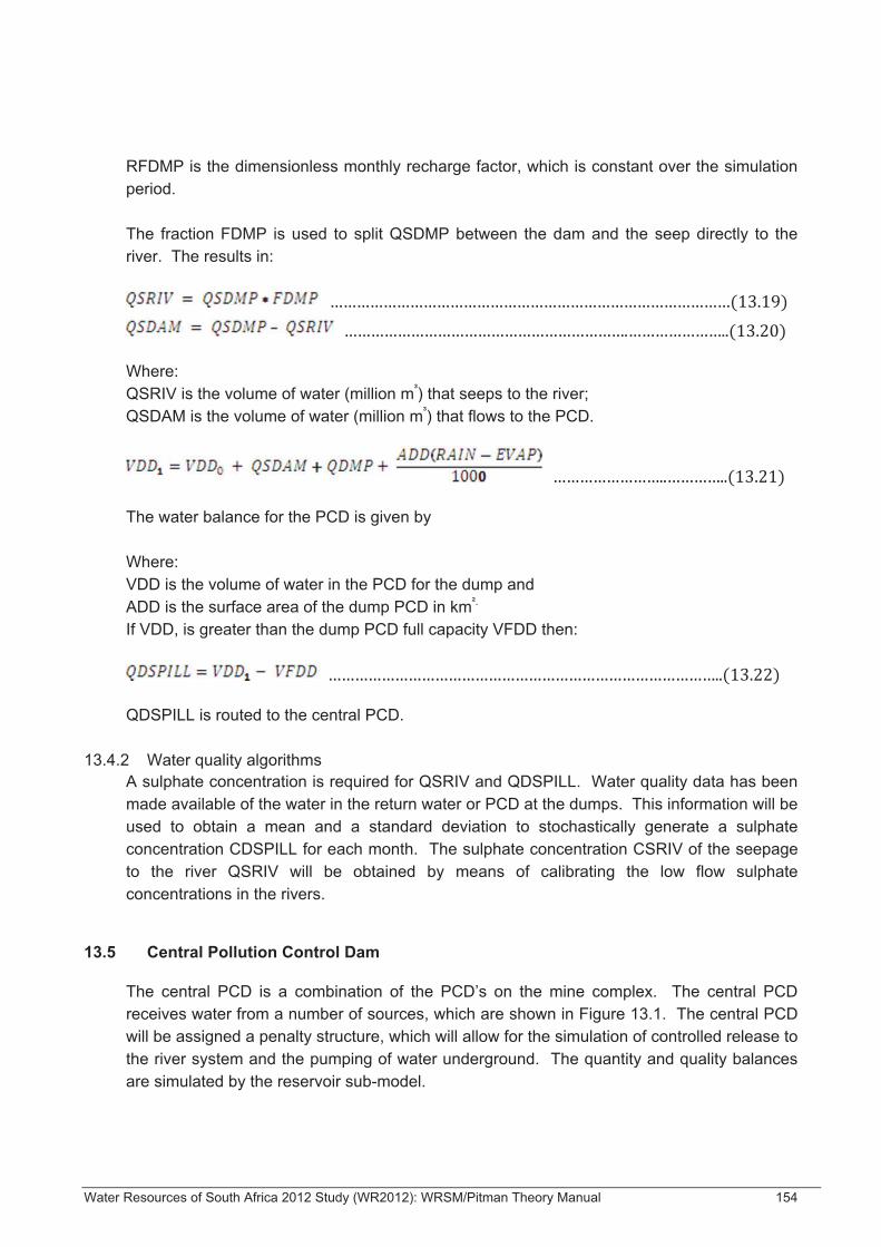
Water Resources of South Africa 2012 Study (WR2012): WRSM/Pitman Theory Manual 154
RFDMP is the dimensionless monthly recharge factor, which is constant over the simulation period. The fraction FDMP is used to split QSDMP between the dam and the seep directly to the river. The results in:
Where: QSRIV is the volume of water (million m³) that seeps to the river; QSDAM is the volume of water (million m³) that flows to the PCD.
The water balance for the PCD is given by Where: VDD is the volume of water in the PCD for the dump and ADD is the surface area of the dump PCD in km². If VDD, is greater than the dump PCD full capacity VFDD then:
QDSPILL is routed to the central PCD.
13.4.2 Water quality algorithms A sulphate concentration is required for QSRIV and QDSPILL. Water quality data has been made available of the water in the return water or PCD at the dumps. This information will be used to obtain a mean and a standard deviation to stochastically generate a sulphate concentration CDSPILL for each month. The sulphate concentration CSRIV of the seepage to the river QSRIV will be obtained by means of calibrating the low flow sulphate concentrations in the rivers.
13.5 Central Pollution Control Dam
The central PCD is a combination of the PCD’s on the mine complex. The central PCD receives water from a number of sources, which are shown in Figure 13.1. The central PCD will be assigned a penalty structure, which will allow for the simulation of controlled release to the river system and the pumping of water underground. The quantity and quality balances are simulated by the reservoir sub-model.
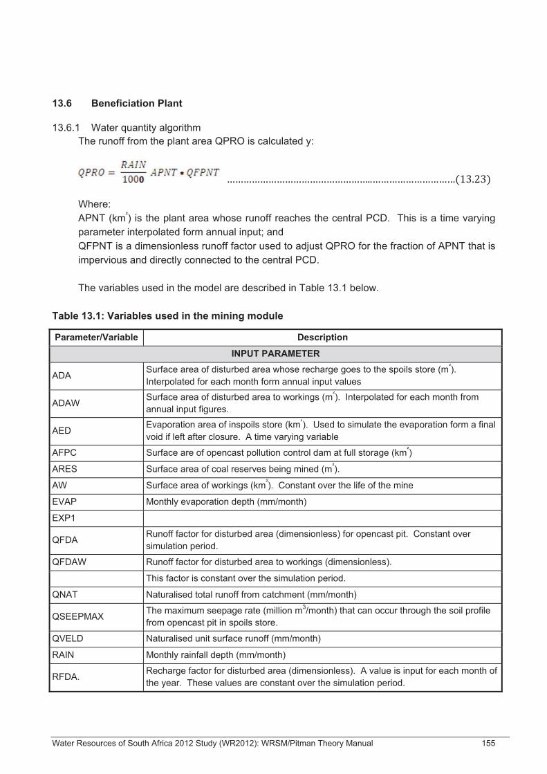
Water Resources of South Africa 2012 Study (WR2012): WRSM/Pitman Theory Manual 155
13.6 Beneficiation Plant
13.6.1 Water quantity algorithm The runoff from the plant area QPRO is calculated y:
Where: APNT (km²) is the plant area whose runoff reaches the central PCD. This is a time varying parameter interpolated form annual input; and QFPNT is a dimensionless runoff factor used to adjust QPRO for the fraction of APNT that is impervious and directly connected to the central PCD. The variables used in the model are described in Table 13.1 below.
Table 13.1: Variables used in the mining module
Parameter/Variable Description
INPUT PARAMETER
ADA Surface area of disturbed area whose recharge goes to the spoils store (m²). Interpolated for each month form annual input values
ADAW Surface area of disturbed area to workings (m²). Interpolated for each month from annual input figures.
AED Evaporation area of inspoils store (km²). Used to simulate the evaporation form a final void if left after closure. A time varying variable
AFPC Surface are of opencast pollution control dam at full storage (km²)
ARES Surface area of coal reserves being mined (m²).
AW Surface area of workings (km²). Constant over the life of the mine
EVAP Monthly evaporation depth (mm/month)
EXP1
QFDA Runoff factor for disturbed area (dimensionless) for opencast pit. Constant over simulation period.
QFDAW Runoff factor for disturbed area to workings (dimensionless).
This factor is constant over the simulation period.
QNAT Naturalised total runoff from catchment (mm/month)
QSEEPMAX The maximum seepage rate (million m3/month) that can occur through the soil profile from opencast pit in spoils store.
QVELD Naturalised unit surface runoff (mm/month)
RAIN Monthly rainfall depth (mm/month)
RFDA. Recharge factor for disturbed area (dimensionless). A value is input for each month of the year. These values are constant over the simulation period.
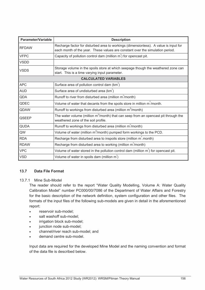
Water Resources of South Africa 2012 Study (WR2012): WRSM/Pitman Theory Manual 156
Parameter/Variable Description
RFDAW Recharge factor for disturbed area to workings (dimensionless). A value is input for each month of the year. These values are constant over the simulation period.
VFPC Capacity of pollution control dam (million m³) for opencast pit.
VSDD
VSDS Storage volume in the spoils store at which seepage though the weathered zone can start. This is a time varying input parameter.
CALCULATED VARIABLES
APC Surface area of pollution control dam (km²)
AUD Surface area of undisturbed area (km²)
QDA Runoff to river from disturbed area (million m³/month)
QDEC Volume of water that decants from the spoils store in million m³/month.
QDAW Runoff to workings from disturbed area (million m3/month)
QSEEP The water volume (million m3/month) that can seep from an opencast pit through the weathered zone of the soil profile.
QUDA Runoff to workings from disturbed area (million m³/month)
QW Volume of water (million m3/month) pumped form workings to the PCD.
RDA Recharge from disturbed area to inspoils store (million m³.month)
RDAW Recharge from disturbed area to working (million m³/month)
VPC Volume of water stored in the pollution control dam (million m³) for opencast pit.
VSD Volume of water in spoils dam (million m³)
13.7 Data File Format
13.7.1 Mine Sub-Model The reader should refer to the report “Water Quality Modelling, Volume A: Water Quality Calibration Model” number PC000/00/7086 of the Department of Water Affairs and Forestry for the basic description of the network definition, system configuration and other files. The formats of the input files of the following sub-models are given in detail in the aforementioned report: • reservoir sub-model; • salt washoff sub-model; • irrigation block sub-model; • junction node sub-model; • channel/river reach sub-model; and • demand centre sub-model.
Input data are required for the developed Mine Model and the naming convention and format of the data file is described below.

Water Resources of South Africa 2012 Study (WR2012): WRSM/Pitman Theory Manual 157
The file name for the Mine Sub-model uses the same naming convention as described in the above-mentioned report and a typical name for a mine sub-model file would be “mimm300.dat “. Where “mi” refers to the system identification code, “mm” indicates that the specific file contains data for a Mine Sub-model and “300” refers to a unique number assigned to the particular sub-model.
Water Resources of South Africa 2012 Study (WR2012): WRSM/Pitman Theory Manual 158
14 DAILY TIME STEP MODEL
14.1 Introduction
A Pitman daily time step model has been in existence since 1976 but remained in its original DOS form until a couple of years ago when it was decided to transform it into a similar model to the WRSM/Pitman monthly time step. A report entitled “A Mathematical Model for Generating Daily River Flows from Meteorological Data in South Africa” (Pitman W.V, 1976) was written by Dr Bill Pitman in March 1976 and contains a detailed methodology and all the tests carried out on a number of catchments. The WRSM/Pitman User Guide also explains how the user should prepare data, analyse a system and obtain results in the form of hydrographs and time series daily streamflow.
14.2 Methodology
The full methodology has not been repeated here but has rather been summarised with insight provided as to how it was incorporated into a model similar to the WRSM/Pitman monthly time step. A daily time step is often necessary to analyse streamflow from an ecological point of view and also in operating dams, designing river diversion works, coffer dams and off-channel dams. The WRSM/Pitman daily time step model was designed to generate daily flows using as input daily and monthly rainfall and average monthly potential evaporation. The structure is similar to that of the monthly time step with similar calibration parameters. Figure 14.1 shows a flowchart representation of the model. Assumed soil moisture conditions is determined from initial catchment discharge, precipitation is stored as interception and as soil moisture and this is subject to evaporation and transpiration. The quantity of precipitation that is not absorbed by the soil is the source of surface runoff. A portion of the precipitation held as soil moisture percolates into groundwater before entering the river system. The various components are suitably lagged and the total runoff at the catchment outlet is computed on a mass balance basis. The model has been designed to balance the catchment’s water budget and hence to determine the runoff using different time steps. For days during which there is no rain, a one-day time step is used. When a rain-day is encountered, the duration of the fall is estimated and the rainfall total is distributed as hourly amounts in order that the water budget may be computed at one-hour time intervals. After cessation of the storm a single time step of n hours is employed, where n = 24 – duration of the rainfall. It is thus evident that the onset of rain is assumed to coincide with the beginning of the day. Duration of rainfall is assumed via the following linear equation and is then rounded to the nearest whole number of hours.
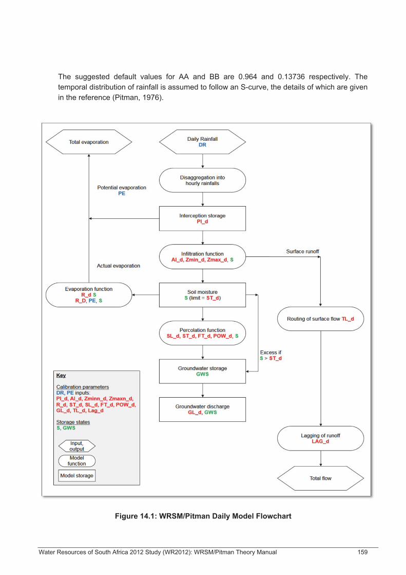
Water Resources of South Africa 2012 Study (WR2012): WRSM/Pitman Theory Manual 159
The suggested default values for AA and BB are 0.964 and 0.13736 respectively. The temporal distribution of rainfall is assumed to follow an S-curve, the details of which are given in the reference (Pitman, 1976).
Figure 14.1: WRSM/Pitman Daily Model Flowchart
Water Resources of South Africa 2012 Study (WR2012): WRSM/Pitman Theory Manual 160
Regarding interception, vegetation and soil surfaces may be initially dry before a fall of rain and a small amount of moisture is needed to wet these surfaces before runoff and infiltration can occur. This function is represented by assuming an interception storage (PI_d) which must be filled before precipitation is available for infiltration and runoff. Moisture from interception storage is removed at the potential evapotranspiration rate until all moisture is exhausted. Regarding surface runoff, it is taken to be derived from two sources namely: Runoff from impervious areas and Runoff resulting from rainfall that has not infiltrated into the soil. The first component is computed by multiplying the rainfall available for infiltration and runoff by the area of catchment that is impervious. The impervious area (AI_d) is the proportion of the catchment that contributes directly to surface runoff. Impervious areas not directly connected to water courses must flow over pervious areas before reaching a stream channel. Isolated impervious areas are therefore not included in parameter AI_d. For the second component, it was recognised that infiltration would be highly unlikely to be uniform throughout the catchment. The spatial distribution of infiltration rate is no doubt strongly influenced by physical features such as geology, soil type, vegetation and many others too numerous to mention. In most natural catchments these factors would result in a considerable spatial variation in infiltration rate. It was felt that a reasonable approximation could be reached by assuming a triangular frequency distribution of infiltration rate, thus reducing to a manageable number the parameters relating to this phenomenon. As in the case of the monthly model a symmetrical triangular frequency distribution was adopted using Zminn_d and Zmaxn_d. However, the daily model allows for the infiltration capacity to vary with the soil moisture status, unlike the monthly model. Further details and mathematical equations are available in the reference (Pitman, 1976). Regarding infiltration, the quantity of water entering storage as soil moisture is simply the residual precipitation after interception and surface runoff have been subtracted. Regarding evaporation, to achieve maximum simplification of computations and also to keep the number of parameters manageable, the evaporation- soil moisture relationship was assumed to lie anywhere between limits shown by graphs of catchment evaporation against soil moisture using the parameter R-d. These algorithms are identical to those used in the monthly model. Further details, graphs and mathematical equations are available in the reference (Pitman, 1976). A regards percolation of soil moisture to groundwater storage, this is shown by a graph of percolation against soil moisture which has the form of a power curve that is identical to that
Water Resources of South Africa 2012 Study (WR2012): WRSM/Pitman Theory Manual 161
used in the monthly model and uses model parameters SL_d, ST_d, FT_d and POW_d and takes the following form, where S is the current soil moisture status.
Regarding groundwater discharge, numerous trials revealed that the adoption of a single recession constant was not satisfactory and that a variable recession constant, related to the groundwater storage state, led to more accurate results. An equation of the following form was adopted to determine the groundwater flow GWF:
Where GL-d = model parameter for groundwater lag and ST_d is the model parameter for soil moisture storage capacity. Further details, graphs and mathematical equations are available in the reference (Pitman, 1976). Finally, regarding the time delay and attenuation of runoff, since this model is a lumped model, i.e. the response of the whole catchment is characterised by the processes taking place at a representative location, the components of model runoff may have to be lagged to indicate the runoff at the catchment outlet. Furthermore, surface runoff is subject to attenuation as it moves across the land surface and then through the channel system. Runoff lagging is achieved with the aid of the parameter LAG_d, which must be an integral number of days if not zero. The total runoff computed for day n is then assumed to appear at the catchment outlet at day (n+ LAG_d). Attenuation of surface runoff is accomplished using the Muskingum equation with the parameter “X” equal to zero as follows:
Where
Further details and mathematical equations are available in the reference (Pitman, 1976). The above methodology was brought into the WRSM/Pitman model daily time step version which had some new input screens and additional daily input and parameters. There is a new screen for daily calibration parameters. The WRSM/Pitman User Guide explains how the daily time step version works, describes the conversion utilities within WRSM200/Pitman for formatting for daily rainfall and daily observed streamflow and gives a guide on the

Water Resources of South Africa 2012 Study (WR2012): WRSM/Pitman Theory Manual 162
additional parameters required. Table 14.1 shows the relationship/conversion between the monthly and daily calibration parameters. There are two distinct modes for analysing daily flows as follows:
• daily naturalised flow. Here the user is only interested in the naturalised flow, i.e. without any man-made influences such as dams, irrigation schemes, industry and urban requirements, etc. and
• daily streamflow that would occur in a system with various land uses where the user may want to compare simulated streamflow against daily observed streamflow.
Full details of what is required to analyse systems for these two modes are given in the WRSM/Pitman User Guide.
Table 14.1: Conversion from monthly to daily calibration parameters
Calibration Parameter Monthly Daily Suggested Rule
POW 2 2 No difference SL 0 0 Usually = 0 ST 160 160 No difference FT 20 0.3 FT (Daily) = 0.024 of monthly (=0.48) AI variable 0 Zmin 999 0 None (range 0-3 for daily) Zmax 999 15 None (range 6-15 for daily) PI 1.5 1.5
TL 0.25 5 TL (daily) = 1 + 0.00025 × Area (km²) × TL (monthly model – months) / 0.25 =
Lag Not used 0
GL 10 GL (daily model – days) = 25 × GL (monthly model – months) (If Pitman method used otherwise default value)
R 0.5 0.5 No difference Note that the daily model parameters have the suffix “_d” to distinguish them from those used in the monthly time-step model. Parameters Zmin and Zmax also have an added “n” to indicate nominal values, as the actual values vary according to soil moisture status. The following schematic in Figure 14.2 shows in simplified form the methodology for using a daily time step.

Wat
er R
esou
rces
of S
outh
Afri
ca 2
012
Stu
dy (W
R20
12):
WR
SM
/Pitm
an T
heor
y M
anua
l 16
3
Figu
re 1
4.2:
Flo
wch
art o
f dai
ly ti
me
step
pro
cess