Embed Size (px)
Citation preview
78574 December 2016
Transport Model for Scotland 2014 (TMfS14)
Transport Scotland
TMfS14 National Demand Model Development Report

78574
SIAS Limited 37 Manor Place Edinburgh EH3 7EB UK tel: 0131-225 7900 fax: 0131-225 9229 [email protected] www.sias.com
\\coral\ta1tmfsa$\8_reporting\tmfs14 demand model development\78574 tmfs14 demand model development report.doc
TMFS14 DEMAND MODEL DEVELOPMENT
Description: National Demand Model Development Report
Date: 22 December 2016
Project Manager: Malcolm Neil, SIAS
Rob Culley, Peter Davidson Consultancy
Project Director: Boris Johansson, SIAS Peter Davidson, Peter Davison Consultancy
78574
22 December 2016
TMFS14 DEMAND MODEL DEVELOPMENT
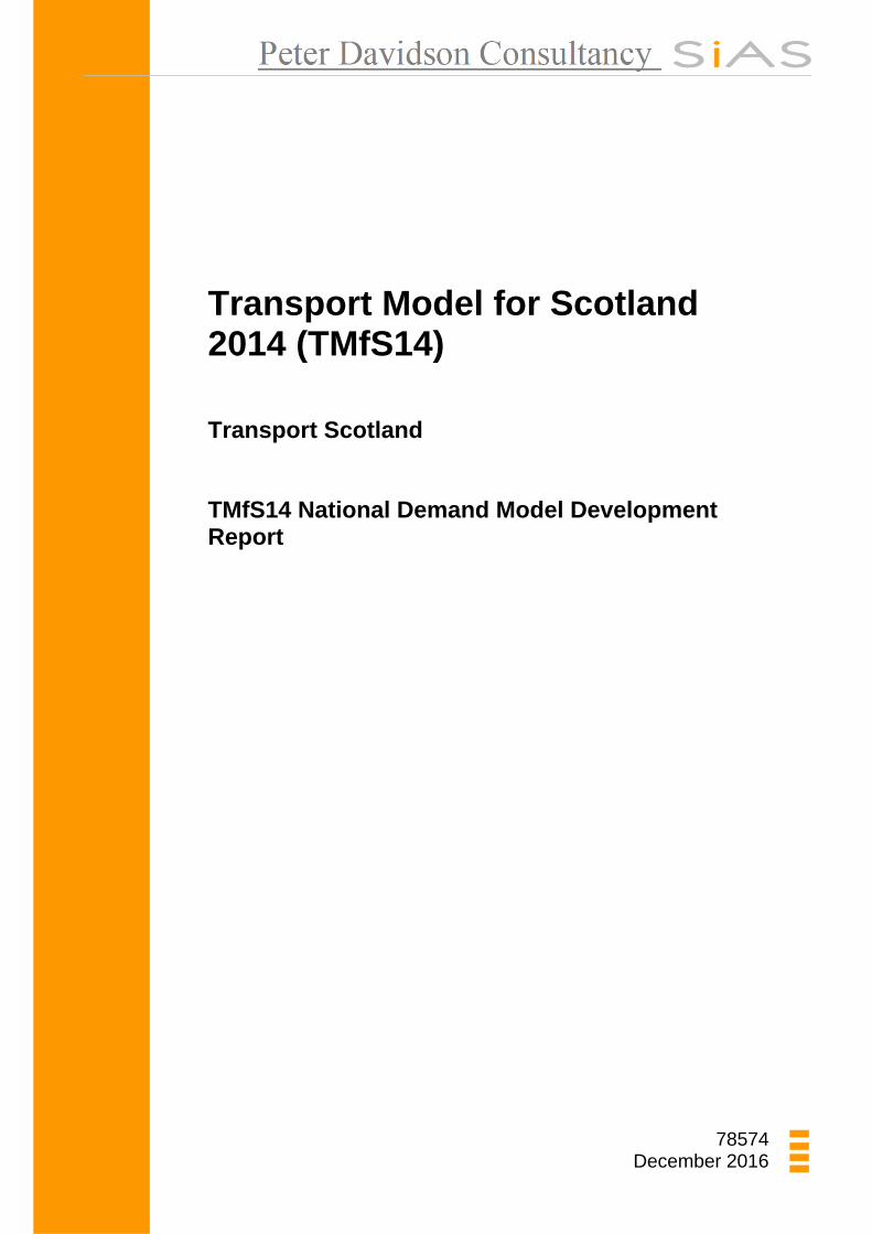
CONTENTS :
Page
1 INTRODUCTION 1
1.1 Background 1 1.2 Introduction 1 1.3 Structure of this Report 3
2 KEY MODEL DIMENSIONS 5
2.1 Introduction 5 2.2 Parking Charges 8
3 MODEL OVERVIEW 9
3.1 Model structure 9 3.2 Initial modal share 11 3.3 Destination choice model 11 3.4 Composite cost calculation 12 3.5 Mode Specific Parameters (MSP) 13 3.6 Mode choice (MC) model 14 3.7 High Occupancy Vehicle choice model 15 3.8 Park & Ride station choice (SC) model 16 3.9 Reverse and non-Home-Based trips model 18 3.10 Assignment prep module 20 3.11 Other choice models 20 3.12 Trip Frequency Model 21 3.13 Macro Time of Day Choice Model 22
4 UPDATING THE BASE YEAR DEMAND MODEL 23
4.1 Introduction 23 4.2 Updating the trip end model base year 23
5 ESTIMATION OF NEW MODE AND DESTINATION CHOICE COEFFICIENTS 25
5.1 Scope of update 25 5.2 Methodology 25 5.3 Sample selection 26 5.4 Utility specification 27 5.5 Resulting coefficients 28 5.6 Calculation of the Final AM Coefficients 29 5.7 Calculation of the Final IP Coefficients 37
6 OTHER UPDATES 47
6.1 New incremental matrices 47 6.2 Park & Ride model update 48
78574
22 December 2016
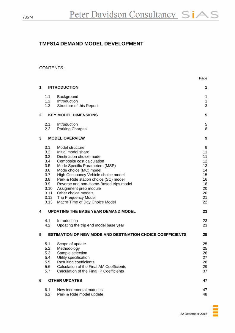
7 SENSITIVITY TESTS 51
7.1 Introduction 51 7.2 Results 51 7.3 Combined Results 52 7.4 AM Elasticities 53 7.5 Inter Peak Elasticities 54
8 FURTHER EXAMINATION OF MODEL RESPONSES 57
8.1 Overall elasticities taken directly after Mode and Destination Choice 57 8.2 AM Elasticities taken directly after Mode and Destination Choice 58 8.3 IP Elasticities taken directly after Mode and Destination Choice 59 8.4 Summary of modelled elasticities 60
9 FORECASTING PROCEDURES 61
9.1 Introduction 61 9.2 Overall Operation of the Demand Model 61 9.3 The Incremental Forecasting Approach 63 9.4 Model Parameters 64 9.5 Road and Public Transport Cost Matrices 64 9.6 Road and Public Transport Networks 64 9.7 Education Matrices 64 9.8 Goods Vehicles 65 9.9 Long Distance Vehicle Matrices 65 9.10 External Trips 65
10 CONCLUSIONS AND RECOMMENDATIONS 67
10.1 Conclusions 67 10.2 Recommendations 67
A PARKING CHARGES 69
B MODEL STRUCTURE 71
C NTEM TRIP RATE ASSUMPTIONS 81
D PARK & RIDE CALIBRATION 83
78574
22 December 2016
TMFS14 DEMAND MODEL DEVELOPMENT
FIGURES :
Page Figure 2.1 : TMfS14 Zone Sector Definition 6
Figure B.1 : Overall Model Architecture 71
Figure B.2 : Main Demand Model Architecture 72
Figure B.3 : Mode & Destination Module 73
Figure B.4 : HOV Model 74
Figure B.5 : Park & Ride Station Choice Model 75
Figure B.6 : Reverse Factoring (Output 1) 76
Figure B.7 : Reverse Factoring (Output 2) 77
Figure B.8 : Reverse Factoring (Output 3) 78
Figure B.9 : Assignment Prep Module 79

78574
22 December 2016
78574
22 December 2016
TMFS14 DEMAND MODEL DEVELOPMENT
TABLES :
Page Table 2.1 : TMfS14 Zone Definition 5
Table 4.1 : Airport Growth Factors 23
Table 5.1 : AM Mode and Destination Choice Coefficients 28
Table 5.2 : Calculation of HBO AM Mode and Destination Choice Coefficients by Car Availability 29
Table 5.3 : Calculation of average AM Home-Based Other Mode and Destination Choice coefficients from 10 estimation runs (Runs 1-4) 30
Table 5.4 : Calculation of average AM Home-Based Other Mode and Destination Choice coefficients from 10 estimation runs (Runs 5-8) 30
Table 5.5 : Calculation of average AM Home-Based Other Mode and Destination Choice coefficients from 10 estimation runs (Runs 9,10 and resulting Average) 31
Table 5.6 : ASCs by Local Authority area used in the AM Other run shown in Table 5.2 to Table 5.5 32
Table 5.7 : Calculation of HBW AM Mode and Destination Choice Coefficients by Car Availability 33
Table 5.8 : Calculation of average AM Home-Based Work coefficient from 10 estimation runs (Runs 1-4) 34
Table 5.9 : Calculation of average AM Home-Based Work coefficient from 10 estimation runs (Runs 5-8) 34
Table 5.10 : Calculation of average AM Home-Based Work coefficient from 10 estimation runs (Runs 9,10 and resulting average) 34
Table 5.11 : Calculation of HBEB AM Mode and Destination Coefficients by Car Availability 35
Table 5.12 : Calculation of average AM Employer’s Business Mode and destination choice coefficients from 10 estimation runs (Runs 1-4) 36
Table 5.13 : Calculation of average AM Employer’s Business Mode and destination choice coefficients from 10 estimation runs (Runs 5-8) 36
Table 5.14 : Calculation of average AM Employer’s Business Mode and destination choice coefficients from 10 estimation runs (Runs 9,10 and resulting Average) 36
Table 5.15 : IP Mode and Destination Choice Coefficients 37
Table 5.16 : Calculation of average IP Home-Based Other Mode and Destination Choice coefficients from 10 estimation runs. 38
Table 5.17 : Calculation of average IP Home-Based Other Mode and Destination Choice coefficients from 10 estimation runs (Runs 1-4) 39
Table 5.18 : Calculation of average IP Home-Based Other Mode and Destination Choice coefficients from 10 estimation runs (Runs 5-8) 39
Table 5.19 : Calculation of average IP Home-Based Other Mode and Destination Choice coefficients from 10 estimation runs (Runs 9, 10 and resulting Average) 39
78574
22 December 2016
Table 5.20 : ASCs by Local Authority area used in the IP Other run shown in Table 5.16 to Table 5.19 40
Table 5.21 : Calculation of average IP Home-Based Work coefficient from 10 estimation runs 41
Table 5.22 : Calculation of average IP Home-Based Work Mode and Destination Choice coefficients from 10 estimation runs (Runs 1-4) 42
Table 5.23 : Calculation of average IP Home-Based Work Mode and Destination Choice coefficients from 10 estimation runs (Runs 5-8) 42
Table 5.24 : Calculation of average IP Home-Based Work Mode and Destination Choice coefficients from 10 estimation runs (Runs 9, 10 and resulting Average) 42
Table 5.25 : Calculation of HBEB IP Coefficients by Car Availability 43
Table 5.26 : Calculation of average IP Employer’s Business Mode and Destination Choice coefficients from 10 estimation runs (Runs 1-4) 44
Table 5.27 : Calculation of average IP Employer’s Business Mode and Destination Choice coefficients from 10 estimation runs (Runs 5-8) 44
Table 5.28 : Calculation of average IP Employer’s Business Mode and Destination Choice coefficients from 10 estimation runs (Runs 9, 10 and resulting average) 44
Table 6.1 : Park and Rite Site Calibration by Local Authority 49
Table 7.1 : WebTAG Elasticity Ranges (Table 6.2, TAG Unit M2, January 2014) 52
Table 7.2 : Calculated TMfS14 Elasticity Ranges 52
Table 7.3 : AM Peak Fuel Sensitivity Test Elasticities by location 53
Table 7.4 : AM Peak Car Journey Time Elasticities by location 53
Table 7.5 : AM Peak Public Transport Fare Demand Elasticities by location 53
Table 7.6 : Inter Peak Fuel Sensitivity Test Elasticities by location 54
Table 7.7 : Inter Peak Car Journey Time Elasticities by location 54
Table 7.8 : Inter Peak Public Transport Fare Demand Elasticities by location 55
Table 8.1 : Combined Purpose Elasticities by Journey Type and location 57
Table 8.2 : AM Peak Fuel Sensitivities, taken directly after Mode and Destination Choice by location 58
Table 8.3 : AM Peak Car Journey Time Elasticities, taken directly after Mode and Destination Choice. by location 58
Table 8.4 : AM Peak Public Transport Fare Demand Elasticities, taken directly after Mode and Destination Choice by location 58
Table 8.5 : Inter Peak Fuel Sensitivity Test, taken directly after Mode and Destination Choice by location 59
Table 8.6 : Inter Peak Car Journey Time Elasticities, taken directly after Mode and Destination Choice by location 59
Table 8.7 : Inter Peak Public Transport Fare Demand Elasticities, taken directly after Mode and Destination Choice by location 59
Table A.1 : Destination zones where parking zones are applied 69
Table A.2 : Average Charges (£) 69
Table A.3 : Parking Charges as a Generalised Cost (Mins) 69
Table D.1 : Park & Ride by Local Authority 84
Table D.2 : Park & Ride by Local Authority (Cont.) 85

78574
22 December 2016
Table D.3 : Park & Ride by Local Authority (Cont.) 86
Table D.4 : Park & Ride by Local Authority (Cont.) 87
Table D.5 : Park & Ride by Local Authority (Cont.) 88
Table D.6 : Park & Ride Calibration by site (Vehs) 89
Table D.7 : Park & Ride Calibration by site (Vehs) (Cont.) 90
Table D.8 : Park & Ride Calibration by site (Vehs) (Cont.) 91
Table D.9 : Park & Ride Calibration by site (Vehs) (Cont.) 92

78574
22 December 2016
78574
Page 1 of 92 22 December 2016
1 INTRODUCTION
1.1 Background
Transport Scotland plays a key role in the assessment of proposed changes to land use and transport networks across Scotland. As part of the planning process, Transport Scotland offers the use of its strategic transport and land use appraisal tools to assess the social, economic, operational, and environmental impacts of different land use options and transport interventions.
These appraisal tools include National integrated land use and transport models which cover the whole of Scotland. These National models include both the Transport Model for Scotland (TMfS) and the Transport, Economic, and Land-use Model of Scotland (TELMoS) which are both developed and maintained under Transport Scotland’s Land Use and Transport Integration in Scotland service (LATIS).
For more information regarding the LATIS service and the National Transport and Land Use Models, please visit the LATIS website: www.transportscotland.gov.uk/latis
Transport Scotland requested the development of TMfS14 which is calibrated to transport and land use conditions observed during 2014, with this model being an update of the previous TMfS12. The TMfS14 development was to consider:
During the development of TMfS12 a number of additional data sources became available or were identified as missing, technical challenges were encountered, enhancements proposed and other models developed.
TMfS shall incorporate the new data, technical updates and potentially the proposed enhancements. This model shall also have the specific objective of being suitable for supporting the Outline Business Case for improvements on the Inverness to Aberdeen transport corridor.
This model is to be used to prepare a single (baseline) Forecast Scenario for the future years; 2017 – 2037 at five year intervals.
1.2 Introduction
In summer 2012 SIAS Limited (SIAS) was appointed as a nominated consultant within the Multiple Framework Agreement (MFA) for the Transport Planning, Modelling and Audit Services, Lot 1: Commission for the Maintenance and Enhancement of TMfS, which encompasses the maintenance and enhancement of the existing LATIS models.
The Transport Model for Scotland (TMfS12) was a “light touch” refresh of TMfS07 to 2012 conditions undertaken by SIAS throughout the first half of 2013. TMfS12 and its associated primary forecasts were circulated to all LATIS Framework Participants in the summer of 2013 for use on various applications. The primary focus of TMfS12 was its future application on the A9 Dualling between Perth and Inverness and therefore any updates to the model will also apply to this corridor.
In December 2014 SIAS provided Transport Scotland with an updated programme for the development of TMfS12A, an updated version of TMfS12 utilising the 2011 census travel to work data which had become available from the National Records for Scotland. Following this, Transport Scotland agreed that the demand model structure needs to change to include the ports and other zone disaggregation opportunities would also be included to take advantage of this change to the demand model.
78574
Page 2 of 92 22 December 2016
Further TMfS12A scoping discussions took place which concluded on 28 May 2015, where Transport Scotland (TS) requested that SIAS and Peter Davidson Consultancy Limited (PDC) update TMfS12 to create TMfS14. The scope of this commission contains the following elements (SIAS Ref. 78104,TMfS14 Specification Note, June 2016):
Updating TMfS12 to a 2014 base year, thus creating TMfS14
Establishing TMfS14/TELMoS14 requirements and features
Incorporating 2011 census travel to work data
Data collection, collation and assimilation
Homogenising the zone system between the demand and assignment models
Establishing a range of forecast scenarios for TMfS14/TELMoS14
Calibration, validation and realism testing of the demand model
Calibration and validation of the road and PT assignment models
Updating the TMfS14 Trip End Model
Preparing a release version of TMfS114
Engagement with the LATIS Lot 3 participant David Simmonds Consultancy (Development, Update and Application of the Transport Economic Land-Use Model of Scotland (TELMoS)
Preparation of updated technical and support documentation
The key changes to the TMfS14 demand model were as shown as follows:
Additional Park & Ride sites added to the model
Updated base year trip ends, re-basing the trip end model to a 2014 base year
Mode and destination choice models re-estimated using household travel survey data and the observed matrices
Updated vehicle occupancy inputs for 2014
New incremental matrices to compensate for differences between the validated matrices and the synthesized base matrices
Elasticity calculations for realism testing
This Report covers work undertaken to update the demand model from 2012 to 2014 base year. References in this Report to the Demand Model and Model refer to the 2014 update. If the previous TMfS07 or TMfS12 models are referred to it will be made clear in the text.

78574
Page 3 of 92 22 December 2016
This Report describes the development, calibration, and validation of the TMfS14 National Road Model and is one of a series of documents describing the development, calibration, and validation of the TMfS14 models, as follows:
TMfS14 National Road Model Development Report
TMfS14 National Public Transport Model Development Report
TMfS14 Demand Model Development Report
TMfS14 Forecasting Report
1.3 Structure of this Report
The structure of the remainder of this Report is as follows:
Section 2 Key model dimensions
Section 3 Model overview
Section 4 Updating the base year demand model
Section 5 Estimation of mode and destination choice coefficients
Section 6 Other updates
Section 7 Sensitivity tests
Section 8 Further examination of model responses
Section 9 Forecasting procedures
Section 10 Conclusions and recommendations.

78574
Page 4 of 92 22 December 2016
78574
Page 5 of 92 22 December 2016
2 KEY MODEL DIMENSIONS
2.1 Introduction
The main inputs to the TMfS14 Demand Model were:
Updated trip ends from the trip end model
2014 demographic data from TELMOS
New base year generalised cost matrices for Road and public transport modes
Road and public transport networks
Park & ride site files
Validated base year trip matrices for the three main car journey purposes described below and for goods vehicles
Incremental matrices
Model parameters
The TMfS14 Model has a revised zone system with 799 zones. The additional zones are created by splitting some of the old zones into two or more new zones, thus allowing a clear correspondence to be developed between the two. The new zone system, as shown in Table 2.1, consists of:
779 internal zones; Zones 1 – 708 and 713 – 783
4 airport zones (Aberdeen, Edinburgh, Glasgow and Prestwick); Zones 709 – 712
16 external zones covering England and Wales; Zones 784 – 799
This change provides additional spatial detail and also ensures that all but one zone contains no more than one rail station per zone.
Table 2.1 : TMfS14 Zone Definition
TMfS12 TMfS14
Internal zones 708 779Airport zones 4 4External zones 8 16Total 720 799
78574
Page 6 of 92 22 December 2016
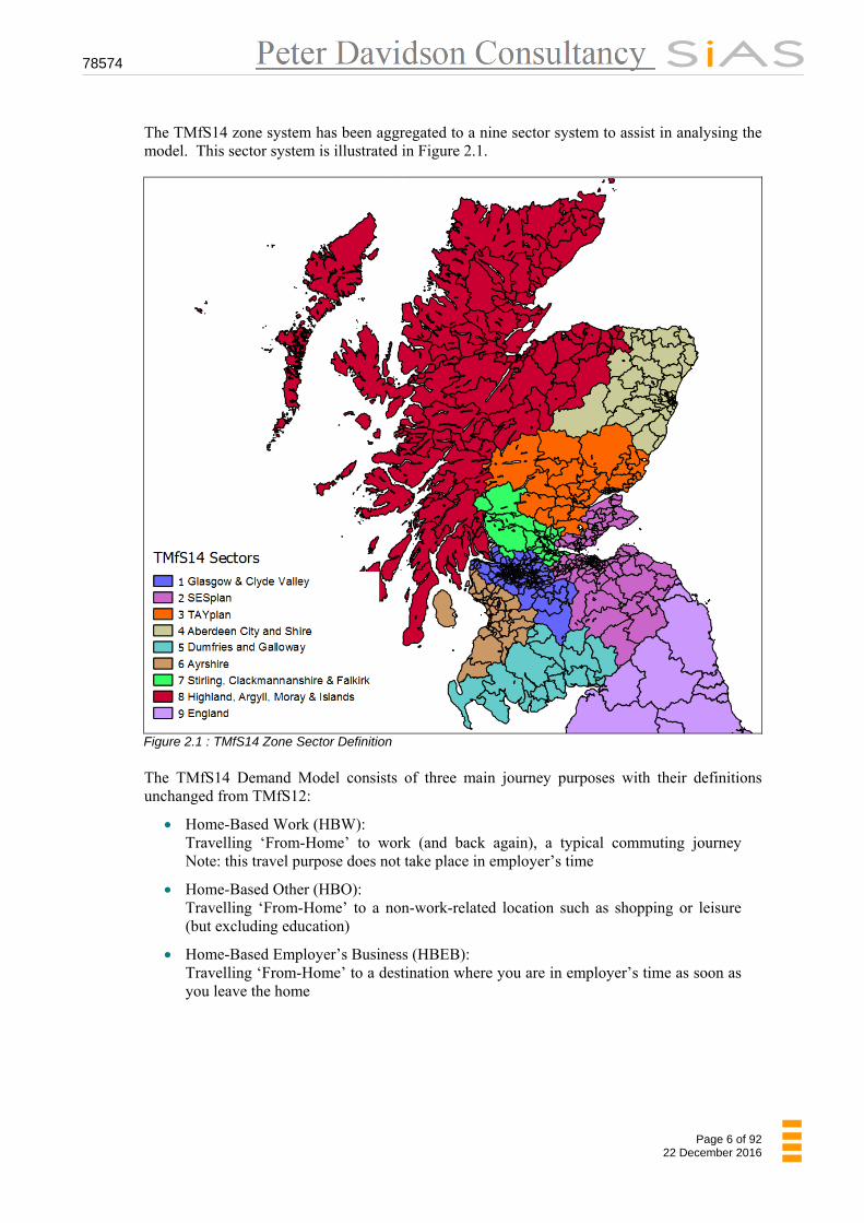
The TMfS14 zone system has been aggregated to a nine sector system to assist in analysing the model. This sector system is illustrated in Figure 2.1.
Figure 2.1 : TMfS14 Zone Sector Definition
The TMfS14 Demand Model consists of three main journey purposes with their definitions unchanged from TMfS12:
Home-Based Work (HBW): Travelling ‘From-Home’ to work (and back again), a typical commuting journey Note: this travel purpose does not take place in employer’s time
Home-Based Other (HBO): Travelling ‘From-Home’ to a non-work-related location such as shopping or leisure (but excluding education)
Home-Based Employer’s Business (HBEB): Travelling ‘From-Home’ to a destination where you are in employer’s time as soon as you leave the home
78574
Page 7 of 92 22 December 2016
Three other journey purposes complement the above main purposes:
Non-Home-Based Other (NHBO): Travelling between two Non-Home-Based locations (e.g. from work to shop)
Non-Home-Based Employer's Business (NHBEB): Travelling during employer’s time, such as travel from place of work to a business meeting, visiting customers, etc.
Home-Based Education (HBS): Travelling ‘From-Home’ to an education destination (e.g. school, university, etc.).
These latter three purposes are not part of the main Demand Model, but are added separately after the mode and destination choice process, as part of the reverse factoring sub application.
Each journey purpose is segmented into four household types:
C0 Zero car households (everyone from these is considered to be captive to PT)
C1/1 1 car, 1 adult household
C1/2+ 1 car, 2+adult household
C2+ 2+ car household
Three main modes are considered in the Demand Model:
Car
Public transport (PT)
Park & Ride
Separate demand models were developed for the morning peak (AM) and inter peak (IP) periods. Evening peak demand is extracted from the demand for the other time periods. The periods are defined as:
AM Peak period 07:00 – 10:00
AM peak hour (for assignment modelling) 08:00 – 09:00
Inter peak period 10:00 – 16:00
Inter peak hour (for assignment modelling) 1/6 of 10:00 – 16:00
PM peak period 16:00 – 19:00
PM peak hour (for assignment modelling) 17:00 – 18:00

78574
Page 8 of 92 22 December 2016
Five user classes were used in the Road assignment supply model:
Car in work time
Car in commute time
Cars in other time (shopping, leisure, etc.)
Light goods vehicles (LGV)
Heavy goods vehicles (HGV)
Each of these user classes has a separate set of weightings for distance and time, affecting the routeing that the Cube model calculates. These weightings also change across the modelled years.
The PT assignment assigns three user classes:
PT in work time
PT in commute time
PT in other time (shopping, leisure, etc.)
Through the PT factor files (applied in route enumeration process) two different values of time are applied; one for travel in work time, and a separate, lower value for commute and other purposes.
2.2 Parking Charges
Parking charges are introduced by adding representative costs to the central area zones of:
Aberdeen
Dundee
Dunfermline
Edinburgh
Glasgow
Inverness
Perth
Stirling
Different costs are added in for different journey purposes. This is due to different types of journey having different average lengths of stay.
Appendix A describes how the parking charges have been included in the Model. It also describes the calculation of average parking charges in each city/town.
78574
Page 9 of 92 22 December 2016
3 MODEL OVERVIEW
This section describes the model, based on reviewing the available documentation, Cube model, and code. Where appropriate, formulae have been included within the text and flow diagrams illustrating the processes have been presented in Appendix B.
3.1 Model structure
The TMfS14 Model is an extension of the conventional “four-stage” model, and incorporates the stages/choices listed as follows:
Trip Generation Model
Trip Frequency
Macro Time of the Day Model
Main Demand Module
Assignment Models
The Macro time of the day and the Trip Frequency models are switched off by default in the TMfS07, TMfS12, and TMfS14 models. They have not been run in TMfS14, although the code has been checked to ensure that it is compatible with the updated model.
The Macro time of the day and the Trip Frequency models are turned off in the TMfS07, TMfS12, and TMfS14 models.
The Mode and Destination Choice Module forms the main choice mechanism within the TMfS14 model.
The Main Demand Module (shown in Appendix B, Figure 2) consists of the following sub-models:
Mode and Destination Choice Module
High Occupancy Vehicle (HOV) Choice Model
Park & Ride Station Choice Model
Long Distance Model
Reverse Factoring and Non-Home-Based Module
Assignment Preparation Module
The High Occupancy Vehicle Choice model is switched off by default and has not been tested in TMfS14. As with the Trip Frequency Model, the code has been checked to ensure that it is compatible with the updated model.
Appendix B, Figure 3 shows the structure of the Mode and Destination module and how the sub-models are connected. This module first executes the Initial Mode Choice Model (IMC) to produce initial trip ends by mode. The Destination Choice Model (DM) then distributes the trip ends for each mode to all available destination zones using a traditional gravity model. At this stage trip matrices for the three modes are produced.
For each mode and household type the composite cost of travel from each origin zone was calculated using a formulation similar to the traditional logsum.
78574
Page 10 of 92 22 December 2016
i ijmhmhijmhmhmh
ijmh
iijmh CCIntrazonal
TripsTrips
210 lnexplnln
These logsums are used to update the mode specific constants using the Mode Specific Parameters (MSP) module (on the first iteration). Finally, the modal share is updated using the Mode Choice (MC) model using the logsums and the mode specific constants as inputs. These updated mode shares are then used to update the trip matrices using the Distribution Model (DC), the logsums, and then the mode specific constants.
The resulting trip matrices by mode produced from the Mode & Destination choice module are ‘From-Home’ AM and IP trip matrices for the three main purposes (Home-Based Work, Home-Based Employers Business, and Home-Based Other). At this stage, if the HOV model had been turned on, it would have split the trips between each origin-destination pair for each mode and time period into High Occupancy Vehicle (HOV) trips and Single Occupancy Vehicle (SOV) trips. The Park & Ride trip matrices are then used as input by the Park & Ride Station Choice model to produce parking demand at each parking site.
The next stage produces evening peak (PM) ‘From-Home’ matrices from the IP ‘From-Home’ matrices using observed PM to IP factors. The resulting AM, IP, and PM ‘From-Home’ matrices are then used to create ‘To-Home’ AM, IP, and PM matrices. Finally, Non-Home-Based trip ends and trip matrices are derived from these matrices. All these processes are created by the Reverse Factoring module.
The final stage of the demand model involves preparing matrices for Road assignment using the Assignment Prep Module. At this stage external, long distance, and Education matrices, together with vehicle occupancy factors and period to hour factors are added to create five different user classes for Road assignment, and three user classes for PT assignment:
Road user classes:
Car in work time
Car in commute time
Car in other time
Light Goods Vehicles (LGV)
Heavy Goods Vehicles (HGV)
PT user classes:
PT in work time
PT in commute time
PT in other time
The final synthesised matrices, by Car user and PT user classes, are then ‘corrected’ with respect to the difference between the synthetic and validated (observed) base-year matrices using incremental matrices before assigning them.
The assignments generate a new set of cost matrices which go through the Generalised Cost Calculations module and are then fed back into the demand model to produce a new set of matrices. This demand-supply loop continues until convergence or a pre-defined number of iterations has been performed.
78574
Page 11 of 92 22 December 2016
3.2 Initial modal share
The first time round the main demand-supply loop, the model uses a starting mode split between car and PT which comes in through the trip ends from the trip end model. The Park & Ride trips are then split out from the PT trip ends using a set of factors files. Later in this first iteration, and in subsequent iterations, the mode share will be recalculated as a function of the generalised costs and the mode specific parameters.
3.3 Destination choice model
The destination choice model for ‘From-Home’ purposes, uses the following inputs:
Trip productions for car and public transport by each car availability segment
Trip attractions/attraction factors for all modes and car availability types combined
Generalised costs of travel by car and by Public Transport
These inputs are used to create matrices of person trips, separately by time period and trip purpose, for ‘From-Home’ trips. This process is carried out at a zonal level.
The process is a traditional gravity model process applied in a doubly constrained manner for ‘From-Home’ commute trips, and singly constrained for other ‘From-Home’ purposes. There are separate sensitivity parameters for each trip purpose/mode/household-type combination.
The spread parameters are β1, and β2. There are also Intra-Zonal factors β0, which affect the number of intra-zonal trips produced.
The outputs of this process are person trip matrices by time period, trip purpose/mode/car availability.
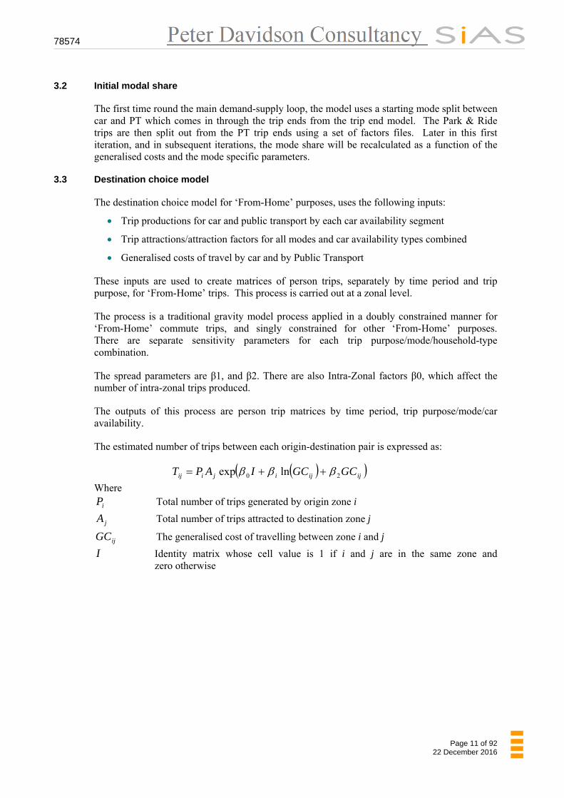
The estimated number of trips between each origin-destination pair is expressed as:
ijijijiij GCGCIAPT 20 lnexp
Where
iP Total number of trips generated by origin zone i
jA Total number of trips attracted to destination zone j
ijGC The generalised cost of travelling between zone i and j
I Identity matrix whose cell value is 1 if i and j are in the same zone and zero otherwise
78574
Page 12 of 92 22 December 2016
3.4 Composite cost calculation
This process follows the distribution model processes and calculates the logsum used in the mode choice process.
The matrices generated by the destination choice model along with the generalised costs by mode, as used in the destination choice model, are used to calculate a trip weighted composite cost for each origin zone.
The process was conducted separately for each ‘From-Home’ trip purpose and Car Available segment. For the Non-Car Available segments there is no mode choice, but the utilities are still calculated and input to the time of day choice and trip frequency choice processes. In the case of Car Available, the output utilities are used as input to the mode choice, time of day choice, and trip frequency choice processes.
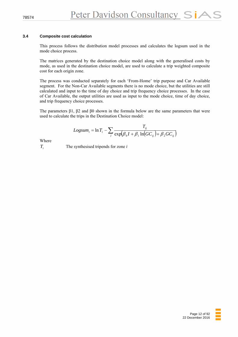
The parameters β1, β2 and β0 shown in the formula below are the same parameters that were used to calculate the trips in the Destination Choice model:
j ijij
ijii GCGCI
TTLogsum
210 lnexpln
Where
iT The synthesised tripends for zone i

78574
Page 13 of 92 22 December 2016
3.5 Mode Specific Parameters (MSP)
The forecast trip ends provided by the trip end model are the forecast trip ends based on base year costs, in other words they forecast future travel demand by zone and by mode based on demographic changes but assuming no change in travel costs from the base year.
When the model is run for future years, the demand model includes a process that calculates the MSPs so that they reproduce the forecast trip ends with base year costs. When the model is run for future years, the model initially creates the reference case Road and PT matrices for the year in question. These reference case matrices reflect expected land-use and car ownership changes (through the outputs provided by the trip end model) but take no account of cost changes.
As per TAG unit M2 2.5.12, which describes the reference case forecast as follows:
The construction of the reference case forecast requires reference case growth factors/assumptions and will involve the adjustment of the row and column of the base P/A matrix at an all-day all-modes level to reflect expected land-use and car ownership changes (taking no account of cost changes). As a default, these should be based on NTEM.
The MSPs are calculated to ensure that when the demand model produces its first set of matrices (which use the base year costs), these matrices reproduce the mode shares given by the future year trip ends that came out of the trip end model. The mode split is then allowed to vary according to the changing generalised costs in the future year scenario.
So, the mode specific constants, (or K,) are calculated for each zone using the formulae given. This calculation is only carried out on the first iteration of the supply-demand loop and uses the generalised costs from the base year.
These matrices are then assigned to the future year Road and PT networks, and the generalised costs are calculated. The costs are then fed back in to the demand model for the second and subsequent iterations of the outer supply-demand loop and the modelled responses will then change on the basis of the differences between base year costs and forecast year costs.
Subsequent iterations, which will return a new set of generalised costs, will then use these MSP together with the new generalised costs to calculate the mode split in the mode choice model.
)(
)()()()(
)(
)()()()(
ln1
ln1
PnRi
PTiPTiPnRiPTi
PnRi
CariCariPnRiCari
P
PLsumLsumK
P
PLsumLsumK
Where
)(CariP Proportion of car trips generated from zone i in the base year
Mode choice scaling factor Lsum Logsum or composite utility
These formulae were derived from the mode split formulation and are calculated for each journey purpose.
Note that they are relative to the Park & Ride Mode Constant ,which is set to zero.
78574
Page 14 of 92 22 December 2016
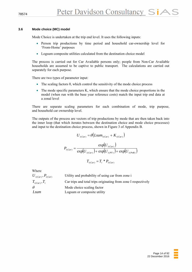
3.6 Mode choice (MC) model
Mode Choice is undertaken at the trip end level. It uses the following inputs:
Person trip productions by time period and household car-ownership level for ‘From-Home’ purposes
Logsum composite utilities calculated from the destination choice model
The process is carried out for Car Available persons only; people from Non-Car Available households are assumed to be captive to public transport. The calculations are carried out separately for each purpose.
There are two types of parameter input:
The scaling factors θ, which control the sensitivity of the mode choice process
The mode specific parameters K, which ensure that the mode choice proportions in the model (when run with the base year reference costs) match the input trip end data at a zonal level
There are separate scaling parameters for each combination of mode, trip purpose, and household car ownership level.
The outputs of the process are vectors of trip productions by mode that are then taken back into the inner loop (that which iterates between the destination choice and mode choice processes) and input to the destination choice process, shown in Figure 3 of Appendix B.
)()()( CariCariCari KLsumU
)()()(
)()( expexpexp
exp
PnRiPTiCari
CariCari UUU
UP
)()( * CariiCari PTT
Where
)()( , CariCari PU Utility and probability of using car from zone i
iCari TT ,)( Car trips and total trips originating from zone I respectively
Mode choice scaling factor Lsum Logsum or composite utility

78574
Page 15 of 92 22 December 2016
3.7 High Occupancy Vehicle choice model
If switched on, this model is executed after the mode and destination loop. The High Occupancy Vehicle (HOV) choice Model allows trips to move between single occupancy vehicles and multiple occupancy vehicles.
Note that the HOV choice is ‘off’ by default, so will not split the trips into single and high occupancy trip matrices at the time of writing.
The Module sits after the Inner Loops procedure, which loops over mode choice and destination choice within the Model structure, before the Park & Ride (P&R) station choice and reverse factoring applications. It works on the Home-Based Work, Home-Based Employers Business trips, and Home-Based Other trips for the household segments C1/1, C1/2+ and C2+.
The occupancy choice takes the form of a logit model using different generalised costs for Single Occupancy and High Occupancy trips. The person trip proportion of low occupancy for a particular ij pair will be:
HOSO
SOSO GCGC
GCP
expexp
exp
Where
HOSO GCGC , Generalised cost for low and high occupancy respectively
Is a high occupancy penalty for representing additional travel and difficulty in arranging passengers
Is a sensitivity parameter of the logit model
The output of this is ‘From-Home’ matrices by purpose and segment for High Occupancy and Single Occupancy. These are then passed through the reverse trip process and converted into vehicle OD matrices using occupancy factors.
Finally, Road Assignment and Public Transport Assignment are undertaken. If there are specific High Occupancy Vehicle lanes, they need to be coded into the Model as a separate link type (the Road Model has link types for HOV only and HOV and HGV). The High Occupancy and Single Occupancy costs are then skimmed separately to be put back into the Demand Model.

78574
Page 16 of 92 22 December 2016
3.8 Park & Ride station choice (SC) model
The Park & Ride Station Choice model follows the High Occupancy Vehicle Choice Model. It is applied to ‘Car Available’ trips ‘From-Home’ (produced by the Destination Choice Model) in the AM Peak Period only. The corresponding return trips are assumed to take place during the PM Peak period.
The inputs to the Station Choice model were:
Park & Ride generalised cost.
Park & Ride trip matrices. (From the Mode & Destination Choice models)
Park & Ride Sites and their attributes. The attributes included Car Park charge (if any), the number of ‘official’ car parking spaces, and transfer times.
A single parameter, the calibrated transfer time attribute of each car park, aims to reflect a variety of attributes of the Park & Ride site (e.g. cleanliness, ease of transfer, and security) and was used as a calibration tool. This parameter does not vary with car occupancy, however, there is also an element of cost which does vary according to the demand for the site, also referred to as the transfer time.
The model operates in an iterative fashion. The process initially split the Park & Ride trips between each Origin-Destination pair across the available car parks using generalised cost; car park cost and the calibrated transfer time.
Sites that are over capacity have their associated transfer times increased as a function of the modelled demand and capacity at that site. This is to represent the increasing search and/or walk time associated with using the non ‘official’ car parking spaces.
The generalised costs were calculated from combinations of the Road and PT costs. Park & Ride cost matrices are the best path cost matrices. They are built by finding the minimum path from each origin to each Park & Ride site by car and then from there to each destination.

78574
Page 17 of 92 22 December 2016
Park & Ride trips calculated from the Mode and Destination choice models are assigned to the Park & Ride sites using the logit formula:
)( )()()()( SSijSijSij PCTTGCU
Sssij
sijsij U
UP
)(
)()( exp
exp
)()( * sijijsij PTT
ji
sijs TT,
)(
Where
)(sijGC Generalised cost of using car park s between each OD pair
)(sijTT Transfer time of using car park s between each OD pair
sPC Parking cost for car park s
Spread parameter for the park and ride station choice
The Park & Ride model works separately for each of the three main purposes. It calculates the Home-Based Work, Home-Based Employers Business and Home-Based Other trips simultaneously. The output is by site for each of the above purposes.
External trips (i.e. trips from England and Wales) do not have the choice of using Park & Ride as they are not included in the mode choice calculations. The Park & Ride model outputs AM ‘From-Home’ and PM ‘To-Home’ matrices by purpose and mode. These were added into the Road and PT assignment matrices before assignment.
78574
Page 18 of 92 22 December 2016
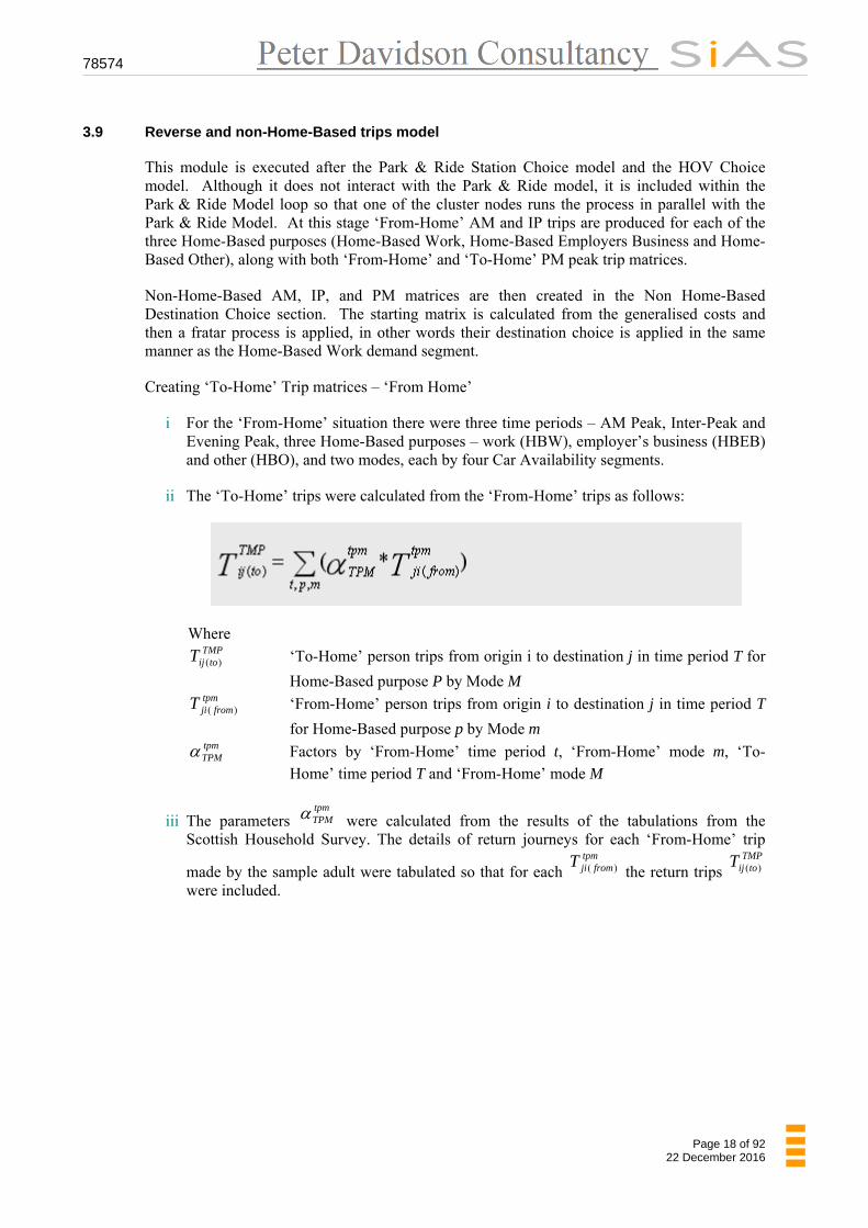
3.9 Reverse and non-Home-Based trips model
This module is executed after the Park & Ride Station Choice model and the HOV Choice model. Although it does not interact with the Park & Ride model, it is included within the Park & Ride Model loop so that one of the cluster nodes runs the process in parallel with the Park & Ride Model. At this stage ‘From-Home’ AM and IP trips are produced for each of the three Home-Based purposes (Home-Based Work, Home-Based Employers Business and Home-Based Other), along with both ‘From-Home’ and ‘To-Home’ PM peak trip matrices.
Non-Home-Based AM, IP, and PM matrices are then created in the Non Home-Based Destination Choice section. The starting matrix is calculated from the generalised costs and then a fratar process is applied, in other words their destination choice is applied in the same manner as the Home-Based Work demand segment.
Creating ‘To-Home’ Trip matrices – ‘From Home’
i For the ‘From-Home’ situation there were three time periods – AM Peak, Inter-Peak and Evening Peak, three Home-Based purposes – work (HBW), employer’s business (HBEB) and other (HBO), and two modes, each by four Car Availability segments.
ii The ‘To-Home’ trips were calculated from the ‘From-Home’ trips as follows:
Where TMP
toijT )( ‘To-Home’ person trips from origin i to destination j in time period T for
Home-Based purpose P by Mode M tpm
fromjiT )( ‘From-Home’ person trips from origin i to destination j in time period T
for Home-Based purpose p by Mode m tpmTPM Factors by ‘From-Home’ time period t, ‘From-Home’ mode m, ‘To-
Home’ time period T and ‘From-Home’ mode M
iii The parameters tpmTPM were calculated from the results of the tabulations from the
Scottish Household Survey. The details of return journeys for each ‘From-Home’ trip
made by the sample adult were tabulated so that for each tpm
fromjiT )( the return trips TMP
toijT )( were included.

78574
Page 19 of 92 22 December 2016
Creating ‘To-Home’ Trip matrices - 'Non-Home-Based'
i For Non-Home-Based trips, the origins and destinations for the two Non-Home-Based purposes (In-Work and Non-Work) were calculated based on the destinations of ‘From-Home’ trips and the origins of ‘To-Home’ trips. The Non-Home-Based, trip ends were calculated separately by time period
ii The Non-Home-Based origin trip ends were derived as follows:
pt
tpmtoj
ntpmtoj
ni DO )()( *
Where n is the Non Home-Based purpose (i.e. Employers business and Other)
Note that the factors β are zero for time periods later than the Non-Home-Based origins/destinations
iii It is unlikely that the total origins would equal the total destinations when applying this process, so the totals were constrained to an average of the two. Matrices of Non-Home-Based trips by mode and time period were created by applying the trip ends to a distribution model using appropriate inter-zonal costs
iv The total trips by mode were calculated simply by adding the origin destination matrices together for Public Transport, and weighting by vehicle occupancy for car trips.
v Once the trip ends for the Non-Home-Based purposes were computed they were distributed to the available destination zones using the ‘Fratar’ method.

78574
Page 20 of 92 22 December 2016
3.10 Assignment prep module
This module combines the matrices produced by the demand model with add-in matrices (such as education, long distance, and external trip matrices) and factors such as occupancy factors, period to hour factors, etc. to produce five user classes for Road assignment:
Cars in work time
Cars in commute time
Cars in other time (e.g. shopping and leisure)
Light Goods vehicles (LGV)
Heavy goods vehicles (HGV)
The module also produces three user classes for PT assignment:
PT in work-time
PT in commute-time
PT in other-time
The resulting matrices are then ‘pivoted’ using the incremental matrices before assignment.
3.11 Other choice models
These include the Trip Frequency Model, and the Macro Time of Day Model. They form part of the demand model and can be switched on or off by the user. They are switched off by default in TMfS07, TMfS12, and the current TMfS14.
78574
Page 21 of 92 22 December 2016
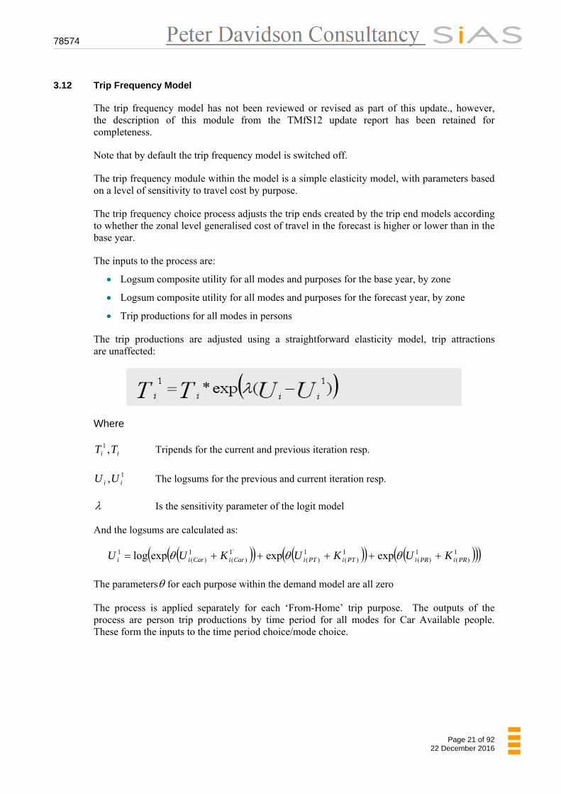
3.12 Trip Frequency Model
The trip frequency model has not been reviewed or revised as part of this update., however, the description of this module from the TMfS12 update report has been retained for completeness.
Note that by default the trip frequency model is switched off.
The trip frequency module within the model is a simple elasticity model, with parameters based on a level of sensitivity to travel cost by purpose.
The trip frequency choice process adjusts the trip ends created by the trip end models according to whether the zonal level generalised cost of travel in the forecast is higher or lower than in the base year.
The inputs to the process are:
Logsum composite utility for all modes and purposes for the base year, by zone
Logsum composite utility for all modes and purposes for the forecast year, by zone
Trip productions for all modes in persons
The trip productions are adjusted using a straightforward elasticity model, trip attractions are unaffected:
Where
ii TT ,1 Tripends for the current and previous iteration resp.
1, ii UU The logsums for the previous and current iteration resp.
Is the sensitivity parameter of the logit model
And the logsums are calculated as:
1)(
1)(
1)(
1)(
`1)(
1)(
1 expexpexplog PRiPRiPTiPTiCariCarii KUKUKUU
The parameters for each purpose within the demand model are all zero
The process is applied separately for each ‘From-Home’ trip purpose. The outputs of the process are person trip productions by time period for all modes for Car Available people. These form the inputs to the time period choice/mode choice.

78574
Page 22 of 92 22 December 2016
3.13 Macro Time of Day Choice Model
The Macro Time of Day Choice Model has not been reviewed or revised as part of this update, however, the description of this module from the TMfS12 update report has been retained for completeness.
The Macro Time of Day Choice is applied to the AM ‘From-Home’ Trip Ends.
Note that it is switched off by default.
The time of day choice module takes as inputs logsum composite costs and trip ends (as amended by the trip frequency module if it is turned on). It is an incremental logit model, which compares the base and the forecast logsum utilities to amend the proportions of travellers in each time period.
Time of Day choice outputs are trip ends by each Car Availability segment, which then go into the main demand model.
1)(
1)(
1)(
1)(
)(1
)(expexp1
1
AMiPREiAMiIPi
PMIPAMiAMiKUBUUA
TT
Where
ii TT ,1 Tripends for the current and previous iteration respectively
ii UU ,1 The logsums for the current and previous iteration respectively
Is the sensitivity parameter of the logit model
And
)(
)(
)(
)( ,AMi
PREi
AMi
IPi
T
TB
T
TA
PRE’ in a subscript in the equations above refers to the pre-peak period.
78574
Page 23 of 92 22 December 2016
4 UPDATING THE BASE YEAR DEMAND MODEL
4.1 Introduction
Several updates were carried out within the changes for TMfS14. Among these: the model zone system was updated from 720 to 799 zones, the P&R model was updated to include additional sites, the base year trip end model was rebased to 2014 and adjusted to work with new data formats, mode and destination choice models were re-estimated and the incremental matrices were updated.
Further detail on the trip end model, mode and destination choice re-estimation and incremental matrices is provided as follows. This Report then goes on to describe the realism testing that was carried out with the updated model.
The Park & Ride was found not to converge and the base transfer time parameters and other aspects were adjusted to improve this.
4.2 Updating the trip end model base year
The trip end model was rebased to 2014. With the zone system extended from 720 zones in TMfS12 to 799 zones in TMfS14, the trip end model was also updated to use inputs and produce outputs with 799 zones.
The trip rates applied were also updated to use the NTEM 6.2 dataset and were applied by area type, although it was found that in practice the specific elements extracted from the NTEM dataset for use in TMfS14 had not changed from those applied in TMfS12.
Previous versions of TMfS applied the NTEM trip rates for a single area type to all model zones. TMfS14 applied the different rates according to the NTEM area types for model zones. This means that rather than assuming that all of the modelled zones related to one of NTEM’s area types, each zone was assigned a different area type which allowed the trip end model to reflect differences in trip making between suburban and rural zones. Future year forecasts assume that the area types remain the same as in the base. Further details are provided in Appendix C.
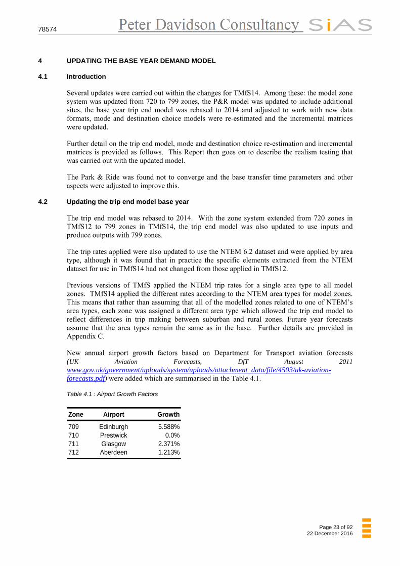
New annual airport growth factors based on Department for Transport aviation forecasts (UK Aviation Forecasts, DfT August 2011 www.gov.uk/government/uploads/system/uploads/attachment_data/file/4503/uk-aviation-forecasts.pdf) were added which are summarised in the Table 4.1.
Table 4.1 : Airport Growth Factors
Zone Airport Growth
709 Edinburgh 5.588%710 Prestwick 0.0%711 Glasgow 2.371%712 Aberdeen 1.213%

78574
Page 24 of 92 22 December 2016
The trip end model used data derived from the base and future year land use model outputs to factor up the base year trip ends. A set of base year trip ends split by purpose and time period was produced from the 2014 observed matrices. The trip ends needed to be split by household car availability, which was not available in the observed matrices, so the household car availability split in the TMfS12 base year trip ends was applied to the 2014 trip ends.
The trip end model was updated with additional changes to handle the change in the format of the demographic input files from TELMOS, to take account of the increased number of zones and to aggregate over income bands. While the TMfS14 demand model is not currently disaggregated by income band this update could facilitate any future demand model update of this nature.
The 2014 land use data was then used in both the base and scenario inputs for the base year trip end model run as an initial test. The resulting output trip ends were identical to the inputs. Additional checks were then carried out using TELMOS data for a 2037 forecast year, confirming that the trip end model was working correctly.

78574
Page 25 of 92 22 December 2016
5 ESTIMATION OF NEW MODE AND DESTINATION CHOICE COEFFICIENTS
5.1 Scope of update
The remit of the update was to re-estimate and update the coefficients rather than changing the model structure, which effectively has mode choice above destination choice in the hierarchy of responses.
It is, however, worth noting at this point that the estimations carried out appeared generally to support the view that destination choice is more sensitive than mode choice and should, thus, be beneath mode choice in the hierarchy. They therefore support the existing model structure and is consistent with WebTAG.
5.2 Methodology
Using the revealed preference information contained in the base year validated Road and PT trip matrices and network skims, the Visual Choice software package allowed the estimation of various model coefficients via discrete choice methodology.
There were various approaches available for estimation, and a number of constraints which needed to be taken into account. For example, use of a multinomial logit structure in the estimations would have been computationally quicker and easier than estimating a nested logit, but would not have produced scaling coefficients to apply to the mode choice. For the TMfS14 estimations a nested logit structure was used (with destination choice under mode choice) in order to obtain scaling coefficients, cost, log-cost, and intra-zonal coefficients. Nested choice models can be estimated by estimating each nest individually as multinomial logit, calculating the logsums and passing them up to the next level up in the hierarchy, however, it is much better , more robust, more rigorous, more theoretically sound and can give different answers if both nest levels are estimated simultaneously. We estimated both nest levels simultaneously, which is more difficult with unknown convergence and run times.
TMfS incorporates distinct coefficients for different household types which have different car-ownership levels, however, the estimation dataset, being based on the observed matrices, was not split by car availability level so separate estimations for 1 car, 2 car households, etc. could not be carried out. Instead the data was grouped to an all car available level and the estimations had to be carried out at this aggregate level.
We calculated zonal ASCs by hand for all zones in an iterative process. Firstly coefficients were be estimated based on no Alternative-Specific Constants (ASCs fixed at zero), these were run through the Cube demand model, then a set of ASCs were calculated to ‘correct’ the modelled share across destinations and modes predicted by the model. These were then input as fixed ASCs to a new estimation and the process repeated until the estimations are satisfactorily stable or converged.
With the nested logit structure and large number of zones, estimation run times were found to be very long. In order to allow overnight runs we adopted a sampling approach, working with just one part of the dataset at a time. The estimations were initially run with external (i.e. outside of the estimation software) calculation of 9 ASCs, one for each sector, however, under this approach the estimation process was not converging and the number of ASCs had to be increased to 32 based on division of the zones across local authority boundaries.

78574
Page 26 of 92 22 December 2016
It was also found that the Park & Ride was not converging and so action was taken to try and address that problem and make the model converge (see Section 3.1). The Park & Ride non-convergence exacerbated the problems with run times, and with the non-convergence of the ASCs.
Each of these samples were still substantial sized datasets, and in combination with the sector-level ASCs allowed overnight estimations and 24hr turnarounds for a full iteration of estimation, running the demand model in Cube and calculating a new set of ASCs ready for the next estimation run. Iterations 2 and 3 of the 32 sector ASCs appeared to give the best overall set of ASCs, so iteration 3 was used.
5.3 Sample selection
Samples of the order of about 1,000 records were used, and a set of 10 estimations were made from 10 different sets of data for each trip purpose. The resulting coefficients were then averaged across the sampled subsets.
The samples were selected at random according to the following approach for each purpose:
1 The master set of all trip records for the purpose in question was created
2 The proportion of this dataset required to provide a sample of approximately 1,000 records was determined, i.e. 1 in every n records (e.g. 1 in 40 records)
3 Random starting point x within the first n records determined
4 Records x, x+n, x+2n, x+3n… selected to form the sample
5 The process was repeated to get all ten sets of trip records, ensuring that no record was used twice
78574
Page 27 of 92 22 December 2016
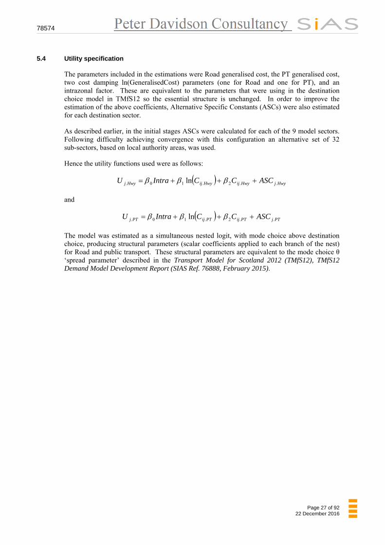
5.4 Utility specification
The parameters included in the estimations were Road generalised cost, the PT generalised cost, two cost damping ln(GeneralisedCost) parameters (one for Road and one for PT), and an intrazonal factor. These are equivalent to the parameters that were using in the destination choice model in TMfS12 so the essential structure is unchanged. In order to improve the estimation of the above coefficients, Alternative Specific Constants (ASCs) were also estimated for each destination sector.
As described earlier, in the initial stages ASCs were calculated for each of the 9 model sectors. Following difficulty achieving convergence with this configuration an alternative set of 32 sub-sectors, based on local authority areas, was used.
Hence the utility functions used were as follows:
HwyjHwyijHwyijHwyj ASCCCIntraU ..2.10. ln
and
PTjPTijPTijPTj ASCCCIntraU ..2.10. ln
The model was estimated as a simultaneous nested logit, with mode choice above destination choice, producing structural parameters (scalar coefficients applied to each branch of the nest) for Road and public transport. These structural parameters are equivalent to the mode choice θ ‘spread parameter’ described in the Transport Model for Scotland 2012 (TMfS12), TMfS12 Demand Model Development Report (SIAS Ref. 76888, February 2015).
78574
Page 28 of 92 22 December 2016
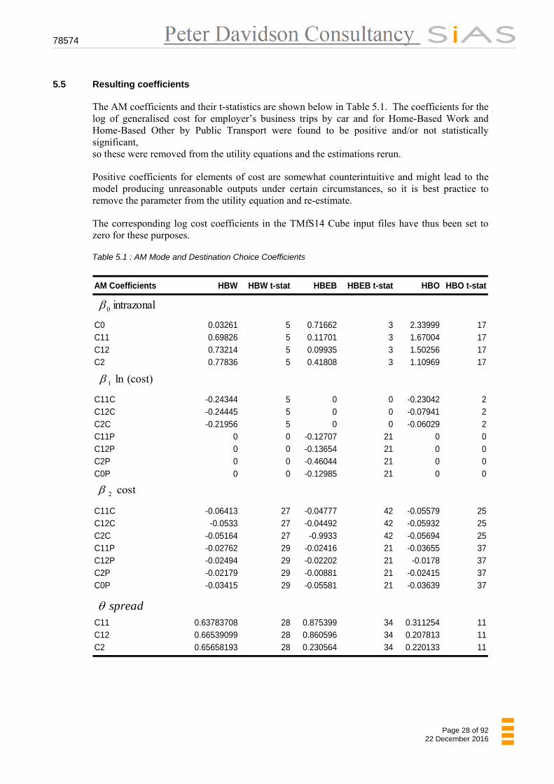
5.5 Resulting coefficients
The AM coefficients and their t-statistics are shown below in Table 5.1. The coefficients for the log of generalised cost for employer’s business trips by car and for Home-Based Work and Home-Based Other by Public Transport were found to be positive and/or not statistically significant, so these were removed from the utility equations and the estimations rerun.
Positive coefficients for elements of cost are somewhat counterintuitive and might lead to the model producing unreasonable outputs under certain circumstances, so it is best practice to remove the parameter from the utility equation and re-estimate.
The corresponding log cost coefficients in the TMfS14 Cube input files have thus been set to zero for these purposes.
Table 5.1 : AM Mode and Destination Choice Coefficients
AM Coefficients HBW HBW t-stat HBEB HBEB t-stat HBO HBO t-stat
C0 0.03261 5 0.71662 3 2.33999 17C11 0.69826 5 0.11701 3 1.67004 17C12 0.73214 5 0.09935 3 1.50256 17C2 0.77836 5 0.41808 3 1.10969 17
C11C -0.24344 5 0 0 -0.23042 2C12C -0.24445 5 0 0 -0.07941 2C2C -0.21956 5 0 0 -0.06029 2C11P 0 0 -0.12707 21 0 0C12P 0 0 -0.13654 21 0 0C2P 0 0 -0.46044 21 0 0C0P 0 0 -0.12985 21 0 0
C11C -0.06413 27 -0.04777 42 -0.05579 25C12C -0.0533 27 -0.04492 42 -0.05932 25C2C -0.05164 27 -0.9933 42 -0.05694 25C11P -0.02762 29 -0.02416 21 -0.03655 37C12P -0.02494 29 -0.02202 21 -0.0178 37C2P -0.02179 29 -0.00881 21 -0.02415 37C0P -0.03415 29 -0.05581 21 -0.03639 37
C11 0.63783708 28 0.875399 34 0.311254 11C12 0.66539099 28 0.860596 34 0.207813 11C2 0.65658193 28 0.230564 34 0.220133 11
intrazonal0
(cost)ln1
cost2
spread
78574
Page 29 of 92 22 December 2016
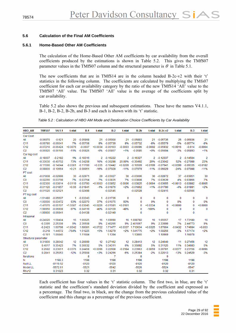
5.6 Calculation of the Final AM Coefficients
5.6.1 Home-Based Other AM Coefficients
The calculation of the Home-Based Other AM coefficients by car availability from the overall coefficients produced by the estimations is shown in Table 5.2. This gives the TMfS07 parameter values in the TMfS07 column and the structural parameter is in Table 5.1.
The new coefficients that are in TMfS14 are in the column headed B-2c-v2 with their ‘t’ statistics in the following column. The coefficients are calculated by multiplying the TMfs07 coefficient for each car availability category by the ratio of the new TMfS14 ‘All’ value to the TMfS07 ‘All’ value. The TMfS07 ‘All’ value is the average of the coefficients split by car availability.
Table 5.2 also shows the previous and subsequent estimations. These have the names V4.1.1, B-1, B-2, B-2, B-2b, and B-3 and each is shown with its ‘t’ statistic.
Table 5.2 : Calculation of HBO AM Mode and Destination Choice Coefficients by Car Availability
Each coefficient has four values in the ‘t’ statistic column. The first two, in blue, are the ‘t’ statistic and the coefficient’s standard deviation divided by the coefficient and expressed as a percentage. The final two, in black, are the change from the previous calculated value of the coefficient and this change as a percentage of the previous coefficient.
78574
Page 30 of 92 22 December 2016
The ‘t’ statistic for each coefficient is the value in the final cell on the ‘All’ row and is expressed below this as a percentage. The value below this is the difference between the coefficient and the value obtained on the previous estimation run, again expressed in the cell below it as a percentage.
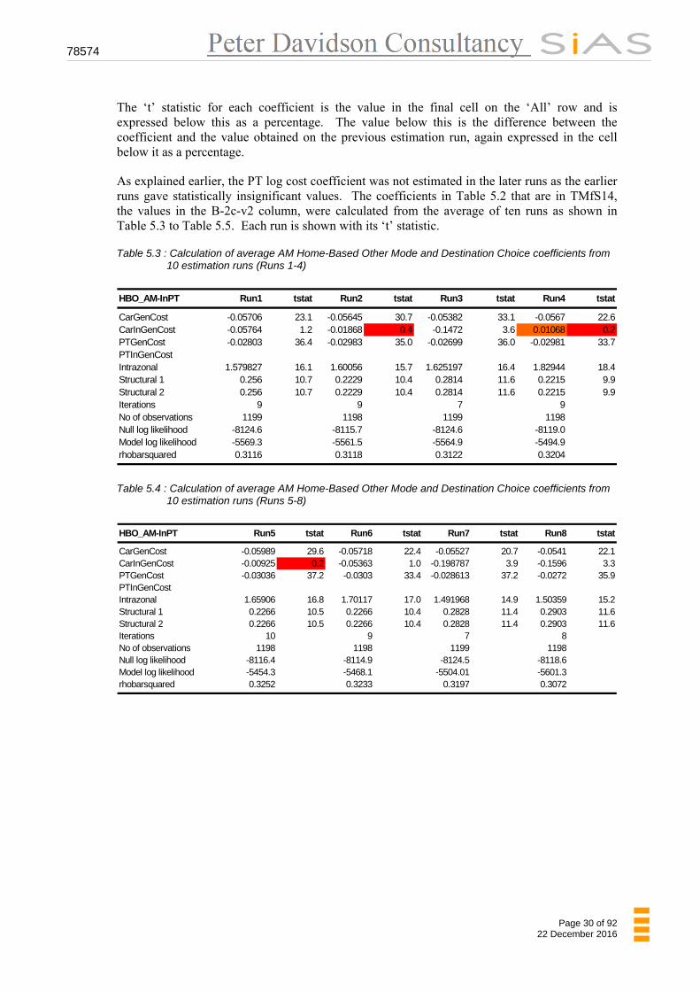
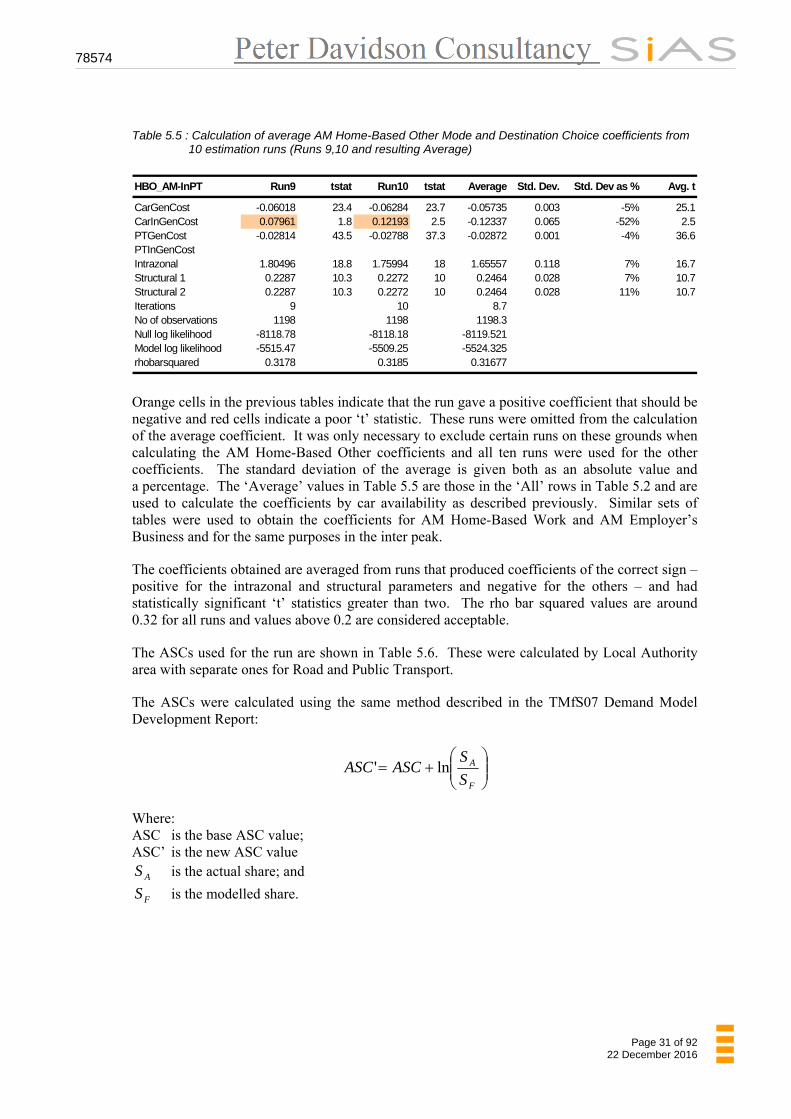
As explained earlier, the PT log cost coefficient was not estimated in the later runs as the earlier runs gave statistically insignificant values. The coefficients in Table 5.2 that are in TMfS14, the values in the B-2c-v2 column, were calculated from the average of ten runs as shown in Table 5.3 to Table 5.5. Each run is shown with its ‘t’ statistic.
Table 5.3 : Calculation of average AM Home-Based Other Mode and Destination Choice coefficients from
10 estimation runs (Runs 1-4)
HBO_AM-InPT Run1 tstat Run2 tstat Run3 tstat Run4 tstat
CarGenCost -0.05706 23.1 -0.05645 30.7 -0.05382 33.1 -0.0567 22.6CarInGenCost -0.05764 1.2 -0.01868 0.4 -0.1472 3.6 0.01068 0.2PTGenCost -0.02803 36.4 -0.02983 35.0 -0.02699 36.0 -0.02981 33.7PTInGenCostIntrazonal 1.579827 16.1 1.60056 15.7 1.625197 16.4 1.82944 18.4Structural 1 0.256 10.7 0.2229 10.4 0.2814 11.6 0.2215 9.9Structural 2 0.256 10.7 0.2229 10.4 0.2814 11.6 0.2215 9.9Iterations 9 9 7 9No of observations 1199 1198 1199 1198Null log likelihood -8124.6 -8115.7 -8124.6 -8119.0Model log likelihood -5569.3 -5561.5 -5564.9 -5494.9rhobarsquared 0.3116 0.3118 0.3122 0.3204
Table 5.4 : Calculation of average AM Home-Based Other Mode and Destination Choice coefficients from
10 estimation runs (Runs 5-8)
HBO_AM-InPT Run5 tstat Run6 tstat Run7 tstat Run8 tstat
CarGenCost -0.05989 29.6 -0.05718 22.4 -0.05527 20.7 -0.0541 22.1CarInGenCost -0.00925 0.2 -0.05363 1.0 -0.198787 3.9 -0.1596 3.3PTGenCost -0.03036 37.2 -0.0303 33.4 -0.028613 37.2 -0.0272 35.9PTInGenCostIntrazonal 1.65906 16.8 1.70117 17.0 1.491968 14.9 1.50359 15.2Structural 1 0.2266 10.5 0.2266 10.4 0.2828 11.4 0.2903 11.6Structural 2 0.2266 10.5 0.2266 10.4 0.2828 11.4 0.2903 11.6Iterations 10 9 7 8No of observations 1198 1198 1199 1198Null log likelihood -8116.4 -8114.9 -8124.5 -8118.6Model log likelihood -5454.3 -5468.1 -5504.01 -5601.3rhobarsquared 0.3252 0.3233 0.3197 0.3072
78574
Page 31 of 92 22 December 2016
Table 5.5 : Calculation of average AM Home-Based Other Mode and Destination Choice coefficients from
10 estimation runs (Runs 9,10 and resulting Average)
HBO_AM-InPT Run9 tstat Run10 tstat Average Std. Dev. Std. Dev as % Avg. t
CarGenCost -0.06018 23.4 -0.06284 23.7 -0.05735 0.003 -5% 25.1CarInGenCost 0.07961 1.8 0.12193 2.5 -0.12337 0.065 -52% 2.5PTGenCost -0.02814 43.5 -0.02788 37.3 -0.02872 0.001 -4% 36.6PTInGenCostIntrazonal 1.80496 18.8 1.75994 18 1.65557 0.118 7% 16.7Structural 1 0.2287 10.3 0.2272 10 0.2464 0.028 7% 10.7Structural 2 0.2287 10.3 0.2272 10 0.2464 0.028 11% 10.7Iterations 9 10 8.7No of observations 1198 1198 1198.3Null log likelihood -8118.78 -8118.18 -8119.521Model log likelihood -5515.47 -5509.25 -5524.325rhobarsquared 0.3178 0.3185 0.31677
Orange cells in the previous tables indicate that the run gave a positive coefficient that should be negative and red cells indicate a poor ‘t’ statistic. These runs were omitted from the calculation of the average coefficient. It was only necessary to exclude certain runs on these grounds when calculating the AM Home-Based Other coefficients and all ten runs were used for the other coefficients. The standard deviation of the average is given both as an absolute value and a percentage. The ‘Average’ values in Table 5.5 are those in the ‘All’ rows in Table 5.2 and are used to calculate the coefficients by car availability as described previously. Similar sets of tables were used to obtain the coefficients for AM Home-Based Work and AM Employer’s Business and for the same purposes in the inter peak.
The coefficients obtained are averaged from runs that produced coefficients of the correct sign – positive for the intrazonal and structural parameters and negative for the others – and had statistically significant ‘t’ statistics greater than two. The rho bar squared values are around 0.32 for all runs and values above 0.2 are considered acceptable.
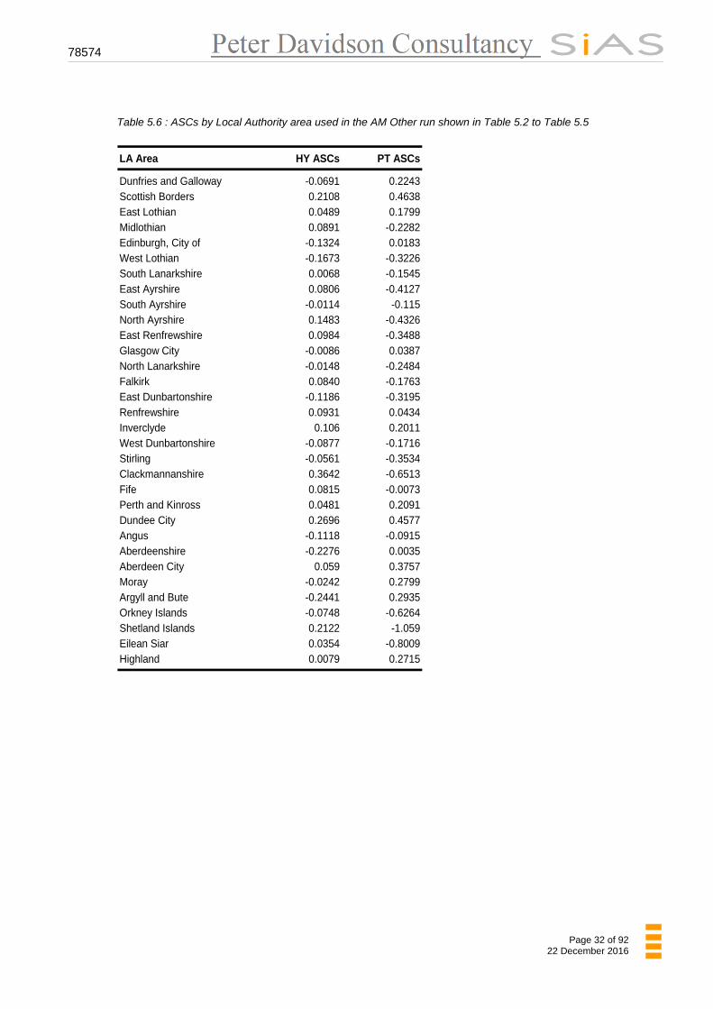
The ASCs used for the run are shown in Table 5.6. These were calculated by Local Authority area with separate ones for Road and Public Transport.
The ASCs were calculated using the same method described in the TMfS07 Demand Model Development Report:
F
A
S
SASCASC ln'
Where: ASC is the base ASC value; ASC’ is the new ASC value
AS is the actual share; and
FS is the modelled share.
78574
Page 32 of 92 22 December 2016
Table 5.6 : ASCs by Local Authority area used in the AM Other run shown in Table 5.2 to Table 5.5
LA Area HY ASCs PT ASCs
Dunfries and Galloway -0.0691 0.2243Scottish Borders 0.2108 0.4638East Lothian 0.0489 0.1799Midlothian 0.0891 -0.2282Edinburgh, City of -0.1324 0.0183West Lothian -0.1673 -0.3226South Lanarkshire 0.0068 -0.1545East Ayrshire 0.0806 -0.4127South Ayrshire -0.0114 -0.115North Ayrshire 0.1483 -0.4326East Renfrewshire 0.0984 -0.3488Glasgow City -0.0086 0.0387North Lanarkshire -0.0148 -0.2484Falkirk 0.0840 -0.1763East Dunbartonshire -0.1186 -0.3195Renfrewshire 0.0931 0.0434Inverclyde 0.106 0.2011West Dunbartonshire -0.0877 -0.1716Stirling -0.0561 -0.3534Clackmannanshire 0.3642 -0.6513Fife 0.0815 -0.0073Perth and Kinross 0.0481 0.2091Dundee City 0.2696 0.4577Angus -0.1118 -0.0915Aberdeenshire -0.2276 0.0035Aberdeen City 0.059 0.3757Moray -0.0242 0.2799Argyll and Bute -0.2441 0.2935Orkney Islands -0.0748 -0.6264Shetland Islands 0.2122 -1.059Eilean Siar 0.0354 -0.8009Highland 0.0079 0.2715
78574
Page 33 of 92 22 December 2016
5.6.2 Home-Based Work AM Coefficients
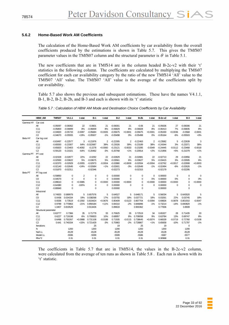
The calculation of the Home-Based Work AM coefficients by car availability from the overall coefficients produced by the estimations is shown in Table 5.7. This gives the TMfS07 parameter values in the TMfS07 column and the structural parameter is in Table 5.1.
The new coefficients that are in TMfS14 are in the column headed B-2c-v2 with their ‘t’ statistics in the following column. The coefficients are calculated by multiplying the TMfs07 coefficient for each car availability category by the ratio of the new TMfS14 ‘All’ value to the TMfS07 ‘All’ value. The TMfS07 ‘All’ value is the average of the coefficients split by car availability.
Table 5.7 also shows the previous and subsequent estimations. These have the names V4.1.1, B-1, B-2, B-2, B-2b, and B-3 and each is shown with its ‘t’ statistic
Table 5.7 : Calculation of HBW AM Mode and Destination Choice Coefficients by Car Availability
HBW_AM TMfS07 V4.1.1 t-stat B-1 t-stat B-2 t-stat B-2b t-stat B-2c-v2 t-stat B-3 t-stat
Gamma HY Car costAll -0.05097 -0.06062 22 -0.0601 21 -0.06001 21 -0.06 21 -0.05636 27 -0.06006 21C11 -0.05800 -0.06899 8% -0.06839 8% -0.06829 8% -0.06828 8% -0.06413 7% -0.06835 8%C12 -0.04820 -0.05733 -0.0097 -0.05684 +0.0005 -0.05675 +0.0001 -0.05675 +0.0001 -0.05330 +0.0036 -0.0568 -0.0001C2 -0.04670 -0.05555 +19% -0.05507 -1% -0.05498 0% -0.05498 0% -0.05164 -6% -0.05503 +0%
Beta HY Car log costAll -0.63497 -0.22577 3 -0.21976 2 -0.22305 2 -0.22463 2 -0.23582 5 -0.22639 3C11 -0.65550 -0.23307 64% -0.022687 39% -0.23026 39% -0.23189 38% -0.24344 3% -0.23371 38%C12 -0.65820 -0.23403 +0.4092 -0.2278 +0.0060 -0.23121 -0.0033 -0.23285 -0.0049 -0.24445 -0.0112 -0.23468 -0.0018C2 -0.59120 -0.21021 -64% -0.20462 -3% -0.20768 +1% -0.20914 +2% -0.21956 +5% -0.21079 +1%
Gamma PT PT costAll -0.02328 -0.02877 22% -0.0292 22 -0.02829 21 -0.02881 22 -0.02713 29 -0.02856 21C0 -0.02930 -0.03622 5% -0.03675 5% -0.03561 6% -0.03627 5% -0.03415 3% -0.03595 6%C11 -0.02370 -0.02929 -0.0055 -0.02973 -0.0004 -0.02880 +0.0009 -0.02934 +0.0004 -0.02762 +0.0017 -0.02908 +0.0003C12 -0.02140 -0.02645 +24% -0.02684 +1% -0.02601 -3% -0.02649 -1% -0.02494 -6% -0.02626 -1%C2 -0.01870 -0.02311 -0.02346 -0.02273 -0.02315 -0.02179 -0.02295
Beta PT PT log costAll -0.59850 0 2 0 0 0.00000 0 0 0 0.00000 0 0 0C0 -0.04570 0 0 0 0 0.00000 0 0 0% 0.00000 0% 0 0%C11 -0.89610 0 +0.5985 0 +0.0000 0.00000 +0.0000 0 +0.0000 0.00000 +0.0000 0 +0.0000C12 -0.64380 0 -100% 0 0 0.00000 0 0 0 0.00000 0 0 0C2 -0.80840 0 0 0.00000 0 0.00000 0IntrazonalAll 0.74920 0.589979 5 0.657576 5 0.64527 5 0.648171 5 0.56034 5 0.643520 5C0 0.0436 0.034334 19% 0.038268 17% 0.03755 18% 0.037721 18% 0.03261 22% 0.03745 18%C11 0.9336 0.73519 -0.1592 0.819424 +0.0676 0.80409 -0.0123 0.807704 -0.0094 0.69826 -0.0878 0.801910 -0.0047C12 0.9789 0.770863 -21% 0.859184 +11% 0.84310 -2% 0.846896 -1% 0.73214 -14% 0.840820 -1%C2 1.0407 0.819529 0.913426 0.89633 0.900362 0.77836 0.8939Structural parameterAll 0.63777 0.7366 35 0.71779 33 0.70625 26 0.72519 34 0.65327 28 0.71435 33C11 0.6227 0.719198 6% 0.700833 10% 0.68957 8% 0.708058 9% 0.63784 13% 0.69747 8%C12 0.6496 0.750267 +0.0988 0.731108 -0.0188 0.71935 -0.0115 0.738645 +0.0074 0.66539 -0.0719 0.72760 -0.0108C2 0.641 0.740334 +15% 0.721429 -3% 0.70983 -2% 0.728867 +1% 0.65658 -10% 0.71797 -1%Iterations 25 19 25 19 0N 1200 1200 1200 1200 1200 1200Null LL -8128 -8128 -8128 -8128 -8128 -8128Model LL -5596 -5599 -5599 -5586 -5587 -5577Rho^2 0.31 0.31 0.31 0.31 0.30968 0.31
The coefficients in Table 5.7 that are in TMfS14, the values in the B-2c-v2 column, were calculated from the average of ten runs as shown in Table 5.8 . Each run is shown with its ‘t’ statistic.
78574
Page 34 of 92 22 December 2016
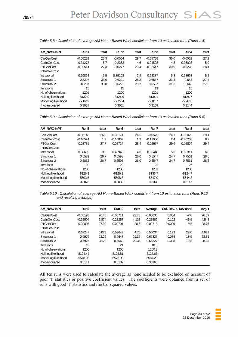
Table 5.8 : Calculation of average AM Home-Based Work coefficient from 10 estimation runs (Runs 1-4)
AM_NWC-InPT Run1 tstat Run2 tstat Run3 tstat Run4 tstat
CarGenCost -0.05282 23.3 -0.0564 29.7 -0.05758 35.0 -0.0562 27.2CarInGenCost -0.31272 5.7 -0.2363 4.6 -0.21593 4.8 -0.26008 5.0PTGenCost -0.02514 27.3 -0.0277 29.4 -0.02647 30.9 -0.0278 28.4PTInGenCostIntrazonal 0.69864 6.5 0.35103 2.9 0.58387 5.3 0.58693 5.2Structural 1 0.8207 33.0 0.6221 28.2 0.6557 31.3 0.643 27.6Structural 2 0.8207 33.0 0.6221 28.2 0.6557 31.3 0.643 27.6Iterations 15 15 19 15No of observations 1201 1200 1201 1200Null log likelihood -8132.0 -8124.9 -8134.1 -8124.7Model log likelihood -5602.9 -5622.4 -5581.7 -5547.3rhobarsquared 0.3081 0.3051 0.3109 0.3144
Table 5.9 : Calculation of average AM Home-Based Work coefficient from 10 estimation runs (Runs 5-8)
AM_NWC-InPT Run5 tstat Run6 tstat Run7 tstat Run8 tstat
CarGenCost -0.06148 26.0 -0.06174 24.6 -0.0575 24.7 -0.05079 29.1CarInGenCost -0.10524 1.9 -0.10867 1.9 -0.12906 2.4 -0.40258 8.2PTGenCost -0.02735 27.7 -0.02714 28.4 -0.02657 29.6 -0.02804 29.4PTInGenCostIntrazonal 0.38693 3.2 0.46948 4.0 0.66448 5.8 0.65311 6.0Structural 1 0.5582 26.7 0.5598 26.0 0.5547 24.7 0.7561 28.5Structural 2 0.5882 26.7 0.5598 26.0 0.5547 24.7 0.7561 28.5Iterations 20 22 22 26No of observations 1200 1200 1201 1200Null log likelihood 8126.3 -8126.1 8133.7 -8124.7Model log likelihood -5603.5 -5598.3 -5647.0 -5544.3rhobarsquared 0.3076 0.3082 0.3028 0.3147
Table 5.10 : Calculation of average AM Home-Based Work coefficient from 10 estimation runs (Runs 9,10
and resulting average)
AM_NWC-InPT Run9 tstat Run10 tstat Average Std. Dev.d. Dev as % Avg. t
CarGenCost -0.05193 26.43 -0.05711 22.78 -0.05636 0.004 -7% 26.89CarInGenCost -0.35504 6.874 -0.23257 4.133 -0.23582 0.102 -43% 4.548PTGenCost -0.02803 27.92 -0.02701 28.6 -0.02713 0.0009 -3% 28.76PTInGenCostIntrazonal 0.67247 6.079 0.53649 4.75 0.56034 0.123 22% 4.989Structural 1 0.6976 28.22 0.6648 29.35 0.65327 0.088 13% 28.35Structural 2 0.6976 28.22 0.6648 29.35 0.65327 0.088 13% 28.35Iterations 13 21 18.8No of observations 1200 1200 1200.3Null log likelihood -8124.44 -8125.81 -8127.68Model log likelihood -5548.93 -5575.93 -5587.23rhobarsquared 0.3141 0.3109 0.30968
All ten runs were used to calculate the average as none needed to be excluded on account of poor ‘t’ statistics or positive coefficient values. The coefficients were obtained from a set of runs with good ‘t’ statistics and rho bar squared values.
78574
Page 35 of 92 22 December 2016
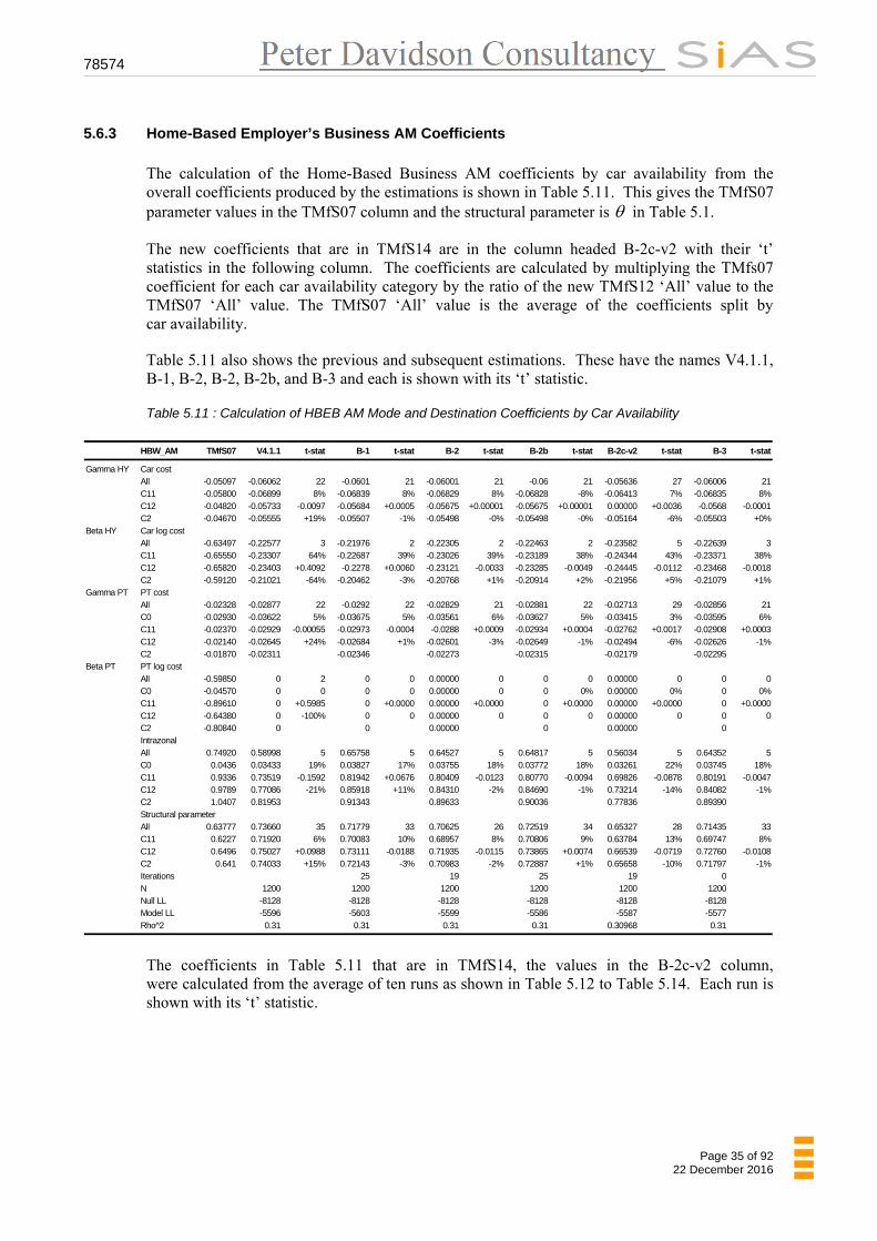
5.6.3 Home-Based Employer’s Business AM Coefficients
The calculation of the Home-Based Business AM coefficients by car availability from the overall coefficients produced by the estimations is shown in Table 5.11. This gives the TMfS07 parameter values in the TMfS07 column and the structural parameter is in Table 5.1.
The new coefficients that are in TMfS14 are in the column headed B-2c-v2 with their ‘t’ statistics in the following column. The coefficients are calculated by multiplying the TMfs07 coefficient for each car availability category by the ratio of the new TMfS12 ‘All’ value to the TMfS07 ‘All’ value. The TMfS07 ‘All’ value is the average of the coefficients split by car availability.
Table 5.11 also shows the previous and subsequent estimations. These have the names V4.1.1, B-1, B-2, B-2, B-2b, and B-3 and each is shown with its ‘t’ statistic.
Table 5.11 : Calculation of HBEB AM Mode and Destination Coefficients by Car Availability
HBW_AM TMfS07 V4.1.1 t-stat B-1 t-stat B-2 t-stat B-2b t-stat B-2c-v2 t-stat B-3 t-stat
Gamma HY Car costAll -0.05097 -0.06062 22 -0.0601 21 -0.06001 21 -0.06 21 -0.05636 27 -0.06006 21C11 -0.05800 -0.06899 8% -0.06839 8% -0.06829 8% -0.06828 -8% -0.06413 7% -0.06835 8%C12 -0.04820 -0.05733 -0.0097 -0.05684 +0.0005 -0.05675 +0.00001 -0.05675 +0.00001 0.00000 +0.0036 -0.0568 -0.0001C2 -0.04670 -0.05555 +19% -0.05507 -1% -0.05498 -0% -0.05498 -0% -0.05164 -6% -0.05503 +0%
Beta HY Car log costAll -0.63497 -0.22577 3 -0.21976 2 -0.22305 2 -0.22463 2 -0.23582 5 -0.22639 3C11 -0.65550 -0.23307 64% -0.22687 39% -0.23026 39% -0.23189 38% -0.24344 43% -0.23371 38%C12 -0.65820 -0.23403 +0.4092 -0.2278 +0.0060 -0.23121 -0.0033 -0.23285 -0.0049 -0.24445 -0.0112 -0.23468 -0.0018C2 -0.59120 -0.21021 -64% -0.20462 -3% -0.20768 +1% -0.20914 +2% -0.21956 +5% -0.21079 +1%
Gamma PT PT costAll -0.02328 -0.02877 22 -0.0292 22 -0.02829 21 -0.02881 22 -0.02713 29 -0.02856 21C0 -0.02930 -0.03622 5% -0.03675 5% -0.03561 6% -0.03627 5% -0.03415 3% -0.03595 6%C11 -0.02370 -0.02929 -0.00055 -0.02973 -0.0004 -0.0288 +0.0009 -0.02934 +0.0004 -0.02762 +0.0017 -0.02908 +0.0003C12 -0.02140 -0.02645 +24% -0.02684 +1% -0.02601 -3% -0.02649 -1% -0.02494 -6% -0.02626 -1%C2 -0.01870 -0.02311 -0.02346 -0.02273 -0.02315 -0.02179 -0.02295
Beta PT PT log costAll -0.59850 0 2 0 0 0.00000 0 0 0 0.00000 0 0 0C0 -0.04570 0 0 0 0 0.00000 0 0 0% 0.00000 0% 0 0%C11 -0.89610 0 +0.5985 0 +0.0000 0.00000 +0.0000 0 +0.0000 0.00000 +0.0000 0 +0.0000C12 -0.64380 0 -100% 0 0 0.00000 0 0 0 0.00000 0 0 0C2 -0.80840 0 0 0.00000 0 0.00000 0IntrazonalAll 0.74920 0.58998 5 0.65758 5 0.64527 5 0.64817 5 0.56034 5 0.64352 5C0 0.0436 0.03433 19% 0.03827 17% 0.03755 18% 0.03772 18% 0.03261 22% 0.03745 18%C11 0.9336 0.73519 -0.1592 0.81942 +0.0676 0.80409 -0.0123 0.80770 -0.0094 0.69826 -0.0878 0.80191 -0.0047C12 0.9789 0.77086 -21% 0.85918 +11% 0.84310 -2% 0.84690 -1% 0.73214 -14% 0.84082 -1%C2 1.0407 0.81953 0.91343 0.89633 0.90036 0.77836 0.89390Structural parameterAll 0.63777 0.73660 35 0.71779 33 0.70625 26 0.72519 34 0.65327 28 0.71435 33C11 0.6227 0.71920 6% 0.70083 10% 0.68957 8% 0.70806 9% 0.63784 13% 0.69747 8%C12 0.6496 0.75027 +0.0988 0.73111 -0.0188 0.71935 -0.0115 0.73865 +0.0074 0.66539 -0.0719 0.72760 -0.0108C2 0.641 0.74033 +15% 0.72143 -3% 0.70983 -2% 0.72887 +1% 0.65658 -10% 0.71797 -1%Iterations 25 19 25 19 0N 1200 1200 1200 1200 1200 1200Null LL -8128 -8128 -8128 -8128 -8128 -8128Model LL -5596 -5603 -5599 -5586 -5587 -5577Rho^2 0.31 0.31 0.31 0.31 0.30968 0.31
The coefficients in Table 5.11 that are in TMfS14, the values in the B-2c-v2 column, were calculated from the average of ten runs as shown in Table 5.12 to Table 5.14. Each run is shown with its ‘t’ statistic.
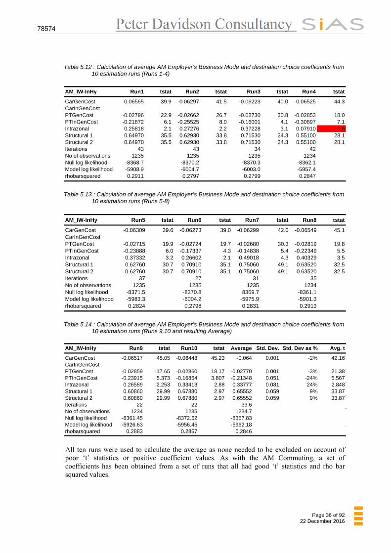
78574
Page 36 of 92 22 December 2016
Table 5.12 : Calculation of average AM Employer’s Business Mode and destination choice coefficients from
10 estimation runs (Runs 1-4)
AM_IW-InHy Run1 tstat Run2 tstat Run3 tstat Run4 tstat
CarGenCost -0.06565 39.9 -0.06297 41.5 -0.06223 40.0 -0.06525 44.3CarInGenCostPTGenCost -0.02796 22.9 -0.02662 26.7 -0.02730 20.8 -0.02853 18.0PTInGenCost -0.21872 6.1 -0.25525 8.0 -0.16001 4.1 -0.30897 7.1Intrazonal 0.25818 2.1 0.27276 2.2 0.37228 3.1 0.07910 0.6Structural 1 0.64970 35.5 0.62930 33.8 0.71530 34.3 0.55100 28.1Structural 2 0.64970 35.5 0.62930 33.8 0.71530 34.3 0.55100 28.1Iterations 43 43 34 42No of observations 1235 1235 1235 1234Null log likelihood -8368.7 -8370.2 -8370.3 -8362.1Model log likelihood -5908.9 -6004.7 -6003.0 -5957.4rhobarsquared 0.2911 0.2797 0.2799 0.2847
Table 5.13 : Calculation of average AM Employer’s Business Mode and destination choice coefficients from
10 estimation runs (Runs 5-8)
AM_IW-InHy Run5 tstat Run6 tstat Run7 tstat Run8 tstat
CarGenCost -0.06309 39.6 -0.06273 39.0 -0.06299 42.0 -0.06549 45.1CarInGenCostPTGenCost -0.02715 19.9 -0.02724 19.7 -0.02680 30.3 -0.02819 19.8PTInGenCost -0.23888 6.0 -0.17337 4.3 -0.14838 5.4 -0.22349 5.5Intrazonal 0.37332 3.2 0.26602 2.1 0.49018 4.3 0.40329 3.5Structural 1 0.62760 30.7 0.70910 35.1 0.75060 49.1 0.63520 32.5Structural 2 0.62760 30.7 0.70910 35.1 0.75060 49.1 0.63520 32.5Iterations 37 27 31 35No of observations 1235 1235 1235 1234Null log likelihood -8371.5 -8370.8 8369.7 -8361.1Model log likelihood -5983.3 -6004.2 -5975.9 -5901.3rhobarsquared 0.2824 0.2798 0.2831 0.2913
Table 5.14 : Calculation of average AM Employer’s Business Mode and destination choice coefficients from 10 estimation runs (Runs 9,10 and resulting Average)
AM_IW-InHy Run9 tstat Run10 tstat Average Std. Dev. Std. Dev as % Avg. t
CarGenCost -0.06517 45.05 -0.06448 45.23 -0.064 0.001 -2% 42.16CarInGenCostPTGenCost -0.02859 17.65 -0.02860 18.17 -0.02770 0.001 -3% 21.38PTInGenCost -0.23915 5.373 -0.16854 3.807 -0.21348 0.051 -24% 5.567Intrazonal 0.26589 2.253 0.33413 2.88 0.33777 0.081 24% 2.848Structural 1 0.60860 29.99 0.67880 2.97 0.65552 0.059 9% 33.87Structural 2 0.60860 29.99 0.67880 2.97 0.65552 0.059 9% 33.87Iterations 22 22 33.6No of observations 1234 1235 1234.7Null log likelihood -8361.45 -8372.52 -8367.83Model log likelihood -5926.63 -5956.45 -5962.18rhobarsquared 0.2883 0.2857 0.2846
All ten runs were used to calculate the average as none needed to be excluded on account of poor ‘t’ statistics or positive coefficient values. As with the AM Commuting, a set of coefficients has been obtained from a set of runs that all had good ‘t’ statistics and rho bar squared values.
78574
Page 37 of 92 22 December 2016
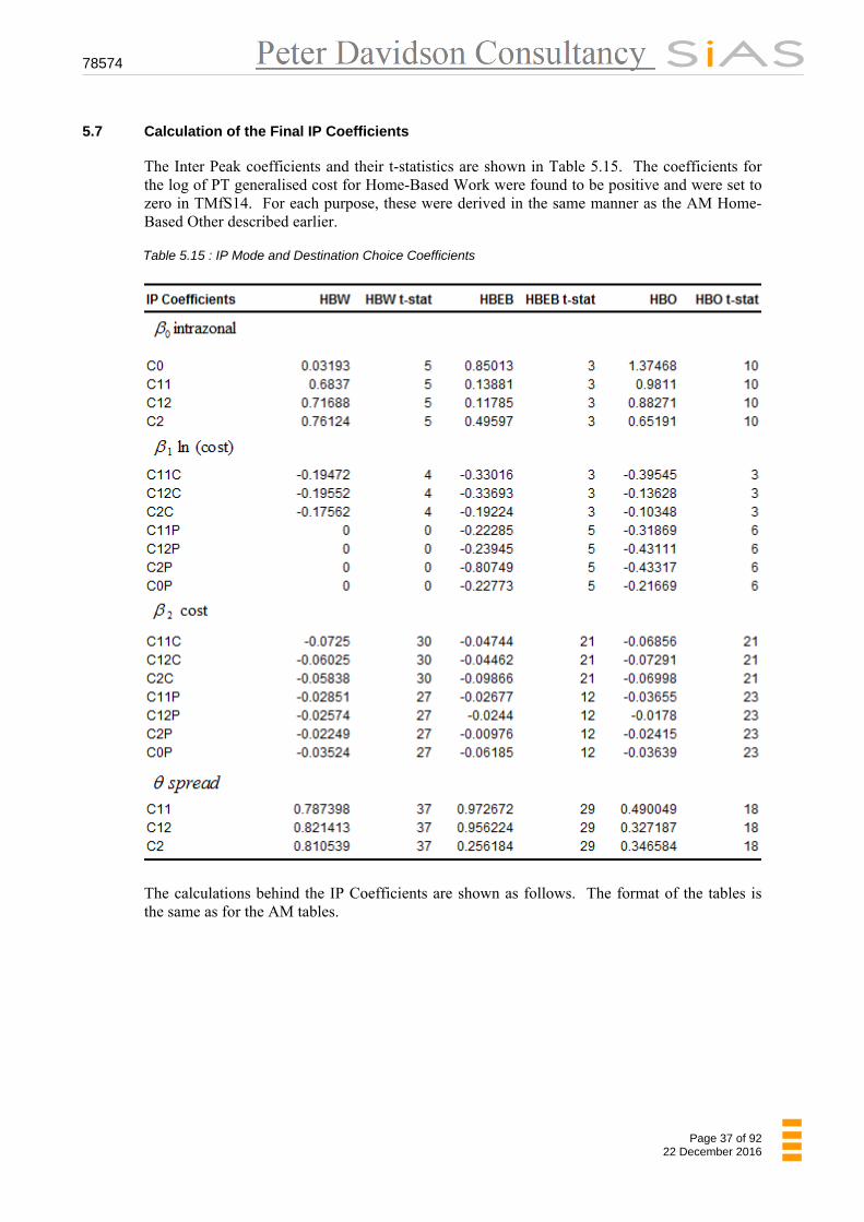
5.7 Calculation of the Final IP Coefficients
The Inter Peak coefficients and their t-statistics are shown in Table 5.15. The coefficients for the log of PT generalised cost for Home-Based Work were found to be positive and were set to zero in TMfS14. For each purpose, these were derived in the same manner as the AM Home-Based Other described earlier.
Table 5.15 : IP Mode and Destination Choice Coefficients
The calculations behind the IP Coefficients are shown as follows. The format of the tables is the same as for the AM tables.
78574
Page 38 of 92 22 December 2016
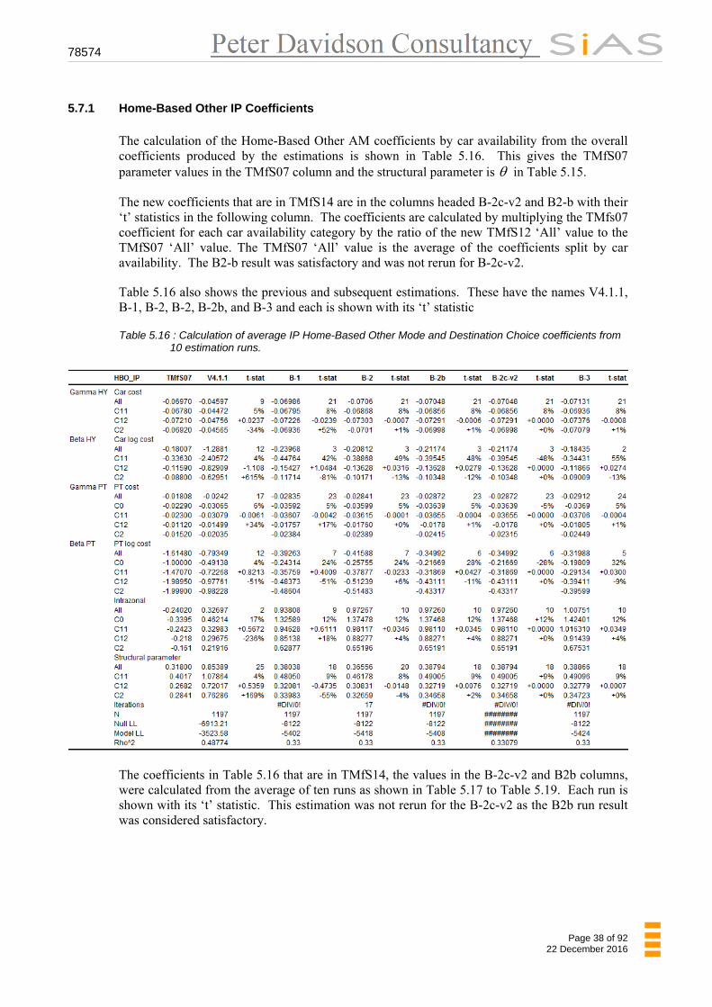
5.7.1 Home-Based Other IP Coefficients
The calculation of the Home-Based Other AM coefficients by car availability from the overall coefficients produced by the estimations is shown in Table 5.16. This gives the TMfS07 parameter values in the TMfS07 column and the structural parameter is in Table 5.15.
The new coefficients that are in TMfS14 are in the columns headed B-2c-v2 and B2-b with their ‘t’ statistics in the following column. The coefficients are calculated by multiplying the TMfs07 coefficient for each car availability category by the ratio of the new TMfS12 ‘All’ value to the TMfS07 ‘All’ value. The TMfS07 ‘All’ value is the average of the coefficients split by car availability. The B2-b result was satisfactory and was not rerun for B-2c-v2.
Table 5.16 also shows the previous and subsequent estimations. These have the names V4.1.1, B-1, B-2, B-2, B-2b, and B-3 and each is shown with its ‘t’ statistic
Table 5.16 : Calculation of average IP Home-Based Other Mode and Destination Choice coefficients from
10 estimation runs.
The coefficients in Table 5.16 that are in TMfS14, the values in the B-2c-v2 and B2b columns, were calculated from the average of ten runs as shown in Table 5.17 to Table 5.19. Each run is shown with its ‘t’ statistic. This estimation was not rerun for the B-2c-v2 as the B2b run result was considered satisfactory.
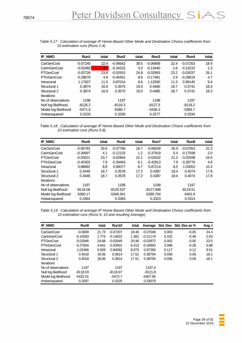
78574
Page 39 of 92 22 December 2016
Table 5.17 : Calculation of average IP Home-Based Other Mode and Destination Choice coefficients from
10 estimation runs (Runs 1-4)
IP_NWO Run1 tstat Run2 tstat Run3 tstat Run4 tstat
CarGenCost -0.07245 22.4 -0.06642 38.5 -0.06888 22.4 -0.07263 18.4CarInGenCost -0.02482 0.3 -0.34315 5.0 -0.13440 1.6 -0.13215 1.3PTGenCost -0.02726 23.6 -0.02915 24.8 -0.02993 23.2 -0.03037 26.1PTInGenCost -0.28676 4.8 -0.46451 8.6 -0.17481 2.9 -0.29619 4.7Intrazonal 1.17927 11.5 0.87014 8.6 1.12930 11.3 0.99145 9.4Structural 1 0.3874 16.9 0.3575 19.0 0.4485 18.7 0.3741 18.3Structural 2 0.3874 16.9 0.3575 19.0 0.4485 18.7 0.3741 18.3IterationsNo of observations 1198 1197 1198 1197Null log likelihood -8126.2 -8118.3 -8127.5 -8118.2Model log likelihood -5471.5 -5380.7 -5436.3 -5384.7rhobarsquared 0.3233 0.3339 0.3277 0.3334
Table 5.18 : Calculation of average IP Home-Based Other Mode and Destination Choice coefficients from 10 estimation runs (Runs 5-8)
IP_NWO Run5 tstat Run6 tstat Run7 tstat Run8 tstat
CarGenCost -0.06793 29.6 -0.07766 18.7 -0.06639 30.9 -0.07053 22.3CarInGenCost -0.30697 4.1 -0.12133 1.2 -0.37919 5.4 -0.17938 2.0PTGenCost -0.03021 23.7 -0.02864 22.1 -0.02632 21.2 -0.02938 24.4PTInGenCost -0.45303 7.9 -0.39463 6.1 -0.42913 7.9 -0.28776 4.8Intrazonal 0.88682 8.8 0.90077 8.7 0.87214 8.5 1.03052 10.3Structural 1 0.3448 18.7 0.3578 17.2 0.4387 18.4 0.4074 17.8Structural 2 0.3448 18.7 0.3578 17.2 0.4387 18.4 0.4074 17.8IterationsNo of observations 1197 1198 1198 1197Null log likelihood -8118.08 -8125.537 -8127.698 -8119.51Model log likelihood -5360.17 -5349.341 -5399.704 -5401.8rhobarsquared 0.3364 0.3383 0.3323 0.3314
Table 5.19 : Calculation of average IP Home-Based Other Mode and Destination Choice coefficients from 10 estimation runs (Runs 9, 10 and resulting Average)
IP_NWO Run9 tstat Run10 tstat Average Std. Dev. Std. Dev as % Avg. t
CarGenCost -0.0699 21.73 -0.07207 18.46 -0.07048 0.003 -0.05 24.4CarInGenCost -0.16283 1.774 -0.14622 1.381 -0.21174 0.102 -0.48 2.63PTGenCost -0.02946 24.68 -0.02649 20.96 -0.02872 0.002 -0.05 23.5PTInGenCost -0.27834 4.641 -0.43401 6.413 -0.34992 0.098 -0.28 5.88Intrazonal 1.02466 9.928 0.84092 8.073 0.97260 0.117 0.12 9.51Structural 1 0.4018 18.06 0.3614 17.51 0.38794 0.036 0.09 18.1Structural 2 0.4018 18.06 0.3614 17.51 0.38794 0.036 0.09 18.1Iterations No of observations 1197 1197 1197.4 Null log likelihood -8118.03 -8118.97 -8121.8 Model log likelihood -5422.51 -5472.7 -5407.95 rhobarsquared 0.3287 0.3225 0.33079
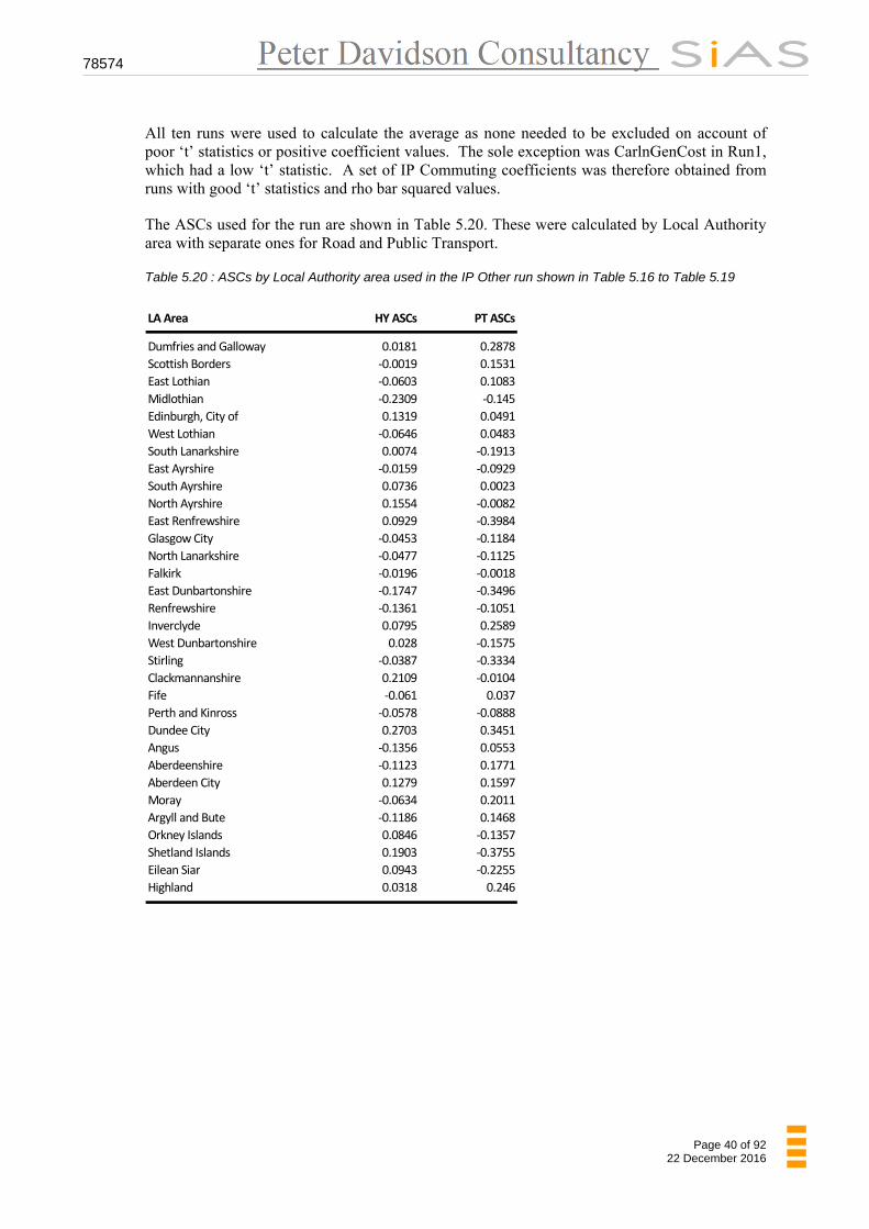
78574
Page 40 of 92 22 December 2016
All ten runs were used to calculate the average as none needed to be excluded on account of poor ‘t’ statistics or positive coefficient values. The sole exception was CarlnGenCost in Run1, which had a low ‘t’ statistic. A set of IP Commuting coefficients was therefore obtained from runs with good ‘t’ statistics and rho bar squared values.
The ASCs used for the run are shown in Table 5.20. These were calculated by Local Authority area with separate ones for Road and Public Transport.
Table 5.20 : ASCs by Local Authority area used in the IP Other run shown in Table 5.16 to Table 5.19
LA Area HY ASCs PT ASCs
Dumfries and Galloway 0.0181 0.2878
Scottish Borders -0.0019 0.1531
East Lothian -0.0603 0.1083
Midlothian -0.2309 -0.145
Edinburgh, City of 0.1319 0.0491
West Lothian -0.0646 0.0483
South Lanarkshire 0.0074 -0.1913
East Ayrshire -0.0159 -0.0929
South Ayrshire 0.0736 0.0023
North Ayrshire 0.1554 -0.0082
East Renfrewshire 0.0929 -0.3984
Glasgow City -0.0453 -0.1184
North Lanarkshire -0.0477 -0.1125
Falkirk -0.0196 -0.0018
East Dunbartonshire -0.1747 -0.3496
Renfrewshire -0.1361 -0.1051
Inverclyde 0.0795 0.2589
West Dunbartonshire 0.028 -0.1575
Stirling -0.0387 -0.3334
Clackmannanshire 0.2109 -0.0104
Fife -0.061 0.037
Perth and Kinross -0.0578 -0.0888
Dundee City 0.2703 0.3451
Angus -0.1356 0.0553
Aberdeenshire -0.1123 0.1771
Aberdeen City 0.1279 0.1597
Moray -0.0634 0.2011
Argyll and Bute -0.1186 0.1468
Orkney Islands 0.0846 -0.1357
Shetland Islands 0.1903 -0.3755
Eilean Siar 0.0943 -0.2255
Highland 0.0318 0.246
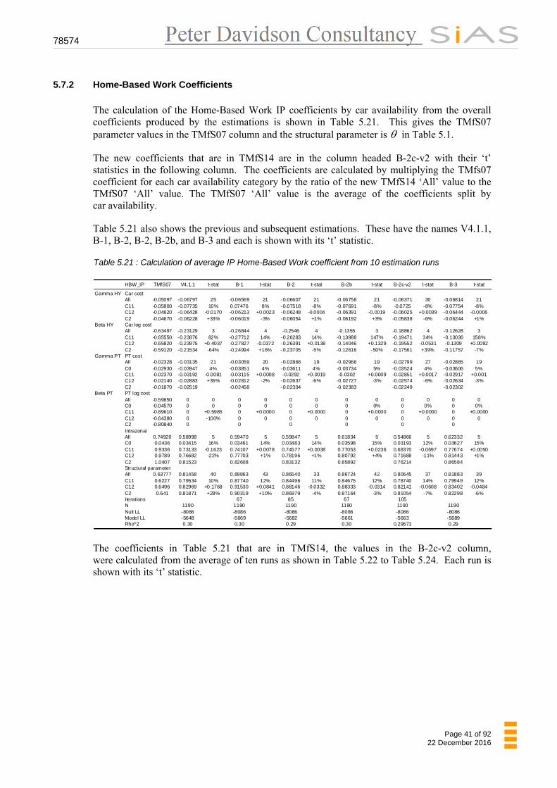
78574
Page 41 of 92 22 December 2016
5.7.2 Home-Based Work Coefficients
The calculation of the Home-Based Work IP coefficients by car availability from the overall coefficients produced by the estimations is shown in Table 5.21. This gives the TMfS07 parameter values in the TMfS07 column and the structural parameter is in Table 5.1.
The new coefficients that are in TMfS14 are in the column headed B-2c-v2 with their ‘t’ statistics in the following column. The coefficients are calculated by multiplying the TMfs07 coefficient for each car availability category by the ratio of the new TMfS14 ‘All’ value to the TMfS07 ‘All’ value. The TMfS07 ‘All’ value is the average of the coefficients split by car availability.
Table 5.21 also shows the previous and subsequent estimations. These have the names V4.1.1, B-1, B-2, B-2, B-2b, and B-3 and each is shown with its ‘t’ statistic.
Table 5.21 : Calculation of average IP Home-Based Work coefficient from 10 estimation runs
HBW_IP TMfS07 V4.1.1 t-stat B-1 t-stat B-2 t-stat B-2b t-stat B-2c-v2 t-stat B-3 t-stat
Gamma HY Car costAll -0.05097 -0.06797 25 -0.06569 21 -0.06607 21 -0.06758 21 -0.06371 30 -0.06814 21C11 -0.05800 -0.07735 10% 0.07476 8% -0.07518 -8% -0.07691 -8% -0.0725 -8% -0.07754 -8%C12 -0.04820 -0.06428 -0.0170 -0.06213 +0.0023 -0.06248 -0.0004 -0.06391 -0.0019 -0.06025 +0.0039 -0.06444 -0.0006C2 -0.04670 -0.06228 +33% -0.06019 -3% -0.06054 +1% -0.06192 +3% -0.05838 -6% -0.06244 +1%
Beta HY Car log costAll -0.63497 -0.23129 3 -0.26844 4 -0.2546 4 -0.1355 3 -0.18862 4 -0.12628 3C11 -0.65550 -0.23876 82% -0.27712 14% -0.26283 14% -0.13988 147% -0.19471 34% -0.13036 158%C12 -0.65820 -0.23975 +0.4037 -0.27827 -0.0372 -0.26391 +0.0138 -0.14046 +0.1329 -0.19552 -0.0531 -0.1309 +0.0092C2 -0.59120 -0.21534 -64% -0.24994 +16% -0.23705 -5% -0.12616 -50% -0.17561 +39% -0.11757 -7%
Gamma PT PT costAll -0.02328 -0.03135 21 -0.03059 20 -0.02868 19 -0.02966 19 -0.02799 27 -0.02865 19C0 -0.02930 -0.03947 4% -0.03851 4% -0.03611 4% -0.03734 5% -0.03524 4% -0.03606 5%C11 -0.02370 -0.03192 -0.0081 -0.03115 +0.0008 -0.0292 +0.0019 -0.0302 +0.0009 -0.02851 +0.0017 -0.02917 +0.001C12 -0.02140 -0.02883 +35% -0.02812 -2% -0.02637 -6% -0.02727 -3% -0.02574 -6% -0.02634 -3%C2 -0.01870 -0.02519 -0.02458 -0.02304 -0.02383 -0.02249 -0.02302
Beta PT PT log costAll -0.59850 0 0 0 0 0 0 0 0 0 0 0 0C0 -0.04570 0 0 0 0 0 0 0 0% 0 0% 0 0%C11 -0.89610 0 +0.5985 0 +0.0000 0 +0.0000 0 +0.0000 0 +0.0000 0 +0.0000C12 -0.64380 0 -100% 0 0 0 0 0 0 0 0 0 0C2 -0.80840 0 0 0 0 0 0IntrazonalAll 0.74920 0.58998 5 0.59470 5 0.59847 5 0.61834 5 0.54866 5 0.62332 5C0 0.0436 0.03415 16% 0.03461 14% 0.03483 14% 0.03598 15% 0.03193 12% 0.03627 15%C11 0.9336 0.73133 -0.1623 0.74107 +0.0078 0.74577 +0.0038 0.77053 +0.0236 0.68370 -0.0697 0.77674 +0.0050C12 0.9789 0.76682 -22% 0.77703 +1% 0.78196 +1% 0.80792 +4% 0.71688 -11% 0.81443 +1%C2 1.0407 0.81523 0.82608 0.83132 0.85892 0.76214 0.86584Structural parameterAll 0.63777 0.81458 40 0.89863 43 0.86540 33 0.86724 42 0.80645 37 0.81883 39C11 0.6227 0.79534 10% 0.87740 12% 0.84496 11% 0.84675 12% 0.78740 14% 0.79949 12%C12 0.6496 0.82969 +0.1768 0.91530 +0.0841 0.88146 -0.0332 0.88333 -0.0314 0.82141 -0.0608 0.83402 -0.0484C2 0.641 0.81871 +28% 0.90319 +10% 0.86979 -4% 0.87164 -3% 0.81054 -7% 0.82298 -6%Iterations 67 85 67 105N 1190 1190 1190 1190 1190 1190Null LL -8086 -8086 -8086 -8086 -8086 -8086Model LL -5648 -5669 -5682 -5661 -5663 -5689Rho^2 0.30 0.30 0.29 0.30 0.29673 0.29
The coefficients in Table 5.21 that are in TMfS14, the values in the B-2c-v2 column, were calculated from the average of ten runs as shown in Table 5.22 to Table 5.24. Each run is shown with its ‘t’ statistic.
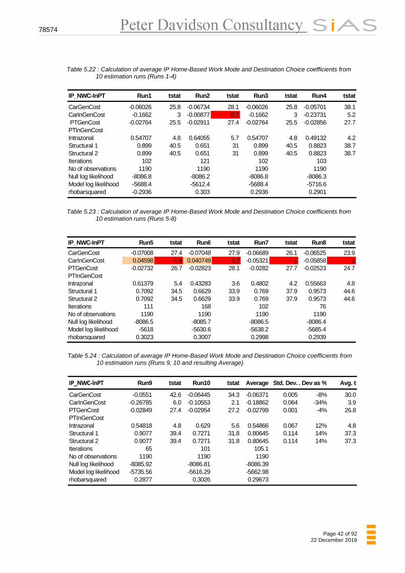
78574
Page 42 of 92 22 December 2016
Table 5.22 : Calculation of average IP Home-Based Work Mode and Destination Choice coefficients from
10 estimation runs (Runs 1-4)
IP_NWC-InPT Run1 tstat Run2 tstat Run3 tstat Run4 tstat
CarGenCost -0.06026 25.8 -0.06734 28.1 -0.06026 25.8 -0.05701 38.1CarlnGenCost -0.1662 3 -0.00877 0.2 -0.1662 3 -0.23731 5.2 PTGenCost -0.02764 25.5 -0.02911 27.4 -0.02764 25.5 -0.02856 27.7PTlnGenCostIntrazonal 0.54707 4.8 0.64055 5.7 0.54707 4.8 0.49132 4.2Structural 1 0.899 40.5 0.651 31 0.899 40.5 0.8823 38.7Structural 2 0.899 40.5 0.651 31 0.899 40.5 0.8823 38.7Iterations 102 121 102 103 No of observations 1190 1190 1190 1190 Null log likelihood -8086.8 -8086.2 -8086.8 -8086.3 Model log likelihood -5688.4 -5612.4 -5688.4 -5716.6 rhobarsquared -0.2936 0.303 0.2936 0.2901
Table 5.23 : Calculation of average IP Home-Based Work Mode and Destination Choice coefficients from 10 estimation runs (Runs 5-8)
IP_NWC-InPT Run5 tstat Run6 tstat Run7 tstat Run8 tstat
CarGenCost -0.07008 27.4 -0.07048 27.9 -0.06689 26.1 -0.06525 23.9CarInGenCost 0.04598 0.8 0.040749 0.7 -0.05321 1 -0.05858 1PTGenCost -0.02732 26.7 -0.02823 28.1 -0.0282 27.7 -0.02523 24.7PTInGenCostIntrazonal 0.61379 5.4 0.43283 3.6 0.4802 4.2 0.55663 4.8Structural 1 0.7092 34.5 0.6629 33.9 0.769 37.9 0.9573 44.6Structural 2 0.7092 34.5 0.6629 33.9 0.769 37.9 0.9573 44.6Iterations 111 168 102 76No of observations 1190 1190 1190 1190Null log likelihood -8086.5 -8085.7 -8086.5 -8086.4Model log likelihood -5618 -5630.6 -5638.2 -5685.4rhobarsquared 0.3023 0.3007 0.2998 0.2939
Table 5.24 : Calculation of average IP Home-Based Work Mode and Destination Choice coefficients from 10 estimation runs (Runs 9, 10 and resulting Average)
IP_NWC-lnPT Run9 tstat Run10 tstat Average Std. Dev. . Dev as % Avg. t
CarGenCost -0.0551 42.6 -0.06445 34.3 -0.06371 0.005 -8% 30.0CarInGenCost -0.26785 6.0 -0.10553 2.1 -0.18862 0.064 -34% 3.9PTGenCost -0.02849 27.4 -0.02954 27.2 -0.02799 0.001 -4% 26.8PTInGenCostIntrazonal 0.54818 4.8 0.629 5.6 0.54866 0.067 12% 4.8Structural 1 0.9077 39.4 0.7271 31.8 0.80645 0.114 14% 37.3Structural 2 0.9077 39.4 0.7271 31.8 0.80645 0.114 14% 37.3Iterations 65 101 105.1No of observations 1190 1190 1190Null log likelihood -8085.92 -8086.81 -8086.39Model log likelihood -5735.56 -5616.29 -5662.98rhobarsquared 0.2877 0.3026 0.29673
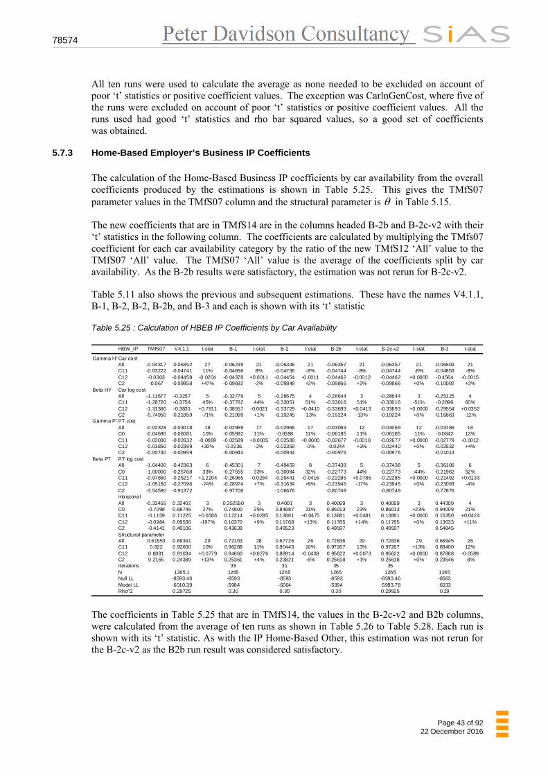
78574
Page 43 of 92 22 December 2016
All ten runs were used to calculate the average as none needed to be excluded on account of poor ‘t’ statistics or positive coefficient values. The exception was CarlnGenCost, where five of the runs were excluded on account of poor ‘t’ statistics or positive coefficient values. All the runs used had good ‘t’ statistics and rho bar squared values, so a good set of coefficients was obtained.
5.7.3 Home-Based Employer’s Business IP Coefficients
The calculation of the Home-Based Business IP coefficients by car availability from the overall coefficients produced by the estimations is shown in Table 5.25. This gives the TMfS07 parameter values in the TMfS07 column and the structural parameter is in Table 5.15.
The new coefficients that are in TMfS14 are in the columns headed B-2b and B-2c-v2 with their ‘t’ statistics in the following column. The coefficients are calculated by multiplying the TMfs07 coefficient for each car availability category by the ratio of the new TMfS12 ‘All’ value to the TMfS07 ‘All’ value. The TMfS07 ‘All’ value is the average of the coefficients split by car availability. As the B-2b results were satisfactory, the estimation was not rerun for B-2c-v2.
Table 5.11 also shows the previous and subsequent estimations. These have the names V4.1.1, B-1, B-2, B-2, B-2b, and B-3 and each is shown with its ‘t’ statistic
Table 5.25 : Calculation of HBEB IP Coefficients by Car Availability
HBW_IP TMfS07 V4.1.1 t-stat B-1 t-stat B-2 t-stat B-2b t-stat B-2c-v2 t-stat B-3 t-stat
Gamma HYCar costAll -0.04317 -0.06352 27 -0.06239 21 -0.06346 21 -0.06357 21 -0.06357 21 -0.06503 21C11 -0.03222 -0.04741 11% -0.04656 8% -0.04736 -8% -0.04744 -8% -0.04744 -8% -0.04853 -8%C12 -0.0303 -0.04458 -0.0204 -0.04378 +0.0011 -0.04454 -0.0011 -0.04462 -0.0012 -0.04462 +0.0000 -0.4564 -0.0015C2 -0.067 -0.09858 +47% -0.09682 -2% -0.09848 +2% -0.09866 +2% -0.09866 +0% -0.10092 +2%
Beta HY Car log costAll -1.11677 -0.3257 5 -0.32779 5 -0.28675 4 -0.28644 3 -0.28644 3 -0.25125 4C11 -1.28720 -0.3754 45% -0.37782 44% -0.33051 51% -0.33016 51% -0.33016 -51% -0.2896 60%C12 -1.31360 -0.3831 +0.7911 -0.38557 -0.0021 -0.33729 +0.0410 -0.33693 +0.0413 -0.33693 +0.0000 -0.29554 +0.0352C2 -0.74950 -0.21859 -71% -0.21999 +1% -0.19245 -13% -0.19224 -13% -0.19224 +0% -0.16863 -12%
Gamma PTPT costAll -0.02328 -0.03018 18 -0.02969 17 -0.02968 17 -0.03069 12 -0.03069 12 -0.03186 18C0 -0.04690 -0.06081 10% -0.05982 11% -0.0598 11% -0.06185 11% -0.06185 -11% -0.0642 12%C11 -0.02030 -0.02632 -0.0069 -0.02589 +0.0005 -0.02588 +0.0000 -0.02677 -0.0010 -0.02677 +0.0000 -0.02779 -0.0012C12 -0.01850 -0.02399 +30% -0.0236 -2% -0.02359 -0% -0.0244 +3% -0.02440 +0% -0.02532 +4%C2 -0.00740 -0.00959 -0.00944 -0.00944 -0.00976 -0.00976 -0.01013
Beta PT PT log costAll -1.64400 -0.42363 6 -0.45301 7 -0.49459 8 -0.37438 5 -0.37438 5 -0.36106 6C0 -1.00000 -0.25768 33% -0.27555 33% -0.30084 32% -0.22773 44% -0.22773 -44% -0.21962 52%C11 -0.97860 -0.25217 +1.2204 -0.26965 -0.0294 -0.29441 -0.0416 -0.22285 +0.0786 -0.22285 +0.0000 -0.21492 +0.0133C12 -1.05150 -0.27096 -74% -0.28974 +7% -0.31634 +9% -0.23945 -17% -0.23945 +0% -0.23093 -4%C2 -3.54590 -0.91372 -0.97708 -1.06676 -0.80749 -0.80749 -0.77876IntrazonalAll -0.33455 0.32402 3 0.352550 3 0.4001 3 0.40069 3 0.40069 3 0.44309 4C0 -0.7098 0.68746 27% 0.74800 25% 0.84887 23% 0.85013 23% 0.85013 +23% 0.94009 21%C11 -0.1159 0.11225 +0.6586 0.12214 +0.0285 0.13861 +0.0475 0.13881 +0.0481 0.13881 +0.0000 0.15350 +0.0424C12 -0.0984 0.09530 -197% 0.10370 +9% 0.11768 +13% 0.11785 +14% 0.11785 +0% 0.13033 +11%C2 -0.4141 0.40106 0.43639 0.49523 0.49597 0.49597 0.54845Structural parameterAll 0.61553 0.69341 29 0.72103 28 0.67726 26 0.72836 29 0.72836 29 0.66945 26C11 0.822 0.92600 10% 0.96288 11% 0.90443 10% 0.97267 13% 0.97267 +13% 0.89400 12%C12 0.8081 0.91034 +0.0779 0.94660 +0.0276 0.88914 -0.0438 0.95622 +0.0073 0.95622 +0.0000 0.87888 -0.0589C2 0.2165 0.24389 +13% 0.25361 +4% 0.23821 -6% 0.25618 +1% 0.25618 +0% 0.23546 -8%Iterations 35 31 35 35N 1265.1 1265 1265 1265 1265 1265Null LL -8593.46 -8593 -8593 -8593 -8593.46 -8563Model LL -6010.39 -5984 -6004 -5994 -5993.78 -6033Rho^2 0.29725 0.30 0.30 0.30 0.29925 0.29
The coefficients in Table 5.25 that are in TMfS14, the values in the B-2c-v2 and B2b columns, were calculated from the average of ten runs as shown in Table 5.26 to Table 5.28. Each run is shown with its ‘t’ statistic. As with the IP Home-Based Other, this estimation was not rerun for the B-2c-v2 as the B2b run result was considered satisfactory.
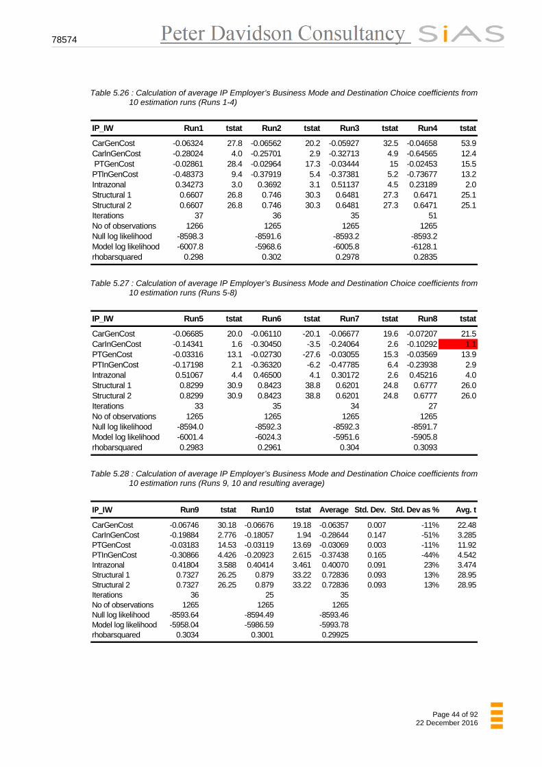
78574
Page 44 of 92 22 December 2016
Table 5.26 : Calculation of average IP Employer’s Business Mode and Destination Choice coefficients from
10 estimation runs (Runs 1-4)
IP_IW Run1 tstat Run2 tstat Run3 tstat Run4 tstat
CarGenCost -0.06324 27.8 -0.06562 20.2 -0.05927 32.5 -0.04658 53.9CarlnGenCost -0.28024 4.0 -0.25701 2.9 -0.32713 4.9 -0.64565 12.4 PTGenCost -0.02861 28.4 -0.02964 17.3 -0.03444 15 -0.02453 15.5PTlnGenCost -0.48373 9.4 -0.37919 5.4 -0.37381 5.2 -0.73677 13.2Intrazonal 0.34273 3.0 0.3692 3.1 0.51137 4.5 0.23189 2.0Structural 1 0.6607 26.8 0.746 30.3 0.6481 27.3 0.6471 25.1Structural 2 0.6607 26.8 0.746 30.3 0.6481 27.3 0.6471 25.1Iterations 37 36 35 51No of observations 1266 1265 1265 1265Null log likelihood -8598.3 -8591.6 -8593.2 -8593.2Model log likelihood -6007.8 -5968.6 -6005.8 -6128.1rhobarsquared 0.298 0.302 0.2978 0.2835
Table 5.27 : Calculation of average IP Employer’s Business Mode and Destination Choice coefficients from
10 estimation runs (Runs 5-8)
IP_IW Run5 tstat Run6 tstat Run7 tstat Run8 tstat
CarGenCost -0.06685 20.0 -0.06110 -20.1 -0.06677 19.6 -0.07207 21.5CarInGenCost -0.14341 1.6 -0.30450 -3.5 -0.24064 2.6 -0.10292 1.1PTGenCost -0.03316 13.1 -0.02730 -27.6 -0.03055 15.3 -0.03569 13.9PTInGenCost -0.17198 2.1 -0.36320 -6.2 -0.47785 6.4 -0.23938 2.9Intrazonal 0.51067 4.4 0.46500 4.1 0.30172 2.6 0.45216 4.0Structural 1 0.8299 30.9 0.8423 38.8 0.6201 24.8 0.6777 26.0Structural 2 0.8299 30.9 0.8423 38.8 0.6201 24.8 0.6777 26.0Iterations 33 35 34 27No of observations 1265 1265 1265 1265Null log likelihood -8594.0 -8592.3 -8592.3 -8591.7Model log likelihood -6001.4 -6024.3 -5951.6 -5905.8rhobarsquared 0.2983 0.2961 0.304 0.3093
Table 5.28 : Calculation of average IP Employer’s Business Mode and Destination Choice coefficients from
10 estimation runs (Runs 9, 10 and resulting average)
IP_IW Run9 tstat Run10 tstat Average Std. Dev. Std. Dev as % Avg. t
CarGenCost -0.06746 30.18 -0.06676 19.18 -0.06357 0.007 -11% 22.48CarInGenCost -0.19884 2.776 -0.18057 1.94 -0.28644 0.147 -51% 3.285PTGenCost -0.03183 14.53 -0.03119 13.69 -0.03069 0.003 -11% 11.92PTInGenCost -0.30866 4.426 -0.20923 2.615 -0.37438 0.165 -44% 4.542Intrazonal 0.41804 3.588 0.40414 3.461 0.40070 0.091 23% 3.474Structural 1 0.7327 26.25 0.879 33.22 0.72836 0.093 13% 28.95Structural 2 0.7327 26.25 0.879 33.22 0.72836 0.093 13% 28.95Iterations 36 25 35No of observations 1265 1265 1265Null log likelihood -8593.64 -8594.49 -8593.46Model log likelihood -5958.04 -5986.59 -5993.78rhobarsquared 0.3034 0.3001 0.29925

78574
Page 45 of 92 22 December 2016
All ten runs were used to calculate the average as none needed to be excluded on account of poor ‘t’ statistics or positive coefficient values except for Run 8 CarinGenCost, which had a poor ‘t’ stat. All the other ‘t’ statistics and rho bar squared vales were acceptable, so an acceptable set of coefficients was obtained.

78574
Page 46 of 92 22 December 2016

78574
Page 47 of 92 22 December 2016
6 OTHER UPDATES
The vehicle occupancy matrices were updated to be in line with the trends from the November 2014 WebTAG guidance (November 2014 – webtag-data-boook-may2014.xlm), sheet A1.3.3.
New Park & Ride sites with their capacities and costs (where appropriate) were added to the Park & Rite site file with their transfer times set to zero. The Park & Ride model was run for one iteration and the resulting calculated transfer times were set as the base transfer times.
6.1 New incremental matrices
TMfS14 makes use of incremental matrices which are an adjustment applied to the synthetic matrices output from the mode and destination choice and reverse factoring processes.
The base year validated matrices were accepted as the best representation of the base year travel pattern and so the incremental matrices are conceptually the ‘correction’ required to arrive at these matrices from a starting point of the synthetic base year matrices produced by the demand model.
The incremental matrices remain constant for all model runs and the same adjustment or ‘correction’ is applied to the forecast year synthesised trip matrices which are produced by forecast runs of the Demand Model.
As part of the TMfS14 update the new incremental matrices were developed such that, when run for 2014, the trip matrices output by the first iteration of the demand model match precisely the validated 2014 base year assignment matrices.
The cells of the incremental matrices were generated in one of two ways:
Case 1 bf SBSF
Case 2
bf S
BSF *
Where B Base observed trips
bS Base modelled (synthesised) trips
fS Future modelled (synthesised) trips
F Future Trips
The following cases were defined when creating or applying the incremental matrices:
Case 1: Was used where B is zero or where we have high B and low Sb, defined as the case where B/Sb>2.

78574
Page 48 of 92 22 December 2016
Case 2: Was used in the following circumstances:
Low B, high Sb
Low B low Sb
High B high Sb
This allowed zero cells in the base year to be incremented using Case 1 and avoids applying high multiplicative factors. The bracketed terms above form the incremental matrices. The equations show how they are applied in forecasting.
6.2 Park & Ride model update
The inputs to the site choice calibration are the Park & Ride generalised costs and Park & Ride sites. Each site file contains a specification of the site catchment area, which are defined as a list of zones, which in nearly every case are all other zones.
The site file also contains the Car Park Charge (if any) and the number of ‘official’ car parking spaces.
Note the Park & Ride station choice model allows users to park outside the ‘official’ car parking spaces, as is the reality at a number of stations.
Each Park & Ride site also has a calibrated transfer time, which is added to the generalised costs within the car park choice process and is specified in the site file. The transfer time aims to reflect a variety of attributes of the Park & Ride site (e.g. cleanliness, ease of transfer, security etc.) and is used as a calibration tool. This parameter does not vary with car park occupancy.
The TMfS14 update of the Park and Ride model was primarily the inclusion of thirty nine additional Park & Ride sites along with any changes to the number of parking spaces at each site. The change in the TMfS14 zone system was also incorporated into the park and ride model inputs. The TMfS12 observed Park & Ride data was not updated as part of the TMfS14 development and no observed data for the additional park and ride sites was available within the timescales of the model development.
Table 6.1 shows the total usage of Park & Ride Sites by Local Authority. The new TMfS14 sites were not included as there was insufficient time to include observed data. The total observed trips is in vehicles. The modelled total is calculated from the period person matrices, but with an average occupancy of 1.2 applied. The calibration of each Park & Ride site by journey purpose is included in Appendix D.
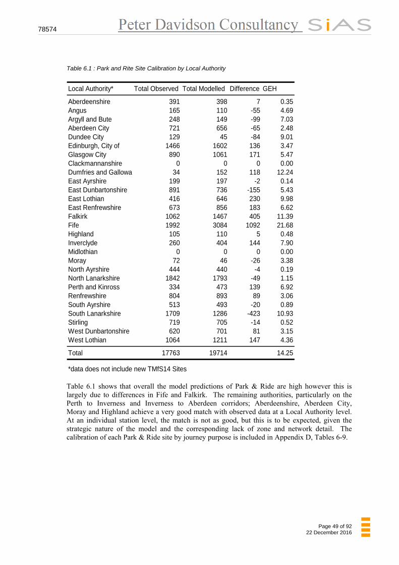
78574
Page 49 of 92 22 December 2016
Table 6.1 : Park and Rite Site Calibration by Local Authority
Local Authority* Total Observed Total Modelled Difference GEH
Aberdeenshire 391 398 7 0.35Angus 165 110 -55 4.69Argyll and Bute 248 149 -99 7.03Aberdeen City 721 656 -65 2.48Dundee City 129 45 -84 9.01Edinburgh, City of 1466 1602 136 3.47Glasgow City 890 1061 171 5.47Clackmannanshire 0 0 0 0.00Dumfries and Galloway 34 152 118 12.24East Ayrshire 199 197 -2 0.14East Dunbartonshire 891 736 -155 5.43East Lothian 416 646 230 9.98East Renfrewshire 673 856 183 6.62Falkirk 1062 1467 405 11.39Fife 1992 3084 1092 21.68Highland 105 110 5 0.48Inverclyde 260 404 144 7.90Midlothian 0 0 0 0.00Moray 72 46 -26 3.38North Ayrshire 444 440 -4 0.19North Lanarkshire 1842 1793 -49 1.15Perth and Kinross 334 473 139 6.92Renfrewshire 804 893 89 3.06South Ayrshire 513 493 -20 0.89South Lanarkshire 1709 1286 -423 10.93Stirling 719 705 -14 0.52West Dunbartonshire 620 701 81 3.15West Lothian 1064 1211 147 4.36
Total 17763 19714 14.25
*data does not include new TMfS14 Sites
Table 6.1 shows that overall the model predictions of Park & Ride are high however this is largely due to differences in Fife and Falkirk. The remaining authorities, particularly on the Perth to Inverness and Inverness to Aberdeen corridors; Aberdeenshire, Aberdeen City, Moray and Highland achieve a very good match with observed data at a Local Authority level. At an individual station level, the match is not as good, but this is to be expected, given the strategic nature of the model and the corresponding lack of zone and network detail. The calibration of each Park & Ride site by journey purpose is included in Appendix D, Tables 6-9.

78574
Page 50 of 92 22 December 2016
78574
Page 51 of 92 22 December 2016
7 SENSITIVITY TESTS
7.1 Introduction
The sensitivity tests were run in accordance with the guidance in the DfT’s TAG unit M2 Variable Demand Modelling (January 2014), which recommends checking the elasticity of demand with respect to:
Road fuel price
Public transport fares
Road journey time
The demand model runs that were undertaken to test these responses were as follows:
10% increase in fuel cost
10% increase in PT fares
10% increase in Road journey times
The rest of the parameters were kept unchanged. External and long distance trips were excluded from the tests and all others were included. For the car fuel cost sensitivity tests, the elasticities were calculated by weighting the trips by distance to get vehicle kilometres. For Road journey time and PT fares, the number of trips were used, as required by WebTAG.
The method for calculating the elasticity is shown below using car fuel prices as an example, where C and C’ are the base and test car fuel prices (indices), and K and K’ are the base and test car vehicle kilometres.
The elasticities were calculated using:
CC
kke
ln'ln
ln'ln
This ensured that the elasticity was a good approximation to the point elasticity at the midpoint of the data.
7.2 Results
The results are firstly given at an aggregate level and then split by time period and purpose. The elasticities are also reported separately for journeys that are in the A9/A96 corridor (identified as a corridor of particular interest) and those that are not, with the combined results also given. Commentary on the results is given in Section 8.4.
The results are also given in two separate sets: one set calculated using the trip matrices just before inclusion of external trips and application of the incremental matrices (in the Assignment Prep module), and the other set calculated directly after the Mode and Destination Choice application. While the latter set are not required for review against WebTAG, they are included to help illustrate how the model responds. Finally, a brief overall summary of the outcome of the realism tests is included after the results.
The following table is based on WebTAG’s summary (Table 6.2, TAG Unit M2, January 2014) of the recommended elasticity ranges for the three realism tests.
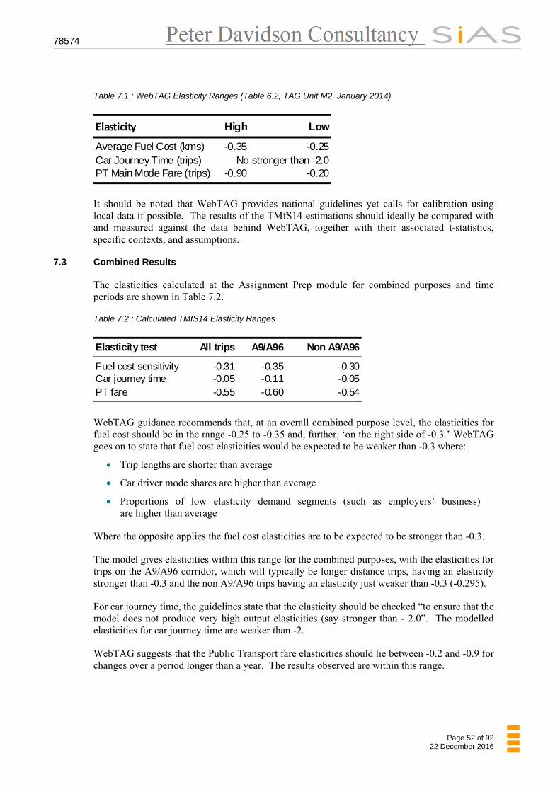
78574
Page 52 of 92 22 December 2016
Table 7.1 : WebTAG Elasticity Ranges (Table 6.2, TAG Unit M2, January 2014)
Elasticity High Low
Average Fuel Cost (kms) -0.35 -0.25Car Journey Time (trips)PT Main Mode Fare (trips) -0.90 -0.20
No stronger than -2.0
It should be noted that WebTAG provides national guidelines yet calls for calibration using local data if possible. The results of the TMfS14 estimations should ideally be compared with and measured against the data behind WebTAG, together with their associated t-statistics, specific contexts, and assumptions.
7.3 Combined Results
The elasticities calculated at the Assignment Prep module for combined purposes and time periods are shown in Table 7.2.
Table 7.2 : Calculated TMfS14 Elasticity Ranges
Elasticity test All trips A9/A96 Non A9/A96
Fuel cost sensitivity -0.31 -0.35 -0.30Car journey time -0.05 -0.11 -0.05PT fare -0.55 -0.60 -0.54
WebTAG guidance recommends that, at an overall combined purpose level, the elasticities for fuel cost should be in the range -0.25 to -0.35 and, further, ‘on the right side of -0.3.’ WebTAG goes on to state that fuel cost elasticities would be expected to be weaker than -0.3 where:
Trip lengths are shorter than average
Car driver mode shares are higher than average
Proportions of low elasticity demand segments (such as employers’ business) are higher than average
Where the opposite applies the fuel cost elasticities are to be expected to be stronger than -0.3.
The model gives elasticities within this range for the combined purposes, with the elasticities for trips on the A9/A96 corridor, which will typically be longer distance trips, having an elasticity stronger than -0.3 and the non A9/A96 trips having an elasticity just weaker than -0.3 (-0.295).
For car journey time, the guidelines state that the elasticity should be checked “to ensure that the model does not produce very high output elasticities (say stronger than - 2.0”. The modelled elasticities for car journey time are weaker than -2.
WebTAG suggests that the Public Transport fare elasticities should lie between -0.2 and -0.9 for changes over a period longer than a year. The results observed are within this range.
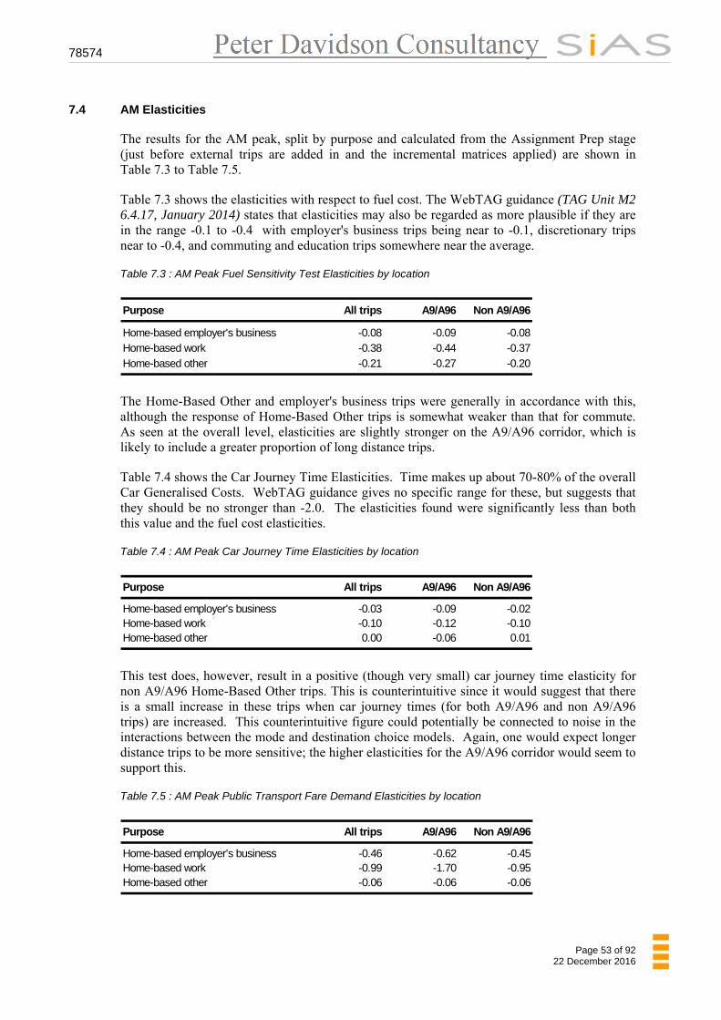
78574
Page 53 of 92 22 December 2016
7.4 AM Elasticities
The results for the AM peak, split by purpose and calculated from the Assignment Prep stage (just before external trips are added in and the incremental matrices applied) are shown in Table 7.3 to Table 7.5.
Table 7.3 shows the elasticities with respect to fuel cost. The WebTAG guidance (TAG Unit M2 6.4.17, January 2014) states that elasticities may also be regarded as more plausible if they are in the range -0.1 to -0.4 with employer's business trips being near to -0.1, discretionary trips near to -0.4, and commuting and education trips somewhere near the average.
Table 7.3 : AM Peak Fuel Sensitivity Test Elasticities by location
Purpose All trips A9/A96 Non A9/A96
Home-based employer's business -0.08 -0.09 -0.08Home-based work -0.38 -0.44 -0.37Home-based other -0.21 -0.27 -0.20
The Home-Based Other and employer's business trips were generally in accordance with this, although the response of Home-Based Other trips is somewhat weaker than that for commute. As seen at the overall level, elasticities are slightly stronger on the A9/A96 corridor, which is likely to include a greater proportion of long distance trips.
Table 7.4 shows the Car Journey Time Elasticities. Time makes up about 70-80% of the overall Car Generalised Costs. WebTAG guidance gives no specific range for these, but suggests that they should be no stronger than -2.0. The elasticities found were significantly less than both this value and the fuel cost elasticities.
Table 7.4 : AM Peak Car Journey Time Elasticities by location
Purpose All trips A9/A96 Non A9/A96
Home-based employer's business -0.03 -0.09 -0.02Home-based work -0.10 -0.12 -0.10Home-based other 0.00 -0.06 0.01
This test does, however, result in a positive (though very small) car journey time elasticity for non A9/A96 Home-Based Other trips. This is counterintuitive since it would suggest that there is a small increase in these trips when car journey times (for both A9/A96 and non A9/A96 trips) are increased. This counterintuitive figure could potentially be connected to noise in the interactions between the mode and destination choice models. Again, one would expect longer distance trips to be more sensitive; the higher elasticities for the A9/A96 corridor would seem to support this.
Table 7.5 : AM Peak Public Transport Fare Demand Elasticities by location
Purpose All trips A9/A96 Non A9/A96
Home-based employer's business -0.46 -0.62 -0.45Home-based work -0.99 -1.70 -0.95Home-based other -0.06 -0.06 -0.06
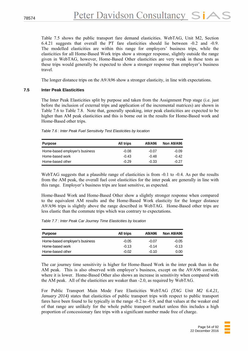
78574
Page 54 of 92 22 December 2016
Table 7.5 shows the public transport fare demand elasticities. WebTAG, Unit M2, Section 6.4.21 suggests that overall the PT fare elasticities should lie between -0.2 and -0.9. The modelled elasticities are within this range for employers’ business trips, while the elasticities for all Home-Based Work trips show a stronger response, slightly outside the range given in WebTAG, however, Home-Based Other elasticities are very weak in these tests as these trips would generally be expected to show a stronger response than employer’s business travel.
The longer distance trips on the A9/A96 show a stronger elasticity, in line with expectations.
7.5 Inter Peak Elasticities
The Inter Peak Elasticities split by purpose and taken from the Assignment Prep stage (i.e. just before the inclusion of external trips and application of the incremental matrices) are shown in Table 7.6 to Table 7.8. Note that, generally speaking, inter peak elasticities are expected to be higher than AM peak elasticities and this is borne out in the results for Home-Based work and Home-Based other trips.
Table 7.6 : Inter Peak Fuel Sensitivity Test Elasticities by location
Purpose All trips A9/A96 Non A9/A96
Home-based employer's business -0.08 -0.07 -0.09Home-based work -0.43 -0.48 -0.42Home-based other -0.29 -0.33 -0.27
WebTAG suggests that a plausible range of elasticities is from -0.1 to -0.4. As per the results from the AM peak, the overall fuel cost elasticities for the inter peak are generally in line with this range. Employer’s business trips are least sensitive, as expected.
Home-Based Work and Home-Based Other show a slightly stronger response when compared to the equivalent AM results and the Home-Based Work elasticity for the longer distance A9/A96 trips is slightly above the range described in WebTAG. Home-Based other trips are less elastic than the commute trips which was contrary to expectations.
Table 7.7 : Inter Peak Car Journey Time Elasticities by location
Purpose All trips A9/A96 Non A9/A96
Home-based employer's business -0.05 -0.07 -0.05Home-based work -0.13 -0.14 -0.13Home-based other -0.02 -0.10 0.00
The car journey time sensitivity is higher for Home-Based Work in the inter peak than in the AM peak. This is also observed with employer’s business, except on the A9/A96 corridor, where it is lower. Home-Based Other also shows an increase in sensitivity when compared with the AM peak. All of the elasticities are weaker than -2.0, as required by WebTAG.
For Public Transport Main Mode Fare Elasticities WebTAG (TAG Unit M2 6.4.21, January 2014) states that elasticities of public transport trips with respect to public transport fares have been found to lie typically in the range -0.2 to -0.9, and that values at the weaker end of that range are unlikely for the whole public transport market unless this includes a high proportion of concessionary fare trips with a significant number made free of charge.
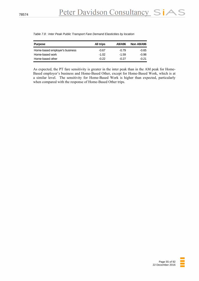
78574
Page 55 of 92 22 December 2016
Table 7.8 : Inter Peak Public Transport Fare Demand Elasticities by location
Purpose All trips A9/A96 Non A9/A96
Home-based employer's business -0.67 -0.79 -0.65Home-based work -1.02 -1.59 -0.98Home-based other -0.22 -0.27 -0.21
As expected, the PT fare sensitivity is greater in the inter peak than in the AM peak for Home-Based employer’s business and Home-Based Other, except for Home-Based Work, which is at a similar level. The sensitivity for Home-Based Work is higher than expected, particularly when compared with the response of Home-Based Other trips.

78574
Page 56 of 92 22 December 2016
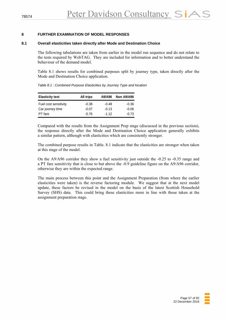
78574
Page 57 of 92 22 December 2016
8 FURTHER EXAMINATION OF MODEL RESPONSES
8.1 Overall elasticities taken directly after Mode and Destination Choice
The following tabulations are taken from earlier in the model run sequence and do not relate to the tests required by WebTAG. They are included for information and to better understand the behaviour of the demand model.
Table 8.1 shows results for combined purposes split by journey type, taken directly after the Mode and Destination Choice application.
Table 8.1 : Combined Purpose Elasticities by Journey Type and location
Elasticity test All trips A9/A96 Non A9/A96
Fuel cost sensitivity -0.38 -0.48 -0.36Car journey time -0.07 -0.13 -0.06PT fare -0.76 -1.12 -0.73
Compared with the results from the Assignment Prep stage (discussed in the previous section), the response directly after the Mode and Destination Choice application generally exhibits a similar pattern, although with elasticities which are consistently stronger.
The combined purpose results in Table. 8.1 indicate that the elasticities are stronger when taken at this stage of the model.
On the A9/A96 corridor they show a fuel sensitivity just outside the -0.25 to -0.35 range and a PT fare sensitivity that is close to but above the -0.9 guideline figure on the A9/A96 corridor, otherwise they are within the expected range.
The main process between this point and the Assignment Preparation (from where the earlier elasticities were taken) is the reverse factoring module. We suggest that at the next model update, these factors be revised in the model on the basis of the latest Scottish Household Survey (SHS) data. This could bring these elasticities more in line with those taken at the assignment preparation stage.
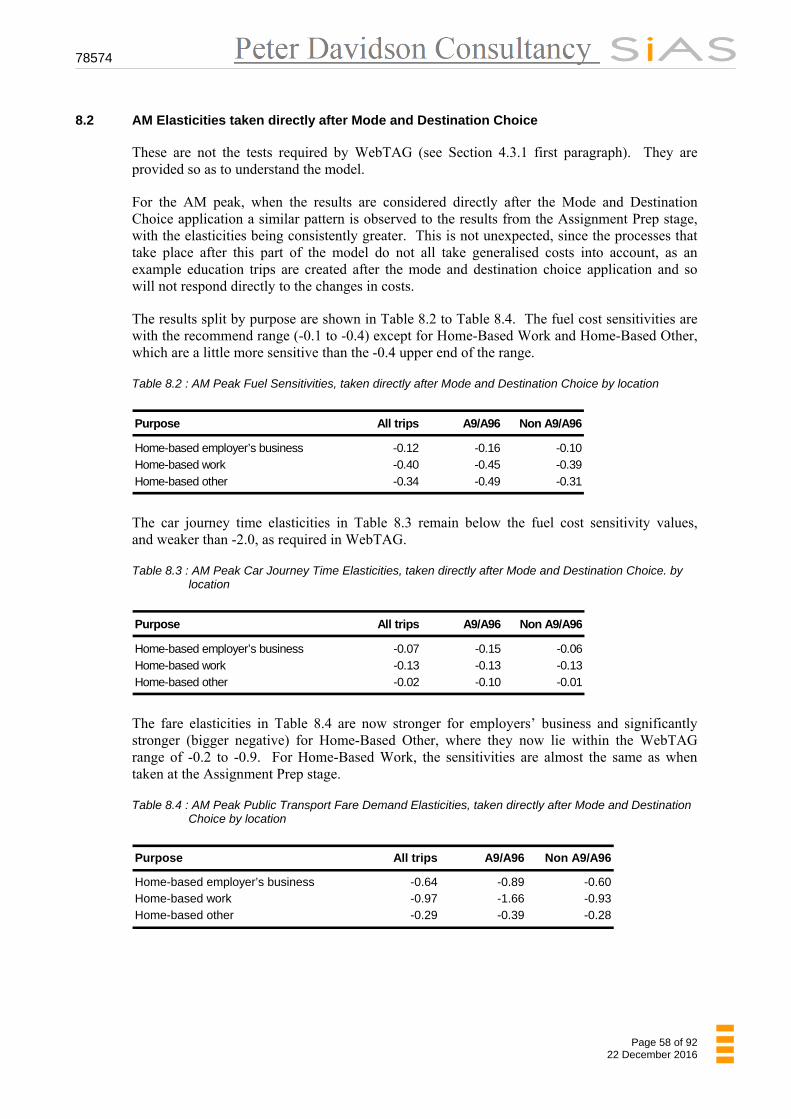
78574
Page 58 of 92 22 December 2016
8.2 AM Elasticities taken directly after Mode and Destination Choice
These are not the tests required by WebTAG (see Section 4.3.1 first paragraph). They are provided so as to understand the model.
For the AM peak, when the results are considered directly after the Mode and Destination Choice application a similar pattern is observed to the results from the Assignment Prep stage, with the elasticities being consistently greater. This is not unexpected, since the processes that take place after this part of the model do not all take generalised costs into account, as an example education trips are created after the mode and destination choice application and so will not respond directly to the changes in costs.
The results split by purpose are shown in Table 8.2 to Table 8.4. The fuel cost sensitivities are with the recommend range (-0.1 to -0.4) except for Home-Based Work and Home-Based Other, which are a little more sensitive than the -0.4 upper end of the range.
Table 8.2 : AM Peak Fuel Sensitivities, taken directly after Mode and Destination Choice by location
Purpose All trips A9/A96 Non A9/A96
Home-based employer’s business -0.12 -0.16 -0.10Home-based work -0.40 -0.45 -0.39Home-based other -0.34 -0.49 -0.31
The car journey time elasticities in Table 8.3 remain below the fuel cost sensitivity values, and weaker than -2.0, as required in WebTAG.
Table 8.3 : AM Peak Car Journey Time Elasticities, taken directly after Mode and Destination Choice. by
location
Purpose All trips A9/A96 Non A9/A96
Home-based employer’s business -0.07 -0.15 -0.06Home-based work -0.13 -0.13 -0.13Home-based other -0.02 -0.10 -0.01
The fare elasticities in Table 8.4 are now stronger for employers’ business and significantly stronger (bigger negative) for Home-Based Other, where they now lie within the WebTAG range of -0.2 to -0.9. For Home-Based Work, the sensitivities are almost the same as when taken at the Assignment Prep stage.
Table 8.4 : AM Peak Public Transport Fare Demand Elasticities, taken directly after Mode and Destination
Choice by location
Purpose All trips A9/A96 Non A9/A96
Home-based employer’s business -0.64 -0.89 -0.60Home-based work -0.97 -1.66 -0.93Home-based other -0.29 -0.39 -0.28
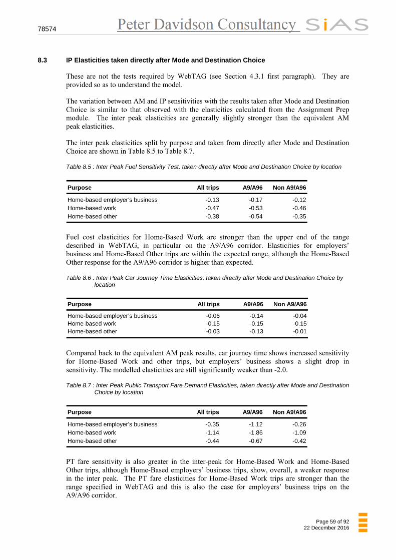
78574
Page 59 of 92 22 December 2016
8.3 IP Elasticities taken directly after Mode and Destination Choice
These are not the tests required by WebTAG (see Section 4.3.1 first paragraph). They are provided so as to understand the model.
The variation between AM and IP sensitivities with the results taken after Mode and Destination Choice is similar to that observed with the elasticities calculated from the Assignment Prep module. The inter peak elasticities are generally slightly stronger than the equivalent AM peak elasticities.
The inter peak elasticities split by purpose and taken from directly after Mode and Destination Choice are shown in Table 8.5 to Table 8.7.
Table 8.5 : Inter Peak Fuel Sensitivity Test, taken directly after Mode and Destination Choice by location
Purpose All trips A9/A96 Non A9/A96
Home-based employer’s business -0.13 -0.17 -0.12Home-based work -0.47 -0.53 -0.46Home-based other -0.38 -0.54 -0.35
Fuel cost elasticities for Home-Based Work are stronger than the upper end of the range described in WebTAG, in particular on the A9/A96 corridor. Elasticities for employers’ business and Home-Based Other trips are within the expected range, although the Home-Based Other response for the A9/A96 corridor is higher than expected.
Table 8.6 : Inter Peak Car Journey Time Elasticities, taken directly after Mode and Destination Choice by
location
Purpose All trips A9/A96 Non A9/A96
Home-based employer’s business -0.06 -0.14 -0.04Home-based work -0.15 -0.15 -0.15Home-based other -0.03 -0.13 -0.01
Compared back to the equivalent AM peak results, car journey time shows increased sensitivity for Home-Based Work and other trips, but employers’ business shows a slight drop in sensitivity. The modelled elasticities are still significantly weaker than -2.0.
Table 8.7 : Inter Peak Public Transport Fare Demand Elasticities, taken directly after Mode and Destination
Choice by location
Purpose All trips A9/A96 Non A9/A96
Home-based employer’s business -0.35 -1.12 -0.26Home-based work -1.14 -1.86 -1.09Home-based other -0.44 -0.67 -0.42
PT fare sensitivity is also greater in the inter-peak for Home-Based Work and Home-Based Other trips, although Home-Based employers’ business trips, show, overall, a weaker response in the inter peak. The PT fare elasticities for Home-Based Work trips are stronger than the range specified in WebTAG and this is also the case for employers’ business trips on the A9/A96 corridor.
78574
Page 60 of 92 22 December 2016
8.4 Summary of modelled elasticities
While WebTAG provides guidelines and reports on typical ranges of values, this study has estimated the coefficients from local Revealed Preference data with full sensitivity parameter estimation and good ‘t’ statistics. The results should be weighed up against the WebTAG evidence for a fair comparison, rather than simply referring to WebTAG ranges.
Looking at elasticities by purpose and time period most values fall within the broader ranges, although it should be noted that the modelled Home-Based Other elasticities are generally less sensitive than the Home-Based Work elasticities. Home-Based Other would normally be expected to be more sensitive than Home-Based Work on the basis that people making leisure journeys may be more willing to have a slower journey in return for cost savings so the model is either not behaving correctly or this is not reflected in the data or this study area is different or some combination of these. We suggest this is investigated at some convenient juncture.
Fuel sensitivities are mostly within WebTAG guidelines, with employers’ business trips being at the weaker end of the -0.1 to -0.4 range, although Home-Based Work trips, particularly on the A9/A96 corridor in the inter peak, are perhaps more sensitive than expected.
Car journey time elasticities are relatively weak when compared with fuel sensitivities, for example (though note that while the former are calculated on a trip basis, the latter use vehicle-kilometres), and are all within the WebTAG guidance.
PT fare elasticity is greater than the WebTAG guideline for Home-Based Work, particularly in the inter peak, but within the guidelines for all other purposes.
The PT fare elasticity is generally within the guidelines except for Home-Based Work, particularly within the inter peak.
The A9/A96 elasticities are generally higher than the non-A9/A96 elasticities, as would be expected.
The all-purpose averages we have obtained are within the recommended ranges. We have applied a series of more stringent tests, by splitting them by purpose. WebTAG does not suggest different values for different purposes except to suggest that fuel elasticities may be regarded as more plausible if they show values for Employers Business of around -0.1 and around -0.4 for Home-based other with Home-based work near the average, although it adds that there is little or no empirical evidence to support the variation by purpose. The model conforms to WebTAG apart from the Home-Based Other being less sensitive than the Home-Based Work, but the overall sensitivities are still within the guidelines.
All of the overall calculated elasticities based on the matrices at the Assignment Prep stage, i.e. before adding in external trips and applying the incremental matrices are within the WebTAG guidelines, however, care should be taken with forecasts for schemes where Home-based other trips experience more than the average journey time savings.
78574
Page 61 of 92 22 December 2016
9 FORECASTING PROCEDURES
9.1 Introduction
The function of the Base Year Demand Model is to:
Demonstrate and validate the model operation and procedures
Test the sensitivity of model parameters
Establish the incremental adjustment matrices
The forecasting process is designed to provide forecast matrices using an incremental procedure. The Base Year Demand Model structure is designed to operate in an iterative manner to deal with the supply/demand convergence issue.
The general application of the Demand Model for forecasting requires the following inputs:
Model parameters
Trip ends
Road and public transport cost matrices
Road and public transport networks
The requirements and sources of these inputs are described in Sections 9.4 to 9.7.
The treatment of goods vehicles, long distance trips and external trips in forecasting is dealt with in Sections 9.8, 9.9, and 9.10.
9.2 Overall Operation of the Demand Model
For a given forecast year and land-use scenario, the Trip End creation procedure is run to produce forecast trip productions and attractions. Analyses of the broad travel demand effects of the land-use planning and economic assumptions, excluding the impacts of travel costs, can be undertaken at this stage. The remaining sub-models operate in an iterative manner to produce final road traffic and public transport assignments.
The iterative balancing process is described in more detail in Appendix B. There are two main loops:
Inner Loops Iterate between the Mode Choice and Distribution Choice Models
External Loops Iterate between Assignment Models and the Mode and Destination Choice Models
The Inner Loops are the primary iterative process to achieve a converged state between the two main travel choices within the Demand Model - mode and distribution choice. It is necessary to undertake the Inner Loops before initiating the External Loop.
Note: The inner loops are not necessary for the singly constrained purposes, as the composite utilities do not change from loop to loop.
The Inner Loops can be run until a converged state is reached. This may vary with the forecast year and economic assumptions and between a Do-Minimum and Do-Something test. The model defaults to four such loops.

78574
Page 62 of 92 22 December 2016
The External Loop provides the link between the Assignment Models and the Demand Model. Infrastructure and pricing changes in a future year will change travel costs within the Assignment Models. The resultant converged state assigned travel costs are skimmed and supplied to the Distribution Choice using the same logsum composite utility calculations as for the Mode Choice Model. The sub-models are then run with the revised costs to complete the External Loop.
As standard, the Public Transport costs are set after one external loop of the Demand Model, however, if crowding effects (see PT Model report for a description of Crowding effects) are considered sufficient to cause large changes (such as to change the forecasts), it can be run on every external loop. The Road Assignment Model is run for each External Loop.
The External Loop should be run until a converged state is reached. The level of convergence achieved should be compared (using the current WebTAG guidance criteria) to determine if sufficient loops have been undertaken. This would vary with the forecast year and economic assumptions and between a Do-Minimum and Do-Something test. External Loop assignment matrices can be inspected between successive loops to determine whether to select to undertake further External Loops.
On each external loop of the demand model a process of trip damping takes place, which combines 50% of the current matrix, with 50% of that from the previous loop. This is the same in effect as the fixed step approach, which is included in DIADEM.
Gap analysis is undertaken on each External Demand Model Loop. This provides a measure of convergence of the demand model. It is not used as a stopping criteria, but the user can use it to assess if additional demand model loops need to be undertaken. The formulae for calculating the gap is given as:
100*'
' |
ijijij
ijijij
ij
TC
TTC
Gap
Where:
ijC is the generalised cost on the previous demand model loop
ijT are the trips on the previous demand model loop
'ijT are the trips on the current demand model loop
For models of this size gaps of less than 0.2 are deemed to be acceptable and below 0.1 is very well converged.

78574
Page 63 of 92 22 December 2016
9.3 The Incremental Forecasting Approach
The forecasting procedure for TMfS14 is designed to operate in a multiplicative incremental manner. Before using the TMfS14 model for forecasting, it had to be adjusted to produce trip matrices which reflected the observed or existing travel patterns.
This adjustment was done by generating a set of incremental matrices such that when they were combined with the synthesized matrices produced by the TMfS14 model, the resulting matrices matched the corresponding observed matrices. Thus, the combined synthesised and incremental matrices must adequately match the observed trips or travel patterns.
The cells in the incremental forecast matrices were generated in one of two ways:
Case 1 bf SBSF
Case 2
bf S
BSF *
Where B Base observed trips
bS Base modelled (synthesised) trips
fS Future modelled (synthesised) trips
F Future Trips
The following cases were defined when creating or applying the incremental matrices:
Case 1: Was used where B is zero or where we have high B and low Sb, defined as the case where B/Sb>2
Case 2: Was used in the following circumstances:
low B, high Sb
low B low Sb
high B high Sb
This allowed zero cells in the Base Year to be incremented using Case 1.
The terms in bracket formed the incremental matrices. The equations showed how they were applied in forecasting. Applying these models to estimate incremental changes from a well calibrated base situation removed the reliance on these factors in the forecasting process.
The Base Year matrices were accepted as the best representation of the existing travel pattern.
In this way, the Incremental Matrix remained constant for all applications and the forecast year synthesized trip matrices produced by a forecast run of the Demand Model were adjusted by the Incremental Matrix before assignment.
Once established these incremental matrices are applied to the Road and PT assignment matrices.

78574
Page 64 of 92 22 December 2016
9.4 Model Parameters
The need to calculate changes to some of the model parameters for a forecast run of the Demand Model is standard. The parameters for which forecast values are required which have been derived from WebTAG Databook, November 2014 are:
Generalised cost coefficients for Road assignment
Occupancy factors to convert from person to vehicle matrices
Values of time and vehicle operating costs
The mode specific constants calculated for the Base Year are specific to the Base Year distribution of single and multi-car owning households.
9.5 Road and Public Transport Cost Matrices
Generalised cost matrices by mode and at a zone level are required as inputs to start the Demand Model process. Normally, the cost matrices used are those from the Base Year model, but the user can choose to input forecast cost matrices to kick start a demand model run if they so wish.
The Base Year cost matrices by mode are also required for the calculation of the mode specific constants described previously.
Base or Reference Case Generalised Costs are used as the start point of variance case tests within the TMfS.
9.6 Road and Public Transport Networks
As input to a forecast model year run, there must be forecast year Reference Case and/or variant networks. These should be coded up as described by the Road and PT model development reports, by adding any additional schemes directly into the network models.
Consistency between the Road and PT models should be retained at all times.
9.7 Education Matrices
The Education Matrices were built from Census Travel to Work data and are included in the model as add in matrices at the post ‘inner loop’ stage of a model run.
The Education Matrices are growthed using planning data from TELMoS, the trip ends are forecast in a similar way to the other trip purposes and then the trips are distributed using a simple gravity model.
78574
Page 65 of 92 22 December 2016
9.8 Goods Vehicles
Goods vehicle trips are not subjected to the Demand Model process within the TMfS model. Forecast matrices are prepared using growth factors from the TELMoS commodity model.
The Base Year Goods PCU matrices at zonal level, are by hour (AM Peak, Inter Peak, and PM Peak) and by vehicle type, LGV and HGV. The forecasting process applied to these base matrices has the following three steps:
Calculate percentage growth on a cell by cell basis between TELMoS Base Year and forecast year commodity matrices (these cover internal goods vehicle movements within the TMfS modelled area)
Apply this percentage growth to the TMfS Base Year goods vehicle matrices
Apply National Road Traffic Forecasts (NRTF) growth to external movements
9.9 Long Distance Vehicle Matrices
Long Distance, but internal to Scotland, Employers Business and Other trips are forecast separately from the main demand model. There are two long distance models as follows:
Model 1: Long distance trips are added into the assignment matrices at the same stage as the Goods vehicle matrices (Long Distance trips are those defined as greater than 100km). The forecast procedure for long distance trips uses an elasticity model, based on assumed levels of growth in GDP over time. They are calculated in forecast mode for the full 12hr (07:00 – 19:00) time period and then factored to individual time periods. This process of factoring to the individual time periods uses the Base Year time period splits. Long Distance Trips were not treated differently in the base model. They are only treated differently in forecast mode. This is the default model for long distance trips.
Model 2: A long distance model including long distance mode and destination choice focussing on the A9/A96 corridor, was calibrated as part of the TMfS12 refresh. It can be invoked to replace Model 1 in the CUBE model code. It is documented in the TMfS12 documentation.
9.10 External Trips
External trips from England and Wales are dealt with as add-on external matrices. In forecast mode these are growthed using NRTF. The model user can, however, include whatever growth assumptions they wish.

78574
Page 66 of 92 22 December 2016
78574
Page 67 of 92 22 December 2016
10 CONCLUSIONS AND RECOMMENDATIONS
10.1 Conclusions
This document has described the development of the Base Year Demand Model for TMfS14, the Model’s sensitivity to a set of example tests and has discussed how the Model will be applied in forecast mode.
The model structure has been defined and implemented for the Base Year. The realism tests undertaken have demonstrated a good overall level of sensitivity. The principal travel purpose of the model, commute trips, has elasticities which fall well within the recommended sensitivity guidelines. Investigation of the elasticities in more detail has shown more variation some of which can be explained by the model structure adopted for this model and it is suggested that this is revisited when the model is next being considered for recalibration.
10.2 Recommendations
SIAS’s and PDC’s view is that the Demand Model is broadly fit for its intended purpose, i.e. being suitable for supporting the Outline Business Case for improvements on the Inverness to Aberdeen transport corridor and other such schemes.
The model as implemented in CUBE and described in its documentation contains some features where it is not clear that the structure implemented is as intended by its creators. It is recommended that the model architecture be re-structured more in-line with current practice at a suitable time in the model’s evolution.
While this report discusses how the model will be applied in forecast mode, it does not include consideration of actual applications of the model in forecast mode. Further experience of these applications gained over time will assist in understanding the sensitivity and performance of the Model.
All model applications should be preceded by an appropriate review of the robustness of the model in the area/corridor of interest.

78574
Page 68 of 92 22 December 2016
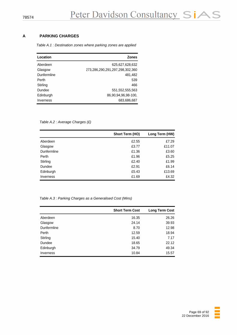
78574
Page 69 of 92 22 December 2016
A PARKING CHARGES
Table A.1 : Destination zones where parking zones are applied
Location Zones
Aberdeen 625,627,628,632Glasgow 273,286,290,291,297,298,302,360Dunfermline 481,482Perth 539Stirling 466Dundee 551,552,555,563Edinburgh 86,90,94,96,98-100,Inverness 683,686,687
Table A.2 : Average Charges (£)
Short Term (HO) Long Term (HW)
Aberdeen £2.55 £7.29Glasgow £3.77 £11.07Dunfermline £1.36 £3.60Perth £1.96 £5.25Stirling £2.40 £1.99Dundee £2.91 £6.14Edinburgh £5.43 £13.69Inverness £1.69 £4.32
Table A.3 : Parking Charges as a Generalised Cost (Mins)
Short Term Cost Long Term Cost
Aberdeen 16.35 26.26Glasgow 24.14 39.93Dunfermline 8.70 12.98Perth 12.59 18.94Stirling 15.40 7.17Dundee 18.65 22.12Edinburgh 34.79 49.34Inverness 10.84 15.57

78574
Page 70 of 92 22 December 2016
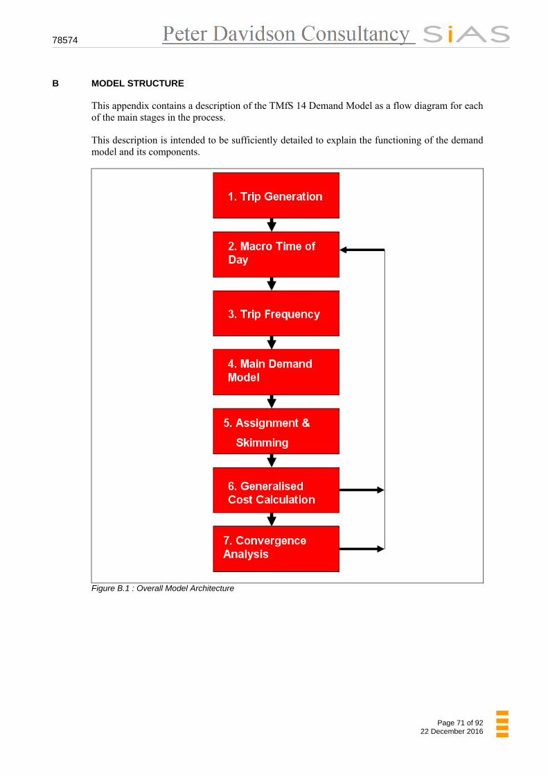
78574
Page 71 of 92 22 December 2016
B MODEL STRUCTURE
This appendix contains a description of the TMfS 14 Demand Model as a flow diagram for each of the main stages in the process.
This description is intended to be sufficiently detailed to explain the functioning of the demand model and its components.
Figure B.1 : Overall Model Architecture
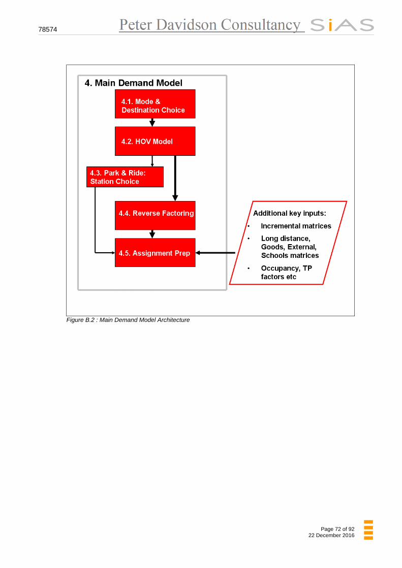
78574
Page 72 of 92 22 December 2016
Figure B.2 : Main Demand Model Architecture
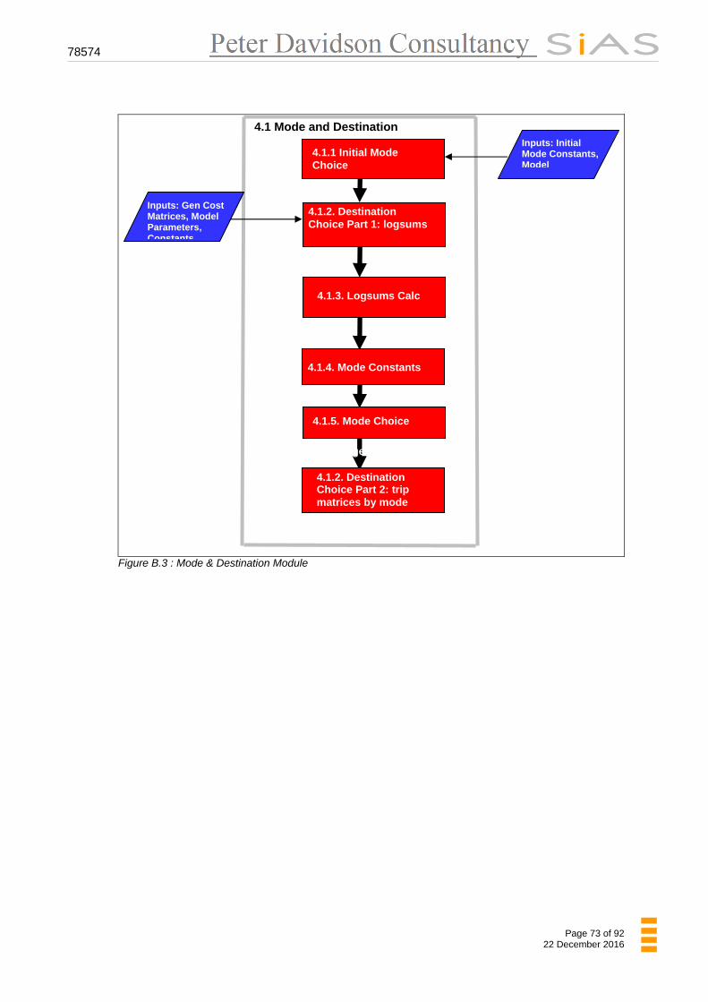
78574
Page 73 of 92 22 December 2016
Figure B.3 : Mode & Destination Module
4.1.1 Initial Mode Choice
7. Convergence Analysis
8. Post Run Analysis
4.1.3. Logsums Calc
4.1.5. Mode Choice
4.1.2. Destination Choice Part 1: logsums
4.1.4. Mode Constants
4.1 Mode and Destination Inputs: Initial Mode Constants, Model
Inputs: Gen Cost Matrices, Model Parameters, Constants
4.1.2. Destination Choice Part 2: trip matrices by mode
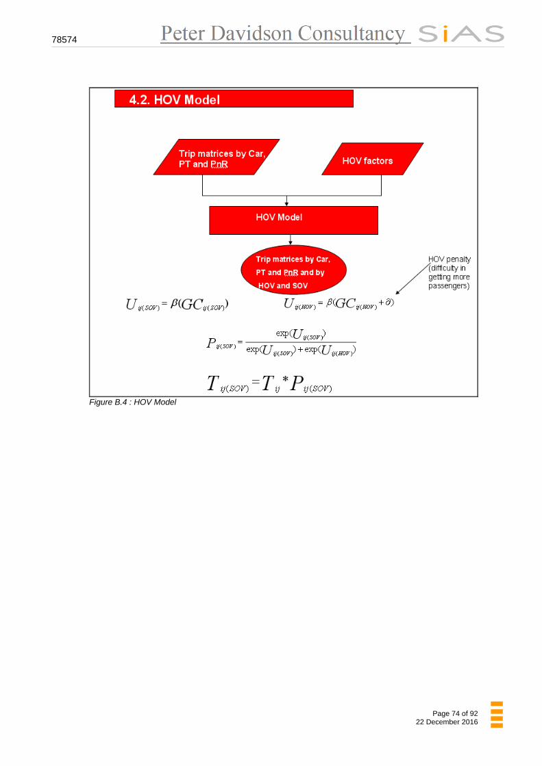
78574
Page 74 of 92 22 December 2016
Figure B.4 : HOV Model
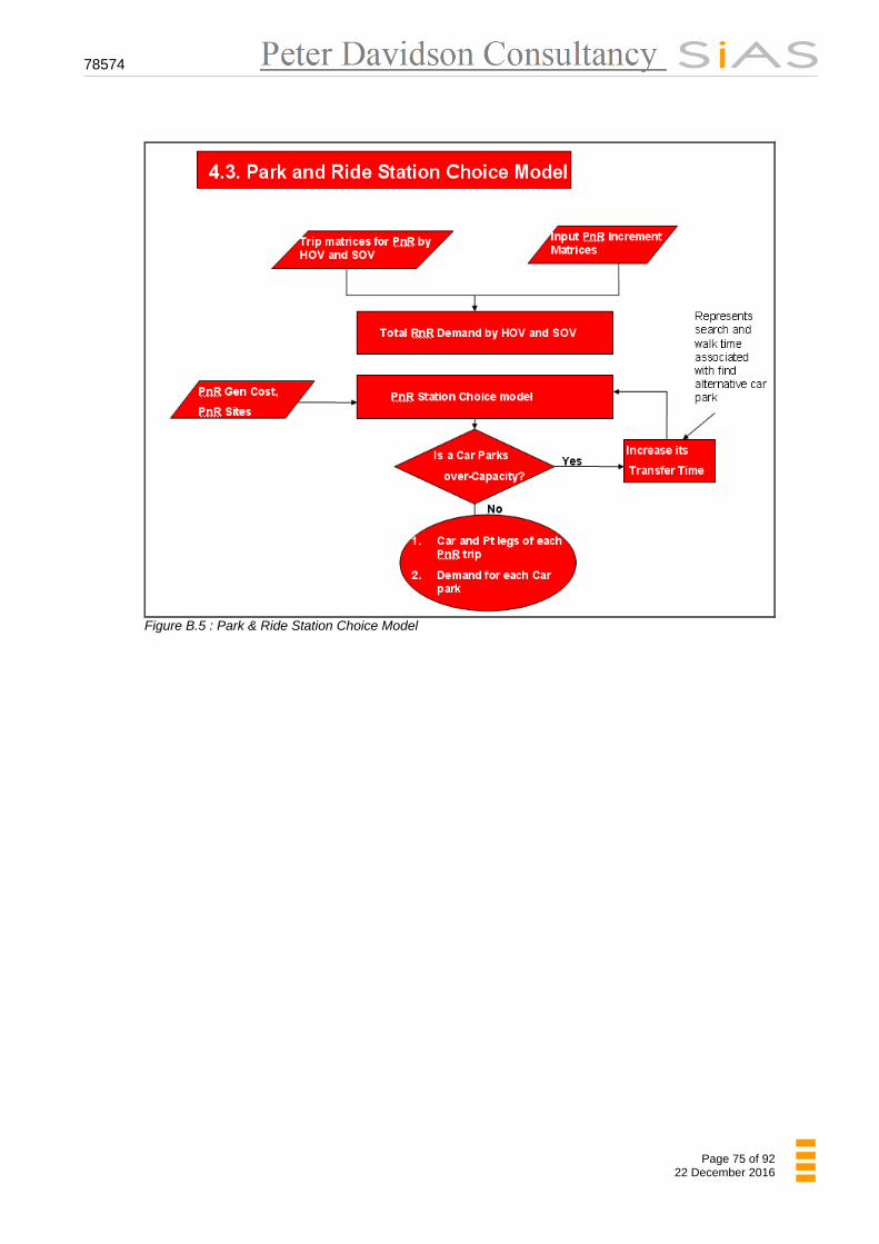
78574
Page 75 of 92 22 December 2016
Figure B.5 : Park & Ride Station Choice Model
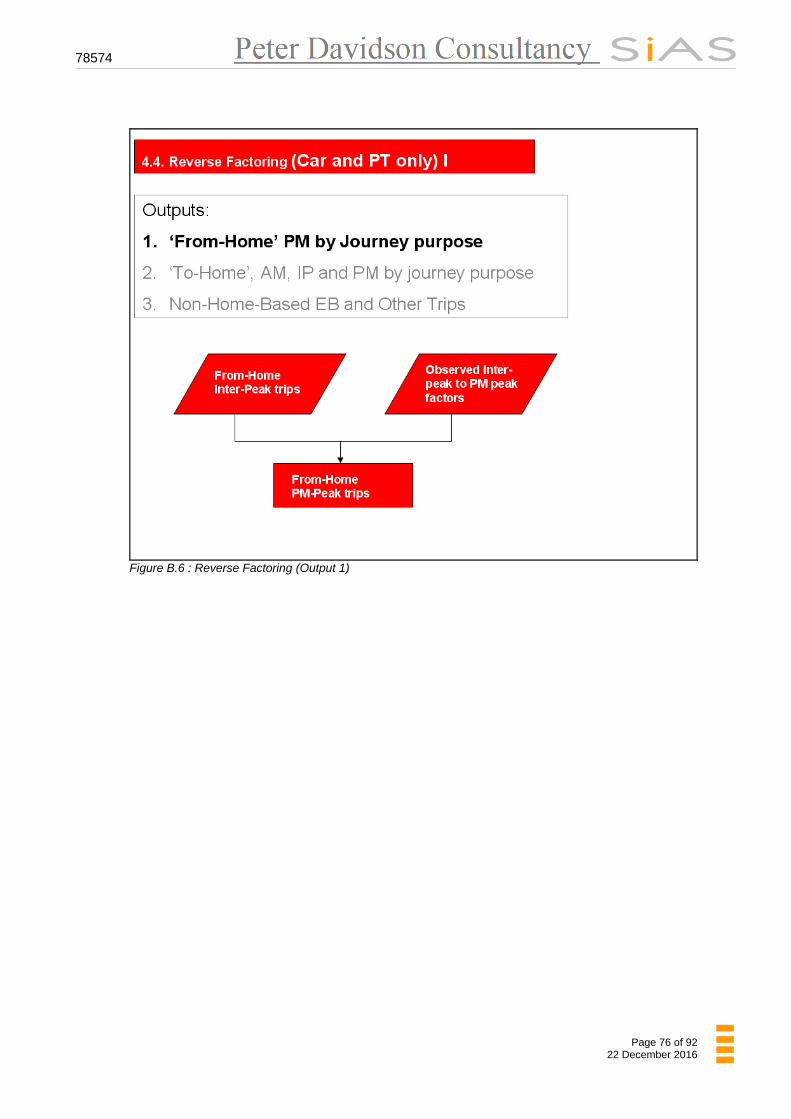
78574
Page 76 of 92 22 December 2016
Figure B.6 : Reverse Factoring (Output 1)
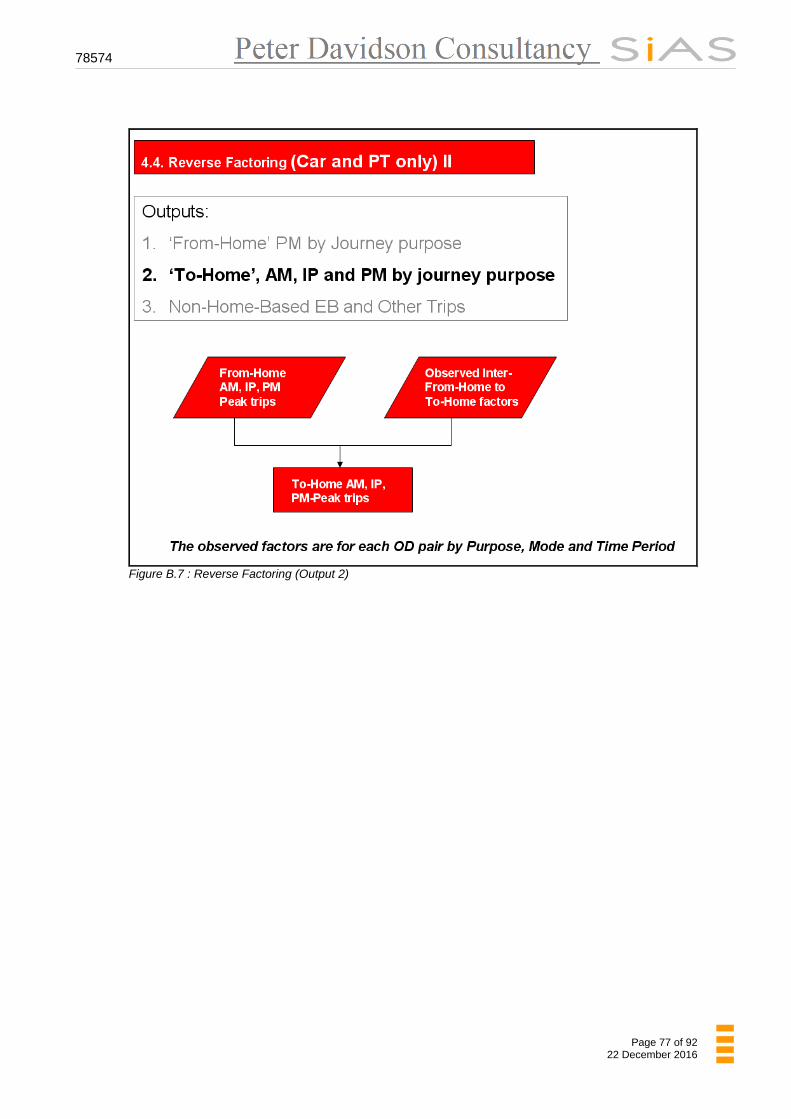
78574
Page 77 of 92 22 December 2016
Figure B.7 : Reverse Factoring (Output 2)
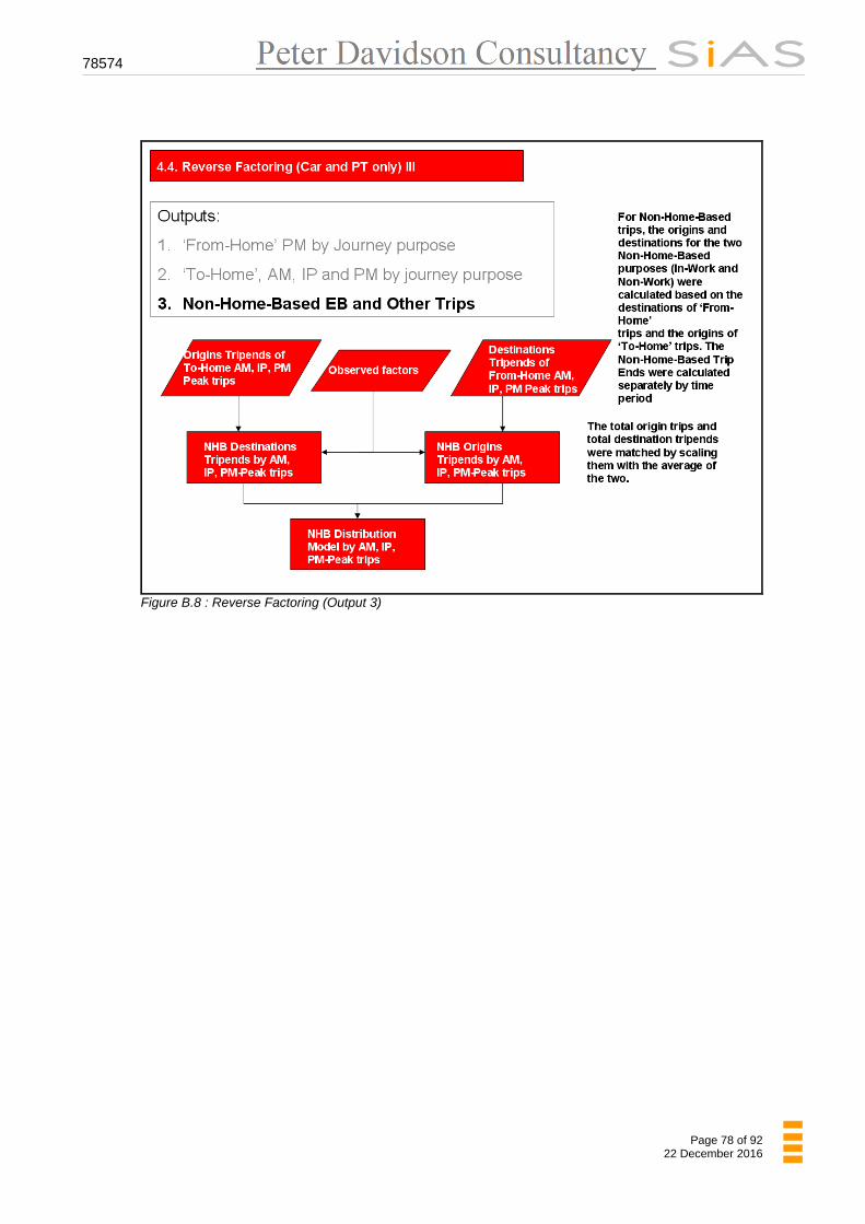
78574
Page 78 of 92 22 December 2016
Figure B.8 : Reverse Factoring (Output 3)
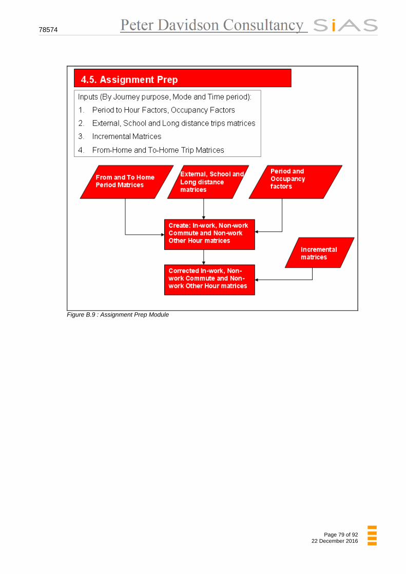
78574
Page 79 of 92 22 December 2016
Figure B.9 : Assignment Prep Module

78574
Page 80 of 92 22 December 2016
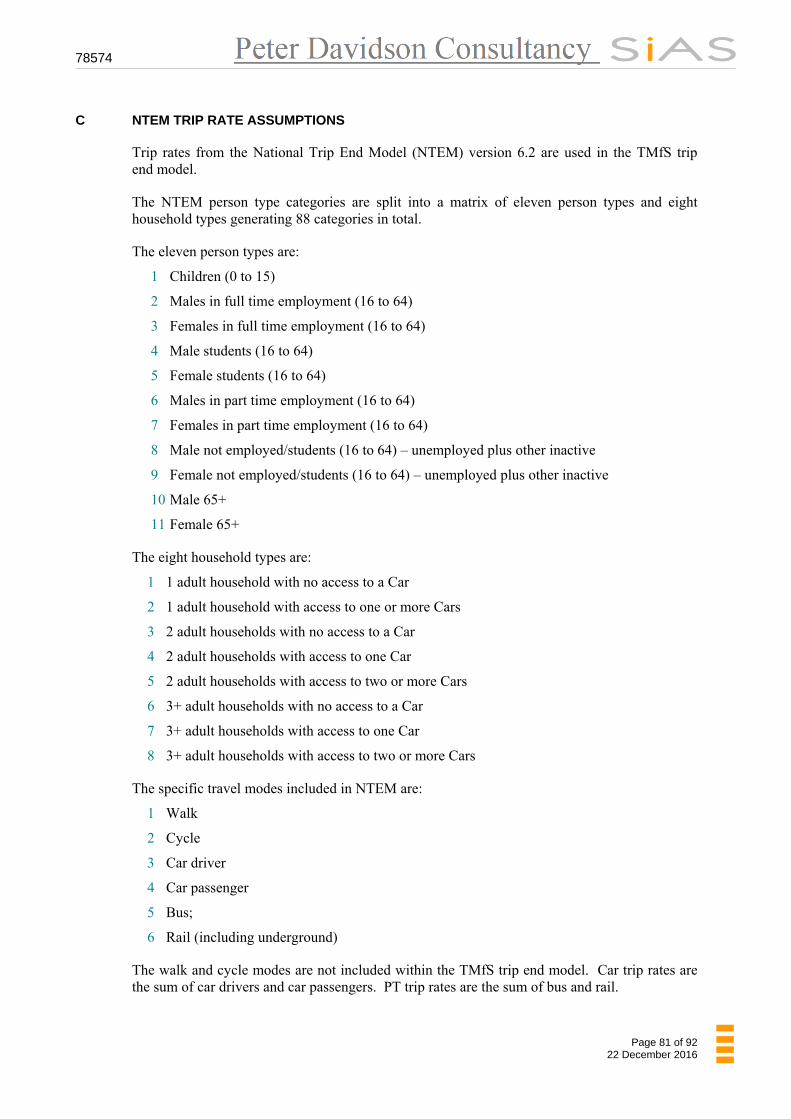
78574
Page 81 of 92 22 December 2016
C NTEM TRIP RATE ASSUMPTIONS
Trip rates from the National Trip End Model (NTEM) version 6.2 are used in the TMfS trip end model.
The NTEM person type categories are split into a matrix of eleven person types and eight household types generating 88 categories in total.
The eleven person types are:
1 Children (0 to 15)
2 Males in full time employment (16 to 64)
3 Females in full time employment (16 to 64)
4 Male students (16 to 64)
5 Female students (16 to 64)
6 Males in part time employment (16 to 64)
7 Females in part time employment (16 to 64)
8 Male not employed/students (16 to 64) – unemployed plus other inactive
9 Female not employed/students (16 to 64) – unemployed plus other inactive
10 Male 65+
11 Female 65+
The eight household types are:
1 1 adult household with no access to a Car
2 1 adult household with access to one or more Cars
3 2 adult households with no access to a Car
4 2 adult households with access to one Car
5 2 adult households with access to two or more Cars
6 3+ adult households with no access to a Car
7 3+ adult households with access to one Car
8 3+ adult households with access to two or more Cars
The specific travel modes included in NTEM are:
1 Walk
2 Cycle
3 Car driver
4 Car passenger
5 Bus;
6 Rail (including underground)
The walk and cycle modes are not included within the TMfS trip end model. Car trip rates are the sum of car drivers and car passengers. PT trip rates are the sum of bus and rail.

78574
Page 82 of 92 22 December 2016
Production trip rates for these 88 categories are obtained from the NTEM databases. The IBETAhsr table is used to provide the weekly trip rates by purpose, traveller type and area type. The IRhomdhsr table is used to split these trip rates by time period and mode.
For TMfS12, Area Type 5 (Urban Medium) trip rates are applied as this was considered to be the most appropriate assumption or average set of trip rates for the TMfS coverage area. For TMfS12A the trip end model has been improved to use all area types so that, for example, modelled trip rates in cities will be different to rural locations.
The trip rates are constant over all modelled years.

78574
Page 83 of 92 22 December 2016
D PARK & RIDE CALIBRATION
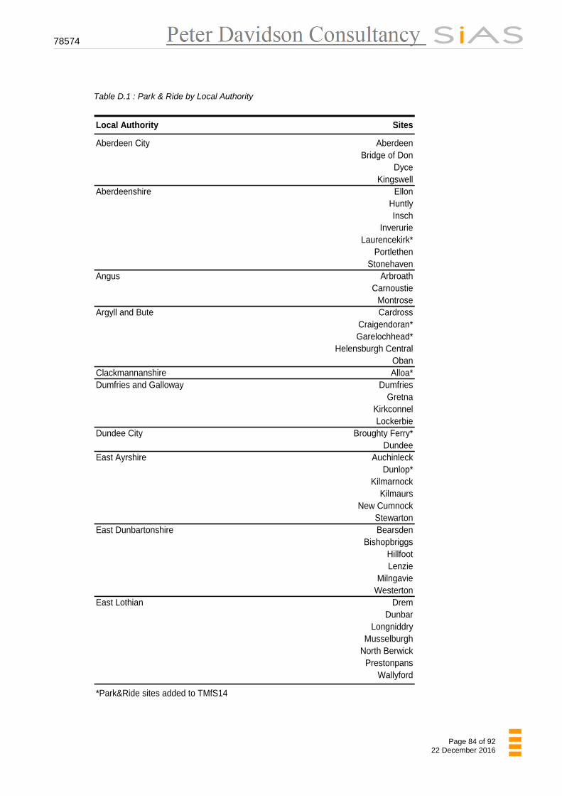
78574
Page 84 of 92 22 December 2016
Table D.1 : Park & Ride by Local Authority
Local Authority Sites
Aberdeen City AberdeenBridge of Don
DyceKingswell
Aberdeenshire EllonHuntlyInsch
InverurieLaurencekirk*
PortlethenStonehaven
Angus ArbroathCarnoustie
MontroseArgyll and Bute Cardross
Craigendoran*Garelochhead*
Helensburgh CentralOban
Clackmannanshire Alloa*Dumfries and Galloway Dumfries
GretnaKirkconnelLockerbie
Dundee City Broughty Ferry*Dundee
East Ayrshire AuchinleckDunlop*
KilmarnockKilmaurs
New CumnockStewarton
East Dunbartonshire BearsdenBishopbriggs
HillfootLenzie
MilngavieWesterton
East Lothian DremDunbar
LongniddryMusselburgh
North BerwickPrestonpans
Wallyford
*Park&Ride sites added to TMfS14
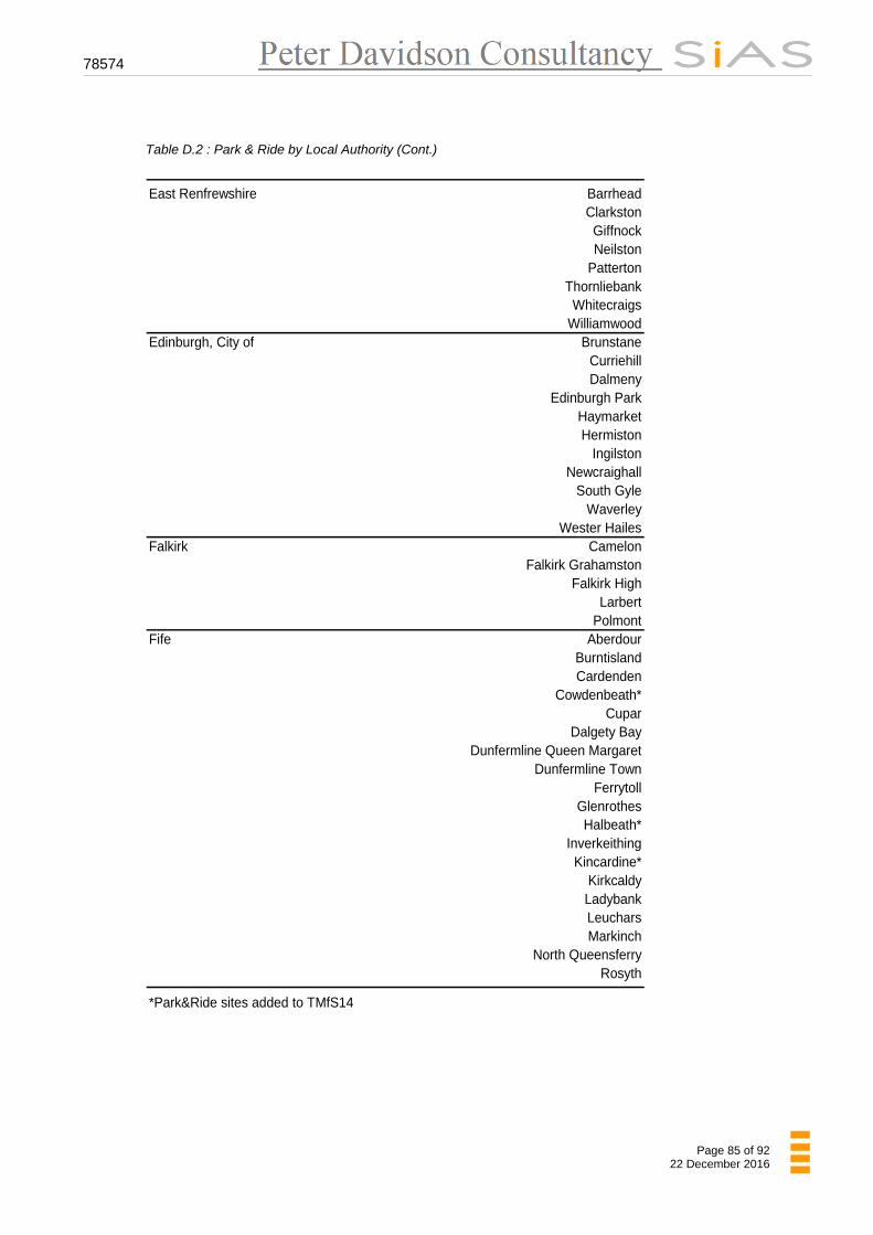
78574
Page 85 of 92 22 December 2016
Table D.2 : Park & Ride by Local Authority (Cont.)
East Renfrewshire Barrhead
ClarkstonGiffnockNeilston
PattertonThornliebankWhitecraigs
WilliamwoodEdinburgh, City of Brunstane
CurriehillDalmeny
Edinburgh ParkHaymarketHermiston
IngilstonNewcraighall
South GyleWaverley
Wester HailesFalkirk Camelon
Falkirk GrahamstonFalkirk High
LarbertPolmont
Fife AberdourBurntislandCardenden
Cowdenbeath*Cupar
Dalgety BayDunfermline Queen Margaret
Dunfermline TownFerrytoll
GlenrothesHalbeath*
InverkeithingKincardine*
KirkcaldyLadybankLeucharsMarkinch
North QueensferryRosyth
*Park&Ride sites added to TMfS14

78574
Page 86 of 92 22 December 2016
Table D.3 : Park & Ride by Local Authority (Cont.)
Glasgow City Anniesland
BellgroveBridge Street Subway*
BridgetonCardonald
CathcartCharing Cross
DrumchapelEasterhouse
GarrowhillGlasgow Central
Glasgow Queen StHigh Street Glasgow
HyndlandJordanhill*
KelvinbridgeKelvinbridge SubwayKinross (Govanhill)*
MuirendPartick
ScotstounhillShettleston
Shield RdShieldmuir*Silverburn*
Highland AviemoreFort William
InvernessKingussie
Kirkhill*Kyle of Lochalsh
NairnStromeferry
Inverclyde BranchtonFort Matilda
GourockGreenock Central
Greenock WestInverkip*
Port GlasgowWemyss Bay
Midlothian Sheriffhall*Straiton*
Moray ElginForres
Keith
*Park&Ride sites added to TMfS14

78574
Page 87 of 92 22 December 2016
Table D.4 : Park & Ride by Local Authority (Cont.)
North Ayrshire Ardrossan South BeachDalry
Fairlie*Glengarnock
IrvineKilwinning
Largs*Saltcoats
West Kilbride*North Lanarkshire Airbles
AirdrieBargeddie
BellshillBlairhill
Caldercruix*Carfin*
ClelandCoatbridge Central*
Coatbridge SunnysideCoatdyke
CroyCumbernauldDrumgelloch
GartcoshGreenfaulds
Harthill*Hartwood*
HolytownKirkwood*
MotherwellNewhouse*
ShottsSteppsWhiffletWishaw
Perth and Kinross Broxden PerthDunkeld & Birnam
GleneaglesKinross (Perthshire)
PerthPitlochryRannoch
Scone*
*Park&Ride sites added to TMfS14
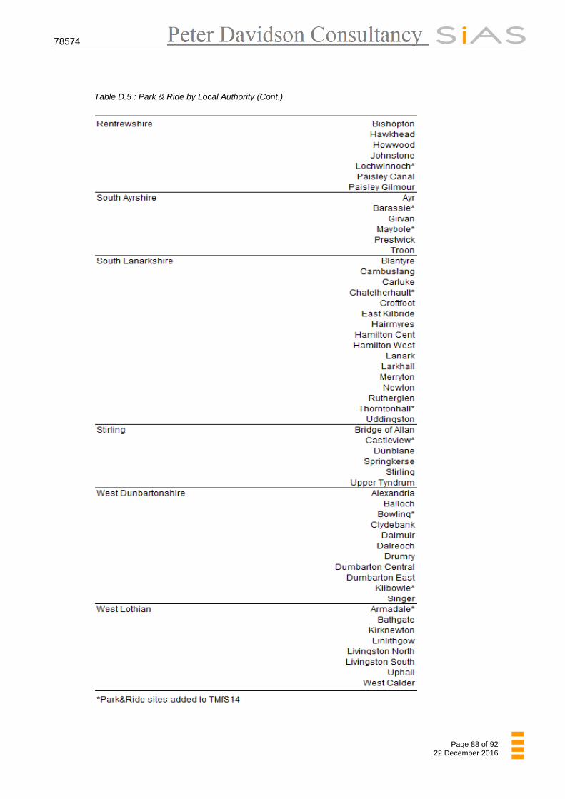
78574
Page 88 of 92 22 December 2016
Table D.5 : Park & Ride by Local Authority (Cont.)
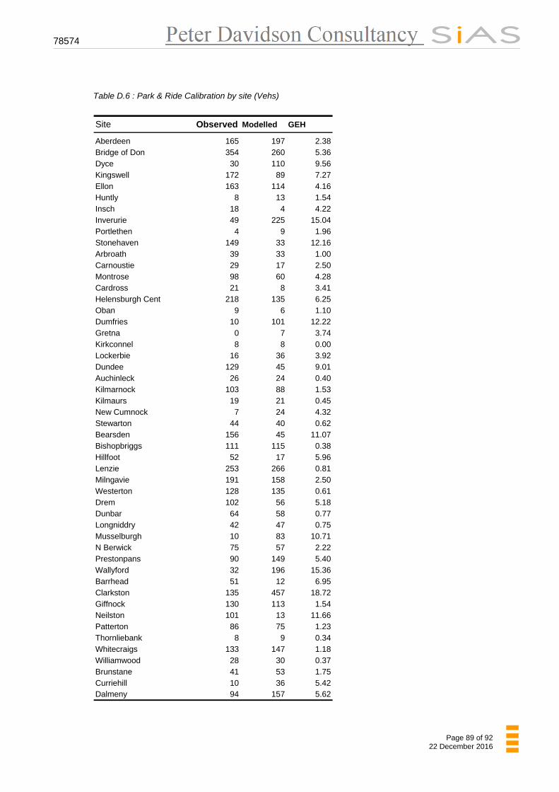
78574
Page 89 of 92 22 December 2016
Table D.6 : Park & Ride Calibration by site (Vehs)
Site Observed Modelled GEH
Aberdeen 165 197 2.38Bridge of Don 354 260 5.36Dyce 30 110 9.56Kingswell 172 89 7.27Ellon 163 114 4.16Huntly 8 13 1.54Insch 18 4 4.22Inverurie 49 225 15.04Portlethen 4 9 1.96Stonehaven 149 33 12.16Arbroath 39 33 1.00Carnoustie 29 17 2.50Montrose 98 60 4.28Cardross 21 8 3.41Helensburgh Cent 218 135 6.25Oban 9 6 1.10Dumfries 10 101 12.22Gretna 0 7 3.74Kirkconnel 8 8 0.00Lockerbie 16 36 3.92Dundee 129 45 9.01Auchinleck 26 24 0.40Kilmarnock 103 88 1.53Kilmaurs 19 21 0.45New Cumnock 7 24 4.32Stewarton 44 40 0.62Bearsden 156 45 11.07Bishopbriggs 111 115 0.38Hillfoot 52 17 5.96Lenzie 253 266 0.81Milngavie 191 158 2.50Westerton 128 135 0.61Drem 102 56 5.18Dunbar 64 58 0.77Longniddry 42 47 0.75Musselburgh 10 83 10.71N Berwick 75 57 2.22Prestonpans 90 149 5.40Wallyford 32 196 15.36Barrhead 51 12 6.95Clarkston 135 457 18.72Giffnock 130 113 1.54Neilston 101 13 11.66Patterton 86 75 1.23Thornliebank 8 9 0.34Whitecraigs 133 147 1.18Williamwood 28 30 0.37Brunstane 41 53 1.75Curriehill 10 36 5.42Dalmeny 94 157 5.62
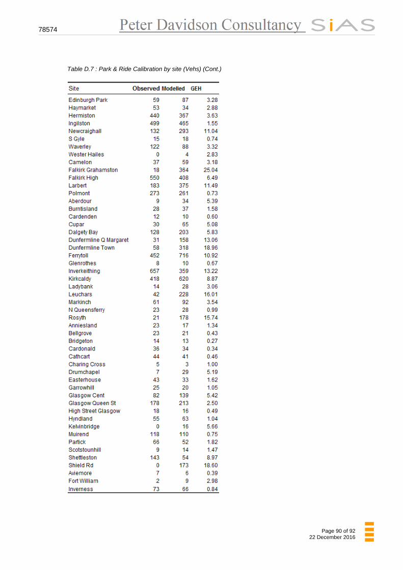
78574
Page 90 of 92 22 December 2016
Table D.7 : Park & Ride Calibration by site (Vehs) (Cont.)
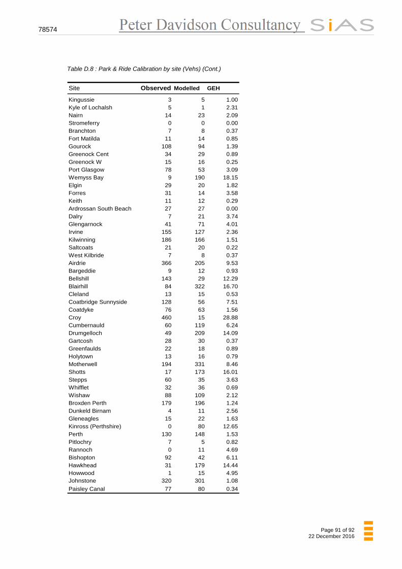
78574
Page 91 of 92 22 December 2016
Table D.8 : Park & Ride Calibration by site (Vehs) (Cont.)
Site Observed Modelled GEH
Kingussie 3 5 1.00Kyle of Lochalsh 5 1 2.31Nairn 14 23 2.09Stromeferry 0 0 0.00Branchton 7 8 0.37Fort Matilda 11 14 0.85Gourock 108 94 1.39Greenock Cent 34 29 0.89Greenock W 15 16 0.25Port Glasgow 78 53 3.09Wemyss Bay 9 190 18.15Elgin 29 20 1.82Forres 31 14 3.58Keith 11 12 0.29Ardrossan South Beach 27 27 0.00Dalry 7 21 3.74Glengarnock 41 71 4.01Irvine 155 127 2.36Kilwinning 186 166 1.51Saltcoats 21 20 0.22West Kilbride 7 8 0.37Airdrie 366 205 9.53Bargeddie 9 12 0.93Bellshill 143 29 12.29Blairhill 84 322 16.70Cleland 13 15 0.53Coatbridge Sunnyside 128 56 7.51Coatdyke 76 63 1.56Croy 460 15 28.88Cumbernauld 60 119 6.24Drumgelloch 49 209 14.09Gartcosh 28 30 0.37Greenfaulds 22 18 0.89Holytown 13 16 0.79Motherwell 194 331 8.46Shotts 17 173 16.01Stepps 60 35 3.63Whifflet 32 36 0.69Wishaw 88 109 2.12Broxden Perth 179 196 1.24Dunkeld Birnam 4 11 2.56Gleneagles 15 22 1.63Kinross (Perthshire) 0 80 12.65Perth 130 148 1.53Pitlochry 7 5 0.82Rannoch 0 11 4.69Bishopton 92 42 6.11Hawkhead 31 179 14.44Howwood 1 15 4.95Johnstone 320 301 1.08
Paisley Canal 77 80 0.34
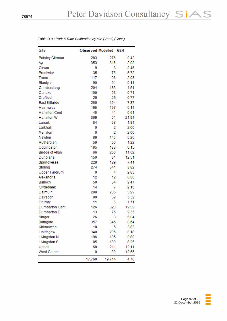
78574
Page 92 of 92 22 December 2016
Table D.9 : Park & Ride Calibration by site (Vehs) (Cont.)