Super-Regenerative Receiver

Ultra low-power RF Transceiver for high input power & low-data rate applications

ECEN 665 TAMU AMSC

Thanks to this material to Felix Fernandez

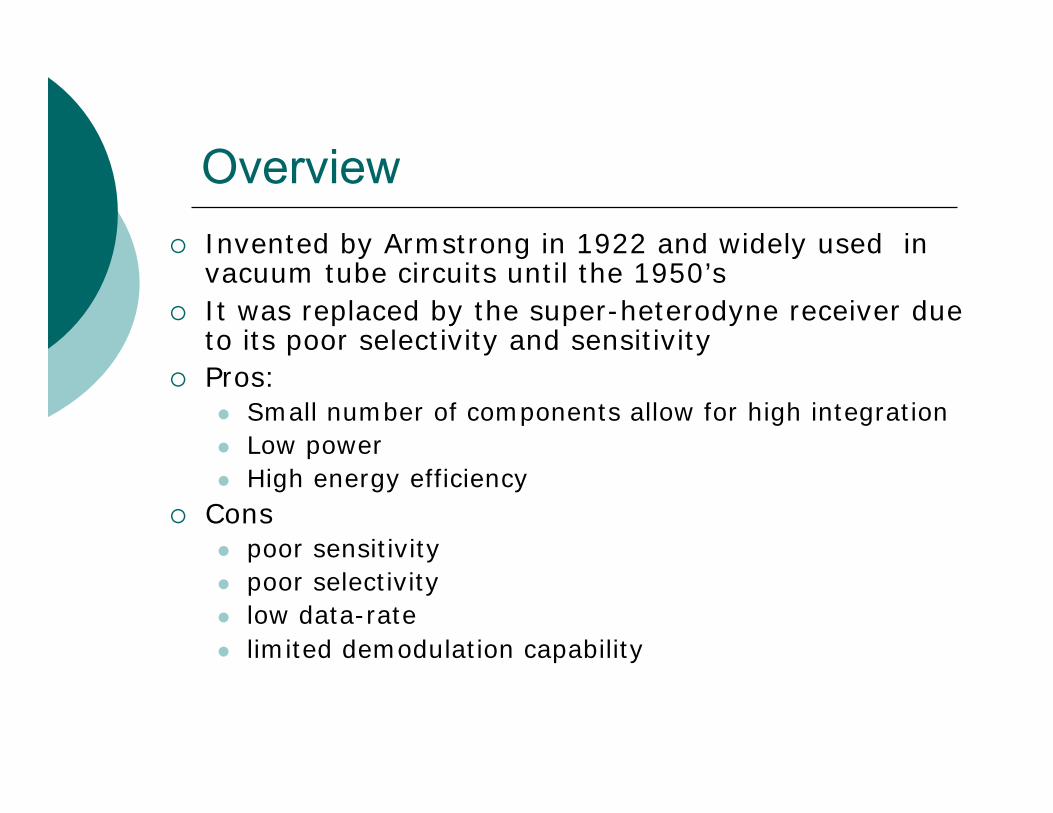
OverviewInvented by Armstrong in 1922 and widely used in vacuum tube circuits until the 1950’s It was replaced by the super-heterodyne receiver due to its poor selectivity and sensitivityPros:

Small number of components allow for high integrationLow powerHigh energy efficiency

Cons poor sensitivity poor selectivity low data-ratelimited demodulation capability

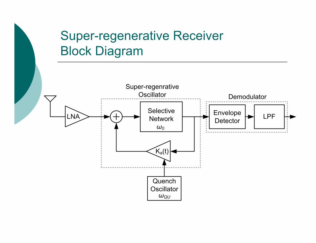
Super-regenerative Receiver Block Diagram

SelectiveNetwork

Ka(t)

QuenchOscillator

LNA EnvelopeDetector LPF

DemodulatorSuper-regenrative

Oscillator

ω0

ωQU

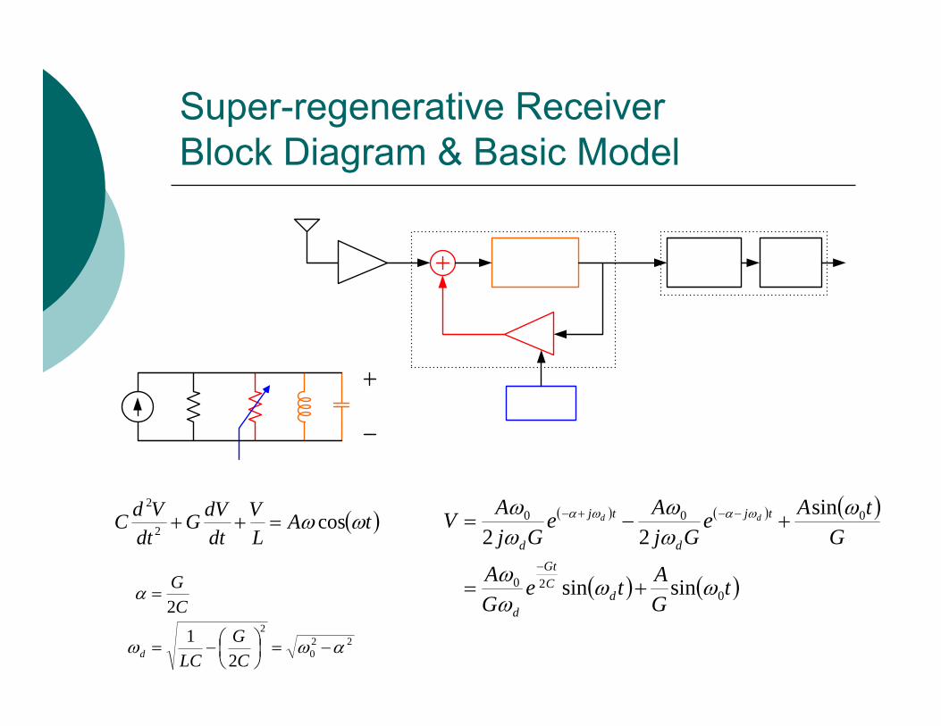
Super-regenerative Receiver Block Diagram & Basic Model

( )tALV

dtdVG

dtVdC ωω cos2

2

=++ ( ) ( ) ( )

( ) ( )tGAte

GA

GtAe

GjAe

GjAV

dCGt

d

tj

d

tj

d

dd

020

000

sinsin

sin22

ωωωω

ωωω

ωω ωαωα

+=

+−=

−

−−+−

220

2

21

2

αωω

α

−=⎟⎠⎞

⎜⎝⎛−=

=

CG

LC

CG

d

WWII –German Air Interception(first generation SRR, circa 1940)

Operation Fundamentals

Ga(t) = G0

Ga(t) = 0 [Ga(t) is a negative conductance]

Ga(t) >> G0

Pole-Zero Map

Real Axis

Imag

inar

y Ax

is

-8000 -6000 -4000 -2000 0 2000 4000-8

-6

-4

-2

0

2

4

6

8x 10

4

Bode Diagram

Frequency (rad/sec)10

410

510

6-40

-20

0

20

40

60

80

100

120

140From: Input Point To: Output Point

Mag

nitu

de (d

B)

stab

le o

per

atio

n

close

to u

nst

able

(hig

h Q

)

unst

able

oper

ation

( )v(t)i(t)

tG =

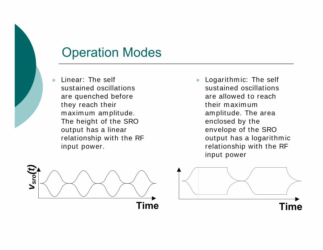
Operation Modes

Linear: The self sustained oscillations are quenched before they reach their maximum amplitude. The height of the SRO output has a linear relationship with the RF input power.

Logarithmic: The self sustained oscillations are allowed to reach their maximum amplitude. The area enclosed by the envelope of the SRO output has a logarithmic relationship with the RF input power

v sro

(t)

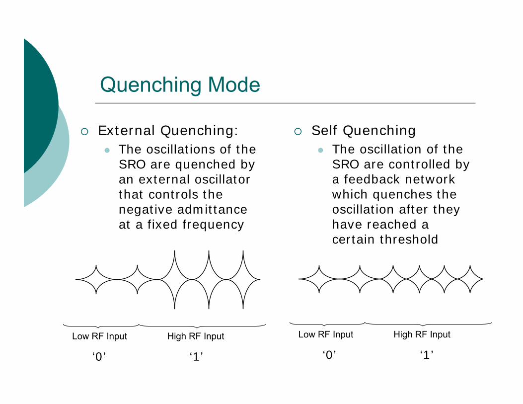
Quenching Mode

External Quenching:The oscillations of the SRO are quenched by an external oscillator that controls the negative admittance at a fixed frequency

Self QuenchingThe oscillation of the SRO are controlled by a feedback network which quenches the oscillation after they have reached a certain threshold

Low RF Input High RF Input Low RF Input High RF Input

‘0’ ‘1’ ‘0’ ‘1’

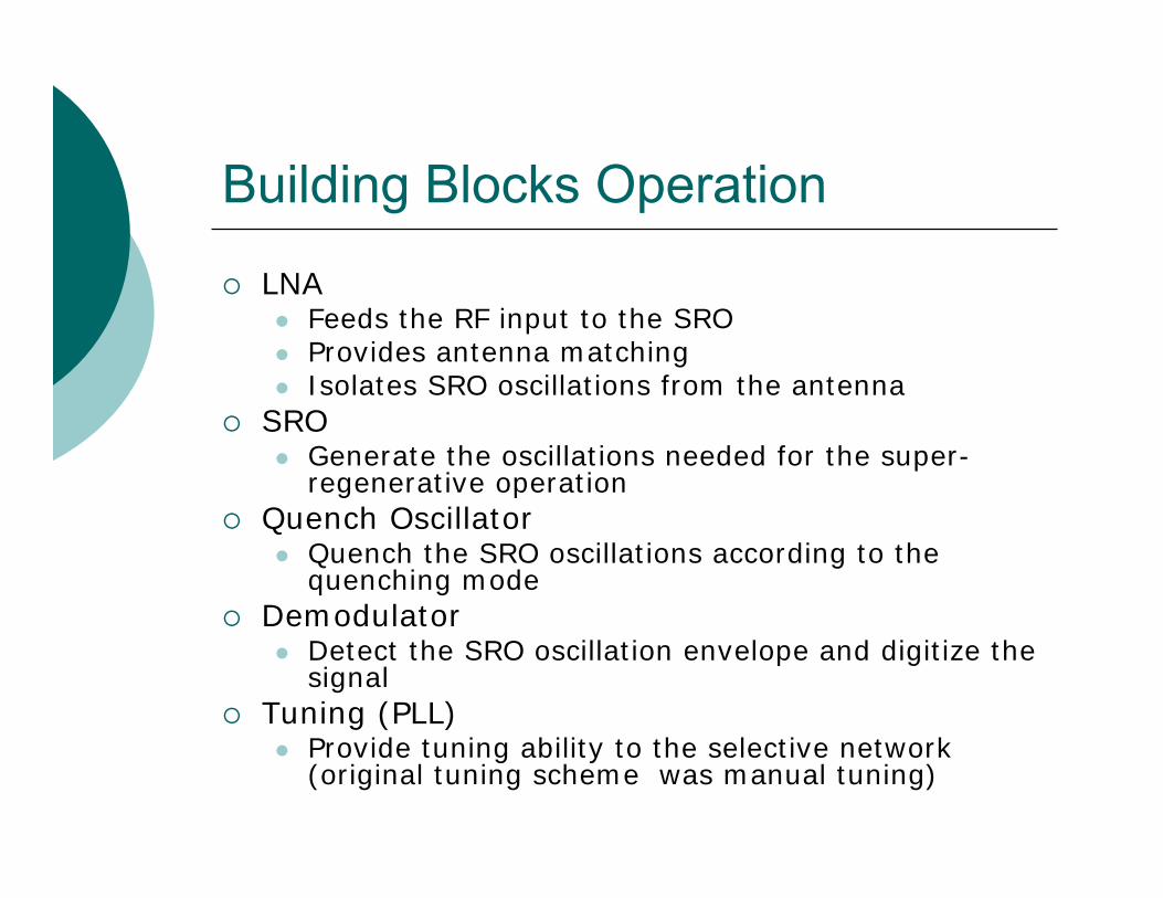
Building Blocks Operation

LNAFeeds the RF input to the SROProvides antenna matchingIsolates SRO oscillations from the antenna

SROGenerate the oscillations needed for the super-regenerative operation

Quench OscillatorQuench the SRO oscillations according to the quenching mode

DemodulatorDetect the SRO oscillation envelope and digitize the signal

Tuning (PLL)Provide tuning ability to the selective network (original tuning scheme was manual tuning)

Super Regenerative SystemDesign Equations

( )

( )( )

( )( )∫

=

∫=

∫=

−

−

t

t

bt

bt

dtt

dtt

dtt

s

ets

etp

eK

00

0

00

ζω

ζω

ζω

Super regenerative gain

Output pulse shape

Sensitivity function

Frequency response is given by the Fourier transform of the RF envelope and the sensitivity function.

ttQ

O

e )(2ω

−

ζ(t)

ζAVG

ta tbt

ta tbt

s(t)1 p(t)

i(t)

G0 -Ga(t) L Ci(t)

{ })()( tstiF

Selective Network Design Equations

( ) 2000

200

0 22

ωωζωζ

++=

sssKsG

( ) ( )( ) aKsGsGsH

+=

1

±: depends on the quench control signal

( ) ( )( )tKKt a00 1−= ζζ

( ))(2

1t

tQζ

=

K0: maximum amplificationKa(t): variable gain controlled by quench signalζ0: quiescent damping factorζAVG: damping factor average value

( )attaa tKK ==*

( ) ( ) 20

*000

200

0 122

ωωζωζ

+±+=

sKKssKsH

a

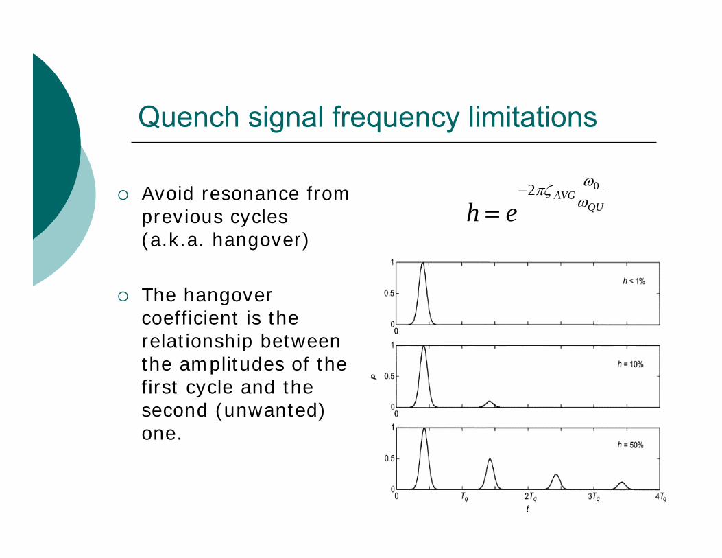
Quench signal frequency limitations

Avoid resonance from previous cycles (a.k.a. hangover)

The hangover coefficient is the relationship between the amplitudes of the first cycle and the second (unwanted) one.

QUAVG

eh ωωπζ 02−

=

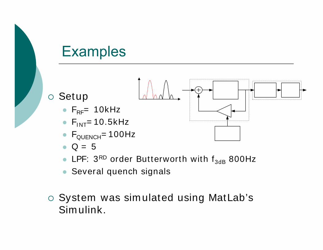
Examples

SetupFRF= 10kHzFINT=10.5kHzFQUENCH=100HzQ = 5LPF: 3RD order Butterworth with f3dB 800HzSeveral quench signals

System was simulated using MatLab’sSimulink.

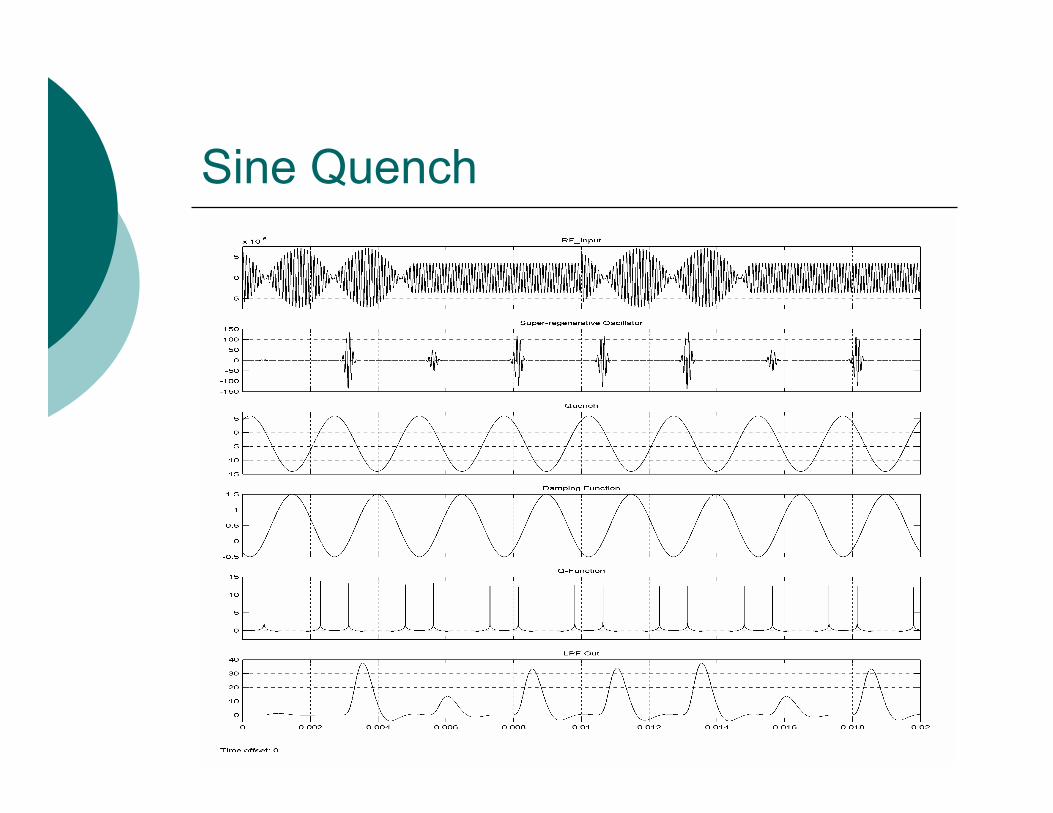
Sine Quench

Sawtooth Quench

-0.05 -0.04 -0.03 -0.02 -0.01 0 0.01 0.02 0.03 0.04 0.05-50

-45

-40

-35

-30

-25

-20

-15

-10

-5

0

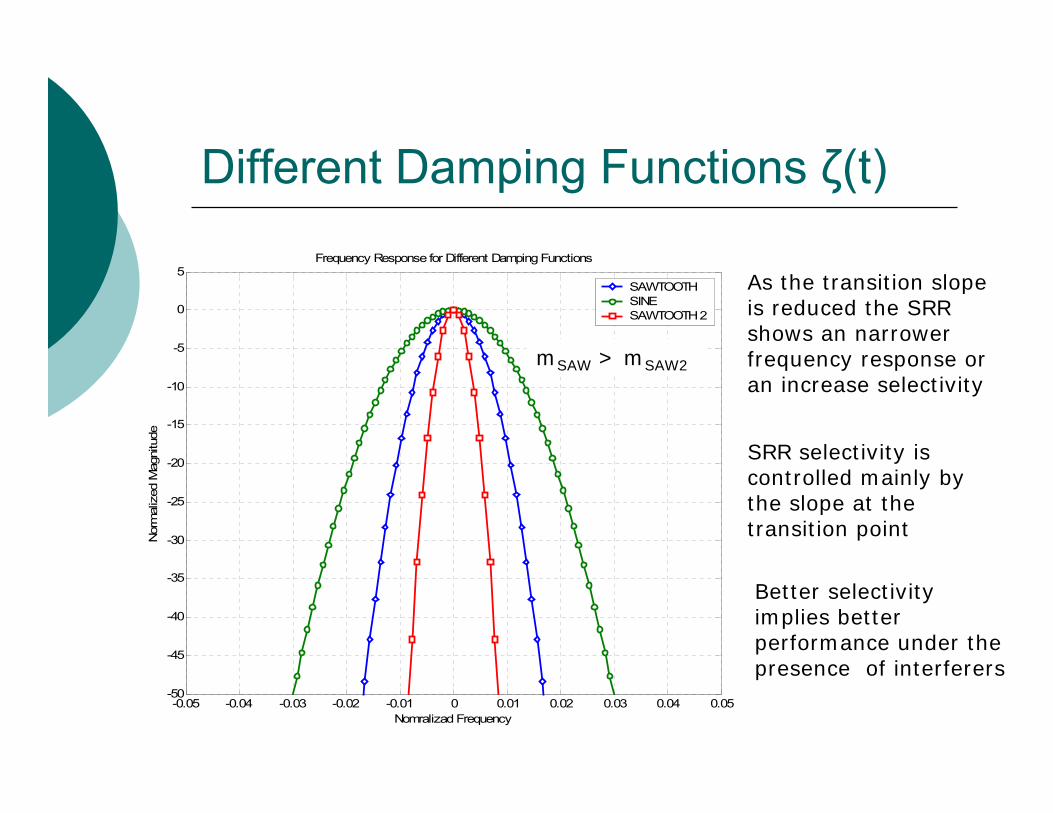
5Frequency Response for Different Damping Functions

Nomralizad Frequency

Nor

mal

ized

Mag

nitu

de

SAWTOOTHSINESAWTOOTH 2

Different Damping Functions ζ(t)

As the transition slope is reduced the SRR shows an narrower frequency response or an increase selectivity

SRR selectivity is controlled mainly by the slope at the transition point

Better selectivity implies better performance under the presence of interferers

mSAW > mSAW2

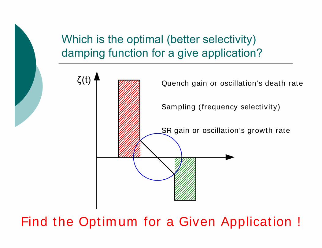
Which is the optimal (better selectivity) damping function for a give application?

Quench gain or oscillation’s death rate

Sampling (frequency selectivity)

SR gain or oscillation’s growth rate

Find the Optimum for a Given Application !

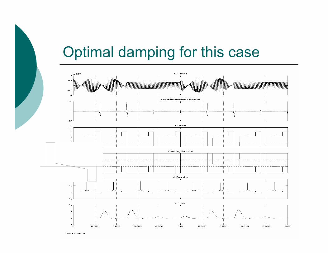
Optimal damping for this case

Modern Applications

SRR today:Ultra low power communication require minimum energy consumption during the RF communication

Application fields: short-distance data-exchange wireless link with medium data-rate, such as sensor network, home automation, robotics, computer peripherals, or biomedicine.

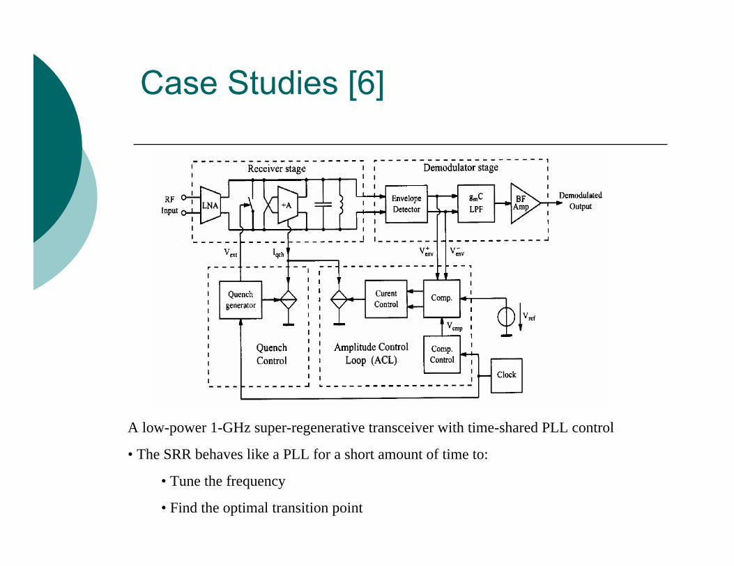
Case Studies [6]

A low-power 1-GHz super-regenerative transceiver with time-shared PLL control

• The SRR behaves like a PLL for a short amount of time to:

• Tune the frequency

• Find the optimal transition point

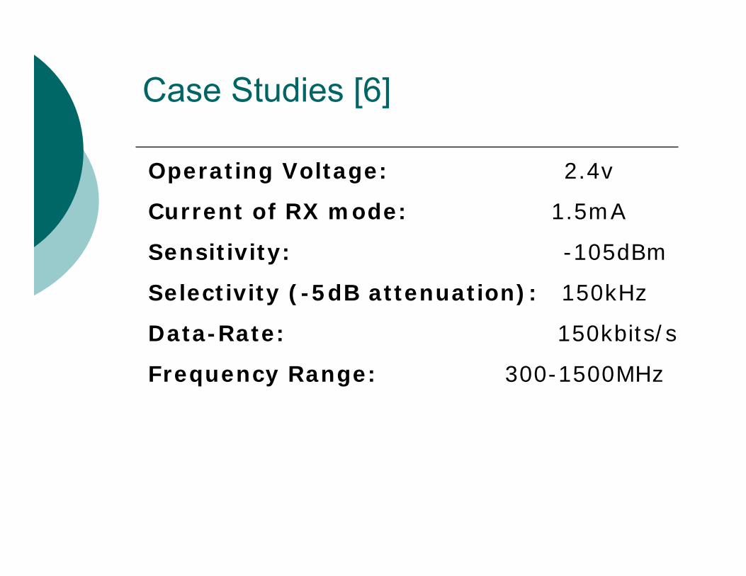
Case Studies [6]

Operating Voltage: 2.4v

Current of RX mode: 1.5mA

Sensitivity: -105dBm

Selectivity (-5dB attenuation): 150kHz

Data-Rate: 150kbits/s

Frequency Range: 300-1500MHz

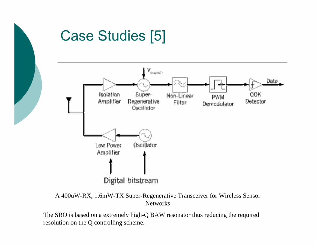
Case Studies [5]

A 400uW-RX, 1.6mW-TX Super-Regenerative Transceiver for Wireless Sensor Networks

The SRO is based on a extremely high-Q BAW resonator thus reducing the required resolution on the Q controlling scheme.

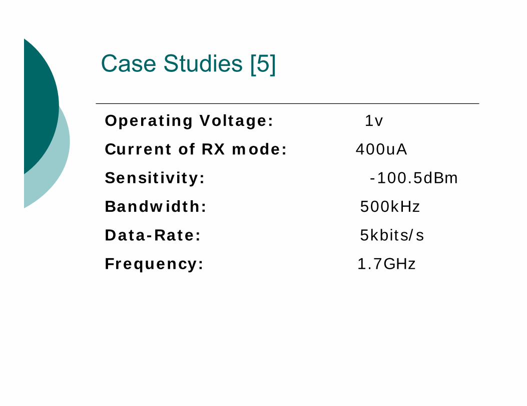
Case Studies [5]

Operating Voltage: 1v

Current of RX mode: 400uA

Sensitivity: -100.5dBm

Bandwidth: 500kHz

Data-Rate: 5kbits/s

Frequency: 1.7GHz

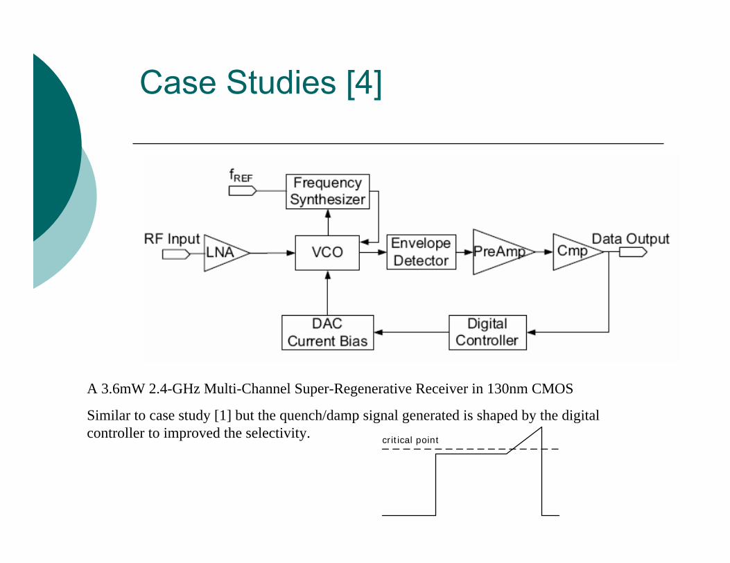
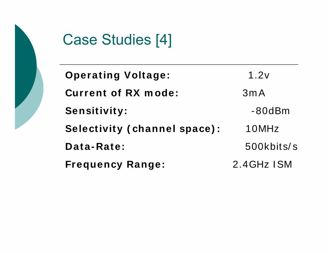
Case Studies [4]

A 3.6mW 2.4-GHz Multi-Channel Super-Regenerative Receiver in 130nm CMOS

Similar to case study [1] but the quench/damp signal generated is shaped by the digital controller to improved the selectivity. critical point

Case Studies [4]

Operating Voltage: 1.2v

Current of RX mode: 3mA

Sensitivity: -80dBm

Selectivity (channel space): 10MHz

Data-Rate: 500kbits/s

Frequency Range: 2.4GHz ISM

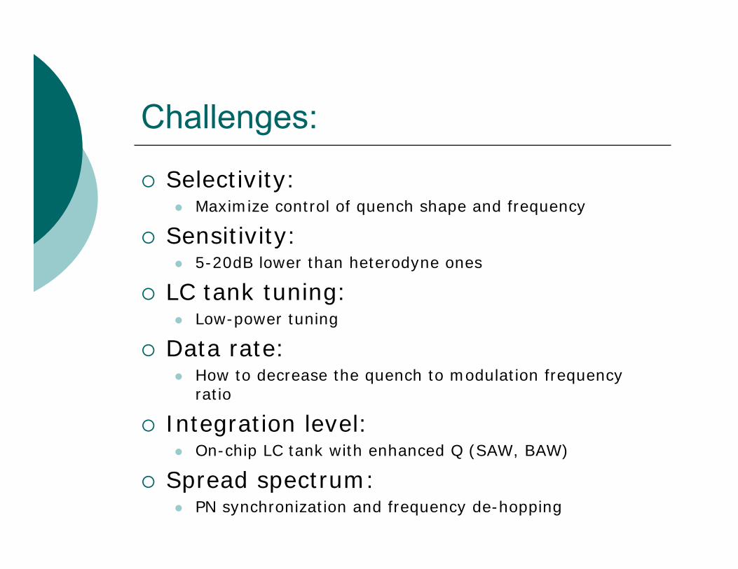
Challenges:

Selectivity: Maximize control of quench shape and frequency

Sensitivity: 5-20dB lower than heterodyne ones

LC tank tuning: Low-power tuning

Data rate: How to decrease the quench to modulation frequency ratio

Integration level: On-chip LC tank with enhanced Q (SAW, BAW)

Spread spectrum: PN synchronization and frequency de-hopping

References:

[1] E. H. Armstrong, “ Some recent developments of regenerative circuits,” Proc. IRE, vol. 10, pp. 244-260, Aug. 1922

[2] J. R. Whitehead, Super-Regenerative Receivers. Cambridge Univ. Press, 1950.[3] F.X. Moncunill-Geniz, P. Pala-Schonwalder, O. Mas-Casals, “A generic approach to the theory of

superregenerative reception,” IEEE Transactions on Circuits and Systems-I, vol. 52, No.1, pp:54 – 70, Jan. 2005.

[4] J.Y. Chen, M. P. Flynn, and J. P. Hayes, “A 3.6mW 2.4-GHz multi-channel super-regenerative receiver in 130nm CMOS,” In Proc. IEEE Custom Integrated Circ. Conference, pp. 361-364, Sep. 2005.

[5] B. Otis, Y. H. Chee, and Y. Rabaey, “A 400uW-RX, 1.6mW-TX super-regenerative transceiver for wireless sensor networks,” Digest of Technical Papers of the IEEE Int. Solid-State Circ. Conference, vol. 1, pp. 396-397 and p. 606, San Francisco, Feb. 2005.

[6] N. Joehl, C. Dehollain, P. Favre, P. Deval, M. Declerq, “A low-power 1-GHz super-regenerative transceiver with time-shared PLL control,” IEEE J. of Solid-State Circuits, vol. 36, pp:1025 – 1031, Jul. 2001.

[7] P. Favre, N. Joehl, A. Vouilloz, P. Deval, C. Dehollain, M.J. Declercq, “A 2-V 600-μA 1-GHz BiCMOS super-regenerative receiver for ISM applications,” IEEE J. of Solid-State Circuits, vol. 33, pp:2186 – 2196, Dec. 1998.

[8] F.X. Moncunill-Geniz, P. Pala-Schonwalder, C. Dehollain, N. Joehl, M. Declercq, “A 2.4-GHz DSSS superregenerative receiver with a simple delay-locked loop,” IEEE Microwave and Wireless Components Letters, vol 15, pp:499 – 501, Aug. 2005.

[9] A. Vouilloz, M. Declercq, C. Dehollain, “A low-power CMOS super-regenerative receiver at 1 GHz,” IEEE J.Solid-state circuits, vol. 36, pp:440 – 451, Mar. 2001.

[10] A. Vouilloz, M. Declercq, C. Dehollain, “Selectivity and sensitivity performances of superregenerativereceivers,” Proc. ISCAS’98, vol.4, pp:325-328, Jun. 1998.

[11] F.X. Moncunill-Geniz, C. Dehollain, N. Joehl, M. Declercq, P. Pala-Schonwalder, “A 2.4-GHz Low-Power Superregenerative RF Front-End for High Data Rate Applications,” Microwave Conference, 2006. 36th European, pp:1537 – 1540, Sept. 2006