6.1 Plate Theory - Auckland

Section 6.1

Solid Mechanics Part II Kelly 120

6.1 Plate Theory 6.1.1 Plates A plate is a flat structural element for which the thickness is small compared with the surface dimensions. The thickness is usually constant but may be variable and is measured normal to the middle surface of the plate, Fig. 6.1.1

Fig. 6.1.1: A plate 6.1.2 Plate Theory Plates subjected only to in-plane loading can be solved using two-dimensional plane stress theory1 (see Book I, §3.5). On the other hand, plate theory is concerned mainly with lateral loading. One of the differences between plane stress and plate theory is that in the plate theory the stress components are allowed to vary through the thickness of the plate, so that there can be bending moments, Fig. 6.1.2.

Fig. 6.1.2: Stress distribution through the thickness of a plate and resultant bending

moment Plate Theory and Beam Theory Plate theory is an approximate theory; assumptions are made and the general three dimensional equations of elasticity are reduced. It is very like the beam theory (see Book

1 although if the in-plane loads are compressive and sufficiently large, they can buckle (see §6.7)

middle surface of plate

lateral load

M

Section 6.1


I, §7.4) – only with an extra dimension. It turns out to be an accurate theory provided the plate is relatively thin (as in the beam theory) but also that the deflections are small relative to the thickness. This last point will be discussed further in §6.10. Things are more complicated for plates than for the beams. For one, the plate not only bends, but torsion may occur (it can twist), as shown in Fig. 6.1.3

Fig. 6.1.3: torsion of a plate

Assumptions of Plate Theory Let the plate mid-surface lie in the yx plane and the z – axis be along the thickness direction, forming a right handed set, Fig. 6.1.4.

Fig. 6.1.4: Cartesian axes The stress components acting on a typical element of the plate are shown in Fig. 6.1.5.

Fig. 6.1.5: stresses acting on a material element

y

x

xxyy

xy

zx yz

z

zz

x

y

z

Section 6.1


The following assumptions are made: (i) The mid-plane is a “neutral plane” The middle plane of the plate remains free of in-plane stress/strain. Bending of the plate will cause material above and below this mid-plane to deform in-plane. The mid-plane plays the same role in plate theory as the neutral axis does in the beam theory. (ii) Line elements remain normal to the mid-plane Line elements lying perpendicular to the middle surface of the plate remain perpendicular to the middle surface during deformation, Fig. 6.1.6; this is similar the “plane sections remain plane” assumption of the beam theory.

Fig. 6.1.6: deformed line elements remain perpendicular to the mid-plane (iii) Vertical strain is ignored Line elements lying perpendicular to the mid-surface do not change length during deformation, so that 0zz throughout the plate. Again, this is similar to an assumption of the beam theory. These three assumptions are the basis of the Classical Plate Theory or the Kirchhoff Plate Theory. The second assumption can be relaxed to develop a more exact theory (see §6.10). 6.1.3 Notation and Stress Resultants The stress resultants are obtained by integrating the stresses through the thickness of the plate. In general there will be moments M: 2 bending moments and 1 twisting moment out-of-plane forces V: 2 shearing forces in-plane forces N: 2 normal forces and 1 shear force

undeformed

line element remains perpendicular to mid-surface

Section 6.1


They are defined as follows: In-plane normal forces and bending moments, Fig. 6.1.7:

2/

2/

2/

2/

2/

2/

2/

2/

,

,

h

h

yyy

h

h

xxx

h

h

yyy

h

h

xxx

dzzMdzzM

dzNdzN

(6.1.1)

Fig. 6.1.7: in-plane normal forces and bending moments In-plane shear force and twisting moment, Fig. 6.1.8:

2/

2/

2/

2/

,h

h

xyxy

h

h

xyxy dzzMdzN (6.1.2)

Fig. 6.1.8: in-plane shear force and twisting moment Out-of-plane shearing forces, Fig. 6.1.9:

2/

2/

2/

2/

,h

h

yzy

h

h

zxx dzVdzV (6.1.3)

y

xxN

yN

xM

yMxx

yy

y

x

xyN

xyM

xyxy

xyN

xyM

Section 6.1


Fig. 6.1.9: out of plane shearing forces Note that the above “forces” and “moments” are actually forces and moments per unit length. This allows one to have moments varying across any section – unlike in the beam theory, where the moments are for the complete beam cross-section. If one considers an element with dimensions x and y , the actual moments acting on the element are

yMxMxMyM xyxyyx ,,, (6.1.4)

and the forces acting on the element are

yNxNxNyNxVyV xyxyyxyx ,,,,, (6.1.5)

The in-plane forces, which are analogous to the axial forces of the beam theory, do not play a role in most of what follows. They are useful in the analysis of buckling of plates and it is necessary to consider them in more exact theories of plate bending (see later).

y

x

yV

zx yz

yz

zx

xV

Section 6.2


6.2 The Moment-Curvature Equations 6.2.1 From Beam Theory to Plate Theory In the beam theory, based on the assumptions of plane sections remaining plane and that one can neglect the transverse strain, the strain varies linearly through the thickness. In the notation of the beam, with y positive up, Ryxx / , where R is the radius of

curvature, R positive when the beam bends “up” (see Book I, Eqn. 7.4.16). In terms of the curvature Rxv /1/ 22 , where v is the deflection (see Book I, Eqn. 7.4.36), one has

2

2

x

vyxx

(6.2.1)

The beam theory assumptions are essentially the same for the plate, leading to strains which are proportional to distance from the neutral (mid-plane) surface, z, and expressions similar to 6.2.1. This leads again to linearly varying stresses xx and yy ( zz is also

taken to be zero, as in the beam theory). 6.2.2 Curvature and Twist The plate is initially undeformed and flat with the mid-surface lying in the yx plane. When deformed, the mid-surface occupies the surface ),( yxww and w is the elevation above the yx plane, Fig. 6.2.1.

Fig. 6.2.1: Deformed Plate The slopes of the plate along the x and y directions are xw / and yw / .

x

y

initial position

w

Section 6.2


Curvature Recall from Book I, §7.4.11, that the curvature in the x direction, x , is the rate of change

of the slope angle with respect to arc length s, Fig. 6.2.2, dsdx / . One finds that

2 2

3/22

/

1 /x

w x

w x

(6.2.2)

Also, the radius of curvature xR , Fig. 6.2.2, is the reciprocal of the curvature, xxR /1 .

Fig. 6.2.2: Angle and arc-length used in the definition of curvature As with the beam, when the slope is small, one can take xw /tan and

xdsd // and Eqn. 6.2.2 reduces to (and similarly for the curvature in the y direction)

2

2

2

2 1,

1

y

w

Rx

w

R yy

xx

(6.2.3)

This important assumption of small slope, / , / 1w x w y , means that the theory to be developed will be valid when the deflections are small compared to the overall dimensions of the plate. The curvatures 6.2.3 can be interpreted as in Fig. 6.2.3, as the unit increase in slope along the x and y directions.

x

w s

xR

Section 6.2


Figure 6.2.3: Physical meaning of the curvatures Twist Not only does a plate curve up or down, it can also twist (see Fig. 6.1.3). For example, shown in Fig. 6.2.4 is a plate undergoing a pure twisting (constant applied twisting moments and no bending moments).

Figure 6.2.4: A twisting plate If one takes a row of line elements lying in the y direction, emanating from the x axis, the further one moves along the x axis, the more they twist, Fig. 6.2.4. Some of these line elements are shown in Fig. 6.2.5 (bottom right), as veiwed looking down the x axis towards the origin (elements along the y axis are shown bottom left). If a line element at position x has slope /w y , the slope at x x is / ( / ) /w y x w y x . This motivates the definition of the twist, defined analogously to the curvature, and denoted by

xyT/1 ; it is a measure of the “twistiness” of the plate:

yx

w

Txy

21

(6.2.4)

y

x

z

xyM

xyM

y

w

x

y

A B

C D

AB

w

y

2

2

w wy

y y

A

w

x

2

2

w wx

x x

x

C

w w

y

x

Section 6.2


Figure 6.2.5: Physical meaning of the twist The signs of the moments, radii of curvature and curvatures are illustrated in Fig. 6.2.6. Note that the deflection w may or may not be of the same sign as the curvature. Note also that when 0/,0 22 xM x , when 0/,0 22 yM y .

Figure 6.2.6: sign convention for curvatures and moments On the other hand, for the twist, with the sign convention being used, when

0/,0 2 yxM xy , as depicted in Fig. 6.2.4.

Principal Curvatures Consider the two Cartesian coordinate systems shown in Fig. 6.2.7, the second ( nt ) obtained from the first ( yx ) by a positive rotation . The partial derivatives arising in

0xR

0/ 22 x

0xR

0/ 22 x0xM

0xM

zx

zx

y

w

x

A B

C D

xyxy

2

yyxx

2

yA

BA

x

x

D

C

y

C B

D w w

Section 6.2


the curvature expressions can be expressed in terms of derivatives with respect to t and n as follows: with yxww , , an increment in w is

yy

wx

x

ww

(6.2.5)

Also, referring to Fig. 6.2.7, with 0n ,

sin,cos tytx (6.2.6) Thus

sincosy

w

x

w

t

w

(6.2.7)

Similarly, for an increment n , one finds that

cossiny

w

x

w

n

w

(6.2.8)

Equations 6.2.7-8 can be inverted to get the inverse relations

cossin

sincos

n

w

t

w

y

wn

w

t

w

x

w

(6.2.9)

Figure 6.2.7: Two different Cartesian coordinate systems The relationship between second derivatives can be found in the same way. For example,

nt

w

n

w

t

w

n

w

t

w

ntx

w

2

2

22

2

22

2

2

2sinsincos

sincossincos

(6.2.10)

x

n y

t

x

yt

o

Section 6.2


In summary, one has

nttnyx

w

ntnty

w

ntntx

w

2

2

2

2

22

2

2

22

2

22

2

2

2

2

22

2

22

2

2

2coscossin

2sincossin

2sinsincos

(6.2.11)

and the inverse relations

yxxynt

w

yxyxn

w

yxyxt

w

2

2

2

2

22

2

2

22

2

22

2

2

2

2

22

2

22

2

2

2coscossin

2sincossin

2sinsincos

(6.2.12)

or1

xyxytn

xyyxn

xyyxt

TRRT

TRRR

TRRR

12cos

11cossin

1

12sin

1cos

1sin

1

12sin

1sin

1cos

1

22

22

(6.2.13)

These equations which transform between curvatures in different coordinate systems have the same structure as the stress transformation equations (and the strain transformation equations), Book I, Eqns. 3.4.8. As with principal stresses/strains, there will be some angle for which the twist is zero; at this angle, one of the curvatures will be the minimum and one will be the maximum at that point in the plate. These are called the principal curvatures. Similarly, just as the sum of the normal stresses is an invariant (see Book I, Eqn. 3.5.1), the sum of the curvatures is an invariant2:

ntyx RRRR

1111 (6.2.14)

If the principal curvatures are equal, the curvatures are the same at all angles, the twist is always zero and so the plate deforms locally into the surface of a sphere.

1 these equations are valid for any continuous surface; Eqns. 6.2.12 are restricted to nearly-flat surfaces. 2 this is known as Euler’s theorem for curvatures

Section 6.2


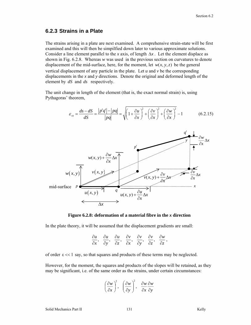
6.2.3 Strains in a Plate The strains arising in a plate are next examined. A comprehensive strain-state will be first examined and this will then be simpilfied down later to various approximate solutions. Consider a line element parallel to the x axis, of length x . Let the element displace as shown in Fig. 6.2.8. Whereas w was used in the previous section on curvatures to denote displacement of the mid-surface, here, for the moment, let ),,( zyxw be the general vertical displacement of any particle in the plate. Let u and v be the corresponding displacements in the x and y directions. Denote the original and deformed length of the element by dS and ds respectively. The unit change in length of the element (that is, the exact normal strain) is, using Pythagoras’ theorem,

2 2 2

1 1xx

p q pqds dS u v w

dS pq x x x

(6.2.15)

Figure 6.2.8: deformation of a material fibre in the x direction In the plate theory, it will be assumed that the displacement gradients are small:

, , , , , ,u u u v v v w

x y z x y z z

,

of order 1ε say, so that squares and products of these terms may be neglected. However, for the moment, the squares and products of the slopes will be retained, as they may be significant, i.e. of the same order as the strains, under certain circumstances:

y

w

x

w

y

w

x

w

,,22

p

( , )u

u x y xx

xx

w

x

pq ,u x y

q

,w x y

( , )w

w x y xx

mid-surface x

y

,v x y( , )

vv x y x

x

v

xx

Section 6.2


Eqn. 6.2.15 now reduces to

2

1 2 1xx

u w

x x

(6.2.16)

With 2/11 xx for 1x , one has (and similarly for the other normal strains)

z

w

y

w

y

v

x

w

x

u

zz

yy

xx

2

2

2

1

2

1

(6.2.17)

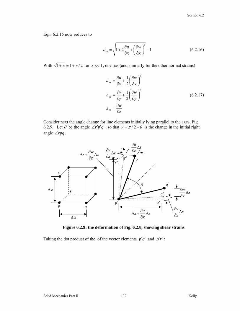
Consider next the angle change for line elements initially lying parallel to the axes, Fig. 6.2.9. Let be the angle qpr , so that 2/ is the change in the initial right angle rpq .

Figure 6.2.9: the deformation of Fig. 6.2.8, showing shear strains

Taking the dot product of the of the vector elements qp and rp :

p p q

q

r

s

x

xx

ux

xx

w

zz

v

r

z

zz

u

xx

v

r

q

q

r

zz

wz

Section 6.2


2 2 2 2 2

cos

1 1

p q r r q q r r q q p r

p q p r

u u v v w wx x z x z x z z

x z x z x z

u v w w ux z

x x x z z

2vz

(6.2.18)

Again, with the displacement gradients /u x , /v x , /u z , /v z , /w z of order

1ε (and the squares 2/w x at most of order 1ε ),

z

v

x

v

x

w

z

u

zx

zxx

wz

z

vx

x

vz

z

ux

cos (6.2.19)

For small , cossin , so (and similarly for the other shear strains)

y

w

z

v

x

w

z

u

y

w

x

w

x

v

y

u

yz

xz

xy

2

1

2

1

2

1

(6.2.20)

The normal strains 6.2.17 and the shear strains 6.2.20 are non-linear. They are the starting point for the various different plate theories. Von Kármán Strains Introduce now the assumptions of the classical plate theory. The assumption that line elements normal to the mid-plane remain inextensible implies that

0

z

wzz (6.2.21)

This implies that yxww , so that all particles at a given yx, through the thickness of the plate experinece the same vertical displacement. The assumption that line elements perpendicular to the mid-plane remain normal to the mid-plane after deformation then implies that 0 yzxz .

The strains now read

Section 6.2


0

0

2

1

0

2

1

2

1

2

2

yz

xz

xy

zz

yy

xx

y

w

x

w

x

v

y

u

y

w

y

v

x

w

x

u

(6.2.22)

These are known as the Von Kármán strains. Membrane Strains and Bending Strains Since 0xz and ),( yxww , one has from Eqn. 6.2.20b,

),(),,( 0 yxux

wzzyxu

x

w

z

u

(6.2.23)

It can be seen that the function ),(0 yxu is the displacement in the mid-plane. In terms of

the mid-surface displacements 000 ,, wvu , then,

00

00

0 ,, wwy

wzvv

x

wzuu

(6.2.24)

and the strains 6.2.22 may be expressed as

yx

wz

y

w

x

w

x

v

y

u

y

wz

y

w

y

v

x

wz

x

w

x

u

xy

yy

xx

02

0000

20

22

00

20

22

00

2

1

2

1

2

1

2

1

(6.2.25)

The first terms are the usual small-strains, for the mid-surface. The second terms, involving squares of displacement gradients, are non-linear, and need to be considered when the plate bending is fairly large (when the rotations are about 10 – 15 degrees). These first two terms together are called the membrane strains. The last terms, involving second derivatives, are the flexural (bending) strains. They involve the curvatures. When the bending is not too large (when the rotations are below about 10 degrees), one has (dropping the subscript “0” from w)

Section 6.2


yx

wz

x

v

y

u

y

wz

y

vx

wz

x

u

xy

yy

xx

200

2

20

2

20

2

1

(6.2.26)

Some of these strains are illustrated in Figs. 6.2.10 and 6.2.11; the physical meaning of

xx is shown in Fig. 6.2.10 and some terms from xy are shown in Fig. 6.2.11.

Figure 6.2.10: deformation of material fibres in the x direction

Figure 6.2.11: the deformation of 6.2.10 viewed “from above”; a , b are the deformed positions of the mid-surface points a, b

p

pa, qb,

q

b

ax

yx

wz

y

wz

2

x

x

vv

00

y

wzv

0

c0v

p

a

x

w

w

xx

ww

xx

w

x

w

2

2

x

a

p

b

q

x

wzu

0

0u

xx

uu

00

xx

wz

x

u

x

wzu

2

20

0

q

bq

mid-surface

z

xx

Section 6.2


Finally, when the mid-surface strains are neglected, according to the final assumption of the classical plate theory, one has

yx

wz

y

wz

x

wz xyyyxx

2

2

2

2

2

,, (6.2.27)

In summary, when the plate bends “up”, the curvature is positive, and points “above” the mid-surface experience negative normal strains and points “below” experience positive normal strains; there is zero shear strain. On the other hand, when the plate undergoes a positive pure twist, so the twisting moment is negative, points “above” the mid-surface experience negative shear strain and points “below” experience positive shear strain; there is zero normal strain. A pure shearing of the plate in the x y plane is illustrated in Fig. 6.2.12.

Figure 6.2.12: Shearing of the plate due to a positive twist (neative twisting moment) Compatibility Note that the strain fields arising in the plate satisfy the 2D compatibility relation Eqn. 1.3.1:

yxxyxyyyxx

2

2

2

2

2

2 (6.2.28)

This can be seen by substituting Eqn. 6.25 (or Eqns 6.26-27) into Eqn. 6.2.28. 6.2.4 The Moment-Curvature equations Now that the strains have been related to the curvatures, the moment-curvature relations, which play a central role in plate theory, can be derived.

x

y

mid-surface

bottom

top

Section 6.2


Stresses and the Curvatures/Twist in a Linear Elastic Plate From Hooke’s law, taking 0zz ,

xyxyxxyyyyyyxxxx EEEEE

1

,1

,1

(6.2.29)

so, from 6.2.27, and solving 6.2.29a-b for the normal stresses,

yx

wz

E

x

w

y

wz

E

y

w

x

wz

E

xy

yy

xx

2

2

2

2

2

2

2

2

2

2

2

1

1

1

(6.2.30)

The Moment-Curvature Equations Substituting Eqns. 6.2.30 into the definitions of the moments, Eqns. 6.1.1, 6.1.2, and integrating, one has

yx

wDM

x

w

y

wDM

y

w

x

wDM

xy

y

x

2

2

2

2

2

2

2

2

2

1

(6.2.31)

where

2

3

112

EhD (6.2.32)

Equations 6.2.31 are the moment-curvature equations for a plate. The moment-curvature equations are analogous to the beam moment-deflection equation

EIMxv // 22 . The factor D is called the plate stiffness or flexural rigidity and plays the same role in the plate theory as does the flexural rigidity term EI in the beam theory. Stresses and Moments From 6.30-6.31, the stresses and moments are related through

12/,

12/,

12/ 333 h

zM

h

zM

h

zM xyxy

yyy

xxx (6.2.33)

Section 6.2


Note the similarity of these relations to the beam formula IMy / with 12/3hI times the width of the beam. 6.2.5 Principal Moments It was seen how the curvatures in different directions are related, through Eqns. 6.2.11-12. It comes as no surprise, examining 6.2.31, that the moments are related in the same way. Consider a small differential element of a plate, Fig. 6.2.13a, subjected to stresses xx ,

yy , xy , and corresponding moments xyyx MMM ,, given by 6.1.1-2. On any

perpendicular planes rotated from the orginal yx axes by an angle , one can find the

new stresses tt , nn , tn , Fig. 6.2.13b (see Fig. 6.2.5), through the stress

transformatrion equations (Book I, Eqns. 3.4.8). Then

xyyx

xyyyxxttt

MMM

dzzdzzdzzdzzM

2sinsincos

2sinsincos

22

22

(6.2.34)

and similarly for the other moments, leading to

xyxytn

xyyxn

xyyxt

MMMM

MMMM

MMMM

2cossincos

2sincossin

2sinsincos22

22

(6.2.35)

Also, there exist principal planes, upon which the shear stress is zero (right through the thickness). The moments acting on these planes, 1M and 2M , are called the principal moments, and are the greatest and least bending moments which occur at the element. On these planes, the twisting moment is zero.

Figure 6.2.13: Plate Element; (a) stresses acting on element, (b) rotated element

xx

xy

xy

nntt

tn

Section 6.2


Moments in Different Coordinate Systems From the moment-curvature equations 6.2.31, {▲Problem 1}

2 2

2 2

2 2

2 2

2

1

t

n

tn

M Dt n

M Dn t

M Dt n

(6.2.36)

showing that the moment-curvature relations 6.2.31 hold in all Cartesian coordinate systems. 6.2.6 Problems 1. Use the curvature transformation relations 6.2.11 and the moment transformation

relations 6.2.35 to derive the moment-curvature relations 6.2.36.

Section 6.3


6.3 Plates subjected to Pure Bending and Twisting 6.3.1 Pure Bending of an Elastic Plate Consider a plate subjected to bending moments 1 0xM M= > and 2 0yM M= > , with no other loading, as shown in Fig. 6.3.1.

Figure 6.3.1: A plate under Pure Bending From equilibrium considerations, these moments act at all points within the plate – they are constant throughout the plate. Thus, from the moment-curvature equations 6.2.31, one has the set of coupled partial differential equations

yxw

xw

yw

DM

yw

xw

DM

∂∂∂

=∂∂

+∂∂

=∂∂

+∂∂

=2

2

2

2

22

2

2

2

21 0,, νν (6.3.1)

Solving for the derivatives,

0,)1(

,)1(

2

212

2

2

221

2

2

=∂∂

∂−−

=∂∂

−−

=∂∂

yxw

DMM

yw

DMM

xw

νν

νν (6.3.2)

Integrating the first two equations twice gives1

)()()1(2

1),()()1(2

121

22

1221

22

21 xgyxgyD

MMwyfxyfxD

MMw ++−−

=++−−

=νν

νν (6.3.3)

and integrating the third shows that two of these four unknown functions are constants:

BxgAyfyFywxG

xw

==→=∂∂

=∂∂ )(,)()(),( 11 (6.3.4)

1 this analysis is similar to that used to evaluate displacements in plane elastostatic problems, §1.2.4

y

x1M

1M

2M2M

Section 6.3


Equating both expressions for w in 6.3.3 gives

)()1(2

1)()1(2

12

22

122

22

21 yfByyD

MMxgAxxD

MM−+

−−

=−+−−

νν

νν (6.3.5)

For this to hold, both sides here must be a constant, C− say. It follows that

CByAxyD

MMxD

MMw +++−−

+−−

= 22

1222

21

)1(21

)1(21

νν

νν (6.3.6)

The three unknown constants represent an arbitrary rigid body motion. To obtain values for these, one must fix three degrees of freedom in the plate. If one supposes that the deflection w and slopes ywxw ∂∂∂∂ /,/ are zero at the origin 0== yx (so the origin of the axes are at the plate-centre), then 0=== CBA ; all deformation will be measured relative to this reference. It follows that

( )[ ] ( )[ ][ ]221

2212

2 /1/)1(2

yMMxMMD

Mw ννν

−+−−

= (6.3.7)

Once the deflection w is known, all other quantities in the plate can be evaluated – the strain from 6.2.27, the stress from Hooke’s law or directly from 6.2.30, and moments and forces from 6.1.1-3. In the special case of equal bending moments, with oMMM == 21 say, one has

( )22

)1(2yx

DM

w o ++

=ν

(6.3.8)

This is the equation of a sphere. In fact, from the relationship between the curvatures and the radius of curvature R,

constant)1()1(2

2

2

2

=+

=→+

=∂∂

=∂∂

o

o

MDR

DM

yw

xw ν

ν (6.3.9)

and so the mid-surface of the plate in this case deforms into the surface of a sphere with radius given by 6.3.9, as illustrated in Fig. 6.3.2.

Figure 6.3.2: Deformed plate under Pure Bending with equal moments

Section 6.3


The character of the deformed plate is plotted in Fig. 6.3.3 for various ratios 12 / MM (for 3.0=ν ).

Figure 6.3.3: Bending of a Plate When the curvatures 22 / xw ∂∂ and 22 / yw ∂∂ are of the same sign2, the deformation is called synclastic. When the curvatures are of opposite sign, as in the lower plots of Fig. 6.3.3, the deformation is said to be anticlastic. Note that when there is only one moment, 0=yM say, there is still curvature in both directions. In this case, one can solve the moment-curvature equations to get

( ) ( ) ( )2 2 2

2 22 2 22 2

, ,1 2 1

x xM Mw w w w x yx y xD D

ν νν ν

∂ ∂ ∂= = − = −

∂ ∂ ∂− − (6.3.10)

which is an anticlastic deformation. In order to get a pure cylindrical deformation, )(xfw = say, one needs to apply moments

xM and xy MM ν= , in which case, from 6.3.6,

2 or principal curvatures in the case of a more complex general loading

5.1/ 12 =MM 3/ 12 =MM

5.1/ 12 −=MM 3/ 12 −=MM

Section 6.3


2

2x

DM

w x= (6.3.11)

The deformation for 3/ 12 =MM in Fig. 6.3.3 is very close to cylindrical, since there

yx MM ν≈ for typical values of ν . 6.3.2 Pure Torsion of an Elastic Plate In pure torsion, one has the twisting moment 0xyM M= > with no other loading, Fig. 6.3.4. From the moment-curvature equations,

yxw

DM

xw

yw

yw

xw

∂∂∂

=−

−∂∂

+∂∂

=∂∂

+∂∂

=2

2

2

2

2

2

2

2

2

)1(,0,0

ννν (6.3.12)

so that

)1(,0,0

2

2

2

2

2

ν−−=

∂∂∂

=∂∂

=∂∂

DM

yxw

yw

xw (6.3.13)

Figure 6.3.4: Twisting of a Plate Using the same arguments as before, integrating these equations leads to

xyD

Mw)1( ν−

−= (6.3.14)

The middle surface is deformed as shown in Fig. 6.3.5, for a negative xyM . Note that there is no deflection along the lines 0=x or 0=y . The principal curvatures will occur at 45o to the axes (see Eqns. 6.2.13):

y

x

M

M

Section 6.3


)1(1,

)1(1

21 νν −−=

−+=

DM

RDM

R (6.3.15)

Figure 6.3.5: Deformation for a (negative) twisting moment

y

x

2R

Section 6.4


6.4 Equilibrium and Lateral Loading In this section, lateral loads are considered and these lead to shearing forces yx VV , , in the

plate. 6.4.1 The Governing Differential Equation for Lateral Loads In general, a plate will at any location be subjected to a lateral pressure q , bending

moments xyyx MMM ,, and out-of-plane shear forces xV and yV ; q is the normal pressure

on the upper surface of the plate:

2/),,(

2/,0),(

hzyxq

hzyxzz (6.4.1)

These quantities are related to each other through force equilibrium. Force Equilibrium Consider a differential plate element with one corner at )0,0(),( yx , Fig. 6.4.1, subjected to moments, pressure and shear force. Taking force equilibrium in the vertical direction (neglecting a possible small variation in q, since this will only introduce higher order terms):

0

yxqyx

x

VVyVxy

y

VVxVF x

xxy

yyz (6.4.2)

Fig. 6.4.1: a plate element subjected to moments, pressure and shear forces Eqn. 6.4.2 gives the vertical equilibrium equation

qy

V

x

V yx

(6.4.3)

y

x

yyM y

q

yyVy

yyM xy

xxM x

xxVx xxM xy

Section 6.4


This is analogous to the beam theory equation /p dV dx (see Book I, §7.4.3). Next, taking moments about the x axis:

02/2/

2/

yxqyyyxx

VVyy

yVyyxyy

VVyyxyV

xyy

MMxMyx

x

MMyMM

xx

xy

yy

yyy

xyxyxyx

(6.4.4)

Using 6.4.3, this reduces to (and similarly for moments about the x-axis),

y

M

x

MV

y

M

x

MV

yxyy

xyxx

(6.4.5)

These are analogous to the beam theory equation dxdMV / (see Book I, §7.4.3). Relations directly from the Equations of Equilibrium The equilibrium relations 6.4.3, 6.4.5 can also be derived directly from the equations of equilibrium, Eqns. 1.1.9, which encompass the force balances:

0

0

0

zyx

zyx

zyx

zzyzxz

zyyyxy

zxyxxx

(6.4.6)

Taking the first of these (which ensures equilibrium of forces in the x direction), multiplying by z and integrating over the plate thickness, gives

0

0

2/

2/

2/

2/

2/

2/

2/

2/

2/

2/

2/

2/

2/

2/

dzzdzzy

dzzx

dzz

zdzy

zdzx

z

h

h

zxh

hzx

h

h

yx

h

h

xx

h

h

zxh

h

yxh

h

xx

(6.4.7)

and, since the shear stress zx must be zero over the top and bottom surfaces, one has

Eqn. 6.4.5a. Applying a similar procedure to the second equilibrium equation gives Eqn.

Section 6.4


6.4.5b. Finally, integrating directly the third equilibrium equation without multiplying across by z, one arrives at Eqn. 6.4.3. Now, eliminating the shear forces from 6.4.3, 6.4.5 leads to the differential equation

qy

M

yx

M

x

M yxyx

2

22

2

2

2 (6.4.8)

This equation is analogous to the equation pxM 22 / in the beam theory. Finally, substituting in the moment-curvature equations 6.2.31 leads to1

D

q

y

w

yx

w

x

w

4

4

22

4

4

4

2 (6.4.9)

This is sometimes called the equation of Sophie Germain after the French investigator who first obtained it in 18152. This partial differential equation is solved subject to the boundary conditions of the problem, i.e. the fixing conditions of the plate (see below). Again, when once an expression for ),( yx is obtained, the strains, stresses, forces and moments follow. Note that the differential equation 6.4.8 with 0q is trivially satisfied in the simple pure bending and torsion problems considered earlier. Eqn. 6.4.9 can be succinctly expressed as

D

qw 4 (6.4.10)

where 2 is the Laplacian, or “del” operator:

2

2

2

22

yx

(6.4.11)

Note that the Laplacian operator (on w) gives the sum of the curvatures in two perpendicular directions and so it is independent of the directions chosen (see Eqn. 6.2.14). Shear Forces in terms of Deflection From 6.4.5 and the moment-curvature equations, one has the useful relations

1 note that the moment curvature relations were derived for the case of pure bending; here, as in the beam theory, the possible effect of the shearing forces on the curvature is neglected. This is a valid assumption provided the thickness of the plate is small in comparison with its other dimensions. A more exact theory taking into account the effect of the shear forces on deflection can be developed 2 Germain submitted her work to the French Academy, which was awarding a prize for anyone who could solve the problem of the vibration of plates; Lagrange was on the Academy awarding committee and corrected some of her work, deriving Eqn. 6.4.9 in its final form

Section 6.4


2

2

2

2

2

2

2

2

,y

w

x

w

yDV

y

w

x

w

xDV yx (6.4.12)

6.4.2 Stresses in the Plate The normal and in-plane shear stresses have been expressed in terms of the moments, Eqns. 6.2.33. Note that these stresses are zero over the mid-surface and attain a maximum at the outer surfaces. Expressions for the remaining stress components can be obtained from the equations of equilibrium as follows: the first of Eqns. 6.4.6 leads, with 6.4.5a, to

zV

h

z

zy

M

x

M

h

z

zM

h

z

yM

h

z

x

zyx

zxx

zxxyx

zxxyx

zxxyxx

3

3

33

12

12

1212

0

(6.4.13)

Integrating now gives (note that xV is independent of z)

CzVh xzx 2

3

6 (6.4.14)

This shear stress must be zero at the upper and lower (free –) surfaces, at 2/hz . This condition can be used to determine the arbitrary constant C and one finds that (see Fig. 6.1.9)

2

2/1

2

3

h

z

h

Vxzx (6.4.15)

The other shear stress, zy , can be evaluated in a similar manner: {▲Problem 1}

2

2/1

2

3

h

z

h

Vyzy (6.4.16)

In some analyses, these shear stresses are taken to be zero, although they can be quite significant.

Section 6.4


The only remaining stress component is zz . This will never exceed the intensity of the external load on the plate; the lateral load itself, however, is negligibly small in comparison with the in-plane stresses set up by the bending of the plate, and for this reason it is acceptable to disregard zz , as has been done, in the plate theory. 6.4.3 Problems 1. Derive the expression for shear stress 6.4.16.

Section 6.5


6.5 Plate Problems in Rectangular Coordinates In this section, a number of important plate problems will be examined using Cartesian coordinates. 6.5.1 Uniform Pressure producing Bending in One Direction Consider first the case of a plate which bends in one direction only. From 6.3.11 the deflection and moments are

2

2

2

2

)(,)(),(dx

wdDxM

dx

wdDxMxfw yx (6.5.1)

The differential equation 6.4.9 reads

D

xq

dx

wd )(4

4

(6.5.2)

The corresponding equation for a beam is EIxpdxwd /)(/ 44 . If )(/)( xqbxp ,

with b the depth of the beam, with 12/3bhI , the plate will respond more stiffly than the beam by a factor of )1/(1 2 , a factor of about 10% for 3.0 , since

b

EIEhD

22

3

1

1

112

(6.5.3)

The extra stiffness is due to the constraining effect of yM , which is not present in the

beam. 6.5.2 Deflection of a Circular Plate by a Uniform Lateral Load A solution for a circular plate problem is presented next. This problem will be examined again in the section which follows using the more natural polar coordinates. Consider a circular plate with boundary

222 ayx , (6.5.4) clamped at its edges and subjected to a uniform lateral load q, Fig. 6.5.1.

Section 6.5


Figure 6.5.1: a clamped circular plate subjected to a uniform lateral load The differential equation for the problem is given by 6.4.9. The boundary conditions are that the slope and deflection are zero at the boundary:

222along0,0,0 ayxy

w

x

ww

(6.5.5)

It will be shown that the deflection

2222 )( ayxcw (6.5.6) is a solution to the problem. First, this function certainly satisfies 6.5.5. Further, letting

222),( ayxyxf , (6.5.7) the relevant partial derivatives are

cy

wc

yx

wc

x

w

cyy

wcx

yx

wcy

yx

wcx

x

w

fycy

wcxy

yx

wfxc

x

w

cyfy

wcxf

x

w

24,8,24

24,8,8,24

24,8,24

4,4

4

4

22

4

4

4

3

3

2

3

2

3

3

3

22

222

2

2

(6.5.8)

Substituting these into the differential equation now yields

D

qc

64 (6.5.9)

so the deflection is

2222 )(64

ayxD

qw (6.5.10)

x

ya

q

Section 6.5


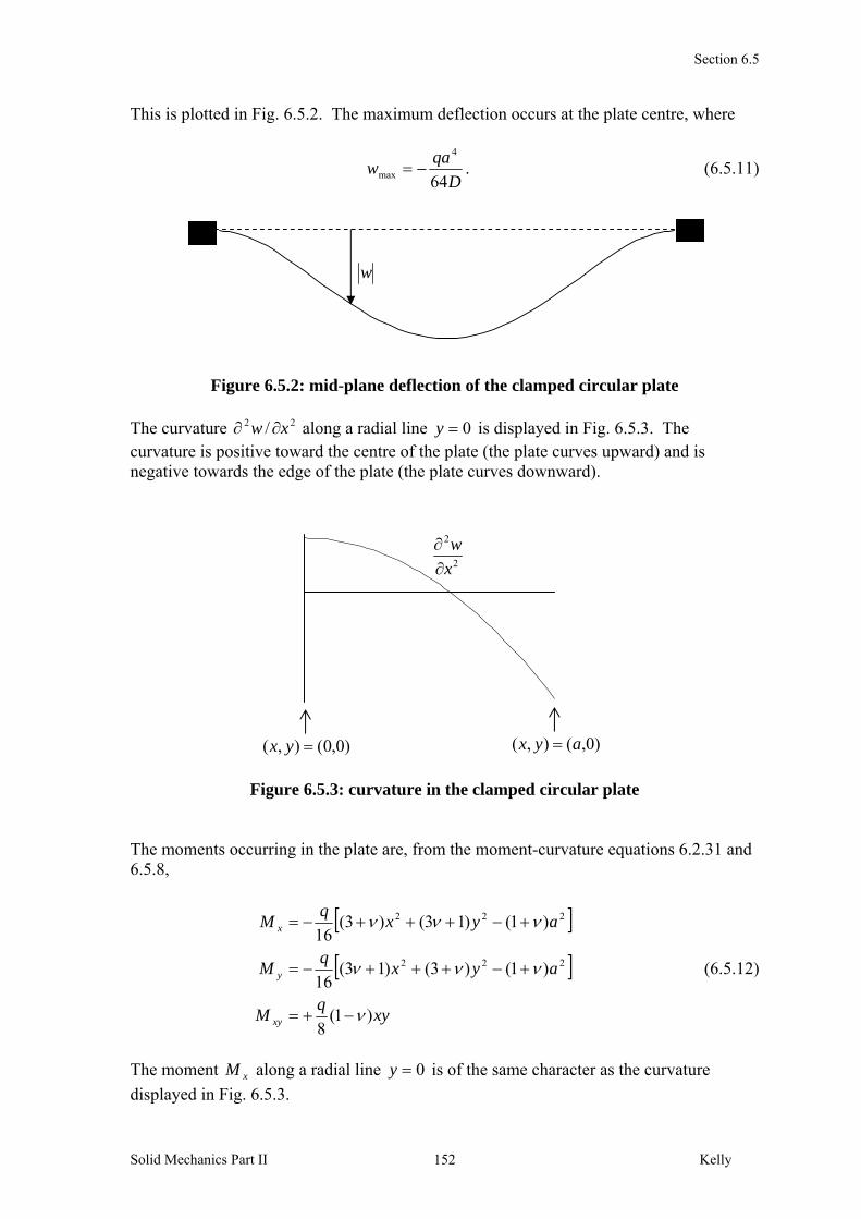
This is plotted in Fig. 6.5.2. The maximum deflection occurs at the plate centre, where

D

qaw

64

4

max . (6.5.11)

Figure 6.5.2: mid-plane deflection of the clamped circular plate The curvature 22 / xw along a radial line 0y is displayed in Fig. 6.5.3. The curvature is positive toward the centre of the plate (the plate curves upward) and is negative towards the edge of the plate (the plate curves downward).

Figure 6.5.3: curvature in the clamped circular plate The moments occurring in the plate are, from the moment-curvature equations 6.2.31 and 6.5.8,

xyq

M

ayxq

M

ayxq

M

xy

y

x

)1(8

)1()3()13(16

)1()13()3(16

222

222

(6.5.12)

The moment xM along a radial line 0y is of the same character as the curvature

displayed in Fig. 6.5.3.

2

2

x

w

)0,0(),( yx )0,(),( ayx

w

Section 6.5


The out-of-plane shear forces are, from 6.4.5,

2,

2

qyV

qxV yx (6.5.13)

At the plate centre, the expressions become

0,)1(16

2 yxxyyx VVMaq

MM (6.5.14)

Stresses in the Plate From 6.5.12-13 and 6.2.33, 6.4.15-16, the stresses in the plate are

2

2

3

2223

2223

2/1

4

3

2/1

4

3

)1(2

3

)1()3()13(4

3

)1()13()3(4

3

h

z

h

qy

h

z

h

qx

xyh

qz

ayxh

qz

ayxh

qz

zy

zx

xy

yy

xx

(6.5.15)

Converting to polar coordinates ),( r through

sin,cos ryrx (6.5.16) and using a stress transformation,

xyxxyyr

xyyyxx

xyyyxxrr

2cossincos

2sinsincos

2sinsincos22

22

(6.5.17)

leads to the axisymmetric stress field {▲Problem 1}

0

)1()13(4

3

)1()3(4

3

223

223

r

rr

arh

qz

arh

qz

(6.5.18)

Section 6.5


At the plate centre,

14

33

2

h

qzarr (6.5.19)

At the plate edge ar ,

3

2

3

2

2

3,

2

3

h

qza

h

qzarr (6.5.20)

For the shear stress, the traction acting on a surface parallel to the yx plane can be expressed as (see Fig. 6.5.4)

eeee

ee

eet

cossinsincos

rzyrzx

yzyxzx

zrzr

(6.5.21)

where ie is a unit vector in the direction i. Thus

0cossin

2/1

4

3sincos

2

zyzxz

zyzxzr h

z

h

qr

(6.5.22)

Figure 6.5.4: stress components acting on a surface Note that the maximum stress in the plate is

2

max 4

32/,

h

aqharr (6.5.23)

The maximum shear stress, on the other hand, is haqazr /4/3)0,( . Thus the shear stress is of an order ah / smaller than the normal stress.

zyy ,e

z,e

zrr ,ezxx ,e

Section 6.5


6.5.3 An Infinite Plate with Sinusoidal Deflection Consider next the classic plate problem addressed by Navier in 1820. It consists of an infinite plate with an undulating “up/down” sinusoidal deflection, Fig. 6.5.5,

b

y

a

xwyxw

sinsin),( 0 (6.5.24)

Figure 6.5.5: A plate with sinusoidal deflection Differentiation of the deflection leads to the curvatures

b

y

a

x

abw

xy

w

b

y

a

x

bw

y

w

b

y

a

x

aw

x

w

coscos

sinsin

sinsin

2

0

2

2

2

02

2

2

2

02

2

(6.5.25)

and hence the pressure

D

yxqyxw

bay

w

xy

w

x

w ),(),(

112

2

224

2

22

4

4

(6.5.26)

The pressure thus varies like the deflection. There is no need for supports for the plate since the “up” loads balance the “down” loads. From the moment-curvature relations,

x

y

a

b

Section 6.5


b

y

a

x

abDwM

b

y

a

x

baDwM

b

y

a

x

baDwM

xy

y

x

coscos1

sinsin1

sinsin1

2

0

222

0

222

0

(6.5.27)

and, from 6.4.12, the shear forces are

b

y

a

x

babDwV

b

y

a

x

baaDwV

y

x

cossin111

sincos111

223

0

223

0

(6.5.28)

Note that both wq / and yx MM / are constant throughout the plate.

6.5.4 A Simply Supported Plate with Sinusoidal Deflection Following on from the previous example, consider now a finite plate of dimensions a and b with the same sinusoidal deflection 6.5.24, simply supported along the edges 0x ,

ax , 0y , by . In what follows, take 0w in 6.5.24 to be negative, so that the plate

is pushed down towards the centre. According to 6.5.24 and 6.5.27, the deflection and slope is zero along the supported edges, as required. The vertical reactions at the supports are given by 6.5.28. However, according to Eqn. 6.5.27c, there are varying non-zero twisting moments over the ends of the plate. Thus the solution given by 6.5.24-28 is not quite the solution to the simply supported finite-plate problem, unless one can somehow apply the exact required twisting moments over the edges of the plate. It turns out, however, that the solution 6.5.24-28 is a correct solution, except in a region close to the edges of the plate. This is explained in what follows. Twisting Moments over “Free” Surfaces Consider an element of material of width dy , Fig. 6.5.6. The element is subjected to a

twisting moment dyM xy , Fig. 6.5.6a. This twisting moment is due to shear stresses

acting parallel to the plate surface (see Fig. 6.1.8). This system of horizontal forces can be replaced by the statically equivalent system of vertical forces shown in Fig. 6.5.6b – two forces of magnitude xyM separate by a distance dy . Recalling Saint-Venant’s

principle, the difference between the statically equivalent systems of forces of Fig. 6.5.6a and 6.5.6b will lead to differences in the stress field within the plate only in a small region very close to the plate-edges.

Section 6.5


Figure 6.5.6: Equivalent systems of forces leading to the same twisting moment; (a)

horizontal forces, (b) vertical forces Consider next a distribution of twisting moment along the plate edge, Fig. 6.5.7. As can be seen, this distribution is equivalent to a distribution of shearing forces (per unit length) of magnitude

y

MyV xy

x

)( (6.5.29)

Figure 6.5.7: A distribution of twisting moments along a plate edge The total vertical reaction along the edges can now be taken to be

y

MV xy

x

(6.5.30)

(and xMV xyy / along the other edges) and this gives a correct solution to the

problem. From 6.5.27-28, these reactions are

dyM xy

dy

xyM

y

MM xy

xy

dyy

MM xy

xy

dyM xy

dy

xyMxyM

(a) (b)

Section 6.5


a

x

ababDw

x

MVF

a

x

ababDw

x

MVF

b

y

bbaaDw

y

MVF

b

y

bbaaDw

y

MVF

bx

xyyyb

x

xyyy

ya

xyxxa

y

xyxx

sin1111

sin1111

sin1111

sin1111

2223

0

),(

2223

0

)0,(

0

2223

0

),(

2223

0

),0(

0

(6.5.31)

Corner Forces Integrating 6.5.31 over the four edges, the resultant upward forces on the four edges (with

00 w , they are all four upward) are

2222

00

2222

0x0

1112

1112

abab

aDwFF

bbaa

bDwFF

yby

xa

(6.5.32)

and the resultant of these may be expressed as

22

2

222

0up

12114

babaabDwF

(6.5.33)

The resultant downward force is, using 6.5.26,

2

222

0

0 0

2

224

0

0 0

down

114

sinsin11

),(

baabDw

dydxb

y

a

x

baDwdydxyxqF

b ab a

(6.5.34)

The difference between upF and downF is due to the re-distributed twisting moment, and is

explained a follows: consider again Fig. 6.5.7, where the edge twisting moments have been replaced with a statically equivalent distribution of shear forces. It can be seen that there results shear forces at the ends of the plate-edge (the “corners”), where the shear forces xyM have no neighbouring shear force of opposite sign with which to “cancel out”.

There are concentrated forces (per unit length) at the plate-corners of magnitude xyM .

Examining Fig. 6.5.7, which shows the edge ax , the force )0,(aM xy is positive up

whereas the force ),( baM xy is positive down. There are also contributions to the corner

Section 6.5


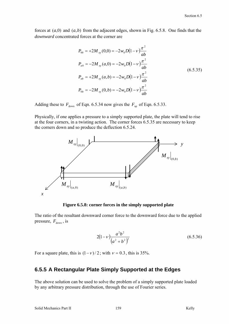
forces at )0,(a and ),( ba from the adjacent edges, shown in Fig. 6.5.8. One finds that the downward concentrated forces at the corner are

ab

DwbMP

abDwbaMP

abDwaMP

abDwMP

xyb

xyab

xya

xy

2

00

2

0

2

00

2

000

12),0(2

12),(2

12)0,(2

12)0,0(2

(6.5.35)

Adding these to downF of Eqn. 6.5.34 now gives the upF of Eqn. 6.5.33.

Physically, if one applies a pressure to a simply supported plate, the plate will tend to rise at the four corners, in a twisting action. The corner forces 6.5.35 are necessary to keep the corners down and so produce the deflection 6.5.24.

Figure 6.5.8: corner forces in the simply supported plate The ratio of the resultant downward corner force to the downward force due to the applied pressure, downF , is

222

22

12ba

ba

(6.5.36)

For a square plate, this is 2/)1( ; with 3.0 , this is 35%.

6.5.5 A Rectangular Plate Simply Supported at the Edges The above solution can be used to solve the problem of a simply supported plate loaded by any arbitrary pressure distribution, through the use of Fourier series.

y

x)0,(axyM

),( baxyM

),0( bxyM

)0,0(xyM

Section 6.5


Consider again this plate, whose displacement boundary conditions are

0,0

0,0,,,0

,2

2

0,2

2

,2

2

,02

2

bxxyayy

w

y

w

x

w

x

w

bxwxwyawyw

(6.5.37)

Assume the deflection to be of the form

1 1

sinsin),(m n

mn b

yn

a

xmAyxw

(6.5.38)

with mnA coefficients to be determined. It can be seen that this function satisfies the

boundary conditions. Taking the derivatives of this function,

1 12

22

2

2

sinsinm n

mn b

yn

a

xmA

a

m

x

w (6.5.39)

etc., and substituting into the differential equation 6.4.9, gives

1 1

2

2

2

2

24 ),(sinsin

m nmn yxq

b

yn

a

xm

b

n

a

mAD

(6.5.40)

This can be written compactly in the form

1 1

),(sinsinm n

mn yxqb

yn

a

xmC

(6.5.41)

where

2

2

2

2

24

b

n

a

mDAC mnmn (6.5.42)

It remains to choose the coefficients of the series so as to satisfy the equation identically over the whole area of the plate. One can evaluate the coefficients as one does for ordinary Fourier series, although here one has a double series and so one proceeds as follows: first, multiply both sides of (6.5.40) by byk /sin where k is an integer, and integrate over y between the limits

],0[ b , so that

1 1 00

sin),(sinsinsinm n

bb

mn dyb

ykyxqdy

b

yk

b

yn

a

xmC

(6.5.43)

Using the orthogonality condition

Section 6.5


knb

kndy

b

yk

b

ynb

,2/

,0sinsin

0

, (6.5.44)

leads to

1 0

sin),(sin2 m

b

mk dyb

ykyxq

a

xmC

b (6.5.45)

Now there are functions of x only so, multiplying both sides by )/sin( axj and following the same procedure, one has

a b

jk dxa

xjdy

b

ykyxqC

ba

0 0

sinsin),(22

(6.5.46)

and hence the coefficients mnC are (replacing the dummy subscripts kj, with nm, )

a b

mn dxdyb

yn

a

xmyxq

abC

0 0

sinsin),(4

(6.5.47)

Thus the coefficients mnA of the original expression for the deflection ),( yxw , 6.5.38, are

a b

mn dxdyb

yn

a

xmyxq

b

n

a

m

abDA

0 0

2

2

2

2

2

4sinsin),(

41

(6.5.48)

It is now possible to solve for the coefficients given any loading ),( yxq over the plate, and hence evaluate the deflection, moments and stresses in the plate, by taking the derivatives of the infinite series for w . This solution is due to Navier and is called Navier’s solution to the rectangular plate problem. A similar solution method has been used by Lévy to solve a more general problem – that of a rectangular plate simply supported on two opposite sides, and any one of the conditions free, simply-supported, or clamped, along the other two opposite sides. For example, considering a square plate, this involves using a trial function for the deflection of the form (compare with 6.5.38)

1

sin)(),(n

n a

xnyFyxw

(6.5.49)

and then attempting to determine the functions )(yFn .

A Uniform Load In the case of a uniform load qyxq ),( , one has

Section 6.5


,4,2,0,0

,5,3,1,16

)cos(1)cos(14

sinsin4

2

2

2

2

2

6

2

2

2

2

2

4

00

2

2

2

2

2

4

nm

nmb

n

a

m

Dmn

q

nn

bm

m

a

b

n

a

m

Dab

q

dyb

yndx

a

xm

b

n

a

m

Dab

qA

ba

mn

(6.5.50)

The resulting series in 6.5.50 converges rapidly. The deflection at the centre of the plate is then

5,3,1 5,3,1

12/)(

2

22

2

6

4

5,3,1 5,3,1

1)/(

116

2sin

2sin

m n

nm

m nmn

nba

m

mnD

qb

nmAw

(6.5.51)

For a square plate,

0040624.0

1116

4

5,3,1 5,3,1

12/)(2226

4

D

qa

nmmnD

qaw

m n

nm

(6.5.52)

Denoting the area 2a by A, this is DqA /0041.0 2 . This can be compared with the

clamped circular plate; denoting the area there, 2a , by A, the maximum deflection, Eqn. 6.5.11, gives DqA /0016.0 2 . Corner Forces The twisting moment is

1 1

22

coscos11),(m n

mnxy b

yn

a

xmA

ab

mnvD

yxvDyxM

(6.5.53)

and the four corner forces required to hold the plate down are now

Section 6.5


1 1

2

1 1

2

0

1 1

2

0

1 1

2

00

coscos12),(2

cos12),0(2

cos12)0,(2

12)0,0(2

m nmnxyab

m nmnxyb

m nmnxya

m nmnxy

nmAab

mnvDbaMP

nAab

mnvDbMP

mAab

mnvDaMP

Aab

mnvDMP

(6.5.54)

For a uniform load over a square plate, using 6.5.50, the corner forces reduce to

0

4

2

1 12224

2

5,3,1 5,3,12224

2

26.0

2825.0132

4

1212

11324

113244

F

avq

nm

avq

nm

avqP

m n

m n

(6.5.55)

(for 3.0 ) where 2

0 qaF is the resultant applied force.

6.5.6 Problems 1. Derive the expressions for the stress components in polar form, for the clamped

circular plate under uniform lateral load, Eqn. 6.5.18.

Section 6.6


6.6 Plate Problems in Polar Coordinates 6.6.1 Plate Equations in Polar Coordinates To examine directly plate problems in polar coordinates, one can first transform the Cartesian plate equations considered in the previous sections into ones in terms of polar coordinates. First, the definitions of the moments and forces are now

2/

2/

2/

2/

2/

2/

,,h

h

rr

h

h

h

h

rrr dzzMdzzMdzzM (6.6.1)

and

2/

2/

2/

2/

,h

h

z

h

h

zrr dzVdzV (6.6.2)

The strain-curvature relations, Eqns. 6.2.27, can be transformed to polar coordinates using the transformations from Cartesian to polar coordinates detailed in §4.2 (in particular, §4.2.6). One finds that {▲Problem 1}

r

w

r

w

rz

w

rr

w

rz

r

wz

r

rr

2

2

2

2

2

2

2

11

11 (6.6.3)

The moment-curvature relations 6.2.31 become {▲Problem 2}

r

w

r

w

rDM

r

ww

rr

w

rDM

w

rr

w

rr

wDM

r

r

2

2

2

2

2

2

2

2

2

22

2

111

11

11

(6.6.4)

The governing differential equation 6.4.9 now reads

D

qw

rrrr

2

2

2

22

2 11

(6.6.5)

Section 6.6


The shear forces in terms of deflection, Eqn 6.4.12, now read {▲Problem 3}

2

2

22

2

2

2

22

2 111,

11

w

rr

w

rr

w

rDV

w

rr

w

rr

w

rDVr (6.6.6)

Finally, the stresses are {▲Problem 4}

rrrrr Mh

zM

h

zM

h

z333

12,

12,

12 (6.6.7)

and

22

2/1

2

3,

2/1

2

3

h

z

h

V

h

z

h

Vz

rzr

(6.6.8)

The differential equation 6.6.5 can be solved using a method similar to the Airy stress function method for problems in polar coordinates (the Mitchell solution), that is, a solution is sought in the form of a Fourier series. Here, however, only axisymmetric problems will be considered in detail. 6.6.2 Plate Equations for Axisymmetric Problems When the loading and geometry of the plate are axisymmetric, the plate equations given above reduce to

0

1

1

2

2

2

2

r

r

M

dr

wd

dr

dw

rDM

dr

dw

rdr

wdDM

(6.6.9)

D

rq

dr

dwr

dr

d

rdr

dr

dr

d

rw

dr

d

rdr

d )(1112

2

2

(6.6.10)

0,1

2

2

V

dr

dw

rdr

wd

dr

dDVr (6.6.11)

0,12

,12

33 rrrr M

h

zM

h

z (6.6.12)

and

Section 6.6


0,2/

12

32

z

rzr h

z

h

V (6.6.13)

Note that there is no twisting moment, so the problem of dealing with non-zero twisting moments on free boundaries seen with rectangular plate does not arise here. 6.6.3 Axisymmetric Plate Problems For uniform q, direct integration of 6.6.10 leads to

DrCrBrrAD

qrw ln

4

11ln

4

1

6422

4

(6.6.14)

with

33

3

2

2

2

2

3

12

1

2

1

8

3

1

2

11ln2

4

1

16

3

1

2

11ln2

4

1

16

rC

rA

D

qr

dr

wd

rCBrA

D

qr

dr

wd

rCrBrrA

D

qr

dr

dw

(6.6.15)

and

Dr

Aqr

dr

dw

rdr

wd

rdr

wdDVr

2

1122

2

3

3

(6.6.16)

There are two classes of problem to consider, plates with a central hole and plates with no hole. For a plate with no hole in it, the condition that the stresses remain finite at the plate centre requires that 22 / drwd remains finite, so 0 CA . Thus immediately one has

2/qrVr . The boundary conditions at the outer edge ar give B and D . 1. Solid Plate – Uniform Bending The simplest case is pure bending of a plate, 0MM r , with no transverse pressure,

0q . The plate is solid so 0 CA and one has DrBw 4/2 . The applied moment is

1

2

112

2

0 DBdr

d

rdr

dDM (6.6.17)

so 1/2 0 DMB . Taking the deflection to be zero at the plate-centre, the solution is

Section 6.6


20

12r

D

Mw

(6.6.18)

2. Solid Plate Clamped – Uniform Load Consider next the case of clamped plate under uniform loading. The boundary conditions are that 0/ drdww at ar , leading to

D

qaD

D

qaB

64,

8

42

(6.6.19)

and hence

222

64ar

D

qw (6.6.20)

which is the same as 6.5.10. The reaction force at the outer rim is 2/)( qaaVr . This is a force per unit length; the

force acting on an element of the outer rim is 2/ aqa and the total reaction force

around the outer rim is 2qa , which balances the same applied force. 3. Solid Plate Simply Supported – Uniform Load For a simply supported plate, 0w and 0rM at ar . Using 6.6.9a, one then has {▲Problem 5}

D

qaD

D

qaB

641

5,

81

3 42

(6.6.21)

and hence

2222

1

5

64rara

D

qw

(6.6.22)

The deflection for the clamped and simply supported cases are plotted in Fig. 6.6.1 (for

3.0 ).

Section 6.6


Figure 6.6.1: deflection for a circular plate under uniform loading

4. Solid Plate with a Central Concentrated Force Consider now the case of a plate subjected to a single concentrated force F at 0r . The resultant shear force acting on any cylindrical portion of the plate with radius r about the plate-centre is )(2 rrVr . As 0r , one must have an infinite rV so that this resultant is finite and equal to the applied force F. An infinite shear force implies infinite stresses. It is possible for the stresses at the centre of the plate to be infinite. However, although the stresses and strain might be infinite, the displacements, which are obtained from the strains through integration, can remain, and should remain, finite. Although the solution will be “unreal” at the plate-centre, one can again use Saint-Venant’s principle to argue that the solution obtained will be valid everywhere except in a small region near where the force is applied. Thus, seek a solution which has finite displacement in which case, by symmetry, the slope at 0r will be zero. From the general axisymmetric solution 6.6.15a,

00

1

rr r

Cdr

dw (6.6.23)

so 0C . From 6.6.16

FDArVrr

220

(6.6.24)

Thus DFA 2/ and the moments and shear force become infinite at the plate-centre. The other two constants can be obtained from the boundary conditions. For a clamped plate, 0/ drdww , and one finds that {▲Problem 7}

-4

-3

-2

-1

00.2 0.4 0.6 0.8 1x

q

D64

ar /

clamped

simply supported

Section 6.6


arrraD

Fw /ln2

16222

(6.6.25)

This solution results in )/ln( ar terms in the expressions for moments, giving logarithmically infinite in-plane stresses at the plate-centre. 5. Plate with a Hole For a plate with a hole in it, there will be four boundary conditions to determine the four constants in Eqn. 6.6.14. For example, for a plate which is simply supported around the outer edge br and free on the inner surface ar , one has

0)(,0)(

0)(,0)(

bMbw

aFaM

r

rr (6.6.26)

6.6.4 Problems 1. Use the expressions 4.2.11-12, which relate second partial derivatives in the Cartesian

and polar coordinate systems, together with the strain transformation relations 4.2.17, to derive the strain-curvature relations in polar coordinates, Eqn. 6.6.3.

2. Use the definitions of the moments, 6.6.1, and again relations 4.2.11-12, together with

the stress transformation relations 4.2.18, to derive the moment-curvature relations in polar coordinates, Eqn. 6.6.4.

3. Derive Eqns. 6.6.6. 4. Use 6.2.33, 6.4.15-16 to derive the stresses in terms of moments and shear forces,

Eqns. 6.6.7-8. 5. Solve the simply supported solid plate problem and hence derive the constants 6.6.21. 6. Show that the solution for a simply supported plate (with no hole), Eqn. 6.6.22, can be

considered a superposition of the clamped solution, Eqn. 6.6.20, and a pure bending, by taking an appropriate deflection at the plate-centre in the pure bending case.

7. Solve for the deflection in the case of a clamped solid circular plate loaded by a single

concentrated force, Eqn. 6.6.25.

Section 6.7


6.7 In-Plane Forces and Plate Buckling In the previous sections, only bending and twisting moments and out-of-plane shear forces were considered. In this section, in-plane forces are considered also. The in-plane forces will give rise to in-plane membrane strains, but here it is assumed that these are uncoupled from the bending strains. In other words, the membrane strains can be found from a separate plane stress analysis of the mid-surface and the bending of the plate does not affect these membrane strains. The possible effect of the in-plane forces on the bending strains is the main concern here. 6.7.1 Equilibrium for In-plane Forces Start again with the equations of equilibrium, Eqns. 6.4.6. Integrating the first and second through the thickness of the plate (this time without multiplying first by z), and using the definitions of the in-plane forces 6.1.1-6.1.2, leads to

0

0

y

N

x

N

y

N

x

N

yxy

xyx

(6.7.1)

6.7.2 The Governing Differential Equation Consider an element of the deflected plate, Fig. 6.7.1. Only a deflection in the y direction,

y / , is considered for clarity. Resolving the components of the in-plane forces into horizontal and vertical components:

yxy

wN

xy

wNy

y

wN

xxy

wN

yy

wNx

y

wNF

yxx

NNyNxy

y

NNxNF

xyxyxy

yyyV

xyxyxy

yyyH

(6.7.2)

These reduce to

Section 6.7


yxyx

wN

y

wN

y

w

x

N

y

N

yxy

wN

xy

wN

yF

xyx

N

y

NF

xyyxyy

xyyV

xyyH

2

2

2

(6.7.3)

Using 6.7.1, one has

yxyx

wN

y

wNFF xyyVH

2

2

2

,0 (6.7.4)

Considering also a deflection x / , one has for the resultant vertical force :

yxy

wN

yx

wN

x

wNF yxyxV 2

22

2

2

2 (6.7.5)

Figure 6.7.1: In-plane forces acting on a plate element

When the in-plane forces were neglected, the vertical stress resisted by bending and shear force was qzz . Here, one has an additional stress given by 6.7.5, and so the governing differential equation 6.4.7 becomes

2

22

2

2

4

4

22

4

4

4

21

2y

wN

yx

wN

x

wNq

Dyyxx yxyx

(6.7.6)

y

x

xyy

NN y

y

xNy

yx

x

NN xy

xy

Section 6.7


6.7.3 Buckling of Plates When compressive in-plane forces are applied to a plate, the plate will at first remain flat and simply be compressed. However, when the in-plane forces reach a critical level, the plate will bend and the deflection will be given by the solution to 6.7.6. For example, consider the case of a simply supported plate subjected to a uniform in-plane compression

xN only, Fig. 6.7.2, in which case 6.7.6 reduces to

2

2

4

4

22

4

4

4

2x

w

D

N

yyxxx

(6.7.7)

Following Navier’s method from §6.5.5, assume a buckled shape

1 1

sinsin),(m n

mn b

yn

a

xmAyxw

(6.7.8)

so that 6.7.7 becomes

1 12

222

2

2

2

24 0sinsin

m n

xmn b

yn

a

xm

a

m

D

N

b

n

a

mA

(6.7.9)

Disregarding the trivial 0mnA , this can be satisfied by taking

2

2

2

2

2

2

22

b

n

a

m

m

DaN x

(6.7.10)

Figure 6.7.2: In-plane compression of a plate The lowest in-plane force xN which will deflect the plate is sought. Clearly, the smallest

value on the right hand side of 6.7.10 will be when 1n . This means that the buckling modes as given by 6.7.8 will be of the form

b

y

a

xm sinsin (6.7.11)

so that the plate will only ever buckle with one half-wave in the direction perpendicular to loading.

a

Section 6.7


When ba , the smallest value occurs when 1m , in which case the critical in-plane force is

2

2

2

cr

b

a

a

b

b

DN x

(6.7.12)

When ba / is very small, the plate is loaded along the relatively long edges and the critical load is much higher than for a square plate. The deflection (buckling mode) corresponding to this critical load is

b

y

a

xAyxw

sinsin),( 11 (6.7.13)

Note that the amplitude 11A cannot be determined from the analysis1. As ba / increases above unity, the value of m at which the applied load is a minimum

increases. When ba / reaches just over 2 , the critical buckling load occurs for 2m , for which

2

2

2

2

2

b

a

a

b

b

DN crx

(6.7.14)

and corresponding buckling more

b

y

a

xAyxw

sin

2sin),( 21 (6.7.15)

The plate now buckles in two half-waves, as if the centre-line were simply supported and there were two smaller separate plates buckling similarly. As ba / increases further, so too does m. For a very long, thin, plate, bam / , and so the plate subdivides approximately into squares, each buckling in a half-wave.

1 this is a consequence of assuming small deflections; it can be determined when the deflections are not assumed to be small

Section 6.8


6.8 Plate Vibrations In this section, the problem of a vibrating circular plate will be considered. Vibrating plates will be re-examined again in the next section, using a strain energy formulation. 6.8.1 Vibrations of a Clamped Circular Plate When a plate vibrates with velocity /w t , the third equation of equilibrium, Eqn. 6.6.2c becomes the equation of motion

2

2

t

w

zyxzzyzxz

(6.8.1)

With this adjustment, the term q is replaced with 22 / twhq in the relevant

equations; the acceleration term is treated as a transverse load of intensity 22 / twh . Regarding the circular plate, one has from the axisymmetric governing equation 6.6.10 (with 0q ),

2

22

2

2 1

t

w

D

hw

dr

d

rdr

d

(6.8.2)

Assume a solution of the form

trWtrw cos),( (6.8.3) Substituting into 6.8.2 gives

01 4

2

2

2

Wk

dr

d

rdr

d (6.8.4)

where

D

hk

2 (6.8.5)

Eqn. 6.8.4 gives the two differential equations

01

,01 2

2

22

2

2

Wk

dr

d

rdr

dWk

dr

d

rdr

d (6.8.6)

The solution to these equations are

Section 6.8


krKCkrICWkrYCkrJCW 04030201 , (6.8.7)

where 0J and 0Y are, respectively, the Bessel functions of order zero of the first kind and

of the second kind; 0I and 0K are, respectively, the Modified Bessel functions of order

zero of the first kind and of the second kind1. These functions are plotted in Fig. 6.8.1 below. For a solid plate with no hole at 0r , one requires that 042 CC , since 0Y

and 0K become unbounded as 0r . The general solution is thus

krIBkrJArW 00)( (6.8.8)

Figure 6.8.1: Bessel Functions

For a clamped plate, the boundary conditions give

0

0)(

00

00

kaIBkaJAdr

dW

kaIBkaJAaW

ar

(6.8.9)

where the dash means dxxdJxJ /)()( 00 and dxxdIxI /)()( 00 . Using the relations

)()(),()( 1010 xIxIxJxJ (6.8.10)

where 11 , IJ are Bessel functions of order one, one has

kaI

kaJ

kaI

kaJ

1

1

0

0 (6.8.11)

1 by definition, these Bessel functions are the solution of the differential equations 6.8.6.

-3

-2

-1

0

1

2

3

4

5

0.5 1 1.5 2 2.5 3z

0K 0I

0Y0J

kr

Section 6.8


The roots ka give the frequencies of vibration of the plate. The function

kaJkaIkaIkaJ 1010 (6.8.12)

is plotted in Fig. 6.8.2 below. The smallest root is found to be 3.1962. Eqn. 6.8.5 then gives for the frequency,

h

D

a

2

1 (6.8.13)

where 2158.10 .

Figure 6.8.2: The Function 6.8.12 Further roots ka of 6.8.12 are given in Table 6.8.1. For each of these roots there is a corresponding frequency given by Eqn. 6.8.13, for which the value of is also tabulated.

ka nodal circle 1 3.1962 10.2158 2 6.3064 39.7711 0.3790 3 9.4395 89.1041 0.2548, 0.5833

Table 6.8.1: Roots of Eqn. 6.8.11, frequency factors and nodal circle roots

From 6.8.3, 6.8.8-9, the solution for the deflection is

tkrI

kaI

kaJkrJAtrw cos),( 0

0

00 (6.8.14)

-4

-3

-2

-1

0

1

0.5 1 1.5 2 2.5 3 3.5 4x

ka

Section 6.8


These are an infinite number of deflections, each one corresponding to a root ka . The actual deflection will be a superposition of these individual solutions. The term inside the square brackets gives the mode shape of the plate during the vibration. The first three (normalized) mode shapes, corresponding to the first three roots, are shown in Fig. 6.8.3.

Figure 6.8.3: Mode shapes for the Clamped Circular Plate The point ar / where these mode-shapes change sign are the positions of the so-called nodal circles. These roots of the mode shapes are given in the last column of Table 6.8.1 The General Problem For circular plates not constrained to an axisymmetric response, one must use the more general differential equation 6.6.5

2

22

2

2

22

2 11

t

w

D

hw

rrrr

(6.8.15)

This time, instead of 6.8.3, assume a solution of the form

tnrWtrw n sincos),,( (6.8.16)

Then 6.8.4-6 become

01 4

2

2

2

2

2

Wkr

n

r

d

rr (6.8.17)

0 0.1 0.2 0.3 0.4 0.5 0.6 0.7 0.8 0.9 1-0.5

0

0.5

1

ar /

Section 6.8


where k is again given by 6.8.5, and 6.8.6 becomes

01

,01 2

2

2

2

22

2

2

2

2

Wkr

n

rrrWk

r

n

rrr (6.8.18)

The solution to these equations are

krKCkrICWkrYCkrJCW nnnn 4321 , (6.8.19)

where one now has Bessel functions of order n. Proceeding as before, one now needs to find roots of the equation

011 kaJkaIkaIkaJ nnnn (6.8.20)

and the deflection is

tnkrI

kaI

kaJkrJAtrw n

n

nn sincos),( (6.8.21)

The solution for 0n has been given already. For other values of n, there are n so-called nodal diameters. For example, for 1n there is one nodal diameter along 2/ , along which the deflection is zero. The roots of 6.8.20 for this case are given in Table 6.8.2, together with the nodal circle locations.

ka nodal circle 1 4.6109 21.2604 2 7.7993 60.8287 0.4897 3 10.9581 120.0792 0.3497, 0.6390

Table 6.8.2: Roots of Eqn. 6.8.20 (n=1), frequency factors and nodal circle roots

The mode shapes for half the plate for this case of one nodal diameter are shown in Fig. 6.8.4, corresponding to the first two roots in Table 6.8.2. The frequencies corresponding to these solutions are again given by 6.8.13 with the frequency factor given in the table.

Section 6.8


Figure 6.8.4: Mode shapes for the case of one nodal diameter

Section 6.9


6.9 Strain Energy in Plates 6.9.1 Strain Energy due to Plate Bending and Torsion Here, the elastic strain energy due to plate bending and twisting is considered. Consider a plate element bending in the x direction, Fig. 6.9.1. The radius of curvature is

22 / xwR . The strain energy due to bending through an angle by a moment yM x is

xx

wyMU x

2

2

2

1 (6.9.1)

Considering also contributions from yM and xyM , one has

yxy

wM

yx

wM

x

wMU yxyx

2

22

2

2

22

1 (6.9.2)

Figure 6.9.1: a bending plate element Using the moment-curvature relations, one has

yxyx

w

y

w

x

w

y

w

x

wD

yxy

w

yx

w

y

w

x

w

x

wDU

22

2

2

2

22

2

2

2

2

2

2

222

2

2

2

22

2

2

122

1222

(6.9.3)

This can now be integrated over the complete plate surface to obtain the total elastic strain energy.

x

R

Section 6.9


6.9.2 The Principle of Minimum Potential Energy Plate problems can be solved using the principle of minimum potential energy (see Book I, §8.6). Let extWV be the potential energy of the loads, equivalent to the negative of

the work done by those loads, and so the potential energy of the system is wVwUw . The solution is then the deflection which minimizes w .

When the load is a uniform lateral pressure q, one has

xxyxwqWV ext , (6.9.4)

and

yxqwyx

w

y

w

x

w

y

w

x

wD

22

2

2

2

22

2

2

2

2

122

(6.9.5)

As an example, consider again the simply supported rectangular plate subjected to a uniform load q. Use the same trial function 6.5.38 which satisfies the boundary conditions:

1 1

sinsin),(m n

mn b

yn

a

xmAyxw

(6.9.6)

Substituting into 6.9.5 and integrating over the plate gives

dxdyb

yn

a

xmAq

b

yn

a

xm

b

yn

a

xm

ba

nm

b

yn

a

xm

b

n

a

mA

D

m nmn

m nmn

b a

sinsin

coscossinsin12

sinsin2

1 1

222222

422

22

2

2

2

2

24

1 1

2

0 0

(6.9.7)

Carrying out the integration leads to

25,3,1 5,3,1

2

2

2

2

24

1 1

2 4

4

1

2

mn

abAqab

b

n

a

mA

D

m nmn

m nmn

(6.9.8)

To minimize the total potential energy, one sets

Section 6.9


2

2

2

2

2

6

2

2

2

2

2

24

16

04

4

b

n

a

m

Dmn

qA

mn

abq

b

n

a

mabDA

A

mn

mnmn

(6.9.9)

which is the same result as 6.5.50. 6.9.3 Strain Energy in Polar Coordinates For circular plates, one can transform the strain energy expression 6.9.3 into polar coordinates, giving {▲Problem 1}

yxr

w

r

w

r

w

rr

w

rr

w

w

rr

w

rr

wDU

22

22

2

22

2

2

2

2

22

2

1111

1211

2

(6.9.10)

For an axisymmetric problem, the strain energy is

yxr

w

rr

w

r

w

rr

wDU

1

121

2 2

22

2

2

(6.9.11)

6.9.4 Vibration of Plates For vibrating plates, one needs to include the kinetic energy of the plate. The kinetic energy of a plate element of dimensions yx , and moving with velocity t / is

yxt

whK

2

2

1 (6.9.12)

According to Hamilton’s principle, then, the quantity to be minimized is now )(wKwVwU .

Consider again the problem of a circular plate undergoing axisymmetric vibrations. The potential energy function is

rdrt

whrdr

r

w

rr

w

r

w

rr

wD

aa

0

2

02

22

2

2 112

1 (6.9.13)

Assume a solution of the form

Section 6.9


trWtrw cos)(),( (6.9.14)

Substituting this into 6.9.13 leads to

rdrWhrdrdr

dW

rdr

Wd

dr

dW

rdr

WdD

aa

0

2

02

22

2

2 112

1 (6.9.15)

Examining the clamped plate, assume a solution, an assumption based on the known static solution 6.6.20, of the form

222)( raArW (6.9.16) Substituting this into 6.9.15 leads to

drrarhA

rdrrraarraaAD

a

a

0

4222

0

422442242 34144232

(6.9.17)

Evaluating the integrals leads to

1062

10

1

3

32ahDaA (6.9.18)

Minimising this function, setting 0/ A , then gives

328.103

320,

12

h

D

a (6.9.19)

This simple one-term solution is very close to the exact result given in Table 6.8.1, 10.2158. The result 6.9.19 is of course greater than the actual frequency. 6.9.5 Problems 1. Derive the strain energy expression in polar coordinates, Eqn. 6.9.10.

Section 6.10


6.10 Limitations of Classical Plate Theory The validity of the classical plate theory depends on a number of factors:

1. the curvatures are small 2. the in-plane plate dimensions are large compared to the thickness 3. membrane strains can be neglected

The second and third of these points are discussed briefly in what follows. 6.10.1 Moderately Thick Plates As with beam theory, and as mentioned already, it turns out that the solutions based on the classical theory agree well with the full elasticity solutions (away from the edges of the plate), provided the plate thickness is small relative to its other linear dimensions. When the plate is relatively thick, one is advised to use a more exact theory, for example one of the shear deformation theories: Shear deformation Theories The Mindlin plate theory (or moderately thick plate theory or shear deformation theory) was developed in the mid-1900s to allow for possible transverse shear strains. In this theory, there is the added complication that vertical line elements before deformation do not have to remain perpendicular to the mid-surface after deformation, although they do remain straight. Thus shear strains yz and zx are generated, constant through the

thickness of the plate. The classical plate theory is inconsistent in the sense that elements are assumed to remain perpendicular to the mid-plane, yet equilibrium requires that stress components yzxz ,

still arise (which would cause these elements to deform). The theory of thick plates is more consistent, but it still makes the assumption that 0zz . Note that both are approximations of the exact three-dimensional equations of elasticity. As an indication of the error involved in using the classical plate theory, consider the problem of a simply supported square plate subjected to a uniform pressure. According to Eqn. 6.5.52, the central deflection is 062.4)1000//( 4 Dqaw . The shear deformation theory predicts 4.060 (for 100/ ha ), 4.070 (for 50/ ha ), 4.111 (for 20/ ha ) and 4.259 (for 10/ ha ). This trend holds in general; the classical theory is good for thin plates but under-predicts deflections (and over-predicts buckling loads and natural frequencies) in relatively thick plates. An important difference between the thin plate and thick plate theories is that in the former the moments are related to the curvatures through (using xM for illustration)

2

2

2

2

y

w

x

wDM x (6.10.1)

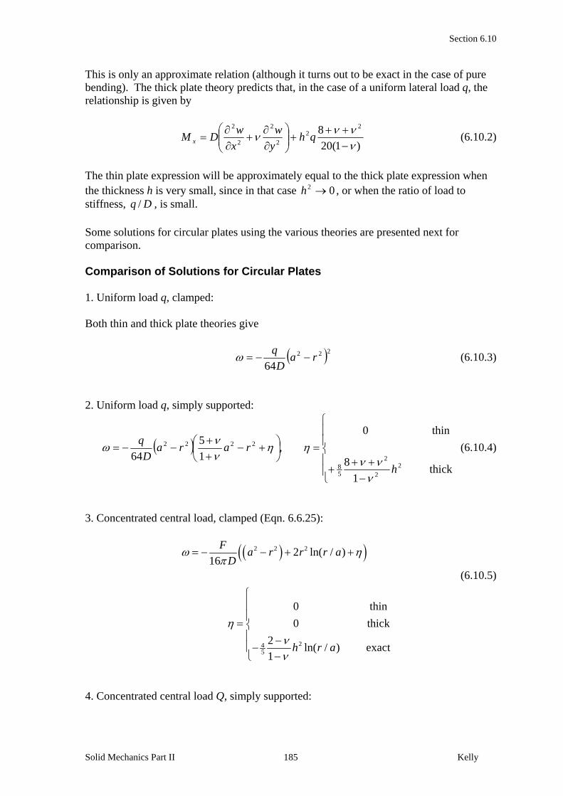
Section 6.10


This is only an approximate relation (although it turns out to be exact in the case of pure bending). The thick plate theory predicts that, in the case of a uniform lateral load q, the relationship is given by

)1(20

8 22

2

2

2

2

qhy

w

x

wDM x (6.10.2)

The thin plate expression will be approximately equal to the thick plate expression when the thickness h is very small, since in that case 02 h , or when the ratio of load to stiffness, Dq / , is small. Some solutions for circular plates using the various theories are presented next for comparison. Comparison of Solutions for Circular Plates 1. Uniform load q, clamped: Both thin and thick plate theories give

222

64ra

D

q (6.10.3)

2. Uniform load q, simply supported:

thick1

8

thin0

,1

5

642

2

2

58

2222

h

raraD

q

(6.10.4)

3. Concentrated central load, clamped (Eqn. 6.6.25):

2 2 2

245

2 ln( / )16

0 thin

0 thick

2ln( / ) exact

1

Fa r r r a

D

h r a

(6.10.5)

4. Concentrated central load Q, simply supported:

Section 6.10


2 2 2

22 22

5 2

22 2 24 1

5 5 2

32 ln( / )

16 1

0 thin

8thick

1

2 2ln( / ) exact

1 1

Fa r r r a

D

ha r

a

hh r a a r

a

(6.10.6)

Higher-order deformation Theories A further theory known as third-order plate theory has also been developed. This allows for the displacements to vary not only linearly (the previously described Mindlin theory is also called the first order shear deformation theory), but as cubic functions; the in-plane strains are cubic ( 3~ z ) and the shear strains are quadratic. This allows the line elements normal to the mid-surface not only to rotate, but also to deform and not necessarily remain straight. 6.10.2 Large Deflections Consider now the assumption that the membrane stresses may be neglected. To investigate the validity of this, consider an initially circular plate of diameter d, clamped at the edges, and deformed into a spherically shaped surface, Fig. 6.10.1.

Figure 6.10.1: a deformed circular plate Considering a beam, the length of the neutral axis before and after deformation can safely be taken to be equal, even when the beam deforms as in Fig. 6.10.1, i.e. one can take

dd . The reason for this is that the “supports” are assumed to move slightly to accommodate any small deflection; thus the neutral axis of a beam remains strain-free and hence stress-free.

d

R

2

d

w

Section 6.10


Consider next the plate. Suppose that the supports could move slightly to accommodate the deformation of the plate so that the curved length in Fig. 6.10.1 was equal in length to the original diameter. One then sees that a compressive circumferential strain is set up in the plate mid-surface, of magnitude ddd / . To quantify this, note that Rd 2/

and Rd 2/sin . Thus !5/2/!3/2/2/2/ 53 RdRdRdRd . Then

220

1920

1

24

1

R

d

R

d (6.10.7)

With Rw /1cos and !2/1cos 2 , one also has

2

42 1

384

1

8

1

R

d

ww

dR (6.10.8)

so that, approximately,

2

20

3

8

d

w (6.10.9)

The maximum bending strain occurs at 2/hz , where )/1)(2/.( Rhrr , so

2

4

d

hwrr (6.10.10)

One can conclude from this rough analysis that, in order that the membrane strains can be safely ignored, the deflection w must be small when compared to the thickness h of the plate1. The corollary of this is that when there are large deflections, the middle surface will strain and take up the load as in a stretching membrane. For the bending of circular plates, one usually requires that hw 5.0 in order that the membrane strains can be safely ignored without introducing considerable error. For example, a uniformly loaded clamped plate deflected to hw experiences a maximum membrane stress of approximately 20% of the maximum bending stress. When the deflections are large, the membrane strains need to be considered. This means that the von Kármán strains, Eqns. 6.2.22, 6.2.25, must be used in the analysis. Further, the in-plane forces, for example in the bending Eqn. 6.7.6, are now an unknown of the problem. Some approximate solutions of the resulting equations have been worked out, for example for uniformly loaded circular and rectangular plates.

1 except in some special cases, for example when a plate deforms into the surface of a cylinder

Documents

6.1 Plate Theory - Auckland