Embed Size (px)
Citation preview
6. Production
Literature:
Pindyck und Rubinfeld, Chapter 6
Varian, Chapter 18

| 23.05.2017 | Prof. Dr. Kerstin Schneider| Chair of Public Economics and Business Taxation | Microeconomics| Chapter 6 Slide 2 |
Chapter Outline
• Production Technology
• Production with One Input Variable (Labor)
• Production with Two Input Variables
• Returns to Scale

| 23.05.2017 | Prof. Dr. Kerstin Schneider| Chair of Public Economics and Business Taxation | Microeconomics| Chapter 6 Slide 3 |
Introduction
• In this chapter, we will focus on the supply side.
• Theory of the firm:
– How does a firm minimize costs or maximize profits with
regard to its production decisions?
– How do costs vary with production?
– Characteristics of market supply.
| 23.05.2017 | Prof. Dr. Kerstin Schneider| Chair of Public Economics and Business Taxation | Microeconomics| Chapter 6 Slide 4 |
The Technology of Production
• The production process
– The combination of inputs or production factors required
to produce a certain level of output.
• Factors of Production
– Labor
– Material
– Capital

| 23.05.2017 | Prof. Dr. Kerstin Schneider| Chair of Public Economics and Business Taxation | Microeconomics| Chapter 6 Slide 5 |
The Technology of Production
• The Production function
– Function showing the highest output that a firm can
produce for each specified combination of inputs.
– Describes what is technically feasible when the firm
operates efficiently, i.e., when the firm uses each
combination of inputs as efficiently as possible.

| 23.05.2017 | Prof. Dr. Kerstin Schneider| Chair of Public Economics and Business Taxation | Microeconomics| Chapter 6 Slide 6 |
The Technology of Production
• A production function with a given technology of two inputs
is as follows:
Q = F(K,L)
Q = Output, K = Capital, L = Labor
| 23.05.2017 | Prof. Dr. Kerstin Schneider| Chair of Public Economics and Business Taxation | Microeconomics| Chapter 6 Slide 7 |
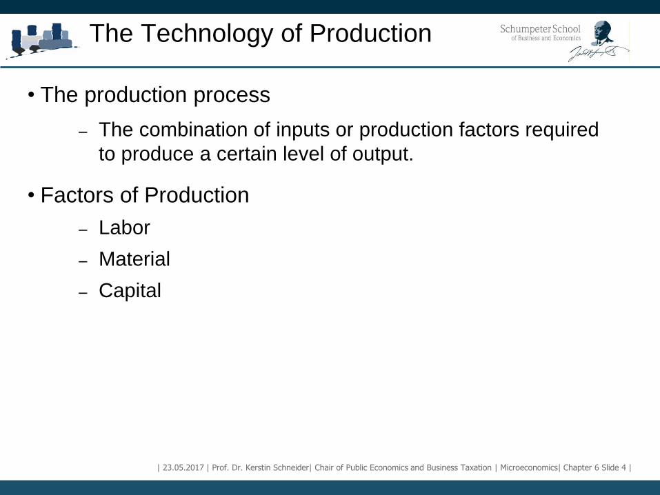
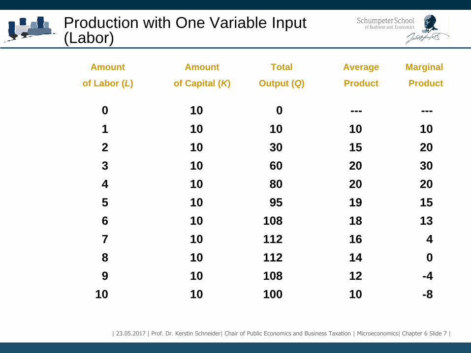
Production with One Variable Input (Labor)
Amount Amount Total Average Marginal
of Labor (L) of Capital (K) Output (Q) Product Product
0 10 0 --- ---
1 10 10 10 10
2 10 30 15 20
3 10 60 20 30
4 10 80 20 20
5 10 95 19 15
6 10 108 18 13
7 10 112 16 4
8 10 112 14 0
9 10 108 12 -4
10 10 100 10 -8
| 23.05.2017 | Prof. Dr. Kerstin Schneider| Chair of Public Economics and Business Taxation | Microeconomics| Chapter 6 Slide 8 |
Production with One Variable Input (Labor)
• Note that
1) with each additional unit of labor, the quantity (Q)
produced increases, reaches a maximum, and then
decreases.

| 23.05.2017 | Prof. Dr. Kerstin Schneider| Chair of Public Economics and Business Taxation | Microeconomics| Chapter 6 Slide 9 |
Production with One Variable Input (Labor)
• Note that
2) The average product of labor ( ), initially
increases with each additional unit of labor until
reaching a global maximum after which it decreases
with each additional unit of labor.
L
Output QAP
Labor input L
LAP
| 23.05.2017 | Prof. Dr. Kerstin Schneider| Chair of Public Economics and Business Taxation | Microeconomics| Chapter 6 Slide 10 |
Production with One Variable Input (Labor)
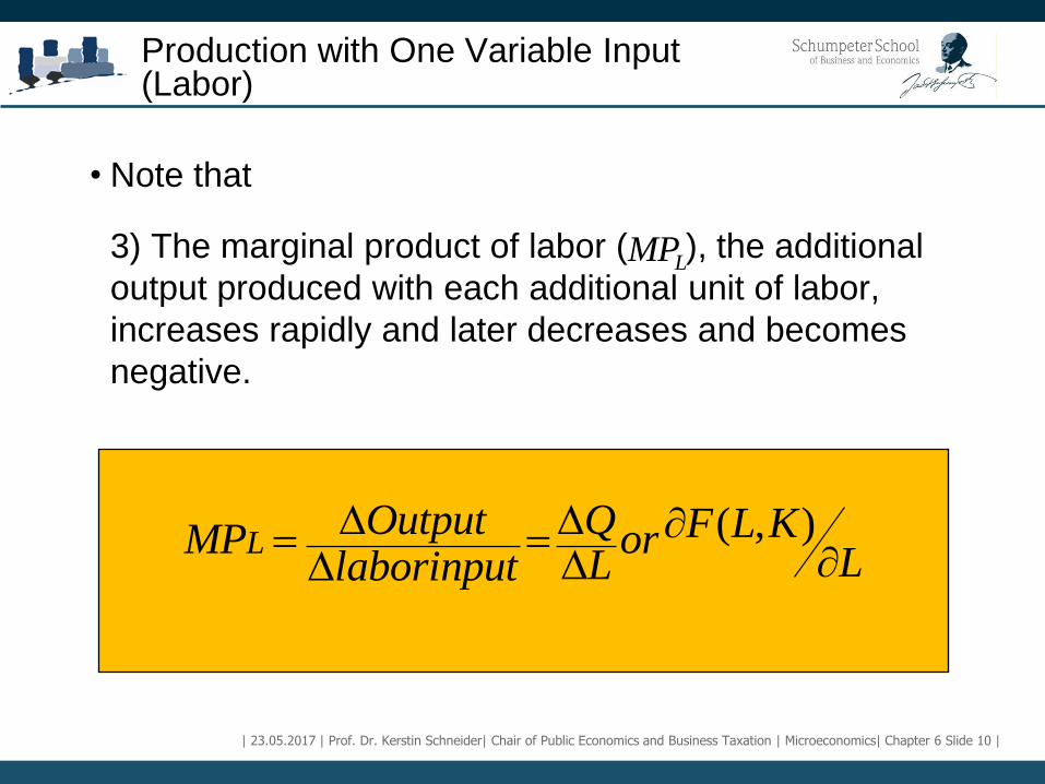
• Note that
3) The marginal product of labor ( ), the additional
output produced with each additional unit of labor,
increases rapidly and later decreases and becomes
negative.
( , )L
Output Q F L KMP orLLlaborinput
LMP

| 23.05.2017 | Prof. Dr. Kerstin Schneider| Chair of Public Economics and Business Taxation | Microeconomics| Chapter 6 Slide 11 |
Production with One Variable Input (Labor)
Total Product
A: tangent to the total product
curve with slope = MP (20)
B: slope of 0B = AP (20)
C: slope of 0C= MP & AP
Labor per month
Output
per
month
60
112
0 2 3 4 5 6 7 8 9 10 1
A
B
C
D
| 23.05.2017 | Prof. Dr. Kerstin Schneider| Chair of Public Economics and Business Taxation | Microeconomics| Chapter 6 Slide 12 |
Production with One Variable Input (Labor)
Average Product
8
10
20
Output
per
month
0 2 3 4 5 6 7 9 10 1
30
E
Marginal Product
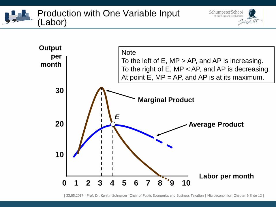
Note
To the left of E, MP > AP, and AP is increasing.
To the right of E, MP < AP, and AP is decreasing.
At point E, MP = AP, and AP is at its maximum.
Labor per month
| 23.05.2017 | Prof. Dr. Kerstin Schneider| Chair of Public Economics and Business Taxation | Microeconomics| Chapter 6 Slide 13 |
Production with One Variable Input (Labor)
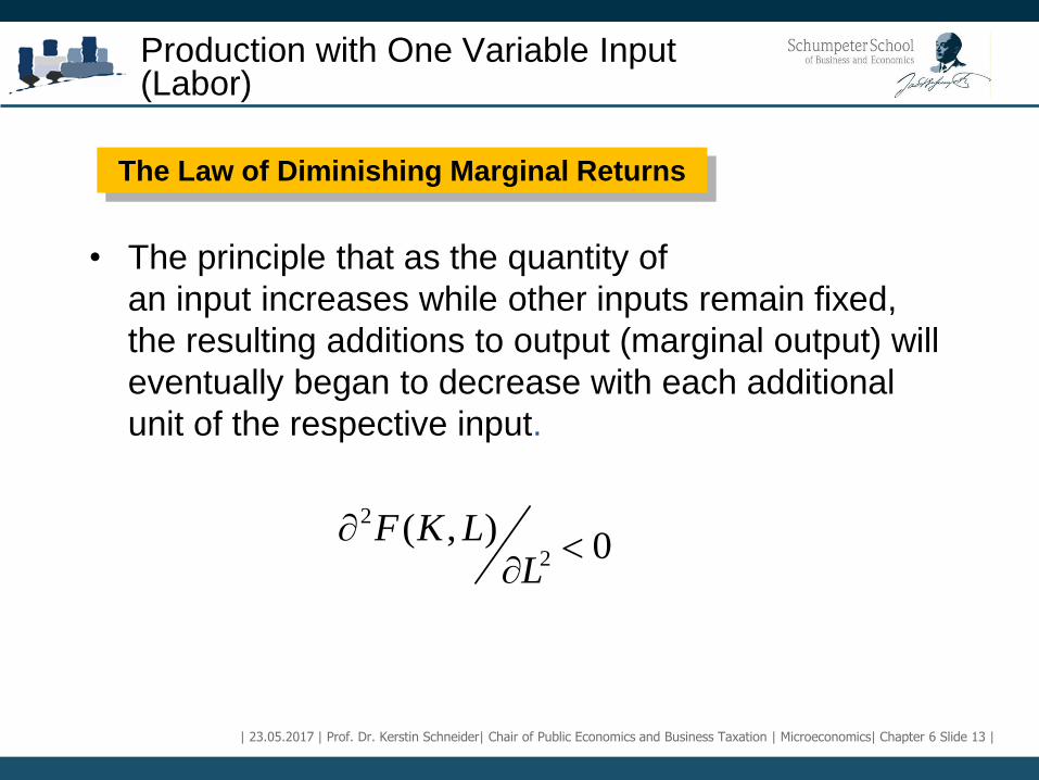
• The principle that as the quantity of
an input increases while other inputs remain fixed,
the resulting additions to output (marginal output) will
eventually began to decrease with each additional
unit of the respective input.
The Law of Diminishing Marginal Returns
2
2
( , )0
F K LL
| 23.05.2017 | Prof. Dr. Kerstin Schneider| Chair of Public Economics and Business Taxation | Microeconomics| Chapter 6 Slide 14 |
Production with One Variable Input (Labor)
• If labor input is low, MP increases due to
specialization.
• If labor input is high, MP decreases due to inefficiency.
The Law of Diminishing Marginal Returns

| 23.05.2017 | Prof. Dr. Kerstin Schneider| Chair of Public Economics and Business Taxation | Microeconomics| Chapter 6 Slide 15 |
The Effect of Technological Improvement
Labor per time period
Output per time
period
50
100
0 2 3 4 5 6 7 8 9 10 1
A
O1
C
O3
O2
B
Even though any given
production process
exhibits diminishing
returns to labor,
labor productivity
(output per unit of labor)
can increase if there
are improvements in
technology.

| 23.05.2017 | Prof. Dr. Kerstin Schneider| Chair of Public Economics and Business Taxation | Microeconomics| Chapter 6 Slide 16 |
Malthus and the food crisis
• Malthus predicted that as both the marginal and average
productivity of labor fell and there were more mouths to
feed, mass hunger and starvation would result.
• Why was Malthus’ prediction wrong?

| 23.05.2017 | Prof. Dr. Kerstin Schneider| Chair of Public Economics and Business Taxation | Microeconomics| Chapter 6 Slide 17 |
Index of World Food Production per Capita
1948-1952 100
1960 115
1970 123
1980 128
1990 138
1995 140
2001 161
Year Index

| 23.05.2017 | Prof. Dr. Kerstin Schneider| Chair of Public Economics and Business Taxation | Microeconomics| Chapter 6 Slide 18 |
Malthus and the food crisis
• The data shows that increases in production exceeded population growth.
• Malthus did not take technological improvements into account.
• Over the past century, technological improvements have dramatically altered food production in most countries (including developing countries, e.g., India).
• As a result, the average product of labor and total food
production have increased.
• Therefore, technological improvements can create
surpluses and reduce prices.

| 23.05.2017 | Prof. Dr. Kerstin Schneider| Chair of Public Economics and Business Taxation | Microeconomics| Chapter 6 Slide 19 |
Malthus and the food crisis
• Question:
– Why does hunger remain a severe problem in some areas
of the world?

| 23.05.2017 | Prof. Dr. Kerstin Schneider| Chair of Public Economics and Business Taxation | Microeconomics| Chapter 6 Slide 20 |
Production with One Variable Input (Labor)
• Labor Productivity
total outputAverage Productivity
total labor input

| 23.05.2017 | Prof. Dr. Kerstin Schneider| Chair of Public Economics and Business Taxation | Microeconomics| Chapter 6 Slide 21 |
Production with One Variable Input (Labor)
• Productivity and the standard of living
– Consumers—in the aggregate—can only increase their
rate of consumption in the long run by increasing the total
amount they produce. Understanding the causes of
productivity growth is an important area of research in
economics.
– Determinants of productivity of labor
Stock of capital
Technological change
| 23.05.2017 | Prof. Dr. Kerstin Schneider| Chair of Public Economics and Business Taxation | Microeconomics| Chapter 6 Slide 22 |
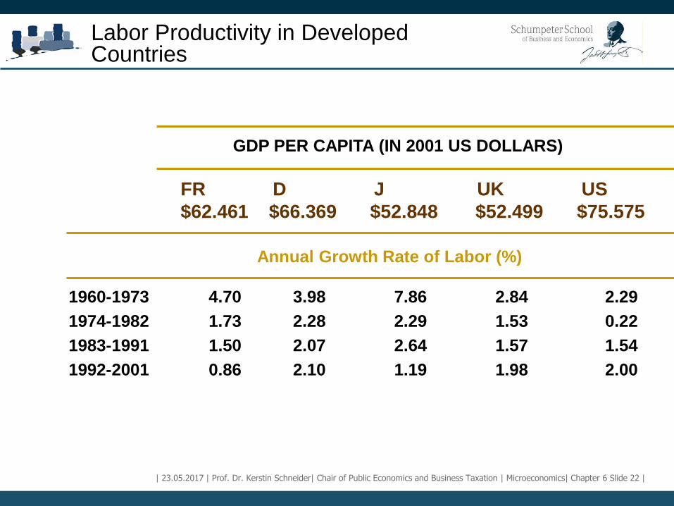
Labor Productivity in Developed Countries
1960-1973 4.70 3.98 7.86 2.84 2.29
1974-1982 1.73 2.28 2.29 1.53 0.22
1983-1991 1.50 2.07 2.64 1.57 1.54
1992-2001 0.86 2.10 1.19 1.98 2.00
Annual Growth Rate of Labor (%)
FR D J UK US
$62.461 $66.369 $52.848 $52.499 $75.575
GDP PER CAPITA (IN 2001 US DOLLARS)
| 23.05.2017 | Prof. Dr. Kerstin Schneider| Chair of Public Economics and Business Taxation | Microeconomics| Chapter 6 Slide 23 |
Production with Two Variable Inputs
• There is a relationship between production and
productivity.
• Both labor and capital are variable in the long run.
• Analyze isoquants and compare the different combinations
of K & L and the respective quantities produced.
• Do you see similarities to indifference curves?
| 23.05.2017 | Prof. Dr. Kerstin Schneider| Chair of Public Economics and Business Taxation | Microeconomics| Chapter 6 Slide 24 |
The Isoquants
• Isoquants show the flexibility that firms have when
making production decisions: they can usually obtain a
particular output by substituting one input for another.
• This information allows the producer to react
effectively to market changes for inputs, e.g., changes
in price, quality, and availability.
Input flexibility

| 23.05.2017 | Prof. Dr. Kerstin Schneider| Chair of Public Economics and Business Taxation | Microeconomics| Chapter 6 Slide 25 |
The Isoquants
• Short run:
• Short-run production refers to production that can
be completed when at least one factor of
production is fixed.
• These inputs are called fixed production factors.
• Long run:
– A period of time in which all factors of production and
costs are variable.
The Short and the Long Run

| 23.05.2017 | Prof. Dr. Kerstin Schneider| Chair of Public Economics and Business Taxation | Microeconomics| Chapter 6 Slide 26 |
Production with Two Input Variables (L, k)
Labor per year
1
2
3
4
1 2 3 4 5
5
Q1 = 55
The isoquants are derived from the
production function for a quantity
produced of 55, 75, and 90,
respectively.
A
D
B
Q2 = 75
Q3 = 90
C
E
Capital
per year Isoquants
| 23.05.2017 | Prof. Dr. Kerstin Schneider| Chair of Public Economics and Business Taxation | Microeconomics| Chapter 6 Slide 27 |
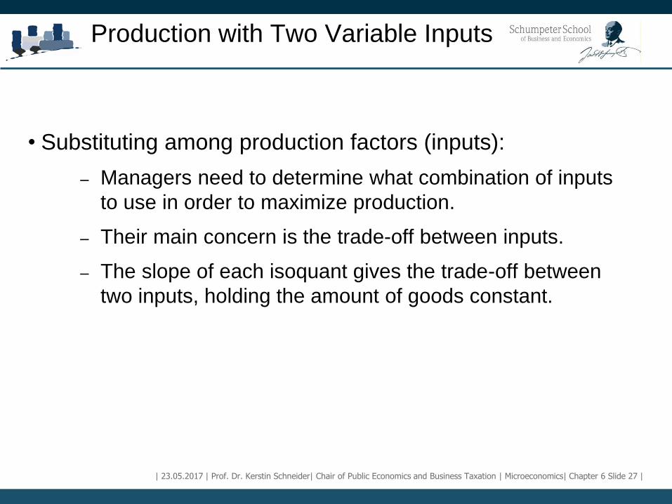
Production with Two Variable Inputs
• Substituting among production factors (inputs):
– Managers need to determine what combination of inputs
to use in order to maximize production.
– Their main concern is the trade-off between inputs.
– The slope of each isoquant gives the trade-off between
two inputs, holding the amount of goods constant.

| 23.05.2017 | Prof. Dr. Kerstin Schneider| Chair of Public Economics and Business Taxation | Microeconomics| Chapter 6 Slide 28 |
Production with Two Variable Inputs
Substituting among production factors (inputs):
– The marginal rate of technical substitution (MRTS):
Ä /Änderung des ArbeitskräfteeinesatzesGRTS - nderung des Kapitaleinsatzes
(for a fixed level )
or
KMRTS QL
dKMRTSdL
| 23.05.2017 | Prof. Dr. Kerstin Schneider| Chair of Public Economics and Business Taxation | Microeconomics| Chapter 6 Slide 29 |
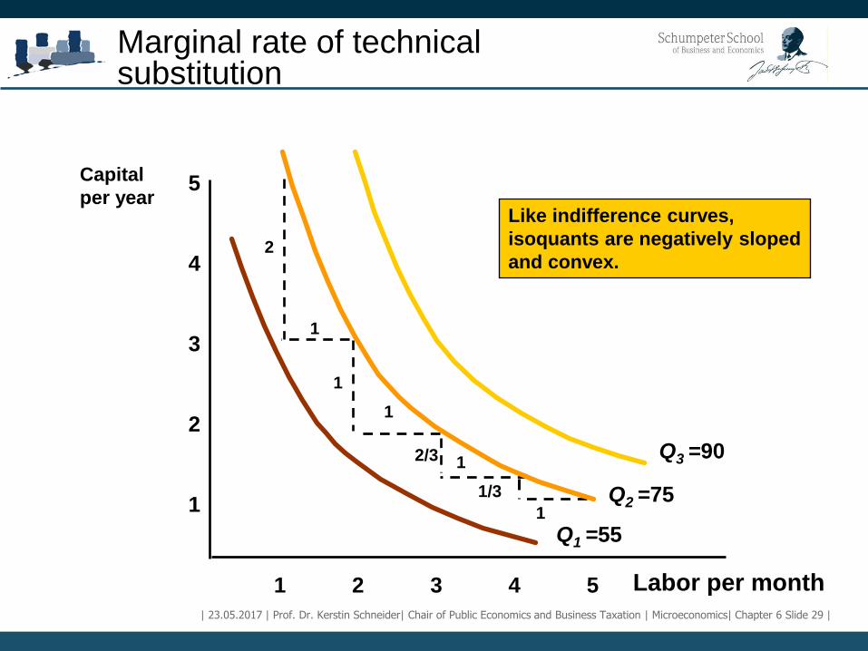
Marginal rate of technical substitution
Labor per month
1
2
3
4
1 2 3 4 5
5 Capital
per year Like indifference curves,
isoquants are negatively sloped
and convex.
1
1
1
1
2
1
2/3
1/3
Q1 =55
Q2 =75
Q3 =90

| 23.05.2017 | Prof. Dr. Kerstin Schneider| Chair of Public Economics and Business Taxation | Microeconomics| Chapter 6 Slide 30 |
Production with Two Input Variables
1) Increasing labor from 1 to 5 leads to a decrease in MRTS from 2 to 1/3.
2) The diminishing MRTS occurs due to decreasing marginal returns, which implies that isoquants are convex.
3) The MRTS and the marginal product
The result of a change in labor resulting from a
change in the quantity of goods is equal to
L(MP )( L)

| 23.05.2017 | Prof. Dr. Kerstin Schneider| Chair of Public Economics and Business Taxation | Microeconomics| Chapter 6 Slide 31 |
Production with Two Input Variables
• Note:
3) The MRTS and the marginal product
• The result of a change in the quantity of
goods resulting from a change in the quantity
of capital is equal to
K(MP )( K)

| 23.05.2017 | Prof. Dr. Kerstin Schneider| Chair of Public Economics and Business Taxation | Microeconomics| Chapter 6 Slide 32 |
Production with Two Input Variables
• Note:
3) The MRTS and the marginal product
If quantity is fixed ( ) and labor input
increases, then
L K(MP )( L) (MP )( K) 0
L K(MP ) / (MP ) - ( K / L) MRTS
0Q
| 23.05.2017 | Prof. Dr. Kerstin Schneider| Chair of Public Economics and Business Taxation | Microeconomics| Chapter 6 Slide 33 |
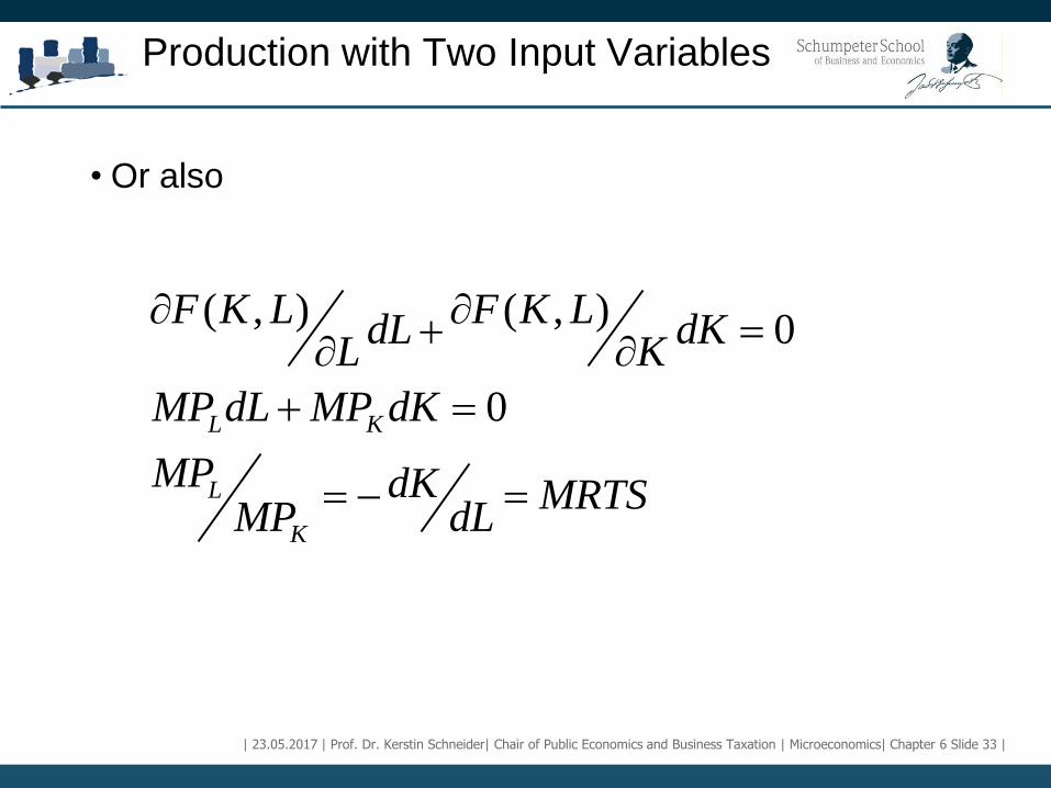
Production with Two Input Variables
• Or also
( , ) ( , )0
0L K
L
K
F K L F K LdL dK
L K
MP dL MP dK
MP dK MRTSMP dL
| 23.05.2017 | Prof. Dr. Kerstin Schneider| Chair of Public Economics and Business Taxation | Microeconomics| Chapter 6 Slide 34 |
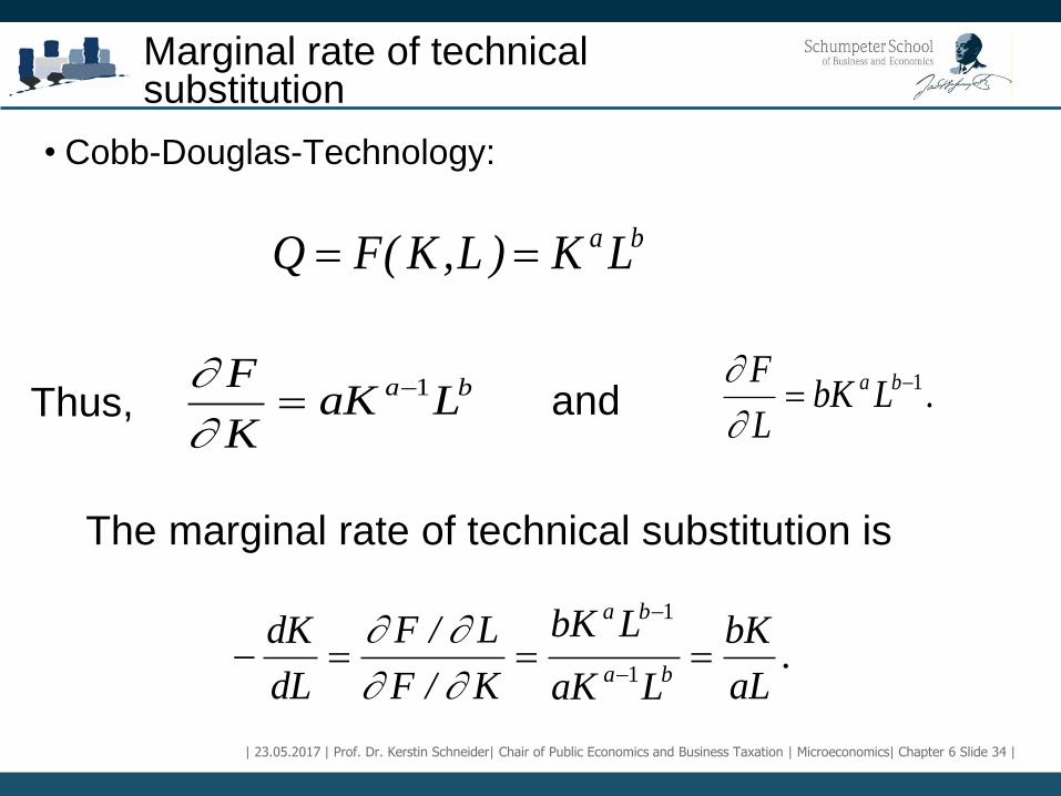
Marginal rate of technical substitution
• Cobb-Douglas-Technology:
ba LK)L,K(FQ
Thus, ba LaK
K
F 1
.LbK
L
F ba 1
and
The marginal rate of technical substitution is
.aL
bK
LaK
LbK
K/F
L/F
dL
dKba
ba
1
1
| 23.05.2017 | Prof. Dr. Kerstin Schneider| Chair of Public Economics and Business Taxation | Microeconomics| Chapter 6 Slide 35 |
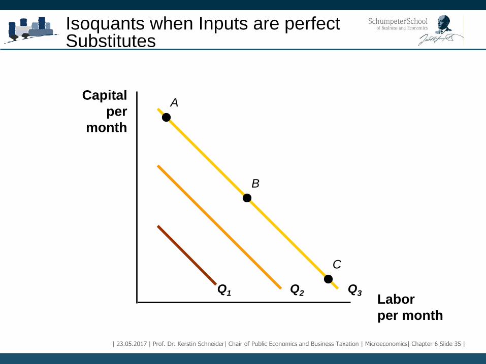
Isoquants when Inputs are perfect Substitutes
Labor
per month
Capital
per
month
Q1 Q2 Q3
A
B
C
| 23.05.2017 | Prof. Dr. Kerstin Schneider| Chair of Public Economics and Business Taxation | Microeconomics| Chapter 6 Slide 36 |
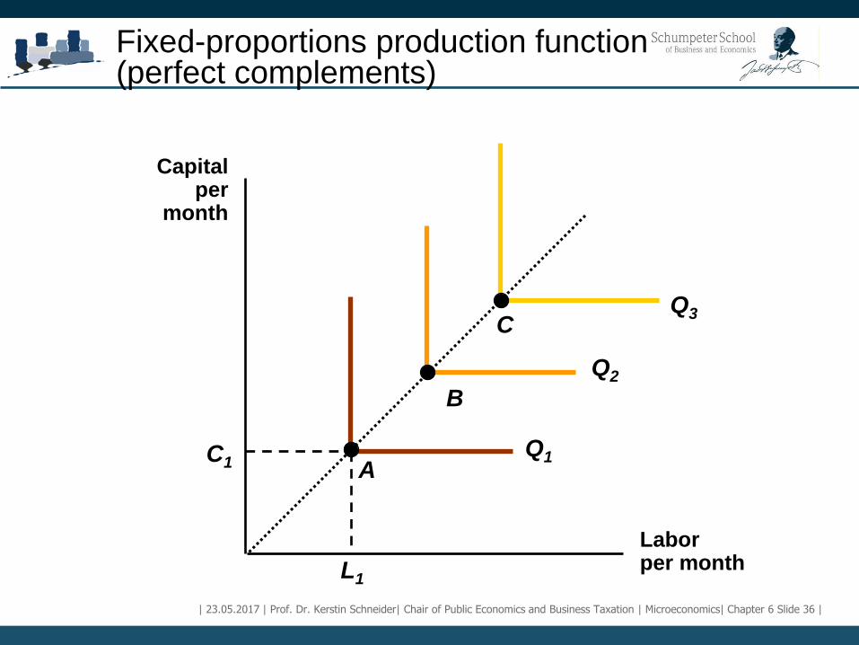
Fixed-proportions production function (perfect complements)
Labor per month
Capital per
month
L1
C1 Q1
Q2
Q3
A
B
C

| 23.05.2017 | Prof. Dr. Kerstin Schneider| Chair of Public Economics and Business Taxation | Microeconomics| Chapter 6 Slide 37 |
Example: A Production Function for Wheat
• Farmers must choose between a capital-intensive and
labor-intensive production function.

| 23.05.2017 | Prof. Dr. Kerstin Schneider| Chair of Public Economics and Business Taxation | Microeconomics| Chapter 6 Slide 38 |
Isoquants describing the Production of Wheat
Labor
(hours per year)
Capital
(machine
hours per
year)
250 500 760 1000
40
80
120
100
90
Output = 13,800 Bushels
per year
A
B 10- K
260 L
Point A is more capital-intensive.
Point B is more labor-intensive.
| 23.05.2017 | Prof. Dr. Kerstin Schneider| Chair of Public Economics and Business Taxation | Microeconomics| Chapter 6 Slide 39 |
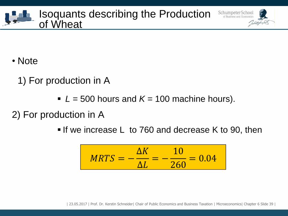
Isoquants describing the Production of Wheat
• Note
1) For production in A
L = 500 hours and K = 100 machine hours).
2) For production in A
If we increase L to 760 and decrease K to 90, then
𝑀𝑅𝑇𝑆 = −
Δ𝐾
Δ𝐿= −
10
260= 0.04

| 23.05.2017 | Prof. Dr. Kerstin Schneider| Chair of Public Economics and Business Taxation | Microeconomics| Chapter 6 Slide 40 |
Isoquants describing the Production of Wheat
• Note
3) MRTS < 1, this means that the cost for labor is less than that of capital, otherwise we would have replaced labor with capital.
4) If labor is costly, then the farmer will substitute labor for more capital (e.g., in the USA).
5) If labor is cheap, then the farmer will substitute his capital for more labor (e.g., in India).
| 23.05.2017 | Prof. Dr. Kerstin Schneider| Chair of Public Economics and Business Taxation | Microeconomics| Chapter 6 Slide 41 |
Returns to Scale
• Returns to scale: rate at which output increases as inputs
increase proportionately.
1) Increasing returns to scale: situation in which output
more than doubles when all inputs are doubled.
A larger quantity of goods is associated with lower
costs (cars).
One company is more efficient than many companies
(public utilities).
The distance between the isoquants becomes
smaller.

| 23.05.2017 | Prof. Dr. Kerstin Schneider| Chair of Public Economics and Business Taxation | Microeconomics| Chapter 6 Slide 42 |
Returns to Scale
Labor (hours)
Capital
(machine
hours)
10
20
30
Increasing returns to scale: the
isoquants move closer together as
inputs increase along line A.
5 10
2
4
0
A

| 23.05.2017 | Prof. Dr. Kerstin Schneider| Chair of Public Economics and Business Taxation | Microeconomics| Chapter 6 Slide 43 |
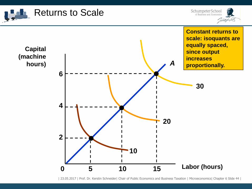
Returns to Scale
2) Constant returns to scale: Situation in which output doubles when all inputs are doubled.
Size does not affect productivity.
There may be a large number of producers.
The distance between the isoquants is constant.
| 23.05.2017 | Prof. Dr. Kerstin Schneider| Chair of Public Economics and Business Taxation | Microeconomics| Chapter 6 Slide 44 |
Returns to Scale
Labor (hours)
Capital
(machine
hours)
Constant returns to
scale: isoquants are
equally spaced,
since output
increases
proportionally.
10
20
30
15 5 10
2
4
0
A
6
| 23.05.2017 | Prof. Dr. Kerstin Schneider| Chair of Public Economics and Business Taxation | Microeconomics| Chapter 6 Slide 45 |
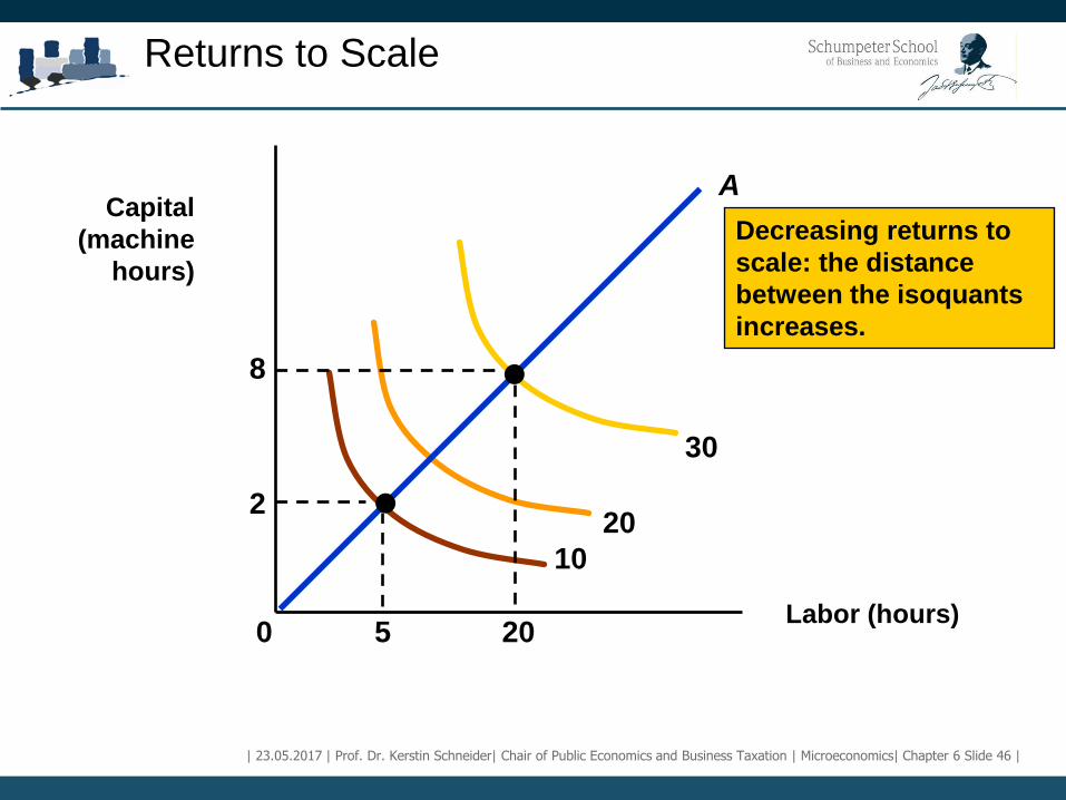
Returns to Scale
3) Decreasing returns to scale: Situation in which output less than doubles when all inputs are doubled.
Efficiency decreases as size increases.
Reduces the firm’s production abilities.
The distance between the isoquants increases.
| 23.05.2017 | Prof. Dr. Kerstin Schneider| Chair of Public Economics and Business Taxation | Microeconomics| Chapter 6 Slide 46 |
Returns to Scale
Labor (hours)
Capital
(machine
hours)
Decreasing returns to
scale: the distance
between the isoquants
increases.
10
20
30
5 20
2
8
0
A
| 23.05.2017 | Prof. Dr. Kerstin Schneider| Chair of Public Economics and Business Taxation | Microeconomics| Chapter 6 Slide 47 |
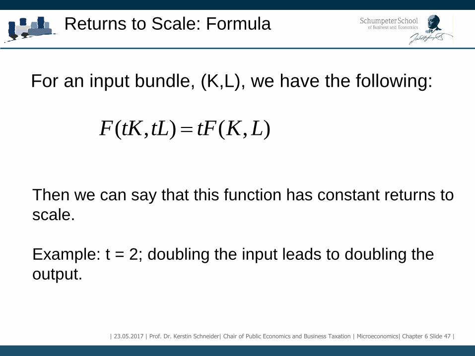
Returns to Scale: Formula
For an input bundle, (K,L), we have the following:
( , ) ( , )F tK tL tF K L
Then we can say that this function has constant returns to
scale.
Example: t = 2; doubling the input leads to doubling the
output.

| 23.05.2017 | Prof. Dr. Kerstin Schneider| Chair of Public Economics and Business Taxation | Microeconomics| Chapter 6 Slide 48 |
Returns to Scale: Formula
For an input bundle, (K,L), we have the following:
( , ) ( , )F tK tL tF K L
We can say that this function has increasing returns to
scale.
Example: t = 2; doubling the input leads to more than double
the output.
| 23.05.2017 | Prof. Dr. Kerstin Schneider| Chair of Public Economics and Business Taxation | Microeconomics| Chapter 6 Slide 49 |
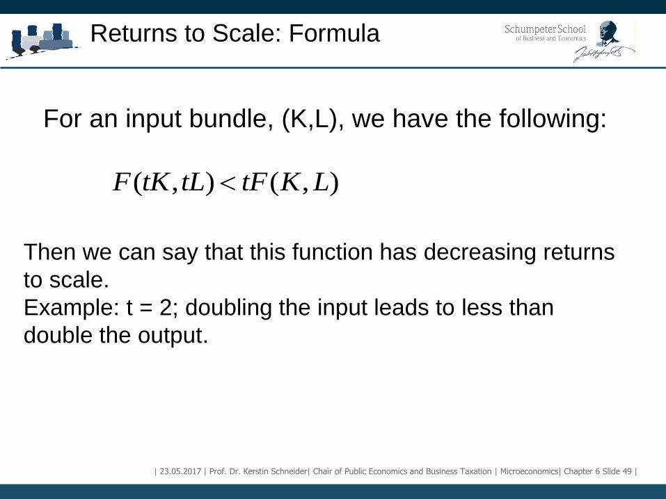
Returns to Scale: Formula
For an input bundle, (K,L), we have the following:
( , ) ( , )F tK tL tF K L
Then we can say that this function has decreasing returns
to scale.
Example: t = 2; doubling the input leads to less than
double the output.
| 23.05.2017 | Prof. Dr. Kerstin Schneider| Chair of Public Economics and Business Taxation | Microeconomics| Chapter 6 Slide 50 |
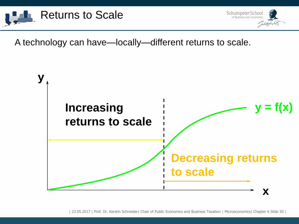
Returns to Scale
y = f(x)
x
y
Decreasing returns
to scale
Increasing
returns to scale
A technology can have—locally—different returns to scale.
| 23.05.2017 | Prof. Dr. Kerstin Schneider| Chair of Public Economics and Business Taxation | Microeconomics| Chapter 6 Slide 51 |
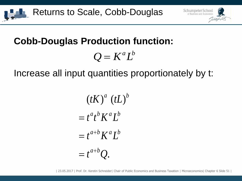
Returns to Scale, Cobb-Douglas
a bQ K L
Cobb-Douglas Production function:
Increase all input quantities proportionately by t:
( ) ( )
.
a b
a b a b
a b a b
a b
tK tL
t t K L
t K L
t Q
| 23.05.2017 | Prof. Dr. Kerstin Schneider| Chair of Public Economics and Business Taxation | Microeconomics| Chapter 6 Slide 52 |
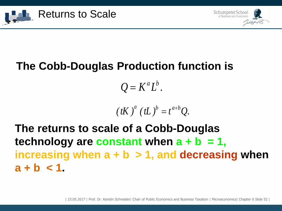
Returns to Scale
The Cobb-Douglas Production function is
.LKQ ba
.Qt)tL()tK( baba
The returns to scale of a Cobb-Douglas
technology are constant when a + b = 1,
increasing when a + b > 1, and decreasing when
a + b < 1.
| 23.05.2017 | Prof. Dr. Kerstin Schneider| Chair of Public Economics and Business Taxation | Microeconomics| Chapter 6 Slide 53 |
Concluding Remarks
• A production function describes the maximum output that a
company can produce given any particular input
combination.
• An isoquant is a curve representing all input combinations
with which a given level of output can be achieved.
| 23.05.2017 | Prof. Dr. Kerstin Schneider| Chair of Public Economics and Business Taxation | Microeconomics| Chapter 6 Slide 54 |
Concluding Remarks
• The average product of labor measures the productivity of
the average unit of labor, whereas the laborer's marginal
product measures the productivity of the last added unit of
labor.
• The law of decreasing marginal returns states that the
marginal product of an input ultimately decreases as its
quantity increases, ceteris paribus.
• Isoquants are always negatively sloped, because the
marginal product of all inputs is positive.