6 Estimation - fairmodel.econ.yale.edu

6 Estimation

6.1 Introduction

Macroeconometric models are typically nonlinear, simultaneous, and large. They also tend to have error terms that are serially correlated. The focus of this chapter is on models with these characteristics. The notation that will be used in this chapter and in Chapters 7- 10 is as follows. Write the model as

(6.1) f;(Y,, &, 4 = 4, i= 1, ,n, t=1,. ,r,

where y, is an ndimensional vector of endogenous variables, x, is a vector of predetermined variables, q is a vector of unknown coefficients, and ui, is an error term. Assume that the first m equations are stochastic, with the remaining ui, (i = m + 1, , n) identically zero for all 1.

Let J, be the n X n Jacobian matrix whose ij element is ah;layjAi, j= 1, , n). Also, let u, be the T-dimensional vector (ui,, , uir)‘, and let u be the m . T-dimensional vector (u I,, , U,T. > %d, , %A’. Let a denote the k-dimensional vector (01;) , 01;) of all the unknown coefficients. Finally, let G;be the k, X Tmatrix whose tth column is al(_v,, x,, ai)/&xi, where ki is the dimension of q, and let G’ be the k X m . Tmatrix,

G; 0 . . 0 0 G;

1: 0 ..( 1 G:.

where k = ZZc I ki. These vectors and matrices will be used in the following sections.

6.2 Treatment of Serial Correlation

A convenient way ofdealing with serially correlated error terms is to treat the serial correlation coefficients as structural coefficients and to transform the

210 Macroeconometric Models

Since many equations in macroeconometric models have lagged dependent variables, the DW test is of limited use. My response to this problem is to estimate the equations initially under the assumption of serial correlation (usually first-order) by some consistent technique (usually 2SLS). From this, one can test the hypothesis that the serial correlation coefficients are zero, which is simply a &test on each coefficient. This test is valid asymptotically if one has correctly estimated the asymptotic covariance matrix ofthe estimated coefficients, and it is not restricted to equations without lagged dependent variables. It also easily handles serial correlation of higher than first order. since all this requires is estimating the equation under the assumption ofthe particular order. If a test indicates that a serial correlation coefficient is zero, the equation can be reestimated without this coefficient being included.

Although this is the general procedure that I follow in handling serial correlation problems, I still include the DW statistic in the presentation ofthe results for a particular equation (see Chapter 4). Since the DW statistic is biased toward acceptance of the hypothesis of no serial correlation when there are lagged dependent variables, a value that rejects the hypothesis indicates that there are likely to be problems. The DW test is thus useful for testing in one direction, and this is the reason I tend to include it in the results.

6.3 Estimation Techniques

6.3.1 Ordinary Least Squares (OLS)

The OLS technique is a special case of the 2SLS technique, where 0, in (6.5) and (6.6) below is the identity matrix. It is thus unnecessary to consider this technique separately from the 2SLS technique.

6.3.2 Two-Stage Least Squares (2SLS)

Generul Case

2SLS estimates of LY, (say &J are obtained by minimizing

(6.5) u~z,(z~z,)-‘z~ui = &DiUi

with respect to cxi, where Z, is a TX K, matrix of predetermined variables. Zi and K, can differ from equation to equation. An estimate of the covariance matrix of @ (sap Pz;,) is

(6.6) P2i; = i?,,(i;:&~i)-~,

where 6, is Gi evaluated at&and ?Jij = T-l EL, Lit, a, =f;(r,, x,, &J.

Estimation 211

The 2SLS estimator in this form is presented in Amemiya (1974). It handles the case of nonlinearity in both variables and coefficients. In earlier work, Kelejian ( 197 I) considered the case of nonlinearity in variables only. Bierens ( I98 1, p. 106) has pointed out that Amemiya’s proofofconsistency of this estimator is valid only in the case of linearity in the coefficients, that is, only in Kelejian’s case. Bierens supplies a proof of consistency and asymptotic normality in the general case.

It will be useful to consider the special case in which the equation to be estimated is linear in coefficients. Write equation i in this case as

(6.7) y,=x;oli+u,,

where y,is the T-dimensional vector&, , yir)‘and X,isa TX kimatrix of observations on the explanatory variables in the equation. Xi includes both endogenous and predetermined variables. Both y, and the variables in X, can be nonlinear functions of other variables, and thus (6.7) is much more general than the standard linear model. All that is required is that the equation be linear in 01,. Substituting ui = J+ - X,(Y~ into (6.5), differentiating with respect to cu,, and setting the derivatives equal to zero yields the following formula for &i:

(6.8) & = (X:D,X,)-‘x;D,y, = (~:XJ-l‘&

where ,?i = QX, is the matrix of predicted values ofthe regression ofX, on 2,. Since 0: = Di and &Di = Di, ,%?$; = ,?;D&X, = $D,X, = *Xi, and thus (6.8) can be written

(6.9) & = (&Q’&,:

which is the standard 2SLS formula in the linear-in-coefficients case. In this case G; is simply Xi, and the formula (6.6) for pzii reduces to

(6. IO) P*ii = CFii($~i)-I.

Linear-in-Coe$icirnts Case wilh Serial Correlarion

It will also be useful to consider the linear-in-coefficients case with serially correlated errors. Assume that ui in (6.7) is first-order serially correlated:

(6. I 1) ui = “i_Ipi + Ei,

212 MacrOeconometric Models

Transforming (6.7) in the manner discussed above yields

(6.12) yi - yi-rpi = (Xi - Xi-,Q.Yi + Ei.

Minimizing e;Diei with respect to oi and pi results in the following first-order conditions:

(6.13) Gi = [_)‘(Xi - X,_,;J-r(~)‘(, - y,-,&),

(6.14) di= (Pi_, -/?-,&i)~(yi-Xi~i)

(Pi-r - J?i_,&J’(.!J_, -X,-,&J ’

where ai = Q(X, - Xi_&, pi_, = DJJ;_ , , and Xi,_, = DJ-, If Xi_, is included in Z,, then 2i_, = Xi_, (since Xi_, is merely the predicted values from a regression of Xi_, on itself and other variables), and therefore X,-X,_,& = Xi - Xi_,ji. If in addition y,_i is included in Z,, then J$_, = yi_, , and (6.14) becomes

“I ^ (6.14)’ ;i = &;:, >

where ai_, = yi_, - A’_,&i and iii = yi -Xi&,. This is merely the fortnula for the coefficient estimate of the regression of r& on (I_,

Equations (6.13) and (6.14) can easily be solved iteratively. Given an initial guess for ji, hi can be computed from (6. I3), and then given &, )i can be computed from (6.14). Given this new value ofji, a new value of bi can be computed from (6.13), and so on. If convergence is reached, which means that the values of hi andfii on successive iterations are within some prescribed tolerance level, the first-order conditions have been solved.

Equations with RHS endogenous variables and serially correlated errors (that is, Eqs. 6.7 and 6.1 I) occur frequently in practice, and the 2SLS estitnator for this case has been widely used. This estimator was discussed in Fair (1970), and I programmed it into the TSP regression package in 1968 under the name TSCORC. (“CORC” refers to the fact that the iterative procedure used to solve Eqs. 6.13 and 6. I4 is like the Cochrane-Orcutt [ 19491 iterative procedure in the nonsimultaneous equations case.) There is an important difference between (6.13) and the formula for sLi proposed in Fair ( 1970), and given the widespread use of the TSCORC command, this difference should be noted. Let Xi= (Y, X,J, where Yi is the matrix of RHS endogenous variables in ($7) and Xii is the matrix of predetermined variables. Let pi = DiYi and X, = (Y? X,J. The formula proposed for &; was

(6.13)’ iuj = [($ - x,_,j+)+i - xi_,fii)]-r(,?i - Xi_,F,)‘(Y, - y-,JJ.

Estimation 213

This is the formula for the coefficient estimates of the regression of yi - JJ+. ,,& on 2i - Xi_,jj. Equation (6.13) reduces to (6.13)’ when &andXi_, =( Yi-, X2,_,) are included in Z,, that is, when the exogenous, lagged endogenous, and lagged exogenous variables in the equation being estimated sre included among the first-stage regressors. The inclusion ofXzi means that yL =fi, and, as noted earlier, the inclusion ofX,_, means that Xi - Xi_,ji = Xi - Xi-,ji. The proposed formula for;< was (6.14)‘, which, as noted above, is the same as (6.14) only ifX+, and yi_, are included in Z,. Solving (6.13)’ and (6.14)’ is thus not the same as solving (6.13) and (6.14) unless X,i, Xi_, , and y,-, are included in Zi. It can be shown that if this is not done, solving (6.13)’ and (6.14)’ does not result in consistent estimates. The need to include X,;, Xi-, , and y,_, among the first-stage regressors was stressed in Fair (1970), but one should keep in mind that this is not absolutely necessary ifthe formulas (6.13) and (6.14) are used. In general, however, Xzi, Xi-, , and y,-, are obvious variables to include among the first-stage regressors, and for most problems this should probably be done even if one is using a program that solves (6.13) and (6.14) rather than (6.13)’ and (6.14)‘.

In the case of linearity in the coefficients and first-order serial correlation, G, = (Xi - X,_,p, yi_l - X+,cu,), and the formula (6.6) for p*;, can be written

IfXzi, Xi_, , and J&~ are included in Z,, then (6.15) becomes

(6.15)’ vz;,= (&Xi-,ji)~(~i -X,-,jJ (~i-X,_,~i)‘&_l

a:_& - Xi_,&) a:_,&_,

where, as above, Lii-, =x,-~ -Xi_&. This is the formula presented in Fair (1970). Remember that Vzii in this case is the covariance matrix for (& $J,,), not hLi alone. It was suggested in Fair ( 1970, p. 5 14) that the off-diagonal terms in (6.15)’ be ignored (that is, set to zero) when computing pz;,,, and this was initially done for the TSCORC option in TSP. This is not, however, a good idea, as Fisher, Cootner, and Baily (1972, p. 575, n. 6) first pointed out. The saving in computational costs from ignoring the off-diagonal terms is small, and in general one should not ignore the correlation between & and j$ in


computing pzii. In later versions of TSP the TSCORC option was changed to compute vzii according to (6.15)‘, but many copies were distributed before this change was made.

The generalization of the preceding discussion to higher-order serial correlation is straightfonuard. and this will not be done here except to make one point. As the order ofthe serial correlation increases, the number of variables that must be included among the first-stage regressors to ensure consistent estimates increases if the higher-order equivalents of (6.13)’ and (6.14)’ are used. In going from first to second, for example, the new variables that must be included are Xi_, and Y~-~. At some point it may not be sensible, given the number of observations, to include all these variables, in which case the higher-order equivalents of (6.13) and (6.14) should be used for the estimates.

Restrictions on the Coefficients

In the general nonlinear case in which (6.5) is minimized using an algorithm like DFP, restrictions on the coefficients are easy to handle. Minimization is merely over the set of unrestricted coefficients. For each set of unrestricted coefficients tried by the algorithm, the restricted coefficients are first calculated and then the objective function (6.5) is computed. Except for calculating the restricted coefficients given the unrestricted ones, no extra work is involved in accounting for the restrictions.

In the case in which the restrictions are linear and the model is otherwise only nonlinear in variables, an alternative procedure is available for handling the restrictions. To see this, assume that a restriction is

(6.16) Rq = r>

where R is 1 X ki, ei is k, X 1, and r is a scalar. R and I are assumed to be known. Let cyli denote the first element of o+, and assume without loss of generality that the first element ofR is nonrero. Given this assumption, (6.16) can be solved for a,;

(6.17) cyli = R*af + I*,

where R* is 1 X ki - I and olr is ki - 1 X 1. The vector elf excludes CU,~. Given (6.17). (6.7) can be written

(6.18) J?~ = X,iol,i +X2,$ + ui = X,,(R*ar + r*) + X2& + ui

Estimation 215

wherey: = y;“,- X,ir*andX: =X,,R* +X,i.ThevectorX,iisa TX 1 vector of observations on the variable corresponding to ali, and X,i is a TX ki - 1 matrix ofobservations on the other explanatory variables. Given that R* and r* are known, ~7 and XT are known, and therefore (6.19) can be estimated in the usual way. The original equation has been transformed into one that is linear in the unrestricted coefficients. The extra work in this case is merely to create the transformed variables.

The coefficient restriction in the US model that is represented by (4.20) is a linear restriction on the coefficients of the wage equation (n , y2, and yx) if the coefficients of the price equation (p, and /$) are given. For all the limited information estimation techniques (that is, all the techniques except 3SLS and FIML), the variables in the wage equation were transformed into an equation like (6.19) before estimation. This required that the price equation be estimated first to get the estimates of/?, and p2 to be used in the transformation. This procedure was not followed for the 3SLS and F’IML estimates, since the restriction (4.20) is not linear within the context ofall the equations of the model.

Choice of First-Stage Regressors

Before estimating an equation by 2SLS, the first-stage regressors (FSRs) must be chosen. Since analytic expressions for the reduced form equations are not available for most nonlinear models. they cannot be used to guide the choice of FSRs. One must choose, given knowledge of the model, FSRs that seem likely to be important explanatory variables in the (unknown) reduced form equations for the RHS endogenous variables in the equation being estimated.

There is considerable judgment involved in the choice of FSRs for a particular equation, and there are only a few rules of thumb that can be given. Consider estimating an equation with y>, and Ye, as RHS endogenous variables. Assume that the structural equations that determine )?*, and J$, have y4, and ysr as RHS endogenous variables. One obvious choice of FSRs is to use predetermined variables that are in the structural equations that explain j’z’21 and .v~,. Another choice is predetermined variables that are in the structural equations that explain 4$, and y,,. One can continue this procedure through further layers as desired. (This rule of thumb is discussed in Fisher 1965.)


A rule of thumb about functional forms is to use mostly logarithms of variables ifthe RHS endogenous variables are in logarithms and to use mostly linear variables if the RHS endogenous variables are linear. Sometimes squares and cubes of variables are used, and sometimes variables multiplied by each other are used. There is no requirement that the same set of FSRs be used for different equations (although the same set must be used for all the RHS endogenous variables in a particular equation), and thus one may want to use different sets across equations, each set depending on the particular RHS endogenous variables in the equation.

The predetermined variables in the equation being estimated should also be included among the FSRs. Not doing so means treating these variables as endogenous. There is, however, an exception to this in the linear-in-coefficients case, which should be explained to avoid possible confusion. Consider (4.7) and let X, = (Y, X,J, where Y, is the matrix of RHS endogenous variablesandXziis the matrix of predetermined variables. If,?iisdefined to be (pi X,J, where pi = DiYj, rather than &Xi, and if formula (6.8) is used to compute &, then Xzi is treated as exogenous even if it is not included in Z,. Equation (6.8) is the instrumental variables formula for hi, and when (p: X,;) is used for ,!?i, X,; is serving as its own instrument. When (pi X,J is used for fi, and X,; is not included in X;, (6.8) and (6.9) are not the same, and (6.9) does not produce consistent estimates. (See McCarthy 197 I .) Equations (6.8) and (6.9) are the same only if Xzi is included in Z,.

Covnrinnce Matrix ofAN the Esfimated Coeficients

Some of the stochastic simulation work in Chapters 7, 8, and 9 requires the covariance matrix of all the coefficients estimates, that is, the k X k covariance matrix of &, where & = (& , , A$,.)‘. For the completely linear case (linear in both variables and coefficients), this covariance matrix is presented in Theil ( 197 I, pp. 499 - 500) for the case in which the same set of FSRs is used for each equation. For the more general case of a nonlinear model and a different set of FSRs for each equation, it is straightforward to show that the covariance matrix (say V2) is

(6.20) vz =

J

Estimation 217

where

(6.21) 1 -I , (6.22) Vzij = oti plim + G;D,G,

-I I[ plim + G;DiD,Gj 1 plim + G;D,Gj 1 -I

An estimate of Vzjj is vzii in (6.6). An estimate of Vzti (say p2J is

Regarding the proof that Vz in (6.20) is the correct covariance matrix, the derivation in Theil can easily be modified to incorporate the case of different sets ofFSRs. Nonlinearity can be handled as in Amemiya ( 1974, appendix 1 ), that is, by a Taylor expansion ofeach equation. The formal proofthat Vz is as in (6.20), (6.21), and (6.22) is straightforward but lengthy, and it is omitted here. Jorgenson and Laffont (I 974, p. 363) incorrectly assert that the off-diagonal blocks of V2 are zero.

6.3.3 Three-Stage Least Squares (3SLS)

3SLS estimates of a! (say &) are obtained by minimizing

(6.24) u’ [t-l @ Z(Z’Z)-‘Z’]u = u’Du

with respect to CY, where 2 is a consistent estimate of E and Z is a TX K matrix of predetermined variables. As estimate of the covariance matrix of& (say P3) is

(6.25) & = (C?‘Di;)-I,

where C? is G evaluated at & E is usually estimated from the 2SLS estimated residuals. This estimator is presented in Jorgenson and Laffont (1974), and it is further discussed in Amemiya (1977). Both prove consistency and asymp totic normality of 3SLS.

The 3SLS estimator that is based on minimizing (6.24) uses the same Z matrix for each equation. In small samples this can be a disadvantage of 3SLS relative to 2SLS. It is possible to modify (6.24) to include the case ofdifferent


Z, matrices for each equation, and although this modification is not in general practical for large models, it is of some interest to consider. This estimator is

with respect to (Y. An estimate of the covariance matrix of this estimator is (C?‘Bod)-‘. (6.26) reduces to (6.24) when Z, = = Z, = Z. The computational problem with this estimator is that it requires inverting the middle matrix in brackets. This matrix is of dimension K* = EE, Xi, which is generally a large number. For small to moderate models, however, it may be feasible to invert this matrix. This estimator has the advantage of being the natural full-information extension of 2SLS when different sets of FSRs are used. This estimator is a special case of one of the 3SLS estimators in Amemiya (1977, p. 963), namely the estimator determined by his equation (5.4), where his S, is the first matrix in brackets in (6.26) above.

If the estimator that minimizes (6.26) is used, a different set of FSRs can be used for each equation, and the same considerations apply here as apply for the 2SLS estimator. If the estimator that minimizes (6.24) is used, the same set of FSRs must be used for all equations. This set should be roughly equal to the union of the sets that are used (or that would be used) for the 2SLS estimator. The actual set used may have to be smaller than the union if the union contains more variables than seem sensible given the number of observations. Also, some nonlinear functions of the basic variables may be highly collinear (say. x,,, log x1,. and XT,), and one or more of these may be

Estimation 219

able to be excluded without much loss ofexplanatory power in the lint-stage regressions.

6.3.4 Full Information Maximum Likelihood (FIML)

Under the assumption that (u,,, , u,,) is independently and identically distributed as multivariate N(O,S), the density function for one observation is

(6.27) >

,

where S* = SF and S$ is the ij element of S*. The Jacobian J, is defined in Section 6.1. The likelihood function of the sample t = 1, , T is

T

(6.28) L* = (2n)-*IS*lfnIJ,lexp *=I

and the log of L* is

(6.29) log I,* = -7 log 272 + ; loglS*l+ i loglJ,l - ; 2 uirF1;u,.C. <=I &.,,I

Since log L* is a monotonic function of L*, maximizing log L* is equivalent to maximizing L*.

The problem of maximizing log L* can be broken up into two parts: the first is to maximize log L* with respect to the elements of&‘*, and the second is to substitute the resulting expression for S* into (6.29) and to maximize this “concentrated” likelihood function with respect to LY. The derivative of log L* with respect to S$ is

(6.30)

where s*b is the Lj element of S*-‘. This derivative uses the fact that

a MA I - = a’J for a matrix A. Setting (6.30) equal to zero and solving for s*g aa, yields

(6.3 I) I = $*” = - x *rip,, T,=,


Since S* = S’, s*” = su, and therefore sti = + i u,u,. Substituting (6.3 1) r-1

into (6.29) yields

(6.32) log L* = -y log 2n +; loglS*l+ f: loglJ,I -J$ (-1

The-? term comes from the fact that -; 2 ui&uj, = -; z .i& ui,uj, = 1.1.1 r., 1-t

-; 2 $?*Q= -$ The first and last terms on the RHS of (6.32) are i.,

constants. and thus the expression to be maximized with respect to (Y consists ofjust the middle two terms. Since loglS*l = logIS’ = -log/SI, the function to be maximized can be written

(6.33) L = -; loglS[ + i log/.&l, I-I

1 = where, as noted earlier, the ijelement ofS, sb, is T c u. u. FIML estimates

I=1 I”’ of OL are thus obtained by maximizing L with respect to cx. An estimate of the covariance matrix of these estimates (say PA) is

(6.34)

where the derivatives are evaluated at the optimum. Phillips (1982) has pointed out that Amemiya’s proof of consistency and

asymptotic efficiency (1977) is based on an incorrect lemma. This is corrected in a later paper (Amemiya 1982). Amemiya’s article ( 1977), as corrected, shows that in the nonlinear case FIML is asymptotically more efficient than 3SLS under the assumption of normality. In the linear case RML is consistent even if the error terms are not normally distributed, where “FIML” means the full information maximum likelihood estimator derived under the assumption of normality. In the nonlinear case this is not in general true, although it sometimes is. Phillips (1982) presents an example of a nonlinear model for which FIML is consistent for a wide class of error distributions. He also proves a “possibility” theorem, which shows that when FIML is consistent under normality it is always possible to find a nonnormal error distribu-

Estimation 221

tion for which consistency is maintained. The assumption of normality is not necessary for the consistency of 3SLS. Given that 3SLS is consistent under a broader class of error distributions than is FlML, it is in this sense a more robust estimator. There is thus a trade-off between more robustness for 3SLS and more efficiency for FIML if the error terms are normal.

In the linear case Hausman ( 1975) has shown that RML can be interpreted as an instrumental variables estimator in which all the nonlinear restrictions on the reduced fortn coefficients are taken into account in forming the instruments. This is contrary to the case for 3SLS, which forms the instruments from unrestricted estimates of the reduced form equations. FIML thus uses more information about the model than does 3SLS. In the linear case this makes no difference asymptotically because both estimates of the reduced form coefficient matrix are consistent (assuming that 3SLS uses all the explanatory variables in the reduced form equations as first-stage regressors). In the nonlinear case, however, it does make a difference because 3SLS does not obtain consistent estimates of the reduced form equations. In general, analytic expressions for the reduced form equations are not available, and 3SLS must be based on approximations to the equations. No such approximations are involved for F’IML, and this is the reason it is asymptotically more efficient.

Another interesting difference between FIML and 3SLS concerns the LHS variable in each equation. Chow (1964) has shown in the linear case that FIML is the natural generalization of least squares in the sense that it minimizes the generalized variance of linear combinations of the endogenous variables. This is not true of 3SLS, which follows the principle of generalized variance but not oflinear combinations. What Chow’s interpretation shows is that there is no natural LHS variable for FIML: because of the linear combination aspect, each variable in the equation is treated equally. For 3SLS, on the other hand, a LHS variable must be chosen ahead of time for each equation.

For macroeconometric work it is unclear whether the symmetrica treatment of the endogenous variables by FIML is desirable or not. If the equations that are estimated are decision equations, as is the case for the model in Chapter 4, there is a natural LHS variable for each equation. FIML ignores this restriction, whereas 3SLS does not, so this may be an argument in favor of 3SLS. Given this difference and given the fact that 3SLS is more robust to specification errors regarding the distribution of the error terms, the question of which estimator is likely to be better in practice is far from clear.


6.3.5 Least Absolute Deviations (LAD)

LAD estimates of C-Z, (say hi) are obtained by minimizing

(6.35) 2 I-U

with respect to oli. For the general nonlinear model the asymptotic distribution of iu, is not known. For the standard regression model yi = Xicxi + uj, where Xi is a matrix of exogenous variables and nit is independent and identically distributed with distribution function P: Bassett and Koenker (1978) have shown that the asymptotic distribution of&, is normal with mean

oii (thus h, is consistent) and covariance matrix w2Q, where Q = lim +,I’;?;.

and oz is the asymptotic variance of the sample median from random samples with distribution F. Amemiya (1982)suppliesan alternativeproofof this proposition.

The LAD estimator is an example of a robust estimator. An estimator is said to be more robust than another if its properties are less sensitive to changes in the assumptions about the model, particularly assumptions about the distribution of the error terms. In a number of cases the LAD estimator has been shown to be more robust that the OLS estimator to deviations ofthe error terms from normality. In particular, the LAD estimator seems well suited to cases in which the distribution of the error terms is fat-tailed.

The literature in statistics on robust estimation is now quite extensive, and there are many types of robust estimators. The estimators differ primarily in how error terms that are large in absolute value (that is_ outliers) are weighted. These estimators have not been used very much in applied econometric work, so there is little experience to guide the choice ofestimator. Since LAD is the simplest of the estimators, it seems to be the best one to start with. An interesting open question is how useful any of the robust estimators are for empirical work in economics.

6.3.6 Two-Stage Least Absolute Deviations (2StAD)

There are two ways of interpreting the 2SLS estimator that is based on the minimization of (6.5), and these need to be discussed before considering the LAD analogue of 2SLS. For purposes ofthe discussion in this section and in Section 6.5.4, it will be assumed that the model (6.1) can be written

(6. I) Yi:,, = h(Y,> x,, 4 + Ui,, i= 1, .n. t=1,. ,T>

Estimation 223

where in the ith equation yi, appears only on the LHS. Given this and given that 0: = Di and O,Di = Di, (6.5) can be written

(6.36) u:D,ui = u;DiD,ui = (Jj; - h;)DiDi(J$ - hi) = (yjDi - /z;Di)(DLvi - Ofhi) = (jy - h;)(j; - r;,) =&pi - 29;/5 + &I;,,

where i; = D,y, and & = D,h;. Instead of minimizing (6.36), consider minimizing

(6.37) (J$ - h^l)(J$ - hi) = L’;JQ - 2J& + /;I/;,.

Given that pi& = y;DiDihi = y;Dihi = y$, and given that j?:ji and y;y, are not a function of 01~: minimizing (6.36) with respect to oli is equivalent to minimizing (6.37). Therefore, the 2SLS estimator can be interpreted as minimizing either (pi - &)(J;, - I$ or (y: - @(yi - &). The first interpretation is Basmann’s (1957) and the second is Theil’s (1953).

For the LAD analogue it is unclear which interpretation should be used. Using Basmann’s one would minimize

and using Theil’s one would minimize

In this case the choice matters in that minimizing (6.38) and minimizing (6.39) lead to different estimates. Amemiya (1982) has proposed minimizing

(6.40) ,$ lwi,+ (1 - &Pi, - /;,,I,

where 4 is chosen ahead of time by the investigator. The estimator that is based on minimizing (6.40) will be called 2SLAD.

For the general nonlinear model the asymptotic distribution of 2SLAD is not known. For the linear model Amemiya (1982) has proved that 2SLAD is consistent. He has also in the linear case derived formulas for the asymptotic covariance matrix of the estimator for particular assumptions about the distributions of the error terms. If all the distributions are normal, he has proved that 2SLAD is asymptotically normal.


6.4 Sample Size Requirements for FIML and the Estimation of Subsets of Coefffcients

6.4.1 Sample Size Requirements

For large models there may not be enough observations to estimate all the coefficients by FIML. For a linear model without identities, Sargan (1975) has shown that the FIML likelihood function has an infinite maximum if the number of observations is less than the number ofendogenous and exogenous variables. With respect to more general models, Parke (1982b) has derived the FIML sample size requirement for models with identities, nonlinearity in variables. and serial correlation coefficients. It will be useful to consider Parke’s main results.

Consider first the case ofno identities and no serial correlation coefficients. If the model is only nonlinear in variables, it can be written

(6.41) QA = CJ,

where Q is a TX 4 matrix of variables that are functions of the basic endogenous and exogenous variables, A is a 4 X m matrix of coefficients, and U is a TX m matrix of error terms. In general the variables in Q are nonlinear functions of the basic endogenous and exogenous variables, although many of them may simply be the basic variables. The total number of variables in the model is 4. Under the assumption that each of these variables appears at least once in the mode1 with a nonzero coefficient (a trivial assumption), Parke has shown that the sample size requirement for FIML is T 2 4.

Adding identities does not in geneml change this requirement. One need not include in Q variables that appear in identities but not in the structural equations when one is calculating the sample size requirement. When the identity is what Parke calls a “closed” identity, one that imposes a linear dependency on the columns of Q, the sample size requirement is less. For i closed identities the dependencies can be written

(6.42) QP = 0,

where P is a 4 X i matrix of known coefficients. For i closed identities the sample size requirement is T 2 4 - i.

An example of a model with a closed identity is the following:

(6.45) Qa = QI, + Q,,.

Estimation 225

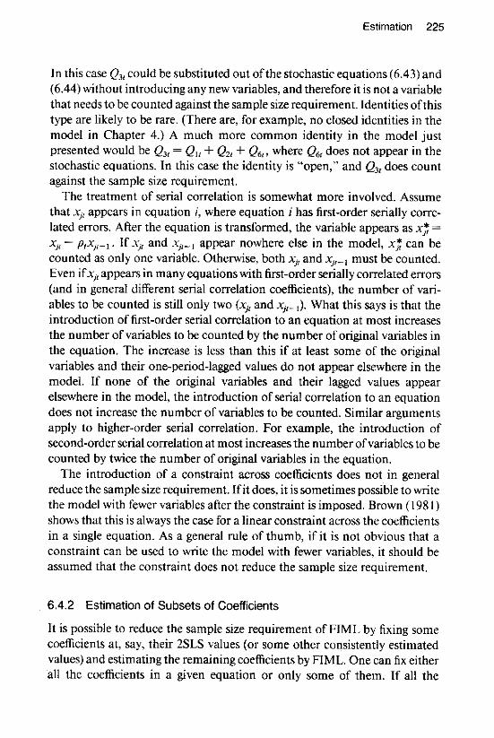
In this case Qx,, could be substituted out ofthe stochastic equations (6.43) and (6.44) without introducing any new variables, and therefore it is not a variable that needs to be counted against the sample size requirement. Identitiesofthis type are likely to be rare. (There are, for example, no closed identities in the model in Chapter 4.) A much more common identity in the model just presented would be f&, = Q1, + Q>, + Qs,. where QG, does not appear in the stochastic equations. In this case the identity is “open,” and f&,, does count against the sample size requirement.

The treatment of serial correlation is somewhat more involved. Assume that x, appears in equation i, where equation i has first-order serially correlated errors. After the equation is transformed, the variable appears as x; = xjt - pi.+, If xjt and xjz_l appear nowhere else in the model, x$ can be counted as only one variable. Otherwise, both xj, and x~,_~ must be counted. Even ifxjz appears in many equations with first-order serially correlated errors (and in general different serial correlation coefficients), the number of variables to be counted is still only two (xjz and x,_,). What this says is that the introduction of tint-order serial correlation to an equation at most increases the number of variables to be counted by the number of original variables in the equation. The increase is less than this if at least some of the original variables and their one-period-lagged values do not appear elsewhere in the model. If none of the original variables and their lagged values appear elsewhere in the model, the introduction of serial correlation to an equation does not increase the number of variables to be counted. Similar arguments apply to higher-order serial correlation. For example, the introduction of second-order serial correlation at most increases the number ofvariables to be counted by twice the number of original variables in the equation.

The introduction of a constraint across coefficients does not in general reduce the sample size requirement. If it does, it is sometimes possible to write the model with fewer variables after the constraint is imposed. Brown (198 1) shows that this is always the case for a linear constraint across the coefficients in a single equation. As a general rule of thumb, if it is not obvious that a constraint can be used to write the model with fewer variables, it should be assumed that the constraint does not reduce the sample size requirement.

6.4.2 Estimation of Subsets of Coefficients

It is possible to reduce the sample size requirement of FIML by fixing some coefficients at, say, their 2SLS values (or some other consistently estimated values) and estimating the remaining coefficients by FIML. One can fix either all the coefficients in a given equation or only some of them. If all the


coefficients are fixed, the equation is still taken to be part of the estimation problem in the sense that the covariance matrix Sin (6.33) is still n? X M, but none of the coefficients in the equation are estimated by FlML.

Consider the problem by estimating the free coefficients by F’IML, and write the relevant subset of the model as

(6.46) Q,A, = CT, >

where Q, is TX 41) A, is 9, X wzl, and C!~ is TX m, The matrix A, is the matrix of free coefficients, and m, is the number of equations in which at least one coefficient is free. CJ~, as will be seen, is the number of variables that count for purposes of calculating the sample size requirement. Its determination requires some explanation. Assume that x, and xk, appear in equation i and that their coefficients (ai, and LYJ are fixed. Assume that log ).‘;< is the LHS variable. This equation can be rewritten with logy,, - &xj, - h&t on the LHS and x,, and x, eliminated from the RHS. (cii, and 6, are the consistent estimates of Lyi, and (Y,~ .) If log Ye,, xj,, and xk, do not appear elsewhere in the model, this fixing of the coefficients has eliminated two variables. If log pir does appear elsewhere but xj, and x, do not, only one variable has been eliminated because the new LHS variable and log y;, count as separate variables. Ifx, and x,. appear elsewhere, no variables are eliminated. If all the coefficients in an equation are fixed, a variable in the equation is eliminated if it appears nowhere else in the model. 4, is the number of variables that remain after all possible eliminations.

Parke has shown that the sample size requirement for this reduced problem is T 2 q, + m2 - i, , where m2 = m - m, is the number of equations for which none ofthe coefficients are estimated and i, is the number of closed identities that pertain to the reduced set of equations (that is, the set of equations not counting the m2 equations for which no coefficients are estimated). Note that one observation is needed for each ofthe m2 equations that are not estimated.

Given this result, ifthe sample size requirement is not met for the complete model. the problem can be reduced by fixing various coefficients until it is met. An example of this procedure is presented in Section 6.52.

It should finally be noted that because of computational costs, one may want to restrict the size of the estimation problem even if the sample size requirement is met. The obvious way to do this is to fix some of the coefficients at their 2SLS estimates. This can be done for both the FIML and 3SLS estimators.

When only a subset of the coefficients is estimated by FIML or 3SLS, the easiest thing to do with regard to the estimation ofthe covariance matrix ofall

Estimation 227

the coefficient estimates is to assume that the coefficient estimates that are fixed with respect to the FIML or 3SLS estimation problem are uncorrelated with the FIML or 3SLS coefficient estimates. This allows the covariance matrix of all the coefficient estimates to be pieced together from the cover- iance matrix of the fixed estimates and the covariance matrix of the FIML or 3SLS estimates. Since correlation of coefficient estimates across equations is usually small relative to the correlation within an equation. the erron intro- duced by this procedure are likely to be fairly small in most applications. This is particularly true if the coefficient estimates that are fixed are of lesser importance than the others.

6.5 Computational Procedures and Results

6.5.1 OLS and 2SLS

For equations that are nonlinear in variables only, closed-form expressions exist for the OLS and 2SLS estimators. For 2SLS the expression is (6.9), and for OLS it is (6.9) with X;replacing fi. Ifthe nonlinearity in coefficients is due only to the presence of serially correlated error terms, the estimates can be obtained by solving (6.13) and (6.14) (or Eqs. 6.13’and 6.14’) or higher-order versions of these iteratively. For general nonlinearities in coefficients, (6.5) must be minimized using some general-purpose algorithm like the DFP algorithm discussed in Section 2.5.

Results.for the b’S Model

The 2SLS estimates of the US model are presented in Chapter 4. The first-stage regressors that were used for these estimates are given in Table 6-1. Two common sets are presented first in Table 6- 1, one for equations in which the RHS endogenous variables are primarily linear and one for equations in which the RHS endogenous variables are primarily in logarithms. The additional FSRs that were used for each equation are presented second. These FSRs are primarily variables that appear as explanatory variables in the equation being estimated but that are not part of the common set. The common sets include 34 variables, and the number of additional variables ranges from 0 to 9. The equations that are estimated by OLS have no RHS endogenous variables.

The time taken to estimate the 30 equations by 2SLS was about 3.0 minutes on the IBM 4341 and about 8.4 minutes on the VAX. The estimation ofthe covariance matrix ofall the coefficient estimates, vz in (6.20), took about 5.5

-


minutes on the IBM 4341 and about 7.8 minutes on the VAX. The derivatives in the Gi matrices that are needed for the estimation of the covariance matrix were computed numerically.

Eight of the 30 equations were estimated under the assumption of first- order serial correlation of the error terms. The iterative procedure described above was used. The starting value ofp was always zero, and the number of iterations required for convergence was 10, 7, 1 I> 4, 13, 6, 4, and 5 respectively. Convergence was defined to take place when successive estimates ofp were within .OOl of each other.

OLS estimation ofthe 30 equations took about .2 minutes on the IBM 434 1 and about .5 minutes on the VAX, which compares to about 3.0 and 8.4 minutes respectively for 2SLS estimation. The number of coefficients estimated in any one equation is small compared to the number estimated in the first-stage regressions, and this is the reason for the considerably larger expense of the 2SLS estimates. The maximum number of coefficients estimated in an equation is 12, whereas the minimum number estimated in a first-stage regression is 34. Nevertheless, the cost of 2SLS estimation is small relative to many other costs reported below.

6.5.2 FIML

Until recently the estimation of large nonlinear models by FIML was not computationally feasible, but this has now changed. The computational problem can be separated into two main parts: the first is to find a fast way of computing L in (6.33) for a given value of cy, and the second is to find an algorithm capable of maximizing L.

The main cost of computing L is computing the Jacobian term. Two savings can be made here. One is to exploit the sparseness ofthe Jacobian. The number of nonzero elements in J, is usually much less than nz. For the US model, for example, n is 128 (son* = 16,384), whereas the number of nonzero elements is only 441. Considerable computer time is saved by using sparse matrix routines to calculate the determinant ofJ,.

The second saving is based on an approximation. Consider approximating XL, loglJ,l by simply the average of the first and last terms in the summation

T multiplied by T: - (loglJ, I + loglJ,I). Let S,, denote the true summation, and

2 let S, denote the approximation. It turns out in the applications I have dealt with that S, - S, does not change very much as the coefficients change from their starting values (usually the 2SLS estimates) to the values that maximize

Estimation 231

the likelihood function. In other words, S, - S, is nearly a constant. This means that S, can be used instead of S,, in computing L, and thus considerable computer time is saved since the determinant ofthe Jacobian only needs to be computed twice rather than T times for each evaluation of L. For the US model T is 115. Using S, in place of S, means, of course. that the coefficient values that maximize the likelihood function are not the exact FIML estimates. If one is concerned about the accuracy ofthe approximation, one can switch from S, to S, after finding the maximum using S, If the approximation is good, one should see little further change in the coefficients: otherwise additional iterations using the algorithm will be needed to find the true maximum.

The choice of algorithm turns out to be crucial in maximizing L for large nonlinear models. My experience is that general-purpose algorithms like DFP do not work, and in fact the only algorithm that does seem to work is the Parke algorithm (1982a), which is a special-purpose algorithm designed for FIML and 3SLS estimation. This algorithm exploits two key features of models. The first is that the mean of a particular equation’s estimated residuals is approximately zero for the FIML and 3SLS estimates. For OLS this must be true, and empirically it turns out that it is approximately true for other estimators. The second feature is that the correlation of coefficient estimates within an equation is usually much greater than the correlation of coefficients across equations.

The problem with algorithms like DFP that require numerical first derivatives is that the computed gradients do not appear to be good guides regarding the directions to move in. Gradients are computed by perturbing one coefficient at a time. When a coefficient ischanged without the constant term in the equation also being changed to preserve the mean of the residuals, a large change in L results (and thus a large derivative). This result can obviously be quite misleading. The Parke algorithm avoids this problem by spending most of its time perturbing two coefficients at once, namely a given coefficient and the constant term in the equation in which the coefficient appears. The constant term is perturbed to keep the mean ofthe residualsunchanged. (The algorithm does not, of course. do this all the time, since the means of the residuals must also be estimated). To take advantage of the generally larger correlation within an equation than between equations, the Parke algorithm spends more time searching within equations than between them. General- purpose algorithms do not do this, since they have no knowledge of the structure of the problem.

It should also be noted regarding the computational problem that if only a


few coefficients are changed before a new value of L is computed, considerable savings can be made by taking advantage of this fact. If, for example, the coefficients are not in the Jacobian, the Jacobian term does not have to be recomputed. If only a few equations are affected by the change in coefficients, only a few rows and columns in the S matrix have to be recomputed. Since the Parke algorithm spends much of its time perturbing two coefficients at a time, it is particularly suited for these kinds of savings.

The estimated covariance matrix for the FIML coefficient estimates, p4 in (6.34) is difficult to compute. It is not part of the output of the Parke algorithm, and thus extra work is involved in computing it once the algorithm has found the optimum. My experience is that simply trying to compute the second derivatives of L numerically does not result in a positive-definite matrix. Although the true second-derivative matrices at the optimum are undoubtedly positive-definite, they seem to be nearly singular. If this is true, small errors in the numerical approximations to the second derivatives may be sufficient to make the matrix not positive-definite.

Fortunately, there is an approach to computing pd that does work, which is derived from Parke (1982a). Parke’s results suggest that the inadequate numerical approximations may be due to the fact that the means of the RHS variables in the estimated equations are not zero. If so, the problem can be solved by subtracting the means from the RHS variables before taking numerical derivatives. Let /I denote the coefficient vector that pertains to the model after the tneans have been subtracted, and let a denote the original coefficient vector. The relationship between (Y and p is

(6.47) CY=M./?,

where Mis a k X k square matrix that is composed ofthe identity matrix plus additional nonzero elements that represent the means adjustments. Unless there are constraints across equations, M is block-diagonal. Assume, for example, that the first equation of the model is

(6.48) Yl, = PI + Pz(Y21 - %) + Ps(Y,* - m3 + u,,, t=1,. ,I”,

where rn2 and ms are the sample means of yz, and Y,, respectively. This equation can be written

Estimation 233

In this case the part of (6.47) that corresponds to the first equation is

(6.50) (ii)-(s -” -r)(;;).

Parke found that the covariance matrix of B could easily be computed numerically. Let p&$) denote this matrix:

Given p&?), the covariance matrix of u is simply

(6.52) I$ = M. VJfl) M’.

p4 can thus be obtained by first computing the covariance matrix of the coefficients of the transformed model (that is, the model in which the RHS variables have zero means) and then using (6.52) to get the covariance matrix of the original coefficients.

Results for the US Model

The solution ofthe FIML estimation problem for the US model is reported in Table 6-2. Thereare 169 unconstrainedcoefficientsin the model: 107 ofthese were estimated by FIML, with the remaining tixed at their 2SLS estimates. The coefficients that were not estimated by FIML include the dummy variable coefficients in Eqs. I 1, 13, and 27 and all the coefficients in Eqs. 5,6. 7. 8. 15, lg. 19,20,21. 25, 28, and 29. These coefficients and equationswere judged to be less important than the others, although this is obviously a subjective choice. The sample size requirement for this subset ofcoefficients is 99. There are 115 observations.

The starting values were the 2SLS estimates. The value of L in (6.34) at these estimates is 5098.66. The change in L after 70 iterations in Table 6-2 is 18 I .76. On the first iteration the Parke algorithm increased L by 67.07, and on the second and third iterations it increased L by 8.68 and 7.64 respectively. The change after three iterations was thus 83.39. which is 45.9 percent ofthe total change. This illustrates ageneral feature ofthe Parke algorithm: it climbs very quickly for the first few iterations and then slows down considerably for the rest.

Between iterations 58 and 62 the number of Jacobians computed to approximate the sum was increased from 2 to 13. When I3 Jacobians were used, the sum was approximated by interpolating between the points. As can be seen in the table, the change in L was little affected by this. If the use of 2 Jacobians in fact provided a poor approximation, it is likely that the Parke algorithm would have increased L by much more than it did on the first few iterations after the switch. That it did not is some evidence in favor of the approximation.

Another way of looking at the 2 versus 13 question is to consider how sensitive the difference in L computed the two ways is to changes in the coefficients. The following results help answer this:

Estimation 235

V&e qf L 2 Jacobians

I. at start (ZSLS estimates) 5,098.66 L after 59 iterations L279.53 L after 62 iterations 5,279.82 L after 70 iterations 5,280.42

13 Jacobians

5,284.49 5,464.04 5.464.34 5,464.96

.!Aff^prmcr

- 185.83 -184.51 - 184.52 - 184.54

It is clear that the difference is little affected by the change in the coellicients from the 2SLS estimates to the estimates at the end of iteration 70. It thus seems that the use of 2 Jacobians is adequate. Note that this saves considerable time, since the cost ofone iteration ofthe Parke algorithm increases from about2.8 minutestoabout 5.4 minuteson theIBM4341 when 13 ratherthan 2 Jacobians are used.

As discussed earlier, when only one or two coefficients are being changed by the algorithm, many of the calculations involved in computingL do not have to be performed. In the present example, if these cost savings had not been used, the time taken for one iteration of the Parke algorithm would have increased by about a factor of 4.5, which is a considerable difference. As will be seen in the next section. this difference is even more pronounced in the 3SLS estimation problem.

It is a characteristic of the estimation problem that the likelihood function is fairly flat in the vicinity of the optimum. For example, the change in L on iteration 70 was only .06, and yet, as reported in note b in the table, 26 coefficients changed by 1 .O percent or more and 4 changed by 5.0 percent of more. The largest three changes were 8.1, 12.6, and 18.4 percent. The coefficients that change this much are obviously not significant, and they are not coefficients that are very important in the model. Nevertheless, these results do point out one of the reasons the FIML estimation problem is so hard to solve.

As noted in Table 6-2, the total time for the FIML estimation problem was about 3.5 hours on the IBM 4341. The time taken to compute the FIML covariance matrix after the coefficient estimates were obtained was about 53 minutes. The M transformation discussed earlier was used in the calculation of this matrix, and the second derivatives were obtained numerically.

6.5.3 3SLS

The 3SLS estimation problem is to minimize (6.24). The only cost saving to note for this problem is that the D matrix, which is M . TX m r, need not be calculated anew each time (6.24) is computed if only a few coefficients are changed.

Estimation 237

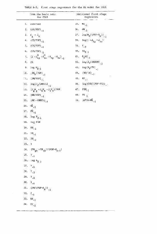
The first-stage regressors for this problem are presented in Table 6-3. There are 49 variables in this set. A number of the variables in Table 6-1 that were used for the 2SLS estimates were not used for the 3SLS estimates because of the desire to keep the number relatively small. The 2SLS estimates of the


residuals were used to compute 2 in (6.24), which remained unchanged throughout the solution of the problem.

The same subset ofcoefficients was estimated by 3SLS as was estimated by FIML. The solution of the 3SLS problem is reported in Table 6-4. This problem was easier to solve than the FIML problem. Again, the 2SLS estimates were used as starting values. The total change in the objective function, F, after 26 iterationswas46.55, ofwhich 39.81 was obtained by the Parke algorithm after 3 iterations. On iteration 26, eight coefficients changed by 1 .O percent or more, and the largest three changes were 6.6. 10.5, and 26.7 percent.

Each iteration requires about 4 minutes on the IBM 4341 and about 1 I minutes on the VAX. The total time for the 26 iterations on the IBM 4341 was about 1.7 hours. The D matrix for the US model is 3,450 X 3,450 (m = 30, T= 115), and considerable time was saved by not computing this matrix from scratch any more times than were absolutely necessary. If the entire matrix had been computed each time that (6.24) was computed, the time per iteration would have increased by about a factor of 17, and thus the total time would have increased from 1.7 hours to 28.9 hours.

The time taken to compute the 3SLS covariance matrix, ps in (6.25), was about 23 minutes on the IBM 4341 and about II minutes on the VAX. The derivative matrix d that is needed for this calculation was computed numerically. The reason the IBM 4341 time is large relative to the VAX time is that in the calculation of pa much reading and writing from the disk is done, and the IBM 4341 is relatively slow at this.

6.5.4 LAD and 2SLAD

The LAD and 2SLAD computational problem is to minimize

(6.53) 2 hl

with respect to oi, where uil = ud = y, - h, for LAD and u, = qyil + (I - y)gft - 6, for 2SLAD. This computational problem is not particularly easy, especially when uil is a nonlinear function ofol,. I have had no success in trying to minimize(653)using theDFPalgorithm and Powell’s no-derivative algorithm (1964). (When the DFP algorithm was tried, the derivatives were computed numerically. The problem that they do not exist everywhere was ignored.) Both algorithms failed to get close to the optimum in most of the cases that I tried.

Estimation 239

Because the standard algorithms do not work, other approaches must be tried. I have used two, one that worked well and one that did not. The one that worked well uses the fact that

where vvi, = /I+~/. For a given set of values of ivi, (t = 1, , T), minimizing (6.54) is simply a weighted least squares problem. If vi, is a linear function of cyj, closed-form expressions exist for &; otherwise a nonlinear optimization algorithm can be used. This suggests the following iterative procedure. (I) Pick an initial set of values of wit These can be the absolute values of the OLS or 2SLS estimated residuals. (2) Given these values, minimize (6.54). (3) Given the estimate of oli from step 2, compute new values of vi, and thus new values of +v>(. (4) With the new weights, go back to step 2 and minimize (6.54) again. Keep repeating steps 2 and 3 until successive estimates ofcvi are within some prescribed tolerance level. If on any step some value of uSi, is smaller than some small preassigned number (say E). the value of wi, should be set equal to E.

The accuracy of the estimates using this approach is a function of E: the smaller is E, the greater is the accuracy. If vi, is a linear function of ol;, the estimates will never be exact because the true estimates correspond to ki values of u~,~ being exactly zero, where ki is the number of elements of ai.

In the case in which the equation to be estimated is linear in coefficients, the closed-form expression for & for a given set of values of ivir is

(6.55) &, = &,,@-r,$yj+

2: is the same as ,?i in (6.9) except that each element in row t of.$ is divided by 6. The vector dt equals ~JJ~ + (I - q)jJj except that row 1 is divided by J;;,. ($i equals D(JI .)

Ifthe equation is linear in coefficients but has serially correlated errors: vi, is not a linear function of the coefficients inclusive of the serial correlation coefficients. and therefore a closed-form expression does not exist. It is possible in his case, however, to solve for the estimates by iteratively solving equations like (6.13) and (6.14). This avoids having to use a general-purpose algorithm like DFP. Assuming that Xi_, and yi_, are included in Z,, the two equations for the first-order serial correlation case are

(6.57) j& = a


\,

“\;-“: -B

P

L Figure 6-I Approximation ofA@,, .L3) to Iq,l

,?T* is the matrix $ - Xi_l& with each element in row t divided by Gt; &* is the vector qyi + (1 - q).& - y,_,j, with row I divided by &,; ii?-, is the vector yi_, - Xii_& with row I divided by Jk;;;; and t$ is the vector qy, + (1 - q)ji - Xii$ with row I divided by &,. For a given set of weights, (6.56) and (6.57) can be solved iteratively.

The second approach is derived from Tishler and Zang (1980). The prob lem of minimizing (6.53) is changed to a problem of minimizing

-4 if q, 5 --I( (6.59) 4%,8) =

I (L'Z +P*)/u if-/?<v,,</J. 0, if uif 2fl

The value ofpis some small preassigned number. Since lim A(+,# =IuJ, the

smaller isp, the closer is (6.53) to (6.59). The approxim%& ofA(v,, /I’) tolq,;,l is presented in Figure 6-I. Since A(+, p) is once continuously differentiable, an optimization algorithm like DFP can be used to minimize (6.59) for a given value of p, The smaller is 8, the more difficult the minimization problem is likely to be_ and thus there is a trade-off between accuracy and ease of solution.

Estimation 241

Four sets of estimates of the US model were obtained: LAD, 2SLAD using 4 = 0.0, 2SLAD using q = 0.5, and 2SLAD using 4 = 1 .O. The method of Tishler and Zang did not work well, in the sense that the results were quite sensitive to the value ofg chosen, and therefore it was dropped from further consideration fairly early in the calculations. For small values offi the DFF’ algorithm, which was the algorithm used, failed to converge, and for large values of fi the algorithm converged to answers that implied values of the true objective function, (6.53), that were larger than those obtained by the first method. It was difficult to find in-between values ofa that worked well.

The first method, on the other hand, worked extremely well. For ZSLAD using 4 = 0.5, for example, the number ofiterations required for convergence for the 30 equations ranged from 4 to 145, with an average of 35.6. Conver- gence was taken to be achieved when successive estimates ofeach coefficient were within .002 percent of each other. The value used for E was .OOOOOOl. The total time for estimating the model by LAD was about 2.2 minutes on the IBM 4341 and about 5.7 minutes on the VAX. The total time for each ofthe three 2SLAD estimation problems was about 6.5 minutes on the IBM 4341 and about 16.5 minutes on the VAX. Of the 120 equations estimated, none had a residual that was smaller than E in absolute value at the time that convergence was achieved. These results are very encouraging, and they indicate that computational costs are not likely to be a serious problem in the future with respect to LAD and 2SLAD estimation.

6.6 Comparison of the OLS, 2SLS, 3SLS, FIML, LAD, and 2SLAD Results for the US Model

If the model is correctly specified and all the assumptions about the error terms are correct, all but the OLS and LAD estimates of the US model are consistent. They should thus differ from each other only because of a finite sample size. In practice the model is likely to be misspecihed. and not all the assumptions about the error terms are likely to be correct. Given this, it is not obvious how the estimates should compare. In this section the quantitative differences among the estimates are examined. The consequences of these differences for the predictive accuracy of the model are discussed in Section 8.5.5, and the consequences for the properties of the model are discussed in Section 9.4.5.

Table 6-5 presents acomparison ofthe estimates for six equations: the three consumption equations, 1, 2. and 3; the price equation. 10; the production

- _ -

Estimation 243

equation, 11; and the interest rate reaction function, 30. The 2SLS estimates are used as the basis ofcomparison. Each number in a “b” column in the table is the difference between the particular estimate and the 2SLS estimate divided by the standard error of the 2SLS estimate. These numbers thus indicate how many standard errors the estimates are from the 2SLS estimates. where the standard errors that are used are 2SLS standard errors. Table 6-6 provides summary measures for all the coefficient estimates.

The main conclusion to be drawn from these results is that all the estimates are fairly close to each other except for the F’IML estimates. Consider Table 6-6: only 3 of the 107 3SLS coefficient estimates are more than 1.5 standard errors away from the 2SLS estimates, whereas 38 ofthe RML estimates are. Only 1 ofthe 169 OLS estimatesismore than 1.5 standard errorsaway. Ofthe 2SLAD estimates, 7 are more than 1.5 standard errors away for 4 = 0.0, 12 are forq=0.5, and 19 are forq = 1.0. For LAD the number is 15. Very fewofthe estimates changed signs, as can be seen in the bottom half of Table 6-6. Even for FIML_ only 6 estimates changed sign.

With respect to the individual estimates in Table 6-5, one important difference between the FIML estimates and the others occurs in Eq. 11, the equation determining production, Y. Coefficient 3 in Eq. 1 I is the coefficient for the sales variable, X. For all the estimates except FIML, this coefficient is around 1 .O, whereas for FIML it is around I .4. Also, coefficient 2 in Eq. 1 I _ which is the coefficient of the lagged dependent variable, is around .I5 for the other estimates and close to zero for FIML. The FIML estimates of the lagged dependent variable coefficients in two of the three consumption equations (Eqs. 2 and 3) are likewise quite different from the others. In both equations the lagged dependent variable coefficient is number 2. The FIML and 2SLS estimates in the two equations are. respectively, ,666 I9 versus .4 1164 and .45821 versus .07423.

It should be stressed that the only reason for the present comparison is to get a general idea of how close the estimates are. Of more importance are the comparisons in Sections 8.5.5 and 9.4.5, which examine the estimates within the context of the overall model. What can be said so far is that the RML estimates differ most from the others when the examination is coefficient by coefficient.

Comparison ofStandard Errors

Table 6-7 presents a comparison of the 2SLS. 3SLS, and RML estimated standard errors. As expected, the 2SLS standard errors are generally larger


than the 3SLS standard errors_ where the average of the ratios of the two is I .27. This is not always the case, however, as can be seen for coefficients l-6 and 8 in Eq. 4, where the 2SLS standard errors are smaller. This difference is due to the different first-stage regressors that are used by 2SLS and 3SLS. As discussed earlier, 2SLS uses different sets of FSRs for different equations, whereas 3SLS uses a common set that is smaller than the union of the 2SLS sets. This can cause the 2SLS standard errors to be smaller. In the present case, Eq. 4 has no RHS endogenous variables, and thus the 2SLS estimates are the OLS estimates. The FSRs in this case include all the explanatory variables in the equation. Not all of these explanatory variables were included in the common set of FSRs for the 3SLS estimates, and therefore some of the variables in the equation were treated as endogenous. This was enough to lead to larger 3SLS standard errors for some of the coefficients.

The more interesting result in Table 6-7 is that the 3SLS standard errors are generally smaller than the FIML standard errors. The average of the ratios of the two is .74. This result has also been obtained, but not discussed, by Hausman (I 974). For 10 of the 12 estimated coefficients of Klein’s model I that are reported in Hausman’s table 1, p. 649, the FIML standard error is larger than the corresponding 3SLS standard error.

My conjecture as to why the 3SLS standard errors are generally smaller is the following. Given the large number of FSRs that are used by 3SLS, the predicted values of the endogenous variables from the first-stage regressions are fairly close to the actual values. For FIML, on the other hand, we know from Hausman’s interpretation (1975) of the FIML estimator as an instru-


mental variables estimator that FIML takes into account the nonlinear restrictions on the reduced form coefficients in forming the instruments. This means that in small samples the instruments that FIML forms are likely to be based on worse first-stage fits of the endogenous variables than are the instruments that 3SLS forms. In a loose sense, this situation is analogous to the fact that in the 2SLS case the more variables that are used in the first-stage regressions. the better is the tit in the second-stage regression.

Possible Use cfrhr Huusman Test

An interesting question is whether Hausman’s m-statistic (1978) provides a useful way of examining the differences among the estimates. The m-statistic is as follows. Consider two estimators, j0 and /?, , where under some null hypothesis both estimators are consistent but only ,$ is asymptotically effi- tient. -while under the alternative hypothesis only pi is consistent. Let 4 = /J’, - /la, and let V. and vt denote consistent estimates of the asymptotic covariance matrices ( vr, and Vi) of ,$, and ,&, respectively. Hausman’s m-statistic is @(v, - VJ’@, and he has shown that it is asymptotically distributed as x2 with k degrees of freedom, where k is the dimension of 8. Note that under the null hypothesis V, - V. is positive-definite.

Consider now comparing the FIML and 3SLS estimates. Under the null hypothesis of correct specification and normally distributed errors, both estimates are consistent, but only the FIML estimates are asymptotically efficient. On the other hand, 3SLS estimates are consistent for a broad class of error distributions, whereas for many distributions FIML estimates are inconsistent. If the alternative hypothesis is taken to be that the error distribution is one that leads to consistent 3SLS estimates but inconsistent FIML estimates, then in principle Hausman’s m-statistic can be used to test the null hypothesis of normality against the alternative. Let W) and d@) denote the 3SLS and FIML estimates of (Y respectively, and let rj = &(a) - &@J, The m-statistic in this case is $(ps - pJi& where the estimated covariance matrices vJ and p* are defined in (6.25) and (6.34) respectively.

In practice the test cannot be performed if pr - pg is not positive-definite. For the US model it is clear from Table 6-7 that pr - pa is not positive-deft- nite, since most of the diagonal elements of pr are smaller than the corresponding elements of vd. Ifanything, & - pa is closer to being negative-deft- nite, although this is not true either since some of the diagonal elements of pd are smaller than the corresponding elements of pa The matrix Pa - vd is also not positive-definite for Klein’s model I. since, as noted earlier, Hausman’s

Estimation 247

results (I 974) show that 10 of the 12 estimated coeffcients have larger FlML standard errors than 3SLS standard errors. It thus seems unlikely that 1’, - pd will be positive-definite in practice for most models, and therefore the m-statistic is not likely to be useful for testing the normality hypothesis. (If the model is linear, the test obviously has no power, since RML, like 3SLS, is consistent for a broad class of error distributions.)

The m-statistic can also be used in principle to compare the FIML and 2SLS estimates. Under the null hypothesis of normally distributed errors and correct specification, both estimates are consistent, but only the FIML estimates are asymptotically efficient. Under the alternative hypothesis of normality and misspecification of some subset of the equations, all the FIML estimates are inconsistent, but only the ZSLS estimates of the misspecitied subset are inconsistent. The m-statistic can thus be applied to one or more equations at a time to test the hypothesis that the rest ofthe model is correctly specified. If for some subset the m-statistic exceeds the critical value, the test would indicate that there is misspecification somewhere in the rest of the model.

In practice this test cannot be applied if pz - fd is not positive-definite, and for the US model, as is clear from Table 6-7, vz - PA is not positive-definite, Many of the diagonal elements of vz are smaller than the corresponding elements of pa. It thus also seems unlikely that this test of misspecification will be useful in practice.

Finally, the specification hypothesis can be tested in certain circumstances using the m-statistic on the 2SLS and 3SLS estimates. Ifboth estimators are members of a class of estimators for which 3SLS is asymptotically efficient. the test can be applied. The problem is that when the two estimators are based on different sets of FSRs, as is usually the case with large models, they are not members of the same class. One cannot argue. for example, that the 3SLS estimates given above for the US model are asymptotically efficient relative to the 2SLS estimates, and thus the Hausman test cannot be applied in this case.

In summary, the m-statistic does not seem useful for testing either the normality hypothesis or the correct specification hypothesis. Regarding the latter, my feeling is that it is better simply to assume that the model is misspecified (so that no test is needed) and to try to estimate the degree of misspecification. This is the procedure followed for the comparison method in Chapter 8.

Documents

6 Estimation - fairmodel.econ.yale.edu