Embed Size (px)
Citation preview
5.3 The Definite Integral 343
The Definite Integral
In Section 5.2 we investigated the limit of a finite sum for a function defined over a closedinterval [a, b] using n subintervals of equal width (or length), In this sectionwe consider the limit of more general Riemann sums as the norm of the partitions of [a, b]approaches zero. For general Riemann sums the subintervals of the partitions need nothave equal widths. The limiting process then leads to the definition of the definite integralof a function over a closed interval [a, b].
Limits of Riemann Sums
The definition of the definite integral is based on the idea that for certain functions, as thenorm of the partitions of [a, b] approaches zero, the values of the corresponding Riemann
sb - ad>n .
5.3
sums approach a lim
iting value I. What w
e mean by this converging idea is that a R
iemann
sum w
ill be close to the number I
provided that the norm of its partition is sufficiently
small (so that all of its subintervals have thin enough w
idths). We introduce the sym
bol as a sm
all positive number that specifies how
close to Ithe R
iemann sum
must be, and the
symbol
as a second small positive num
ber that specifies how sm
all the norm of a parti-
tion must be in order for that to happen. H
ere is a precise formulation.
d
P
344Chapter 5: Integration
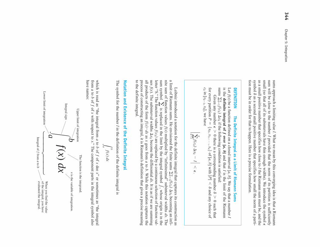
DEFINITION
The Definite Integral as a Limit of Riem
ann Sums
Let ƒ(x) be a function defined on a closed interval [a,b]. W
e say that a number I
is the definite integral of ƒover [a,
b]and that I
is the limit of the R
iemann
sums
if the following condition is satisfied:
Given any num
ber there is a corresponding num
ber such that
for every partition of [a,b] w
ith and any choice of
in w
e have
`a n
k=1 ƒsc
k d ¢x
k-
I `6
P.
[xk-
1 , xk ],
ck
7P 76d
P=5
x0 , x
1 ,Á, x
n 6d
70
P7
0g
nk=1 ƒsc
k d ¢x
k
Leibniz introduced a notation for the definite integral that captures its construction as
a limit of R
iemann sum
s. He envisioned the finite sum
s becom
ing an infi-nite sum
of function values ƒ(x) multiplied by “infinitesim
al” subinterval widths dx. T
hesum
symbol
is replaced in the limit by the integral sym
bol w
hose origin is in theletter “S
.” The function values
are replaced by a continuous selection of function val-ues ƒ(x). T
he subinterval widths
become the differential dx. It is as if w
e are summ
ingall products of the form
as x
goes from a
to b. While this notation captures the
process of constructing an integral, it is Riem
ann’s definition that gives a precise meaning
to the definite integral.
Notation and Existence of the Definite Integral
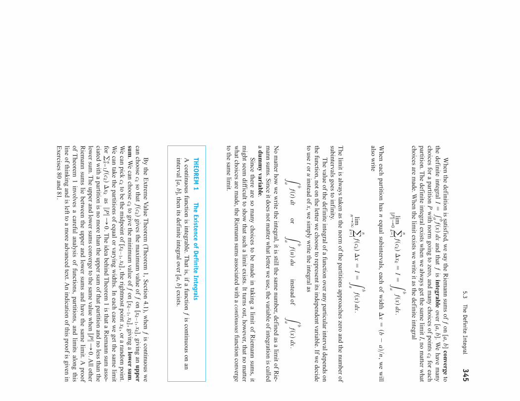
The sym
bol for the number I
in the definition of the definite integral is
which is read as “the integral from
ato b
of ƒof x
dee x” or sometim
es as “the integralfrom
ato b
of ƒof x
with respect to x.” T
he component parts in the integral sym
bol alsohave nam
es:
⌠⎮⎮⌡
⎧⎪⎪⎨⎪⎪⎩
The function is the integrand.
x is the variable of integration.
When you find the value
of the integral, you haveevaluated the integral.
Upper lim
it of integration
Integral sign
Low
er limit of integration
Integral of f from a to b
a bf(x) dx
Lb
aƒsxd dx
ƒsxd #dx ¢x
k
ƒsck d
1,
ag
nk=1 ƒsc
k d ¢x
k
When the definition is satisfied, w
e say the Riem
ann sums of ƒ
on [a,b] convergeto
the definite integral and that ƒ
is integrableover [a,b]. W
e have many
choices for a partition Pw
ith norm going to zero, and m
any choices of points for each
partition. The definite integral exists w
hen we alw
ays get the same lim
it I, no matter w
hatchoices are m
ade. When the lim
it exists we w
rite it as the definite integral
When each partition has n
equal subintervals, each of width
we w
illalso w
rite
The lim
it is always taken as the norm
of the partitions approaches zero and the number of
subintervals goes to infinity.T
he value of the definite integral of a function over any particular interval depends onthe function, not on the letter w
e choose to represent its independent variable. If we decide
to use tor uinstead of x, w
e simply w
rite the integral as
No m
atter how w
e write the integral, it is still the sam
e number, defined as a lim
it of Rie-
mann sum
s. Since it does not m
atter what letter w
e use, the variable of integration is calleda dum
my variable.
Since there are so m
any choices to be made in taking a lim
it of Riem
ann sums, it
might seem
difficult to show that such a lim
it exists. It turns out, however, that no m
atterw
hat choices are made, the R
iemann sum
s associated with a continuous
function convergeto the sam
e limit.
Lb
aƒstd dt
or L
b
aƒsud du
instead of L
b
aƒsxd dx.
limn:
q a n
k=1 ƒsc
k d ¢x
=I=L
b
aƒsxd dx. ¢
x=sb
-ad>n
,
limƒƒ P
ƒƒ :0 a n
k=1 ƒsc
k d ¢x
k=
I=L
b
aƒsxd dx.
ck
I=1
baƒsxd dx
5.3The Definite Integral
345
THEOREM
1The Existence of Definite Integrals
A continuous function is integrable. T
hat is, if a function ƒis continuous on an
interval [a,b], then its definite integral over [a,b] exists.
By the E
xtreme V
alue Theorem
(Theorem
1, Section 4.1), w
hen ƒis continuous w
ecan choose
so that gives the m
aximum
value of ƒon
giving an uppersum
. We can choose
to give the minim
um value of ƒ
on giving a low
er sum.
We can pick
to be the midpoint of
the rightmost point
or a random point.
We can take the partitions of equal or varying w
idths. In each case we get the sam
e limit
for as
The idea behind T
heorem 1 is that a R
iemann sum
asso-ciated w
ith a partition is no more than the upper sum
of that partition and no less than thelow
er sum. T
he upper and lower sum
s converge to the same value w
hen A
ll otherR
iemann sum
s lie between the upper and low
er sums and have the sam
e limit. A
proofof T
heorem 1 involves a careful analysis of functions, partitions, and lim
its along thisline of thinking and
is left to a more advanced text. A
n indication of this proof is given inE
xercises 80 and 81.
7P 7:0
.
7P 7:0
.g
nk=1 ƒsc
k d ¢x
k
xk ,
[xk-
1 , xk ],
ck
[xk-
1 , xk ],
ck
[xk-
1 , xk ],
ƒsck d
ck
Theorem
1 says nothing about how to calculate
definite integrals. A m
ethod of calcu-lation w
ill be developed in Section 5.4, through a connection to the process of taking anti-
derivatives.
Integrable and Nonintegrable Functions
Theorem
1 tells us that functions continuous over the interval [a,b] are integrable there.F
unctions that are not continuous may or m
ay not be integrable. Discontinuous functions
that are integrable include those that are increasing on [a,b] (Exercise 77), and the
piecewise-continuous functions
defined in the Additional E
xercises at the end of this chap-ter. (T
he latter are continuous except at a finite number of points in [a,b].) For integrabil-
ity to fail, a function needs to be sufficiently discontinuous so that the region between its
graph and the x-axis cannot be approximated w
ell by increasingly thin rectangles. Here is
an example of a function that is not integrable.
EXAMPLE 1
A Nonintegrable Function on [0, 1]
The function
has no Riem
ann integral over [0, 1]. Underlying this is the fact that betw
een any two num
-bers there is both a rational num
ber and an irrational number. T
hus the function jumps
upand dow
n too erratically over [0, 1] to allow the region beneath its graph and above the
x-axis to be approximated by rectangles, no m
atter how thin they are. W
e show, in fact, that
upper sum approxim
ations and lower sum
approximations converge to different lim
itingvalues.
If we pick a partition P
of [0, 1] and choose to be the m
aximum
value for ƒon
then the corresponding Riem
ann sum is
since each subinterval contains a rational num
ber where
Note that the
lengths of the intervals in the partition sum to 1,
So each such R
iemann
sum equals 1, and a lim
it of Riem
ann sums using these choices equals 1.
On the other hand, if w
e pick to be the m
inimum
value for ƒon
then theR
iemann sum
is
since each subinterval contains an irrational num
ber w
here T
helim
it of Riem
ann sums using these choices equals zero. S
ince the limit depends on the
choices of the function ƒ
is not integrable.
Properties of Definite Integrals
In defining as a lim
it of sums
we m
oved from left to right
across the interval [a,b]. What w
ould happen if we instead m
ove right to left, starting with
and ending at E
ach in the R
iemann sum
would change its sign, w
ithnow
negative instead of positive. With the sam
e choices of in each subinter-
val, the sign of any Riem
ann sum w
ould change, as would the sign of the lim
it, the integralc
kx
k-
xk-
1
¢x
kx
n=
a.
x0=
b
gnk=
1 ƒsck d ¢
xk ,
1baƒsxd dx
ck ,
ƒsck d
=0
.c
k[x
k-1 , x
k ]
L=a n
k=1 ƒsc
k d ¢x
k=a n
k=1 s0d ¢
xk=
0,
[xk-
1 , xk ],
ck
gnk=
1 ¢x
k=
1. ƒsc
k d=
1.
[xk-
1 , xk ]
U=a n
k=1 ƒsc
k d ¢x
k=a n
k=1 s1d ¢
xk=
1,
[xk-
1 , xk ]
ck
ƒsxd=e
1,if x is rational
0,if x is irrational
346Chapter 5: Integration

Since w
e have not previously given a meaning to integrating backw
ard, we are
led to define
Another extension of the integral is to an interval of zero w
idth, when
Since
is zero when the interval w
idth , w
e define
Theorem
2 states seven properties of integrals, given as rules that they satisfy, includ-ing the tw
o above. These rules becom
e very useful in the process of computing integrals.
We w
ill refer to them repeatedly to sim
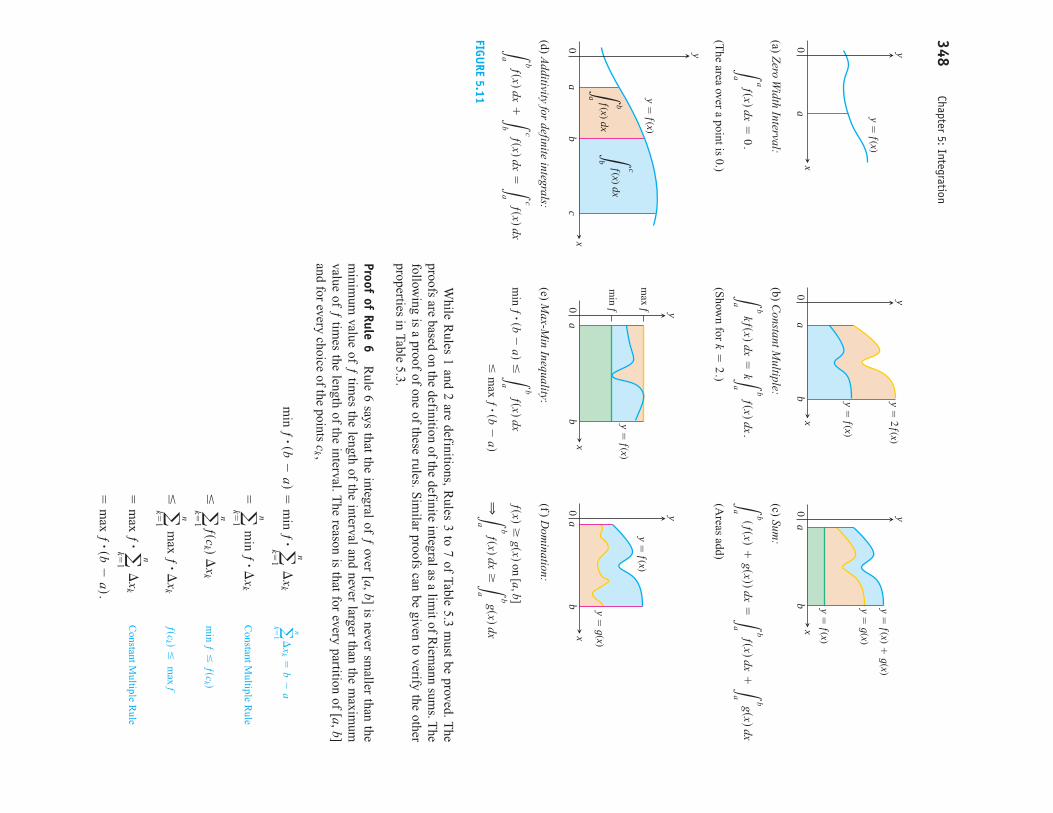
plify our calculations.R
ules 2 through 7 have geometric interpretations, show
n in Figure5.11. T
he graphs inthese figures are of positive functions, but the rules apply to general integrable functions.
La
aƒsxd dx
=0
.
¢x
k=
0ƒsc
k d ¢x
k
a=
b.
La
bƒsxd dx
=-L
b
aƒsxd dx.
1abƒsxd dx.
5.3The Definite Integral
347
THEOREM
2W
henƒ
andg
areintegrable,the
definiteintegralsatisfies
Rules
1to
7in
Table5.3.
TABLE 5.3Rules satisfied by definite integrals
1.O
rder of Integration:A
Definition
2.Z
ero Width Interval:
Also a D
efinition
3.C
onstant Multiple:
Any N
umber k
4.Sum
and Difference:
5.A
dditivity:
6.M
ax-Min Inequality:
If ƒhas m
aximum
value max
ƒand m
inimum
value m
in ƒon [a,b], then
7.D
omination:
(Special C
ase)ƒsxd
Ú0 on [a, b] Q
Lb
aƒsxd dx
Ú0
ƒsxdÚ
gsxd on [a, b] Q L
b
aƒsxd dx
ÚLb
agsxd dx
min ƒ #sb
-ad
…Lb
aƒsxd dx
… m
ax ƒ #sb-
ad.
Lb
aƒsxd dx
+Lc
bƒsxd dx
=Lc
aƒsxd dx
Lb
asƒsxd
;gsxdd dx
=Lb
aƒsxd dx
;Lb
agsxd dx
k=
-1
Lb
a -
ƒsxd dx=
-Lb
aƒsxd dx
Lb
akƒsxd dx
=kL
b
aƒsxd dx
La
aƒsxd dx
=0
La
bƒsxd dx
=-L
b
aƒsxd dx
While R
ules 1 and 2 are definitions, Rules 3 to 7 of Table 5.3
must be proved. T
heproofs are based on the definition of the definite integral as a lim
it of Riem
ann sums. T
hefollow
ing is a proof of one of these rules. Sim
ilar proofs can be given to verify the otherproperties in Table 5.3.
Proof of Rule 6R
ule 6 says that the integral of ƒover [a,b] is never sm
aller than them
inimum
value of ƒtim
es the length of the interval and never larger than the maxim
umvalue of ƒ
times the length of the interval. T
he reason is that for every partition of [a,b]and for every choice of the points
Constant M
ultiple Rule
Constant M
ultiple Rule
=m
ax ƒ #sb-
ad.
=m
ax ƒ #a n
k=1 ¢
xk
ƒsck d
… m
ax f …a n
k=1 m
ax ƒ #¢x
k
min ƒ
…ƒsc
k d …a n
k=1 ƒsc
k d ¢x
k
=a n
k=1 m
in ƒ #¢x
k
a n
k=1 ¢
xk=
b-
a m
in ƒ #sb-
ad=
min ƒ #a n
k=1 ¢
xk
ck ,
348Chapter 5: Integration
x
y0a y �
f(x)
x
y0a
b y � f(x)
y � 2f(x)
x
y0a
b y � f(x)
y � f(x) �
g(x)
y � g(x)
x
y0a
cb
y � f(x)
b
a f(x) dxf(x) dx
Lc
bL
x
y0a
b y � f(x)
max f
min f
x
y0a
b
y � f(x)
y � g(x)
FIGURE 5.11
(a) Zero W
idth Interval:
(The area over a point is 0.)
La
aƒsxd dx
=0
.
(b) Constant M
ultiple:
(Show
n for )
k=
2.
Lb
a kƒsxd dx
=kL
b
a ƒsxd dx
.
(c) Sum:
(Areas add)
Lb
asƒsxd
+gsxdd dx
=Lb
aƒsxd dx
+Lb
agsxd dx
(d) Additivity for definite integrals:
Lb
aƒsxd dx
+Lc
bƒsxd dx
=Lc
aƒsxd dx
(e) Max-M
in Inequality:
…m
ax ƒ #sb
-ad
min
ƒ #sb-
ad…L
b
a ƒsxd dx
(f) Dom
ination:
QLb
a ƒsxd dx
ÚLb
a gsxd dx
ƒsxdÚ
gsxd on [a, b]
In short, all Riem
ann sums for ƒ
on [a,b] satisfy the inequality
Hence their lim
it, the integral, does too.
EXAMPLE 2
Using the Rules for Definite Integrals
Suppose that
Then
1.R
ule 1
2.R
ules 3 and 4
3.R
ule 5
EXAMPLE 3
Finding Bounds for an Integral
Show
that the value of is less than
.
SolutionT
heM
ax-Min
Inequalityfordefinite
integrals(R
ule6)says
that
is a lower bound
for the value of and that
is an upper bound.
The m
aximum
value of on [0, 1] is
so
Since
is bounded from above by
(which is 1.414
), the integralis less than
.
Area Under the Graph of a N
onnegative Function
We now
make precise the notion of the area of a region w
ith curved boundary, capturingthe idea of approxim
ating a region by increasingly many rectangles. T
he area under thegraph of a nonnegative continuous function is defined to be a definite integral.
3>2Á
22
110 2
1+
cos x dx
L1
0 21
+cos x dx
…22 #s1
-0d
=22
.
21
+1
=22
,2
1+
cos x
max ƒ #sb
-ad
1baƒsxd dx
min ƒ #sb
-ad
3>21
10 21
+cos x dx
L4
-1 ƒsxd dx
=L1
-1 ƒsxd dx
+L4
1ƒsxd dx
=5
+s-
2d=
3
=2s5d
+3s7d
=31
L1
-1 [2ƒsxd
+3hsxd] dx
=2L
1
-1 ƒsxd dx
+3L
1
-1 hsxd dx
L1
4ƒsxd dx
=-L
4
1ƒsxd dx
=-s-
2d=
2
L1
-1 ƒsxd dx
=5,
L4
1ƒsxd dx
=-
2, L
1
-1 hsxd dx
=7
.
min ƒ #sb
-ad
…a n
k=1 ƒsc
k d ¢x
k…
max ƒ #sb
-ad.
5.3The Definite Integral
349
DEFINITION
Area Under a Curve as a Definite Integral
If is nonnegative and integrable over a closed interval [a,b], then the
area under the curve over [a,b] is the integral of ƒ
from a
to b,
A=L
b
aƒsxd dx.
y=
ƒsxdy
=ƒsxd
For the first time w
e have a rigorous definition for the area of a region whose bound-
ary is the graph of any continuous function. We now
apply this to a simple exam
ple, thearea under a straight line, w
here we can verify that our new
definition agrees with our pre-
vious notion of area.
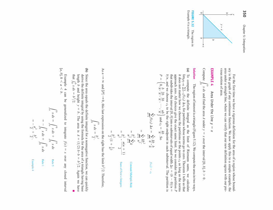
EXAMPLE 4
Area Under the Line
Com
pute and find the area A
under over the interval [0,b],
SolutionT
heregion
ofinterestisa
triangle(Figure
5.12).We
compute
thearea
intw
o ways.
(a)To
compute
the definite
integral as
the lim
it of
Riem
ann sum
s, w
e calculate
for partitions whose norm
s go to zero. Theorem
1 tells us thatit does not m
atter how w
e choose the partitions or the points as long as the norm
sapproach zero. A
ll choices give the exact same lim
it. So w
e consider the partition Pthatsubdivides
theinterval[0,b]into
nsubintervals
ofequalwidth
and we choose
to be the right endpoint in each subinterval. The partition is
and S
o
Constant M
ultiple Rule
Sum
of First nIntegers
As
and this last expression on the right has the lim
it T
herefore,
(b)S
ince the area equals the definite integral for a nonnegative function, we can quickly
derive the definite integral by using the formula for the area of a triangle having base
length band height
The area is
Again w
e have
that
Exam
ple 4
can be
generalized to
integrate over
any closed
interval
Rule 5
Rule 1
Exam
ple 4 =
-a
22+
b22.
=-L
a
0x dx
+Lb
0x dx
Lb
ax dx
=L0
ax dx
+Lb
0x dx
[a, b], 06
a6
b.
ƒsxd=
x
1b0 x dx
=b
2>2.A
=s1>2d b #b
=b
2>2.
y=
b.
Lb
0x dx
=b
22.
b2>2.
7P 7:0
,n:
q
=b
22 s1
+1n d
=b
2
n2 # nsn
+1d
2
=b
2
n2 a n
k=1 k
=a n
k=1 kb
2
n2
ƒsck d
=c
k a n
k=1 ƒsc
k d ¢x
=a n
k=1 kbn
# bn
ck=
kbn.
P=e
0, bn, 2bn
, 3bn, Á
, nbn fc
kb>n
,¢
x=sb
-0d>n =
ck
limƒƒ Pƒƒ :
0 gnk=
1 ƒsck d ¢
xk
b7
0.
y=
xL
b
0x dx
y=
x
350Chapter 5: Integration
x
y0 b
b b
y � x
FIGURE 5.12
The region in
Exam
ple 4 is a triangle.
In conclusion,we have the follow
ing rule for integrating f(x)=
x:
5.3The Definite Integral
351
(1)L
b
ax dx
=b
22-
a22,
a6
b
This com
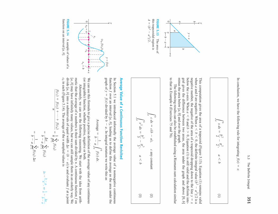
putation gives the area of a trapezoid (Figure5.13). E
quation (1) remains valid
when a
and bare negative. W
hen the definite integral value
is anegative num
ber, the negative of the area of a trapezoid dropping down to the line
below the x-axis. W
hen and
Equation (1) is still valid and the definite inte-
gral gives the difference between tw
o areas, the area under the graph and above [0,b]m
inus the area below [a, 0] and over the graph.
The follow
ing results can also be established using a Riem
ann sum calculation sim
ilarto that in E
xample 4 (E
xercises 75 and 76).
b7
0,
a6
0y
=x
sb2-
a2d>2
a6
b6
0,
(2)
(3)L
b
ax
2 dx=
b33
-a
33,
a6
b
Lb
ac dx
=csb
-ad,
c any constant
x
y0 a
a
b
b
a
b
b � a
y � x
FIGURE 5.13
The area of
this trapezoidal region isA
=sb
2-
a2d>2
.
Average Value of a Continuous Function Revisited
In Section 5.1
we introduced inform
ally the average value of a nonnegative continuousfunction ƒ
over an interval [a,b], leading us to define this average as the area under the
graph of divided by
In integral notation we w
rite this as
We can use this form
ula to give a precise definition of the average value of any continuous(or integrable) function, w
hether positive, negative or both.A
lternately, we can use the follow
ing reasoning. We start w
ith the idea from arith-
metic that the average of n
numbers is their sum
divided by n. A continuous function ƒ
on[a,b] m
ay have infinitely many values, but w
e can still sample them
in an orderly way. W
edivide [a,b] into n
subintervals of equal width
and evaluate ƒat a point
in each (Figure5.14).T
he average of the nsam
pled values is
=1
b-
a a n
k=1 ƒsc
k d ¢x
¢x
=b
-a
n, so
1n=
¢x
b-
a =
¢x
b-
a a n
k=1 ƒsc
k d
ƒsc1 d
+ƒsc
2 d+
Á+
ƒscn d
n=
1n a n
k=1 ƒsc
k d
ck
¢x
=sb
-ad>n
Average
=1
b-
a L
b
aƒsxd dx.
b-
a.
y=
ƒsxd
x
y0
(ck , f(ck ))
y � f(x)
xn � b
ckx
0 � a
x1
FIGURE 5.14
A sam
ple of values of afunction on an interval [a, b].

The average is obtained by dividing a R
iemann sum
for ƒon [a,b] by
As w
eincrease the size of the sam
ple and let the norm of the partition approach zero, the average
approaches B
oth points of view lead us to the follow
ing definition.(1>(b
-a))1
baƒsxd dx.
sb-
ad.
352Chapter 5: Integration
DEFINITION
The Average or Mean Value of a Function
If ƒis integrable on [a,b], then its average value on
[a,b], also called its mean
value, is
avsƒd=
1b
-a
Lb
aƒsxd dx.
EXAMPLE 5
Finding an Average Value
Find the average value of on
SolutionW
e recognize as a function w
hose graph is the upper semi-
circle of radius 2 centered at the origin (Figure5.15).
The area betw
een the semicircle and the x-axis from
to 2 can be com
puted usingthe geom
etry formula
Because ƒ
is nonnegative, the area is also the value of the integral of ƒfrom
to 2,
Therefore, the average value of ƒ
is
avsƒd=
12
-s-
2d L2
-2 2
4-
x2 dx
=14
s2pd=p2
.
L2
-2 2
4-
x2 dx
=2p
.
-2
Area
=12
# pr
2=
12 # p
s2d 2=
2p
.
-2
ƒsxd=2
4-
x2
[-2, 2].
ƒsxd=2
4-
x2
–2–1
12
1 2
x
yf(x) �
�4 �
x2y �
�2
FIGURE 5.15
The average value of
on is
(Exam
ple 5).p>2
[-2, 2]
ƒsxd=2
4-
x2
352 Chapter 5: Integration
EXERCISES 5.3
Expressing Limits as IntegralsExpress the limits in Exercises 1–8 as definite integrals.
1. where P is a partition of [0, 2]
2. where P is a partition of
3. where P is a partition of
4. where P is a partition of [1, 4]limƒ ƒP ƒ ƒ:0
an
k=1a 1
ckb ¢xk ,
[-7, 5]limƒ ƒP ƒ ƒ:0
an
k=1sck
2 - 3ckd ¢xk ,
[-1, 0]limƒ ƒP ƒ ƒ:0
an
k=12ck
3 ¢xk ,
limƒ ƒP ƒ ƒ:0
an
k=1ck
2 ¢xk ,
5. where P is a partition of [2, 3]
6. where P is a partition of [0, 1]
7. where P is a partition of
8. where P is a partition of [0, p>4]limƒ ƒP ƒ ƒ:0
an
k=1stan ckd ¢xk ,
[-p>4, 0]limƒ ƒP ƒ ƒ:0
an
k=1ssec ckd ¢xk ,
limƒ ƒP ƒ ƒ:0
an
k=124 - ck
2 ¢xk ,
limƒ ƒP ƒ ƒ:0
an
k=1
11 - ck
¢xk ,
Using Properties and Known Values to Find
OtherIntegrals
9.S
uppose that ƒand g
are integrable and that
Use the rules in Table 5.3
to find
a.b.
c.d.
e.f.
10.S
uppose that ƒand h
are integrable and that
Use the rules in Table 5.3
to find
a.b.
c.d.
e.f.
11.S
uppose that Find
a.b.
c.d.
12.S
uppose that Find
a.b.
c.d.
13.S
uppose that ƒis integrable and that
and
Find
a.b.
14.S
uppose that his integrable and that
and
Find
a.b.
Using Area to Evaluate Definite IntegralsIn E
xercises 15–22, graph the integrands and use areas to evaluate theintegrals.
15.16.L
3/2
1/2s-
2x+
4d dxL
4
-2 a
x2+
3b dx
-L1
3hsud du
L3
1hsrd dr
13-1 hsrd dr
=6
.1
1-1 hsrd dr
=0
L3
4ƒstd dt
L4
3ƒszd dz
140
ƒszd dz=
7.
130 ƒszd dz
=3
L0
-3 gsrd
22
drL
0
-3 [-
gsxd] dx
L0
-3 gsud du
L-
3
0gstd dt 1
0-3 gstd dt
=22
.L
2
1[-
ƒsxd] dxL
1
2ƒstd dt
L2
1 23ƒszd dz
L2
1ƒsud du 1
21ƒsxd dx
=5
.L
7
9[hsxd
-ƒsxd] dx
L7
1ƒsxd dx
L1
9ƒsxd dx
L9
7[2ƒsxd
-3hsxd] dx
L9
7[ƒsxd
+hsxd] dx
L9
1 -
2ƒsxd dx
L9
1ƒsxd dx
=-
1, L9
7ƒsxd dx
=5, L
9
7hsxd dx
=4
.
L5
1[4ƒsxd
-gsxd] dx
L5
1[ƒsxd
-gsxd] dx
L5
2ƒsxd dx
L2
13ƒsxd dx
L1
5gsxd dx
L2
2gsxd dx
L2
1ƒsxd dx
=-
4, L5
1ƒsxd dx
=6, L
5
1gsxd dx
=8
.
17.18.
19.20.
21.22.
Use areas to evaluate the integrals in E
xercises 23–26.
23.24.
25.26.
EvaluationsU
se the results of Equations (1) and (3) to evaluate the integrals in
Exercises 27–38.
27.28.
29.
30.31.
32.
33.34.
35.
36.37.
38.
Use the rules in Table 5.3
and Equations (1)–(3) to evaluate the inte-
grals in Exercises 39–50.
39.40.
41.42.
43.44.
45.46.
47.48.
49.50.
Finding AreaIn E
xercises 51–54 use a definite integral to find the area of the regionbetw
een the given curve and the x-axis on the interval [0, b].
51.52.
53.54.
y=
x2+
1y
=2x
y=p
x2
y=
3x2
L0
1s3x
2+
x-
5d dxL
2
0s3x
2+
x-
5d dx
L1
1/2 24u2 du
L2
13u
2 du
L0
3s2z
-3d dz
L1
2 a1+
z2 b dz
L2
2
0 A t-2
2B dtL
2
0s2t
-3d dt
L5
3 x8
dxL
2
05x dx
L-
2
02
2 dxL
1
37 dx
L3b
0x
2 dxL2
3b
0x
2 dxL2
3a
ax dx
L2a
ax dx
Lp
/2
0u
2 du
L1/2
0t 2 dt
L0.3
0s
2 dsL2
37
0x
2 dxL
522
22
r dr
L2p
p
u du
L2.5
0.5x dx
L2
2
1 x dx
Lb
a3t dt,
06
a6
bL
b
a2s ds,
06
a6
b
Lb
04x dx,
b7
0L
b
0 x2
dx, b
70
L1
-1 A 1
+21
-x
2B dxL
1
-1 s2
-ƒ xƒ d dx
L1
-1 s1
-ƒ xƒ d dx
L1
-2 ƒ xƒ dx
L0
-4 2
16-
x2 dx
L3
-3 2
9-
x2 dx
5.3The Definite Integral
353
Average ValueIn E
xercises 55–62, graph the function and find its average value overthe given interval.
55.
56.on
[0, 3]57.
on[0, 1]
58.on
[0, 1]
59.on
[0, 3]
60.on
61.on
a.b.[1, 3], and c.
62.on
a.b.[0, 1], and c.
Theory and Examples
63.W
hat values of aand b
maxim
ize the value of
(Hint:
Where is the integrand positive?)
64.W
hat values of aand b
minim
ize the value of
65.U
se the Max-M
in Inequality to find upper and lower bounds for
the value of
66.(C
ontinuation of Exercise 65) U
se the Max-M
in Inequality tofind upper and low
er bounds for
Add these to arrive at an im
proved estimate of
67.S
how that the value of
cannot possibly be 2.
68.S
how that the value of
lies between
and 3.
69.Integrals of nonnegative functions
Use the M
ax-Min Inequal-
ity to show that if ƒ
is integrable then
70.Integralsofnonpositive
functionsShow
thatifƒis
integrablethen
71.U
se the inequality sin w
hich holds for to find an
upper bound for the value of 110 sin
x dx.
xÚ
0,
x…
x,
ƒsxd…
0 on
[a, b] Q
Lb
aƒsxd dx
…0
.
ƒsxdÚ
0 on
[a, b] Q
Lb
aƒsxd dx
Ú0
. 222
L2.8
101 2
x+
8 dx
110 sinsx
2d dx
L1
0
11
+x
2 dx.
L0.5
0
11
+x
2 dx and L
1
0.5 1
1+
x2 dx
.
L1
0
11
+x
2 dx.
Lb
asx
4-
2x2d dx
?
Lb
asx
-x
2d dx?
[-1, 1]
[-1, 0],
hsxd=
-ƒ xƒ
[-1, 3]
[-1, 1],
gsxd=
ƒ xƒ-
1
[-2, 1]
ƒstd=
t 2-
t
ƒstd=st
-1d 2
ƒsxd=
3x2-
3
ƒsxd=
-3x
2-
1ƒsxd
=-
x22
ƒsxd=
x2-
1 on C 0, 2
3D72.
The inequality sec
holds on U
se itto find a low
er bound for the value of
73.If av(ƒ) really is a typical value of the integrable function ƒ(x) on[a,b], then the num
ber av(ƒ) should have the same integral over
[a,b] that ƒdoes. D
oes it? That is, does
Give reasons for your answ
er.
74.It w
ould be nice if average values of integrable functions obeyedthe follow
ing rules on an interval [a,b].
a.b.c.Do these rules ever hold? G
ive reasons for your answers.
75.U
se limits of R
iemann sum
s as in Exam
ple 4a to establish Equa-
tion (2).
76.U
se limits of R
iemann sum
s as in Exam
ple 4a to establish Equa-
tion (3).
77.U
pper and lower sum
s for increasing functions
a.S
uppose the graph of a continuous function ƒ(x) rises steadilyas x
moves from
left to right across an interval [a,b]. Let P
bea partition of [a,b] into n
subintervals of length S
howby
referringto
the accompanying figure that
the difference between the upper and low
er sums for ƒ
on thispartition can be represented graphically as the area of arectangle R
whose dim
ensions are by
(Hint: T
he difference is the sum
of areas of rectanglesw
hosediagonals
liealong
thecurve. T
here is no overlapping when these rectangles are
shifted horizontally onto R.)
b.S
uppose that instead of being equal, the lengths of the
subintervals of the partition of [a,b] vary in size. Show
that
where
is the norm of P
, and hence that
x
y0x
0 � a
xn � b
x1
Q1
Q2
Q3x
2
y � f(x)
f(b)�
f(a)R
Δx
sU-
Ld=
0.
limƒƒ Pƒƒ :
0¢
xm
ax
U-
L…
ƒ ƒsbd-
ƒsadƒ ¢x
max ,
¢x
k
Q0
Q1 , Q
1 Q
2 ,Á, Q
n-1 Q
n
U-
L¢
x.
[ƒsbd-
ƒsad]
sb-
ad>n.
¢x =
avsƒd…
avsgd if
ƒsxd…
gsxd on
[a, b].
avskƒd=
k avsƒd sany num
ber kdavsƒ
+gd
=avsƒd
+avsgd
Lb
a avsƒd dx
=Lb
aƒsxd dx
?
110 sec x dx
.s-p>2, p>2d.
xÚ
1+sx
2>2d354
Chapter 5: Integration
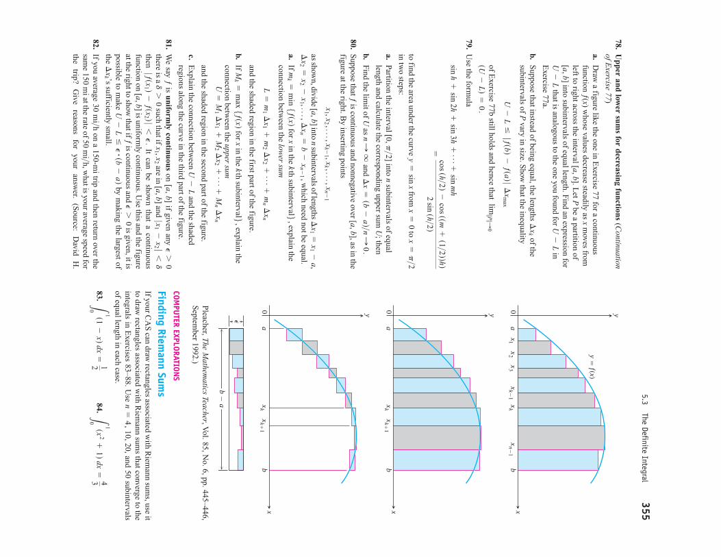
78.U
pper and lower sum
s for decreasing functions(C
ontinuationof E
xercise 77)
a.D
raw a figure like the one in E
xercise 77 for a continuousfunction ƒ(x) w
hose values decrease steadily as xm
oves fromleft to right across the interval [a,b]. L
et Pbe a partition of
[a,b] into subintervals of equal length. Find an expression forthat is analogous to the one you found for
inE
xercise 77a.
b.S
uppose that instead of being equal, the lengths of the
subintervals of Pvary in size. S
how that the inequality
of Exercise 77b still holds and hence that
79.U
se the formula
to find the area under the curve from
to
in two steps:
a.Partition the interval
into nsubintervals of equal
length and calculate the corresponding upper sum U
; then
b.Find the lim
it of Uas
and
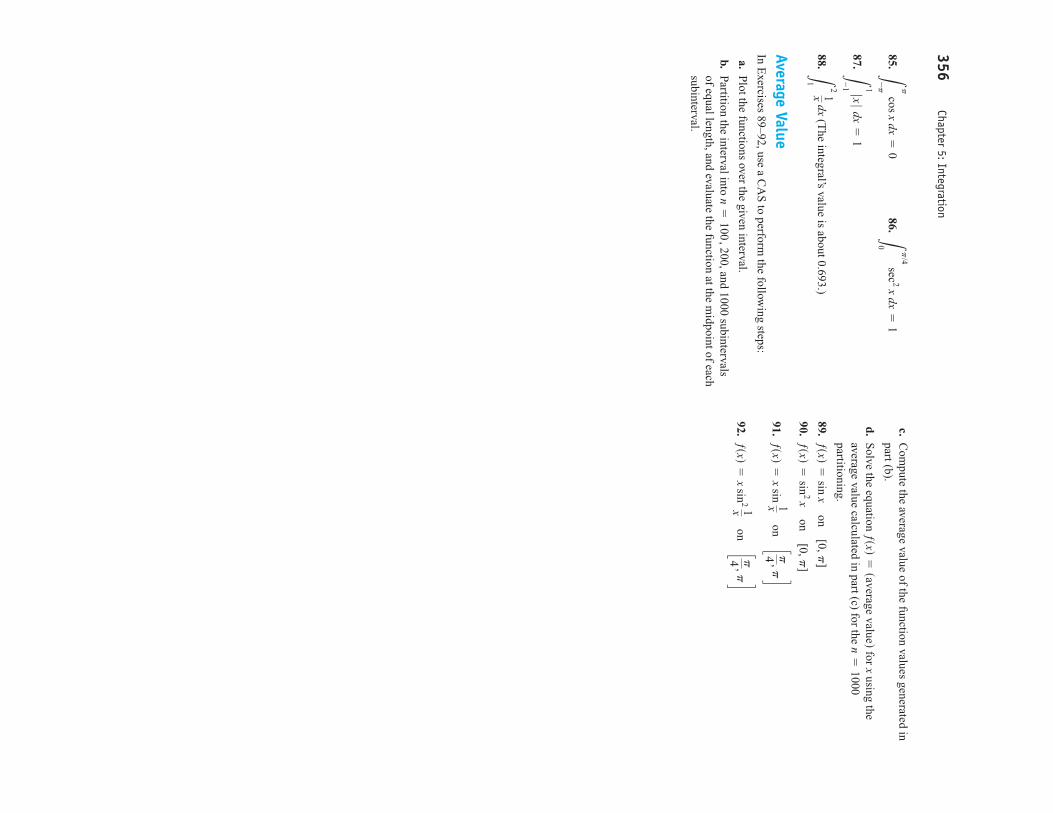
80.S
uppose that ƒis continuous and nonnegative over [a,b], as in the
figure at the right. By inserting points
asshow
n,divide[a,b]into
nsubintervals
oflengthsw
hich need not be equal.
a.If
explain theconnection betw
een the lower sum
and the shaded region in the first part of the figure.
b.If
explain theconnection betw
een the upper sum
and the shaded region in the second part of the figure.
c.E
xplain the connection between
and the shadedregions along the curve in the third part of the figure.
81.W
e say ƒis uniform
ly continuouson [a,
b] if given any there is a
such that if are in [a,b] and
then It can be show
n that a continuousfunction on [a,b] is uniform
ly continuous. Use this and the figure
at the right to show that if ƒ
is continuous and is given, it is
possible to make
by making the largest of
the sufficiently sm
all.
82.If you average 30 m
ih on a 150-m
i trip and then return over thesam
e 150 mi at the rate of 50 m
ih, w
hat is your average speed forthe
trip? G
ive reasons
for your
answer.
(Source:
David
H.
>>
¢x
k ’sU
-L
…P #sb
-ad
P7
0
ƒ ƒsx1 d
-ƒsx
2 dƒ6
P.
ƒ x1-
x2 ƒ
6d
x1 , x
2d
70
P7
0
U-
L
U=
M1 ¢
x1+
M2 ¢
x2+
Á+
Mn ¢
xn
Mk=
max
5ƒsxd for x in the k
th subinterval6,
L=
m1 ¢
x1+
m2 ¢
x2+
Á+
mn ¢
xn
mk=
min 5
ƒsxd for x in the kth subinterval6
,
¢x
2=
x2-
x1 ,Á
, ¢x
n=
b-
xn-
1 ,¢
x1=
x1-
a,
x1 , x
2 ,Á, x
k-1 , x
k ,Á, x
n-1
¢x
=sb
-ad>n:
0.
n:q
[0, p>2]x
=p>2
x=
0y
=sin
x
=cos sh>2d
-cos ssm
+s1>2ddhd
2 sin
sh>2dsin
h+
sin 2h
+sin
3h+
Á+
sin m
h
sU-
Ld=
0.
limƒƒ Pƒƒ :
0
U-
L…
ƒ ƒsbd-
ƒsadƒ ¢x
max
¢x
k
U-
LU
-L
Pleacher, T
he Mathem
atics Teacher, Vol. 85, N
o. 6, pp. 445–446,S
eptember 1992.)
COMPU
TER EXPLORATIONS
Finding Riemann Sum
sIf your C
AS
can draw rectangles associated w
ith Riem
ann sums, use it
to draw rectangles associated w
ith Riem
ann sums that converge to the
integrals in Exercises 83–88. U
se 10, 20, and 50 subintervals
of equal length in each case.
83.84.L
1
0sx
2+
1d dx=
43L
1
0s1
-xd dx
=12
n=
4,
5.3The Definite Integral
355x
y0a
bx
1x
2x
3xk�
1xn�
1xk
y � f(x)
x
y0a
bxk�
1xk
x
y0a
bxk�
1xk
b � a
�
85.86.
87.
88.(T
he integral’s value is about 0.693.)
Average ValueIn E
xercises 89–92, use a CA
S to perform
the following steps:
a.P
lot the functions over the given interval.
b.Partition the interval into
200, and 1000 subintervalsof equal length, and evaluate the function at the m
idpoint of eachsubinterval.
n=
100,
L2
1 1x
dx
L1
-1 ƒ xƒ dx
=1
Lp
/4
0 sec
2 x dx=
1Lp
-p
cos x dx=
0c.
Com
pute the average value of the function values generated inpart (b).
d.S
olve the equation for x
using theaverage value calculated in part (c) for the partitioning.
89.
90.
91.
92.ƒsxd
=x sin
2 1x on c p4
, pdƒsxd
=x sin
1x on c p4
, pdƒsxd
=sin
2 x on
[0, p]
ƒsxd=
sin x
on [0, p
]
n=
1000ƒsxd
=saverage valued
356Chapter 5: Integration

356 Chapter 5: Integration
The Fundamental Theorem of Calculus
In this section we present the Fundamental Theorem of Calculus, which is the central the-orem of integral calculus. It connects integration and differentiation, enabling us to com-pute integrals using an antiderivative of the integrand function rather than by taking limitsof Riemann sums as we did in Section 5.3. Leibniz and Newton exploited this relationshipand started mathematical developments that fueled the scientific revolution for the next200 years.
Along the way, we present the integral version of the Mean Value Theorem, which is an-other important theorem of integral calculus and used to prove the Fundamental Theorem.
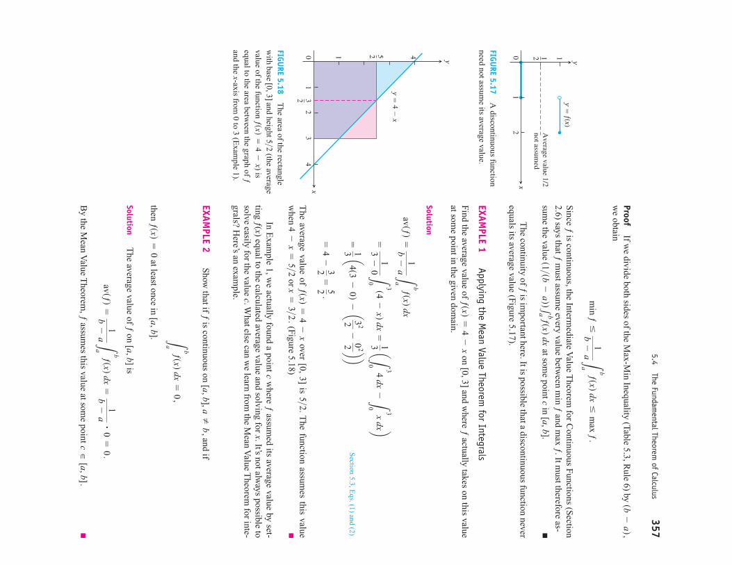
Mean Value Theorem for Definite Integrals
In the previous section, we defined the average value of a continuous function over aclosed interval [a, b] as the definite integral divided by the length or width
of the interval. The Mean Value Theorem for Definite Integrals asserts that this av-erage value is always taken on at least once by the function ƒ in the interval.
The graph in Figure 5.16 shows a positive continuous function defined overthe interval [a, b]. Geometrically, the Mean Value Theorem says that there is a number c in[a, b] such that the rectangle with height equal to the average value ƒ(c) of the functionand base width has exactly the same area as the region beneath the graph of ƒ froma to b.
b - a
y = ƒsxd
b - a1b
a ƒsxd dx
5.4
HISTORICAL BIOGRAPHY
Sir Isaac Newton(1642–1727)
y
xa b0 c
y � f (x)
f (c),
b � a
averageheight
FIGURE 5.16 The value ƒ(c) in theMean Value Theorem is, in a sense, theaverage (or mean) height of ƒ on [a, b].When the area of the rectangleis the area under the graph of ƒ from ato b,
ƒscdsb - ad = Lb
a ƒsxd dx .
ƒ Ú 0,
THEOREM 3 The Mean Value Theorem for Definite IntegralsIf ƒ is continuous on [a, b], then at some point c in [a, b],
ƒscd = 1b - a
Lb
aƒsxd dx .
ProofIf w
e divide both sides of the Max-M
in Inequality (Table 5.3, Rule 6) by
we obtain
Since ƒ
is continuous, the Intermediate V
alue Theorem
for Continuous F
unctions (Section
2.6) says that ƒm
ust assume every value betw
een min ƒ
and max ƒ. It m
ust therefore as-
sume the value
at some point c
in [a,b].
The continuity of ƒ
is important here. It is possible that a discontinuous function never
equals its average value (Figure5.17).
EXAMPLE 1
Applying the Mean Value Theorem
for Integrals
Find the average value of on [0, 3] and w
here ƒactually takes on this value
at some point in the given dom
ain.
Solution
Section 5.3, E
qs. (1) and (2)
The average value of
over [0, 3] is . T
he function assumes this value
when
or (Figure
5.18)
In Exam
ple 1, we actually found a point c
where ƒ
assumed its average value by set-
ting ƒ(x) equal to the calculated average value and solving for x. It’s not always possible to
solve easily for the value c. What else can w
e learn from the M
ean Value T
heorem for inte-
grals? Here’s an exam
ple.
EXAMPLE 2
Show
that if ƒis continuous on
and if
then at least once in [a,b].
SolutionT
he average value of ƒon [a,b] is
By the M
ean Value T
heorem, ƒ
assumes this value at som
e pointc H
[a, b].
avsƒd=
1b
-a
Lb
aƒsxd dx
=1
b-
a # 0
=0
.
ƒsxd=
0
Lb
aƒsxd dx
=0
,
[a, b], aZ
b,
x=
3>2.
4-
x=
5>25>2
ƒsxd=
4-
x
=4
-32
=52
.
=13
a4s3-
0d-a 3
22-
022 bb
=1
3-
0 L
3
0s4
-xd dx
=13
aL3
04 dx
-L3
0x dxb
avsƒd=
1b
-a
Lb
aƒsxd dx
ƒsxd=
4-
x
s1>sb-
add1baƒsxd dx
min
ƒ…
1b
-a
Lb
aƒsxd dx
…m
ax ƒ
.
sb-
ad,
5.4The Fundam
ental Theorem of Calculus
357
x
y
0 1
12 A
verage value 1/2not assum
ed
y � f(x)
12
FIGURE 5.17
A discontinuous function
need not assume its average value.
y � 4 �
x
52
32
y
x0
12
34
1 4
FIGURE 5.18
The area of the rectangle
with
base[0,3]and height
(the averagevalue of the function
) isequal to the area betw
een the graph of ƒand the x-axis from
0 to 3 (Exam
ple 1).
ƒsxd=
4-
x5>2
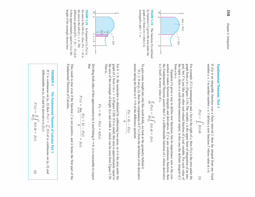
Fundamental Theorem
, Part 1
If ƒ(t) is an integrable function over a finite interval I, then the integral from any fixed
number
to another number
defines a new function F
whose value at x
is
(1)
For example, if ƒ
is nonnegative and xlies to the right of a, then F
(x) is the area under thegraph from
ato x
(Figure5.19). T
he variable xis the upper lim
it of integration of an inte-gral, but F
is just like any other real-valued function of a real variable. For each value ofthe input x, there is a w
ell-defined numerical output, in this case the definite integral of ƒ
from a
to x.E
quation (1) gives a way to define new
functions, but its importance now
is the con-nection it m
akes between integrals and derivatives. If ƒ
is any continuous function, thenthe F
undamental T
heorem asserts that F
is a differentiable function of xw
hose derivativeis ƒ
itself. At every value of x,
To gain some insight into w
hy this result holds, we look at the geom
etry behind it.If
on [a,b], then the computation of
from the definition of the derivative
means taking the lim
it as of the difference quotient
For the num
erator is obtained by subtracting two areas, so it is the area under the
graph of ƒfrom
xto
(Figure5.20). If h
is small, this area is approxim
ately equal tothe area of the rectangle of height ƒ(x) and w
idth h, which can be seen from
Figure 5.20.T
hat is,
Dividing both sides of this approxim
ation by hand letting
it is reasonable to expectthat
This result is true even if the function ƒ
is not positive, and it forms the first part of the
Fundam
ental Theorem
of Calculus.
F¿sxd=
limh:
0 Fsx+
hd-
Fsxdh
=ƒsxd.
h:0
,
Fsx+
hd-
FsxdL
hƒsxd.
x+
hh
70
,
Fsx+
hd-
Fsxdh
.
h:0
F¿sxdƒ
Ú0
ddx Fsxd
=ddxL
x
aƒstd dt
=ƒsxd.
Fsxd=L
x
aƒstd dt.
x H I
a H
I
358Chapter 5: Integration
t
y0a
xb
area � F
(x)y �
f(t)
FIGURE 5.19
The function F
(x) definedby E
quation (1) gives the area under thegraph of ƒ
from a
to xw
hen ƒis
nonnegative and x7
a.y �
f(t)
t
y0a
xx �
hb
f(x)
FIGURE 5.20
In Equation (1), F
(x) isthe area to the left of x. A
lso, is
the area to the left of T
hedifference quotient is then approxim
ately equal to ƒ(x), the
height of the rectangle shown here.
[Fsx+
hd-
Fsxd]>hx
+h
.Fsx
+hd
THEOREM
4The Fundam
ental Theorem of Calculus Part 1
If ƒis continuous on [a,
b] then is continuous on [a,
b] and
differentiable on and its derivative is
(2)F¿sxd
=ddxL
x
aƒstd dt
=ƒsxd.
ƒsxd;(a, b)
Fsxd=1
xa ƒstd dt

Before proving T
heorem 4, w
e look at several examples to gain a better understanding
of what it says.
EXAMPLE 3
Applying the Fundamental Theorem
Use the F
undamental T
heorem to find
(a)
(b)
(c)
(d)
Solution
(a)E
q. 2 with
(b)E
q. 2 with
(c)R
ule1
forintegralsin
Table5.3
ofSection
5.3sets
thisup
fortheF
undamentalT
heorem.
Rule 1
(d)T
he upper limit of integration is not x
but T
his makes y
a composite of the tw
ofunctions,
We m
ust therefore apply the Chain R
ule when finding
.
=2x cos x
2
=cossx
2d #2x =
cos u # dudx
=adduL
u
1 cos t dtb # dudx
dydx=
dydu # dudx
dy>dxy
=Lu
1 cos t dt
and u
=x
2.
x2.
=-
3x sin x
=-
ddxLx
53t sin
t dt
dydx=
ddx L
5
x3t sin
t dt=
ddx a-L
x
53t sin
t dtbƒstd
=1
1+
t 2
ddx L
x
0
11
+t 2 dt
=1
1+
x2
ƒ(t)=
cos tddx
Lx
a cos t dt
=cos x
dydx if
y=L
x2
1 cos t dt
dydx if
y=L
5
x3t sin
t dt
ddx L
x
0
11
+t 2 dt
ddx L
x
a cos t dt
5.4The Fundam
ental Theorem of Calculus
359
EXAMPLE 4
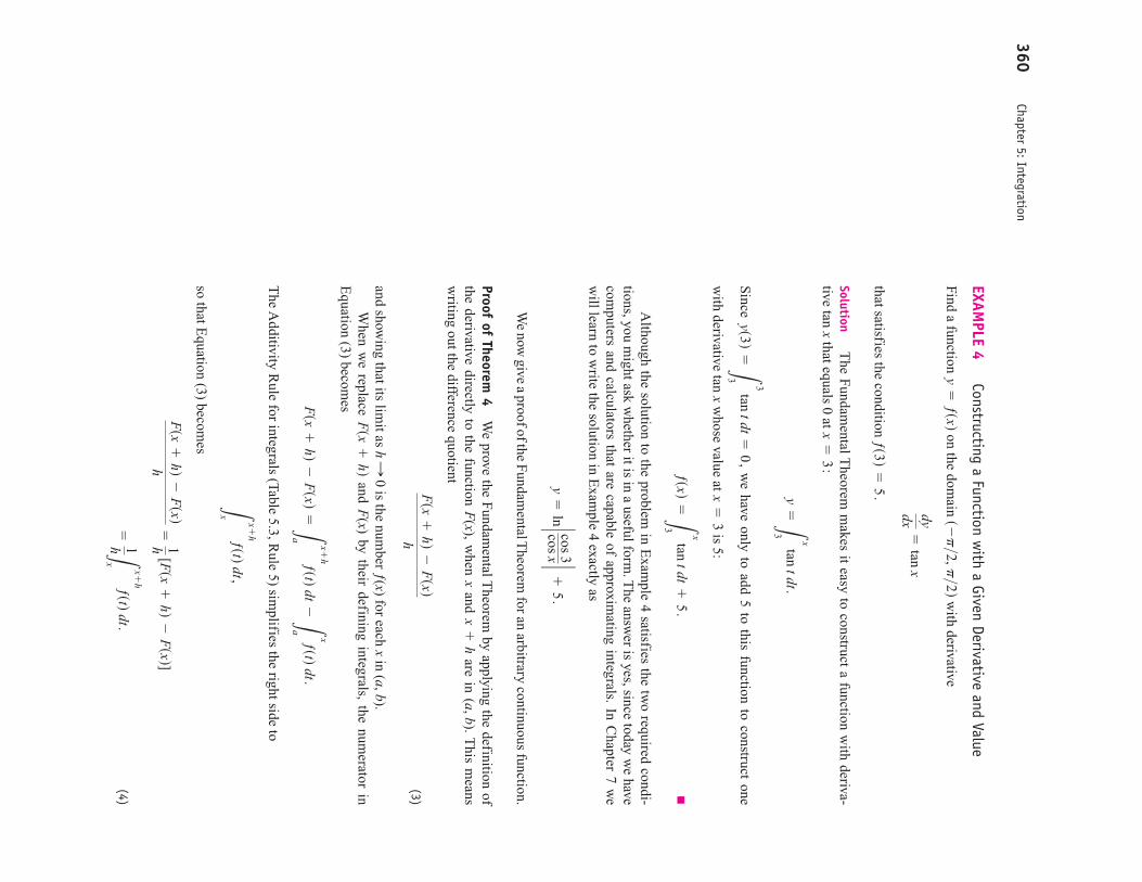
Constructing a Function with a Given Derivative and Value
Find a function on the dom
ain w
ith derivative
that satisfies the condition
SolutionT
he Fundam
ental Theorem
makes it easy to construct a function w
ith deriva-tive tan x
that equals 0 at
Since
we have only to add 5 to this function to construct one
with derivative tan x
whose value at
is 5:
Although the solution to the problem
in Exam
ple 4 satisfies the two required condi-
tions, you might ask w
hether it is in a useful form. T
he answer is yes, since today w
e havecom
puters and calculators that are capable of approximating integrals. In C
hapter 7w
ew
ill learn to write the solution in E
xample 4 exactly as
We
nowgive
aproofofthe
Fundam
entalTheorem
for an arbitrary continuous function.
Proof of Theorem 4
We prove the F
undamental T
heorem by applying the definition of
the derivative directly to the function F(x), w
hen xand
are in T
his means
writing out the difference quotient
(3)
and showing that its lim
it as is the num
ber ƒ(x) for each xin
.W
hen we replace
and F(x) by their defining integrals, the num
erator inE
quation (3) becomes
The A
dditivity Rule for integrals (Table 5.3, R
ule 5) simplifies the right side to
so that Equation (3) becom
es
(4) =
1hLx+
h
xƒstd dt.
Fsx+
hd-
Fsxdh
=1h
[Fsx+
hd-
Fsxd]
Lx+
h
xƒstd dt,
Fsx+
hd-
Fsxd=L
x+h
aƒstd dt
-Lx
aƒstd dt.
Fsx+
hd(a, b)
h:0
Fsx+
hd-
Fsxdh
(a, b).x
+h
y=
ln` cos 3cos x `
+5
.
ƒsxd=L
x
3 tan
t dt+
5.
x=
3
ys3d=L
3
3 tan
t dt=
0,
y=L
x
3 tan
t dt.
x=
3:
ƒs3d=
5.
dydx=
tan x
s-p>2, p>2d
y=
ƒsxd
360Chapter 5: Integration
According to the M
ean Value T
heorem for D
efinite Integrals, the value of the last ex-pression in E
quation (4) is one of the values taken on by ƒin the interval betw
een xand
That is, for som
e number c
in this interval,
(5)
As
approaches x, forcing cto approach x
also (because cis trapped betw
eenx
and ). S
ince ƒis continuous at x, ƒ(c) approaches ƒ(x):
(6)
Going back to the beginning, then, w
e have
Definition of derivative
Eq. (4)
Eq. (5)
Eq. (6)
If then the lim
it of Equation (3) is interpreted as a one-sided lim
it with
or , respectively. T
hen Theorem
1 in Section 3.1 show
s that Fis continuous for
every point of [a, b]. This concludes the proof.
Fundamental Theorem
, Part 2 (The Evaluation Theorem)
We now
come to the second part of the F
undamental T
heorem of C
alculus. This part
describes how to evaluate definite integrals w
ithout having to calculate limits of R
iemann
sums. Instead w
e find and evaluate an antiderivative at the upper and lower lim
its ofintegration.
h:0
-h:
0+
x=
a or b,
=ƒsxd.
=limh:
0 ƒscd
=limh:
0 1hLx+
h
xƒstd dt
dFdx=
limh:
0 Fsx+
hd-
Fsxdh
limh:
0 ƒscd=
ƒsxd.
x+
hh:
0, x+
h
1hLx+
h
xƒstd dt
=ƒscd.
x+
h.
5.4The Fundam
ental Theorem of Calculus
361
THEOREM
4 (Continued)The Fundam
ental Theorem of Calculus Part 2
If ƒis continuous at every point of [a,b] and F
is any antiderivative of ƒ on [a,b],then
Lb
aƒsxd dx
=Fsbd
-Fsad.
ProofPart 1 of the Fundam
ental Theorem
tells us that an antiderivative of ƒexists, nam
ely
Thus, if F
is anyantiderivative of ƒ, then
for some constant C
for(by C
orollary 2 of the Mean V
alue Theorem
for Derivatives, S
ection 4.2).S
ince both Fand G
are continuous on [a, b], we see that
also holdsw
hen and
by taking one-sided limits (as
and x:b
-d.x:
a+
x=
bx
=a
F(x)
=G
(x)+
Ca
6x
6b
Fsxd=
Gsxd
+C
Gsxd
=Lx
aƒstd dt.

Evaluating
we have
The theorem
says that to calculate the definite integral of ƒover [a,b] all w
e need todo is:
1.Find an antiderivative F
of ƒ, and
2.C
alculate the number
The usual notation for
is
depending on whether F
has one or more term
s.
EXAMPLE 5
Evaluating Integrals
(a)
(b)
(c)
The process used in E
xample 5 w
as much easier than a R
iemann sum
computation.
The conclusions of the F
undamental T
heorem tell us several things. E
quation (2) canbe rew
ritten as
which says that if you first integrate the function ƒ
and then differentiate the result, you getthe function ƒ
back again. Likew
ise, the equation
says that if you first differentiate the function Fand then integrate the result, you get the
function Fback (adjusted by an integration constant). In a sense, the processes of integra-
Lx
a dFdt
dt=L
x
aƒstd dt
=Fsxd
-Fsad
ddxLx
aƒstd dt
=dFdx
=ƒsxd,
=[8
+1]
-[5]
=4
.
=cs4d 3/2+
44 d-cs1d 3/2
+41 d
L4
1 a 32 1
x-
4x2 b
dx=cx
3/2+
4x d1 4
L0
-p>4 sec x tan
x dx=
sec xd-p
/4
0
=sec 0
-sec a-
p4 b=
1-2
2
Lp
0 cos x dx
=sin
xd0 p
=sin
p-
sin 0
=0
-0
=0
Fsxdda b or
cFsxdda b,
Fsbd-
Fsad1
ba ƒsxd dx
=Fsbd
-Fsad.
=Lb
aƒstd dt.
=Lb
aƒstd dt
-0
=Lb
aƒstd dt
-La
aƒstd dt
=Gsbd
-Gsad
Fsbd-
Fsad=
[Gsbd
+C
]-
[Gsad
+C
]
Fsbd-
Fsad,
362Chapter 5: Integration
tion and differentiation are “inverses” of each other. The F
undamental T
heorem also says
that every continuous function ƒhas an antiderivative F
. And it says that the differential
equation has a solution (nam
ely, the function )
for every continu-ous function ƒ.
Total Area
The R
iemann sum
contains terms such as
which give the area of a rectangle w
henis positive. W
hen is negative, then the product
is the negative of therectangle’s area. W
hen we add up such term
s for a negative function we get the negative of
the area between the curve and the x-axis. If w
e then take the absolute value, we obtain the
correct positive area.
EXAMPLE 6
Finding Area Using Antiderivatives
Calculate the area bounded by the x-axis and the parabola
SolutionW
e find where the curve crosses the x-axis by setting
which gives
The curve is sketched in Figure
5.21, and is nonnegative on T
he area is
The curve in Figure 5.21
is an arch of a parabola, and it is interesting to note that the areaunder such an arch is exactly equal to tw
o-thirds the base times the altitude:
To compute the area of the region bounded by the graph of a function
andthe x-axis requires m
ore care when the function takes on both positive and negative values.
We m
ust be careful to break up the interval [a,b] into subintervals on which the function
doesn’t change sign. Otherw
ise we m
ight get cancellation between positive and negative
signed areas, leading to an incorrect total. The correct total area is obtained by adding the
absolute value of the definite integral over each subinterval where ƒ(x) does not change
sign. The term
“area” will be taken to m
ean total area.
EXAMPLE 7
Canceling Areas
Figure5.22
shows the graph of the function
between
and C
ompute
(a)the definite integral of ƒ(x) over
(b)the area betw
een the graph of ƒ(x) and the x-axis over [0, 2p
].
[0, 2p
].
x=
2p
.x
=0
ƒsxd=
sin x
y=
ƒsxd
23 s5da 254 b=
1256=
20 56 .
=a12-
2-
83 b-a-
18-
92+
273 b=
20 56 .
L2
-3 s6
-x
-x
2d dx=c6x
-x
22-
x33 d-
3
2
[-3, 2].
x=
-3
or x
=2
.
y=
0=
6-
x-
x2=s3
+xds2
-xd,
y=
6-
x-
x2.
ƒsck d ¢
kƒsc
k dƒsc
k dƒsc
k d ¢k
y=
F(x)
dy>dx=
ƒsxd
5.4The Fundam
ental Theorem of Calculus
363
–3–2
–10
12
x
y
y � 6 �
x � x
2
254
FIGURE 5.21
The area of this
parabolic arch is calculated with a
definite integral (Exam
ple 6).
–1 0 1
x
y
�2�
y � sin x
Area �
2
Area �
�–2� � 2
FIGURE 5.22
The total area betw
eenand
the x-axis for is the sum
of the absolute values of two
integrals (Exam
ple 7).
0…
x…
2p
y=
sin x
SolutionT
he definite integral for is given by
The definite integral is zero because the portions of the graph above and below
the x-axism
ake canceling contributions.T
he area between the graph of ƒ(x) and the x-axis over
is calculated by break-ing up the dom
ain of sin xinto tw
o pieces: the interval over w
hich it is nonnegativeand the interval
over which it is nonpositive.
The second integral gives a negative value. T
he area between the graph and the axis is ob-
tained by adding the absolute values
Area
=ƒ 2
ƒ +ƒ -
2ƒ=
4.
L2p
p
sin x dx
=-
cos xdp 2p
=-
[cos 2p
-cos p
]=
-[1
-s-
1d]=
-2
.
Lp
0 sin
x dx=
-cos xd0 p
=-
[cos p-
cos 0]=
-[-
1-
1]=
2.
[p, 2p
][0, p
] [0, 2p
]
L2p
0 sin
x dx=
-cos xd0 2
p
=-
[cos 2p
-cos 0]
=-
[1-
1]=
0.
ƒsxd=
sin x
364Chapter 5: Integration
x
y02
–1
y � x
3 � x
2 � 2x
Area ��
83– ⎢⎢
⎢⎢83
Area �
512
FIGURE 5.23
The region betw
een thecurve
and the x-axis(E
xample 8).y
=x
3-
x2-
2x
Summ
ary:To find the area betw
een the graph of and the x-axis over the interval
[a,b], do the following:
1.S
ubdivide [a,b] at the zeros of ƒ.
2.Integrate ƒ
over each subinterval.
3.A
dd the absolute values of the integrals.
y=
ƒsxd
EXAMPLE 8
Finding Area Using Antiderivatives
Find the area of the region between the x-axis and the graph of
SolutionFirst find the zeros of ƒ. S
ince
the zeros are and 2 (Figure
5.23). The zeros subdivide
into two subin-
tervals: on w
hich and [0,2], on w
hich W
e integrate ƒover each
subinterval and add the absolute values of the calculated integrals.
The total enclosed area is obtained by adding the absolute values of the calculated integrals,
Total enclosed area
=512
+`-83 `
=3712
.
L2
0sx
3-
x2-
2xd dx=c x
44-
x33
-x
2d0 2
=c4-
83-
4d-
0=
-83
L0
-1 sx
3-
x2-
2xd dx=c x
44-
x33
-x
2d-1
0
=0
-c 14+
13-
1d=
512
ƒ…
0.
ƒÚ
0,
[-1, 0],
[-1, 2]
x=
0, -1
,
ƒsxd=
x3-
x2-
2x=
xsx2-
x-
2d=
xsx+
1dsx-
2d,
-1
…x
…2
.ƒ(x)
=x
3-
x2-
2x,
5.4The Fundam
ental Theorem of Calculus
365
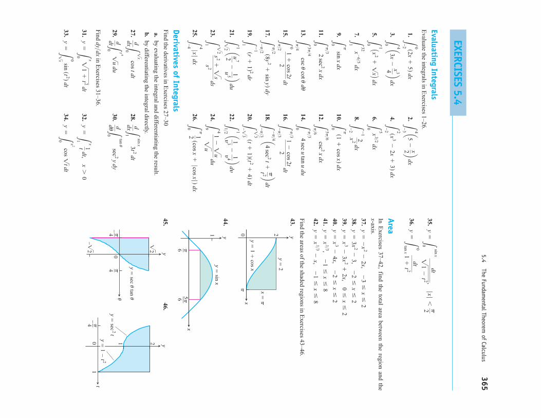
EXERCISES 5.4
Evaluating IntegralsE
valuate the integrals in Exercises 1–26.
1.2.
3.4.
5.6.
7.8.
9.10.
11.12.
13.14.
15.16.
17.18.
19.20.
21.22.
23.24.
25.26.
Derivatives of IntegralsFind the derivatives in E
xercises 27–30
a.by evaluating the integral and differentiating the result.
b.by differentiating the integral directly.
27.28.
29.30.
Find in E
xercises 31–36.
31.32.
33.34.
y=L
x2
0 cos 1
t dty
=L0
1x sin
st 2d dt
y=L
x
1 1t dt,
x7
0y
=Lx
0 21
+t 2 dt
dy>dxdduL
tan u
0 sec
2 y dyddtL
t4
0 1u du
ddxL sin
x
13t 2 dt
ddxL1
x
0 cos t dt
Lp
0 12
scos x+
ƒ cos xƒ d dxL
4
-4 ƒ xƒ dx
L4
9 1
-2u
2u
duL2
2
1 s
2+2
s
s2
ds
L1
1>2 a1y3
-1y4 b
dy
L1
22 a u
72-
1u5 b
du
L2
3
-23 st
+1dst 2
+4d dt
L-
1
1sr
+1d 2 dr
L-p>4
-p>3 a4
sec2 t
+pt 2 b
dtLp>2-p>2 s8y
2+
sin yd dy
Lp>3-p>3 1
-cos 2t2
dtL
0
p>2 1+
cos 2t2
dt
Lp>30
4 sec u
tan u du
L3p>4
p>4 csc u cot u d
u
L5p>6
p>6 csc
2 x dxLp>30
2 sec
2 x dx
Lp
0s1
+cos xd dx
Lp
0 sin
x dx
L-
1
-2
2x2 dx
L32
1x-
6>5 dx
L5
0x
3>2 dxL
1
0 A x2+1
xB dxL
2
-2 sx
3-
2x+
3d dxL
4
0 a3x-
x34 b
dx
L4
-3 a5
-x2 b
dxL
0
-2 s2x
+5d dx
35.
36.
AreaIn E
xercises 37–42, find the total area between the region and the
x-axis.
37.
38.
39.
40.
41.
42.
Find the areas of the shaded regions in Exercises 43–46.
43.
44.
45.46.
t
y
�4–
01
1 2
y � sec
2 t
y � 1 �
t 2
�
y
–�2
�2
�4�4
–0
y � sec � tan �
y
x
1
�65�6
y � sin x
x
y0 2
�
y � 2
x � �
y � 1 �
cos x
y=
x1>3
-x,
-1
…x
…8
y=
x1>3,
-1
…x
…8
y=
x3-
4x, -
2…
x…
2
y=
x3-
3x2+
2x, 0
…x
…2
y=
3x2-
3, -
2…
x…
2
y=
-x
2-
2x, -
3…
x…
2
y=L
0
tan x
dt
1+
t 2
y=L
sin x
0
dt
21
-t 2 ,
ƒ xƒ6p2

Initial Value Problems
Each of the follow
ing functions solves one of the initial value prob-lem
s in Exercises 47–50. W
hich function solves which problem
? Give
brief reasons for your answers.
a.b.
c.d.
47.48.
49.50.
Express the solutions of the initial value problem
s in Exercises 51–54
in terms of integrals.
51.
52.
53.
54.
Applications55.
Archim
edes’area
formula
for parabolas
Archim
edes(287–212
B.C.), inventor, military engineer, physicist, and the
greatestmathem
aticianofclassicaltim
esin
theW
esternw
orld,dis-covered that the area under a parabolic arch is tw
o-thirds the basetim
es the height. Sketch the parabolic arch assum
ing that hand b
are positive. Then use
calculus to find the area of the region enclosed between the arch
and the x-axis.
56.R
evenue from m
arginal revenueS
uppose that a company’s
marginal revenue from
the manufacture and sale of egg beaters is
where r
is measured in thousands of dollars and x
in thousands ofunits. H
ow m
uch money should the com
pany expect from a pro-
duction run of thousand egg beaters? To find out, integrate
the marginal revenue from
to
57.C
ost from m
arginal costT
he marginal cost of printing a poster
when x
posters have been printed is
dollars. Find the cost of printing posters 2–100.
58.(C
ontinuation of Exercise 57.) Find
the cost ofprinting posters 101–400.
cs400d-
cs100d,cs100d
-cs1d,
dcdx=
121
x
x=
3.
x=
0x
=3 drdx
=2
-2>sx
+1d 2,
-b>2
…x
…b>2
,y
=h
-s4h>b
2dx2,
dydt
=gstd,
yst0 d=y
0
dsdt=
ƒstd, sst0 d
=s
0
dydx=2
1+
x2,
ys1d=
-2
dydx=
sec x, ys2d
=3
y¿=
1x , ys1d
=-
3y¿
=sec x,
ys0d=
4
y¿=
sec x, ys-
1d=
4dydx
=1x ,
yspd=
-3
y=L
x
p
1t dt-
3y
=Lx
-1 sec t dt
+4
y=L
x
0 sec t dt
+4
y=L
x
1 1t dt
-3
Drawing Conclusions About M
otion from Graphs
59.S
uppose that ƒis the differentiable function show
n in the accom-
panying graph and that the position at time t
(sec) of a particlem
oving along a coordinate axis is
meters. U
se the graph to answer the follow
ing questions. Give
reasons for your answers.
a.W
hat is the particle’s velocity at time
b.Is the acceleration of the particle at tim
e positive, or
negative?
c.W
hat is the particle’s position at time
d.A
t what tim
e during the first 9 sec does shave its largest
value?
e.A
pproximately w
hen is the acceleration zero?
f.W
hen is the particle moving tow
ard the origin? away from
theorigin?
g.O
n which side of the origin does the particle lie at tim
e
60.S
uppose that gis the differentiable function graphed here and that
the position at time t(sec) of a particle m
oving along a coordinateaxis is
meters. U
se the graph to answer the follow
ing questions. Give
reasons for your answers.
x
y
36
9
2 4 6 8–2
–4–6
y � g(x) (6, 6)
(7, 6.5)
s=L
t
0gsxd dx
t=
9?
t=
3?
t=
5
t=
5?
y
x0
12
34
56
78
9
1 2 3 4–1–2
(1, 1)
(2, 2)(5, 2)
(3, 3)
y � f(x)
s=L
t
0ƒsxd dx
366Chapter 5: Integration

a.W
hat is the particle’s velocity at
b.Is the acceleration at tim
e positive, or negative?
c.W
hat is the particle’s position at time
d.W
hen does the particle pass through the origin?
e.W
hen is the acceleration zero?
f.W
hen is the particle moving aw
ay from the origin? tow
ard theorigin?
g.O
n which side of the origin does the particle lie at
Theory and Examples
61.S
how that if k
is a positive constant, then the area between the
x-axis and one arch of the curve is
.
62.Find
63.S
uppose Find ƒ(x).
64.Find ƒ(4) if
65.Find the linearization of
at
66.Find the linearization of
at
67.S
uppose that ƒhas a positive derivative for all values of x
and thatW
hich of the following statem
ents must be true of the
function
Give reasons for your answ
ers.
a.g
is a differentiable function of x.
b.g
is a continuous function of x.
c.T
he graph of ghas a horizontal tangent at
d.g
has a local maxim
um at
e.g
has a local minim
um at
f.T
he graph of ghas an inflection point at
g.T
he graph of crosses the x-axis at
68.S
uppose that ƒhas a negative derivative for all values of x
andthat
Which of the follow
ing statements m
ust be true ofthe function
hsxd=L
x
0 ƒstd dt?
ƒs1d=
0.
x=
1.
dg>dxx
=1
.
x=
1.
x=
1.
x=
1.
gsxd=L
x
0 ƒstd dt?
ƒs1d=
0.
x=
-1
.
gsxd=
3+L
x2
1 sec st
-1d dt
x=
1.
ƒsxd=
2-L
x+1
2
91
+t dt
1x0 ƒstd dt
=x cos p
x.
1x1 ƒstd dt
=x
2-
2x+
1.
limx:
0 1x3 L
x
0
t 2
t 4+
1 dt.
2>ky
=sin
kx
t=
9?
t=
3?
t=
3
t=
3?
Give reasons for your answ
ers.
a.h
is a twice-differentiable function of x.
b.h
and are both continuous.
c.T
he graph of hhas a horizontal tangent at
d.h
has a local maxim
um at
e.h
has a local minim
um at
f.T
he graph of hhas an inflection point at
g.T
he graph of crosses the x-axis at
69.T
he Fundam
ental Theorem
If ƒis continuous, w
e expect
to equal ƒ(x), as in the proof of Part 1 of the Fundam
ental Theo-
rem. For instance, if
then
(7)
The right-hand side of E
quation (7) is the difference quotient forthe derivative of the sine, and w
e expect its limit as
to becos x.G
raph cos xfor
Then, in a different color if
possible, graph the right-hand side of Equation (7) as a function
of xfor
and 0.1. Watch how
the latter curves con-verge to the graph of the cosine as
70.R
epeat Exercise 69 for
What is
Graph
for T
hen graph the quotientas a function of x
for and 0.1.
Watch how
the latter curves converge to the graph of as
COMPU
TER EXPLORATIONS
In Exercises 71–74, let
for the specified function ƒand interval [a,b]. U
se a CA
S to perform
the following steps and an-
swer the questions posed.
a.P
lot the functions ƒand F
together over [a,b].
b.S
olve the equation W
hat can you see to be true aboutthe graphs of ƒ
and Fat points w
here Is your
observation borne out by Part 1 of the Fundam
ental Theorem
coupled with inform
ation provided by the first derivative?E
xplain your answer.
c.O
ver what intervals (approxim
ately) is the function Fincreasing
and decreasing? What is true about ƒ
over those intervals?
d.C
alculate the derivative and plot it together w
ith F. W
hat canyou see to be true about the graph of F
at points where
Is your observation borne out by Part 1 of theF
undamental T
heorem? E
xplain your answer.
ƒ¿sxd=
0?
ƒ¿
F¿sxd=
0?
F¿sxd=
0.
Fsxd=1
xa ƒstd dt
h:0
.3x
2h
=1, 0.5, 0.2
,ssx
+hd 3
-x
3d>h-
1…
x…
1.
ƒsxd=
3x2
limh:
0 1h L
x+h
x 3t 2 dt
=limh:
0 sx+
hd 3-
x3
h?
ƒstd=
3t 2. h:0
.h
=2, 1, 0.5
, -p
…x
…2p
.
h:0
1h L
x+h
x cos t dt
=sin
sx+
hd-
sin x
h.
ƒstd=
cos t,
limh:
0 1h L
x+h
xƒstd dt
x=
1.
dh>dxx
=1
.
x=
1.
x=
1.
x=
1.
dh>dx 5.4The Fundam
ental Theorem of Calculus
367
TT

71.
72.
73.
74.
In Exercises 75–78, let
for the specified a,u, andƒ. U
se a CA
S to perform
the following steps and answ
er the questionsposed.
a.Find the dom
ain of F.
b.C
alculate and determ
ine its zeros. For what points in its
domain is F
increasing? decreasing?
c.C
alculate and determ
ine its zero. Identify the localextrem
a and the points of inflection of F.
F–sxd
F¿sxd
Fsxd=1
u(x)a
ƒstd dt
ƒsxd=
x cos px,
[0, 2p
]
ƒsxd=
sin 2x cos x3
, [0, 2p
]
ƒsxd=
2x4-
17x3+
46x2-
43x+
12, c0, 92 dƒsxd
=x
3-
4x2+
3x, [0, 4]
d.U
sing the information from
parts (a)–(c), draw a rough hand-
sketch of over its dom
ain. Then graph F
(x) on yourC
AS
to support your sketch.
75.
76.
77.
78.
In Exercises 79 and 80, assum
e that fis continuous and u(x) is tw
ice-differentiable.
79.C
alculate and check your answ
er using a CA
S.
80.C
alculate and check your answ
er using a CA
S.
d2
dx2L
usxd
aƒstd dt
ddxLusxd
aƒstd dt
a=
0, usxd
=1
-x
2, ƒsxd
=x
2-
2x-
3
a=
0, usxd
=1
-x,
ƒsxd=
x2-
2x-
3
a=
0, usxd
=x
2, ƒsxd
=21
-x
2
a=
1, usxd
=x
2, ƒsxd
=21
-x
2
y=
Fsxd
368Chapter 5: Integration
368 Chapter 5: Integration
Indefinite Integrals and the Substitution Rule
A definite integral is a number defined by taking the limit of Riemann sums associatedwith partitions of a finite closed interval whose norms go to zero. The Fundamental Theo-rem of Calculus says that a definite integral of a continuous function can be computed eas-ily if we can find an antiderivative of the function. Antiderivatives generally turn out to bemore difficult to find than derivatives. However, it is well worth the effort to learn tech-niques for computing them.
Recall from Section 4.8 that the set of all antiderivatives of the function ƒ is called theindefinite integral of ƒ with respect to x, and is symbolized by
The connection between antiderivatives and the definite integral stated in the FundamentalTheorem now explains this notation. When finding the indefinite integral of a function ƒ,remember that it always includes an arbitrary constant C.
We must distinguish carefully between definite and indefinite integrals. A definite in-
tegral is a number. An indefinite integral is a function plus an arbi-trary constant C.
So far, we have only been able to find antiderivatives of functions that are clearly rec-ognizable as derivatives. In this section we begin to develop more general techniques forfinding antiderivatives. The first integration techniques we develop are obtained by invert-ing rules for finding derivatives, such as the Power Rule and the Chain Rule.
The Power Rule in Integral Form
If u is a differentiable function of x and n is a rational number different from theChain Rule tells us that
ddx
a un+1
n + 1b = un
dudx
.
-1,
1ƒsxd dx1ba ƒsxd dx
Lƒsxd dx .
5.5
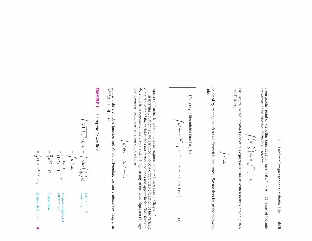
From another point of view
, this same equation says that
is one of the anti-derivatives of the function
Therefore,
The integral on the left-hand side of this equation is usually w
ritten in the simpler “differ-
ential” form,
obtained by treating the dx’s as differentials that cancel. We are thus led to the follow
ingrule.
Lu
n du,
L aun dudx b
dx=
un+
1
n+
1+
C.
unsdu>dxd.
un+
1>sn+
1d
5.5Indefinite Integrals and the Substitution Rule
369
If uis any differentiable function, then
(1)L
un du
=u
n+1
n+
1+
C sn
Z-
1, n rationald.
Equation (1) actually holds for any real exponent
as we see in C
hapter 7.In deriving E
quation (1), we assum
ed uto be a differentiable function of the variable
x, but the name of the variable does not m
atter and does not appear in the final formula.
We could have represented the variable w
ith or any other letter. E
quation (1) saysthat w
henever we can cast an integral in the form
with u
a differentiable function and duits differential, w
e can evaluate the integral as
EXAMPLE 1
Using the Power Rule
Sim
pler form
Replace u
by 1+
y2.
=23
s1+
y2d 3>2
+C
=23
u3>2
+C
=us1>2d+
1
s1>2d+
1+
C
=Lu
1>2 du
L 21
+y
2#2y dy=L 1
u #a dudy b dy
[un+
1>sn+
1d]+
C.
Lu
n du, sn
Z-
1d,
u, t, y,
nZ
-1,
Let
du>dy=
2yu
=1
+y
2,
Integrate, using Eq. (1)
with n
=1>2
.
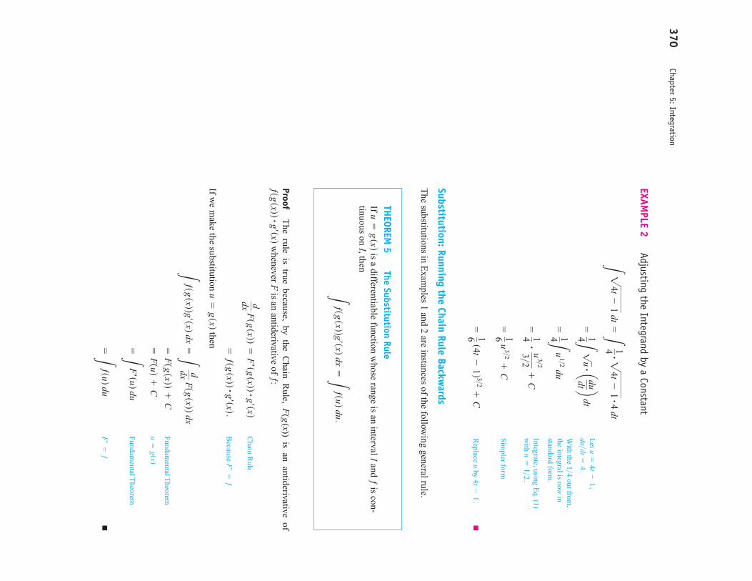
EXAMPLE 2
Adjusting the Integrand by a Constant
Sim
pler form
Replace u
by
Substitution: Running the Chain Rule Backwards
The substitutions in E
xamples 1 and 2 are instances of the follow
ing general rule.
4t-
1.
=16
s4t-
1d 3>2+
C
=16
u3>2
+C
=14
# u3>23>2
+C
=14L
u1>2 du
=14L 1
u #a dudt b dt
L 24t
-1 dt
=L 14 #2
4t-
1 #4 dt
370Chapter 5: Integration
Let
du>dt=
4.
u=
4t-
1,
With the
out front,the integral is now
instandard form
.
1>4Integrate, using E
q. (1)w
ith n=
1>2.
THEOREM
5The Substitution Rule
If is a differentiable function w
hose range is an interval Iand ƒ
is con-tinuous on I, then
Lƒsgsxddg¿sxd dx
=Lƒsud du
.
u=
gsxd
ProofT
he rule is true because, by the Chain R
ule, F(g
(x)) is an antiderivative ofw
henever Fis an antiderivative of ƒ:
Chain R
ule
Because
If we m
ake the substitution then
Fundam
ental Theorem
Fundam
ental Theorem
F¿=
ƒ =L
ƒsud du
=LF¿sud du
u=
gsxd =
Fsud+
C
=Fsgsxdd
+C
Lƒsgsxddg¿sxd dx
=L ddx
Fsgsxdd dx
u=
gsxd
F¿=
ƒ =
ƒsgsxdd #g¿sxd. ddx
Fsgsxdd=
F¿sgsxdd #g¿sxdƒsgsxdd #g¿sxd
The S
ubstitution Rule provides the follow
ing method to evaluate the integral
when ƒ
and are continuous functions:
1.S
ubstitute and
to obtain the integral
2.Integrate w
ith respect to u.
3.R
eplace uby g
(x) in the result.
EXAMPLE 3
Using Substitution
Replace u
by
We can verify this solution by differentiating and checking that w
e obtain the originalfunction
EXAMPLE 4
Using Substitution
Integrate with respect to u.
Replace u
by x3.
=-
13 cos sx
3d+
C
=13
s-cos ud
+C
=13L
sin u du
=L sin
u # 13 du
Lx
2 sin sx
3d dx=L
sin sx
3d #x2 dx
cos s7u
+5d.
7u
+5
. =
17 sin
s7u
+5d
+C
=17
sin u
+C
=17L
cos u du
L cos s7
u+
5d du
=L cos u # 17
du
Lƒsud du
.
du=
g¿sxd dxu
=gsxd
g¿
Lƒsgsxddg¿sxd dx,
5.5Indefinite Integrals and the Substitution Rule
371
s1>7d du=
du
.L
et u=
7u
+5, du
=7 du,
With the (
) out front, theintegral is now
in standard form.
1>7Integrate w
ith respect to u,Table 4.2.
s1>3d du=
x2 dx
.
du=
3x2 dx,
Let u
=x
3,
EXAMPLE 5
Using Identities and Substitution
The success of the substitution m
ethod depends on finding a substitution that changesan integral w
e cannot evaluate directly into one that we can. If the first substitution fails,
try to simplify the integrand further w
ith an additional substitution or two (see E
xercises49 and 50). A
lternatively, we can start fresh. T
here can be more than one good w
ay to start,as in the next exam
ple.
EXAMPLE 6
Using Different Substitutions
Evaluate
SolutionW
e can use the substitution method of integration as an exploratory tool: S
ub-stitute for the m
ost troublesome part of the integrand and see how
things work out. For the
integral here, we m
ight try or w
e might even press our luck and take u
to bethe entire cube root. H
ere is what happens in each case.
Solution 1:S
ubstitute
In the form
Integrate with respect to u.
Replace u
by z2+
1.
=32
sz2+
1d 2>3+
C
=32
u2>3
+C
=u
2>32>3+
C
1u
n du =L
u-
1>3 du
L
2z dz
23
z2+
1=L
du
u1>3
u=
z2+
1.
u=
z2+
1 L
2z dz
23
z2+
1 .
u=
2x =
12 tan
2x+
C
ddu tan
u=
sec2 u
=12
tan u
+C
=12L
sec2 u du
=Lsec
2 u # 12 du
1cos 2x
=sec 2x
L
1cos
2 2x dx
=Lsec
2 2x dx
372Chapter 5: Integration
dx=s1>2d du
du=
2 dx,u
=2x,
Let
du=
2z dz.u
=z
2+
1,
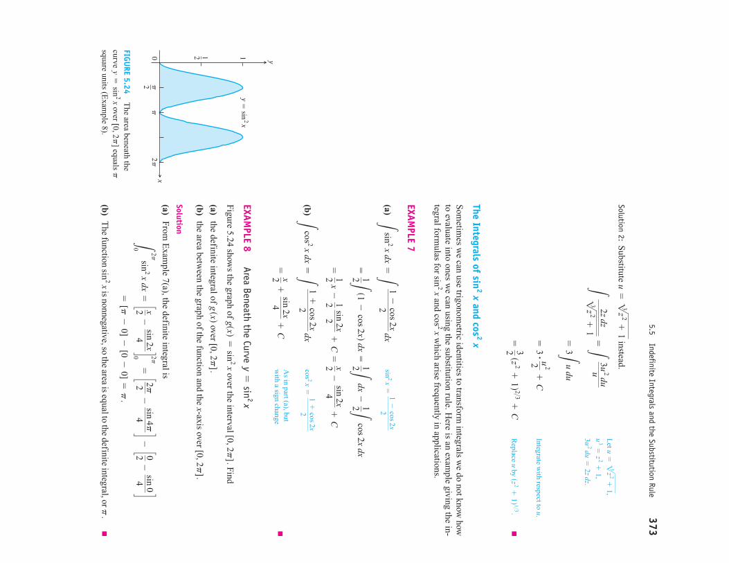
Solution 2:S
ubstitute instead.
Integrate with respect to u.
Replace u
by
The Integrals of and
Som
etimes w
e can use trigonometric identities to transform
integrals we do not know
howto evaluate into ones w
e can using the substitution rule. Here is an exam
ple giving the in-tegral form
ulas for and
which arise frequently in applications.
EXAMPLE 7
(a)
(b)
EXAMPLE 8
Area Beneath the Curve
Figure5.24
shows the graph of
over the interval Find
(a)the definite integral of
over
(b)the area betw
een the graph of the function and the x-axis over
Solution
(a)From
Exam
ple 7(a), the definite integral is
(b)T
hefunction
isnonnegative,so
thearea
isequalto
thedefinite
integral,orp
.sin
2 x
=[p
-0]
-[0
-0]
=p
.
L2p
0sin
2 x dx=c x2
-sin
2x4 d0 2
p
=c 2p2
-sin
4p
4 d-c 02
-sin
04 d
[0, 2p
].
[0, 2p
].gsxd
[0, 2p
].gsxd
=sin
2 x y=
sin2 x
=x2
+sin
2x4
+C
Lcos
2 x dx=L
1+
cos 2x2
dx
=12
x-
12 sin
2x2
+C
=x2
-sin
2x4
+C
=12L
s1-
cos 2xd dx=
12L dx
-12L
cos 2x dx
Lsin
2 x dx=L
1-
cos 2x2
dx
cos2 x
sin2 x
cos 2 xsin
2 x
sz2+
1d 1>3. =
32 sz
2+
1d 2>3+
C
=3 # u
22+
C
=3L
u du
L
2z dz
23
z2+
1=L
3u2 duu
u=2
3z
2+
1
5.5Indefinite Integrals and the Substitution Rule
373
Let
3u2 du
=2z dz.
u3=
z2+
1,
u=2
3z
2+
1,
sin2 x
=1
-cos 2x2
cos2 x
=1
+cos 2x2
As in part (a), but
with a sign change
02
��
�2
1
x
y
y � sin
2 x
12
FIGURE 5.24
The area beneath the
curve over
equals square units (E
xample 8).
p[0, 2p
]y
=sin
2 x
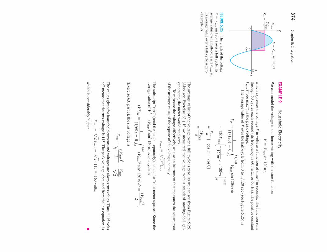
EXAMPLE 9
Household Electricity
We can m
odel the voltage in our home w
iring with the sine function
which expresses the voltage V
in volts as a function of time tin seconds. T
he function runsthrough 60 cycles each second (its frequency is 60 hertz, or 60 H
z). The positive constant
(“vee max”) is the peak voltage.
The average value of V
over the half-cycle from 0 to
sec (see Figure5.25) is
The average value of the voltage over a full cycle is zero, as w
e can see from Figure 5.25.
(Also see E
xercise 63.) If we m
easured the voltage with a standard m
oving-coil gal-vanom
eter, the meter w
ould read zero.To m
easure the voltage effectively, we use an instrum
ent that measures the square root
of the average value of the square of the voltage, namely
The subscript “rm
s” (read the letters separately) stands for “root mean square.” S
ince theaverage value of
over a cycle is
(Exercise 63, part c), the rm
s voltage is
The
valuesgiven
forhouseholdcurrents
andvoltages
arealw
aysrm
svalues.T
hus,“115 voltsac” m
eans that the rms voltage is 115. T
he peak voltage, obtained from the last equation, is
which is considerably higher.
Vm
ax=2
2 Vrm
s=2
2 #115L
163 volts,
Vrm
s=B
sVm
ax d 2
2=
Vm
ax
22
.
sV2dav
=1
s1>60d-
0 L
1>600
sVm
ax d 2 sin2 120
pt dt
=sV
max d 2
2,
V2=sV
max d 2 sin
2 120p
t
Vrm
s=2
sV2dav
.
=2V
maxp
.
=V
maxp
[-cos p
+cos 0]
=120V
max c-
1120p
cos 120p
td0 1>120 V
av=
1s1>120d
-0
L1>120
0 V
max sin
120p
t dt
1>120V
max
V=
Vm
ax sin 120p
t,
374Chapter 5: Integration
t
V0
V �
Vm
ax sin 120�
tV
max
Vav �
2Vm
ax�
1120
160
FIGURE 5.25
The graph of the voltage
over a full cycle. Itsaverage value over a half-cycle is Its average value over a full cycle is zero(E
xample 9).
2Vm
ax >p.
V=
Vm
ax sin 120p
t

374 Chapter 5: Integration
EXERCISES 5.5
Evaluating IntegralsEvaluate the indefinite integrals in Exercises 1–12 by using the givensubstitutions to reduce the integrals to standard form.
1. 2. Lx sin s2x2d dx, u = 2x2
L sin 3x dx, u = 3x
3.
4. L a1 - cos t2b2
sin t2
dt, u = 1 - cos t2
L sec 2t tan 2t dt, u = 2t
5.6.7.8.9.
10.
11.
a.U
sing b.
Using
12.
a.U
sing b.
Using
Evaluate the integrals in E
xercises 13–48.
13.14.
15.16.
17.18.
19.20.
21.22.
23.24.
25.26.
27.28.
29.30.
31.32.
33.
34.
35.36.L
6
cos ts2
+sin
td 3 dtL
sin s2t
+1d
cos2 s2t
+1d dt
Lcsc a
y-p
2 b cot a
y-p
2 b dy
L sec a
y+p2 b
tan ay
+p2 b
dy L
x1>3 sin
sx4>3
-8d dx
Lx
1>2 sin sx
3>2+
1d dx
Lr
4 a7-
r5
10 b3 dr
Lr
2 ar
3
18-
1b5 dr
Ltan
7 x2 sec
2 x2 dx
Lsin
5 x3 cos x3
dx
Ltan
2 x sec2 x dx
Lsec
2 s3x+
2d dx
Lsin
s8z-
5d dzL
cos s3z+
4d dz
L s1
+1xd 3
1x
dxL
1
1x s1
+1xd 2 dx
L
4y dy
22y
2+
1L
3y27
-3y
2 dy
L8u2
3u
2-
1 du
Lu2
41
-u
2 du
L
3 dx
s2-
xd 2L
1
25s
+4
ds
Ls2x
+1d 3 dx
L 23
-2s ds
u=2
5x+
8u
=5x
+8
L
dx
25x
+8
u=
csc 2u
u=
cot 2u
Lcsc
2 2u cot 2
u du
L 1x
2 cos2 a 1x b
dx, u
=-
1x
L 1x sin
2 sx3>2
-1d dx,
u=
x3>2
-1
L12sy
4+
4y2+
1d 2sy3+
2yd dy, u
=y
4+
4y2+
1
L
9r2 dr
21
-r
3 , u
=1
-r
3
Lx
3sx4-
1d 2 dx, u
=x
4-
1
L28s7x
-2d -
5 dx, u
=7x
-2
37.38.
39.40.
41.42.
43.
44.
45.46.
47.48.
Simplifying Integrals Step by Step
If you do not know w
hat substitution to make, try reducing the integral
step by step, using a trial substitution to simplify the integral a bit and
then another to simplify it som
e more. Y
ou will see w
hat we m
ean ifyou try the sequences of substitutions in E
xercises 49 and 50.
49.
a.follow
ed by then by
b.follow
ed by
c.
50.
a.follow
ed by then by
b.follow
ed by
c.
Evaluate the integrals in E
xercises 51 and 52.
51.
52.
Initial Value Problems
Solve the initial value problem
s in Exercises 53–58.
53.
54.
55.
56.drdu
=3
cos2 ap4
-ub
, rs0d
=p8
dsdt=
8 sin
2 at+p12 b
, ss0d
=8
dydx=
4x sx2+
8d -1>3,
ys0d=
0
dsdt=
12t s3t 2-
1d 3, ss1d
=3
L
sin 2u
2u
cos3 1u
du
L s2r
-1d cos 2
3s2r-
1d 2+
6
23s2r
-1d 2
+6
dr
u=
1+
sin2 sx
-1d
y=
1+
u2
u=
sin sx
-1d,
w=
1+y
2y
=sin
u,
u=
x-
1,
L 21
+sin
2 sx-
1d sin sx
-1d cos sx
-1d dx
u=
2+
tan3 x
y=
2+
uu
=tan
3 x,
w=
2+y
y=
u3,
u=
tan x
,L
18 tan
2 x sec2 x
s2+
tan3 xd 2
dx
L3x
52x
3+
1 dxL
x32
x2+
1 dx
L Ax
-1
x5
dxL
t 3s1+
t 4d 3 dt
Lsu
4-
2u
2+
8u
-2dsu
3-u
+2d du
Lss
3+
2s2-
5s+
5ds3s2+
4s-
5d ds
L
cos 2u
2u
sin2 2u
du
L 1u
2 sin 1u
cos 1u du
L
11t coss1
t+
3d dtL
1t 2 cos a 1t-
1b dt
L sec z tan
z
2sec z
dzL 2
cot y csc2 y dy
5.5Indefinite Integrals and the Substitution Rule
375
57.
58.
59.T
he velocity of a particle moving back and forth on a line is
for all t. If w
hen find
the value of sw
hen
60.T
he acceleration of a particle moving back and forth on a line is
for all
t. If
and w
hen find s
when
Theory and Examples
61.It looks as if w
e can integrate 2 sin xcos x
with respect to x
inthree different w
ays:
a.b.c.
=-
cos 2x2
+C
3 . 2 sin
x cos x=
sin 2x
L2
sin x cos x dx
=L sin
2x dx
=-
u2+
C2=
-cos
2 x+
C2
u=
cos x,
L2
sin x cos x dx
=L-
2u du
=u
2+
C1=
sin2 x
+C
1
u=
sin x
, L
2 sin
x cos x dx=L
2u du
t=
1 sec
.t=
0,
8 m/sec
y =s
=0
a=
d2s>dt 2
=p
2 cos pt m>sec
2
t=p>2
sec.
t=
0,
s=
0y
=ds>dt
=6
sin 2t m>sec
d2y
dx2
=4 sec
2 2x tan 2x,
y¿s0d=
4, ys0d
=-
1
d2s
dt 2=
-4
sin a2t
-p2 b
, s¿s0d
=100,
ss0d=
0C
an all three integrations be correct? Give reasons for your an-
swer.
62.T
he substitution gives
The substitution
gives
Can both integrations be correct? G
ive reasons for your answer.
63.(C
ontinuation of Exam
ple 9.)
a.S
how by evaluating the integral in the expression
that the average value of over a full cycle
is zero.
b.T
he circuit that runs your electric stove is rated 240 volts rms.
What is the peak value of the allow
able voltage?
c.S
how that
L1>60
0sV
max d 2 sin
2 120 p
t dt=sV
max d 2
120.
V=
Vm
ax sin 120
pt
1s1>60d
-0
L1>60
0V
max sin
120 p
t dt
Lsec
2 x tan x dx
=Lu du
=u
22+
C=
sec2 x
2+
C.
u=
sec x
Lsec
2 x tan x dx
=Lu du
=u
22+
C=
tan2 x
2+
C.
u=
tan x
376Chapter 5: Integration

376 Chapter 5: Integration
Substitution and Area Between Curves
There are two methods for evaluating a definite integral by substitution. The first methodis to find an antiderivative using substitution, and then to evaluate the definite integral byapplying the Fundamental Theorem. We used this method in Examples 8 and 9 of the pre-ceding section. The second method extends the process of substitution directly to definiteintegrals. We apply the new formula introduced here to the problem of computing the areabetween two curves.
Substitution Formula
In the following formula, the limits of integration change when the variable of integrationis changed by substitution.
5.6
THEOREM 6 Substitution in Definite IntegralsIf is continuous on the interval [a, b] and ƒ is continuous on the range of g, then
Lb
aƒsg sxdd # g¿sxd dx = L
gsbd
gsadƒsud du
g¿

ProofL
et Fdenote any antiderivative of ƒ. T
hen,
To use the formula, m
ake the same u-substitution
and you
would use to evaluate the corresponding indefinite integral. T
hen integrate the trans-form
ed integral with respect to u
from the value g
(a) (the value of uat
) to the valueg
(b) (the value of uat
).
EXAMPLE 1
Substitution by Two M
ethods
Evaluate
SolutionW
e have two choices.
Method 1:
Transform
the integral and evaluate the transformed integral w
ith the trans-form
ed limits given in T
heorem 6.
Evaluate the new
definite integral.
Method 2:
Transform
the integral as an indefinite integral, integrate, change back to x, anduse the original x-lim
its.
=23
c23>2
-0
3>2d=
23 c22
2d=
422
3
=23
css1d 3+
1d 3>2-ss-
1d 3+
1d 3>2d L
1
-1 3x
22x
3+
1 dx=
23 sx
3+
1d 3>2d-1
1
=23
sx3+
1d 3>2+
C
=23
u3>2
+C
L3x
22x
3+
1 dx=L 1
u du
=23
c23>2
-0
3>2d=
23 c22
2d=
422
3
=23
u3>2d0 2
=L2
0 1u du
L1
-1 3x
22x
3+
1 dx
L1
-1 3x
22x
3+
1 dx.
x=
bx
=a
du=
g¿sxd dxu
=gsxd
=Lgsbd
gsadƒsud du
.
=Fsuddu=
gsad
u=gsbd
=Fsgsbdd
-Fsgsadd
Lb
aƒsgsxdd #g¿sxd dx
=Fsgsxdddx=
a
x=b
5.6Substitution and Area Betw
een Curves377
= ƒsgsxddg¿sxd
= F¿sgsxddg¿sxd
ddx Fsgsxdd
Fundam
entalT
heorem, Part 2
Let
When
When x
=1, u
=s1d 3
+1
=2
.x
=-
1, u=s-
1d 3+
1=
0.
u=
x3+
1, du=
3x2 dx
.
Let u
=x
3+
1, du=
3x2 dx
.
Integrate with respect to u.
Replace u
by x3+
1.
Use the integral just found,
with lim
its of integration for x.
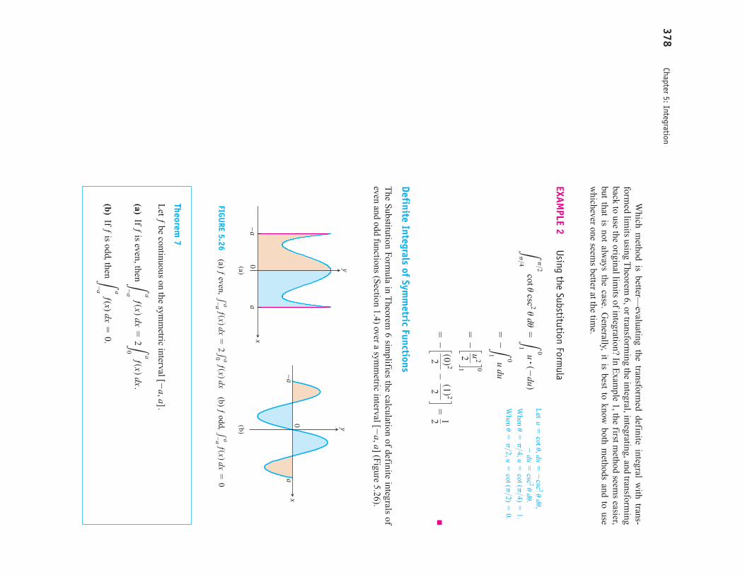
Which m
ethod is better—evaluating the transform
ed definite integral with trans-
formed lim
its using Theorem
6, or transforming the integral, integrating, and transform
ingback to use the original lim
its of integration? In Exam
ple 1, the first method seem
s easier,but that is not alw
ays the case. Generally, it is best to know
both methods and to use
whichever one seem
s better at the time.
EXAMPLE 2
Using the Substitution Formula
Definite Integrals of Symm
etric Functions
The S
ubstitution Formula in T
heorem 6 sim
plifies the calculation of definite integrals ofeven and odd functions (S
ection 1.4) over a symm
etric interval (Figure
5.26).[-
a, a]
=-c s0d 22
-s1d 2
2 d=
12
=-c u
22 d1 0
=-L
0
1u du
Lp>2p>4
cot u csc
2 u du
=L0
1u #s-
dud
378Chapter 5: Integration
x
y0a
–a
(b)
x
y0a
–a(a)
FIGURE 5.26
(a) ƒeven,
(b) ƒodd, 1
a-a ƒsxd dx
=0
1a-a ƒsxd dx
=21
a0 ƒsxd dx
Theorem 7
Let ƒ
be continuous on the symm
etric interval
(a)If ƒ
is even, then
(b)If ƒ
is odd, then La
-a ƒ(x) dx
=0.
La
-a ƒsxd dx
=2L
a
0ƒsxd dx.
[-a, a]. L
et
When
When u
=p>2, u
=cot (p>2)
=0.
u=p>4, u
=cot (p>4)
=1.
- du
=csc
2 u du.
u=
cot u, du=
-csc
2 u du,

Proof of Part (a)
The proof of part (b) is entirely sim
ilar and you are asked to give it in Exercise 86.
The assertions of
Theorem
7 remain true w
hen ƒis an integrable function (rather than
having the stronger property of being continuous), but the proof is somew
hat more diffi-
cult and best left to a more advanced course.
EXAMPLE 3
Integral of an Even Function
Evaluate
SolutionS
ince satisfies
it is even on the symm
et-ric interval
so
Areas Between Curves
Suppose w
e want to find the area of a region that is bounded above by the curve
below by the curve
and on the left and right by the lines and
(Figure5.27). T
he region might accidentally have a shape w
hose area we could find w
ithgeom
etry, but if ƒand g
are arbitrary continuous functions, we usually have to find the
area with an integral.
To see what the integral should be, w
e first approximate the region w
ith nvertical rec-
tangles based on a partition of [a,
b] (Figure5.28). T
he area of thekth rectangle (Figure
5.29) is
¢A
k=
height*
width
=[ƒsc
k d-
gsck d] ¢
xk .
P=5
x0 , x
1 ,Á, x
n 6
x=
bx
=a
y=
gsxd,y
=ƒsxd,
=2
a 325-
323+
12b=
23215
.
=2
c x55
-43
x3+
6xd0 2
L2
-2 sx
4-
4x2+
6d dx=
2L2
0sx
4-
4x2+
6d dx
[-2, 2],
ƒs-xd
=ƒsxd,
ƒsxd=
x4-
4x2+
6
L2
-2 sx
4-
4x2+
6d dx.
=2L
a
0ƒsxd dx
=La
0ƒsud du
+La
0ƒsxd dx
=La
0ƒs-
ud du+L
a
0ƒsxd dx
=-L
a
0ƒs-
uds-dud
+La
0ƒsxd dx
=-L
-a
0ƒsxd dx
+La
0ƒsxd dx
La
-a ƒsxd dx
=L0
-a ƒsxd dx
+La
0ƒsxd dx
5.6Substitution and Area Betw
een Curves379
Additivity R
ule forD
efinite Integrals
Order of Integration R
ule
Let
When
When x
=-
a, u=
a.
x=
0, u=
0.
u=
-x, du
=-
dx.
ƒis even, so
ƒs-ud
=ƒsud.
x
y
a
b
Low
er curvey �
g(x)
Upper curvey �
f(x)
FIGURE 5.27
The region betw
eenthe curves
and and the lines
and x=
b.
x=
ay
=gsxd
y=
ƒsxd
x
y
y � f(x)
y � g(x) b �
xn
xn�
1a
� x
0x
1
x2
FIGURE 5.28
We approxim
ate theregion w
ith rectangles perpendicularto the x-axis.
x
y
a
b
(ck , f(ck ))
f(ck ) � g(ck )
�A
kck
(ck , g(ck ))�
xk
FIGURE 5.29
The area
of the kthrectangle is the product of its height,
and its width, ¢
xk .
ƒsck d
-gsc
k d,
¢A
k

380Chapter 5: Integration
We then approxim
ate the area of the region by adding the areas of the nrectangles:
Riem
ann Sum
As
the sums on the right approach the lim
it because ƒ
andg
are continuous. We take the area of the region to be the value of this integral. T
hat is,
A=
limƒƒ P
ƒƒ :0 a n
k=1 [ƒsc
k d-
gsck d] ¢
xk=L
b
a[ƒsxd
-gsxd] dx.
1ba [ƒsxd
-gsxd] dx
7P 7:0
,
ALa n
k=1 ¢
Ak=a n
k=1 [ƒsc
k d-
gsck d] ¢
xk .
DEFINITION
Area Between Curves
If ƒand g
are continuous with
throughout [a,b], then the area ofthe region betw
een the curvesand
froma
tob
is the inte-gral of
from a
to b:A=L
b
a[ƒsxd
-gsxd] dx.
(f-
g)y
=gsxd
y=
fsxdƒsxd
Úgsxd
When applying this definition it is helpful to graph the curves. T
he graph reveals which
curve is the upper curve ƒand w
hich is the lower curve g. It also helps you find the lim
itsof integration if they are not already know
n. You m
ay need to find where the curves inter-
sect to determine the lim
its of integration, and this may involve solving the equation
for values of x. Then you can integrate the function
for the area be-tw
een the intersections.
EXAMPLE 4
Area Between Intersecting Curves
Find the area of the region enclosed by the parabola and the line
SolutionFirstw
e sketch the two curves (Figure
5.30). The lim
its of integration are foundby solving
and sim
ultaneously for x.
Equate ƒ(x) and g(x).
Rew
rite.
Factor.
Solve.
The region runs from
to
The lim
its of integration are T
he area between the curves is
=a4+
42-
83 b-a-
2+
12+
13 b=
92
=L2
-1 s2
+x
-x
2d dx=c2x
+x
22-
x33 d-
1
2
A=L
b
a[ƒsxd
-gsxd] dx
=L2
-1 [s2
-x
2d-s-
xd] dx
a=
-1, b
=2
.x
=2
.x
=-
1
x=
-1,
x=
2.
sx+
1dsx-
2d=
0
x2-
x-
2=
0
2-
x2=
-x
y=
-x
y=
2-
x2
y=
-x.
y=
2-
x2
ƒ-
gƒsxd
=gsxd
x
y0–1
12
(–1, 1)
(x, f(x))
y � 2 �
x2
(x, g(x))
�xy �
–x(2, –2)
FIGURE 5.30
The region in
Exam
ple 4 with a typical
approximating rectangle.

If the formula for a bounding curve changes at one or m
ore points, we subdivide the re-
gion into subregions that correspond to the formula changes and apply the form
ula for thearea betw
een curves to each subregion.
EXAMPLE 5
Changing the Integral to Match a Boundary Change
Find the area of the region in the first quadrant that is bounded above by and be-
low by the x-axis and the line
SolutionT
he sketch (Figure5.31) show
s that the region’s upper boundary is the graph ofT
he lower boundary changes from
for
to for
(there is agreement at
). We subdivide the region at
into subre-gions A
and B, show
n in Figure 5.31.T
he limits of integration for region A
are and
The left-hand lim
it for re-gion B
is To find the right-hand lim
it, we solve the equations
andsim
ultaneously for x:
Equate ƒ(x) and g(x).
Square both sides.
Rew
rite.
Factor.
Solve.
Only the value
satisfies the equation T
he value is an extrane-
ous root introduced by squaring. The right-hand lim
it is
We add the area of subregions A
and Bto find the total area:
Integration with Respect to y
If a region’s bounding curves are described by functions of y, the approximating rectangles
are horizontal instead of vertical and the basic formula has y
in place of x.
=23
s8d-
2=
103.
=23
s2d 3>2-
0+a 23
s4d 3>2-
8+
8b-a 23
s2d 3>2-
2+
4b =c 23
x3>2d0 2
+c 23 x
3>2-
x22
+2xd2 4
Total area
=
L2
0 1x dx
(')'*
area of A
+ L
4
2s1
x-
x+
2d dx('''')''''*
area of B
For 2
…x
…4:
ƒsxd-
gsxd=1
x-sx
-2d
=1x
-x
+2
For 0
…x
…2:
ƒsxd-
gsxd=1
x-
0=1
x
b=
4.
x=
11
x=
x-
2.
x=
4
x=
1, x
=4
.
sx-
1dsx-
4d=
0
x2-
5x+
4=
0
x=sx
-2d 2
=x
2-
4x+
4
1x
=x
-2
y=
x-
2y
=1x
a=
2.
b=
2.
a=
0
x=
2x
=2
2…
x…
4gsxd
=x
-2
0…
x…
2gsxd
=0
ƒsxd=1
x .
y=
x-
2.
y=1
x
5.6Substitution and Area Betw
een Curves381
HIS
TO
RIC
AL
BIO
GR
AP
HY
Richard D
edekind(1831–1916)
x
y0 1 2
42
y � �
x
y � 0
y � x
� 2
(x, f(x))
(x, f(x))
(x, g(x))
(x, g(x))
A
B(4, 2)
Area �
2
0 �x dx
Area �
4
2 (�x �
x � 2) dx
LL
FIGURE 5.31
When the form
ula for abounding curve changes, the area integralchanges to becom
e the sum of integrals to
match, one integral for each of the shaded
regions shown here for E
xample 5.

For regions like these
use the formula
In this equation ƒalw
ays denotes the right-hand curve and gthe left-hand curve, so
is nonnegative.
EXAMPLE 6
Find the area of the region in Exam
ple 5 by integrating with respect to y.
SolutionW
e first sketch the region and a typical horizontalrectangle based on a parti-
tion of an interval of y-values (Figure5.32). T
he region’s right-hand boundary is the lineso
The left-hand boundary is the curve
so T
he lower lim
it of integration is W
e find the upper limit by solving
andsim
ultaneously for y:
Rew
rite.
Factor.
Solve.
The upper lim
it of integration is (T
he value gives a point of intersection
belowthe x-axis.)
The area of the region is
This is the result of E
xample 5, found w
ith less work.
=4
+42
-83
=103
.
=c2y+
y22
-y
33 d0 2
=L2
0[2
+y
-y
2] dy
A=L
b
a[ƒsyd
-gsyd] dy
=L2
0[y
+2
-y
2] dy
y=
-1
b=
2.
y=
-1,
y=
2
sy+
1dsy-
2d=
0
y2-
y-
2=
0
y+
2=
y2
x=
y2
x=
y+
2y
=0
.gsyd
=y
2.x
=y
2,ƒsyd
=y
+2
.x
=y
+2
,
ƒsyd-
gsyd
A=L
d
c[ƒsyd
-gsyd] dy.
x�
f(y)
yy
x
x
x
y
x�
g(y)
0 c d
x�
g(y)
x�
f(y)
0 c d
0c dx
� f(y)
x�
g(y)
382Chapter 5: Integration
Equate
and gsyd=
y2.
ƒsyd=
y+
2
x
y
y � 0
24
0 1 2(g(y), y)
(f(y), y)f(y) �
g(y)
(4, 2)
x � y
� 2
x � y
2
�y
FIGURE 5.32
It takes two
integrations to find the area of thisregion if w
e integrate with respect to
x. It takes only one if we integrate
with respect to y
(Exam
ple 6).

Combining Integrals w
ith Formulas from
Geometry
The fastest w
ay to find an area may be to com
bine calculus and geometry.
EXAMPLE 7
The Area of the Region in Example 5 Found the Fastest W
ay
Find the area of the region in Exam
ple 5.
SolutionT
he area we w
ant is the area between the curve
and thex-axis, m
inusthe area of a triangle w
ith base 2 and height 2 (Figure5.33):
Conclusion from
Exam
ples 5–7
It is sometim
es easier to find the area between
two
curves by integrating with respect to y
instead of x. Also, it m
ay help to combine
geometry and calculus. A
fter sketching the region, take a mom
ent to think about the bestw
ay to proceed.
=23
s8d-
0-
2=
103 .
=23
x3>2d0 4
-2
Area
=L4
0 1x dx
-12
s2ds2d y=1
x, 0…
x…
4,
5.6Substitution and Area Betw
een Curves383
02
2
4
1 2
Area �
2
(4, 2)
x
y
y � 0
y � x
� 2
y � �
x
2
FIGURE 5.33
The area of the blue region
is the area under the parabola m
inus the area of the triangle (Exam
ple 7).y
=1x
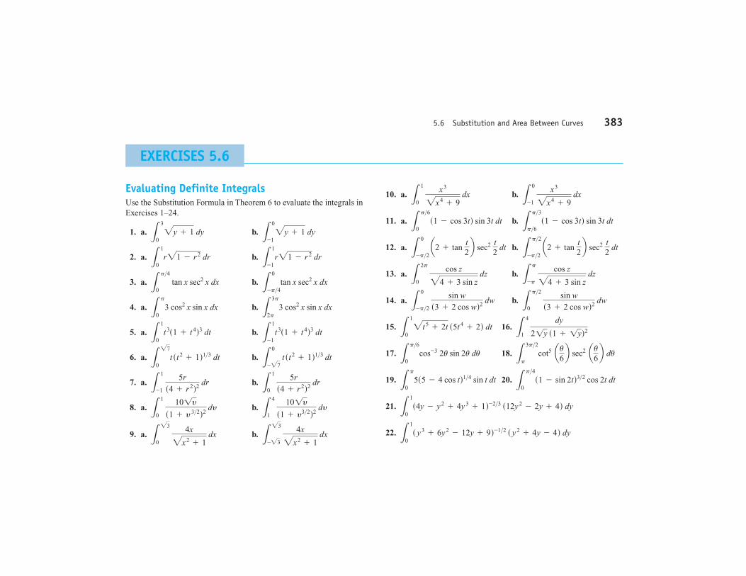
5.6 Substitution and Area Between Curves 383
EXERCISES 5.6
Evaluating Definite IntegralsUse the Substitution Formula in Theorem 6 to evaluate the integrals inExercises 1–24.
1. a. b.
2. a. b.
3. a. b.
4. a. b.
5. a. b.
6. a. b.
7. a. b.
8. a. b.
9. a. b. L23
-23
4x
2x2 + 1 dxL
23
0
4x
2x2 + 1 dx
L4
1
101ys1 + y3>2d2 dyL
1
0
101ys1 + y 3>2d2 dy
L1
0
5r
s4 + r2d2 drL
1
-1
5r
s4 + r2d2 dr
L0
-27 t st2 + 1d1>3 dtL
27
0t st2 + 1d1>3 dt
L1
-1t3s1 + t4d3 dtL
1
0t3s1 + t4d3 dt
L3p
2p3 cos2 x sin x dxL
p
03 cos2 x sin x dx
L0
-p>4tan x sec2 x dxLp>4
0 tan x sec2 x dx
L1
-1r21 - r2 drL
1
0r21 - r2 dr
L0
-12y + 1 dyL
3
02y + 1 dy
10. a. b.
11. a. b.
12. a. b.
13. a. b.
14. a. b.
15. 16.
17. 18.
19. 20.
21.
22. L1
0s y3 + 6y2 - 12y + 9d-1>2 s y2 + 4y - 4d dy
L1
0s4y - y2 + 4y3 + 1d-2>3 s12y2 - 2y + 4d dy
Lp>4
0s1 - sin 2td3>2 cos 2t dtL
p
05s5 - 4 cos td1>4 sin t dt
L3p>2p
cot5 au6b sec2 au
6b duL
p>60
cos-3 2u sin 2u du
L4
1
dy
21y s1 + 1yd2L1
02t5 + 2t s5t4 + 2d dt
Lp>2
0
sin w
s3 + 2 cos wd2 dwL
0
-p>2 sin w
s3 + 2 cos wd2 dw
Lp
-p
cos z
24 + 3 sin z dzL
2p
0
cos z
24 + 3 sin z dz
Lp>2
-p>2 a2 + tan t2b sec2
t2
dtL0
-p>2 a2 + tan t2b sec2
t2
dt
Lp>3p>6 s1 - cos 3td sin 3t dtL
p>60
s1 - cos 3td sin 3t dt
L0
-1
x3
2x4 + 9 dxL
1
0
x3
2x4 + 9 dx
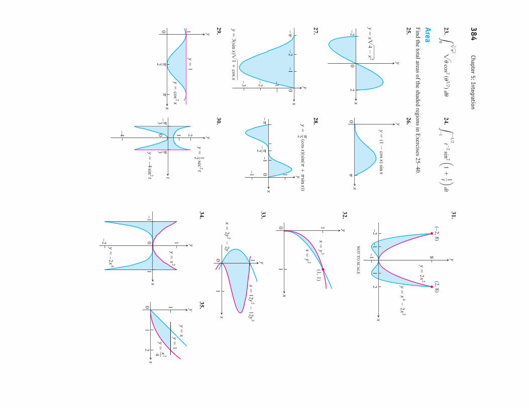
23.24.
AreaFind the total areas of the shaded regions in E
xercises 25–40.
25.26.
27.28.
29.30.
t
y
y �sec
2 t12
�3�3
–0 1 2
–4
y � –
4sin
2 t
x
y
��2
y � cos
2 x
0 1y �
1
x
y0–1
–�
–1 1
�2–
y �(cos x)(sin(�
� �
sin x))�2
x
y0–1
–1–2–3
–2–
�
y � 3(sin x)�
1 � cos x
x
y0�
y�
(1 � cos x) sin x
02
–2x
y
y � x�
4 � x
2
L-
1>2-
1t -
2 sin2 a1
+1t b
dtL2
3p
2
02u
cos2 su
3>2d du
31.
32.
33.
34.35.
x
y01
2
1
y � xy �
1
y �x
24x
y
–10–2 1
1
y � x
2
y � –2x
4
x
y0 1
1
x � 12y
2 � 12y
3
x � 2y
2 � 2y
01
1
x
y
(1, 1)
x � y
2
x � y
3
x
y
–2–1
12
–1 8(–2, 8)
(2, 8)
y � 2x
2
y � x
4 � 2x
2
NO
T T
O SC
AL
E
384Chapter 5: Integration

36.
37.38.
39.40.
Find the areas of the regions enclosed by the lines and curves in Exer-
cises 41–50.
41.
42.
43.
44.
45.
46.
47.
48.y
=x2
a2-
x2,
a7
0, and
y=
0
y=
x4-
4x2+
4 and
y=
x2
y=
7-
2x2
and y
=x
2+
4
y=
x2
and y
=-
x2+
4x
y=
x2-
2x and
y=
x
y=
x4
and y
=8x
y=
2x-
x2
and y
=-
3
y=
x2-
2 and
y=
2
x
y
–11
23
–2
2–5 4
(3, –5)
(–2, 4)y �
4 � x
2y � –x �
2
x
y5
–4
(–3, 5)
(1, –3)(–3, –3)
10
–3
y � x
2 � 4
y � –x
2 � 2x
01
2
1
x
y
y � x
2x
� y �
2
49.(H
ow m
any intersection pointsare there?)
50.
Find the areas of the regions enclosed by the lines and curves in Exer-
cises 51–58.
51.
52.
53.
54.
55.
56.
57.
58.
Find the areas of the regions enclosed by the curves in Exercises 59–62.
59.
60.
61.
62.
Find the areas of the regions enclosed by the lines and curves in Exer-
cises 63–70.
63.
64.
65.
66.
67.
68.
69.
70.
71.Find the area of the propeller-shaped region enclosed by the curve
and the line
72.Find the area of the propeller-shaped region enclosed by thecurves
and
73.Find the area of the region in the first quadrant bounded by theline
the line the curve
and the x-axis.
74.Find the area of the “triangular” region in the first quadrantbounded on the left by the y-axis and on the right by the curves
and
75.T
he region bounded below by the parabola
and above bythe line
is to be partitioned into two subsections of equal
area by cutting across it with the horizontal line
a.S
ketch the region and draw a line
across it that looksabout right. In term
s of c, what are the coordinates of the
points where the line and parabola intersect? A
dd them to
your figure.
y=
c
y=
c.
y=
4y
=x
2
y=
cos x.
y=
sin x
y=
1>x2,
x=
2,
y=
x,
x-
y1>5
=0
.x
-y
1>3=
0
x-
y=
0.
x-
y3=
0
y=
sec2 sp
x>3d and
y=
x1>3,
-1
…x
…1
x=
3 sin
y 2cos y
and x
=0,
0…
y…p>2
x=
tan2 y
and x
=-
tan2 y,
-p>4
…y
…p>4
y=
sec2 x,
y=
tan2 x,
x=
-p>4,
and x
=p>4
y=
sin sp
x>2d and
y=
x
y=
cos spx>2d
and y
=1
-x
2
y=
8 cos x
and y
=sec
2 x, -p>3
…x
…p>3
y=
2 sin
x and
y=
sin 2x,
0…
x…p
x+
y2=
3 and
4x+
y2=
0
x+
4y2=
4 and
x+
y4=
1, for
xÚ
0
x3-
y=
0 and
3x2-
y=
4
4x2+
y=
4 and
x4-
y=
1
x=
y3-
y2
and x
=2y
x=
y2-
1 and
x=
ƒ yƒ 21
-y
2
x-
y2>3
=0
and x
+y
4=
2
x+
y2=
0 and
x+
3y2=
2
x-
y2=
0 and
x+
2y2=
3
y2-
4x=
4 and
4x-
y=
16
x=
y2
and x
=y
+2
x=
2y2,
x=
0, and
y=
3
y=
ƒ x2-
4ƒ
and y
=sx
2>2d+
4
y=2
ƒ xƒ and
5y=
x+
6
5.6Substitution and Area Betw
een Curves385
x
y
–10 2
1–1
–22
(–2, –10) y � 2x
3 � x
2 � 5x
y � –x
2 � 3x
(2, 2)
x
y
30 6
–2
y �3 x
y ��
x3 x3
(3, 6)
(3, 1)
⎛⎝⎛⎝
–2, –3 2
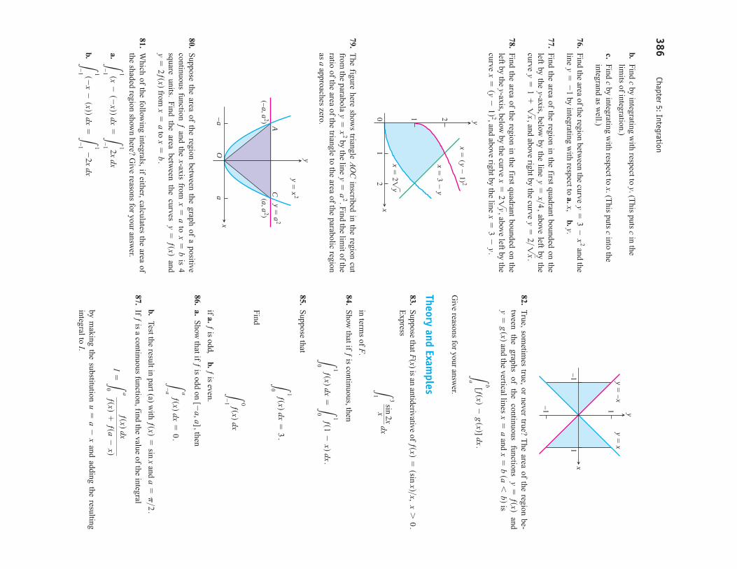
b.Find c
by integrating with respect to y. (T
his puts cin the
limits of integration.)
c.Find c
by integrating with respect to x. (T
his puts cinto the
integrand as well.)
76.Find the area of the region betw
een the curve and the
line by integrating w
ith respect to a.x,b.y.
77.Find the area of the region in the first quadrant bounded on theleft by the y-axis, below
by the line above left by the
curve and above right by the curve
78.Find the area of the region in the first quadrant bounded on theleft by the y-axis, below
by the curve above left by the
curve and above right by the line
79.T
he figure here shows triangle A
OC
inscribed in the region cutfrom
the parabola by the line
Find the limit of the
ratio of the area of the triangle to the area of the parabolic regionas a
approaches zero.
80.S
uppose the area of the region between the graph of a positive
continuous function ƒand the x-axis from
to
is 4square units. Find the area betw
een the curves and
from
to
81.W
hich of the following integrals, if either, calculates the area of
the shaded region shown here? G
ive reasons for your answer.
a.b.L1
-1 s-
x-sxdd dx
=L1
-1 -
2x dx
L1
-1 sx
-s-
xdd dx=L
1
-1 2x dx
x=
b.
x=
ay
=2ƒsxd
y=
ƒsxdx
=b
x=
a
x
y
CA
O–a
a
y�
x2
y�
a2
(a, a2)
(–a, a2)
y=
a2.
y=
x2
x
y0 1 2
12
x � 2�
y
x�
3�
y
x�
(y�
1) 2
x=
3-
y.
x=sy
-1d 2,
x=
21y
,
y=
2>1x
.y
=1
+1x
,y
=x>4
,
y=
-1
y=
3-
x2
82.T
rue, sometim
es true, or never true? The area of the region be-
tween
the graphs
of the
continuous functions
andand the vertical lines
and is
Give reasons for your answ
er.
Theory and Examples
83.S
uppose that F(x) is an antiderivative of
Express
in terms of F
.
84.S
how that if ƒ
is continuous, then
85.S
uppose that
Find
if a.ƒis odd,
b.ƒis even.
86.a.
Show
that if ƒis odd on
then
b.Test the result in part (a) w
ith and
87.If ƒ
is a continuous function, find the value of the integral
by making the substitution
and adding the resultingintegral to I.
u=
a-
x
I=L
a
0
ƒsxd dxƒsxd
+ƒsa
-xd
a=p>2
.ƒsxd
=sin
x
La
-a ƒsxd dx
=0
.
[-a, a],
L0
-1 ƒsxd dx
L1
0ƒsxd dx
=3
.
L1
0ƒsxd dx
=L1
0ƒs1
-xd dx
.
L3
1 sin
2xx
dx
ƒsxd=ssin
xd>x, x7
0.
Lb
a[ƒsxd
-gsxd] dx
.
x=
b sa6
bdx
=a
y=
gsxdy
=ƒsxd
x
y
–1
–1 1
1
y � –x
y � x
386Chapter 5: Integration
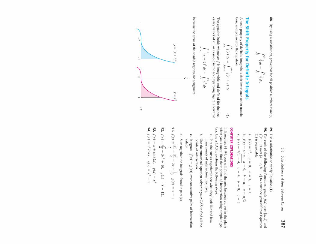
88.B
y using a substitution, prove that for all positive numbers x
and y,
The Shift Property for Definite IntegralsA
basic property of definite integrals is their invariance under transla-tion, as expressed by the equation.
(1)
The equation holds w
henever ƒis integrable and defined for the nec-
essary values of x. For example in the accom
panying figure, show that
because the areas of the shaded regions are congruent.
x
y01
–1–2
y�
(x�
2) 3y
� x
3
L-
1
-2sx
+2d 3 dx
=L1
0x
3 dx
Lb
aƒsxd dx
=Lb-
c
a-c
ƒsx+
cd dx.
Lxy
x 1t dt
=Ly
1 1t dt.
89.U
se a substitution to verify Equation (1).
90.For each of the follow
ing functions, graph ƒ(x) over [a,b] and
over to convince yourself that E
quation(1) is reasonable.
a.b.c.
COMPU
TER EXPLORATIONS
In Exercises 91–94, you w
ill find the area between curves in the plane
when you cannot find their points of intersection using sim
ple alge-bra. U
se a CA
S to perform
the following steps:
a.P
lot the curves together to see what they look like and how
many points of intersection they have.
b.U
se the numerical equation solver in your C
AS
to find all thepoints of intersection.
c.Integrate
over consecutive pairs of intersectionvalues.
d.S
um together the integrals found in part (c).
91.
92.
93.
94.ƒsxd
=x
2 cos x, gsxd
=x
3-
x
ƒsxd=
x+
sin s2xd,
gsxd=
x3
ƒsxd=
x42
-3x
3+
10, gsxd
=8
-12x
ƒsxd=
x33
-x
22-
2x+
13,
gsxd=
x-
1
ƒ ƒsxd-
gsxdƒ
ƒsxd=2
x-
4 , a
=4,
b=
8, c
=5
ƒsxd=
sin x,
a=
0, b
=p
, c
=p>2
ƒsxd=
x2,
a=
0, b
=1,
c=
1
[a-
c, b-
c]ƒsx
+cd
3875.6
Substitution and Area Between Curves

Chapter 5Questions to Guide Your Review
387
Chapter 5Questions to Guide Your Review
1.H
ow can you som
etimes estim
ate quantities like distance traveled,area, and average value w
ith finite sums? W
hy might you w
ant todo so?
2.W
hat is sigma notation? W
hat advantage does it offer? Give ex-
amples.
3.W
hat is a Riem
ann sum? W
hy might you w
ant to consider such asum
?
4.W
hat is the norm of a partition of a closed interval?
5.W
hat is the definite integral of a function ƒover a closed interval
[a,b]? When can you be sure it exists?
6.W
hat is the relation between definite integrals and area? D
escribesom
e other interpretations of definite integrals.
7.W
hat is the average value of an integrable function over a closedinterval? M
ust the function assume its average value? E
xplain.
8.D
escribe the rules for working w
ith definite integrals (Table 5.3).G
ive examples.
9.W
hat is the Fundam
ental Theorem
of Calculus? W
hy is it so im-
portant? Illustrate each part of the theorem w
ith an example.
10.H
ow does the F
undamental T
heorem provide a solution to the ini-
tial value problem
when ƒ
is continu-ous?
11.H
ow is integration by substitution related to the C
hain Rule?
12.H
ow can you som
etimes evaluate indefinite integrals by substitu-
tion? Give exam
ples.
13.H
ow does the m
ethod of substitution work for definite integrals?
Give exam
ples.
14.H
ow do you define and calculate the area of the region betw
eenthe graphs of tw
o continuous functions? Give an exam
ple.
dy>dx=
ƒsxd, ysx0 d
=y
0 ,
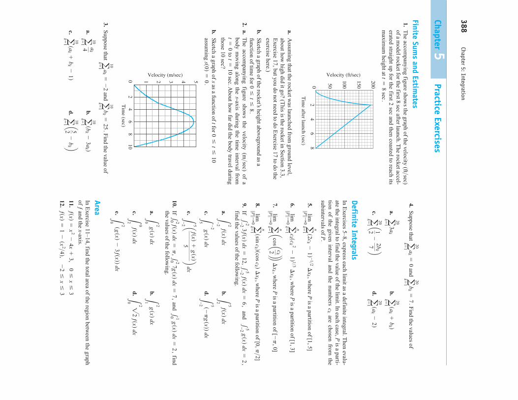
388Chapter 5: Integration
Chapter 5Practice Exercises
Finite Sums and Estim
ates1.
The accom
panying figure shows the graph of the velocity (ft
sec)of a m
odel rocket for the first 8 sec after launch. The rocket accel-
erated straight up for the first 2 sec and then coasted to reach itsm
aximum
height at
a.A
ssuming that the rocket w
as launched from ground level,
about how high did it go? (T
his is the rocket in Section 3.3,
Exercise 17, but you do not need to do E
xercise 17 to do theexercise here.)
b.S
ketch a graph of the rocket’s height aboveground as afunction of tim
e for 2.
a.T
he accompanying figure show
s the velocity (msec) of a
body moving along the s-axis during the tim
e interval fromto
About how
far did the body travel duringthose 10 sec?
b.S
ketch a graph of sas a function of tfor
assuming
3.S
uppose that and
Find the value of
a.b.
c.d.a 10
k=1 a 52
-b
k ba 10
k=1 sa
k+
bk-
1d
a 10
k=1 sb
k-
3ak d
a 10
k=1 a
k4
a 10
k=1 b
k=
25.
a 10
k=1 a
k=
-2
0 1
24
68
10
2 3 4 5
Tim
e (sec)
Velocity (m/sec)
ss0d=
0.
0…
t…
10
t=
10 sec.t=
0
>0
…t…
8.
24
68
0 50
100
150
200
Tim
e after launch (sec)
Velocity (ft/sec) t=
8 sec.
>4.
Suppose that
and Find the values of
a.b.
c.d.
Definite IntegralsIn E
xercises 5–8, express each limit as a definite integral. T
hen evalu-ate the integral to find the value of the lim
it. In each case, Pis a parti-
tion of the given interval and the numbers
are chosen from the
subintervals of P.
5.w
here Pis a partition of [1, 5]
6.w
here Pis a partition of [1, 3]
7.w
here Pis a partition of
8.w
here Pis a partition of
9.If
and find the values of the follow
ing.
a.b.
c.d.
e.
10.If
and find
the values of the following.
a.b.
c.d.
e.
AreaIn E
xercise 11–14, find the total area of the region between the graph
of ƒand the x-axis.
11.
12.ƒsxd
=1
-sx
2>4d, -
2…
x…
3
ƒsxd=
x2-
4x+
3, 0
…x
…3
L2
0sgsxd
-3ƒsxdd dx
L2
0 22
ƒsxd dxL
0
2ƒsxd dx
L2
1gsxd dx
L2
0gsxd dx
110 gsxd dx
=2
,1
20ƒsxd dx
=p
, 120 7gsxd dx
=7
,
L5
-2 a ƒsxd
+gsxd
5b
dx
L5
-2 s-p
gsxdd dxL
-2
5gsxd dx
L5
2ƒsxd dx
L2
-2 ƒsxd dx
15-2 gsxd dx
=2
,1
2-2 3ƒsxd dx
=12, 1
5-2 ƒsxd dx
=6
,
[0, p>2]lim
ƒƒ Pƒƒ :
0 a n
k=1 ssin
ck dscos c
k d ¢x
k ,
[-p
, 0]lim
ƒƒ Pƒƒ :
0 a n
k=1 acosa c
k2 bb ¢
xk ,
limƒƒ P
ƒƒ :0 a n
k=1 c
k sck
2-
1d 1>3 ¢x
k ,
limƒƒ P
ƒƒ :0 a n
k=1 s2c
k-
1d -1>2 ¢
xk ,
ck
a 20
k=1 sa
k-
2da 20
k=1 a 12
-2b
k
7 ba 20
k=1 sa
k+
bk d
a 20
k=1 3a
k
a 20
k=1 b
k=
7.
a 20
k=1 a
k=
0

13.
14.
Find the areas of the regions enclosed by the curves and lines in Exer-
cises 15–26.
15.
16.
17.
18.
19.20.
21.
22.
23.
24.
25.
26.
27.Find the area of the “triangular” region bounded on the left by
on the right by and above by
28.Find the area of the “triangular” region bounded on the left by
on the right by and below
by
29.Find the extrem
e values of and find the area of
the region enclosed by the graph of ƒand the x-axis.
30.Find the area of the region cut from
the first quadrant by the curve
31.Find the total area of the region enclosed by the curve and the lines
and
32.Find the total area of the region betw
een the curves and
for 0…
x…
3p>2
.y
=cos x
y=
sin x
y=
-1
.x
=y
x=
y2>3
x1>2
+y
1>2=
a1>2.
ƒsxd=
x3-
3x2
y=
1.
y=
6-
x,
y=1
x,
y=
2.
y=
x2,
x+
y=
2,
y=
8 cos x,
y=
sec2 x,
-p>3
…x
…p>3
y=
2 sin
x, y
=sin
2x, 0
…x
…p
y=
ƒ sin xƒ ,
y=
1, -p>2
…x
…p>2
y=
sin x,
y=
x, 0
…x
…p>4
y2=
4x+
4, y
=4x
-16
y2=
4x, y
=4x
-2
x=
4-
y2,
x=
0x
=2y
2, x
=0,
y=
3
x
y
01
1x
3�
�y
� 1, 0 �
x�
1
x3+1
y=
1, x
=0,
y=
0, for
0…
x…
1
x
y101
�x
� �
y�
1
1x
+1y
=1,
x=
0, y
=0
y=
x, y
=1>1
x, x
=2
y=
x, y
=1>x
2, x
=2
ƒsxd=
1-1
x , 0
…x
…4
ƒsxd=
5-
5x2>3,
-1
…x
…8
Initial Value Problems
33.S
how that
solves the initial value problem
34.S
how
that solves
the initial
valueproblem
Express the solutions of the initial value problem
s in Exercises 35 and
36 in terms of integrals.
35.
36.
Evaluating Indefinite IntegralsE
valuate the integrals in Exercises 37–44.
37.38.
39.
40.
41.42.
43.44.
Evaluating Definite IntegralsE
valuate the integrals in Exercises 45–70.
45.46.
47.48.
49.50.
51.52.
53.54.
55.56.L
p>40 cos
2 a4t-p4 b
dtLp
0 sin
2 5r dr
L1>20
x3s1
+9x
4d -3>2 dx
L1
1/8 x-
1>3s1-
x2>3d 3>2 dx
L1
0
dr
23
(7-
5r) 2L
1
0
36 dxs2x
+1d 3
L4
1 A 1
+1uB 1>2
1u
duL
4
1
dtt1
t
L27
1x-
4/3 dxL
2
1 4y
2 dy
L1
0s8s
3-
12s2+
5d dsL
1
-1 s3x
2-
4x+
7d dx
L sec u
tan u 2
1+
sec u du
L 1
t sin s2t 3>2d dt
L st
+1d 2
-1
t 4 dt
L at-
2t bat+
2t b dt
L a1
22u
-p
+2 sec
2 s2u
-pdb
du
Ls2u
+1
+2
cos s2u
+1dd d
u Lstan
xd -3>2 sec
2 x dxL
2scos xd -1>2 sin
x dx
dydx=2
2-
sin2 x ,
ys-1d
=2
dydx=
sin x
x,
ys5d=
-3
d2y
dx2
=2sec x tan
x;
y¿s0d=
3, ys0d
=0
.
y=1
x0 A 1+
22sec tB dt
d2 y
dx2
=2
-1x2 ;
y¿s1d=
3, ys1d
=1
.
y=
x2+L
x
1 1t dt
Chapter 5Practice Exercises
389
57.58.
59.60.
61.62.
63.64.
65.66.
67.68.
69.70.
Average Values71.
Find the average value of
a.over
b.over
72.Find the average value of
a.over [0, 3]
b.over [0, a]
73.L
et ƒbe a function that is differentiable on [a,b]. In C
hapter 2w
edefined the average rate of change of ƒ
over [a,b] to be
and the instantaneous rate of change of ƒat x
to be In this
chapter we defined the average value of a function. For the new
def-inition of average to be consistent w
ith the old one, we should have
Is this the case? Give reasons for your answ
er.
74.Is it true that the average value of an integrable function over aninterval of length 2 is half the function’s integral over the interval?G
ive reasons for your answer.
75.C
ompute the average value of the tem
perature function
for a 365-day year. This is one w
ay to estimate the annual m
eanair tem
perature in Fairbanks, Alaska. T
he National W
eather Ser-
vice’s official figure, a numerical average of the daily norm
alm
ean air temperatures for the year, is 25.7ºF, w
hich is slightlyhigher than the average value of ƒ(x). Figure 3.33
shows w
hy.
76.Specific heat of a gas
Specific heat
is the amount of heat re-
quired to raise the temperature of a given m
ass of gas with con-
Cy
ƒsxd=
37 sin
a2p
365 sx
-101db
+25
ƒsbd-
ƒsadb
-a
=average value of ƒ¿ on [a, b]. ƒ¿sxd.
ƒsbd-
ƒsadb
-a
y=2
ax
y=2
3x
[-k, k]
[-1, 1]
ƒsxd=
mx
+b
Lp
2>4p
2>36
cos1t
2t sin
1t dt
Lp>30
tan
u
22 sec u
du
Lp>40
sec
2 x
s1+
7 tan
xd 2>3 dxLp>20
3
sin x cos x
21
+3
sin2 x
dx
L2p>3
0 cos -
4 ax2 b
sin a
x2 b dx
Lp>2-p>2 15
sin4 3x cos 3x dx
L1
-1 2x sin
s1-
x2d dx
Lp>20
5ssin xd 3>2 cos x dx
L3p>4
p>4 csc z cot z dz
L0
-p>3 sec x tan
x dx
Lp
0 tan
2 u3 du
L3p
p
cot 2 x6 dx
L3p>4
p>4 csc
2 x dxLp>30
sec2 u du
stant volume by 1ºC
, measured in units of cal
deg-mole (calories
per degree gram m
olecule). The specific heat of oxygen depends
on its temperature T
and satisfies the formula
Find the average value of for
and the tem-
perature at which it is attained.
Differentiating IntegralsIn E
xercises 77–80, find .
77.78.
79.80.
Theory and Examples
81.Is it true that every function
that is differentiable on [a,b] is itself the derivative of som
e function on [a,b]? Give rea-
sons for your answer.
82.S
uppose that F(x) is an antiderivative of
Ex-
press in term
s of Fand give a reason for your
answer.
83.Find
if E
xplain the main steps in
your calculation.
84.Find
if E
xplain the main steps
in your calculation.
85.A
new parking lot
To meet the dem
and for parking, your town
has allocated the area shown here. A
s the town engineer, you have
been asked by the town council to find out if the lot can be built
for $10,000. The cost to clear the land w
ill be $0.10 a square foot,and the lot w
ill cost $2.00 a square foot to pave. Can the job be
done for $10,000? Use a low
er sum estim
ate to see. (Answ
ersm
ay vary slightly, depending on the estimate used.)
0 ft
36 ft
54 ft
51 ft
49.5 ft
54 ft
64.4 ft
67.5 ft
42 ft
Ignored
Vertical spacing �
15 ft
y=1
0 cos x s1>s1-
t 2dd dt.dy>dx
y=1
1x 2
1+
t 2 dt.dy>dx 1
10 2
1+
x4 dx
ƒsxd=2
1+
x4.
y=
ƒsxd
y=L
2
sec x 1
t 2+
1 dt
y=L
1
x
63
+t 4 dt
y=L
7x2
2 2
2+
cos3 t dt
y=L
x
2 22
+cos
3 t dt
dy>dx
20°…
T…
675°CCy
Cy
=8.27
+10
-5 s26T
-1.87T
2d.
>390
Chapter 5: Integration
T T
86.S
kydivers A and B
are in a helicopter hovering at 6400 ft. Sky-
diver A jum
ps and descends for 4 sec before opening her para-chute. T
he helicopter then climbs to 7000 ft and hovers there.
Forty-five seconds after A leaves the aircraft, B
jumps and de-
scends for 13 sec before opening his parachute. Both skydivers
descend at 16 ftsec w
ith parachutes open. Assum
e that the sky-divers fall freely (no effective air resistance) before their para-chutes open.
a.A
t what altitude does A
’s parachute open?
b.A
t what altitude does B
’s parachute open?
c.W
hich skydiver lands first?
Average Daily InventoryA
verage value is used in economics to study such things as average
daily inventory. If I(t) is the number of radios, tires, shoes, or w
hateverproduct a firm
has on hand on day t(we call I
an inventory function),
the average value of Iover a tim
e period [0, T] is called the firm
’s av-erage daily inventory for the period.
If his the dollar cost of holding one item
per day, the product is the average daily holding cost
for the period.avsId #h
Average daily inventory
=avsId
=1T
LT
0Istd dt.
>
87.A
s a wholesaler, T
racey Burr D
istributors receives a shipment of
1200 cases of chocolate bars every 30 days. TB
D sells the choco-
late to retailers at a steady rate, and tdays after a shipm
ent ar-rives,
its inventory
of cases
on hand
is W
hat is TB
D’s average daily inventory for the 30-
day period? What is its average daily holding cost if the cost of
holding one case is 3¢ a day?
88.R
ich Wholesale Foods, a m
anufacturer of cookies, stores its casesof cookies in an air-conditioned w
arehouse for shipment every 14
days. Rich tries to keep 600 cases on reserve to m
eet occasionalpeaks
in dem
and, so
a typical
14-day inventory
function is
The daily holding cost for each
case is 4¢ per day. Find Rich’s average daily inventory and aver-
age daily holding cost.
89.S
olon Container receives 450 drum
s of plastic pellets every 30days. T
he inventory function (drums on hand as a function of
days) is Find the average daily inventory. If
the holding cost for one drum is 2¢ per day, find the average daily
holding cost.
90.M
itchell Mailorder receives a shipm
ent of 600 cases of athleticsocks every 60 days. T
he number of cases on hand tdays after the
shipment
arrives is
Find the
averagedaily inventory. If the holding cost for one case is
¢ per day,find the average daily holding cost.
1>2Istd
=600
-202
15t.
Istd=
450-
t 2>2.
Istd=
600+
600t, 0…
t…
14.
0…
t…
30.
Istd=
1200-
40t,
391Chapter 5
Practice Exercises
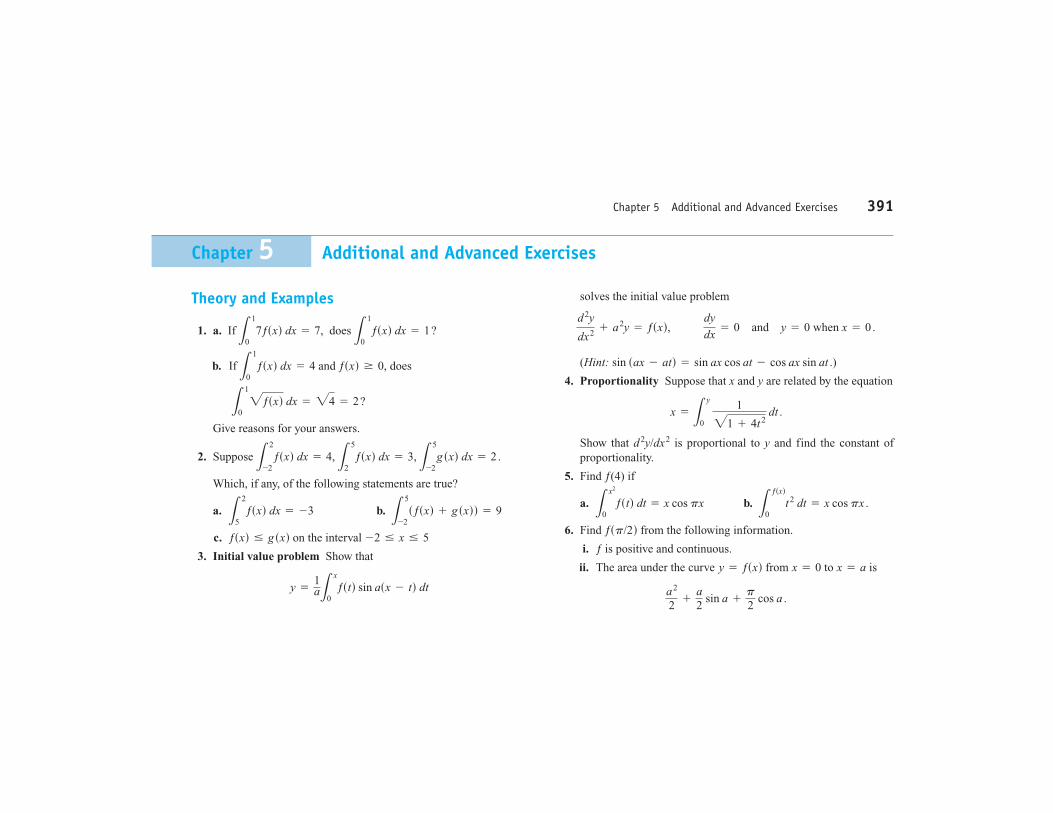
Chapter 5 Additional and Advanced Exercises 391
Chapter 5 Additional and Advanced Exercises
Theory and Examples
1. a. If
b. If
Give reasons for your answers.
2. Suppose
Which, if any, of the following statements are true?
a. b.
c. on the interval
3. Initial value problem Show that
y = 1aL
x
0ƒstd sin asx - td dt
-2 … x … 5ƒsxd … g sxdL
5
-2sƒsxd + g sxdd = 9L
2
5ƒsxd dx = -3
L2
-2ƒsxd dx = 4, L
5
2ƒsxd dx = 3, L
5
-2g sxd dx = 2.
L1
02ƒsxd dx = 24 = 2?
L1
0ƒsxd dx = 4 and ƒsxd Ú 0, does
L1
07ƒsxd dx = 7, does L
1
0ƒsxd dx = 1?
solves the initial value problem
(Hint: )
4. Proportionality Suppose that x and y are related by the equation
Show that is proportional to y and find the constant ofproportionality.
5. Find ƒ(4) if
a. b.
6. Find from the following information.
i. ƒ is positive and continuous.
ii. The area under the curve from to is
a2
2+ a
2 sin a + p
2 cos a .
x = ax = 0y = ƒsxd
ƒsp/2dL
ƒsxd
0t2 dt = x cos px .L
x2
0ƒstd dt = x cos px
d2y/dx2
x = Ly
0
1
21 + 4t2 dt .
sin sax - atd = sin ax cos at - cos ax sin at .
d2y
dx2 + a2y = ƒsxd, dy
dx= 0 and y = 0 when x = 0.
7.T
he area of the region in the xy-plane enclosed by the x-axis, thecurve
and the lines and
is
equal to for all
Find ƒ(x).
8.P
rove that
(Hint:
Express the integral on the right-hand side as the difference
of two integrals. T
hen show that both sides of the equation have
the same derivative w
ith respect to x.)
9.F
inding a curveFind the equation for the curve in the xy-plane
that passes through the point if its slope at x
is always
10.Shoveling dirt
You sling a shovelful of dirt up from
the bottomof a hole w
ith an initial velocity of 32 ft/sec. The dirt m
ust rise 17ft above the release point to clear the edge of the hole. Is thatenough speed to get the dirt out, or had you better duck?
Piecewise Continuous Functions
Although w
e are mainly interested in continuous functions, m
anyfunctions in applications are piecew
ise continuous. A function ƒ(x) is
piecewise continuous on a closed interval
Iif ƒ
has only finitelym
any discontinuities in I, the limits
exist and are finite at every interior point of I, and the appropriate one-sided lim
its exist and are finite at the endpoints of I. All piecew
isecontinuous functions are integrable. T
he points of discontinuity subdi-vide I
into open and half-open subintervals on which ƒ
is continuous,and the lim
it criteria above guarantee that ƒhas a continuous exten-
sion to the closure of each subinterval. To integrate a piecewise con-
tinuous function, we integrate the individual extensions and add the
results. The integral of
(Figure5.34) over
is
The F
undamental T
heorem applies to piecew
ise continuous func-tions w
ith the restriction that is expected to equal
ƒ(x) only at values of xat w
hich ƒis continuous. T
here is a similar re-
striction on Leibniz’s R
ule below.
Graph the functions in E
xercises 11–16 and integrate them over
their domains.
sd>dxd1xa ƒstd dt
=32
+83
-1
=196
.
=cx-
x22 d-
1
0
+c x33 d0 2
+c-xd2 3
L3
-1 ƒsxd dx
=L0
-1 s1
-xd dx
+L2
0x
2 dx+L
3
2s-
1d dx
[-1, 3]
ƒsxd=•
1-
x,-
1…
x6
0
x2,
0
…x
62
-1,
2
…x
…3
limx:
c- ƒsxd and
limx:
c+ ƒsxd
3x2+
2.
s1, -1d
Lx
0 aLu
0ƒstd dtb
du=L
x
0ƒsudsx
-ud du
.
b7
1.
2b
2+
1-2
2
x=
bx
=1
y=
ƒsxd, ƒsxdÚ
0,
11.
12.
13.
14.
15.
16.
17.Find the average value of the function graphed in the accom
pany-ing figure.
18.Find the average value of the function graphed in the accom
pany-ing figure.
x
y1
12
30
x
y01
2
1
hsrd=•
r,-
1…
r6
0
1-
r2,
0…
r6
1
1,1
…r
…2
ƒsxd=•
1,-
2…
x6
-1
1-
x2,
-1
…x
61
2,1
…x
…2
hszd=e 2
1-
z,0
…z
61
s7z-
6d -1>3,
1…
z…
2
gstd=e
t,0
…t6
1
sin p
t,1
…t…
2
ƒsxd=e 2
-x ,
-4
…x
60
x2-
4,0
…x
…3
ƒsxd=e
x2>3,
-8
…x
60
-4,
0…
x…
3
392Chapter 5: Integration
x
y2
20
31
–1
1 3 4–1
y � x
2
y � 1 �
x
y � –1
FIGURE 5.34
Piecew
ise continuous functionslike this are integrated piece by piece.

Leibniz’s RuleIn applications, w
e sometim
es encounter functions like
defined by integrals that have variable upper limits of integration and
variable lower lim
its of integration at the same tim
e. The first integral
can be evaluated directly, but the second cannot. We m
ay find the de-rivative of either integral, how
ever, by a formula called L
eibniz’s Rule.
ƒsxd=L
x2
sin x s1
+td dt
and gsxd
=L21
x
1x
sin t 2 dt,
at which the carpet is being unrolled. T
hat is, A(x) is being in-
creased at the rate
At the sam
e time, A
is being decreased at the rate
the width at the end that is being rolled up tim
es the rate . T
henet rate of change in A
is
which is precisely L
eibniz’s Rule.
To prove the rule, let Fbe an antiderivative of ƒ
on [a,b]. Then
Differentiating both sides of this equation w
ith respect to xgives the
equation we w
ant:
Chain R
ule
Use L
eibniz’s Rule to find the derivatives of the functions in E
x-ercises 19–21.
19.20.
21.
22.U
se Leibniz’s R
ule to find the value of xthat m
aximizes the value
of the integral
Problem
s like this arise in the mathem
atical theory of politicalelections. S
ee “The E
ntry Problem
in a Political Race,” by S
tevenJ. B
rams and P
hilip D. S
traffin, Jr., in Political Equilibrium
, PeterO
rdeshook and
Kenneth
Shepfle,
Editors,
Kluw
er-Nijhoff,
Boston, 1982, pp. 181–195.
Approximating Finite Sum
s with Integrals
In many applications of calculus, integrals are used to approxim
ate fi-nite sum
s—the reverse of the usual procedure of using finite sum
s toapproxim
ate integrals.
Lx+
3
x ts5
-td dt.
gsyd=L
21y
1y
sin t 2 dt
ƒsxd=L
sin x
cos x
11
-t 2 dt
ƒsxd=L
x
1/x 1t dt =ƒsysxdd d
ydx-
ƒsusxdd dudx.
=F¿sysxdd d
ydx-
F¿susxdd dudx
ddxLysxd
usxdƒstd dt
=ddx
cFsysxdd-
Fsusxddd
Lysxd
usxdƒstd dt
=Fsysxdd
-Fsusxdd.
dAdx=
ƒsysxdd dydx
-ƒsusxdd dudx
,
du>dxƒsusxdd dudx
,
ƒsysxdd dydx
.
dy>dx
Chapter 5Additional and Advanced Exercises
393
t
y
0
Uncovering
Covering
f(u(x))y�
f(t)f(y(x))
u(x)
y(x)A(x)
�f(t)dty(x)
u(x)L
FIGURE 5.35
Rolling and unrolling a carpet: a geom
etricinterpretation of L
eibniz’s Rule:
dAdx=
ƒsysxdd dydx
-ƒsusxdd dudx
.
Leibniz’s RuleIf ƒ
is continuous on [a, b] and if u(x) and y(x) are dif-ferentiable functions of x
whose values lie in [a,
b],then
.ddx
Lysxd
usxdƒstd dt
=ƒsysxdd d
ydx-
ƒsusxdd dudx
Figure5.35
gives a geometric interpretation of L
eibniz’s Rule. It
shows a carpet of variable w
idth ƒ(t) that is being rolled up at the leftat the sam
e time x
as it is being unrolled at the right. (In this interpre-tation, tim
e is x, not t.) At tim
e x, the floor is covered from u(x) to y(x).
The rate
at which the carpet is being rolled up need not be the
same as the rate
at which the carpet is being laid dow
n. At any
given time x, the area covered by carpet is
Asxd=L
ysxd
usxdƒstd dt.
dy>dx
du>dx
At w
hat rate is the covered area changing? At the instant x,A
(x) is in-creasing by the w
idth ƒ(y(x)) of the unrolling carpet times the rate

For example, let’s estim
ate the sum of the square roots of the first
npositive integers,
The integral
is the limit of the upper sum
s
Therefore, w
hen nis large,
will be close to
and we w
ill have
The follow
ing table shows how
good the approximation can be.
nR
oot sumR
elative error
1022.468
21.08250
239.04235.70
1.4%100
671.46666.67
0.7%1000
21,09721,082
0.07%
23.E
valuate
by showing that the lim
it is
and evaluating the integral.
24.S
ee Exercise 23. E
valuate
limn:
q 1n
4 s13+
23+
33+
Á+
n3d.
L1
0x
5 dx
limn:
q 1
5+
25+
35+
Á+
n5
n6
1.386>22.468L
6%
s2>3dn3>2
Root sum
=21
+22
+Á
+2n
=S
n #n3>2
L23
n3/2.
2>3S
n
x
y0
y � �
x
11
n2n
n � 1
n
= 21
+22
+Á
+2n
n3>2
.
Sn=A
1n # 1n
+A2n
# 1n+
Á+A
nn # 1n
L1
0 1x dx
=23
x3>2d0 1
=23
21
+22
+Á
+2n
.25.
Let ƒ(x) be a continuous function. E
xpress
as a definite integral.
26.U
se the result of Exercise 25 to evaluate
a.b.c.
What can be said about the follow
ing limits?
d.e.
27.a.
Show
that the area of an n-sided regular polygon in a circle
of radius ris
b.Find the lim
it of as
Is this answer consistent w
ithw
hat you know about the area of a circle?
28.A
differential equationS
how that
satisfies both of the following conditions:
i.ii.and
when
29.A
function defined by an integralT
he graph of a function ƒconsists of a sem
icircle and two line segm
ents as shown. L
et
a.Find g
(1).b.
Find g(3).
c.Find
d.Find all values of x
on the open interval at w
hich ghas a relative m
aximum
.
e.W
rite an equation for the line tangent to the graph of gat
f.Find the x-coordinate of each point of inflection of the graphof g
on the open interval
g.Find the range of g.
s-3, 4d.
x=
-1
.
s-3, 4d
gs-1d.
y
13
–3
y � f(x)
–1–1 1 3
x
gsxd=1
x1 ƒstd dt.
x=p
.y¿
=-
2y
=1
y–=
-sin
x+
2 sin
2x1px
cos 2t dt+
1y
=sin
x+
n:q
.A
n An=
nr2
2 sin
2pn
.
An
limn:
q
1n15 s1
15+
215
+3
15+
Á+
n15d
limn:
q
1n17 s1
15+
215
+3
15+
Á+
n15d
limn:
q 1n
asin pn
+sin
2pn
+sin
3pn
+Á
+sin
npn b
.
limn:
q
1n16 s1
15+
215
+3
15+
Á+
n15d,
limn:
q 1n
2 s2+
4+
6+
Á+
2nd,
limn:
q 1n
cƒ a 1n b
+ƒ
a 2n b+
Á+
ƒ a nn bd
394Chapter 5: Integration

Chapter 5Technology Application Projects
395
Chapter 5Technology Application Projects
Mathem
atica/Maple M
oduleU
sing R
ieman
n S
um
s to Estim
ate Areas,Volu
mes,an
d Len
gths of C
urves
Visualize and approxim
ate areas and volumes in Part I.
Mathem
atica/Maple M
oduleR
ieman
n S
um
s,Defin
ite Integrals,an
d the F
un
damen
tal Th
eorem of C
alculu
sParts I, II, and III develop R
iemann sum
s and definite integrals. Part IV continues the developm
ent of the Riem
ann sum and definite integral
using the Fundam
ental Theorem
to solve problems previously investigated.
Mathem
atica/Maple M
oduleR
ain C
atchers,E
levators,and R
ocketsPart I illustrates that the area under a curve is the sam
e as the area of an appropriate rectangle for examples taken from
the chapter. You w
illcom
pute the amount of w
ater accumulating in basins of different shapes as the basin is filled and drained.
Mathem
atica/Maple M
oduleM
otion A
long a S
traight L
ine,P
art IIY
ou will observe the shape of a graph through dram
atic animated visualizations of the derivative relations am
ong the position, velocity, andacceleration. Figures in the text can be anim
ated using this software.
Mathem
atica/Maple M
oduleB
endin
g of Beam
sS
tudy bent shapes of beams, determ
ine their maxim
um deflections, concavity and inflection points, and interpret the results in term
s of a beam’s
compression and tension.

![Math 103 –Rimmer 5.1 The Area Problem 5.3 The Definite ...11/13/2013 2 Math 103 –Rimmer 5.1 The Area Problem f x x( ) = 2 on the interval 1,5[ ] 5.3 The Definite Integral using](https://img.pdfslide.us/doc/110x75/60ccfec843b2d255d3257463/math-103-arimmer-51-the-area-problem-53-the-definite-11132013-2-math-103.jpg)
![The Definite Integral - Math - The University of Utah · 2013. 1. 4. · 25B Definite Integral 3 Definition of the Definite Integral Let f be a function that is defined on [a,b]](https://img.pdfslide.us/doc/110x75/60a2bfa42907903993233547/the-definite-integral-math-the-university-of-2013-1-4-25b-definite-integral.jpg)

![PROFESSIONAL MATHEMATICS - SBTE Home Page · Web view01.10 The Definite integral, Properties of the definite integral. Problem of area by Integration method. [05] 01.11 The Definite](https://img.pdfslide.us/doc/110x75/5ac648e17f8b9a12608e1259/professional-mathematics-sbte-home-view0110-the-definite-integral-properties.jpg)