© The Aerospace Corporation

517 COMPARISON OF ARTIFICIAL INTELLIGENCE AND STATISTICAL TECHNIQUES FOR

PROBABILISTIC FORECASTING OF SKY CONDITION

Timothy J. Hall, Carl N. Mutchler, Greg J. Bloy, Rachel N. Thessin, Stephanie K. Gaffney and J. J. Lareau The Aerospace Corporation

15049 Conference Center Drive Chantilly, VA 20151

1. INTRODUCTION A range of military, civil and commercial activities require cloud-free sky conditions. Passive optical or thermal remote sensors, such as those on unmanned aerial systems, need a cloud-free-line-of-sight in order to sense their targets (Norquist 1999). Solar energy available to fuel photovoltaic power generation is strongly modulated by clouds (Girodo et al. 2006) due to their ability to reflect incoming shortwave radiation, combined with their high spatial and temporal variability. Additionally, electricity demand on power grids is correlated to the amount of solar irradiance. Very short-range (i.e., up to 6-hr) sky condition forecasts are useful to decision makers for these applications. In this paper, we present findings from the development and testing of six, advanced obs-based prediction algorithms. These algorithms have emerged from a number of technical disciplines including statistics, applied mathematics, artificial intelligence (AI), cognitive psychology, engineering, and knowledge discovery in databases. The time frame from near-zero up to approximately six hours into the future represents a sweet spot for obs-based weather forecasting techniques (Bankert and Hadjimichael 2007, Hansen 2007, Vislocky and Fritsch 1997). Each algorithm chosen for this investigation was implemented to produce 1, 2, 3, 4 and 5-hr probabilistic forecasts of cloud-free (i.e., clear) sky condition for six areas of regard (AORs) representing different weather regimes within the continental United States (CONUS) (Fig. 1). The AORs are labeled according to familiar map features associated with the location of the area’s center pixel including Boston, Buffalo, Cape Canaveral (Cape), Denver, Ft Hood, and Corresponding author address: Tim Hall, The Aerospace Corporation, 8455 Colesville Rd. Silver Spring, MD 20910; email: Timothy.J.Hall@aero.org

St Louis. Performance potential was assessed through receiver operating characteristic (ROC) analysis. Other performance metrics included accuracy, sharpness, expected best cost (EBC), and reliability. All forecast algorithms, along with three additional standard baseline methods included for comparison purposes, were applied to two types of forecast “targets” within each AOR: (1) A local target comprised of the 4 x 4-km pixel demarcated by the points at the center of each square in Fig. 1; and (2) A regional target comprised of a 100 x 100-km area centered on each local target. The forecast objective for the local target was to determine the probability of clear for a “point” (i.e., a single pixel). For the regional target, the objective was to forecast the probability of ≥ 75% clear over the 10,000 km2 area. The 75% threshold was an arbitrary choice. The regional target type was included to compare the ability to forecast for a specific point to forecasting the sky condition across an area. The advanced, obs-based algorithms tested in this investigation outperformed the three baseline forecast techniques in nearly every regard at all forecast intervals in the six AORs. The findings presented in this paper represent a significant extension of research previously reported in Hall et al. (2009), and validates the concept presented in Hall et al. (2010a). 2. DATA The research database for this project, which spans from 1 May 2003 to 29 June 2008, consists of features extracted from meteorological satellite (METSAT) imagery, and meteorological parameters derived or extracted from analysis fields generated by the NCEP’s Eta model data assimilation system (EDAS) (Black 1994). The Eta analyses used in this investigation were extracted from a North American sector archived at 3-hr temporal

Figure 1: Map showing six CONUS areas of regard for this investigation. The point at the center of each area is the local target pixel. The inner square represents the regional (100 x 100-km area) target. The outer square (demarcated by the dashed line) depicts the 1000 x 1000-km extent of the satellite data used to build the feature database for the AOR. The outer squares for Buffalo and Boston extend into southern Canada. (Reprinted courtesy of NASA) resolution, 40-km horizontal spatial resolution, and 25 vertical levels. These data are maintained for research in the NCAR Computational & Information Systems Laboratory (CISL) Research Data Archive (RDA) (http://dss.ucar.edu). Cloud structural features were extracted (following cloud detection) from half-hourly digital METSAT imagery collected by NOAA Geostationary Operational Environmental Satellites (GOES-10 and GOES-12) downloaded from the National Climate Data Center (NCDC). Once the GOES data were processed, a cloud detection algorithm was applied based on the bispectral composite threshold (BCT) technique (Jedlovec et al. 2008). An attractive feature of the BCT method is that it provides relatively consistent cloud detection day and night. The result of applying the BCT algorithm was a five-year, half-hourly time series of cloud-no cloud (CNC) image composites, each representing a map of the clouds at a specific observation time. A 5-yr database comprised of 105 features was built for each of the six AORs. The features were a mix of real and categorical variables extracted or derived from the EDAS model analyses, satellite-based CNC composites and astronomical calculations (e.g., solar zenith angle). The meteorological parameters extracted from the EDAS analyses included variables such as potential temperature (θ), pressure, wind and geopotential height, and parameters derived

from them such as the mean layer vector wind (MLVW) (Blanchard and Lopez 1985) and dry static stability (Δθ/Δz). Given the three-hour time-step between each successive EDAS analysis, these data were interpolated temporally to populate the feature databases at the half-hourly frequency of the CNC composites. Since one of our objectives was to develop an approach that could be applied globally, EDAS moisture-related variables were excluded from use due to the unreliable quality of moisture parameters in these type of analyses (especially in data-sparse regions). Fifty cloud structural features were extracted from the CNC maps and IR imagery. The cloud features fall into five categories:

(1) Static sky condition features that represent the percent coverage of cloudy or clear pixels at the current observation time in some region near or around the target

(2) Static sky condition features stratified by MLVW

(3) Dynamic sky condition features created by analyzing the change (or trend) in percent area coverage of cloudy or clear conditions over an interval of time (e.g., 6 hr).

(4) Features that capture the persistency of a particular sky condition over an interval of time.

(5) IR image statistical features derived from the distribution of brightness temperatures in each 10.7-µm image including mean, variance, skew, and kurtosis.

A complete list of the features can be found in Hall et al. (2010a). For algorithm development, feature selection, and testing, the feature database was divided into two subsets. The first three years were designated as training data. The last two years of data were reserved for testing. All performance metrics, discussed below, are based on validation against the 2-yr test dataset. Witten and Frank (2005) summarize a number of strategies used to prune feature sets prior to application of a prediction algorithm. One of the most effective ways to select features is manually, based on domain subject matter expertise. Other strategies include: data-mining using machine learning algorithms or linear regression; and elimination of highly correlated features. All of these methods were applied against the training data in this investigation to assist with feature selection.

Data-mining was applied based on decision trees as implemented in the MATLAB Statistics

Toolbox and in the commercial See5 software package based on Quinlan (1986). Random Forest variable importance lists (Breiman 2001) and single feature k-nn trials provided additional insights. Linearly correlated features were identified using multiple linear regression and principal component analyses. The insights gained from these feature selection techniques were used to develop feature lists for the advanced, obs-based methods described in section 4. Several of the algorithms used all or nearly all of the features in the master set. 3. BASELINE FORECAST METHODS Three forecast methods were applied to establish performance baselines. at all forecast intervals in the six AORs. a. Basic Persistence (BP) BP (i.e., the future weather condition will be the same as the current weather condition) is the simplest form of obs-based forecasting. BP of clear for any given forecast interval was taken to be a 0% or 100% probability of clear at forecast time based on the initial sky condition. For the local target, this translates to a 100% forecast probability of clear if the initial sky condition was clear in the CNC composite. For the regional target, the BP forecast was translated to a 100% probability of ≥ 75% clear in the future given an initial condition of ≥ 75% clear. b. Conditional-Expectancy-of-Persistence (CEP) CEP, a term coined by Enger et al. (1962), was developed as an objective tool for operational forecasters to help them predict future conditions by matching an initial condition (e.g., the current state of the atmosphere) with historical conditions by categorizing the initial condition in terms of stratified climatological data. CEP is also referred to as the persistence climatology, conditional climatology, persistence probability, or conditional persistence. CEP-based cloud forecasting techniques using space-based observations have been applied by Kelly (1988), Combs et al. (2004), Connell et al. (2001), Hall et al. (1998), and Reinke et al. (2003). In this paper, CEP is similarly based on METSAT data. For this investigation, CEP was derived using the 3-yr training dataset and calculated as the probability of clear at each forecast interval (1, 2, 3, 4, and 5 hr) given the current (or initial) sky

condition (i.e., cloudy or clear), based on training data events within ± 1 hr and ± 30 d of that time of day and day of year. There was no differentiation between true persistence and recurrence in these calculations. c. Satellite Cloud Climatology (SCC) SCC forecasts were based on the prior probability of cloud-free conditions at each local or regional target calculated using the 3-yr training dataset for given (time of day, day of year) combinations. For all observations within ± 1 hr and ± 30 d, the percentage of occurrences with clear conditions were used as the climatological sky condition probability of clear for that time of day and day of year. 4. ADVANCED, OBS-BASED FORECAST METHODS Six prediction methods were implemented in this study including two statistical techniques, three predictive learning algorithms, and one ensemble technique based on the forecasts of the two top-performers (out of the other five). a. k-nn Analog Forecast (KAF) Algorithm Analog forecasting involves predicting future weather conditions based on the outcome of similar past events or patterns. k-nn is a statistical technique for nonparametric density estimation (Fukunaga 1990) that was adopted as a classification method in the 1960s (Johns 1961). k-nn algorithms classify based on identification of the closest points in multi-dimensional feature space. These nearest neighbor vectors in feature space comprise the analogs.

As described by Hall et al. (2010b), one version of a k-nn algorithm was applied to both target types in all six AORs. Implementation required a number of decisions including feature selection, feature similarity assessment, feature weighting, overall feature vector similarity scoring, and choice of k (i.e., the number of neighbors or analogs). k =100 was used for all AORs and forecast intervals for both target types. For each test case, 100 analogs were identified in the training data. The percentage of cases among these analogs that turned out clear was interpreted as the forecasted probability of clear for the test case.

The particular feature subset used to identify the analog ensembles for a forecast was tailored to both target types in each AOR at the 1, 2, 3,

4, and 5-hr forecast intervals. Each feature set was comprised of no more than 16 features to mitigate the known susceptibility of k-nn algorithms to the “curse of dimensionality” (Bellman 1961, Beyer et al. 1999). b. Single Feature Bayes Classifier (SFB) If the statistical distribution of a pattern is known, the Bayes decision rule gives the minimum-error-rate classification (Duda and Hart 2000). The Bayes classifier is an ideal classifier that always predicts the class which is most likely to occur with a given set of inputs. However, it is rare to have the information necessary to determine the Bayes classifier (Sutton 2005). Given discreetized feature X which can be used for prediction, Bayes’ theorem yields the probability that the future condition will be clear:

P(Clear | X) = P(X)

P(Clear) Clear)|P(X

With about 50,000 training cases in this investigation, the data distribution of each sky condition (i.e., cloudy or clear), along with the associated prior probabilities is regarded as well known for each feature. Given this, the best performing feature for each target type, AOR, and forecast interval was used as a single feature Bayes classifier (SFB) to generate probabilistic forecasts based on Bayes’ theorem. The probabilities on the right-hand side of the equation above were computed using the training data to produce forecasts for each case in the test data. The same approach could be applied to combinations of two or more features. However, estimation of the joint distribution of two or more features would require a minimum of about 100,000 training cases. c. Regression Tree (RT) RT is a non-parametric, recursive partitioning technique that can result in relatively simple functions of predictors that are easy to interpret and use. RT was based on Breiman et al. (1998) as implemented in the MATLAB Statistics Toolbox. The underlying strategy is non-incremental learning from examples (Quinlan 1986). A tree is constructed by repeatedly splitting data, defined by a simple rule based on a single, explanatory feature. At each split, the data is partitioned into two mutually exclusive groups that are as homogeneous as possible. Splitting

proceeds until an overlarge tree is grown, which is then pruned. Breiman’s method is a “greedy”, top-down approach that is characterized by an overfit of the model to the data. A unique tree was formed for both target types in each AOR for all five forecast intervals based on the training data. Initially, a very large tree was created for each model with thousands of leaf nodes. This tree was then pruned through a two-step process. First, the overfit tree was trimmed using a MATLAB pruning algorithm which evaluated the error at each leaf-node pair with a common parent. This algorithm eliminated the leaves (thereby making the parent a leaf) when removal reduced the overall classification error. Trimming proceeded to a user-defined level corresponding to a tree size of ~100 nodes. Second, the tree size with the minimum error was determined using N-fold cross-validation with N = 10. Trees pruned to ≤ 10 nodes typically exhibited the best performance based on developmental trials using the Buffalo feature set. The top node in every tree was always one of the METSAT-derived cloud structural variables. The pruned decision trees were used to generate forecasts by applying them to the test data feature vectors. The probability of clear was a direct output from the tree in each case. d. Random Forest (RF)

RF was developed by Leo Breiman (Breiman 2001) to improve the performance of decision tree algorithms such as RT. RF creates an ensemble of decision trees by training on a random redistribution of the training set. Each distribution is generated by randomly drawing M samples (with replacement), where M is the size of the training set. A tree is grown on a fixed-size subset of features randomly drawn on each round. The algorithm outputs the class that is the mode of the output by the individual trees.

For each AOR, target type, and forecast interval, an ensemble of 100 trees was grown by the RF algorithm based on the 3-yr training dataset. Each tree in the ensemble was then applied to the feature vectors in the test data, resulting in a classification of cloudy or clear. The number of trees that “voted” for clear was interpreted as the forecast probability of clear for each test case.

RF was designed to effectively utilize large feature sets. However, RF can be susceptible to noise from extraneous or redundant features. One result of the feature selection process described earlier was a pruned feature set of 78

of the original 105 features in which some redundant and highly correlated features had been eliminated. Use of this pruned feature set for RF resulted in a small, positive (but statistically significant) performance improvement during training trials on the Buffalo AOR database. RF was implemented using software developed by Breiman available at the following internet site: (http://www.stat.berkeley.edu/~breiman/RandomForests). e. Neural Network (NN) The first application of a NN to forecasting involved weather prediction (Hu 1964). NNs are attractive for weather forecasting because of their ability to generalize to new instances after learning the data presented to them even if the feature data contain noisy information. Zhang et al. (1998) provide a good overview of forecasting with NNs. Our NN topology consisted of 105 nodes in the input layer, one logistic hidden node with full connections to the input, and one logistic output node that was also fully connected to the input layer nodes. In this architecture, the hidden layer modeled the non-linearities of the system while the direct input-to-output connections modeled the near-linear relations. NN models were implemented in MATLAB with the NETLAB toolbox (Nabney 2001) using the scaled conjugate gradients method for training. For both target types, a separate network was trained for each of the five forecast intervals in each of the six AORs. Each network was trained with 75% of the features in the training database, substituting for missing features in a FIFO manner. Data were normalized by subtracting the mean and dividing by the standard deviation for each feature. The remaining 25% of the training data were used for validation during training of each model. After each training epoch, the model predictions were checked against the validation data and an error score computed. In order to mitigate over-fitting of the models, the model parameters (i.e., weights) corresponding to the epoch that produced the most accurate validation dataset score were output. Root mean square error was used as the error metric. The number of epochs was limited to a maximum of 100.

Figure 2: Neural network topology. f. Multi-Algorithm Ensemble (ME) Three approaches to utilizing the predictions from the eight other forecast methods together as a multi-algorithm ensemble were tested including Bayesian probability (Fukunaga 1990), Beta Transformed Linear Opinion Pool (Gneiting and Ranjan 2008), and simple linear combination of probabilities. Performance results from developmental testing on the Buffalo AOR feature set showed that the simple average (i.e., an equally weighted linear combination) of the top two performing prediction algorithms (RF and NN) provided the best ensemble results. Based on these findings, the linear combination of RF and NN was implemented as the ME algorithm across all AORs for both target types. 5. RESULTS No single measure of performance can completely and unambiguously describe the quality of a forecast system. Therefore, our approach to assess each forecast method was multifaceted. Overall performance potential was assessed using relative operating characteristic (ROC) analysis. Additional insights were gleaned from an ensemble of metrics, including sharpness, accuracy, a value metric we refer to as expected best cost (EBC), and reliability. The following conventions are used throughout this paper to describe sky condition events: E = 0 corresponds to clear conditions for

the local target and ≥ 75% clear total areal coverage for the regional target. Likewise, E = 1 corresponds to cloudy conditions for the local target and < 75% clear for the regional target. a. ROC analysis ROC analysis is useful to assess the overall performance potential of a probabilistic weather forecast technique since the process of forecasting a discrete meteorological event is analogous to the detection of a signal against a background of noise (Harvey et al. 1992, Mason and Graham 2002). Following Mason (1982), algorithm performance in a series of instances can be represented using a 2 x 2 verification matrix (Fig. 3). Figure 3: Forecast verification matrix. From these data, two additional parameters can be derived called the hit rate and false alarm rate. The hit rate (i.e., hits divided by total positives) represents the probability of the event forecasted to occur (E), given the event occurred. The false alarm rate (i.e., false alarms divided by total negatives) is the probability of forecasting E, given it did not occur. Given a set of probabilistic forecasts, categorical forecasts can be created by using a probabilistic threshold (e.g., 0.5). To produce the data for a ROC curve, a set of hit rate/false alarm rate pairs is generated by varying the decision threshold from 0 to 1 in small increments. These data are then plotted on a two-dimensional graph with hit rate on the y-axis and false alarm rate on the x-axis. The ROC curves for each algorithm for the Boston local and regional target types are shown in Figs. 4 and 5, respectively. These data are generally representative of the results for the other targets. Perfect forecast performance potential is represented on a ROC graph by the upper left-hand corner. A ROC curve lying along the major diagonal line from (0,0) to (1,1) represents random forecasting, in which a forecast of Y (i.e., event will occur) is no more likely to precede an occurrence of the event than

it is to precede a non-occurrence. In Figs. 4 and 5, one can easily determine through visual inspection that the performance potential of each of the advanced, obs-based algorithms (i.e., KAF, SFB, RT, RF, NN, and ME) exceeds CEP and BP at the 1-, 3-, and 5-hr forecast intervals. The same holds for the 2- and 4-hr intervals (not shown). When any classifier that produces only a class decision is applied to a single set of test events, it yields a single verification matrix which, in turn, corresponds to one point in ROC space. In Figs 4 and 5, the points indicated by the triangles in each graph correspond to BP ROC points for each forecast interval. Fig. 6 contains the 1- and 5-hr ROC curves for Buffalo, Cape, and St Louis local target type forecasts for all six advanced algorithms. The spread in performance potential represented by the width of the region created by each set of ROC curves is slightly greater at 5 hr than 1 hr. The spread between the curves is attributable to a combination of performance variation between algorithms and between AORs. The spread at 1 hr mostly reflects inter-AOR variation. The area under the ROC curve, called the ROC score, provides a “single-number-summary” of forecast algorithm performance potential (Harvey et al. 1992, Mason and Graham 2002). When the forecast system has some skill the ROC score will exceed 0.5. The ROC scores for each forecast algorithm at each forecast interval (averaged over all six AORs) are recorded in Table 1. ME had the highest ROC score for all 30 local target cases (not shown), and 28 of 30 regional target cases. RF had the highest ROC score for the Ft Hood AOR, regional target type for 4- and 5-hr forecasts. Note that the average ROC scores for the advanced, obs-based algorithms always exceeded CEP and SCC. Except for SCC, the ROC scores (and hence the performance potential) decrease with increasing forecast interval. b. Sharpness Sharpness indicates the tendency of a probabilistic forecast method to correctly assign extreme probability values (i.e., the tendency toward correct categorical forecasts). Forecast performance (in terms of sharpness) is dependent on the amount of separation between the probability values output by an algorithm when the true class is clear and when the true class is cloudy. Therefore, a histogram of the probabilities for those cases that turned out

observed noobserved yes

correct negativesmisses

false alarmshits

Fore

cast

Total NegativesTotal PositivesTotal

Correct NegativesMisses

False AlarmsHits

Occurred (Y)

Observation

Did Not Occur (N)

Will Occur (Y)

Will Not Occur (N)

observed noobserved yes

correct negativesmisses

false alarmshits

Fore

cast

Total NegativesTotal PositivesTotal

Correct NegativesMisses

False AlarmsHits

Occurred (Y)

Observation

Did Not Occur (N)

Will Occur (Y)

Will Not Occur (N)

Figure 4: Forecasting clear ROC curves for the Boston AOR, local target type. Each graph contains the 1, 2, 3, 4 and 5-hr ROC curves for the advanced algorithm identified above the plot (solid), the 1, 3, and 5-hr ROC curves for CEP (dashed), and ROC points (triangles) for all five forecast intervals.

Figure 5: Forecasting clear ROC curves for the Boston AOR, regional target type. Each graph contains the 1, 2, 3, 4 and 5-hr ROC curves for the advanced algorithm identified above the plot (solid), the 1, 3, and 5-hr ROC curves for CEP (dashed), and ROC points (triangles) for all five forecast intervals.

Figure 6: Forecasting clear ROC curves for all six advanced, obs-based algorithms from the Buffalo, Cape, and St Louis AORs for 1-hr (blue) and 5-hr (red) forecast intervals. Random forecasting is indicated by the dashed line between (0,0) and (1,1). clear, and one for those cases that turned out cloudy were used to graphically assess sharpness. Sharper examples are ones where most of the density mass given a cloudy outcome is near zero, and most of the density mass given a clear outcome is near one.

In Fig. 7, sharpness can be qualitatively assessed for 1, 3 and 5-hr Boston, regional target type forecasts for CEP, KAF, SFB, RT, RF, NN, and ME. For the purposes of comparing algorithm performance, these data are generally representative of the results across all of the targets for both the local and regional types. The NN forecasts were the top performer in terms of sharpness across the AORs. c. Accuracy Accuracy for this investigation was taken as the percent correct match (PCM) defined as the percent of total forecasts (i.e., total forecasts = hits + correct negatives + misses + false alarms) that turned out to be correct (i.e., either a hit or a correct negative). It is derived from the parameters in the verification matrix (Fig. 3) as (hits + correct negatives)/(total forecasts). Determination of PCM requires choosing a probabilistic decision threshold at which the forecast is made. Given a forecast sky condition probability provided by any given forecast algorithm, a threshold of 0.5 was used to

Table 1: Upper chart contains ROC scores for the local target type for each algorithm at every forecast interval, averaged over all six AORs. Lower chart similarly contains ROC scores for the regional target type.

ROC Scores, Local Target Type 1 Hr 2 Hr 3 Hr 4 Hr 5 Hr ME 0.947 0.917 0.892 0.870 0.851 RF 0.944 0.912 0.887 0.866 0.847 NN 0.946 0.914 0.887 0.864 0.842 KAF 0.940 0.901 0.873 0.851 0.834 RT 0.939 0.903 0.873 0.847 0.825 SFB 0.937 0.891 0.863 0.835 0.809 CEP 0.872 0.832 0.801 0.778 0.758 SCC 0.610 0.609 0.609 0.609 0.609 ROC Scores, Regional Target Type 1 Hr 2 Hr 3 Hr 4 Hr 5 Hr ME 0.973 0.944 0.920 0.898 0.878 RF 0.970 0.940 0.916 0.894 0.875 NN 0.971 0.942 0.915 0.891 0.869 KAF 0.969 0.935 0.910 0.883 0.862 RT 0.964 0.929 0.897 0.871 0.847 SFB 0.966 0.922 0.892 0.864 0.837 CEP 0.919 0.869 0.835 0.808 0.785 SCC 0.617 0.616 0.615 0.615 0.615 transform each probabilistic forecast into a categorical forecast of cloudy or clear. This threshold minimizes the probability of error, P(error) which is equal to 1 – P(correct forecast). PCM is the maximum likelihood estimator for P(correct forecast). In terms of accuracy, the ME algorithm dominated as the top performing algorithm by small, but not always statistically significant margins for both the local and regional target types. It was the top algorithm for 26 out of 30 local target cases, and 22 out of 30 regional target cases. RF was the top performer in terms of accuracy for the remaining 12 of out of 60 cases. Fig. 8 highlights the performance of the five, advanced obs-based algorithms (aside from ME) including KAF, SFB, RT, RF, and NN for both the regional and local target types. The bar graphs display the percentage of all occurrences (out of 30) that each algorithm was 1st, 2nd, 3rd... with regard to accuracy for each individual case. ME was omitted from these graphs in order to focus on the accuracy performance of the five prediction algorithms that utilized the feature databases. It is clear in the figure that the NN

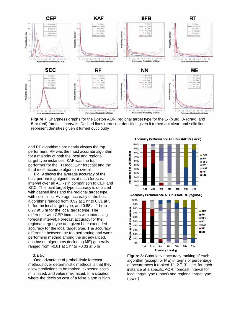
and RF algorithms are nearly always the top performers. RF was the most accurate algorithm for a majority of both the local and regional target type instances. KAF was the top performer for the Ft Hood, 1-hr forecast and the third most accurate algorithm overall. Fig. 9 shows the average accuracy of the best performing algorithms at each forecast interval over all AORs in comparison to CEP and SCC. The local target type accuracy is depicted with dashed lines and the regional target type with solid lines. Average accuracy of the best algorithms ranged from 0.92 at 1 hr to 0.81 at 5 hr for the local target type, and 0.88 at 1 hr to 0.77 at 5 hr for the local target type. The difference with CEP increases with increasing forecast interval. Forecast accuracy for the regional target type at a given hour exceeded accuracy for the local target type. The accuracy difference between the top performing and worst performing method among the six advanced, obs-based algorithms (including ME) generally ranged from ~0.01 at 1 hr to ~0.03 at 5 hr. d. EBC One advantage of probabilistic forecast methods over deterministic methods is that they allow predictions to be ranked, expected costs minimized, and value maximized. In a situation where the decision cost of a false alarm is high

Figure 8: Cumulative accuracy ranking of each algorithm (except for ME) in terms of percentage of occurrences it ranked 1st, 2nd, 3rd, etc. for each instance at a specific AOR, forecast interval for local target type (upper) and regional target type (lower)

Figure 7: Sharpness graphs for the Boston AOR, regional target type for the 1- (blue), 3- (gray), and 5-hr (red) forecast intervals. Dashed lines represent densities given it turned out clear, and solid lines represent densities given it turned out cloudy

Figure 9: Accuracy of top performing algorithm averaged across all AORs at each forecast interval. The top performing algorithm with regard to accuracy was ME in a majority of cases. Average BP accuracy (not shown) was very close to CEP at all forecast intervals. (in terms of resources or risk), actions that cause expenditure of resources or unpalatable exposure to risk should be taken only when there is high confidence in the event occurring. Conversely, if the cost of a miss, rather than of a false alarm, is prohibitively high, the number of actions should be increased by relaxing the required confidence level (i.e., probability threshold) that prompts a decision to act. So, each user of a forecast system has a specific cost-loss operating structure with a uniquely optimal balance of hits and false alarms. In this investigation, EBC (a value metric) was used to assess the performance of each forecast method in operating paradigms with different cost-value ratios. The basic premise of the cost-loss problem is that a decision maker is faced with the uncertain prospect of a weather event (E). As discussed by Murphy and Ehrendorfer (1987), the prototype cost-loss scenario is a problem involving a decision to act or not and the two weather events (E), described previously. Let f = 0 represent a categorical forecast of clear sky condition and f = 1 a cloudy sky condition forecast. The decision maker incurs a cost c (> 0) if action is taken and (E = 1), a cost equivalent to (c – v) if action is taken and E = 0, and a cost equivalent to (v – c) if no action is taken and (E = 0). Here, v (≥ 0) is the additional value of taking the action when (E = 0) (not including the cost of the action). Note that if (v > c), the cost would turn out to be negative meaning a “profit” is realized. For this investigation, this problem was considered in terms of an expected best cost (EBC) expressed

in terms of the value-cost ratio (α = v/c). If (E = 1), then (v = 0). The decision maker was assumed to take action or not in order to maximize “profit” (i.e., minimize cost) such that α > 1. The use of a specific probabilistic threshold to transform the probabilistic forecast output by a forecast algorithm into a categorical forecast will generate the following probabilities: P00 = P(f = 0 | E = 0), P10 = P(f = 1 | E = 0), P01 = P(f = 0 | E = 1), P11 = P(f = 1 | E = 1). Training data can also be used to generate the a priori probabilities P0 = P(E = 0), and P1 = P(E=1). It can be shown that the cost per action taken or not taken based on a forecast method, on average, is equivalent to:

101010)1(2)1( PPPPcEBC . Note that –EBC can be thought of as “profit” when it is positive. In Figs. 10-12, average profit is assessed with regard to varying α (Fig. 10), forecast interval (Fig. 11), and AOR (Fig. 12). As shown in Fig. 10, the average amount of profit per action taken increases with increasing α. The gap between the advanced algorithms and CEP increases slightly while the gap with BP increases significantly with increasing α. In contrast, the profit gap between the advanced algorithms and SCC decreases with increasing α. Fig. 11 highlights the decrease in profit with increasing forecast interval. Also evident is the greater average profit, per action, in using the forecast algorithms for the local target as opposed to the regional target. The sensitivity to the choice of the 75% clear threshold for the regional target was not explored in this investigation. Fig. 12 contains a bar chart that reveals the variation in average profit per action across the AORs of the best performing algorithm. These data were averaged over α = 2 to 5 and all forecast intervals. The most profitable AOR for both target types was Cape Canaveral while the least profitable was Buffalo. The most profitable algorithm for the local target type was the ME algorithm in all cases. Excluding ME, NN was the most profitable algorithm for a majority of 1 to 3-hr forecasts, and RF the most profitable for 4 and 5-hr forecasts for the local target type. NN was the most profitable algorithm for most of the regional target type cases. KAF was often the second most profitable algorithm for the regional target type.

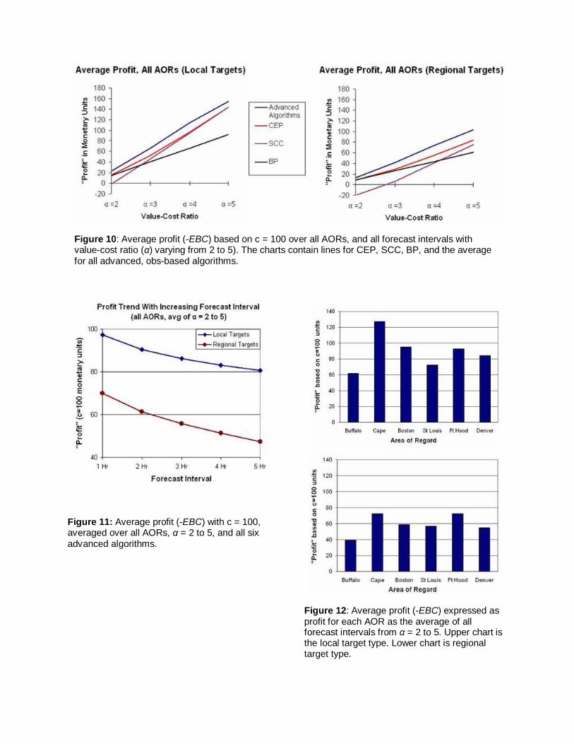
Figure 11: Average profit (-EBC) with c = 100, averaged over all AORs, α = 2 to 5, and all six advanced algorithms.

Figure 12: Average profit (-EBC) expressed as profit for each AOR as the average of all forecast intervals from α = 2 to 5. Upper chart is the local target type. Lower chart is regional target type.

Figure 10: Average profit (-EBC) based on c = 100 over all AORs, and all forecast intervals with value-cost ratio (α) varying from 2 to 5). The charts contain lines for CEP, SCC, BP, and the average for all advanced, obs-based algorithms.

e. Reliability Reliability is equivalent to bias and answers the question of how well the predicted probabilities of an event correspond to their observed frequencies. It complements ROC analysis and the EBC metric. To calculate reliability, probabilities output from each forecast algorithm were rounded to the nearest tenth and binned. All cases falling in each bin were examined to determine how many had an outcome of clear (E = 0). The observed frequency of clear was then computed from those cases. This was done for each (nearest tenth) bin in the interval [0,1]. A perfect result for a given bin occurs when the observed frequency of clear is equal to the nearest tenth forecast probability for that bin. The root mean square reliability error (RMSRE) was then computed as follows. Let Bi equal a bin for one of the nearest tenth probabilities in [0,1] such that the number of cases for that bin is greater than zero, and let O be the observed frequency of clear. O = [f(B1), f(B2),...,f(Bk)], k ≤ 11, where f(Bi) =

i

i

BB

in cases ofnumber total clear"" outcome with in cases ofnumber

If PCi denotes the actual probability of clear representing bin Bi, then:

2

1))((1 ii

k

iPCBf

kRMSRE

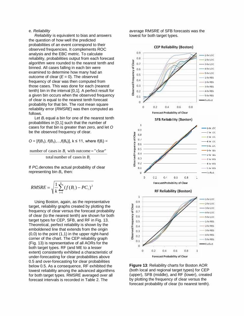
Using Boston, again, as the representative target, reliability graphs created by plotting the frequency of clear versus the forecast probability of clear (to the nearest tenth) are shown for both target types for CEP, SFB, and RF in Fig. 13. Theoretical, perfect reliability is shown by the emboldened line that extends from the origin (0,0) to the point (1,1) in the upper right-hand corner of the chart. The CEP reliability graph (Fig. 13) is representative of all AORs for the both target types. RF (and ME to a lesser extent) consistently exhibited a characteristic of under-forecasting for clear probabilities above 0.5 and over-forecasting for clear probabilities below 0.5. As a consequence, RF exhibited the lowest reliability among the advanced algorithms for both target types. RMSRE averaged over all forecast intervals is recorded in Table 2. The

average RMSRE of SFB forecasts was the lowest for both target types.

Figure 13: Reliability charts for Boston AOR (both local and regional target types) for CEP (upper), SFB (middle), and RF (lower), created by plotting the frequency of clear versus the forecast probability of clear (to nearest tenth).

Table 2: RMSRE for each obs-based algorithm, averaged over all forecast intervals for each target type in the Boston AOR. With regard to CEP, SFB, and RF, these data correspond to the reliability graphs in Fig. 13.

Average RMSRE, Boston

Local Regional ME 0.0302 0.0401 RF 0.0526 0.0583 NN 0.0170 0.0264 KAF 0.0281 0.0285 RT 0.0700 0.0446 SFB 0.0161 0.0197 CEP 0.0438 0.1328 SCC 0.1182 0.0202

7. DISCUSSION By testing the performance of multiple prediction algorithms across six weather regimes, this investigation makes a convincing case for the use of obs-based prediction algorithms for very short-range sky condition forecasting. As implemented, the RF and NN algorithms boasted the best overall performance. Only the linear combination of these two algorithms (ME) was able to exceed the performance of NN or RF, individually, with regard to certain performance metrics. In terms of overall performance as reflected by the ROC score and accuracy metrics, there was a small, but discernable advantage for all advanced algorithms over the baseline methods at 1-hr which grew with increasing forecast interval. Forecast accuracy decreased for all methods (except SCC) by ~7% on average between the 1- and 5-hr forecast intervals. This contrasts to the reduction in accuracy for BP of ~15% for both target types between the 1- and 5-hr forecasts. In terms of EBC, ME was the top performer for the local target type while NN was the top performer for the regional target type. EBC was a new value metric introduced for assessment of probabilistic forecasts by this investigation. SFB boasted the best reliability. However, all the advanced algorithms (i.e., KAF, RT, SFB, RF, and NN) were very reliable in all test trials. RF and ME were the only algorithms which showed any obvious bias. With regard to the baseline methods, CEP and BP performed comparably with respect to ROC score and accuracy. CEP, however, exceeded BP significantly in terms of EBC. This

advantage for CEP increased with increasing value-cost ratio, and with increasing forecast interval. This is due to the fact that CEP provides forecasts across the range of probabilities, while BP can only provide a probability of 0 or 100%, and is often wrong. In terms of EBC, SCC often outperformed BP (not shown) for value-cost ratio (α) ≥ ~3 and forecast intervals ≥ ~4. During the feature selection process, several of the METSAT-derived cloud structural features emerged as the strongest predictors. In many cases, a simple feature such as the percent areal coverage of cloud in the 100 x 100-km region surrounding the local target was the best predictor for multiple algorithms for a particular AOR, target type, and forecast interval. We believe that further research exploring feature development, selection and pruning are the most likely paths for increasing the performance results achieved in this investigation. In terms of feature development from METSAT, we have only just scratched the surface of possible cloud structural features, particularly in terms of better characterization of cloud morphology and temporal change in the cloud fields, and of making use of this information to enhance the predictions. For a global application of one or more of the algorithms presented in this paper, a CHANCES-class (Reinke et al. 2003), high spatial/temporal resolution satellite imagery, multi-year time series constructed from low-earth orbiting and geostationary weather satellites would be required. Additionally, imagery from future LEO satellites such as NPOESS would be needed to initialize analog queries for some geographic regions (e.g., polar). A concept for a global forecast system is described in a companion conference paper, Hall et al. (2010a). 8. ACKNOWLEDGEMENTS This work was sponsored by the NPOESS program under contract number DG133E07CQ0005. 9. REFERENCES Bankert, R. L, and M. Hadjimichael, 2007: Data mining numerical model output for single-station cloud-ceiling forecast algorithms. Wea. Forecasting, 22, 1123-1131.

Bellman, R. E., 1961: Adaptive control processes. Princeton University Press. 273 pp. Beyer, K., J. Goldstein, R. Ramakrishnan, and U. Shaft, 1999: “When Is `Nearest Neighbor' Meaningful?”, Proc. 7th International Conference on Database Theory, Jerusalem, Israel, Assoc. Comp. Machinery Spec. Int. Group on Man. of Data, 217-235. Black, T. L., 1994: The new NMC mesoscale Eta Model: Description and forecast examples. Wea. Forecasting, 9, 265-278. Breiman, L., 2001: Random forests. Machine Learning, 45, 5-32. Breiman, L., J. H. Friedman, R. A. Olshen, and C. J. Stone, 1998: Classification and regression trees. Chapman & Hall, 368 pp. Blanchard, D. O., and R. E. Lopez, 1985: Spatial patterns of convection in south Florida. Mon. Wea. Rev., 113, 1282-1299. Combs, C.L., W. Blier, W. Strach, M., DeMaria, 2004: Exploring the timing of fog formation and dissipation over San Francisco Bay area using satellite cloud composites. Preprints, 13th Conf. Satellite Meteorology and Oceanography, Norfolk, VA, Amer. Meteor. Soc. Connell, B. H., K. Gould, and J. F. W. Purdom, 2001: High-resolution GOES-8 visible and infrared cloud frequency composites over northern Florida during the summers 1996-1999. Wea. Forecasting, 16, 713-724. Duda, R. O. and P. E. Hart, 1973: Pattern classification and scene analysis. Wiley, 482 pp. Enger, I., L. J. Reed, and J. E. MacMonegle, 1962: An evaluation of 2-7-hr aviation terminal-forecasting techniques. Interim Report Technical Publication 20 prepared for the Federal Aviation Agency, Systems Research and Development Service by the Travelers Research Center Inc., 43 pp. Fukunaga, K., 1990: Introduction to Statistical Pattern Recognition. Academic Press, 592 pp. Girodo, M., R. W. Mueller, and D. Heinemann, 2006: Influence of three-dimensional cloud effects on satellite derived solar irradiance

estimation—first approaches to improve the Heliosat methods. Solar Energy, 80, 1145-1159. Gneiting, T., and R. Ranjan, 2008: Combining Probability Forecasts, Technical Report no. 543, Department of Statistics, University of Washington, 24 pp. Hall, T. J., D. L. Reinke, and T. H. Vonder Haar, 1998: Forecasting applications of high-resolution satellite cloud composite climatologies. Wea. Forecasting, 13, 16-23. Hall, T. J., R. N. Thessin, G. J. Bloy and C. N. Mutchler, 2009: Analog sky condition forecasting based on a k-nn algorithm. Submitted to Wea. Forecasting. Hall, T. J., C. N. Mutchler, and S. K. Gaffney, 2010a: Operational concept for observation-based forecasting of clear sky condition. 6th Annual Symp. of Future NPOESS and GOES-R, Atlanta, GA, Amer. Meteor. Soc. Hall, T. J., R. N. Thessin, G. J. Bloy, and C. N. Mutchler, 2010b: Comparison of artificial intelligence and statistical techniques for probabilistic forecasting of sky condition. 14th Conf. on Aviation, Range, and Aerospace Meteorology, Atlanta, GA, Amer. Meteor. Soc. Hansen, B., 2007: A fuzzy logic-based analog forecasting system for ceiling and visibility. Wea. Forecasting, 22, 1319-1330. Harvey, L. O. Jr., K. R. Hammond, C. M. Lusk, and E. F. Mross, 1992: The application of signal detection theory to weather forecasting behavior. Mon. Wea. Rev., 120, 863-883. Hu, M. J. C., 1964: Application of the adaline system to weather forecasting. Master’s thesis, Stanford Electronics Laboratories, Stanford, CA. Jedlovec, G. J., S. L. Haines, and F. J. LaFontaine, 2008: Spatial and temporal varying thresholds for cloud detection in GOES imagery. IEEE Trans. Geosci. Rem. Sens., 46, 1-13. Johns, M. V. 1961: An empirical Bayes approach to nonparametric two-way classification. Studies in item analysis and prediction, H. Soloman, ed., Stanford University Press, 221-232.

Kelly, F. P., 1988: Spatial and temporal short range total cloud cover estimation by metric analysis of composite imagery, Ph.D. dissertation, Department of Atmospheric Science, Colorado State University, Fort Collins, CO, 152 pp. Mason, S. J., and N. E. Graham, 2002: Areas beneath the relative operating characteristic (ROC) and relative operating levels (ROL) curves: Statistical significance and interpretation. Q. J. R. Meteorol. Soc., 128, 2145-2166. Mason, I., 1982: A model for assessment of weather forecasts. Aus. Met. Mag., 30, 291-303. Murphy, A. H., and M. Ehrendorfer, 1987: On the relationship between the accuracy and value of forecasts in the cost-loss ratio situation. Wea. Forecasting, 2, 243-251. Nabney, I. T., 2001: Netlab: Algorithms for Pattern Recognition. Springer, 438 pp. Norquist, D. C., 1999: Cloud predictions diagnosed from global weather model forecasts. Mon. Wea. Rev., 128, 3528-3555. Quinlan, J. R., 1986: Induction of decision trees. Machine Learning, 1, 81-106. Reinke, D. L., C. L. Combs, S. Q. Kidder and T. H. Vonder Haar, 1992: Satellite cloud composite climatologies: A new high-resolution tool in atmospheric research and forecasting. Bull. Amer. Meteor. Soc., 73, 278-285. Reinke, D. L., J. M. Forsythe, J. A. Kankiewicz, K. R. Dean, C. L. Combs, and T. H. Vonder Haar, 2003: Development and applications of regional cloud products from the CHANCES global cloud database. 12th Conf. on Satellite Meteorology and Oceanography, Long Beach, CA, Amer. Meteor. Soc. Sutton, C. D., 2005: Classification and regression trees, bagging, and boosting, Handbook of Statistics, 24, 303-329. Vislocky, R. L., and J. M. Fritsch, 1997: An automated, observation-based system for short-term prediction of ceiling and visibility. Wea. Forecasting, 12, 31-43.

Wettschereck, D., 1994: A study of distance-based machine learning algorithms. Doctoral dissertation, Oregon State University, Department of Computer Science. Witten, I. H., and E. Frank, 2005: Data Mining: Practical Machine Learning Tools and Techniques. Morgan Kaufmann, 560 pp. Zhang, G., B. E. Patuwo, and M. Y. Hu, 1998: Forecasting with artificial neural networks. Intl. J. Forecasting, 14, 35-62.