50th AIAA Aerospace Sciences Meeting including the New ...highorder.berkeley.edu/proceedings/aiaa-annual-2012/paper0332.pdf · and experimentally evaluated to analysis the particles

Development and Application of Nanoparticle Tracers for PIV in Supersonic and Hypersonic Flows

Fang Chen1, Hong Liu2 and Zhen Rong3

School of Aeronautics and Astronautics, Shanghai JiaoTong University, Shanghai 200240, China

The potential development and application of Nanoparticle tracers for supersonic and hypersonic flow diagnostics is investigated. The experiments are conducted in the Multi-Mach number high-speed wind tunnel (MMT) of SJTU, which has a test section of Φ200 mm with a Mach number range from 2.5 to 7. Nanoparticle tracers for PIV have been demonstrated to have a suitable flow tracking capability and high frequency response to record the high speed flows. Commonly used tracer materials and its size specifications are discussed and quantified for a wedge model in typically Mach number of 4 and 7, respectively. The results show that the application of nanoparticles as tracers is available for PIV to capture the flow structure at high spatiotemporal resolution in supersonic and hypersonic flow regimes. Moreover, tradeoff investigation may contribute to selecting appropriate particles for PIV at various freestream velocities.

Nomenclature

American Institute of Aeronautics and Astronautics

1

I. Introduction Particle Image Velocimetry (PIV) is among the most useful tools for flow diagnostics, which has the potential

to gain almost instantaneous velocity field with qualitative visualization and quantitative analysis. However, the application and accuracy of PIV requires suitable tracer particles, and depends on the time response. The flow tracking capability is particularly critical in extreme situation for the supersonic flow diagnostics with PIV[1]. Some issues about PIV applied to compressible flows were discussed by Moraitis[2] and Kompenhans[3] to record speed and seeding particle tracing accuracy. J. Haertig[4] conducted nozzle calibration measurements in shock tunnel at Mach 3.5 and 4.5. A challenging application of PIV was pioneered by Schrijer et al.[5] to investigate the flow over a double ramp configuration in a Mach 7 flow, produced by a Ludwieg tube facility. Measurements under the extreme high-speed conditions demand particles of still smaller relaxation time[6, 7]. Ragni et al.[8] have obtained the relaxation time of different solid particles and generation/filtration procedures based on an extensive investigation. Nanoparticles are desirable to secure sufficient detail in supersonic flow field. However, the scatter light declines with the power 6 of the particle diameter for sub-micron particles in Rayleigh scattering regime[6]. A solution to this problem may be to find a tradeoff selection of particle material and size in experimental investigation. The present work investigates the potential application of commonly used nanoparticle such as Al2O3 and TiO2 with different nominal diameters, seeded into the flow field for PIV. The flow tracking performance of the particles is theoretically

M∞ = freestream Mach number U∞ = freestream velocity Pt = total pressure Tt = total temperature μ = fluid dynamic viscosity Rex = Reynolds number per unit FOV = field of view Resolution = CCD resolution IA = interrogation area Up = particle velocity d = particle diameter

ρp = particle density ρ = fluid density τ = particle relaxation time up0 = particle initial velocity x = particle displacement ξ = particle relaxation distance upn = particle normal velocity un1 = fluid normal velocity before shock wave un2 = fluid normal velocity after shock wave U* = nondimensional particle (slip) velocity

p

1 Associate Professor, School of Aeronautics and Astronautics, 800 Dongchuan Road, Minhang District, Shanghai, 200240, China. 2 Professor, School of Aeronautics and Astronautics, 800 Dongchuan Road, Minhang District, Shanghai, 200240, China. 3 Post-Doc, School of Aeronautics and Astronautics, 800 Dongchuan Road, Minhang District, Shanghai, 200240, China.

50th AIAA Aerospace Sciences Meeting including the New Horizons Forum and Aerospace Exposition09 - 12 January 2012, Nashville, Tennessee

AIAA 2012-0036

Copyright © 2012 by the American Institute of Aeronautics and Astronautics, Inc. All rights reserved.

and experimentally evaluated to analysis the particles imaging. In the following sections, this paper will specify PIV and particle seeding system applied to MMT of SJTU. Finally, the suitability of the nanoparticles as tracers for PIV in supersonic and hypersonic flows is discussed.

II. Experimental Apparatus and Setup

A. Wind tunnel The experimental investigations are conducted in Multi-Mach number High-speed wind tunnel (MMT) of

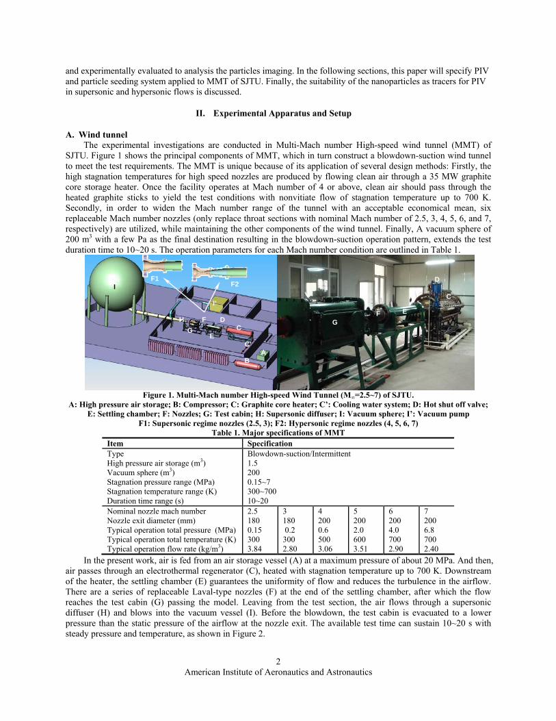
SJTU. Figure 1 shows the principal components of MMT, which in turn construct a blowdown-suction wind tunnel to meet the test requirements. The MMT is unique because of its application of several design methods: Firstly, the high stagnation temperatures for high speed nozzles are produced by flowing clean air through a 35 MW graphite core storage heater. Once the facility operates at Mach number of 4 or above, clean air should pass through the heated graphite sticks to yield the test conditions with nonvitiate flow of stagnation temperature up to 700 K. Secondly, in order to widen the Mach number range of the tunnel with an acceptable economical mean, six replaceable Mach number nozzles (only replace throat sections with nominal Mach number of 2.5, 3, 4, 5, 6, and 7, respectively) are utilized, while maintaining the other components of the wind tunnel. Finally, A vacuum sphere of 200 m3 with a few Pa as the final destination resulting in the blowdown-suction operation pattern, extends the test duration time to 10~20 s. The operation parameters for each Mach number condition are outlined in Table 1.


2

A

CE

B

DF G

H

I

I’

C’

F1 F2

C

E

D

F G

Figure 1. Multi-Mach number High-speed Wind Tunnel (M∞=2.5~7) of SJTU. A: High pressure air storage; B: Compressor; C: Graphite core heater; C’: Cooling water system; D: Hot shut off valve;

E: Settling chamber; F: Nozzles; G: Test cabin; H: Supersonic diffuser; I: Vacuum sphere; I’: Vacuum pump F1: Supersonic regime nozzles (2.5, 3); F2: Hypersonic regime nozzles (4, 5, 6, 7)

Table 1. Major specifications of MMT Item Specification Type High pressure air storage (m3) Vacuum sphere (m3) Stagnation pressure range (MPa) Stagnation temperature range (K) Duration time range (s)

Blowdown-suction/Intermittent 1.5 200 0.15~7 300~700 10~20

Nominal nozzle mach number Nozzle exit diameter (mm) Typical operation total pressure (MPa)Typical operation total temperature (K)Typical operation flow rate (kg/m3)

2.5 180 0.15 300 3.84

3 180 0.2 300 2.80

4 200 0.6 500 3.06

5 200 2.0 600 3.51

6 200 4.0 700 2.90

7 200 6.8 700 2.40

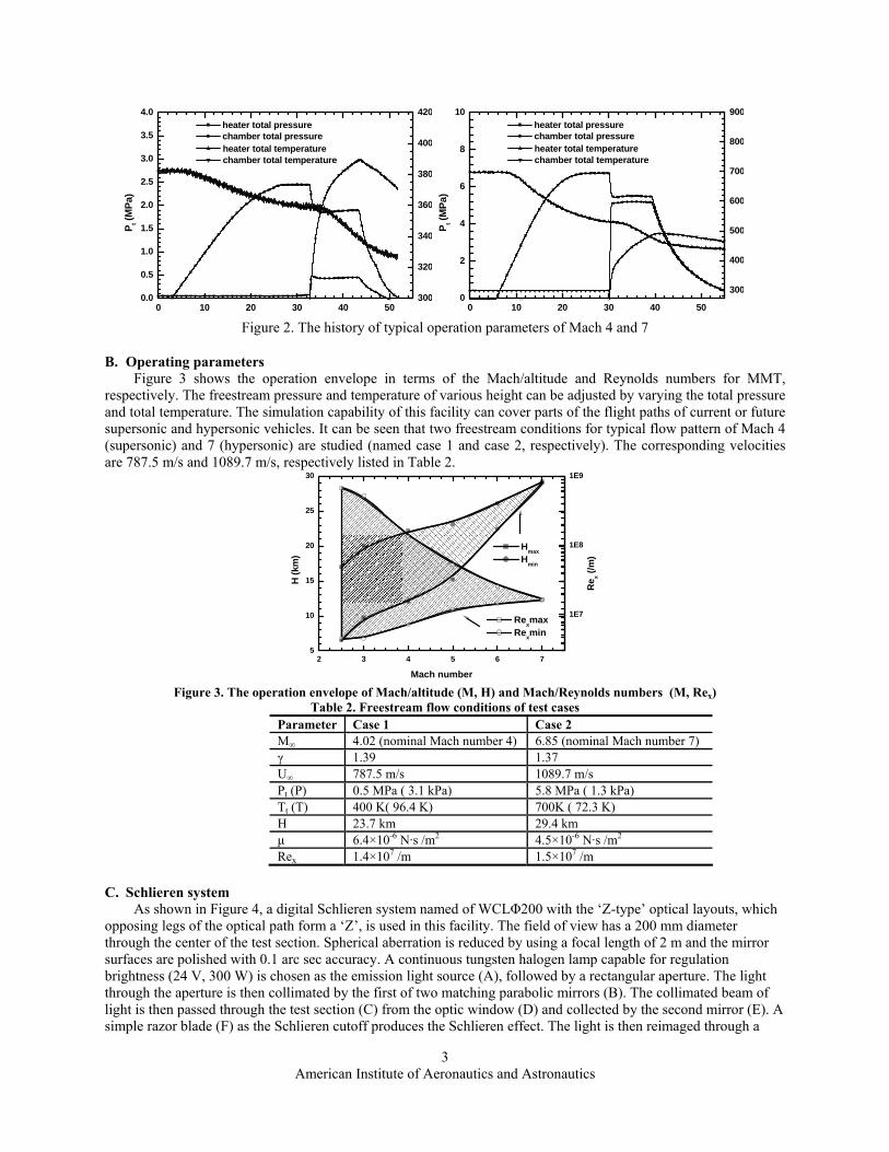
In the present work, air is fed from an air storage vessel (A) at a maximum pressure of about 20 MPa. And then, air passes through an electrothermal regenerator (C), heated with stagnation temperature up to 700 K. Downstream of the heater, the settling chamber (E) guarantees the uniformity of flow and reduces the turbulence in the airflow. There are a series of replaceable Laval-type nozzles (F) at the end of the settling chamber, after which the flow reaches the test cabin (G) passing the model. Leaving from the test section, the air flows through a supersonic diffuser (H) and blows into the vacuum vessel (I). Before the blowdown, the test cabin is evacuated to a lower pressure than the static pressure of the airflow at the nozzle exit. The available test time can sustain 10~20 s with steady pressure and temperature, as shown in Figure 2.

0 10 20 30 40 500.0

0.5

1.0

1.5

2.0

2.5

3.0

3.5

4.0

P t (M

Pa)

heater total pressure chamber total pressure

300

320

340

360

380

400

420

heater total temperature chamber total temperature

0 10 20 30 40 500

2

4

6

8

10

P t (MPa

)

heater total pressure chamber total pressure

300

400

500

600

700

800

900

heater total temperature chamber total temperature

Figure 2. The history of typical operation parameters of Mach 4 and 7

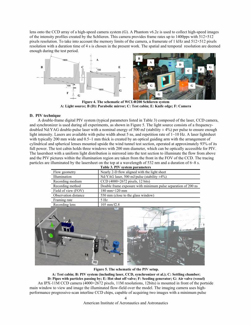
B. Operating parameters Figure 3 shows the operation envelope in terms of the Mach/altitude and Reynolds numbers for MMT,

respectively. The freestream pressure and temperature of various height can be adjusted by varying the total pressure and total temperature. The simulation capability of this facility can cover parts of the flight paths of current or future supersonic and hypersonic vehicles. It can be seen that two freestream conditions for typical flow pattern of Mach 4 (supersonic) and 7 (hypersonic) are studied (named case 1 and case 2, respectively). The corresponding velocities are 787.5 m/s and 1089.7 m/s, respectively listed in Table 2.

2 3 4 5 6 75

10

15

20

25

30

Re x (/

m)

H (k

m)

Mach number

Hmax Hmin

1E7

1E8

1E9

Rexmax Rexmin

Figure 3. The operation envelope of Mach/altitude (M, H) and Mach/Reynolds numbers (M, Rex)

Table 2. Freestream flow conditions of test cases Parameter Case 1 Case 2 M∞ 4.02 (nominal Mach number 4) 6.85 (nominal Mach number 7) γ 1.39 1.37 U∞ 787.5 m/s 1089.7 m/s Pt (P) 0.5 MPa ( 3.1 kPa) 5.8 MPa ( 1.3 kPa) Tt (T) 400 K( 96.4 K) 700K ( 72.3 K) H 23.7 km 29.4 km μ 6.4×10-6 N·s /m2 4.5×10-6 N·s /m2

Rex 1.4×107 /m 1.5×107 /m

C. Schlieren system As shown in Figure 4, a digital Schlieren system named of WCLΦ200 with the ‘Z-type’ optical layouts, which

opposing legs of the optical path form a ‘Z’, is used in this facility. The field of view has a 200 mm diameter through the center of the test section. Spherical aberration is reduced by using a focal length of 2 m and the mirror surfaces are polished with 0.1 arc sec accuracy. A continuous tungsten halogen lamp capable for regulation brightness (24 V, 300 W) is chosen as the emission light source (A), followed by a rectangular aperture. The light through the aperture is then collimated by the first of two matching parabolic mirrors (B). The collimated beam of light is then passed through the test section (C) from the optic window (D) and collected by the second mirror (E). A simple razor blade (F) as the Schlieren cutoff produces the Schlieren effect. The light is then reimaged through a


3

lens onto the CCD array of a high-speed camera system (G). A Phantom v6.2e is used to collect high-speed images of the intensity profiles created by the Schlieren. This camera provides frame rates up to 1400pps with 512×512 pixels resolution. To take into account the memory limits of the camera, a framerate of 1 kHz and 512×512 pixels resolution with a duration time of 4 s is chosen in the present work. The spatial and temporal resolution are deemed enough during the test period.


4

Figure 4. The schematic of WCLΦ200 Schlieren system

A: Light source; B (D): Parabolic mirror; C: Test cabin; E: Knife edge; F: Camera

D. PIV technique A double-frame digital PIV system (typical parameters listed in Table 3) composed of the laser, CCD camera,

and synchronizer is used during all experiments, as shown in Figure 5. The light source consists of a frequency-doubled Nd:YAG double-pulse laser with a nominal energy of 500 mJ (stability ± 4%) per pulse to ensure enough light intensity. Lasers are available with pulse width about 5 ns, and repetition rate of 1~10 Hz. A laser lightsheet with typically 200 mm wide and 0.5~1 mm thick is created by an optical guiding arm with the arrangement of cylindrical and spherical lenses mounted upside the wind tunnel test section, operated at approximately 93% of its full power. The test cabin holds three windows with 200 mm diameter, which can be optically accessible for PIV. The lasersheet with a uniform light distribution is mirrored into the test section to illuminate the flow from above and the PIV pictures within the illumination region are taken from the front in the FOV of the CCD. The tracing particles are illuminated by the lasersheet on the top at a wavelength of 532 nm and a duration of 6~8 s.

Table 3. PIV system parameters Flow geometry Nearly 2-D flow aligned with the light sheet Illumination Nd:YAG laser, 500 mJ/pulse (stability ±4%) Recording medium CCD (4000×2672 pixels, 12 bits) Recording method Double frame exposure with minimum pulse separation of 200 ns Field of view (FOV) 180 mm×120 mm Observation distance 550 mm (close to the glass window) Framing rate 5 Hz Recording lens 105 mm/f2.8

Figure 5. The schematic of the PIV setup.

A: Test cabin; B: PIV system (including laser, CCD, synchronizer et al.); C: Settling chamber; D: Pipes with particles passing by; E: Hot shut off valve; F: Seeding generator; G: Air valve (vessel)

An IPX-11M CCD camera (4000×2672 pixels, 11M resolutions, 12bits) is mounted in front of the portside main window to view and image the illuminated flow-field over the model. The imaging camera uses high-performance progressive-scan interline CCD chips, capable of acquiring two images with a minimum pulse

BA

C

D G

F

G G

G

1900

100

100

1900

B

A

C

GF

G

E

A

B

separation of 200 ns and framing rate of 5 Hz. The pulse separation (dT) is a critical parameter, which is the time between the fringe of A Q-Switch and B Q-Switch, for matching the PIV system to the flow velocity. It is the preferred method in conjunction with special triggering options for synchronizing the measurements to capture high speed flow. An optimized pulse separation value should be chosen to lead to good measurement. The particle images are recorded at 5 Hz resulting in 50~100 image pairs per tunnel run. A 105 mm SIGMA objective at f=2.8 is carefully chosen to modify the field of view and avoid dim particle images with sufficient collected energy. The camera is fitted with a narrowband-pass 532 nm filter to minimize ambient light interference.

Synchronization between the cameras, laser, and image acquisition is accomplished by a programmable timing unit. The synchronizer separation time is checked by a fast-response photodiode and timing errors were found to be less than 1%. Figure 6 shows the timing diagrams of laser pulse and CCD to synchronize the illumination and image acquisition. The CCD shutter is triggered by synchronizer signal and the feedback signal of CCD is transferred back to the synchronizer. By utilizing double exposure technique of CCD, the instantaneous structure of high speed flow can be captured to study the temporal evolution of the flow field, while setting the timing diagrams according to the mainflow velocity.


5

0T 1 T 2 T 3 T 4 T 5 T 6 T 7 T 8

D e la y 1

D e la y 2

D e la y 3

D e la y 4

D e la y 7

D e la y X

D e la y 6

D e la y 5

T 0C C D T r ig g e r

C C D E x p o s a l

A L a m p T rig g e r

A Q -S W T r ig g e r

A L a s e r O u tp u t

B L a m p T rig g e r

B Q -S W T r ig g e r

B L a s e r O u tp u t

Figure 6. The timing diagrams of PIV. The association of double exposure CCD and double pulse laser makes it possible to apply PIV to supersonic

and hypersonic flows. The most common algorithm by far while neglecting the other parameters and adaptive correlation method, can be written as

solutionRedT4IAFOVU

⋅⋅⋅

= (1)

where FOV is the field of view, Resolution is specific to the CCD resolution, and IA is the selected interrogation area. Therefore, the desired dT for Case 1(787.5 m/s, nominal Mach number of 4) and Case 2 (1089.7 m/s, nominal Mach number of 7) in the present work can be approximately estimated at 500 ns and 400 ns, respectively.

The PIV images are analyzed after the experiment by a FFT based cross-correlation algorithm of Micro Vec2 software with adaptive interrogation window sizes. The averaging analysis of the cross-correlation images over the available ensemble of recordings is carried out to enhance the reliability of the measurement under intermittent seeding conditions. Raw PIV images of the tracer particles are captured by PIV system in a grayscale format. In order to examine individual particles, the images must be converted to black and white by means of Micro Vec2. Pixels identified as background noise are set to black, while pixels showing light scattered off a particle are set to white, thus easier discerning individual particles. The details of the same image over a wedge in Case 1 before and after processing are shown in Figure 7.

Figure 7. PIV images before and after processing

III. Particles Selection and Seeding

A. Motion of tracer particles in flows It is clear from the principle of PIV that this technique is based on images of tracer particles suspending in the

flow. In an ideal situation, these tracer particles in the flow should not only follow all flow velocity fluctuations but are also sufficient in number to provide the desired spatial or temporal resolution of the measured flow velocity. In that case, the local fluid velocity can be instead of the particles displacement from multiple particles images dividing their moving time, i.e. the time interval. From the general issues of tracer particles in Melling[9], if only the viscous and inertia terms are considered, the difference between the particle velocity Up and that of the surrounding fluid U to be estimated as

dt

dU18

dUU pp2pp μ

ρρ −−=− (2)

where μ is the dynamic viscosity of the flow and dp is the diameter of the particle. As for solid tracer particles in gas flows, the density of the particle ρp is much greater than the fluid density ρ, then the particles can never accurately follow the flow. In the case that ρp»ρ (gas flows), the particles response to a stepwise variation in the flow velocity typically follows an exponential decay law:

⎥⎦

⎤⎢⎣

⎡⎟⎠⎞

⎜⎝⎛−−=

τtexp1U)t(U p (3)

with the relaxation time τ given by:

μρ

τ18

d p2p= (4)

Then integrating Equation (3) over the time range of [0, t] results in

⎟⎠⎞

⎜⎝⎛−=

−

−

τtexp

UUUU

0p

p (5)

and

τ1

UUUU

dtd

0t0p

p −=⎟⎟⎠

⎞⎜⎜⎝

⎛

−

−

=

(6)

It means that while a particle with initial velocity up0 is seeded into the flow, the particle will accelerate with the surrounding flow at the rate of 1/τ. The corresponding velocity Up is gradually increase close to, but never up to the flow velocity U. Equation (3) is further integrated over the time range of [0, t] to obtain the particle displacement, x, as a function of time:

⎥⎦

⎤⎢⎣

⎡−⎟

⎠⎞

⎜⎝⎛−+= 1texpUUtx

ττ (7)

The relaxation distance ξ of a particle in a continuously accelerating flow is derived by substituting t=τ, eUτξ = (8)

Now, a nondimensional velocity U*, i.e. slip velocity of a particle is defined as (Up–U)/(Up0–U). The present work has done the effort to analysis the relaxation process. By using Equation (5) and (7), the velocity gradually increases with the increasing displacement:

( ) ( )∗∗

∗

−−=

⎥⎦

⎤⎢⎣

⎡⎟⎠⎞

⎜⎝⎛−−

⎟⎠⎞

⎜⎝⎛−

−=U1U

Utexp1U

texpU

dxd

ττ

τ

τ (9)

By integrating Equation (9), the particle displacement is obtained as follows: [ ]1UlnUUx −−= ∗∗τ (10)


6

[ ]1UlnUex−−= ∗∗

ξ (11)

Therefore, the time interval should be smaller than the flow time scale to avoid significant discrepancy between fluid and particle motion, then getting an approximate instantaneous flow velocity. The velocity gradient of the tracking particle will be desired in the present work when

2lnt ⋅= τ (12) The resulting relationship can easily calculate the relaxation time, which is determined by the particle diameters

from Equation (4). Such a simple criterion may contribute to selecting appropriate particles to attain velocity equilibrium with flow. For a given time interval t=dT, i.e. the pulse separation time, 500 ns (Case 1) and 400 ns (Case 2) recommended from Equation (1), The diameter of the typical particles of titanium dioxide (TiO2, density ρp is generally 4.23×103 kg/m3) obtained should be 150 nm (Case 1) and 120 nm (Case 2) to ensure good tracking of supersonic flow. In other words, the selection of nanoparticles is critical for the successful application of PIV to supersonic and hypersonic regime.

Moreover in high-speed flows, especially within limited regions downstream of shock waves, where the flow decelerates abruptly the particle tracers. The particles follow the actual flow streamlines with a decelerate/relax process to the flow velocity downstream of the shock wave in a finite time instead of a discontinuity at the shock location. The tracer particles decelerate with an exponential decay, similar to Equation (5):

⎟⎠⎞

⎜⎝⎛−=

−

−

τtexp

UUUU

2n1n

2npn (13)

where upn is specific to the normal velocity of the particle, un1 and un2 represent the normal velocity of the flow before and after the shock wave. Further information regarding the response of particles across shock waves can be found in Dring[10] or Tedeschi et al.[11] Such a procedure was adopted in previous investigation[4, 12-14] to obtain the velocity profile across a planar oblique shock wave, following the fact that the particle velocity profile normal to the shock wave where the tracer particles decelerate gradually due to inertia[15].

The measurement of the nondimensional particle (slip) velocity U*=(Upn–Un2)/(Un1–Un2) showed a smoothing effect of the velocity profile at the shock location, which can quantify the particle location normal to the shock wave, xn, as a function of the relaxation distance ξn derived from Equation (7) and (11):

( ) [ ]1UUUtUx 2n1n2nn −−+= ∗τ (14)

[ ]1UlnUex

n

n −−= ∗∗

ξ (15)

where the particle relaxation distance ( )[ ]eUUU 2n1n1nn −−=τξ (16)

The particles decelerate to the flow velocity downstream of the shock wave in a relaxation process, which velocity time history does not exhibit a discontinuity at shock location. In case that supersonic tests conducted over the wedge with a small deflection angle[16-17], the normal Mach number is typically lower than 1.4, Equations (13) and (14) can be approximated by a linear relationship. Therefore,

n

nxtUlnξτ

−≈−=∗ (17)

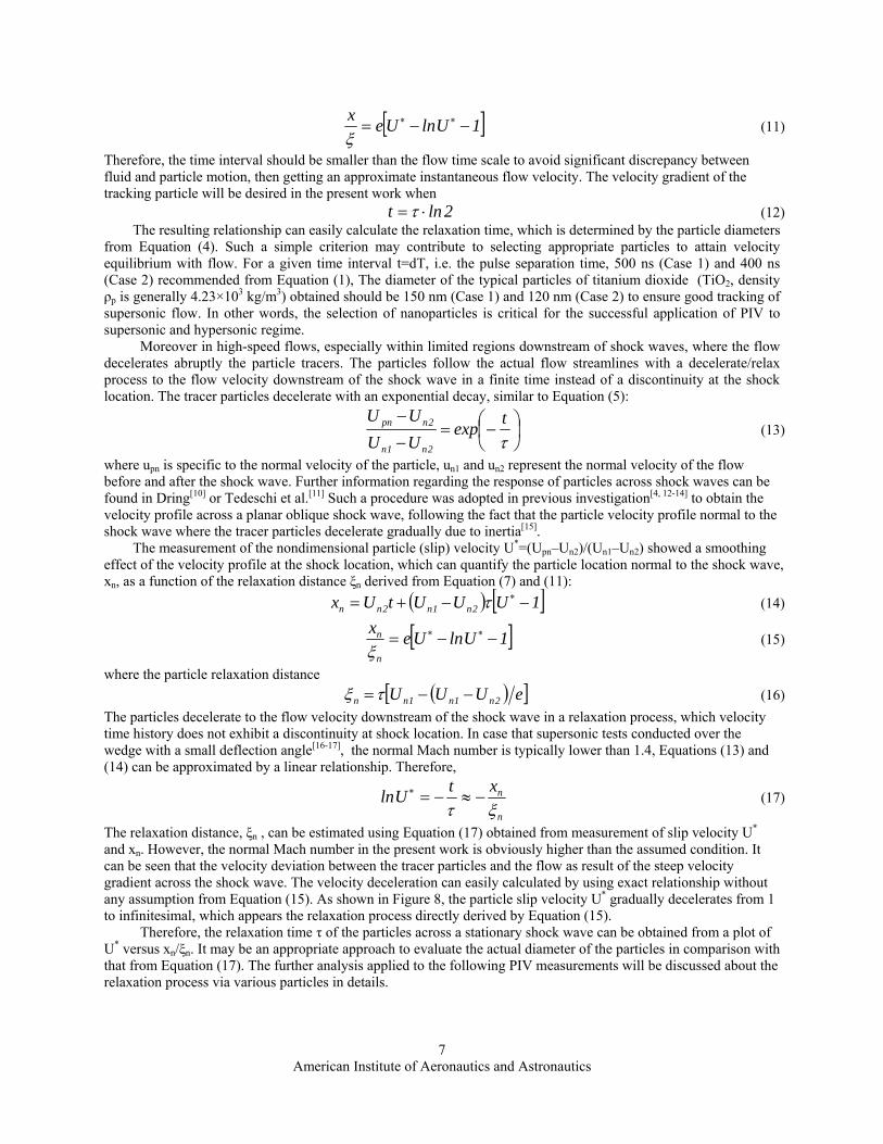
The relaxation distance, ξn , can be estimated using Equation (17) obtained from measurement of slip velocity U* and xn. However, the normal Mach number in the present work is obviously higher than the assumed condition. It can be seen that the velocity deviation between the tracer particles and the flow as result of the steep velocity gradient across the shock wave. The velocity deceleration can easily calculated by using exact relationship without any assumption from Equation (15). As shown in Figure 8, the particle slip velocity U* gradually decelerates from 1 to infinitesimal, which appears the relaxation process directly derived by Equation (15).

Therefore, the relaxation time τ of the particles across a stationary shock wave can be obtained from a plot of U* versus xn/ξn. It may be an appropriate approach to evaluate the actual diameter of the particles in comparison with that from Equation (17). The further analysis applied to the following PIV measurements will be discussed about the relaxation process via various particles in details.


7


8

-5 0 5 10-0.2

0.0

0.2

0.4

0.6

0.8

1.0

1.2

ξn

[1,1/e] Particle velocityFlow velocity

U*

xn/ξn

xn/ξn=e[U*-ln(U*)-1]

Figure 8. Relaxation process of particles across a shock wave

B. Particles material and size selection PIV provides indirect characterization of the fluid velocity through measurement of the velocity of the

suspended tracer particles. The fact that adding particles should be small enough to be good flow tracers and large enough to improve the scattering signal quality. These particles should also be healthy, safe, noncrrosive, and chemically inert. Finally, seeding material is expected to leaving minimum residues result from less contamination if possible. Among the requirements for the choice of the seeding material, extensive investigation has been conducted in PIV experiments[9, 18].

In cases where the stability of the seeding material cannot be guaranteed due to increased temperatures or reactive environments, seeding based on solids must be used. Metal oxide powders are especially well suited for this purpose due to their inertness, high melting point and rather low cost. Aluminum oxide (Al2O3), silicon dioxide (SiO2), and titanium dioxide (TiO2) powders are some of the most commonly used materials for high speed application, which properties are listed in Table 4.

Table 4. Commonly used solid tracer particles for PIV experiments Material Diameter (μm) Density (×103 kg/m3) Comments

Al2O3 0.2~1 3.95~4.1 Useful for seeding flames with high melting point 2300K

SiO2 0.2~1 2.65 Spherical particles with a very narrow size distribution. Better light scatterer than TiO2, lower melting point of 1900K

TiO2 0.01~1 4.23 Good light scattering and stable in flames up to 2800KVery wide size distribution and lumped particle shapes

As mentioned before, shorter relaxation times have traditionally been aimed at by applying smaller particles. For particles in nanometer size range, a rule of thumb is that agglomeration serves to increase the effective particle size by about an order of magnitude. Therefore, to achieve the submicron sizes desired in the test cabin, it is necessary to specify the ultra-fine powder. In the previous work, the 30 nm Al2O3 and TiO2 particles are used in the comparison experiments. By utilization Equation (4), the relaxation time of the particles for Case 1 is estimated to be almost same, 31 ns for the Al2O3 and 33 ns for the TiO2 respectively. These measurements agree well with the scattering based investigations[15, 19-20].

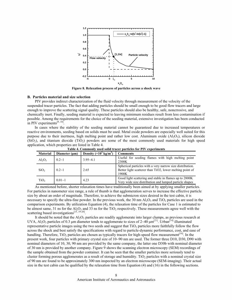
It should be noted that the Al2O3 particles are readily agglomerate into larger clumps, as previous research at UVA, Al2O3 particles of 0.3 μm diameter tends to agglomerate to sizes of 2~40 μm[21]. Urban[14] illuminated representative particle images using the two seeds and suggest that TiO2 particles more faithfully follow the flow across the shock and best satisfy the specifications with regard to particle-dynamic performance, cost, and ease of handling. Therefore, TiO2 particles are chosen as typically tracers for high-speed flow measurement[16]. In the present work, four particles with primary crystal size of 10~90 nm are used. The former three D10, D30, D90 with nominal diameters of 10, 30, 90 nm are provided by the same company, the latter one D30b with nominal diameter of 30 nm is provided by another company. Figure 9 shows the scanning electron microscopy (SEM) recordings of the sample obtained from the powder container. It can be seen that the smaller particles more seriously tend to cluster forming porous agglomerates as a result of storage and humidity. TiO2 particles with a nominal crystal size of 90 nm are found to be approximately 300 nm inspected by an electron microscope (SEM-imaging). Their actual size in the test cabin can be qualified by the relaxation time from Equation (4) and (16) in the following sections.


9

Figure 9. Micrographs of titanium dioxide powder used in the presented PIV applications

a b c d

Nominal 10 30 90 30b

C. Scattering properties of tracer particles Here the use of sub-micron or nano particles should be considered to fulfill the fluid-mechanical requirements

of tracers, but this would have the effect of a significant decrease in light scattering efficiency of the particles (Rayleigh scattering regime). The particle diameter dp is much smaller than the wavelength of light, dp«λ, the amount of light scattered by a particle varies as dp

−6[22]. This places significant constraints on the image recording optics, making it extremely difficult to record particle images. One solution to this imaging problem is to use a double-cavity Nd:YAG laser with higher energy to illuminate the seeding particles, resulting in enough light scattered from the particles to be visible. To minimize the reflections, illumination was almost tangent to the wall.

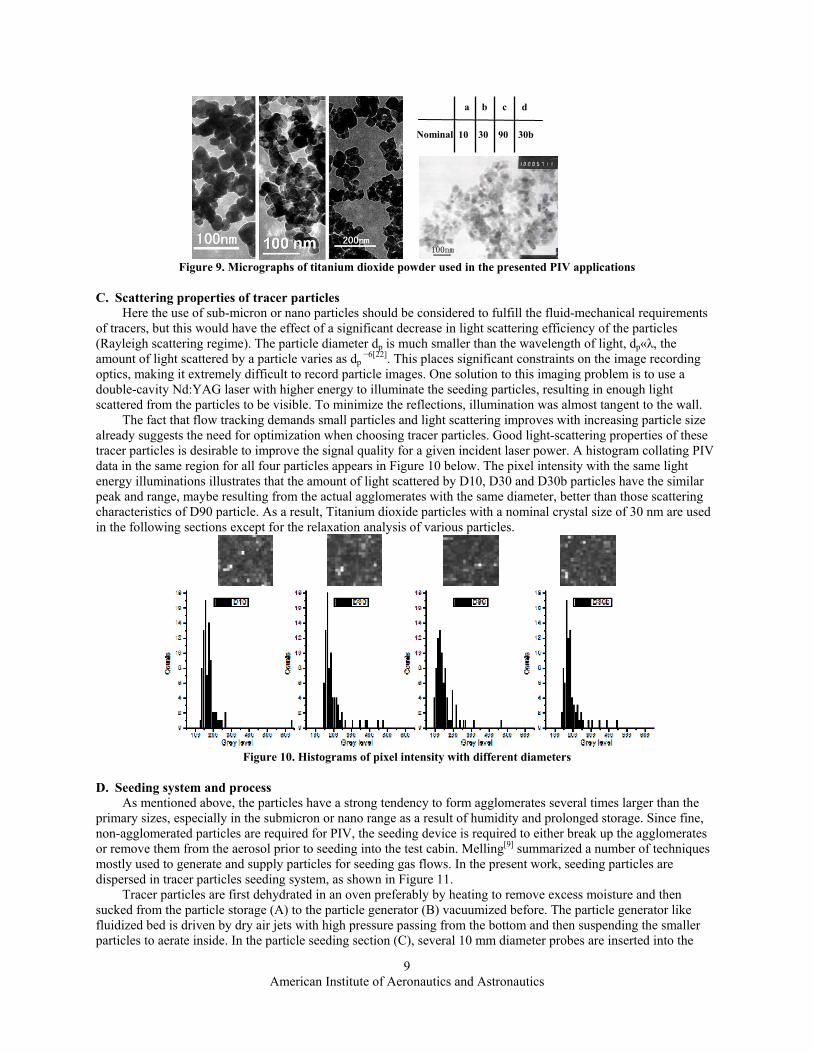
The fact that flow tracking demands small particles and light scattering improves with increasing particle size already suggests the need for optimization when choosing tracer particles. Good light-scattering properties of these tracer particles is desirable to improve the signal quality for a given incident laser power. A histogram collating PIV data in the same region for all four particles appears in Figure 10 below. The pixel intensity with the same light energy illuminations illustrates that the amount of light scattered by D10, D30 and D30b particles have the similar peak and range, maybe resulting from the actual agglomerates with the same diameter, better than those scattering characteristics of D90 particle. As a result, Titanium dioxide particles with a nominal crystal size of 30 nm are used in the following sections except for the relaxation analysis of various particles.

Figure 10. Histograms of pixel intensity with different diameters

D. Seeding system and process As mentioned above, the particles have a strong tendency to form agglomerates several times larger than the

primary sizes, especially in the submicron or nano range as a result of humidity and prolonged storage. Since fine, non-agglomerated particles are required for PIV, the seeding device is required to either break up the agglomerates or remove them from the aerosol prior to seeding into the test cabin. Melling[9] summarized a number of techniques mostly used to generate and supply particles for seeding gas flows. In the present work, seeding particles are dispersed in tracer particles seeding system, as shown in Figure 11.

Tracer particles are first dehydrated in an oven preferably by heating to remove excess moisture and then sucked from the particle storage (A) to the particle generator (B) vacuumized before. The particle generator like fluidized bed is driven by dry air jets with high pressure passing from the bottom and then suspending the smaller particles to aerate inside. In the particle seeding section (C), several 10 mm diameter probes are inserted into the

tube upstream of settling chamber (D) to seeding toward the exit orifice. The particles are injected into the mainflow and fully mixed in the test cabin to ensure ample and uniform seeding.


10

B

A C

D

E

Figure 11. Tracer particle seeding system. A: particle storage; B: particle generator with high pressure; C: particle seeding section; D: settling chamber; E: valve

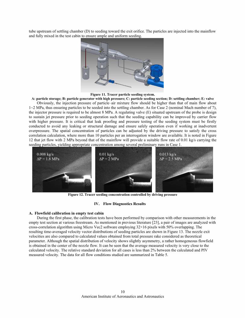
Obviously, the injection pressure of particle–air mixture flow should be higher than that of main flow about 1~2 MPa, thus ensuring particles to be seeded into the settling chamber. As for Case 2 (nominal Mach number of 7), the injector pressure is required to be almost 8 MPa. A regulating valve (E) situated upstream of the probe is design to sustain jet pressure prior to seeding operation such that the seeding capability can be improved by carrier flow with higher pressure. It is critical that leak proofing and pressure testing of the seeding system must be firstly conducted to avoid any leaking or structural damage and ensure safely operation even if working at inadvertent overpressure. The spatial concentration of particles can be adjusted by the driving pressure to satisfy the cross correlation calculation, where more than 10 particles per an interrogation window are available. It is noted in Figure 12 that jet flow with 2 MPa beyond that of the mainflow will provide a suitable flow rate of 0.01 kg/s carrying the seeding particles, yielding appropriate concentration among several preliminary runs in Case 1.

Figure 12. Tracer seeding concentration controlled by driving pressure

0.008 kg/s ∆P = 1.8 MPa

0.01 kg/s ∆P = 2 MPa

0.013 kg/s ∆P = 2.5 MPa

IV. Flow Diagnostics Results

A. Flowfield calibration in empty test cabin During the first phase, the calibration tests have been performed by comparison with other measurements in the

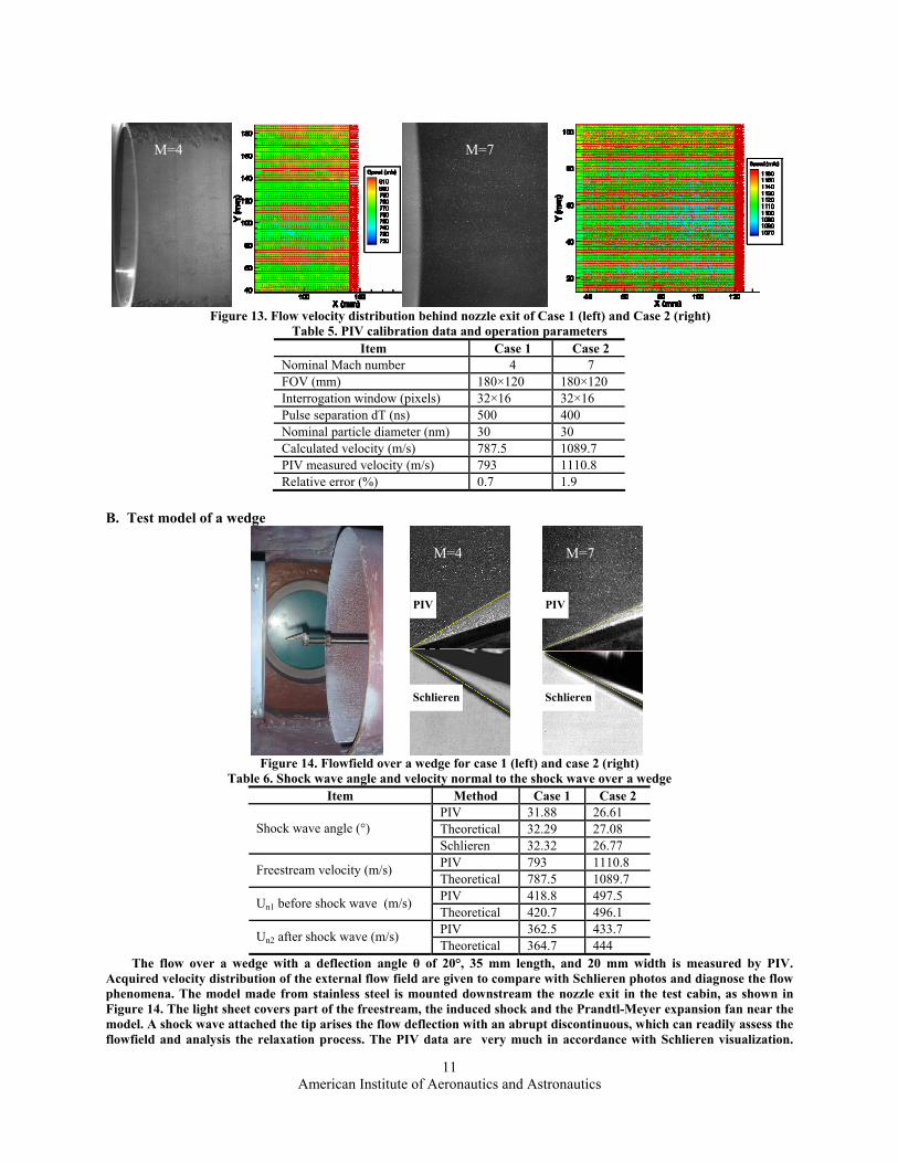
empty test section at various freestream. As mentioned in previous literature [23], a pair of images are analyzed with cross-correlation algorithm using Micro Vec2 software employing 32×16 pixels with 50% overlapping. The resulting time-averaged velocity vector distributions of seeding particles are shown in Figure 13. The nozzle exit velocities are also compared to calculated values obtained from total pressure rake considered as theoretical parameter. Although the spatial distribution of velocity shows slightly asymmetry, a rather homogeneous flowfield is obtained in the center of the nozzle flow. It can be seen that the average measured velocity is very close to the calculated velocity. The relative standard deviation for all cases is less than 2% between the calculated and PIV measured velocity. The data for all flow conditions studied are summarized in Table 5.


11

Figure 13. Flow velocity distribution behind nozzle exit of Case 1 (left) and Case 2 (right)

M=4 M=7

Table 5. PIV calibration data and operation parameters Item Case 1 Case 2

Nominal Mach number 4 7 FOV (mm) 180×120 180×120 Interrogation window (pixels) 32×16 32×16 Pulse separation dT (ns) 500 400 Nominal particle diameter (nm) 30 30 Calculated velocity (m/s) 787.5 1089.7 PIV measured velocity (m/s) 793 1110.8 Relative error (%) 0.7 1.9

B. Test model of a wedge

PIV

Schlieren

M=7

PIV

Schlieren

M=4

Figure 14. Flowfield over a wedge for case 1 (left) and case 2 (right)

Table 6. Shock wave angle and velocity normal to the shock wave over a wedge Item Method Case 1 Case 2

PIV 31.88 26.61 Theoretical 32.29 27.08 Shock wave angle (°) Schlieren 32.32 26.77 PIV 793 1110.8 Freestream velocity (m/s) Theoretical 787.5 1089.7 PIV 418.8 497.5 Un1 before shock wave (m/s) Theoretical 420.7 496.1 PIV 362.5 433.7 Un2 after shock wave (m/s) Theoretical 364.7 444

The flow over a wedge with a deflection angle θ of 20°, 35 mm length, and 20 mm width is measured by PIV. Acquired velocity distribution of the external flow field are given to compare with Schlieren photos and diagnose the flow phenomena. The model made from stainless steel is mounted downstream the nozzle exit in the test cabin, as shown in Figure 14. The light sheet covers part of the freestream, the induced shock and the Prandtl-Meyer expansion fan near the model. A shock wave attached the tip arises the flow deflection with an abrupt discontinuous, which can readily assess the flowfield and analysis the relaxation process. The PIV data are very much in accordance with Schlieren visualization.

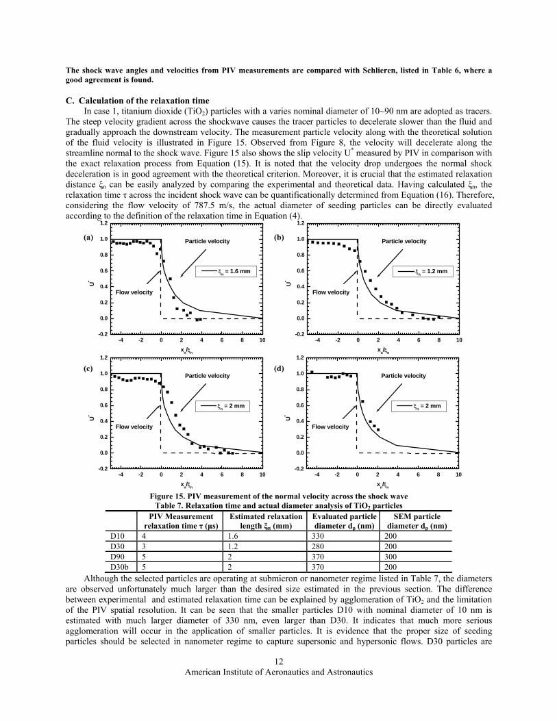
The shock wave angles and velocities from PIV measurements are compared with Schlieren, listed in Table 6, where a good agreement is found.

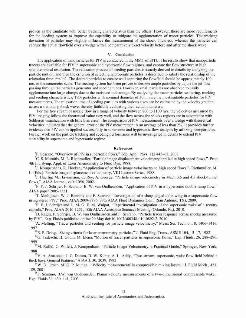
C. Calculation of the relaxation time In case 1, titanium dioxide (TiO2) particles with a varies nominal diameter of 10~90 nm are adopted as tracers.

The steep velocity gradient across the shockwave causes the tracer particles to decelerate slower than the fluid and gradually approach the downstream velocity. The measurement particle velocity along with the theoretical solution of the fluid velocity is illustrated in Figure 15. Observed from Figure 8, the velocity will decelerate along the streamline normal to the shock wave. Figure 15 also shows the slip velocity U* measured by PIV in comparison with the exact relaxation process from Equation (15). It is noted that the velocity drop undergoes the normal shock deceleration is in good agreement with the theoretical criterion. Moreover, it is crucial that the estimated relaxation distance ξn can be easily analyzed by comparing the experimental and theoretical data. Having calculated ξn, the relaxation time τ across the incident shock wave can be quantificationally determined from Equation (16). Therefore, considering the flow velocity of 787.5 m/s, the actual diameter of seeding particles can be directly evaluated according to the definition of the relaxation time in Equation (4).


12

-4 -2 0 2 4 6 8 10-0.2

0.0

0.2

0.4

0.6

0.8

1.0

1.2

Particle velocity

Flow velocity

U*

xn/ξn

ξn = 1.6 mm

-4 -2 0 2 4 6 8 10-0.2

0.0

0.2

0.4

0.6

0.8

1.0

1.2

Particle velocity

Flow velocityU

*

xn/ξn

ξn = 1.2 mm

-4 -2 0 2 4 6 8 10-0.2

0.0

0.2

0.4

0.6

0.8

1.0

1.2

Particle velocity

Flow velocity

U*

x

Figure 15. PIV measurement of the normal velocity across the shock wave Table 7. Relaxation time and actual diameter analysis of TiO2 particles

PIV Measurement relaxation time τ (μs)

Estimated relaxation length ξn (mm)

Evaluated particlediameter dp (nm)

SEM particle diameter dp (nm)

D10 4 1.6 330 200 D30 3 1.2 280 200 D90 5 2 370 300 D30b 5 2 370 200

Although the selected particles are operating at submicron or nanometer regime listed in Table 7, the diameters are observed unfortunately much larger than the desired size estimated in the previous section. The difference between experimental and estimated relaxation time can be explained by agglomeration of TiO2 and the limitation of the PIV spatial resolution. It can be seen that the smaller particles D10 with nominal diameter of 10 nm is estimated with much larger diameter of 330 nm, even larger than D30. It indicates that much more serious agglomeration will occur in the application of smaller particles. It is evidence that the proper size of seeding particles should be selected in nanometer regime to capture supersonic and hypersonic flows. D30 particles are

n n/ξ

ξn = 2 mm

-4 -2 0 2 4 6 8 10-0.2

0.0

0.2

0.4

0.6

0.8

1.0

1.2

Particle velocity

Flow velocity

ξn = 2 mm

(a) (b)

(c) (d)

U*

x /ξn n


13

proven as the candidate with better tracking characteristics than the others. However, there are more requirements for the seeding system to improve the capability to mitigate the agglomeration of tracer particles. The tracking deviation of particles may slightly influence the measurement of the shock thickness, whereas the particles can capture the actual flowfield over a wedge with a comparatively exact velocity before and after the shock wave.

V. Conclusion The application of nanoparticles for PIV is conducted in the MMT of SJTU. The results show that nanoparticle

tracers are available for PIV in supersonic and hypersonic flow regimes, and capture the flow structure at high spatiotemporal resolution. The relaxation process of seeding particles is exactly derived in details by analyzing the particle motion, and then the criterion of selecting appropriate particles is described to satisfy the relationship of the relaxation time: τ=t/ln2. The desired particles to ensure well capturing the flowfield should be approximately 100 nm, in the nanometer scale. The seeding system has been proven to despise ample particles by adjust the jet flow passing through the particles generator and seeding tubes. However, small particles are observed to easily agglomerate into large clumps due to the moisture and storage. By analyzing the tracer particles scattering, tracking and seeding characteristics, TiO2 particles with nominal diameter of 30 nm are the most suitable particles for PIV measurements. The relaxation time of seeding particles with various sizes can be estimated by the velocity gradient across a stationary shock wave, thereby faithfully evaluating their actual diameters.

For the free stream of nozzle flow in a range of velocity between 800 to 1100 m/s, the velocities measured by PIV imaging follow the theoretical value very well, and the flow across the shocks regions are in accordance with Schlieren visualization with little bias error. The comparison of PIV measurements over a wedge with theoretical velocities indicates that the general error of the PIV measurement is an average of less than 2%. It provides further evidence that PIV can be applied successfully in supersonic and hypersonic flow analysis by utilizing nanoparticles. Further work on the particle tracking and seeding performance will be investigated in details to extend PIV suitability in supersonic and hypersonic regime.

References 1F. Scarano, “Overview of PIV in supersonic flows,” Top. Appl. Phys. 112 445–63, 2008. 2C. S. Moraitis, M. L. Riethmuller, “Particle image displacement velocimetry applied in high speed flows,”. Proc.

4th Int. Symp. Appl. of Laser Anemometry to Fluid Dyn, 1988. 3J. Kompenhans, R. Hocker., “Application of particle image velocimetry to high speed flows,”. Riethmuller, M.

L. (Eds.): Particle image displacement velocimetry, VKI Lecture Series, 1988. 4J. Haertig, M. Havermann, C. Rey, A. George, “Particle image velocimetry in Mach 3.5 and 4.5 shock-tunnel

flows,” AIAA Journal, v40: 1056, 2002. 5F. F. J. Schrijer, F. Scarano, B. W. van Oudheusden, “Application of PIV in a hypersonic double-ramp flow,”

AIAA paper 2005-3331. 6T. Mathijssen, W. J. Bannink and F. Scarano, “Investigation of a sharp-edged delta wing in a supersonic flow

using stereo PIV,” Proc. AIAA 2009-3896, 39th AIAA Fluid Dynamics Conf. (San Antonio, TX), 2009. 7F. F. J. Schrijer and L. M. G. F. M. Walpot, “Experimental investigation of the supersonic wake of a reentry

capsule,” Proc. AIAA 2010-1251, 48th AIAA Aerospace Sciences Meeting (Orlando, FL), 2010. 8D. Ragni, F. Schrijer, B. W. van Oudheusden and F. Scarano, “Particle tracer response across shocks measured

by PIV”, Exp. Fluids published online 20 May doi:10.1007/s00348-010-0892-2, 2010. 9A. Melling, “Tracer particles and seeding for particle image velocimetry,” Meas. Sci. Technol., 8, 1406–1416,

1997 10R. P. Dring, “Sizing criteria for laser anemometry particles,” J. Fluid Eng. Trans., ASME 104, 15–17, 1982 11G. Tedeschi, H. Gouin, M. Elena, “Motion of tracer particles in supersonic flows,” Exp. Fluids, 26, 288–296,

1999 12M. Raffel, C. Willert, J. Kompenhans, “Particle Image Velocimetry, a Practical Guide,” Springer, New York,

1988 13V. A. Amatucci, J. C. Dutton, D. W. Kuntz, A. L. Addy, “Two-stream, supersonic, wake flow field behind a

thick base. General features,” AIAA J. 30, 2039, 1992 14W. D. Urban, M. G. P. Mungal, “Velocity measurements in compressible mixing layers,” J. Fluid Mech., 431,

189, 2001 15F. Scarano, B.W. van Oudheusden, Planar velocity measurements of a two-dimensional compressible wake,”

Exp. Fluids 34, 430–441, 2003


14

16F. F. J. Schrijer, F. Scarano and B. W. van Oudheusden, “Application of PIV in a Mach 7 double-ramp flow,” Exp Fluids, 41, 353-363, 2006

17S. Ghaemi1, A. Schmidt-Ott2 and F. Scarano, “Nanostructured tracers for laser-based diagnostics in high-speed flows,” Meas. Sci. Technol. 21, doi:10.1088/0957-0233/21/10/105403, 2010

18K. D. Jensen, “Flow measurements,” Presented at ENCIT2004 – 10th Brazilian Congress of Thermal Sciences and Engineering, Nov. 29 -- Dec. 03, 2004, Rio de Janeiro, RJ, Brazil.

19F. L. Crosswy, “Particle size distributions of several commonly used seeding aerosols,” In W. W. Hunter and C. E. Nichols, editors, NASA CP 2393: Wind Tunnel Seeding Systems for Laser Velocimeters, 53~75, 1985.

20W. D. Urban and M. G. Mungal, “Planar Velocity Measurements in Compressible Mixing Layers,” Paper AIAA 97-0757, 35th Aerospace Sciences Meeting, Reno, NV, 1997

21Goyne, C. P., McDaniel, J. C., Krauss, R. H., & Day, S. W., “Velocity measurement in a dual-mode supersonic combustor using particle image velocimetry,” AIAA/NAL-NASDA-ISAS 10th International Space Planes and Hypersonic Systems and Technologies Conference, Kyoto, Japan, AIAA Paper 2001-1761, 2001 22Born M., Wolf, E., “Principles of Optics,” Cambridge University Press, Cambridge, 2000 23Z. Rong, H. Liu, F. Chen, “Development and Application of PIV in Supersonic Flows,” Proceedings of the Sixth International Conferences on Fluid Mechanics, June 30-July 3, 2011, Guangzhou, China

Documents

50th AIAA Aerospace Sciences Meeting including the New ...highorder.berkeley.edu/proceedings/aiaa-annual-2012/paper0332.pdf · and experimentally evaluated to analysis the particles